Research Article Identification of Input Nonlinear Control Autoregressive Systems ...downloads.hindawi.com/journals/tswj/2013/467276.pdf · 2019-07-31 · 2. Input Nonlinear Control

Hindawi Publishing CorporationThe Scientific World JournalVolume 2013, Article ID 467276, 13 pageshttp://dx.doi.org/10.1155/2013/467276

Research ArticleIdentification of Input Nonlinear Control AutoregressiveSystems Using Fractional Signal Processing Approach

Naveed Ishtiaq Chaudhary,1 Muhammad Asif Zahoor Raja,2

Junaid Ali Khan,2 and Muhammad Saeed Aslam3

1 Department of Electronic Engineering, International Islamic University, Islamabad 44000, Pakistan2Department of Electrical Engineering, COMSATS Institute of Information Technology, Attock Campus, Attock 43600, Pakistan3 Pakistan Institute of Engineering and Applied Sciences, Nilore, Islamabad 45650, Pakistan

Correspondence should be addressed to Muhammad Asif Zahoor Raja; [email protected]

Received 29 March 2013; Accepted 30 May 2013

Academic Editors: M. F. G. Penedo and A. Ruano

Copyright © 2013 Naveed Ishtiaq Chaudhary et al. This is an open access article distributed under the Creative CommonsAttribution License, which permits unrestricted use, distribution, and reproduction in any medium, provided the original work isproperly cited.

A novel algorithm is developed based on fractional signal processing approach for parameter estimation of input nonlinear controlautoregressive (INCAR) models. The design scheme consists of parameterization of INCAR systems to obtain linear-in-parametermodels and to use fractional least mean square algorithm (FLMS) for adaptation of unknown parameter vectors. The performanceanalyses of the proposed scheme are carried out with third-order Volterra least mean square (VLMS) and kernel least mean square(KLMS) algorithms based on convergence to the true values of INCAR systems. It is found that the proposed FLMS algorithmprovides most accurate and convergent results than those of VLMS and KLMS under different scenarios and by taking the low-to-high signal-to-noise ratio.

1. IntroductionParameter estimation methods have been applied in manyimportant applications arising in applied science and engi-neering including linear and nonlinear system identification,signal processing, and adaptive control [1–9]. Nonlinearsystems are generally categorized into input, output, feed-back, and hybrid, that is, combination of input and outputnonlinear systems.Many nonlinear systems aremodeledwithHammerstein model, a class of input nonlinear systems thatconsists of static nonlinear blocks followed by linear dynam-ical subsystems [10, 11]. Such models have been broadly usedin diverse fields such as nonlinear filtering [12], biologicalsystems [13], actuator saturations [14], chemical processes[15], audiovisual processing [16], and signal analysis [17].

A lot of interest has been shown by the research com-munity for parameter estimation of Hammerstein nonlin-ear controlled autoregression models also known as inputnonlinear controlled auto-regression (INCAR) systems. Forinstance, Ding and Chen have developed a least square basediterative procedure and an adaptive extended version of the

least square algorithm for Hammerstein autoregressive mov-ing average with exogenous inputs (ARMAX) system [18],Ding et al. also present an auxiliary model using recursiveleast square algorithm for Hammerstein output error systems[19], and Fan et al. have developed the least square identifi-cation algorithm for Hammerstein nonlinear autoregressivewith exogenous inputs (ARX) models, while Wang and Dinghave developed the extended stochastic gradient algorithmfor Hammerstein-Wiener ARMAX models. As per authors’literature survey adaptive or recursive algorithms based onfractional signal processing approach like fractional leastmean square algorithm (FLMS) and its normalized versionhave not been exploited in this domain.

The application of fractional signal processing has beenarising in many fields of science and technology includingmodeling of fractional Brownian motion [20], description offractional damping [21], charge estimation of lead acid bat-tery through identification of fractional systems [22], whichdifferintegration [23], and Identifying a transfer functionfrom a frequency response[24] etc. Fundamental description,

2 The Scientific World Journal

subject terms, importance, and history of fractional signalprocess can be seen in [25, 26]. Wealth of informationabout fractional signal processing is also available in specialissues of renewed journals [27, 28]. Fractional time integralapproach to image structure denoising [29] and design forthe adjustable fractional order differentiator [30] are otherillustrative recent applications of these approaches. These arealsomotivation factors for the authors to explore applicationsof fractional signal processing specially in the area of Ham-merstein nonlinear systems.

In this paper, adaptive algorithm based on fractional leastmean square (FLMS) approach is applied for parameter esti-mation of INCAR model to find unknown parameter vector.The FLMS algorithm with different step size parameters isapplied to two examples of INCAR model, and performanceof the proposed scheme is analyzed for different scenariosof signal-to-noise ratios. The optimization problem is alsoadaptive with Volterra LMS and recently proposed kernelLMS, and comparison of the results is made with FLMSalgorithm for each case of both examples.

The organization of the paper is as follows; in Section 2the description of the problem based on INCAR modelis presented. In Section 3, proposed adaptive algorithmsare described. Results of detailed simulations are given inSection 4 alone with necessary discussion. We conclude ourfinding in the last sections along with few future researchdirections in this domain.

2. Input Nonlinear ControlAutoregressive Systems

In this section, the brief description of input nonlinearcontrol autoregressive (INCAR) systems is presented.

Let us consider the following governing equation ofINCAR model as [18, 31]

𝑃 (𝑧) 𝑦 (𝑡) = 𝑄 (𝑧) 𝑢 (𝑡) + V (𝑡) , (1)

here 𝑦(𝑡) represents the output of system, V(𝑡) is the distur-bance noise, 𝑢(𝑡) is output of nonlinear block and is given asa nonlinear function of𝑚 known basis (𝑓

1, 𝑓2, . . . , 𝑓

𝑚) of the

system input 𝑢(𝑡) as

𝑢 (𝑡) = 𝑓 (𝑥 (𝑡))

= 𝑎1𝑓1(𝑢 (𝑡)) + 𝑎

2𝑓2(𝑢 (𝑡)) + ⋅ ⋅ ⋅ + 𝑎

𝑚𝑓𝑚((𝑡)) ,

(2)

where A = [𝑎1, 𝑎2, . . . , 𝑎

𝑚]𝑇∈ R𝑚 is the vector of constants,

𝑃(𝑧) and 𝑄(𝑧) are known polynomials and given in term ofunit backward shift operator 𝑧−1[𝑧−1𝑦(𝑡) = 𝑦(𝑡 − 1)], as

𝑃 (𝑧) = 1 + 𝑝1𝑧−1+ 𝑝2𝑧−2+ ⋅ ⋅ ⋅ + 𝑝

𝑛𝑧−𝑛,

𝑄 (𝑧) = 𝑞1𝑧−1+ 𝑞2𝑧−2+ 𝑞3𝑧−3+ ⋅ ⋅ ⋅ + 𝑞

𝑛𝑧−𝑛,

(3)

where p = [𝑝1, 𝑝2, . . . , 𝑝

𝑛]𝑇∈ R𝑛 and q = [𝑞

1, 𝑞2, . . . , 𝑞

𝑛]𝑇∈

R𝑛 are the constants coefficient vectors. Rearranging equa-tion (1) one has

𝑦 (𝑡) = [1 − 𝑃 (𝑧)] 𝑦 (𝑡) + 𝑄 (𝑧) 𝑢 (𝑡) + V (𝑡) (4)

Using (3) in (4) one has

𝑦 (𝑡) = −

𝑛

∑

𝑖=1

𝑝𝑖𝑦 (𝑡 − 𝑖) +

𝑛

∑

𝑖=1

𝑚

∑

𝑗=1

𝑞𝑖𝑎𝑗𝑓𝑗𝑢 (𝑡 − 𝑖) + V (𝑡)

= −

𝑛

∑

𝑖=1

(𝑝𝑖𝑦 (𝑡 − 𝑖)) + 𝑞

1𝑎1𝑓1(𝑢 (𝑡 − 1))

+ 𝑞1𝑎2𝑓2(𝑢 (𝑡 − 1)) + ⋅ ⋅ ⋅ + 𝑞

1𝑎𝑚𝑓𝑚(𝑢 (𝑡 − 1))

+ 𝑞2𝑎1𝑓1(𝑢 (𝑡 − 2)) + 𝑞

2𝑎2𝑓2(𝑢 (𝑡 − 2)) + ⋅ ⋅ ⋅

+ 𝑞2𝑎𝑚𝑓𝑚(𝑢 (𝑡 − 2)) + ⋅ ⋅ ⋅ + 𝑞

𝑛𝑎1𝑓1(𝑢 (𝑡 − 𝑛))

+ 𝑞𝑛𝑎2𝑓2(𝑢 (𝑡 − 𝑛)) + ⋅ ⋅ ⋅

+ 𝑞𝑛𝑎𝑚𝑓𝑚(𝑢 (𝑡 − 𝑛)) + V (𝑡)

= 𝜑𝑇(𝑡) 𝜃 + V (𝑡) ,

(5)

where the parameter vector 𝜃 and information vector 𝜑(𝑡) aredefined as

𝜃 = [p𝑇, 𝑞1a𝑇, 𝑞2a𝑇, . . . , 𝑞

𝑚a𝑇]𝑇

∈ R𝑛0 , 𝑛

0= 𝑛 + 𝑚𝑛,

𝜑 (𝑡) = [𝜑𝑇

0(𝑡) , 𝜑𝑇

1(𝑡) , 𝜑𝑇

2(𝑡) , . . . , 𝜑

𝑇

𝑚(𝑡)]𝑇

∈ R𝑛0 ,

𝑛0= 𝑛 + 𝑚𝑛,

𝜑0(𝑡) = [−𝑦 (𝑡 − 1) , −𝑦 (𝑡 − 2) , . . . , 𝑦 (𝑡 − 𝑛)]

𝑇∈ R𝑛,

𝜑𝑗(𝑡)

= [𝑓𝑗(𝑢 (𝑡 − 1)) , 𝑓

𝑗(𝑢 (𝑡 − 2)) , . . . , 𝑓

𝑗(𝑢 (𝑡 − 𝑛))]

𝑇

∈R𝑛,

𝑗 = 1, 2, . . . , 𝑚.

(6)

Equation (5) represents the linear-in-parameters identifica-tion model for Hammerstein control autoregressive systemsusing parameterization. The detail studies of input nonlinearsystems, interested reader are referred to [32].

3. Methodologies for Parameter Estimation ofINCAR Model

In this section, brief introductory material is presented forproposed adaptive algorithms for identification of INCARmodel given in Section 5. Three recursive algorithms areused: optimization of the model including fractional leastmean square (FLMS), Volterra least mean square (VLMS),and kernel least mean square (KLMS).

3.1. Fractional Least Mean Square (FLMS) Algorithm. FLMSbelongs to the class of nonlinear adaptive algorithms whichis introduced by Zahoor and Qureshi [33] in their work ofidentification of autoregressive (AR) systems. Since origi-nation of FLMS algorithm, it has been utilized immensely

The Scientific World Journal 3

in various problems effectively such as dual-channel speechenhancement [34, 35], acoustic echo cancellation [36], andperformance analysis of Bessel beamformers [37, 38]. Ourintention is thin study to use FLMS with a different order forparameter estimation of INCAR systems.

The cost function for adaptive algorithm like FLMS isgiven as

𝑗 (𝑛) = 𝐸 [|𝑒 (𝑛)|2] , (7)

where

𝑒 (𝑛) = 𝑑 (𝑛) − 𝑦 (𝑛) (8)

𝑒(𝑛) represents the difference between desired 𝑑(𝑛) and 𝑦(𝑛)filter response, 𝑢(𝑛) is the input to the filter, and 𝜇 is the stepsize parameter.

Normally, the filter weight update equation for least meansquare (LMS) algorithm is written as

𝑤𝑘(𝑛 + 1) = 𝑤

𝑘(𝑛) − 𝜇

𝜕𝑗 (𝑛)

𝜕𝑤𝑘

, 𝑘 = 0, 1, 2, . . . ,𝑀 − 1, (9)

where𝑀 is the number of tap weight and𝑤𝑘(𝑛) indicates the

𝑘th filter weight at 𝑛 time index. The final weight updatedequation for LMS algorithm [39] is given in vector form as

w (𝑛 + 1) = w (𝑛) + 𝜇 [u (𝑛) 𝑒 (𝑛)] . (10)

Accordingly, for FLMS algorithm, filter weight update equa-tion for 𝑘th tap weight is written with inclusion of fractionalterm as

𝑤𝑘(𝑛 + 1) = 𝑤

𝑘(𝑛) − 𝜇

𝜕𝐶 (𝑛)

𝜕𝑤𝑘

− 𝜇fr𝜕fr𝐶 (𝑛)

𝜕𝑤fr𝑘

, (11)

where fr represents the fractional order which is generallytaken as real value between 0 and 1, and 𝜇fr is fractional stepsize parameter. The final weight updated equation for 𝑘th tapin case of FLMS algorithm is written as [33]

𝑤𝑘(𝑛 + 1) = 𝑤

𝑘(𝑛) + 𝜇𝑒 (𝑛) 𝑢 (𝑛 − 𝑘)

+ 𝜇fr𝑒 (𝑛) 𝑢 (𝑛 − 𝑘)1

Γ (2 − fr)𝑤1−fr𝑘(𝑛) .

(12)

The detailed derivation of (12) can be seen in [33, 40].

3.2. Third-Order Volterra Least Mean Square (VLMS) Algo-rithm. In this section, brief description of third-orderVolterra is presented. Volterra model is widely used in manyapplications of nonlinear systems including system identifica-tion, echo cancellation, acoustic noise control, and nonlinearchannel equalization and is also used in transmission chan-nels to compensate the nonlinear effects [41–43].

The governing mathematical relations for Volterra seriesfor a causal discrete time nonlinear system having input 𝑢[𝑛]

and output 𝑦[𝑛] are introduced by Schetzen, in 1980, andgiven as [42, 44]

𝑦 [𝑛] =

𝑁

∑

𝑟=1

𝑀−1

∑

𝑘1=0

. . .

𝑀−1

∑

𝑘𝑟=0

𝑤𝑟[𝑘1, . . . , 𝑘

𝑟] 𝑢 [𝑛 − 𝑘

1] ⋅ ⋅ ⋅ 𝑢 [𝑛 − 𝑘

𝑟] ,

(13)

where 𝑁 represents the degree of nonlinearity in the model,𝑀 is the filtermemory,𝑤

𝑟[𝑘1, . . . , 𝑘

𝑟] is the 𝑟th-orderVolterra

kernel. By taking 𝑁 = 3 in (13), the input-output expressionfor third-order Volterra filter is given as

𝑦 [𝑛] = 𝑤0 +

𝑀−1

∑

𝑘1=0

𝑤1[𝑘1] 𝑢 [𝑛 − 𝑘

1]

+

𝑀−1

∑

𝑘1=0

𝑀−1

∑

𝑘2=0

𝑤2[𝑘1, 𝑘2] 𝑢 [𝑛 − 𝑘

1] 𝑢 [𝑛 − 𝑘

1]

+

𝑀−1

∑

𝑘1=0

𝑀−1

∑

𝑘2=0

𝑀−1

∑

𝑘3=0

𝑤3[𝑘1, 𝑘2, 𝑘3]

× 𝑢 [𝑛 − 𝑘1] 𝑢 [𝑛 − 𝑘

2] 𝑢 [𝑛 − 𝑘

3] ,

(14)

here 𝑤3[𝑘1, 𝑘2, 𝑘3] is the third-order Volterra kernel of the

system. In case of symmetric kernels havingmemory𝑀, thencoefficient 𝑀(𝑀 + 1)(𝑀 + 2)/6 is required for third-orderkernel [44]. For the third degree of nonlinearity withmemory𝑀, the volterra kernel coefficient vectorW is given as:

𝑊(3)𝑇

𝑘=[𝑤3

𝑘[0, 0, 0] 𝑤

3

𝑘[0, 0, 1] ⋅ ⋅ ⋅ 𝑤

3

𝑘[𝑀 −1,𝑀 −1,𝑀−1]] .

(15)

The corresponding input vector U forM = 3 is written as

𝑈(3)𝑇= [𝑢3[𝑛] 𝑢2[𝑛] 𝑢 [𝑛 − 1] ⋅ ⋅ ⋅ 𝑢 [𝑛] 𝑢

2[𝑛 − 2] 𝑢

3

× [−1] ⋅ ⋅ ⋅ 𝑢 [𝑛 − 1] 𝑢2[𝑛 − 2] 𝑢

3[𝑛]] .

(16)

The weights update equation for third-order VLMS is givenas

𝑊(3)

𝑘+1= 𝑊(3)

𝑘+ 𝜇𝑒𝑘𝑈(3)

𝑘, (17)

where 𝑒𝑘is the error and 𝜇 is the step size parameter. For the

detail description of VLMS, interested readers are referred to[44].

3.3. Kernel LMS (KLMS) Algorithm. Pokharel et al. havedeveloped the least mean square (LMS) adaptive algorithmin kernel feature space known in the literature as kernelleast mean square (KLMS) algorithm [45]. The basic ideaof KLMS algorithm is to transform the data from the inputspace to a high-dimensional feature space. The importance,fundamental theory, the definition ofmathematical term, andapplications can be seen in [46–49].


The KLMS algorithm is a modified version of LMS withintroduction of kernel feature space, and its weight updatingequation is written as

𝜔 (𝑛 + 1) = 𝜔 (𝑛) + 2𝜇𝑒 (𝑛)Φ (u (𝑛)) , (18)where 𝑒(𝑛) represents the error term similar to (8) but forKLMS, filter output 𝑦 is computed as

𝑦 (𝑛) = ⟨𝜔 (𝑛) , Φ (u (𝑛))⟩ , (19)here ⟨⋅, ⋅⟩ represents inner product in the kernel Hilbert spaceand Φ is a mapping which transforms input vector u(n) tohigh-dimensional kernel feature space such that

⟨Φ (u (𝑗)) , Φ (u (𝑛))⟩ = ⟨𝜅 (⋅, u (𝑖)) , 𝜅 (⋅, u (𝑛))⟩

= 𝜅 (u (𝑗) , u (𝑛)) ,(20)

where Φ(u(𝑛)) = 𝜅(⋅, u(𝑛)) defines the Hilbert space asso-ciated with the kernel and can be taken as a nonlineartransformation from the input to feature space. Using (20) in(19) gives

𝑦 (𝑛) = 𝜇

𝑛−1

∑

𝑗=0

𝑒 (𝑗) 𝜅 (u (𝑗) , u (𝑛)) . (21)

Equation (21) is called the KLMS algorithm and further detailabout the procedure for the derivation of the algorithm isgiven in [45, 46].

In this study we will only consider most widely usedMercer kernel which is given by translation invariant radialbasis (Gaussian) kernel as

𝜅 (u, k) = exp(−‖u − k‖2

𝜎2) . (22)

4. Simulations and Results

In this section, results of simulations are presented for twocase studies of INCAR model using proposed FLMS, VLMS,andKLMS algorithms.The parameter estimation is carried inboth studies by taking different levels of signal-to-noise ratio(SNR) and with various step size 𝜇 parameters. Moreover,FLMS operates based on different values of fractional orders.

4.1. Case Study 1. The INCAR model for this case is taken asfollows:

𝑃 (𝑧) 𝑦 (𝑡) = 𝑄 (𝑧) 𝑢 (𝑡) + V (𝑡) ,

𝑃 (𝑧) = 1 + 𝑝1𝑧−1+ 𝑝2𝑧−2= 1 + 1.35𝑧

−1− 0.75𝑧

−2,

𝑄 (𝑧) = 𝑞1𝑧−1+ 𝑞2𝑧−2= 𝑧−1+ 1.68𝑧

−2,

𝑢 (𝑡) = 𝑓 (𝑢 (𝑡)) = 𝑎1𝑢 (𝑡) + 𝑎

2𝑢2(𝑡) + 𝑎

3𝑢3(𝑡)

= 𝑢 (𝑡) + 0.50𝑢2(𝑡) + 0.20𝑢

3(𝑡) ,

𝜃 = [𝜃1, 𝜃2, 𝜃3, 𝜃4, 𝜃5, 𝜃6, 𝜃7, 𝜃8]T

= [𝑝1, 𝑝2, 𝑎1, 𝑎2, 𝑎3, 𝑞2𝑎1, 𝑞2𝑎2, 𝑞2𝑎3]T

= [1.35, −0.75, 1.00, 0.50, 0.20, 1.68, 0.84, 0.336]𝑇.

(23)

In numerical experimentation, the input 𝑢(𝑡) is taken aspersistent excitation signal sequence with zero mean andunit variance, and V(𝑡) is taken as a white noise sequencewith zero mean and constant variance. Before applying thedesign methodology, a figure of merit or fitness function isdeveloped based on estimation error as

𝜀 =‖w (𝑛) − 𝜃‖‖𝜃‖

, (24)

wherew(𝑛) is vector of adaptive parameter for INCARmodelbased on 𝑛th iteration of the algorithm and vector for the trueor desired values is represented by 𝜃. Now the requirementis to find weight vector w such that the value of fitnessfunction given in (24) approaches zero, and, consequently, thew approaches 𝜃.

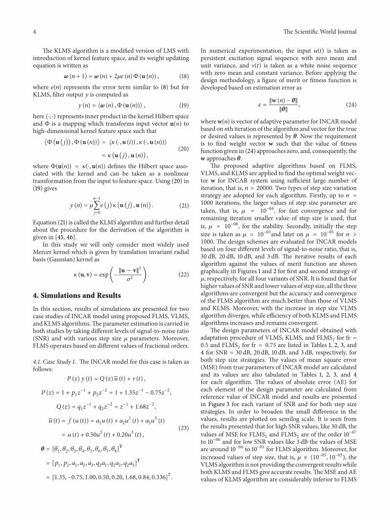
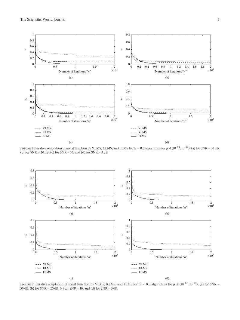
The proposed adaptive algorithms based on FLMS,VLMS, and KLMS are applied to find the optimal weight vec-tor w for INCAR system using sufficient large number ofiteration, that is, 𝑛 = 20000. Two types of step size variationstrategy are adopted for each algorithm. Firstly, up to 𝑛 =1000 iterations, the larger values of step size parameter aretaken, that is, 𝜇 = 10−04, for fast convergence and forremaining iteration smaller value of step size is used, thatis, 𝜇 = 10−08, for the stability. Secondly, initially the stepsize is taken as 𝜇 = 10−03and later on 𝜇 = 10−05 for 𝑛 >1000. The design schemes are evaluated for INCAR modelsbased on four different levels of signal-to-noise ratio, that is,30 dB, 20 dB, 10 dB, and 3 dB. The iterative results of eachalgorithm against the values of merit function are showngraphically in Figures 1 and 2 for first and second strategy of𝜇, respectively, for all four variants of SNR. It is found that forhigher values of SNRand lower values of step size, all the threealgorithms are convergent but the accuracy and convergenceof the FLMS algorithm are much better than those of VLMSand KLMS. Moreover, with the increase in step size VLMSalgorithm diverges, while efficiency of both KLMS and FLMSalgorithms increases and remains convergent.

The design parameters of INCAR model obtained withadaptation procedure of VLMS, KLMS, and FLMS

1for fr =

0.5 and FLMS2for fr = 0.75 are listed in Tables 1, 2, 3, and

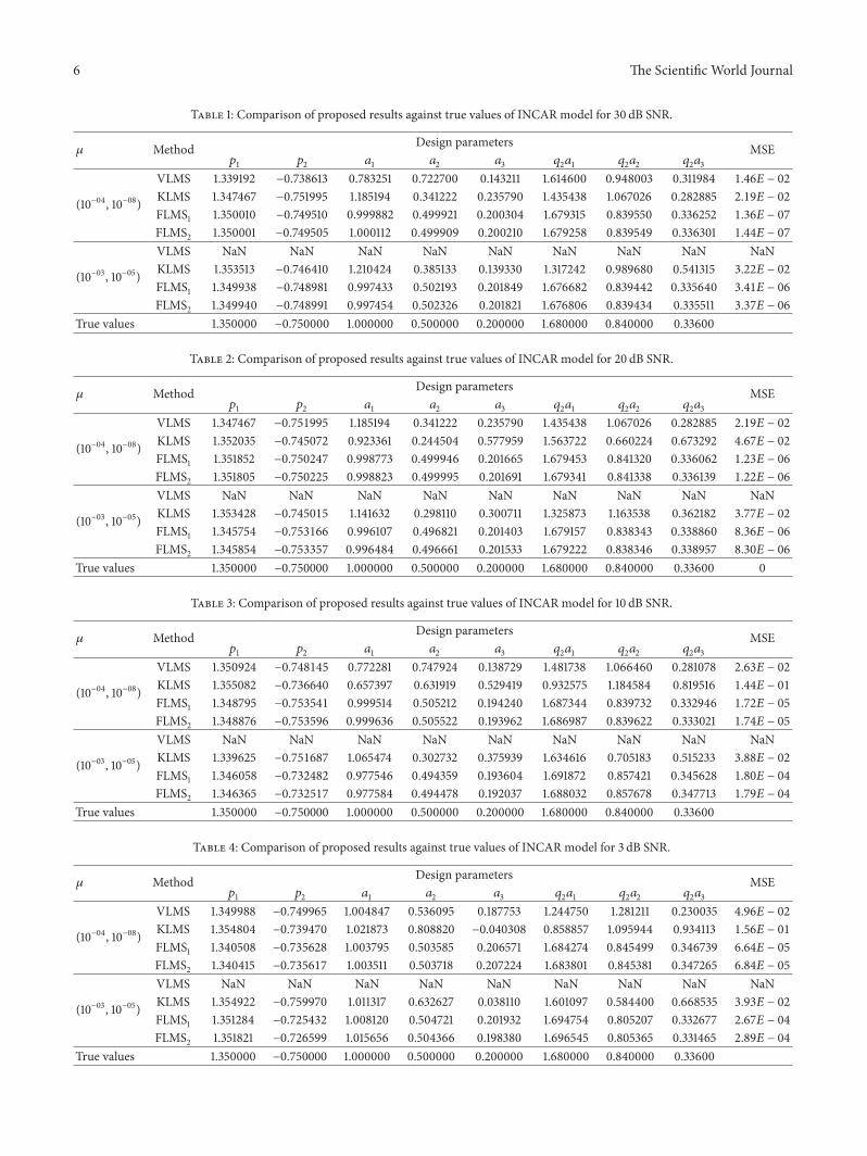
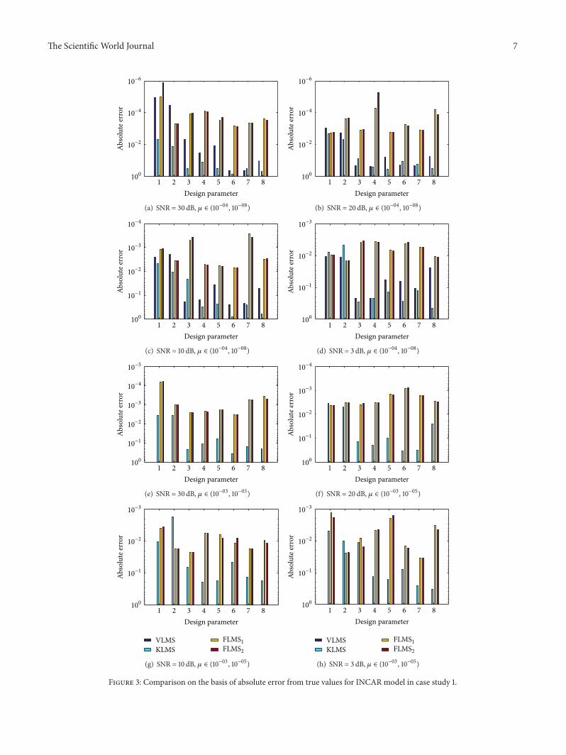
4 for SNR = 30 dB, 20 dB, 10 dB, and 3 dB, respectively, forboth step size strategies. The values of mean square error(MSE) from true parameters of INCAR model are calculatedand its values are also tabulated in Tables 1, 2, 3, and 4for each algorithm. The values of absolute error (AE) foreach element of the design parameter are calculated fromreference value of INCAR model and results are presentedin Figure 3 for each variant of SNR and for both step sizestrategies. In order to broaden the small difference in thevalues, results are plotted on semilog scale. It is seen fromthe results presented that for high SNR values, like 30 dB, thevalues of MSE for FLMS

1and FLMS

2are of the order 10−07

to 10−06 and for low SNR values like 3 dB the values of MSEare around 10−04 to 10−05 for FLMS algorithm. Moreover, forincreased values of step size, that is, 𝜇 ∈ (10−03, 10−05), theVLMSalgorithm is not providing the convergent resultswhileboth KLMS and FLMS give accurate results.TheMSE andAEvalues of KLMS algorithm are considerably inferior to FLMS


0 0.5 1 1.5 2×10

4

0

0.2

0.4

0.6

0.8

1

𝜀

Number of iterations “n”

(a)

21.81.61.41.210.80.60.40.20×10

4

0

0.2

0.4

0.6

0.8

𝜀


(b)

VLMSKLMSFLMS

21.81.61.41.210.80.60.40.20×10

4

0

0.2

0.4

0.6

0.8

1

𝜀


(c)

VLMSKLMSFLMS

×104

0

0.2

0.4

0.6

0.8

𝜀

0 0.5 1 1.5 2Number of iterations “n”

(d)

Figure 1: Iterative adaptation of merit function by VLMS, KLMS, and FLMS for fr = 0.5 algorithms for 𝜇 ∈ (10−04, 10−08); (a) for SNR = 30 dB,(b) for SNR = 20 dB, (c) for SNR = 10, and (d) for SNR = 3 dB.

0 0.5 1 1.5 2×10

4

0

0.2

0.4

0.6

0.8

𝜀


(a)

0 0.5 1 1.5 2×10

4

0

0.2

0.4

0.6

0.8

𝜀

1


(b)

0 0.5 1 1.5 2×10

4

0

0.2

0.4

0.6

0.8

𝜀

VLMSKLMSFLMS


(c)

0 0.5 1 1.5 2×10

4

0

0.2

0.4

0.6

0.8

𝜀

VLMSKLMSFLMS

1


(d)

Figure 2: Iterative adaptation of merit function by VLMS, KLMS, and FLMS for fr = 0.5 algorithms for 𝜇 ∈ (10−03, 10−05); (a) for SNR =30 dB, (b) for SNR = 20 dB, (c) for SNR = 10, and (d) for SNR = 3 dB.


Table 1: Comparison of proposed results against true values of INCAR model for 30 dB SNR.

𝜇 Method Design parameters MSE𝑝1

𝑝2

𝑎1

𝑎2

𝑎3

𝑞2𝑎1

𝑞2𝑎2

𝑞2𝑎3

(10−04, 10−08)

VLMS 1.339192 −0.738613 0.783251 0.722700 0.143211 1.614600 0.948003 0.311984 1.46𝐸 − 02

KLMS 1.347467 −0.751995 1.185194 0.341222 0.235790 1.435438 1.067026 0.282885 2.19𝐸 − 02

FLMS1 1.350010 −0.749510 0.999882 0.499921 0.200304 1.679315 0.839550 0.336252 1.36𝐸 − 07

FLMS2 1.350001 −0.749505 1.000112 0.499909 0.200210 1.679258 0.839549 0.336301 1.44𝐸 − 07

(10−03, 10−05)

VLMS NaN NaN NaN NaN NaN NaN NaN NaN NaNKLMS 1.353513 −0.746410 1.210424 0.385133 0.139330 1.317242 0.989680 0.541315 3.22𝐸 − 02

FLMS1 1.349938 −0.748981 0.997433 0.502193 0.201849 1.676682 0.839442 0.335640 3.41𝐸 − 06

FLMS2 1.349940 −0.748991 0.997454 0.502326 0.201821 1.676806 0.839434 0.335511 3.37𝐸 − 06

True values 1.350000 −0.750000 1.000000 0.500000 0.200000 1.680000 0.840000 0.33600



𝑝2

𝑎1

𝑎2

𝑎3

𝑞2𝑎1

𝑞2𝑎2

𝑞2𝑎3

(10−04, 10−08)

VLMS 1.347467 −0.751995 1.185194 0.341222 0.235790 1.435438 1.067026 0.282885 2.19𝐸 − 02

KLMS 1.352035 −0.745072 0.923361 0.244504 0.577959 1.563722 0.660224 0.673292 4.67𝐸 − 02

FLMS1 1.351852 −0.750247 0.998773 0.499946 0.201665 1.679453 0.841320 0.336062 1.23𝐸 − 06

FLMS2 1.351805 −0.750225 0.998823 0.499995 0.201691 1.679341 0.841338 0.336139 1.22𝐸 − 06

(10−03, 10−05)


FLMS1 1.345754 −0.753166 0.996107 0.496821 0.201403 1.679157 0.838343 0.338860 8.36𝐸 − 06

FLMS2 1.345854 −0.753357 0.996484 0.496661 0.201533 1.679222 0.838346 0.338957 8.30𝐸 − 06

True values 1.350000 −0.750000 1.000000 0.500000 0.200000 1.680000 0.840000 0.33600 0



𝑝2

𝑎1

𝑎2

𝑎3

𝑞2𝑎1

𝑞2𝑎2

𝑞2𝑎3

(10−04, 10−08)

VLMS 1.350924 −0.748145 0.772281 0.747924 0.138729 1.481738 1.066460 0.281078 2.63𝐸 − 02

KLMS 1.355082 −0.736640 0.657397 0.631919 0.529419 0.932575 1.184584 0.819516 1.44𝐸 − 01

FLMS1 1.348795 −0.753541 0.999514 0.505212 0.194240 1.687344 0.839732 0.332946 1.72𝐸 − 05

FLMS2 1.348876 −0.753596 0.999636 0.505522 0.193962 1.686987 0.839622 0.333021 1.74𝐸 − 05

(10−03, 10−05)


FLMS1 1.346058 −0.732482 0.977546 0.494359 0.193604 1.691872 0.857421 0.345628 1.80𝐸 − 04

FLMS2 1.346365 −0.732517 0.977584 0.494478 0.192037 1.688032 0.857678 0.347713 1.79𝐸 − 04

True values 1.350000 −0.750000 1.000000 0.500000 0.200000 1.680000 0.840000 0.33600



𝑝2

𝑎1

𝑎2

𝑎3

𝑞2𝑎1

𝑞2𝑎2

𝑞2𝑎3

(10−04, 10−08)

VLMS 1.349988 −0.749965 1.004847 0.536095 0.187753 1.244750 1.281211 0.230035 4.96𝐸 − 02

KLMS 1.354804 −0.739470 1.021873 0.808820 −0.040308 0.858857 1.095944 0.934113 1.56𝐸 − 01

FLMS1 1.340508 −0.735628 1.003795 0.503585 0.206571 1.684274 0.845499 0.346739 6.64𝐸 − 05

FLMS2 1.340415 −0.735617 1.003511 0.503718 0.207224 1.683801 0.845381 0.347265 6.84𝐸 − 05

(10−03, 10−05)


FLMS1 1.351284 −0.725432 1.008120 0.504721 0.201932 1.694754 0.805207 0.332677 2.67𝐸 − 04

FLMS2 1.351821 −0.726599 1.015656 0.504366 0.198380 1.696545 0.805365 0.331465 2.89𝐸 − 04

True values 1.350000 −0.750000 1.000000 0.500000 0.200000 1.680000 0.840000 0.33600


1 2 3 4 5 6 7 8Design parameter

10−6

10−4

10−2

100

Abso

lute

erro

r

(a) SNR = 30 dB, 𝜇 ∈ (10−04, 10−08)


10−6

10−4

10−2

100

Abso

lute

erro

r

(b) SNR = 20 dB, 𝜇 ∈ (10−04, 10−08)

1 2 3 4 5 6 7 8

10−4

10−3

10−2

10−1

100

Design parameter

Abso

lute

erro

r

(c) SNR = 10 dB, 𝜇 ∈ (10−04, 10−08)

1 2 3 4 5 6 7 8

10−3

10−2

10−1

100

Design parameter

Abso

lute

erro

r

(d) SNR = 3 dB, 𝜇 ∈ (10−04, 10−08)

1 2 3 4 5 6 7 8

10−5

10−4

10−3

10−2

10−1

100

Design parameter

Abso

lute

erro

r

(e) SNR = 30 dB, 𝜇 ∈ (10−03, 10−05)

1 2 3 4 5 6 7 8

10−4

10−3

10−2

10−1

100

Design parameter

Abso

lute

erro

r

(f) SNR = 20 dB, 𝜇 ∈ (10−03, 10−05)

1 2 3 4 5 6 7 8

10−3

10−2

10−1

100

Design parameter

Abso

lute

erro

r

VLMSKLMS

FLMS1

FLMS2

(g) SNR = 10 dB, 𝜇 ∈ (10−03, 10−05)

1 2 3 4 5 6 7 8

10−3

10−2

10−1

100

Design parameter

Abso

lute

erro

r

VLMSKLMS

FLMS1

FLMS2

(h) SNR = 3 dB, 𝜇 ∈ (10−03, 10−05)

Figure 3: Comparison on the basis of absolute error from true values for INCAR model in case study 1.


0 0.5 1 1.5 2×10

4

0

0.5

1

1.5

𝜀


(a)

0 0.2 0.4 0.6 0.8 1 1.2 1.4 1.6 1.8 2×10

4

0

0.2

0.4

0.6

0.8

𝜀


(b)

0 0.2 0.4 0.6 0.8 1 1.2 1.4 1.6 1.8 2×10

4

0

0.5

1

1.5

𝜀

VLMSKLMSFLMS


(c)

0 0.2 0.4 0.6 0.8 1 1.2 1.4 1.6 1.8 2×10

4

0

0.2

0.4

0.6

0.8

1

𝜀

VLMSKLMSFLMS


(d)

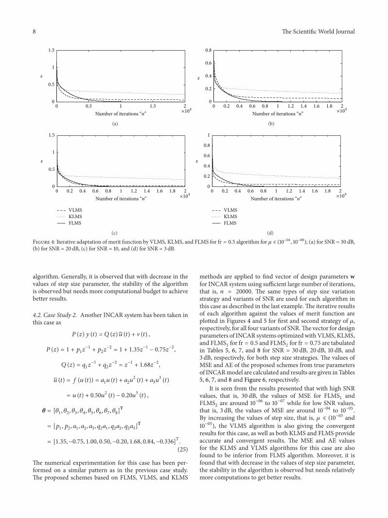
Figure 4: Iterative adaptation of merit function by VLMS, KLMS, and FLMS for fr = 0.5 algorithm for 𝜇 ∈ (10−04, 10−08); (a) for SNR = 30 dB,(b) for SNR = 20 dB, (c) for SNR = 10, and (d) for SNR = 3 dB.

algorithm. Generally, it is observed that with decrease in thevalues of step size parameter, the stability of the algorithmis observed but needs more computational budget to achievebetter results.

4.2. Case Study 2. Another INCAR system has been taken inthis case as

𝑃 (𝑧) 𝑦 (𝑡) = 𝑄 (𝑧) 𝑢 (𝑡) + V (𝑡) ,

𝑃 (𝑧) = 1 + 𝑝1𝑧−1+ 𝑝2𝑧−2= 1 + 1.35𝑧

−1− 0.75𝑧

−2,

𝑄 (𝑧) = 𝑞1𝑧−1+ 𝑞2𝑧−2= 𝑧−1+ 1.68𝑧

−2,

𝑢 (𝑡) = 𝑓 (𝑢 (𝑡)) = 𝑎1𝑢 (𝑡) + 𝑎

2𝑢2(𝑡) + 𝑎

3𝑢3(𝑡)

= 𝑢 (𝑡) + 0.50𝑢2(𝑡) − 0.20𝑢

3(𝑡) ,

𝜃 = [𝜃1, 𝜃2, 𝜃3, 𝜃4, 𝜃5, 𝜃6, 𝜃7, 𝜃8]T

= [𝑝1, 𝑝2, 𝑎1, 𝑎2, 𝑎3, 𝑞2𝑎1, 𝑞2𝑎2, 𝑞2𝑎3]T

= [1.35, −0.75, 1.00, 0.50, −0.20, 1.68, 0.84, −0.336]𝑇.

(25)

The numerical experimentation for this case has been per-formed on a similar pattern as in the previous case study.The proposed schemes based on FLMS, VLMS, and KLMS

methods are applied to find vector of design parameters wfor INCAR system using sufficient large number of iterations,that is, 𝑛 = 20000. The same types of step size variationstrategy and variants of SNR are used for each algorithm inthis case as described in the last example.The iterative resultsof each algorithm against the values of merit function areplotted in Figures 4 and 5 for first and second strategy of 𝜇,respectively, for all four variants of SNR.The vector for designparameters of INCAR systems optimizedwith VLMS, KLMS,and FLMS

1for fr = 0.5 and FLMS

2for fr = 0.75 are tabulated

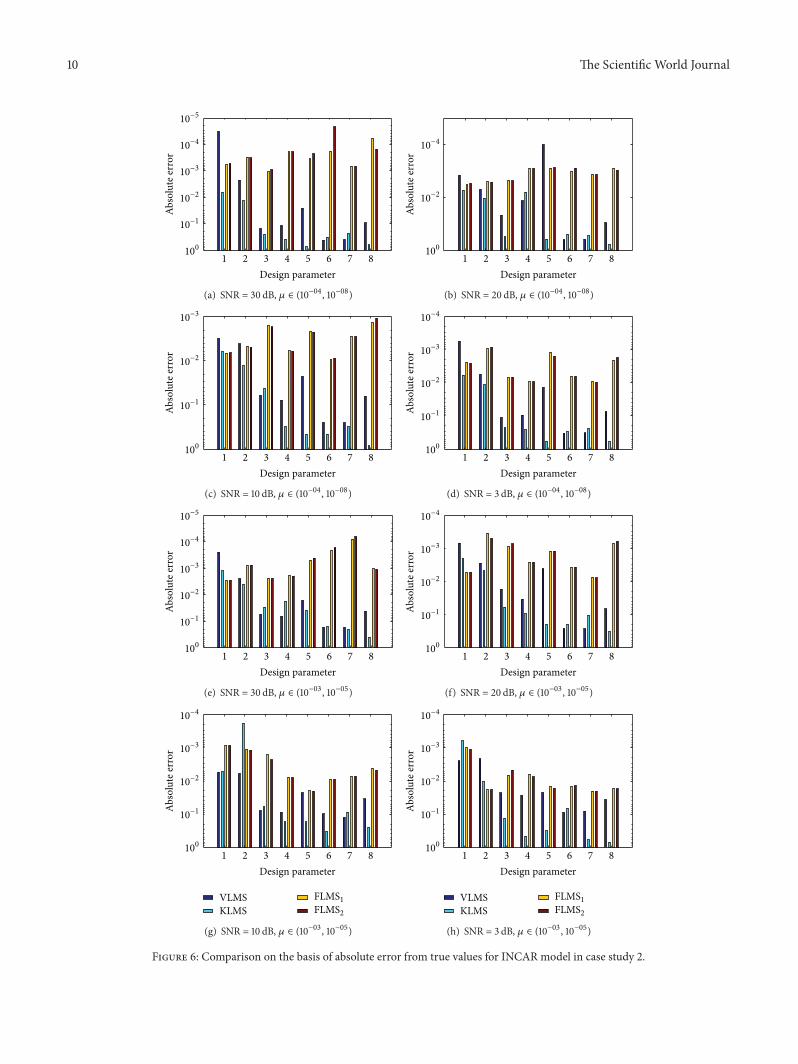
in Tables 5, 6, 7, and 8 for SNR = 30 dB, 20 dB, 10 dB, and3 dB, respectively, for both step size strategies. The values ofMSE and AE of the proposed schemes from true parametersof INCARmodel are calculated and results are given in Tables5, 6, 7, and 8 and Figure 6, respectively.

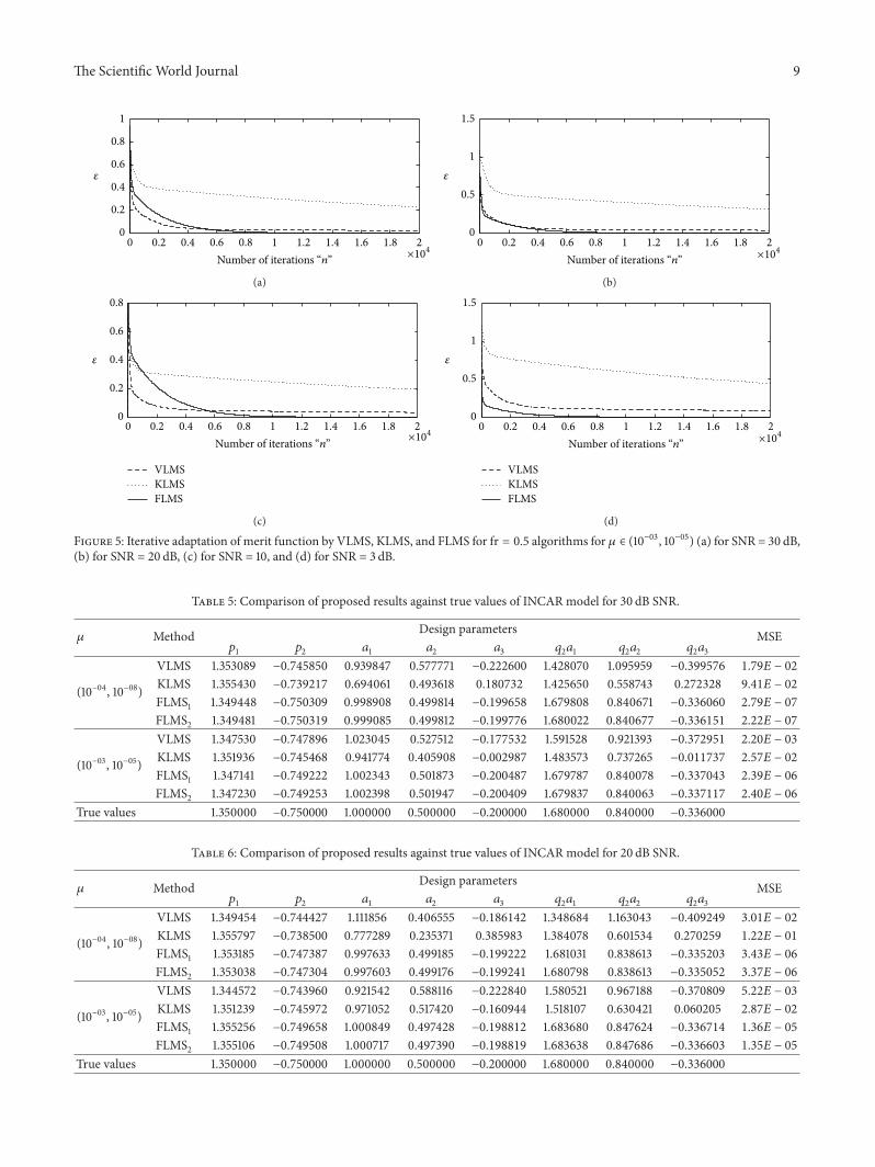
It is seen from the results presented that with high SNRvalues, that is, 30 dB, the values of MSE for FLMS

1and

FLMS2are around 10−06 to 10−07 while for low SNR values,

that is, 3 dB, the values of MSE are around 10−04 to 10−05.By increasing the values of step size, that is, 𝜇 ∈ (10−03 and10−05), the VLMS algorithm is also giving the convergentresults for this case, as well as both KLMS and FLMS provideaccurate and convergent results. The MSE and AE valuesfor the KLMS and VLMS algorithms for this case are alsofound to be inferior from FLMS algorithm. Moreover, it isfound that with decrease in the values of step size parameter,the stability in the algorithm is observed but needs relativelymore computations to get better results.


0 0.2 0.4 0.6 0.8 1 1.2 1.4 1.6 1.8 2×10

4

0

0.2

0.4

0.6

0.8

1

𝜀


(a)

0 0.2 0.4 0.6 0.8 1 1.2 1.4 1.6 1.8 2×10

4

1.5

1

0.5

0

𝜀


(b)

0 0.2 0.4 0.6 0.8 1 1.2 1.4 1.6 1.8 2×10

4

0

0.2

0.4

0.6

0.8

𝜀

VLMSKLMSFLMS


(c)

VLMSKLMSFLMS

0 0.2 0.4 0.6 0.8 1 1.2 1.4 1.6 1.8 2×10

4

1.5

1

0.5

0

𝜀


(d)

Figure 5: Iterative adaptation of merit function by VLMS, KLMS, and FLMS for fr = 0.5 algorithms for 𝜇 ∈ (10−03, 10−05) (a) for SNR = 30 dB,(b) for SNR = 20 dB, (c) for SNR = 10, and (d) for SNR = 3 dB.



𝑝2

𝑎1

𝑎2

𝑎3

𝑞2𝑎1

𝑞2𝑎2

𝑞2𝑎3

(10−04, 10−08)

VLMS 1.353089 −0.745850 0.939847 0.577771 −0.222600 1.428070 1.095959 −0.399576 1.79𝐸 − 02

KLMS 1.355430 −0.739217 0.694061 0.493618 0.180732 1.425650 0.558743 0.272328 9.41𝐸 − 02

FLMS1 1.349448 −0.750309 0.998908 0.499814 −0.199658 1.679808 0.840671 −0.336060 2.79𝐸 − 07

FLMS2 1.349481 −0.750319 0.999085 0.499812 −0.199776 1.680022 0.840677 −0.336151 2.22𝐸 − 07

(10−03, 10−05)

VLMS 1.347530 −0.747896 1.023045 0.527512 −0.177532 1.591528 0.921393 −0.372951 2.20𝐸 − 03

KLMS 1.351936 −0.745468 0.941774 0.405908 −0.002987 1.483573 0.737265 −0.011737 2.57𝐸 − 02

FLMS1 1.347141 −0.749222 1.002343 0.501873 −0.200487 1.679787 0.840078 −0.337043 2.39𝐸 − 06

FLMS2 1.347230 −0.749253 1.002398 0.501947 −0.200409 1.679837 0.840063 −0.337117 2.40𝐸 − 06

True values 1.350000 −0.750000 1.000000 0.500000 −0.200000 1.680000 0.840000 −0.336000



𝑝2

𝑎1

𝑎2

𝑎3

𝑞2𝑎1

𝑞2𝑎2

𝑞2𝑎3

(10−04, 10−08)

VLMS 1.349454 −0.744427 1.111856 0.406555 −0.186142 1.348684 1.163043 −0.409249 3.01𝐸 − 02

KLMS 1.355797 −0.738500 0.777289 0.235371 0.385983 1.384078 0.601534 0.270259 1.22𝐸 − 01

FLMS1 1.353185 −0.747387 0.997633 0.499185 −0.199222 1.681031 0.838613 −0.335203 3.43𝐸 − 06

FLMS2 1.353038 −0.747304 0.997603 0.499176 −0.199241 1.680798 0.838613 −0.335052 3.37𝐸 − 06

(10−03, 10−05)

VLMS 1.344572 −0.743960 0.921542 0.588116 −0.222840 1.580521 0.967188 −0.370809 5.22𝐸 − 03

KLMS 1.351239 −0.745972 0.971052 0.517420 −0.160944 1.518107 0.630421 0.060205 2.87𝐸 − 02

FLMS1 1.355256 −0.749658 1.000849 0.497428 −0.198812 1.683680 0.847624 −0.336714 1.36𝐸 − 05

FLMS2 1.355106 −0.749508 1.000717 0.497390 −0.198819 1.683638 0.847686 −0.336603 1.35𝐸 − 05

True values 1.350000 −0.750000 1.000000 0.500000 −0.200000 1.680000 0.840000 −0.336000



10−5

10−4

10−3

10−2

10−1

100

Abso

lute

erro

r

(a) SNR = 30 dB, 𝜇 ∈ (10−04, 10−08)


10−4

10−2

100

Abso

lute

erro

r

(b) SNR = 20 dB, 𝜇 ∈ (10−04, 10−08)


10−3

10−2

10−1

100

Abso

lute

erro

r

(c) SNR = 10 dB, 𝜇 ∈ (10−04, 10−08)


10−4

10−3

10−2

10−1

100

Abso

lute

erro

r

(d) SNR = 3 dB, 𝜇 ∈ (10−04, 10−08)


10−5

10−4

10−3

10−2

10−1

100

Abso

lute

erro

r

(e) SNR = 30 dB, 𝜇 ∈ (10−03, 10−05)


10−4

10−3

10−2

10−1

100

Abso

lute

erro

r

(f) SNR = 20 dB, 𝜇 ∈ (10−03, 10−05)

VLMSKLMS

FLMS1

FLMS2


10−4

10−3

10−2

10−1

100

Abso

lute

erro

r

(g) SNR = 10 dB, 𝜇 ∈ (10−03, 10−05)

VLMSKLMS

FLMS1

FLMS2


10−4

10−3

10−2

10−1

100

Abso

lute

erro

r

(h) SNR = 3 dB, 𝜇 ∈ (10−03, 10−05)

Figure 6: Comparison on the basis of absolute error from true values for INCAR model in case study 2.




𝑝2

𝑎1

𝑎2

𝑎3

𝑞2𝑎1

𝑞2𝑎2

𝑞2𝑎3

(10−04, 10−08)

VLMS 1.351468 −0.744938 1.047010 0.486303 −0.200102 1.285267 1.225023 −0.427779 3.94𝐸 − 02

KLMS 1.356262 −0.736962 0.956832 0.185102 0.259909 1.220949 0.529005 0.495796 1.64𝐸 − 01

FLMS1 1.356850 −0.745266 1.001581 0.494077 −0.202190 1.670903 0.837135 −0.334630 2.56𝐸 − 05

FLMS2 1.356608 −0.745109 1.001695 0.493895 −0.202230 1.671239 0.837177 −0.334908 2.48𝐸 − 05

(10−03, 10−05)

VLMS 1.349757 −0.747542 0.945167 0.564599 −0.216172 1.511909 1.011739 −0.377157 8.36𝐸 − 03

KLMS 1.355306 −0.750178 1.058421 0.333366 −0.033855 1.341960 0.926972 −0.080043 3.08𝐸 − 02

FLMS1 1.350819 −0.748919 0.998394 0.491951 −0.179965 1.688782 0.847405 −0.340293 7.76𝐸 − 05

FLMS2 1.350853 −0.748833 0.997694 0.492029 −0.179449 1.688987 0.847312 −0.340771 8.13𝐸 − 05

True values 1.350000 −0.750000 1.000000 0.500000 −0.200000 1.680000 0.840000 −0.336000



𝑝2

𝑎1

𝑎2

𝑎3

𝑞2𝑎1

𝑞2𝑎2

𝑞2𝑎3

(10−04, 10−08)

VLMS 1.350033 −0.747776 1.151411 0.382217 −0.174445 1.266046 1.237098 −0.428614 4.69𝐸 − 02

KLMS 1.356493 −0.736365 0.748964 0.105174 0.542420 1.362022 0.609956 0.290923 1.65𝐸 − 01

FLMS1 1.352386 −0.750941 0.992991 0.491026 −0.198780 1.686456 0.849316 −0.338108 3.38𝐸 − 05

FLMS2 1.352534 −0.750836 0.993316 0.490747 −0.198439 1.686445 0.849539 −0.337726 3.44𝐸 − 05

(10−03, 10−05)

VLMS 1.349324 −0.747288 0.983402 0.533690 −0.203984 1.423701 1.105389 −0.402156 1.77𝐸 − 02

KLMS 1.350614 −0.760252 1.136970 0.030726 0.119125 1.612852 0.232501 0.372932 1.52𝐸 − 01

FLMS1 1.351001 −0.731407 0.993154 0.493843 −0.214263 1.694738 0.819746 −0.318643 1.95𝐸 − 04

FLMS2 1.351107 −0.731604 0.995350 0.492513 −0.216675 1.693931 0.819381 −0.318775 2.01𝐸 − 04

True values 1.350000 −0.750000 1.000000 0.500000 −0.200000 1.680000 0.840000 −0.336000

5. Conclusion

On the basis of the simulation and results presented in the lastsection, the following conclusions are drawn.

(i) The adaptive algorithms based on fractional signalprocessing approach are used effectively for param-eter estimation of input nonlinear control autoregres-sive (INCAR) models for both case studies.

(ii) The variation of step size strategies shows that forsmaller and relatively larger value of step size parame-ter both order of fractional least mean square (FLMS)algorithms provide accurate and convergent resultsthan those of VLMS and KLMS algorithms.

(iii) The variants of signal-to-noise ratio (SNR) in INCARmodels show that the performance of all the algo-rithm decreases as SNR decreases from higher levelto lower level, but FLMS algorithm still achieved thevalues for mean square error around 10−04 to 10−05 foreven SNR = 3 dB.

(iv) Comparative studies between FLMS, VLMS, andKLMS algorithms for each variants of both case stud-ies validate the correctness of the adaptive algorithmsbased on FLMS algorithm.

In future, one may look for heuristic computing techniquesbased on genetic algorithms, swarm intelligence, differentialevolution, genetic programming, and memetic computing

approaches, and so forth, for parameter estimation of INCARmodels.

References

[1] M. R. Zakerzadeh, M. Firouzi, H. Sayyaadi, and S. B. Shouraki,“Hysteresis nonlinearity identification using new Preisachmodel-based artificial neural network approach,” Journal ofApplied Mathematics, vol. 2011, Article ID 458768, 22 pages,2011.

[2] X. X. Li, H. Z. Guo, S. M. Wan, and F. Yang, “Inverse sourceidentification by the modified regularization method on pois-son equation,” Journal of AppliedMathematics, vol. 2012, ArticleID 971952, 13 pages, 2012.

[3] Y. Shi and H. Fang, “Kalman filter-based identification forsystems with randomly missing measurements in a networkenvironment,” International Journal of Control, vol. 83, no. 3, pp.538–551, 2010.

[4] Y. Liu, J. Sheng, and R. Ding, “Convergence of stochastic gradi-ent estimation algorithm for multivariable ARX-like systems,”Computers andMathematics with Applications, vol. 59, no. 8, pp.2615–2627, 2010.

[5] F. Ding, G. Liu, and X. P. Liu, “Parameter estimation with scarcemeasurements,” Automatica, vol. 47, no. 8, pp. 1646–1655, 2011.

[6] J. Ding, F. Ding, X. P. Liu, andG. Liu, “Hierarchical least squaresidentification for linear SISO systems with dual-rate sampled-data,” IEEE Transactions on Automatic Control, vol. 56, no. 11,pp. 2677–2683, 2011.


[7] Y. Liu, Y. Xiao, and X. Zhao, “Multi-innovation stochastic gra-dient algorithm for multiple-input single-output systems usingthe auxiliary model,” Applied Mathematics and Computation,vol. 215, no. 4, pp. 1477–1483, 2009.

[8] J. Ding and F. Ding, “The residual based extended least squaresidentification method for dual-rate systems,” Computers andMathematics with Applications, vol. 56, no. 6, pp. 1479–1487,2008.

[9] L. Han and F. Ding, “Identification for multirate multi-inputsystems using themulti-innovation identification theory,”Com-puters and Mathematics with Applications, vol. 57, no. 9, pp.1438–1449, 2009.

[10] F. Ding, Y. Shi, and T. Chen, “Gradient-based identificationmethods for hammerstein nonlinear ARMAXmodels,”Nonlin-ear Dynamics, vol. 45, no. 1-2, pp. 31–43, 2006.

[11] F. Ding, T. Chen, and Z. Iwai, “Adaptive digital control ofHammerstein nonlinear systems with limited output sampling,”SIAM Journal on Control and Optimization, vol. 45, no. 6, pp.2257–2276, 2007.

[12] F. Ding and T. Chen, “Identification of Hammerstein nonlinearARMAX systems,” Automatica, vol. 41, no. 9, pp. 1479–1489,2005.

[13] I. W. Hunter and M. J. Korenberg, “The identification ofnonlinear biological systems: wiener andHammerstein cascademodels,” Biological Cybernetics, vol. 55, no. 2-3, pp. 135–144,1986.

[14] Y. Y. Cao and Z. Lin, “Robust stability analysis and fuzzy-scheduling control for nonlinear systems subject to actuator sat-uration,” IEEE Transactions on Fuzzy Systems, vol. 11, no. 1, pp.57–67, 2003.

[15] K. P. Fruzzetti, A. Palazoglu, and K. A. McDonald, “Nonlinearmodel predictive control using Hammerstein models,” Journalof Process Control, vol. 7, no. 1, pp. 31–41, 1997.

[16] S. Dupont and J. Luettin, “Audio-visual speech modeling forcontinuous speech recognition,” IEEE Transactions onMultime-dia, vol. 2, no. 3, pp. 141–151, 2000.

[17] M. Karimi-Ghartemani and M. R. Iravani, “A nonlinear adap-tive filter for online signal analysis in power systems: applica-tions,” IEEE Transactions on Power Delivery, vol. 17, no. 2, pp.617–622, 2002.

[18] F. Ding and T. Chen, “Identification of Hammerstein nonlinearARMAX systems,” Automatica, vol. 41, no. 9, pp. 1479–1489,2005.

[19] F. Ding, Y. Shi, and T. Chen, “Auxiliary model-based least-squares identification methods for Hammerstein output-errorsystems,” Systems and Control Letters, vol. 56, no. 5, pp. 373–380,2007.

[20] B. B. Mandelbrot and J. W. Van Ness, “Fractional Brownianmotions, fractional noises and applications,” SIAM Review, vol.10, no. 4, pp. 422–437, 1968.

[21] L. Gaul, P. Klein, and S. Kemple, “Damping description involv-ing fractional operators,” Mechanical Systems and Signal Pro-cessing, vol. 5, no. 2, pp. 81–88, 1991.

[22] J. Sabatier, M. Aoun, A. Oustaloup, G. Gregoire, F. Ragot, and P.Roy, “Fractional system identification for lead acid battery stateof charge estimation,” Signal Processing, vol. 86, no. 10, pp. 2645–2657, 2006.

[23] M. D. Ortigueira, J. A. Tenreiro Machado, and J. S. da Costa,“Which differintegration? [fractional calculus],” IEE Proceed-ings: Vision Image and Signal Processing, vol. 152, no. 6, pp. 846–850, 2005.

[24] D. Valerio, M. D. Ortigueira, and J. Sa da Costa, “Identifying atransfer function from a frequency response,” ASME Journal ofComputational and Nonlinear Dynamics, vol. 3, no. 2, Article ID021207, 7 pages, 2008.

[25] M. D. Ortigueira, “Introduction to fractional linear systems.Part 1: continuous-time case,” IEE Proceedings: Vision, Imageand Signal Processing, vol. 147, no. 1, pp. 62–70, 2000.

[26] M. D. Ortigueira, “Introduction to fractional linear systems.Part 2: discrete-time case,” IEE Proceedings: Vision, Image andSignal Processing, vol. 147, no. 1, pp. 71–78, 2000.

[27] M. D. Ortigueira and J. A. TenreiroMachado, “Fractional signalprocessing and applications,” Signal Processing, vol. 83, no. 11, pp.2285–2286, 2003.

[28] M. D. Ortigueira and J. A. T. Machado, “Fractional calculusapplications in signals and systems,” Signal Processing, vol. 86,no. 10, pp. 2503–2504, 2006.

[29] E. Cuesta,M. Kirane, and S. A.Malik, “Image structure preserv-ing denoising using generalized fractional time integrals,” SignalProcessing, vol. 92, no. 2, pp. 553–563, 2012.

[30] C. C. Tseng and S. L. Lee, “Design of adjustable fractional orderdifferentiator using expansion of ideal frequency response,”Signal Processing, vol. 92, no. 2, pp. 498–508, 2012.

[31] W. Fan, F. Ding, and Y. Shi, “Parameter estimation for Hammer-stein nonlinear controlled auto-regression models,” in Proceed-ings of the IEEE International Conference on Automation andLogistics (ICAL ’07), pp. 1007–1012, August 2007.

[32] X.Weili,W. Fan, and R.Ding, “Least-squares parameter estima-tion algorithm for a class of input nonlinear systems,” Journalof Applied Mathematics, vol. 2012, Article ID 684074, 14 pages,2012.

[33] R. M. A. Zahoor and I. M. Qureshi, “A modified least meansquare algorithm using fractional derivative and its applicationto system identification,”European Journal of Scientific Research,vol. 35, no. 1, pp. 14–21, 2009.

[34] M. Geravanchizadeh and S. G. Osgouei, “Dual-channel speechenhancement using normalized fractional least-mean-squaresalgorithm,” in Proceedings of the 19th Iranian Conference onElectrical Engineering (ICEE ’11), May 2011.

[35] S. G. Osgouei and M. Geravanchizadeh, “Speech enhancementusing convex combination of fractional least-mean-squaresalgorithm,” in Proceedings of the 5th International Symposiumon Telecommunications (IST ’10), pp. 869–872, December 2010.

[36] D. S. Kumar and N. K. Rout, “FLMS algorithm for acousticecho cancellation and its comparison with LMS,” in Proceedingsof the IEEE 1st International Conference on Recent Advances inInformation Technology (RAIT ’12), pp. 852–856, March 2012.

[37] A. Pervez and M. Yasin, “Performance analysis of bessel beam-former and LMS algorithm for smart antenna array in mobilecommunication system,” Emerging Trends and Applications inInformation Communication Technologies, vol. 281, pp. 52–61,2012.

[38] M. Yasin and P. Akhtar, “Performance analysis of bessel beam-former with LMS algorithm for smart antenna array,” in Pro-ceeding of the International Conference on Open Source Systemsand Technologies (ICOSST ’12), pp. 1–5, December 2012.

[39] S. Haykin, Adaptive Filter Theory (ISE), 2003.[40] R. M. A. Zahoor, Application of fractional calculus to engineer-

ing: a new computational approach [Ph.D. thesis], InternationalIslamic University, Islamabad, Pakistan, 2011.

[41] B. Georgeta, Nonlinear Systems Identification Using the VolterraModel, University of Timisoara, 2005.


[42] A. Guerin, G. Faucon, and R. Le Bouquin-Jeannes, “Nonlinearacoustic echo cancellation based on volterra filters,” IEEETransactions on Speech and Audio Processing, vol. 11, no. 6, pp.672–683, 2003.

[43] F. Kuch and W. Kellermann, “Nonlinear line echo cancellationusing a simplified second order Volterra filter,” in Proceedings ofthe IEEE International Conference onAcoustic, Speech and SignalProcessing, vol. 2, pp. 1117–1120, May 2002.

[44] B. Georgeta and C. Botoca, “Nonlinearities identification usingthe LMS Volterra filter,” in Proceedings of the WSEAS Interna-tional Conference on Dynamical Systems and Control, pp. 148–153, Communications Department, Faculty of Electronics andTelecommunications, Venice, Italy, November 2005.

[45] P. P. Pokharel, L. Weifeng, and J. C. Principe, “Kernel LMS,” inProceedings of the IEEE International Conference on Acoustics,Speech and Signal Processing (ICASSP ’07, vol. 3, pp. 1421–1424,April 2007.

[46] W. Liu, P. P. Pokharel, and J. C. Principe, “Thekernel least-mean-square algorithm,” IEEE Transactions on Signal Processing, vol.56, no. 2, pp. 543–554, 2008.

[47] A. Gunduz, J. P. Kwon, J. C. Sanchez, and J. C. Principe, “Decod-ing hand trajectories from ECoG recordings via kernel least-mean-square algorithm,” in Proceedings of the 4th InternationalIEEE/EMBS Conference on Neural Engineering (NER ’09), pp.267–270, May 2009.

[48] B. Pantelis, S. Theodoridis, and M. Mavroforakis, “The aug-mented complex kernel LMS,” IEEE Transactions on SignalProcessing, vol. 60, no. 9, pp. 4962–4967, 2012.

[49] H. Bao and I. M. S. Panahi, “Active noise control based onkernel least-mean-square algorithm,” in Proceedings of the 43rdAsilomar Conference on Signals, Systems and Computers, pp.642–644, November 2009.

International Journal of

AerospaceEngineeringHindawi Publishing Corporationhttp://www.hindawi.com Volume 2014

RoboticsJournal of

Hindawi Publishing Corporationhttp://www.hindawi.com Volume 2014


Active and Passive Electronic Components

Control Scienceand Engineering

Journal of



RotatingMachinery


Hindawi Publishing Corporation http://www.hindawi.com

Journal ofEngineeringVolume 2014

Submit your manuscripts athttp://www.hindawi.com

VLSI Design



Shock and Vibration


Civil EngineeringAdvances in

Acoustics and VibrationAdvances in



Electrical and Computer Engineering

Journal of

Advances inOptoElectronics

Hindawi Publishing Corporation http://www.hindawi.com

Volume 2014

The Scientific World JournalHindawi Publishing Corporation http://www.hindawi.com Volume 2014

SensorsJournal of


Modelling & Simulation in EngineeringHindawi Publishing Corporation http://www.hindawi.com Volume 2014


Chemical EngineeringInternational Journal of Antennas and

Propagation




Navigation and Observation



DistributedSensor Networks


Documents

Research Article Identification of Input Nonlinear Control Autoregressive Systems ...downloads.hindawi.com/journals/tswj/2013/467276.pdf · 2019-07-31 · 2. Input Nonlinear Control