Embed Size (px)
Citation preview
903
Sigma J Eng & Nat Sci 37 (3), 2019, 903-916
Research Article
NUMERICAL MODELLING OF SUDDEN CONTRACTION IN PIPE FLOW
Engin GÜCÜYEN*1, Recep Tuğrul ERDEM
2, Ümit GÖKKUŞ
3
1Manisa Celal Bayar University, Department of Civil Engineering, MANISA; ORCID: 0000-0001-9971-8546 2Manisa Celal Bayar University, Department of Civil Engineering, MANISA; ORCID: 0000-0002-8895-7602 3Manisa Celal Bayar University, Department of Civil Engineering, MANISA; ORCID: 0000-0002-2422-6392
Received: 31.01.2019 Revised: 03.05.2019 Accepted: 14.06.2019
ABSTRACT
In the present work, full-scale numerical simulations of incompressible fluid flow through different locations
of sudden contractions are studied according to Computational Fluid Dynamics (CFD) technique. Finite Elements Method is used to numerically solve governing equations via the commercial program ABAQUS
including CFD code. Four different locations of contraction zone are utilized to determine the effect of
location changes on sudden contraction head loss coefficients (KC). Twelve area ratios () are performed for all zones. Three different Reynolds numbers, remain in laminar flow boundaries, are adopted to determine
effects of Reynolds number, as well as location effects. The graphs are constituted by results from computing
48 models for each Reynolds number and the study is concluded with 144 models in the end. In this manner, contraction ratio varying coefficients are obtained for four configurations. According to results, the pressure
drop values of the same model for varying contraction locations are different. Maximum values of pressure
drops are obtained for the second geometry (G2). Combination of maximum pressure drops and minimum velocity values leads to maximum contraction coefficients for G2. While the area coefficients increase,
decreasing values of contraction coefficients of different contraction locations (G) converge in connection
with the changing values of velocities and pressure drops. It is necessary to entrain to this remark, for
increasing area coefficients. It is stated that KC- curves vary due to location change. It is recommended to
consider the location varying coefficients while modelling different located contracting flows especially for
side contracting flows. Keywords: Sudden contraction coefficients, contraction location effects, computational fluid dynamics, finite
elements.
1. INTRODUCTION
Sudden contraction applications are widely used in different fields of engineering including
civil, nuclear, mechanical, chemical, pharmaceutical, food, bio and biomedical. Contraction or
expansion problems are only ceased to be the subject of civil and mechanical engineering by
developing multi-disciplinary engineering approaches such as bio engineering. As an example, a
sudden contraction of a blood vessel has started to be studied by likened pipe flow [1, 2, 3].
Cross section area of pipe flow may change according to sediment erosion, the location, fluid
pipe transports and intended purpose. If the change in pipe cross-section is gradual, no flow
* Corresponding Author: e-mail: [email protected], tel: (236) 201 23 21
Sigma Journal of Engineering and Natural Sciences
Sigma Mühendislik ve Fen Bilimleri Dergisi
904
separation occurs and the c hange of static pressure may effectively convert to the kinetic energy.
However, if there is a sudden change in the flow area, it may cause a significant loss due to
additional turbulence arising in the connection [4-11]. Each type of loss can be quantified by
using a loss coefficient (KC). Velocity of flow and geometry of device directly effect the amount
of losses. A significant amount of pressure drop occurs due to sudden contraction in pipe by
increasing the velocity and the losing energy.
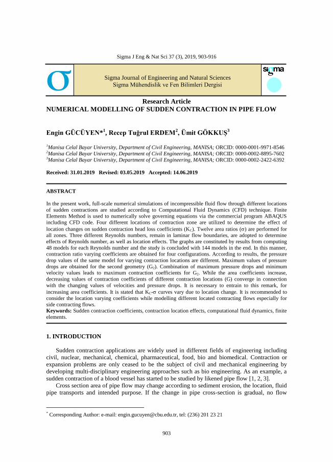
The changes are encountered as contraction or expansion. In this study, contraction problem is
deeply investigated. The simple geometrical configuration of contracting flow is formed by two
pipes having different diameters [13]. As well as this simple form, more complex coaxially form
can be seen in connected pipes of different diameters. Coaxial contraction will be separately
located at the side, at the top [14], and the bottom [6]. One co axial and three with coaxial
scenarios that are studied in this paper are seen in Figure 1. The diameter ratio of inlet to outlet
pipe is taken as the main geometric parameter which is referred to as the area ratio, () [15, 16].
Figure 1. Geometrical models in analyses
Its geometrical simplicity and hydrodynamic complexity make sudden contraction as an ideal
problem for testing various numerical methods. As a result, a wealth of literature exists on such a
flow covering a wide range of fluids and governing parameters. In addition to other methods such
as Finite Volume Method [11, 17, 18], Finite Elements Method can be implemented in numerical
studies as utilized in this study [19, 20, 21].
This study is aimed at determining contraction location on sudden contraction coefficients
which is called (KC). For this purpose, four geometrical scenarios are set out including one co
axial and three with coaxial sudden contracting geometries. In the modelling phase, twelve
different diameter ratios of outlet to inlet of the pipe are utilized for all geometries. As a result,
forty-eight geometries are modelled in total. The models under consideration have undergone
three inlet velocities to determine Reynolds number effects as well as location effects. ABAQUS
[22] Finite Elements Analysis program is used to perform analyses. It is seen that KC values that
are obtained after analysis are compatible with the previous studies in the literature [23, 24].
2. NUMERICAL STUDY
A numerical investigation into the effect of contraction location changes on the sudden
contraction coefficients of single-phase flow in full-scale models has been conducted in this
paper. In the first stage of the study, geometrical models are generated to evaluate the numerical
analyses. According to the results which are obtained from analyses, the contraction coefficients
are calculated and effects of location on sudden contraction coefficients are determined.
2.1. Geometrical Models
In this study, four geometrical configurations each of them including twelve contraction ratios
are investigated. First configuration is commonly used as coaxial contracting flow. In this
configuration, both normal axis (z) of inlet and outlet flow are located in the same axis. The other
configurations are formed as with coaxial contracting flows. The normal axis of inlet and outlet
flows is not randomly located. With coaxial contracting configurations are composed of side, top
and bottom ones are contracting models. The sudden contraction geometries consist of two pipes.
While the first one is inlet, the other one is outlet. Inlet flow diameter (D) is maintained constant
E. Gücüyen, R.T. Erdem, Ü. Gökkuş / Sigma J Eng & Nat Sci 37 (3), 903-916, 2019
905
throughout this study and it is equal to 1 m. Outlet flow diameters (d) vary between 0.30 and 0.85
with 0.05 increments as given in Table 1.
Table 1. Diameters of inlet and outlet pipes
D (m) 1.00 1.00 1.00 1.00 1.00 1.00 1.00 1.00 1.00 1.00 1.00 1.00
d (m) 0.30 0.35 0.40 0.45 0.50 0.55 0.60 0.65 0.70 0.75 0.80 0.85
0.090 0.123 0.160 0.203 0.250 0.303 0.360 0.423 0.490 0.563 0.640 0.723
The values which are taken from well-known contraction coefficient graphic [24] have been
utilized to calculate area ratios (). This ratio is the geometry range that is defined by the
contraction area ratio from outlet (Ad) to inlet (AD) corresponding to the diameter d and D
respectively.
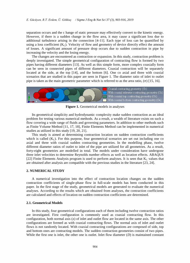
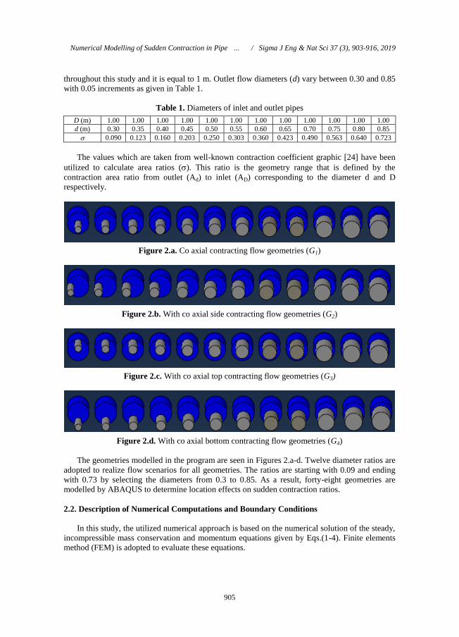
Figure 2.a. Co axial contracting flow geometries (G1)
Figure 2.b. With co axial side contracting flow geometries (G2)
Figure 2.c. With co axial top contracting flow geometries (G3)
Figure 2.d. With co axial bottom contracting flow geometries (G4)
The geometries modelled in the program are seen in Figures 2.a-d. Twelve diameter ratios are
adopted to realize flow scenarios for all geometries. The ratios are starting with 0.09 and ending
with 0.73 by selecting the diameters from 0.3 to 0.85. As a result, forty-eight geometries are
modelled by ABAQUS to determine location effects on sudden contraction ratios.
2.2. Description of Numerical Computations and Boundary Conditions
In this study, the utilized numerical approach is based on the numerical solution of the steady,
incompressible mass conservation and momentum equations given by Eqs.(1-4). Finite elements
method (FEM) is adopted to evaluate these equations.
Numerical Modelling of Sudden Contraction in Pipe … / Sigma J Eng & Nat Sci 37 (3), 903-916, 2019
906
( u) ( v) ( w) 0x y z
(1)
2 2 22
2 2 2
u P u u u( u ) ( uv) ( uw)
t x y z x x y z
(2)
2 2 22
2 2 2
v P v v v( uv) ( v ) ( vw)
t x y z y x y z
(3)
2 2 22
2 2 2
w P w w w( uw) ( vw) ( w )
t x y z z x y z
(4)
In Eqs.(1-4) u, v and w are the velocity components at the x, y and z coordinate directions
respectively. ρ, μ and P stand for the density, the dynamic viscosity and the pressure. In this
study, the fluid is incompressible and Newtonian. The regime is stationary. The used fluid is
water, at temperature of 20 C. The other properties are used as follows: ρ=988.2 kg/m3 and
μ=1004.10-6 m2/s. Average velocity values of 0.80 m/s, 1.20 m/s and 1.60 m/s have been used as
normal uniform velocity inlet boundary condition in this work. In this manner, effect of Reynolds
number on contraction coefficient can be seen. The velocity at the inlet is parallel to the inlet flow
axis without cross stream components [24]. Zero pressure value and no streamwise variation for
velocity components have been set at the outlet boundary. At the remaining domain surfaces are
set non-slip wall boundary conditions. The boundary conditions that are described above, can be
mathematically represented in Table 2. [19]. Eqs.(1-4) are solved abiding the boundary conditions
via [22].
Table 2. Boundary conditions
Surfaces Boundary Conditions
Inlet u0, v=w=0
Outlet P=0, u/x+v/x+w/x=0
Non-slip walls u=v=w=0
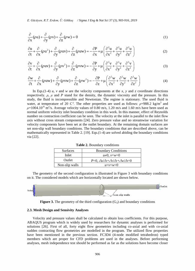
The geometry of the second configuration is illustrated in Figure 3 with boundary conditions
on it. The considered models which are horizontally located are shown below.
Figure 3. The geometry of the third configuration (G3) and boundary conditions
2.3. Mesh Design and Sensivity Analyses
Velocity and pressure values shall be calculated to obtain loss coefficients. For this purpose,
ABAQUS program which is widely used by researchers for dynamic analyses is performed for
solutions [26]. First of all, forty eight flow geometries including co-axial and with co-axial
sudden contracting flow geometries are modelled in the program. The utilized flow properties
have been mentioned in the previous section. FC3D4 (4-node modified tetrahedron) typed
members which are proper for CFD problems are used in the analyses. Before performing
analyses, mesh independence test should be performed as far as the solutions have become closer
E. Gücüyen, R.T. Erdem, Ü. Gökkuş / Sigma J Eng & Nat Sci 37 (3), 903-916, 2019
907
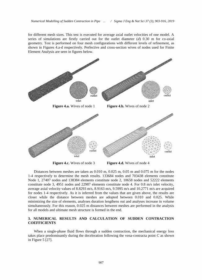
for different mesh sizes. This test is executed for average axial outlet velocities of one model. A
series of simulations are firstly carried out for the outlet diameter (d) 0.30 m for co-axial
geometry. Test is performed on four mesh configurations with different levels of refinement, as
shown in Figures 4.a-d respectively. Perfective and cross-section wives of nodes used for Finite
Element Analysis are seen in figures below.
Figure 4.a. Wives of node 1 Figure 4.b. Wives of node 2
Figure 4.c. Wives of node 3 Figure 4.d. Wives of node 4
Distances between meshes are taken as 0.010 m, 0.025 m, 0.05 m and 0.075 m for the nodes
1-4 respectively to determine the mesh results. 133684 nodes and 703438 elements constitute
Node 1, 27407 nodes and 138384 elements constitute node 2, 10658 nodes and 52222 elements
constitute node 3, 4951 nodes and 22987 elements constitute node 4. For 0.8 m/s inlet velocity,
average axial velocity values of 8.8293 m/s, 8.9163 m/s, 9.5995 m/s and 10.2771 m/s are acquired
for nodes 1-4 respectively. As it is inferred from the values that are given above, the results are
closer while the distance between meshes are adopted between 0.010 and 0.025. While
minimizing the size of elements, analyses duration lengthens out and analyses increase in volume
simultaneously. For this reason, 0.025 m distances between meshes are performed in the analysis
for all models and ultimate mesh structure is formed in the end.
3. NUMERICAL RESULTS AND CALCULATION OF SUDDEN CONTRACTION
COEFFICIENTS
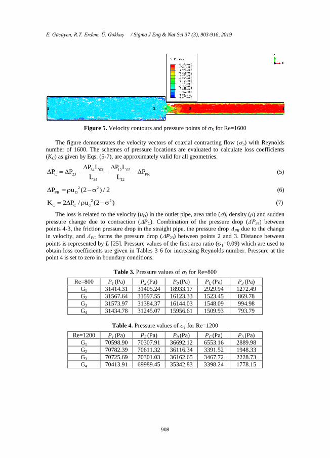
When a single-phase fluid flows through a sudden contraction, the mechanical energy loss
takes place predominantly during the deceleration following the vena-contracta point C as shown
in Figure 5 [27].
Numerical Modelling of Sudden Contraction in Pipe … / Sigma J Eng & Nat Sci 37 (3), 903-916, 2019
908
Figure 5. Velocity contours and pressure points of 5 for Re=1600
The figure demonstrates the velocity vectors of coaxial contracting flow (5) with Reynolds
number of 1600. The schemes of pressure locations are evaluated to calculate loss coefficients
(KC) as given by Eqs. (5-7), are approximately valid for all geometries.
34 03 12 02
C 23 PR
34 12
P L P LP P P
L L
(5)
2 2
PR DP u (2 ) / 2 (6)
2 2
C C dK 2 P / u (2 ) (7)
The loss is related to the velocity (uD) in the outlet pipe, area ratio (), density (ρ) and sudden
pressure change due to contraction (PC). Combination of the pressure drop (ΔP34) between
points 4-3, the friction pressure drop in the straight pipe, the pressure drop ΔPR due to the change
in velocity, and ΔPC forms the pressure drop (P23) between points 2 and 3. Distance between
points is represented by L [25]. Pressure values of the first area ratio (1=0.09) which are used to
obtain loss coefficients are given in Tables 3-6 for increasing Reynolds number. Pressure at the
point 4 is set to zero in boundary conditions.
Table 3. Pressure values of 1 for Re=800
Re=800 P1 (Pa) P2 (Pa) P0 (Pa) PC (Pa) P3 (Pa)
G1 31414.31 31405.24 18933.17 2929.94 1272.49
G2 31567.64 31597.55 16123.33 1523.45 869.78
G3 31573.97 31384.37 16144.03 1548.09 994.98
G4 31434.78 31245.07 15956.61 1509.93 793.79
Table 4. Pressure values of 1 for Re=1200
Re=1200 P1 (Pa) P2 (Pa) P0 (Pa) PC (Pa) P3 (Pa)
G1 70598.90 70307.91 36692.12 6553.16 2889.98
G2 70782.39 70611.32 36116.34 3391.52 1948.33
G3 70725.69 70301.03 36162.65 3467.72 2228.73
G4 70413.91 69989.45 35342.83 3398.24 1778.15
E. Gücüyen, R.T. Erdem, Ü. Gökkuş / Sigma J Eng & Nat Sci 37 (3), 903-916, 2019
909
Table 5. Pressure values of 1 for Re=1600
Re=1600 P1 (Pa) P2 (Pa) P0 (Pa) PC (Pa) P3 (Pa)
G1 126009.52 125490.2 65490.52 11796.55 5158.23
G2 125658.32 124904.2 64250.12 6001.09 3459.78
G3 124074.11 123329.2 63440.17 6083.42 3909.86
G4 119048.82 120330.4 60430.42 5939.64 3006.24
Although finite elements analyses of all models are performed by Finite Elements Program,
results of all models are not given. Only three of them are presented including 1, 6 and 12 as
example solutions. Pressure values of 6 are given between Tables 6-8.
Table 6. Pressure values of 6 for Re=800
Re=800 P1 (Pa) P2 (Pa) P0 (Pa) PC (Pa) P3 (Pa)
G1 6501.23 6207.8 3233.6 384.78 181.68
G2 6571.92 6580.21 2831.65 438.20 185.32
G3 6645.98 6610.07 3305.48 509.85 229.21
G4 6751.81 6702.02 3206.68 499.45 212.19
Table 7. Pressure values of 6 for Re=1200
Re=1200 P1 (Pa) P2 (Pa) P0 (Pa) PC (Pa) P3 (Pa)
G1 15129.24 15089.02 7953.89 613.01 270.35
G2 15318.45 15226.23 7199.89 636.18 358.17
G3 15354.32 15281.41 7225.91 638.48 410.36
G4 15311.5 15047.52 7115.25 672.10 383.84
Table 8. Pressure values of 6 for Re=1600
Re=1600 P1 (Pa) P2 (Pa) P0 (Pa) PC (Pa) P3 (Pa)
G1 27239.1 26577.3 14118.1 1105.4 425.07
G2 26743.62 26735.90 11876.10 994.75 432.0282
G3 27802.83 27791.30 13742.60 1215.31 694.0647
G4 27855.47 27688.20 13651.80 1112.23 650.5676
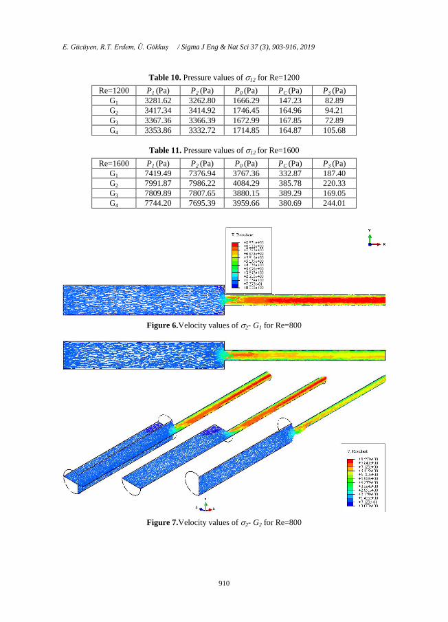
The pressure values at certain nodes for 12 are given between Table 9 and Table 11 for
increasing Re number.
Table 9. Pressure values of 12 for Re=800
Re=800 P1 (Pa) P2 (Pa) P0 (Pa) PC (Pa) P3 (Pa)
G1 1451.45 1451.03 721.12 72.35 31.42
G2 1461.26 1452.44 741.75 65.54 36.92
G3 1451.89 1451.28 741.56 70.04 40.04
G4 1452.49 1443.76 742.67 71.21 45.77
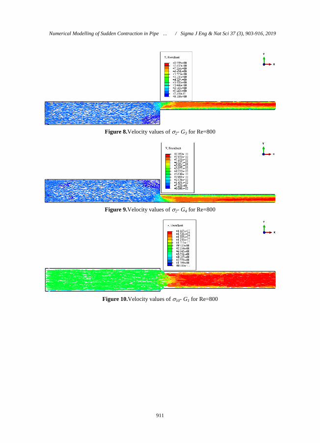
As it can be easily understood from Eq. (7), not only pressure drops but also velocity values
are effective on sudden contraction coefficients. Therefore, velocity values should also be given.
In terms of referring to different samples, results of 2 and 10 which have not taken part in
previous figures are given between Figures 6-13. The flow geometries are vertically cut in vertical
axis (y), as it is in the middle of contraction region. Unlike other geometries, there is a need to
give all views of G2 because of having unsymmetrical contraction location.
Numerical Modelling of Sudden Contraction in Pipe … / Sigma J Eng & Nat Sci 37 (3), 903-916, 2019
910
Table 10. Pressure values of 12 for Re=1200
Re=1200 P1 (Pa) P2 (Pa) P0 (Pa) PC (Pa) P3 (Pa)
G1 3281.62 3262.80 1666.29 147.23 82.89
G2 3417.34 3414.92 1746.45 164.96 94.21
G3 3367.36 3366.39 1672.99 167.85 72.89
G4 3353.86 3332.72 1714.85 164.87 105.68
Table 11. Pressure values of 12 for Re=1600
Re=1600 P1 (Pa) P2 (Pa) P0 (Pa) PC (Pa) P3 (Pa)
G1 7419.49 7376.94 3767.36 332.87 187.40
G2 7991.87 7986.22 4084.29 385.78 220.33
G3 7809.89 7807.65 3880.15 389.29 169.05
G4 7744.20 7695.39 3959.66 380.69 244.01
Figure 6.Velocity values of 2- G1 for Re=800
Figure 7.Velocity values of 2- G2 for Re=800
E. Gücüyen, R.T. Erdem, Ü. Gökkuş / Sigma J Eng & Nat Sci 37 (3), 903-916, 2019
911
Figure 8.Velocity values of 2- G3 for Re=800
Figure 9.Velocity values of 2- G4 for Re=800
Figure 10.Velocity values of 10- G1 for Re=800
Numerical Modelling of Sudden Contraction in Pipe … / Sigma J Eng & Nat Sci 37 (3), 903-916, 2019
912
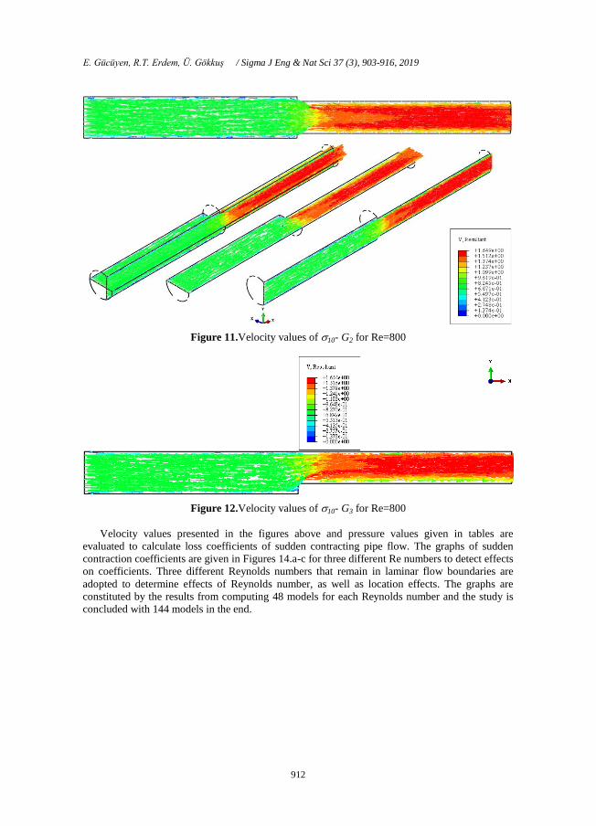
Figure 11.Velocity values of 10- G2 for Re=800
Figure 12.Velocity values of 10- G3 for Re=800
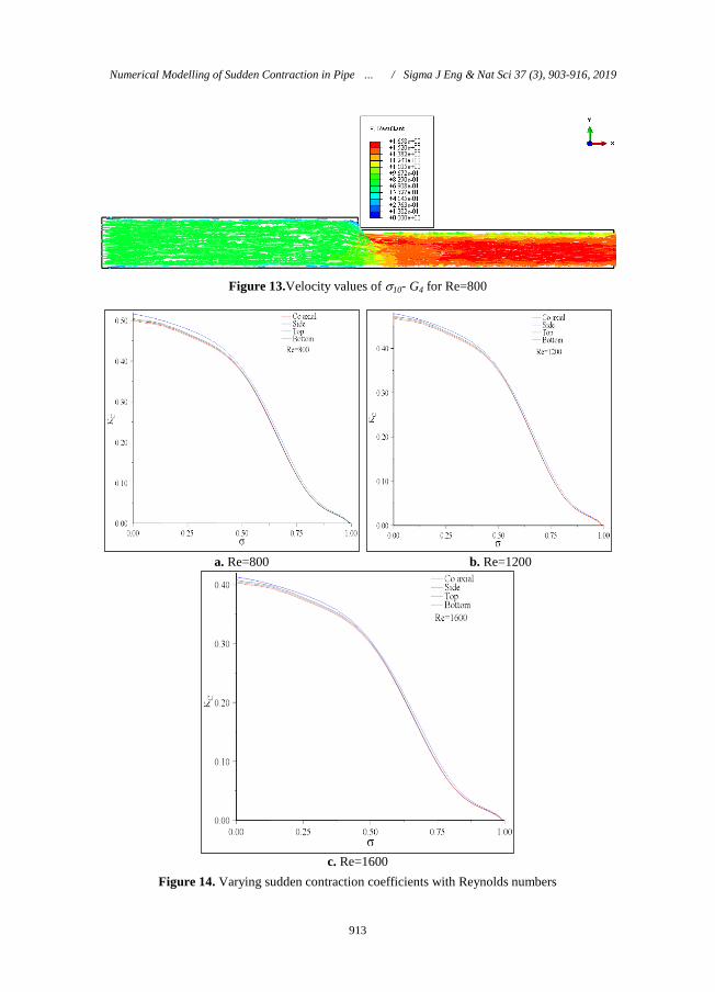
Velocity values presented in the figures above and pressure values given in tables are
evaluated to calculate loss coefficients of sudden contracting pipe flow. The graphs of sudden
contraction coefficients are given in Figures 14.a-c for three different Re numbers to detect effects
on coefficients. Three different Reynolds numbers that remain in laminar flow boundaries are
adopted to determine effects of Reynolds number, as well as location effects. The graphs are
constituted by the results from computing 48 models for each Reynolds number and the study is
concluded with 144 models in the end.
E. Gücüyen, R.T. Erdem, Ü. Gökkuş / Sigma J Eng & Nat Sci 37 (3), 903-916, 2019
913
Figure 13.Velocity values of 10- G4 for Re=800
a. Re=800 b. Re=1200
c. Re=1600
Figure 14. Varying sudden contraction coefficients with Reynolds numbers
Numerical Modelling of Sudden Contraction in Pipe … / Sigma J Eng & Nat Sci 37 (3), 903-916, 2019
914
It is known from the previous studies in the literature that values of contraction head loss
coefficients vary between 0.00 and 0.50. It is presented in Figure 14 that obtained results after
numerical analyses remain between the expected values.
4. CONCLUSIONS
In this paper, it is aimed to detect effects of changes of contraction locations on sudden
contraction coefficients. In order to determine these efxfects, large scaled specimens including 48
models are numerically studied and analysed via ABAQUS. While performing the regular
analyses, the sensitivity analyses are carried out simultaneously. Node distances are determined as
0.025 m according the sensitivity analyses.
The contraction coefficients are directly effected by three parameters; area ratios, velocity and
pressure drop respectively. While an inlet and outlet narrowing flow geometries are connected,
increase in velocity and energy losses occur and this situation induces drop of pressure. In
previous studies, the effects of varying area ratios and velocities on contraction coefficients have
already been studied. But it is known that, the outlet pipe will be connected to different locations
of inlet pipe such as at the side, top and bottom. In this study, effect of location changes on
contraction coefficients are examined by means of Figures 6-13 and Tables 3-11. These results
are obtained from only a portion of 144 models. The graph covering all of the model results is
given in Figure 14. In this figure, both Reynolds number and area ratio varying loss coefficients
are presented.
Although having the same boundary conditions and mesh structure same model () produce
different velocity values for different contraction locations (G). The outlet velocity values adopted
to calculate coefficients are given between Figures 6-9 for 2 and between Figures 10-13 for 10 in
which Re is 800. While the values of 2 are 8.871 m/s, 8.553 m/s, 8.659 m/s and 8.703 m/s, the
values of 10 are 1.667 m/s, 1.649 m/s, 1.654 m/s and 1.658 m/s for G1, G2, G3 and G4
respectively. Minimum value is obtained for side contracting with coaxial flow and the maximum
one is obtained for coaxial contracting flow for both models. The difference brings out the
contraction location between minimum and maximum values is 3.58% for 2 and 1.02% for 10.
The results reveal that the differences between outlet velocity values of the models decrease
unlike the increase in . Same situation is observed for all models mentioned in this study. The
difference approximately reverberates on contraction coefficients regarding the differences of
drop of pressure. The analyses have been performed for increasing Re number and it is stated that
the loss coefficient is decreasing for increasing Re numbers, as it has been mentioned in previous
studies.
Based on the results given in Tables 3-11, one can easily indicate that drop of pressure values
of the same model for varying contraction locations are different. According to mentioned tables,
maximum values of pressure drops are obtained for G2. Combination of maximum drop of
pressure, minimum velocity values leads to obtain maximum contraction coefficients for G2.
While the area coefficients increase, decreasing values of contraction coefficients of different
contraction locations (G) converge are seen in Figures 14.a-c, due to converging values of
velocities and drop of pressure. It is necessary to entrain to this remark, for increasing area
coefficients.
It is determined that values of contraction head loss coefficients are approximately same with
the general used values. In addition to this, new values are obtained in case of contraction in
different locations. New values that are obtained from different locations are close to the values
obtained from co axial contraction. These values have been presented by figures and tables in the
study. This situation is the main reason of using co axial contraction coefficient in case of
different location contraction in practice.
Although not being mentioned in past studies, with coaxial contracting models are widely
used in industrial applications which are the starting point of this study. The results predicate this
E. Gücüyen, R.T. Erdem, Ü. Gökkuş / Sigma J Eng & Nat Sci 37 (3), 903-916, 2019
915
starting point. It is recommended to take into consideration the location varying coefficients while
modelling different located contracting flows especially for side contracting flows. The approach
of this study will be implementing to sudden expansion problems for further studies.
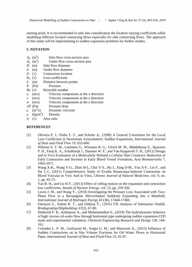
5. NOTATION
AD (m2) Inlet flow cross-section area
Ad (m2) Outlet flow cross-section area
D (m) Inlet flow diameter
d (m) Outlet flow diameter
G (1) Contraction location
KC (1) Loss coefficients
L (m) Distance between points
P (Pa) Pressure
Re (1) Reynolds number
u (m/s) Velocity components at the x direction
v (m/s) Velocity components at the y direction
w (m/s) Velocity components at the z direction
ΔP (Pa) Pressure drop
μ (m2/s) Dynamic viscosity
ρ (kg/m3) Density
(1) Area ratio
REFERENCES
[1] Oliveira P. J., Pinho F. T., and Schulte A., (1998) A General Correlation for the Local
Loss Coefficient in Newtonian Axisymmetric Sudden Expansions, International Journal
of Heat and Fluid Flow 19, 655-660.
[2] Nillesen S. T. M., Lammers G., Wismans R. G., Ulrich M. M., Middelkoop E., Spauwen
P. H., Faraj K. A., Schalkwijk J., Daamen W. F., and Van Kuppevelt T. H., (2011) Design
and in Vivo Evaluation of a Molecularly Defined a Cellular Skin Construct: Reduction of
Early Contraction and Increase in Early Blood Vessel Formation, Acta Biomaterialia 7,
1063-1071.
[3] Wang X-K., Wang Y-G., Zhan H-L, Chai Y-S., Hu J., Xing D-M., You X-F., Lei F., and
Du L-J., (2011) Comprehensive Study of Evodia Rutaecarpa-Induced Contraction on
Blood Vascular in Vivo And in Vitro, Chinese Journal of Natural Medicines, vol. 9, no.
1, pp. 65-73.
[4] Yan B. H., and Gu H.Y., (2013) Effect of rolling motion on the expansion and contraction
loss coefficients, Annals of Nuclear Energy, vol. 53, pp, 259-266.
[5] Lewis J. M., and Wang Y., (2018) Investigating the Pressure Loss Associated with Two-
Phase Flow in a Rectangular Microchannel Suddenly Expanding into a Manifold,
International Journal of Hydrogen Energy 43 (36), 17444-17460.
[6] Gücüyen E., Erdem R. T., and Gökkuş Ü., (2016) FSI Analysis of Submarine Outfall,
Brodogradnja/Shipbuilding, 67(2), 67-80.
[7] Dehkordi P. B., Azdarpour A., and Mohammadian E., (2018) The hydrodynamic behavior
of high viscous oil-water flow through horizontal pipe undergoing sudden expansion-CFD
study and experimental validation, Chemical Engineering Research and Design 139, 144-
161.
[8] Colombo L. P. M., Guilizzoni M., Sotgia G. M., and Marzorati D., (2015) Influence of
Sudden Contractions on in Situ Volume Fractions for Oil–Water Flows in Horizontal
Pipes, International Journal of Heat and Fluid Flow 53, 91-97.
Numerical Modelling of Sudden Contraction in Pipe … / Sigma J Eng & Nat Sci 37 (3), 903-916, 2019
916
[9] Bae Y., and Kim, Y.I., (2014) Prediction of Local Loss Coefficient for Turbulent Flow in
Axisymmetric Sudden Expansions with a Chamfer: Effect of Reynolds Number, Annals of
Nuclear Energy 73, 33-38.
[10] Javadi A., and Nilsson H., (2015) LES and DES of Strongly Swirling Turbulent Flow
Through a Suddenly Expanding Circular Pipe, Computers & Fluids 107, 301-313
[11] Badr H. M., Habib M. A., Ben-Mansour R., and Said, S. A. M., (2005) Numerical
Investigation of Erosion Threshold Velocity in a Pipe with Sudden Contraction,
Computers & Fluids 34, 721–742.
[12] Ala A. A., Tan S., Eltayeb A., Abbati Z., (2019) Experimental Study on Sudden
Contraction and Split into the Inlets of Two Parallel Rectangular Jets, Experimental
Thermal and Fluid Science 104, 272, 283.
[13] Chalfi T. Y., and Ghiaasiaan S. M., (2008) Pressure Drop Caused by Flow Area Changes
in Capillaries under Low Flow Conditions, International Journal of Multiphase Flow 34,
2-12.
[14] Hammad K. J., and Vradis G. C., (1996) Creeping Flow of a Bingham Plastic Through
Axisymmetric Sudden Contractions with Viscous Dissipation, International Journal of
Heat Mass Transfer 39(8), 1555-1567.
[15] Yesilata B., Öztekin A., and Neti S., (1999) Instabilities in Viscoelastic Flow Through an
Axisymmetric Sudden Contraction, Journal of Non-Newtonian Fluid Mechanics 85, 35-
62.
[16] Yesilata B., Öztekin A., and Neti S., (2000) Non-isothermal viscoelastic flow through an
axisymmetric sudden contraction Journal of Non-Newtonian Fluid Mechanic 89, 133-164.
[17] Cherrared D., and Filali E. G., (2013) Hydrodynamics and Heat Transfer in Two and
Three-Dimensional Minichannels, Fluid Dynamics and Materials Processing, 9( 2), 127-
151.
[18] Holmesa L., Faverob J., and Osswald T., (2012) Numerical Simulation of Three-
Dimensional Viscoelastic Planar Contraction Flow Using the Software Open FOAM,
Computers and Chemical Engineering 37, 64-73.
[19] Lima R. C., Andrade C. R., and Zaparoli E. L., (2008) Numerical Study of Three
Recirculation Zones in the Unilateral Sudden Expansion Flow, International
Communications in Heat and Mass Transfer 35, 1053–1060.
[20] Kaushik V. V. R., Ghosh S., Das G., and Das P. K., (2012) CFD Simulation of Core
Annular Flow Through Sudden Contraction and Expansion, Journal of Petroleum Science
and Engineering 86–87, 153-164.
[21] Schrecka E., and Schafer M., (2000) Numerical Study of Bifurcation in Three-
Dimensional Sudden Channel Expansions, Computers & Fluids 29, 583-593.
[22] ABAQUS User's Manual (2010), Version 6.10.
[23] Cengel Y. A., Cimbala J. M., (2014). Fluid Mechanics Fundamentals and
Applications, Mc Graw Hill, New York, USA.
[24] Shaughnessy E.J., Katz I. M., and Schaffer J. P., (2005) Introduction to Fluid Mechanics,
Oxford University Press, New York, USA.
[25] Guo B., Langrish T. A. G., and Fletcher D. F., (1998) Simulation of Precession in
Axisymmetric Sudden Expansion Flows, Second International Conference on CFD in the
Minerals and Process Industries, Csıro, Melbourne, Australia.
[26] Gücüyen E., and Erdem R T., (2018) Beton Kazıklı Açık Deniz Yapısının Analizi, Selçuk
Üniversitesi Mühendislik, Bilim ve Teknoloji Dergisi 6(4), 767-778.
[27] Guo H., Wang L., Yu J., Ye F., Ma C., and Li Z. (2010) Local resistance of fluid flow
across sudden contraction in small channels, Frontiers of Energy and Power Engineering
in China, vol. 4, no. 2, pp. 149-154.
E. Gücüyen, R.T. Erdem, Ü. Gökkuş / Sigma J Eng & Nat Sci 37 (3), 903-916, 2019