Embed Size (px)
Citation preview
Hindawi Publishing CorporationISRN OpticsVolume 2013 Article ID 108704 8 pageshttpdxdoiorg1011552013108704
Research ArticlePerturbation Analysis with Approximate Integration forPropagation Mode in Two-Dimensional Two-Slab Waveguides
Naofumi Kitsunezaki
Department of Integrated Information Technology College of Science and Engineering Aoyama Gauin UniversitySagamihara-shi Kanagawa 252-5258 Japan
Correspondence should be addressed to Naofumi Kitsunezaki kitsunezakiitaoyamaacjp
Received 23 May 2013 Accepted 14 July 2013
Academic Editors Z Chen S Wade and D-n Wang
Copyright copy 2013 Naofumi Kitsunezaki This is an open access article distributed under the Creative Commons AttributionLicense which permits unrestricted use distribution and reproduction in any medium provided the original work is properlycited
On the basis of perturbation expansion from a gapless system we calculate the propagation constant and propagation mode wavefunction in two-dimensional two-slab waveguides with a core gap small enough that there is only one propagation mode We alsoperform calculations without the approximation for comparison Our result shows that first-order perturbation contains the first-order Taylor expansion of (core gap)(core width) and when the integration of the perturbation is suitably approximated the resultof the first-order perturbation is the same as that of the first-order Taylor expansion of (core gap)(core width)
1 Introduction
When monochromatic light enters into one of the cores ofa waveguide array in which each core has the same widthand the same gap the light propagates to adjacent coresin turn and its trajectory becomes V-shaped Such opticalbehavior has been theoretically and numerically analyzedTheoretical analysis includes matrix method [1] the coupledmode equation and the coupled power equation [2ndash9] Inthe coupling mode equations it is assumed that there is atleast one propagation mode for each core and that all of thepropagation modes are independent from each other
This assumption is invalid in the case that the number ofindependent propagation modes is less than the number ofcores Such a situation can occur when the core gap becomessmall enough that the index distribution is approximated by agapless core When such a situation occurs analysis based onthe coupled mode or the coupled power equation is invalidOur interest is finding a simple method to analyze an opticalbehavior in such a situation
An optical behavior for parallel slab waveguides withsmall core gap was theoretically analyzed using even and oddmode analysis which was called supermode analysis later[3ndash5] In this analysis the exact solution for the Maxwellrsquos
equations with the index distribution for two parallel slabwaveguides which becomes essentially one for Schrodingerequation for double finite wells in the field of quantummechanics is used to analyze the optical behavior Howeverthemethod using supermodes is not useful when the numberof cores increases because the solution must be individuallyexpressed in every core and clad
In the field of quantum mechanics perturbation theoryis widely used as an approximation [10 11] In the field ofelectromagnetics and optics it is also explained in [12] andapplied to explain bend losses for a fiber [13 14] Coupledmode equation is also based on the perturbation theory [4ndash7] The situation that we are interested in is suitable for usingthe perturbation theory
In this paper we calculate the supermode for a two-dimensional two-slab waveguide that has a small core gapso that the optical system has only one propagation modeusing first-order perturbation from gapless system We alsocalculate the same without approximation for comparison Inthis way we show that first-order perturbation with suitableapproximate integration and the first-order Taylor expansionof (core gap)(core width) give the same result Furthermorewe discuss higher-order relationships between perturbationwith suitable approximate integration and Taylor expansion
2 ISRN Optics
Clad (n2) Clad (n2)
x
z
w2 + dminusw2 minus d minusw2 w2
Core (n1) Core (n1)
y
(a)
n2
n1
xw2 + dminusw2 minus d minusw2 w2
n(x)
(b)
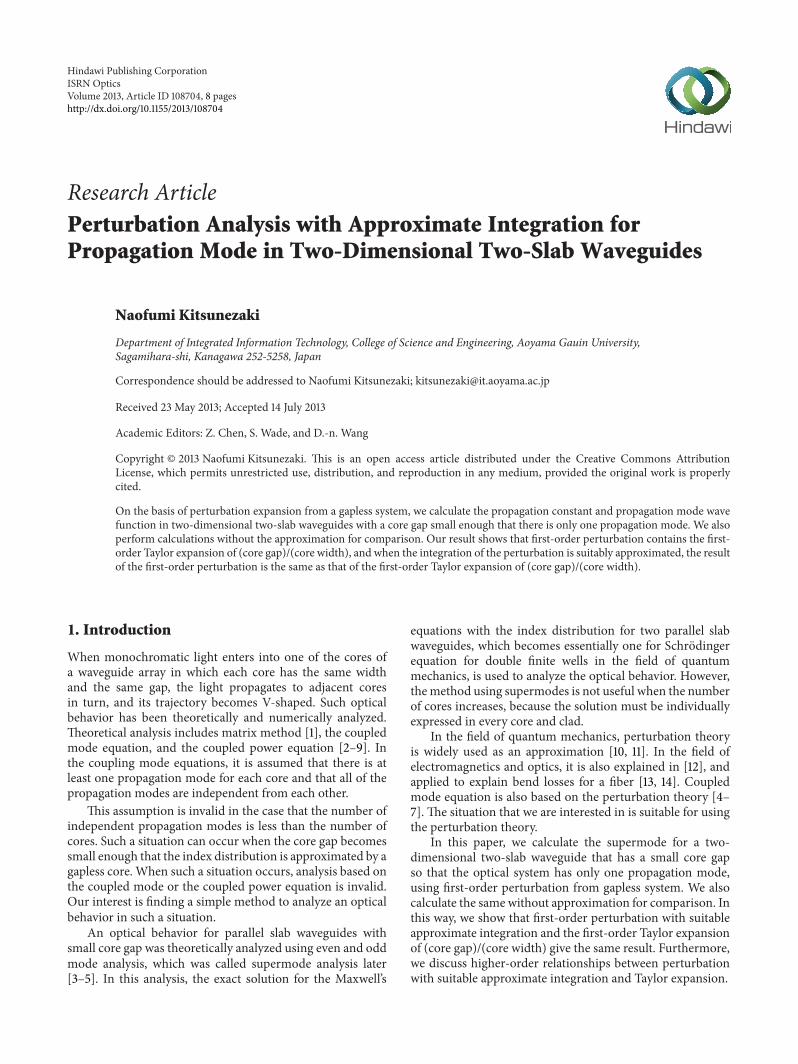
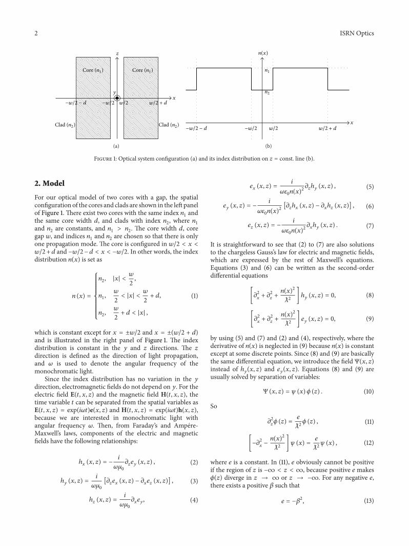
Figure 1 Optical system configuration (a) and its index distribution on 119911 = const line (b)
2 Model
For our optical model of two cores with a gap the spatialconfiguration of the cores and clads are shown in the left panelof Figure 1 There exist two cores with the same index 119899
1and
the same core width 119889 and clads with index 1198992 where 119899
1
and 1198992are constants and 119899
1gt 1198992 The core width 119889 core
gap 119908 and indices 1198991and 119899
2are chosen so that there is only
one propagation mode The core is configured in 1199082 lt 119909 lt
1199082+119889 and minus1199082minus119889 lt 119909 lt minus1199082 In other words the indexdistribution 119899(119909) is set as
119899 (119909) =
1198992 |119909| lt
119908
2
1198991
119908
2
lt |119909| lt
119908
2
+ 119889
1198992
119908
2
+ 119889 lt |119909|
(1)
which is constant except for 119909 = plusmn1199082 and 119909 = plusmn(1199082 + 119889)
and is illustrated in the right panel of Figure 1 The indexdistribution is constant in the 119910 and 119911 directions The 119911
direction is defined as the direction of light propagationand 120596 is used to denote the angular frequency of themonochromatic light
Since the index distribution has no variation in the 119910
direction electromagnetic fields do not depend on 119910 For theelectric field E(119905 119909 119911) and the magnetic field H(119905 119909 119911) thetime variable 119905 can be separated from the spatial variables asE(119905 119909 119911) = exp(119894120596119905)e(119909 119911) and H(119905 119909 119911) = exp(119894120596119905)h(119909 119911)because we are interested in monochromatic light withangular frequency 120596 Then from Faradayrsquos and Ampere-Maxwellrsquos laws components of the electric and magneticfields have the following relationships
ℎ119909(119909 119911) = minus
119894
1205961205830
120597119911119890119910(119909 119911) (2)
ℎ119910(119909 119911) =
119894
1205961205830
[120597119911119890119909(119909 119911) minus 120597
119909119890119911(119909 119911)] (3)
ℎ119911(119909 119911) =
119894
1205961205830
120597119909119890119910 (4)
119890119909(119909 119911) =
119894
1205961205760119899(119909)2120597119911ℎ119910(119909 119911) (5)
119890119910(119909 119911) = minus
119894
1205961205760119899(119909)2[120597119911ℎ119909(119909 119911) minus 120597
119909ℎ119911(119909 119911)] (6)
119890119911(119909 119911) = minus
119894
1205961205760119899(119909)2120597119909ℎ119910(119909 119911) (7)
It is straightforward to see that (2) to (7) are also solutionsto the chargeless Gaussrsquos law for electric and magnetic fieldswhich are expressed by the rest of Maxwellrsquos equationsEquations (3) and (6) can be written as the second-orderdifferential equations
[1205972
119909+ 1205972
119911+
119899(119909)2
1205822
] ℎ119910(119909 119911) = 0 (8)
[1205972
119909+ 1205972
119911+
119899(119909)2
1205822
] 119890119910(119909 119911) = 0 (9)
by using (5) and (7) and (2) and (4) respectively where thederivative of 119899(119909) is neglected in (9) because 119899(119909) is constantexcept at some discrete points Since (8) and (9) are basicallythe same differential equation we introduce the field Ψ(119909 119911)
instead of ℎ119910(119909 119911) and 119890
119910(119909 119911) Equations (8) and (9) are
usually solved by separation of variables
Ψ (119909 119911) = 120595 (119909) 120601 (119911) (10)
So
1205972
119911120601 (119911) =
119890
1205822120601 (119911) (11)
[minus1205972
119909minus
119899(119909)2
1205822
]120595 (119909) =
119890
1205822120595 (119909) (12)
where 119890 is a constant In (11) 119890 obviously cannot be positiveif the region of 119911 is minusinfin lt 119911 lt infin because positive 119890 makes120601(119911) diverge in 119911 rarr infin or 119911 rarr minusinfin For any negative 119890there exists a positive 120573 such that
119890 = minus1205732 (13)
ISRN Optics 3
where 120573 is the propagation constant and the solution of (11)represents propagation in the positive or negative 119911 directionwith 120573 = [minus119890]
12Equation (12) is essentially the one-dimensional
Schrodinger equation [10 11] which is an eigenfunctionproblem where 119890 is the eigenvalue and120595 is the eigenfunctionof the operator
minus1205972
119909minus
119899(119909)2
1205822
(14)
Equation (12) has nontrivial solutions for special values 119890
in minus1198992
1lt 119890 lt minus119899
2
2(propagation mode solution) and two
nontrivial solutions exist for each 119890 in minus1198992
2lt 119890 (radiation
mode solution)In the following section we solve (12) by using first-order
perturbation with a suitable approximation integration inorder to calculate the difference of its propagation constantand propagationmode solution from that of a gapless systemIn Section 4 we solve (12) without approximation in orderto obtain the first-order Taylor expansion of 119908119889 and thenwe compared the result with those obtained in Section 3Thefinal section is devoted to summary and discussion
3 Solution with First-Order Perturbation
To solve (12) we decompose the square of the index distribu-tionminus119899(119909)
2 into the square of the index distribution for119908 = 0
(minus1198990(119909)2) and the rest (minus119899
119901(119909)2) as
minus119899(119909)2= minus1198990(119909)2minus 119899119901(119909)2 (15)
where
1198990(119909) =
1198991
1003816100381610038161003816100381610038161003816
119909 minus
119908
2
1003816100381610038161003816100381610038161003816
lt 119889
1198992 119889 lt
1003816100381610038161003816100381610038161003816
119909 minus
119908
2
1003816100381610038161003816100381610038161003816
119899119901(119909) =
[1198992
1minus 1198992
2]
12
minus
119908
2
minus 119889 lt 119909 lt
119908
2
minus 119889
minus[1198992
1minus 1198992
2]
12
minus
119908
2
lt 119909 lt
119908
2
0 otherwise
(16)
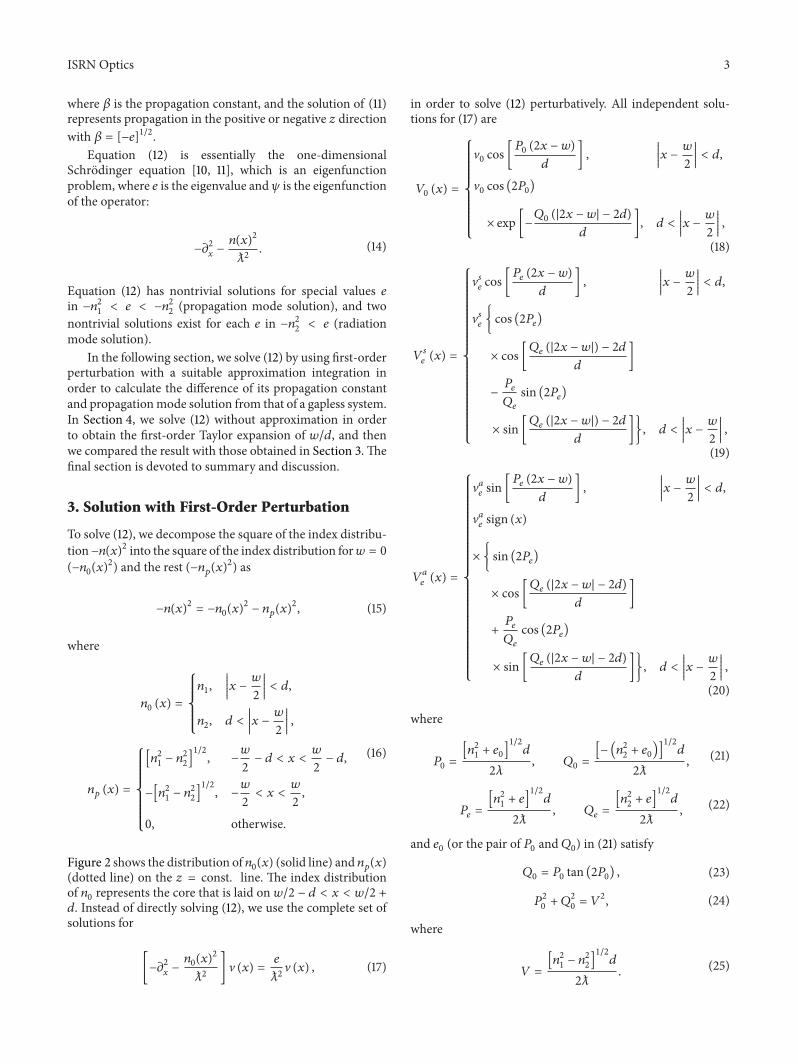
Figure 2 shows the distribution of 1198990(119909) (solid line) and 119899
119901(119909)
(dotted line) on the 119911 = const line The index distributionof 1198990represents the core that is laid on 1199082 minus 119889 lt 119909 lt 1199082 +
119889 Instead of directly solving (12) we use the complete set ofsolutions for
[minus1205972
119909minus
1198990(119909)2
1205822
] V (119909) =
119890
1205822V (119909) (17)
in order to solve (12) perturbatively All independent solu-tions for (17) are
1198810(119909) =
V0cos [
1198750(2119909 minus 119908)
119889
]
1003816100381610038161003816100381610038161003816
119909 minus
119908
2
1003816100381610038161003816100381610038161003816
lt 119889
V0cos (2119875
0)
times exp [minus
1198760(|2119909 minus 119908| minus 2119889)
119889
] 119889 lt
1003816100381610038161003816100381610038161003816
119909 minus
119908
2
1003816100381610038161003816100381610038161003816
(18)
119881119904
119890(119909) =
V119904119890cos [
119875119890(2119909 minus 119908)
119889
]
1003816100381610038161003816100381610038161003816
119909 minus
119908
2
1003816100381610038161003816100381610038161003816
lt 119889
V119904119890 cos (2119875
119890)
times cos [119876119890(|2119909 minus 119908|) minus 2119889
119889
]
minus
119875119890
119876119890
sin (2119875119890)
times sin [
119876119890(|2119909 minus 119908|) minus 2119889
119889
] 119889 lt
1003816100381610038161003816100381610038161003816
119909 minus
119908
2
1003816100381610038161003816100381610038161003816
(19)
119881119886
119890(119909) =
V119886119890sin [
119875119890(2119909 minus 119908)
119889
]
1003816100381610038161003816100381610038161003816
119909 minus
119908
2
1003816100381610038161003816100381610038161003816
lt 119889
V119886119890sign (119909)
times sin (2119875119890)
times cos [119876119890(|2119909 minus 119908| minus 2119889)
119889
]
+
119875119890
119876119890
cos (2119875119890)
times sin [
119876119890(|2119909 minus 119908| minus 2119889)
119889
] 119889 lt
1003816100381610038161003816100381610038161003816
119909 minus
119908
2
1003816100381610038161003816100381610038161003816
(20)
where
1198750=
[1198992
1+ 1198900]
12
119889
2120582
1198760=
[minus (1198992
2+ 1198900)]
12
119889
2120582
(21)
119875119890=
[1198992
1+ 119890]
12
119889
2120582
119876119890=
[1198992
2+ 119890]
12
119889
2120582
(22)
and 1198900(or the pair of 119875
0and 119876
0) in (21) satisfy
1198760= 1198750tan (2119875
0) (23)
1198752
0+ 1198762
0= 1198812 (24)
where
119881 =
[1198992
1minus 1198992
2]
12
119889
2120582
(25)
4 ISRN Optics
n2
n1
xw2 + dminusw2 minus d
minusw2 w2
n(x)
w2 minus d
radicn21minus n2
2
minusradicn21minus n2
2
Figure 2 Decomposed index distributions Solid line represents1198990(119909) and dotted line represents 119899
119901(119909)
In (22) 119890 is in the region
minus1198992
2lt 119890 lt 0 (26)
1198810represents the propagation mode and 119881
119904
119890and 119881
119886
119890
represent symmetric and antisymmetric radiation modesaccording to 119890 respectively For the reasons stated in theintroduction we are interested in the case that the propaga-tion mode of the optical system has only one independentmode Therefore we examine the case where the normalizedpropagation mode solution of (18) is 119881
0only
Here let us define the inner product of fields 119891 sdot 119892 as
119891 sdot 119892 =
1
119889
int
infin
minusinfin
119889119909119891 (119909) 119892 (119909) (27)
Then V0 V119904119890 and V119886
119890are defined so that 119881
0 119881119904119890 and 119881
119886
119890are
normalized to
1198810sdot 1198810= 1
119881119901
119890sdot 119881119902
119891= 120575119901119902120575 (119890 minus 119891)
(28)
where 119901 119902 isin 119904 119886 (note that 1198810 119881119904
119890and 119881
119886
119890can be
regarded as eigenfunctions of the eigenequation (17) andtheir eigenvalues are 119890
0 119890 and 119890 respectively In addition to
the relationships in (28) 1198810sdot 119881119904
119890= 0 and 119881
0sdot 119881119886
119890= 0 [10 11])
For instance V0is
V0= [
21198760
21198760+ 1
]
12
(29)
In perturbation theory the propagation mode solution for(12) is determined by using (18) to (20) which results in
[minus1205972
119909minus
1198990(119909)2
1205822
] minus
119899119901(119909)2
1205822
[1198810(119909) + Δ119881 (119909)]
=
1198900+ Δ119890
1205822
[1198810(119909) + Δ119881 (119909)]
(30)
The results of the first-order perturbation for Δ119890 and Δ119881 areas follows [10 11]
Δ119890 = minus1198810sdot (1198992
1199011198810) (31)
1198810sdot Δ119881 = 0 (32)
119881119901
119890sdot Δ119881 =
119881119901
119890sdot (1198992
1199011198810)
119890 minus 1198900
(33)
where
(1198992
1199011198810) (119909) = 119899
119901(119909)21198810(119909) (34)
In (33)119881119904119890sdot Δ119881 and119881
119886
119890sdot Δ119881mean the119881119904
119890and119881
119886
119890components
of Δ119881 respectively Note that for any field 119891(119909) the innerproduct with 119899
2
1199011198810is
119891 sdot (1198992
1199011198810) =
1198992
1minus 1198992
2
119889
[int
(1199082)minus119889
minus(1199082)minus119889
119889119909119891 (119909)1198810(119909)
minusint
1199082
minus(1199082)
119889119909119891 (119909)1198810(119909)]
(35)
= (1198992
1minus 1198992
2) [119891(
119908
2
minus 119889)1198810(
119908
2
minus 119889)
minus119891(
119908
2
)1198810(
119908
2
) ]
119908=0
119908
119889
+ 119900(
119908
119889
)
2
(36)
which means that it contains the first-order Taylor expansionof 119908119889 In the deformation from (35) to (36) we use theEuler method for the integration Using (18) through (20) weobtain the first-order Taylor expansion of119908119889 forΔ119890119881119904
119890sdotΔ119881
and 119881119886
119890sdot Δ119881 from (31) and (33) respectively as follows
Δ119890 = V20(1198992
1minus 1198992
2) [1 minus cos2 (2119875
0)]
=
21198760(1198992
1minus 1198992
2) sin2 (2119875
0)
21198760+ 1
119908
119889
(37)
119881119904
119890sdot Δ119881 = minusV
0V119890119904
(1198992
1minus 1198992
2) [1 minus cos (2119875
0) cos (2119875
119890)]
119890 minus 1198900
119908
119889
(38)
119881119886
119890sdot Δ119881 = minusV
0V119890119904
(1198992
1minus 1198992
2) sin (2119875
0) cos (2119875
119890)
119890 minus 1198900
119908
119889
(39)
ISRN Optics 5
4 Solution without Approximation
When the exact eigenvalue of the propagation mode of (12)is 119890119908 its eigenfunction is
119882(119909) =
1199080cosh (
2119876119908119909
119889
) |119909| lt
119908
2
1199080cosh (
119876119908119908
119889
)
times cos [119875119908(2 |119909| minus 119908)
119889
]
+
119876119908
119875119908
sinh(
119876119908119908
119889
)
times sin [
119875119908(2 |119909| minus 119908)
119889
]
119908
2
lt|119909|lt
119908
2
+119889
1199080[cosh (
119876119908119908
119889
) cos (2119875119908)
+
119876119908
119875119908
sinh(
119876119908119908
119889
)
times sin (2119875119908) ]
times exp [minus
119876119908(2 |119909| minus 2119889minus119908)
119889
]
119908
2
+ 119889 lt |119909|
(40)
where
119875119908
=
[1198992
1+ 119890119908]
12
119889
2120582
119876119908
=
[minus (1198992
2+ 119890119908)]
12
119889
2120582
(41)
119875119908and 119876
119908satisfy the relationships
119875119908[119875119908sin (2119875
119908) minus 119876119908cos (2119875
119908)]
= 1198812 exp(minus
119876119908119908
119889
) sinh(
119876119908119908
119889
) sin (2119875119908)
1198752
119908+ 1198762
119908= 1198812
(42)
such that 119882(119909) and its derivative are continuous for any 119909Note that 119882
0(119909) agrees with 119881
0(119909) in the limit of 119908119889 = 0
and 1199080becomes V
0when 119908119889 = 0 When 119908119889 = 0 the
relationships between 119882(119909) and Δ119881(119909) and between 119890119908and
Δ119890 become the following
119882(119909) = 1198810(119909) + Δ119881 (43)
119890119908
= 1198900+ Δ119890 (44)
Substituting (44) into (42) by using (41) and applying (23)we obtain
[21198750sin (2119875
0) + cos (2119875
0)] 1198812Δ119890
2 (1198992
1minus 1198992
2) sin (2119875
0) cos (2119875
0)
[1 + 119874 (Δ119890)]
= 11988121198760sin (2119875
0)
119908
119889
[1 + 119874(
119908
119889
Δ119890)]
(45)
Comparing the lowest order of Δ119890 and 119908119889 in (45) using(23) we obtain (37) from (45) Because of (13) the first-orderperturbation and the first-order Taylor expansion of119908119889 givethe same propagation constant for a two-core optical systemwith gap 119908
119881119904
119890sdot 119882 and 119881
119886
119890sdot 119882 are directly derived which results in
119881119904
119890sdot 1198820
= V0V119904119890(
119876119908[1 + cosh (2119875
119890119908119889)] sin (119876
119908119908119889) + 119875
119890sinh (2119875
119890119908119889) cos (119876
119908119908119889)
2 (1198752
119890+ 1198762
119908)
+
119875119908cosh (119876
119908119908119889) cos (2119875
119908) + 119876119908sinh (119876
119908119908119889) sin (2119875
119908)
119875119908(1198762
119890+ 1198762
119908)
times
[1 + 2 cos (2119876119890119908119889) minus exp (2119876
119908119908119889)] [119876
119908cos (2119875
119890) minus 119875119890sin (2119875
119890)]
2
+
[1198762
119890cos (2119875
119890) + 119875119890119876119908sin (2119875
119890)] sin (2119876
119890119908119889)
119876119890
minus
1
1198752
119890minus 1198752
119908
[119875119908cosh (
119876119908119908
119889
)(
[1 + cos (2119875119908119908119889)] sin (2119875
119908) cos (2119875
119890)
2
minus
sin (2119875119908119908119889) cos (2119875
119908) cos (2119875
119890)
2
6 ISRN Optics
minus
119875119890
119875119908
[1 + cos (2119875119908119908119889)] cos (2119875
119908) cos (2119875
119890)
2
+
sin (2119875119908119908119889) sin (2119875
119908) sin (2119875
119890)
2
minus sin(
2119875119890119908
119889
))
+ 119876119908sinh(
119876119908119908
119889
)
[1 + cos (2119875119890119908119889)] [1 minus cos (2119875
119908) cos (2119875
119890)]
2
minus
sin (2119875119908119908119889) sin (2119875
119908) sin (2119875
119890)
2
+ cos(2119875119890119908
119889
)
minus cos(2119875119908119908
119889
) minus
[1 + cos (2119875119908119908119889)] sin (2119875
119908) sin (2119875
119890)
2
+
sin (2119875119908119908119889) cos (2119875
119908) cos (2119875
119890)
2
]
minus (([119875119908sin(
2119875119908119908
119889
) minus 119876119890sin(
2119876119890119908
119889
)] cosh (
119876119908119908
119889
)
minus 119876119908[cos(
2119876119890119908
119889
) minus cos(2119875119908119908
119889
)] sinh(
119876119908119908
119889
) cos (2119875119908) cos (2119875
119890))
times (2 (1198762
119890minus 1198752
119908))
minus1
)
minus ((119875119890[sin(
2119875119908119908
119889
) +
119875119908
119876119890
sin(
2119876119890119908
119889
)] cosh (
119876119908119908
119889
)
minus
119876119908119875119890
119875119908
[cos(2119876119890119908
119889
) minus cos(2119875119908119908
119889
)] sinh(
119876119908119908
119889
) sin (2119875119908) sin (2119875
119890))
times (2 (1198762
119890minus 1198752
119908))
minus1
)
minus ((119876119908[sin(
2119875119908119908
119889
) +
119876119890
119875119908
sin(
2119876119890119908
119889
)] sinh(
119876119908119908
119889
)
+ [cos(2119876119890119908
119889
) minus cos(2119875119908119908
119889
)] cosh (
119876119908119908
119889
) sin (2119875119908) cos (2119875
119890))
times (2 (1198762
119890minus 1198752
119908))
minus1
)
+ ((119875119890119875119908
1
119875119908
[sin(
2119875119908119908
119889
) +
1
119876119890
sin(
2119876119890119908
119889
)] sinh(
119876119908119908
119889
)
+ 119875119890[cos(
2119876119890119908
119889
) minus cos(2119875119908119908
119889
)] cosh (
119876119908119908
119889
) cos (2119875119908) sin (2119875
119890))
times (2 (1198762
119890minus 1198752
119908))
minus1
))
119881119886
119890sdot 1198820
= V119886119890V0(minus
119875119890[1 minus cos (2119875
119890119908119889)] cosh (119876
119908119908119889) + 119876
119908sinh (119876
119908119908119889) sin (2119875
119890119908119889)
2 (1198752
119890+ 1198762
119908)
+
119875119908cosh (119876
119908119908119889) cos (2119875
119908) + 119876119908sinh (119876
119908119908119889) sin (2119875
119908)
119875119908(1198762
119890+ 1198762
119908)
times
[1 minus cos (2119876119890119908119889)] [119876
119908sin (2119875
119890) + 119875119890cos (2119875
119890)]
2
+
[1198762
119890sin (2119875
119890) minus 119875119890119876119908cos (2119875
119890)] sin (2119875
119890119908119889)
4119876119890
ISRN Optics 7
+
1 minus cos (2119875119890119908119889)
2
119875119908cosh (119876
119908119908119889) 119875
119890[1 minus cos (2119875
119908) cos (2119875
119890)] minus 119875
119908sin (2119875
119908) sin (2119875
119890)
119875119908(1198752
119890minus 1198752
119908)
+
1 minus cos (2119875119890119908119889)
2
119876119908sinh (119876
119908119908119889) [119875
119890cos (2119875
119908) sin (2119875
119890) minus 119875119908sin (2119875
119908) cos (2119875
119890)]
119875119908(1198752
119890minus 1198752
119908)
+
sin (2119875119890119908119889)
2
119875119908cosh (119876
119908119908119889) [119875
119908sin (2119875
119908) cos (2119875
119890) minus 119875119890cos (2119875
119908) sin (2119875
119890)]
119875119908(1198752
119890minus 1198752
119908)
+
sin (2119875119890119908119889)
2
119876119908sinh (119876
119908119908119889) 119875
119908[1 minus cos (2119875
119908) cos (2119875
119890)] minus 119875
119890sin (2119875
119908) sin (2119875
119890)
119875119908(1198752
119890minus 1198752
119908)
minus ((cosh (
119876119908119908
119889
)119875119890[cos (2119875
119908) cos (2119875
119890) minus cos(
2119875119908(119889 minus 119908)
119889
) cos(2119875119890(119889 minus 119908)
119889
)]
+ 119875119908
[sin (2119875119908) sin (2119875
119890) minus sin(
2119875119908(119889 minus 119908)
119889
) sin(
2119875119890(119889 minus 119908)
119889
)])
times (2 (1198752
119890minus 1198752
119908))
minus1
)
+ ((119876119908sinh(
119876119908119908
119889
)119875119890[cos (2119875
119908) sin (2119875
119890) minus cos(
2119875119908(119889 minus 119908)
119889
) sin(
2119875119890(119889 minus 119908)
119889
)]
minus 119875119908
[sin (2119875119908) cos (2119875
119890) minus sin(
2119875119908(119889 minus 119908)
119889
) cos(21198750(119889 minus 119908)
119889
)])
times (2119875119908(1198752
119890minus 1198752
119908))
minus1
)
+ ((sinh(
119876119908119908
119889
)119875119890[sin(
2119875119908119908
119889
) +
119875119908
119876119890
sin(
2119876119890119908
119889
)] cos (2119875119908) cos (2119875
119890)
minus
119876119908
119875119908
[119875119908sin(
2119875119908119908
119889
) + 119876119890sin(
2119876119890119908
119889
)] sin (2119875119908) sin (2119875
119890))
times (2 (1198762
119890minus 1198752
119908))
minus1
)
+ ((cosh (
119876119908119908
119889
)119876119890[119875119908sin(
2119875119908119908
119889
) + 119876119890sin(
2119876119890119908
119889
)] cos (2119875119908) sin (2119875
119890)
minus 119875119890[119876119890sin(
2119875119908119908
119889
) + 119875119908sin(
2119876119890119908
119889
)] sin (2119875119908) cos (2119875
119890)) times (2119876
119890(1198762
119890minus 1198752
119908))
minus1
) )
(46)
From (46) we obtain the first-order Taylor expansion of119908119889
of 119881119904
119890sdot 119882 and 119881
119886
119890sdot 119882 after a straightforward but lengthy
calculation
119881119904
119890sdot 119882 = minusV
0V119904119890
(1198992
1minus 1198992
2) [1 minus cos (2119875
0) cos (2119875
119890)]
119890 minus 1198900
119908
119889
(47)
119881119886
119890sdot 119882 = minusV
0V119886119890
(1198992
1minus 1198992
2) sin (2119875
0) cos (2119875
119890)
119890 minus 1198900
119908
119889
(48)
119881119904
119890sdotΔ119881 and119881
119886
119890sdotΔ119881 are equal to119881
119904
119890sdot119882 and119881
119886
119890sdot119882 respectively
because of (32) and (43) As shown above (38) and (39)completely coincide with (47) and (48) respectively
5 Conclusion and Discussion
We have shown that in a two-dimensional two-slab waveg-uide system that has a small core gap so that the optical systemhas only one propagation mode the supermode and itspropagation constant calculated by first-order perturbationby the Euler method and the first-order Taylor expansion of119908119889 for the exact solution give the same result up to (119908119889)
1
orderAs for higher-order perturbation the correction of 119890
119908by
second-order perturbation is given by [10]
sum
119901isin119904119886
int
0
minus1198992
2
119889119890120588 (119890)
10038161003816100381610038161003816119881119901
119890sdot (1198992
21198810)
10038161003816100381610038161003816
2
119890 minus 1198900
(49)
8 ISRN Optics
where 120588(119890) represents mode density function and the correc-tion of 119881119901
119890sdot 119882 is
sum
119902isin119904119886
int
0
minus1198992
2
119889119891
119881119901
119890sdot (1198992
2119881119902
119891)119881119902
119891sdot (1198992
21198810)
(119890 minus 1198900) (119891 minus 119890
0)
minus
119881119901
119890sdot (1198992
21198810)1198810sdot (1198992
21198810)
(119890 minus 1198900)2
(50)
The lowest order of119908119889 for (49) and (50) is119874(119908119889)2 because
of the argument given in Section 3 Therefore second-orderperturbation with the Euler method is a part of the second-order Taylor expansion of 119908119889 As shown in (36) the first-order perturbation can include the second order of 119908119889To obtain the second order of 119908119889 from the first-orderperturbation integration over minus1199082 lt 119909 lt 1199082 minus 119889
and minus1199082 lt 119909 lt 1199082 in the perturbation must beapproximated by the trapezoidal rule instead of the Eulermethod Thus first-order perturbation by the trapezoidalrule in combination with a second-order perturbation by theEuler method gives the same result as the exact calculationgiven by the second-order Taylor expansion of 119908119889 In asimilar way the 119899th-order coefficient of the Taylor expansionof 119908119889 is obtained from all orders of perturbation less thanthe 119899th order In each order of perturbation exact integrationover minus1199082 minus 119889 lt 119909 lt 1199082 minus 119889 and minus1199082 lt 119909 lt 1199082 is notnecessary instead a suitable approximation of integrationincluding the (119908119889)
119899 order term is necessary Thus whenan optical system has two cores with a small gap it can beanalyzed by perturbation using modes of an optical systemwith a gapless core with twice the width
Obtaining the exact solution becomes time consuming asthe number of cores increases Even in such situations per-turbation analysis can be executed easilyHence perturbationanalysis using suitable approximate integration is a promisingcandidate for approximation in the region 119908119889 ≪ 1 whenthe coupledmode or power mode equation is invalid because119908119889 is very small
Acknowledgment
The authors thank all members of the Tobe Laboratory in theDepartment of Integrated Information Technology Collegeof Science and Engineering Aoyama Gakuin University forcomments and discussion
References
[1] A Ghatak and V Lakshminarayanan ldquoPropagation character-istics of planar waveguidesrdquo in Optical Waveguides fromTheoryto Applied Technologies M L Calvo and V LakshminarayananEds p CRC press New York NY USA 2007
[2] A Yariv ldquoCoupling-mode theory for guided-wave opticsrdquo IEEEJournal of Quantum Electronics vol QE-9 no 9 pp 919ndash9331973
[3] Y Suematsu and K Kishino ldquoCoupling coefficient in stronglycoupled dielectric waveguidesrdquo Radio Science vol 12 no 4 pp587ndash592 1977
[4] A Hardy and W Streifer ldquoCoupled mode theory of parallelwaveguidesrdquo Journal of Lightwave Technology vol 3 no 5 pp1135ndash1146 1985
[5] A Hardy and W Streifer ldquoCoupled modes of multiwaveguidesystem and phased arraysrdquo Journal of Lightwave Technology vol4 no 1 pp 90ndash99 1986
[6] H A Haus W P Huang S Kawakami and N A WhitakerldquoCoupled-mode theory of optical waveguidesrdquo Journal of Light-wave Technology vol 5 no 1 pp 16ndash23 1987
[7] K Yasumoto ldquoCoupled-mode formulation of parallel dielectricwaveguides using singular perturbation techniquerdquoMicrowaveand Optical Technology Letters vol 4 no 11 pp 486ndash491 1991
[8] H Yoshida K Hidaka and N Tsukada ldquoProposal of opticalwaveguide array beam splitter andMach-Zehnder optical inter-ferometerrdquo IEICE Technical Report OCS2010-36 2010
[9] A Komiyama ldquoEnergy conservation in a waveguide systemwith an imperfection corerdquoThe Papers of Technical Meeting onElectromagnetic Theory IEEJ EMT-11-131 2011
[10] L I ShiffQuantumMechanics Mc-Graw Hill Singapore 1969[11] W Greiner Quantum MechanicsmdashAn Introduction Springer
Berlin Germany 1989[12] R F HarringtonTime-Harmonic Electromagnetic FieldsWiley-
Interscience New York NY USA 2001[13] C Vassallo ldquoPerturbation of a LP mode of an optical fibre by a
quasi-degenerate field a simple formulardquoOptical and QuantumElectronics vol 17 no 3 pp 201ndash205 1985
[14] QWang G Farrell and T Freir ldquoTheoretical and experimentalinvestigations of macro-bend Losses for standard single modefibersrdquo Optics Express vol 13 no 12 pp 4476ndash4484 2005
Submit your manuscripts athttpwwwhindawicom
Hindawi Publishing Corporationhttpwwwhindawicom Volume 2014
High Energy PhysicsAdvances in
The Scientific World JournalHindawi Publishing Corporation httpwwwhindawicom Volume 2014
Hindawi Publishing Corporationhttpwwwhindawicom Volume 2014
FluidsJournal of
Atomic and Molecular Physics
Journal of
Hindawi Publishing Corporationhttpwwwhindawicom Volume 2014
Hindawi Publishing Corporationhttpwwwhindawicom Volume 2014
Advances in Condensed Matter Physics
OpticsInternational Journal of
Hindawi Publishing Corporationhttpwwwhindawicom Volume 2014
Hindawi Publishing Corporationhttpwwwhindawicom Volume 2014
AstronomyAdvances in
International Journal of
Hindawi Publishing Corporationhttpwwwhindawicom Volume 2014
Superconductivity
Hindawi Publishing Corporationhttpwwwhindawicom Volume 2014
Statistical MechanicsInternational Journal of
Hindawi Publishing Corporationhttpwwwhindawicom Volume 2014
GravityJournal of
Hindawi Publishing Corporationhttpwwwhindawicom Volume 2014
AstrophysicsJournal of
Hindawi Publishing Corporationhttpwwwhindawicom Volume 2014
Physics Research International
Hindawi Publishing Corporationhttpwwwhindawicom Volume 2014
Solid State PhysicsJournal of
Computational Methods in Physics
Journal of
Hindawi Publishing Corporationhttpwwwhindawicom Volume 2014
Hindawi Publishing Corporationhttpwwwhindawicom Volume 2014
Soft MatterJournal of
Hindawi Publishing Corporationhttpwwwhindawicom
AerodynamicsJournal of
Volume 2014
Hindawi Publishing Corporationhttpwwwhindawicom Volume 2014
PhotonicsJournal of
Hindawi Publishing Corporationhttpwwwhindawicom Volume 2014
Journal of
Biophysics
Hindawi Publishing Corporationhttpwwwhindawicom Volume 2014
ThermodynamicsJournal of
2 ISRN Optics
Clad (n2) Clad (n2)
x
z
w2 + dminusw2 minus d minusw2 w2
Core (n1) Core (n1)
y
(a)
n2
n1
xw2 + dminusw2 minus d minusw2 w2
n(x)
(b)
Figure 1 Optical system configuration (a) and its index distribution on 119911 = const line (b)
2 Model
For our optical model of two cores with a gap the spatialconfiguration of the cores and clads are shown in the left panelof Figure 1 There exist two cores with the same index 119899
1and
the same core width 119889 and clads with index 1198992 where 119899
1
and 1198992are constants and 119899
1gt 1198992 The core width 119889 core
gap 119908 and indices 1198991and 119899
2are chosen so that there is only
one propagation mode The core is configured in 1199082 lt 119909 lt
1199082+119889 and minus1199082minus119889 lt 119909 lt minus1199082 In other words the indexdistribution 119899(119909) is set as
119899 (119909) =
1198992 |119909| lt
119908
2
1198991
119908
2
lt |119909| lt
119908
2
+ 119889
1198992
119908
2
+ 119889 lt |119909|
(1)
which is constant except for 119909 = plusmn1199082 and 119909 = plusmn(1199082 + 119889)
and is illustrated in the right panel of Figure 1 The indexdistribution is constant in the 119910 and 119911 directions The 119911
direction is defined as the direction of light propagationand 120596 is used to denote the angular frequency of themonochromatic light
Since the index distribution has no variation in the 119910
direction electromagnetic fields do not depend on 119910 For theelectric field E(119905 119909 119911) and the magnetic field H(119905 119909 119911) thetime variable 119905 can be separated from the spatial variables asE(119905 119909 119911) = exp(119894120596119905)e(119909 119911) and H(119905 119909 119911) = exp(119894120596119905)h(119909 119911)because we are interested in monochromatic light withangular frequency 120596 Then from Faradayrsquos and Ampere-Maxwellrsquos laws components of the electric and magneticfields have the following relationships
ℎ119909(119909 119911) = minus
119894
1205961205830
120597119911119890119910(119909 119911) (2)
ℎ119910(119909 119911) =
119894
1205961205830
[120597119911119890119909(119909 119911) minus 120597
119909119890119911(119909 119911)] (3)
ℎ119911(119909 119911) =
119894
1205961205830
120597119909119890119910 (4)
119890119909(119909 119911) =
119894
1205961205760119899(119909)2120597119911ℎ119910(119909 119911) (5)
119890119910(119909 119911) = minus
119894
1205961205760119899(119909)2[120597119911ℎ119909(119909 119911) minus 120597
119909ℎ119911(119909 119911)] (6)
119890119911(119909 119911) = minus
119894
1205961205760119899(119909)2120597119909ℎ119910(119909 119911) (7)
It is straightforward to see that (2) to (7) are also solutionsto the chargeless Gaussrsquos law for electric and magnetic fieldswhich are expressed by the rest of Maxwellrsquos equationsEquations (3) and (6) can be written as the second-orderdifferential equations
[1205972
119909+ 1205972
119911+
119899(119909)2
1205822
] ℎ119910(119909 119911) = 0 (8)
[1205972
119909+ 1205972
119911+
119899(119909)2
1205822
] 119890119910(119909 119911) = 0 (9)
by using (5) and (7) and (2) and (4) respectively where thederivative of 119899(119909) is neglected in (9) because 119899(119909) is constantexcept at some discrete points Since (8) and (9) are basicallythe same differential equation we introduce the field Ψ(119909 119911)
instead of ℎ119910(119909 119911) and 119890
119910(119909 119911) Equations (8) and (9) are
usually solved by separation of variables
Ψ (119909 119911) = 120595 (119909) 120601 (119911) (10)
So
1205972
119911120601 (119911) =
119890
1205822120601 (119911) (11)
[minus1205972
119909minus
119899(119909)2
1205822
]120595 (119909) =
119890
1205822120595 (119909) (12)
where 119890 is a constant In (11) 119890 obviously cannot be positiveif the region of 119911 is minusinfin lt 119911 lt infin because positive 119890 makes120601(119911) diverge in 119911 rarr infin or 119911 rarr minusinfin For any negative 119890there exists a positive 120573 such that
119890 = minus1205732 (13)
ISRN Optics 3
where 120573 is the propagation constant and the solution of (11)represents propagation in the positive or negative 119911 directionwith 120573 = [minus119890]
12Equation (12) is essentially the one-dimensional
Schrodinger equation [10 11] which is an eigenfunctionproblem where 119890 is the eigenvalue and120595 is the eigenfunctionof the operator
minus1205972
119909minus
119899(119909)2
1205822
(14)
Equation (12) has nontrivial solutions for special values 119890
in minus1198992
1lt 119890 lt minus119899
2
2(propagation mode solution) and two
nontrivial solutions exist for each 119890 in minus1198992
2lt 119890 (radiation
mode solution)In the following section we solve (12) by using first-order
perturbation with a suitable approximation integration inorder to calculate the difference of its propagation constantand propagationmode solution from that of a gapless systemIn Section 4 we solve (12) without approximation in orderto obtain the first-order Taylor expansion of 119908119889 and thenwe compared the result with those obtained in Section 3Thefinal section is devoted to summary and discussion
3 Solution with First-Order Perturbation
To solve (12) we decompose the square of the index distribu-tionminus119899(119909)
2 into the square of the index distribution for119908 = 0
(minus1198990(119909)2) and the rest (minus119899
119901(119909)2) as
minus119899(119909)2= minus1198990(119909)2minus 119899119901(119909)2 (15)
where
1198990(119909) =
1198991
1003816100381610038161003816100381610038161003816
119909 minus
119908
2
1003816100381610038161003816100381610038161003816
lt 119889
1198992 119889 lt
1003816100381610038161003816100381610038161003816
119909 minus
119908
2
1003816100381610038161003816100381610038161003816
119899119901(119909) =
[1198992
1minus 1198992
2]
12
minus
119908
2
minus 119889 lt 119909 lt
119908
2
minus 119889
minus[1198992
1minus 1198992
2]
12
minus
119908
2
lt 119909 lt
119908
2
0 otherwise
(16)
Figure 2 shows the distribution of 1198990(119909) (solid line) and 119899
119901(119909)
(dotted line) on the 119911 = const line The index distributionof 1198990represents the core that is laid on 1199082 minus 119889 lt 119909 lt 1199082 +
119889 Instead of directly solving (12) we use the complete set ofsolutions for
[minus1205972
119909minus
1198990(119909)2
1205822
] V (119909) =
119890
1205822V (119909) (17)
in order to solve (12) perturbatively All independent solu-tions for (17) are
1198810(119909) =
V0cos [
1198750(2119909 minus 119908)
119889
]
1003816100381610038161003816100381610038161003816
119909 minus
119908
2
1003816100381610038161003816100381610038161003816
lt 119889
V0cos (2119875
0)
times exp [minus
1198760(|2119909 minus 119908| minus 2119889)
119889
] 119889 lt
1003816100381610038161003816100381610038161003816
119909 minus
119908
2
1003816100381610038161003816100381610038161003816
(18)
119881119904
119890(119909) =
V119904119890cos [
119875119890(2119909 minus 119908)
119889
]
1003816100381610038161003816100381610038161003816
119909 minus
119908
2
1003816100381610038161003816100381610038161003816
lt 119889
V119904119890 cos (2119875
119890)
times cos [119876119890(|2119909 minus 119908|) minus 2119889
119889
]
minus
119875119890
119876119890
sin (2119875119890)
times sin [
119876119890(|2119909 minus 119908|) minus 2119889
119889
] 119889 lt
1003816100381610038161003816100381610038161003816
119909 minus
119908
2
1003816100381610038161003816100381610038161003816
(19)
119881119886
119890(119909) =
V119886119890sin [
119875119890(2119909 minus 119908)
119889
]
1003816100381610038161003816100381610038161003816
119909 minus
119908
2
1003816100381610038161003816100381610038161003816
lt 119889
V119886119890sign (119909)
times sin (2119875119890)
times cos [119876119890(|2119909 minus 119908| minus 2119889)
119889
]
+
119875119890
119876119890
cos (2119875119890)
times sin [
119876119890(|2119909 minus 119908| minus 2119889)
119889
] 119889 lt
1003816100381610038161003816100381610038161003816
119909 minus
119908
2
1003816100381610038161003816100381610038161003816
(20)
where
1198750=
[1198992
1+ 1198900]
12
119889
2120582
1198760=
[minus (1198992
2+ 1198900)]
12
119889
2120582
(21)
119875119890=
[1198992
1+ 119890]
12
119889
2120582
119876119890=
[1198992
2+ 119890]
12
119889
2120582
(22)
and 1198900(or the pair of 119875
0and 119876
0) in (21) satisfy
1198760= 1198750tan (2119875
0) (23)
1198752
0+ 1198762
0= 1198812 (24)
where
119881 =
[1198992
1minus 1198992
2]
12
119889
2120582
(25)
4 ISRN Optics
n2
n1
xw2 + dminusw2 minus d
minusw2 w2
n(x)
w2 minus d
radicn21minus n2
2
minusradicn21minus n2
2
Figure 2 Decomposed index distributions Solid line represents1198990(119909) and dotted line represents 119899
119901(119909)
In (22) 119890 is in the region
minus1198992
2lt 119890 lt 0 (26)
1198810represents the propagation mode and 119881
119904
119890and 119881
119886
119890
represent symmetric and antisymmetric radiation modesaccording to 119890 respectively For the reasons stated in theintroduction we are interested in the case that the propaga-tion mode of the optical system has only one independentmode Therefore we examine the case where the normalizedpropagation mode solution of (18) is 119881
0only
Here let us define the inner product of fields 119891 sdot 119892 as
119891 sdot 119892 =
1
119889
int
infin
minusinfin
119889119909119891 (119909) 119892 (119909) (27)
Then V0 V119904119890 and V119886
119890are defined so that 119881
0 119881119904119890 and 119881
119886
119890are
normalized to
1198810sdot 1198810= 1
119881119901
119890sdot 119881119902
119891= 120575119901119902120575 (119890 minus 119891)
(28)
where 119901 119902 isin 119904 119886 (note that 1198810 119881119904
119890and 119881
119886
119890can be
regarded as eigenfunctions of the eigenequation (17) andtheir eigenvalues are 119890
0 119890 and 119890 respectively In addition to
the relationships in (28) 1198810sdot 119881119904
119890= 0 and 119881
0sdot 119881119886
119890= 0 [10 11])
For instance V0is
V0= [
21198760
21198760+ 1
]
12
(29)
In perturbation theory the propagation mode solution for(12) is determined by using (18) to (20) which results in
[minus1205972
119909minus
1198990(119909)2
1205822
] minus
119899119901(119909)2
1205822
[1198810(119909) + Δ119881 (119909)]
=
1198900+ Δ119890
1205822
[1198810(119909) + Δ119881 (119909)]
(30)
The results of the first-order perturbation for Δ119890 and Δ119881 areas follows [10 11]
Δ119890 = minus1198810sdot (1198992
1199011198810) (31)
1198810sdot Δ119881 = 0 (32)
119881119901
119890sdot Δ119881 =
119881119901
119890sdot (1198992
1199011198810)
119890 minus 1198900
(33)
where
(1198992
1199011198810) (119909) = 119899
119901(119909)21198810(119909) (34)
In (33)119881119904119890sdot Δ119881 and119881
119886
119890sdot Δ119881mean the119881119904
119890and119881
119886
119890components
of Δ119881 respectively Note that for any field 119891(119909) the innerproduct with 119899
2
1199011198810is
119891 sdot (1198992
1199011198810) =
1198992
1minus 1198992
2
119889
[int
(1199082)minus119889
minus(1199082)minus119889
119889119909119891 (119909)1198810(119909)
minusint
1199082
minus(1199082)
119889119909119891 (119909)1198810(119909)]
(35)
= (1198992
1minus 1198992
2) [119891(
119908
2
minus 119889)1198810(
119908
2
minus 119889)
minus119891(
119908
2
)1198810(
119908
2
) ]
119908=0
119908
119889
+ 119900(
119908
119889
)
2
(36)
which means that it contains the first-order Taylor expansionof 119908119889 In the deformation from (35) to (36) we use theEuler method for the integration Using (18) through (20) weobtain the first-order Taylor expansion of119908119889 forΔ119890119881119904
119890sdotΔ119881
and 119881119886
119890sdot Δ119881 from (31) and (33) respectively as follows
Δ119890 = V20(1198992
1minus 1198992
2) [1 minus cos2 (2119875
0)]
=
21198760(1198992
1minus 1198992
2) sin2 (2119875
0)
21198760+ 1
119908
119889
(37)
119881119904
119890sdot Δ119881 = minusV
0V119890119904
(1198992
1minus 1198992
2) [1 minus cos (2119875
0) cos (2119875
119890)]
119890 minus 1198900
119908
119889
(38)
119881119886
119890sdot Δ119881 = minusV
0V119890119904
(1198992
1minus 1198992
2) sin (2119875
0) cos (2119875
119890)
119890 minus 1198900
119908
119889
(39)
ISRN Optics 5
4 Solution without Approximation
When the exact eigenvalue of the propagation mode of (12)is 119890119908 its eigenfunction is
119882(119909) =
1199080cosh (
2119876119908119909
119889
) |119909| lt
119908
2
1199080cosh (
119876119908119908
119889
)
times cos [119875119908(2 |119909| minus 119908)
119889
]
+
119876119908
119875119908
sinh(
119876119908119908
119889
)
times sin [
119875119908(2 |119909| minus 119908)
119889
]
119908
2
lt|119909|lt
119908
2
+119889
1199080[cosh (
119876119908119908
119889
) cos (2119875119908)
+
119876119908
119875119908
sinh(
119876119908119908
119889
)
times sin (2119875119908) ]
times exp [minus
119876119908(2 |119909| minus 2119889minus119908)
119889
]
119908
2
+ 119889 lt |119909|
(40)
where
119875119908
=
[1198992
1+ 119890119908]
12
119889
2120582
119876119908
=
[minus (1198992
2+ 119890119908)]
12
119889
2120582
(41)
119875119908and 119876
119908satisfy the relationships
119875119908[119875119908sin (2119875
119908) minus 119876119908cos (2119875
119908)]
= 1198812 exp(minus
119876119908119908
119889
) sinh(
119876119908119908
119889
) sin (2119875119908)
1198752
119908+ 1198762
119908= 1198812
(42)
such that 119882(119909) and its derivative are continuous for any 119909Note that 119882
0(119909) agrees with 119881
0(119909) in the limit of 119908119889 = 0
and 1199080becomes V
0when 119908119889 = 0 When 119908119889 = 0 the
relationships between 119882(119909) and Δ119881(119909) and between 119890119908and
Δ119890 become the following
119882(119909) = 1198810(119909) + Δ119881 (43)
119890119908
= 1198900+ Δ119890 (44)
Substituting (44) into (42) by using (41) and applying (23)we obtain
[21198750sin (2119875
0) + cos (2119875
0)] 1198812Δ119890
2 (1198992
1minus 1198992
2) sin (2119875
0) cos (2119875
0)
[1 + 119874 (Δ119890)]
= 11988121198760sin (2119875
0)
119908
119889
[1 + 119874(
119908
119889
Δ119890)]
(45)
Comparing the lowest order of Δ119890 and 119908119889 in (45) using(23) we obtain (37) from (45) Because of (13) the first-orderperturbation and the first-order Taylor expansion of119908119889 givethe same propagation constant for a two-core optical systemwith gap 119908
119881119904
119890sdot 119882 and 119881
119886
119890sdot 119882 are directly derived which results in
119881119904
119890sdot 1198820
= V0V119904119890(
119876119908[1 + cosh (2119875
119890119908119889)] sin (119876
119908119908119889) + 119875
119890sinh (2119875
119890119908119889) cos (119876
119908119908119889)
2 (1198752
119890+ 1198762
119908)
+
119875119908cosh (119876
119908119908119889) cos (2119875
119908) + 119876119908sinh (119876
119908119908119889) sin (2119875
119908)
119875119908(1198762
119890+ 1198762
119908)
times
[1 + 2 cos (2119876119890119908119889) minus exp (2119876
119908119908119889)] [119876
119908cos (2119875
119890) minus 119875119890sin (2119875
119890)]
2
+
[1198762
119890cos (2119875
119890) + 119875119890119876119908sin (2119875
119890)] sin (2119876
119890119908119889)
119876119890
minus
1
1198752
119890minus 1198752
119908
[119875119908cosh (
119876119908119908
119889
)(
[1 + cos (2119875119908119908119889)] sin (2119875
119908) cos (2119875
119890)
2
minus
sin (2119875119908119908119889) cos (2119875
119908) cos (2119875
119890)
2
6 ISRN Optics
minus
119875119890
119875119908
[1 + cos (2119875119908119908119889)] cos (2119875
119908) cos (2119875
119890)
2
+
sin (2119875119908119908119889) sin (2119875
119908) sin (2119875
119890)
2
minus sin(
2119875119890119908
119889
))
+ 119876119908sinh(
119876119908119908
119889
)
[1 + cos (2119875119890119908119889)] [1 minus cos (2119875
119908) cos (2119875
119890)]
2
minus
sin (2119875119908119908119889) sin (2119875
119908) sin (2119875
119890)
2
+ cos(2119875119890119908
119889
)
minus cos(2119875119908119908
119889
) minus
[1 + cos (2119875119908119908119889)] sin (2119875
119908) sin (2119875
119890)
2
+
sin (2119875119908119908119889) cos (2119875
119908) cos (2119875
119890)
2
]
minus (([119875119908sin(
2119875119908119908
119889
) minus 119876119890sin(
2119876119890119908
119889
)] cosh (
119876119908119908
119889
)
minus 119876119908[cos(
2119876119890119908
119889
) minus cos(2119875119908119908
119889
)] sinh(
119876119908119908
119889
) cos (2119875119908) cos (2119875
119890))
times (2 (1198762
119890minus 1198752
119908))
minus1
)
minus ((119875119890[sin(
2119875119908119908
119889
) +
119875119908
119876119890
sin(
2119876119890119908
119889
)] cosh (
119876119908119908
119889
)
minus
119876119908119875119890
119875119908
[cos(2119876119890119908
119889
) minus cos(2119875119908119908
119889
)] sinh(
119876119908119908
119889
) sin (2119875119908) sin (2119875
119890))
times (2 (1198762
119890minus 1198752
119908))
minus1
)
minus ((119876119908[sin(
2119875119908119908
119889
) +
119876119890
119875119908
sin(
2119876119890119908
119889
)] sinh(
119876119908119908
119889
)
+ [cos(2119876119890119908
119889
) minus cos(2119875119908119908
119889
)] cosh (
119876119908119908
119889
) sin (2119875119908) cos (2119875
119890))
times (2 (1198762
119890minus 1198752
119908))
minus1
)
+ ((119875119890119875119908
1
119875119908
[sin(
2119875119908119908
119889
) +
1
119876119890
sin(
2119876119890119908
119889
)] sinh(
119876119908119908
119889
)
+ 119875119890[cos(
2119876119890119908
119889
) minus cos(2119875119908119908
119889
)] cosh (
119876119908119908
119889
) cos (2119875119908) sin (2119875
119890))
times (2 (1198762
119890minus 1198752
119908))
minus1
))
119881119886
119890sdot 1198820
= V119886119890V0(minus
119875119890[1 minus cos (2119875
119890119908119889)] cosh (119876
119908119908119889) + 119876
119908sinh (119876
119908119908119889) sin (2119875
119890119908119889)
2 (1198752
119890+ 1198762
119908)
+
119875119908cosh (119876
119908119908119889) cos (2119875
119908) + 119876119908sinh (119876
119908119908119889) sin (2119875
119908)
119875119908(1198762
119890+ 1198762
119908)
times
[1 minus cos (2119876119890119908119889)] [119876
119908sin (2119875
119890) + 119875119890cos (2119875
119890)]
2
+
[1198762
119890sin (2119875
119890) minus 119875119890119876119908cos (2119875
119890)] sin (2119875
119890119908119889)
4119876119890
ISRN Optics 7
+
1 minus cos (2119875119890119908119889)
2
119875119908cosh (119876
119908119908119889) 119875
119890[1 minus cos (2119875
119908) cos (2119875
119890)] minus 119875
119908sin (2119875
119908) sin (2119875
119890)
119875119908(1198752
119890minus 1198752
119908)
+
1 minus cos (2119875119890119908119889)
2
119876119908sinh (119876
119908119908119889) [119875
119890cos (2119875
119908) sin (2119875
119890) minus 119875119908sin (2119875
119908) cos (2119875
119890)]
119875119908(1198752
119890minus 1198752
119908)
+
sin (2119875119890119908119889)
2
119875119908cosh (119876
119908119908119889) [119875
119908sin (2119875
119908) cos (2119875
119890) minus 119875119890cos (2119875
119908) sin (2119875
119890)]
119875119908(1198752
119890minus 1198752
119908)
+
sin (2119875119890119908119889)
2
119876119908sinh (119876
119908119908119889) 119875
119908[1 minus cos (2119875
119908) cos (2119875
119890)] minus 119875
119890sin (2119875
119908) sin (2119875
119890)
119875119908(1198752
119890minus 1198752
119908)
minus ((cosh (
119876119908119908
119889
)119875119890[cos (2119875
119908) cos (2119875
119890) minus cos(
2119875119908(119889 minus 119908)
119889
) cos(2119875119890(119889 minus 119908)
119889
)]
+ 119875119908
[sin (2119875119908) sin (2119875
119890) minus sin(
2119875119908(119889 minus 119908)
119889
) sin(
2119875119890(119889 minus 119908)
119889
)])
times (2 (1198752
119890minus 1198752
119908))
minus1
)
+ ((119876119908sinh(
119876119908119908
119889
)119875119890[cos (2119875
119908) sin (2119875
119890) minus cos(
2119875119908(119889 minus 119908)
119889
) sin(
2119875119890(119889 minus 119908)
119889
)]
minus 119875119908
[sin (2119875119908) cos (2119875
119890) minus sin(
2119875119908(119889 minus 119908)
119889
) cos(21198750(119889 minus 119908)
119889
)])
times (2119875119908(1198752
119890minus 1198752
119908))
minus1
)
+ ((sinh(
119876119908119908
119889
)119875119890[sin(
2119875119908119908
119889
) +
119875119908
119876119890
sin(
2119876119890119908
119889
)] cos (2119875119908) cos (2119875
119890)
minus
119876119908
119875119908
[119875119908sin(
2119875119908119908
119889
) + 119876119890sin(
2119876119890119908
119889
)] sin (2119875119908) sin (2119875
119890))
times (2 (1198762
119890minus 1198752
119908))
minus1
)
+ ((cosh (
119876119908119908
119889
)119876119890[119875119908sin(
2119875119908119908
119889
) + 119876119890sin(
2119876119890119908
119889
)] cos (2119875119908) sin (2119875
119890)
minus 119875119890[119876119890sin(
2119875119908119908
119889
) + 119875119908sin(
2119876119890119908
119889
)] sin (2119875119908) cos (2119875
119890)) times (2119876
119890(1198762
119890minus 1198752
119908))
minus1
) )
(46)
From (46) we obtain the first-order Taylor expansion of119908119889
of 119881119904
119890sdot 119882 and 119881
119886
119890sdot 119882 after a straightforward but lengthy
calculation
119881119904
119890sdot 119882 = minusV
0V119904119890
(1198992
1minus 1198992
2) [1 minus cos (2119875
0) cos (2119875
119890)]
119890 minus 1198900
119908
119889
(47)
119881119886
119890sdot 119882 = minusV
0V119886119890
(1198992
1minus 1198992
2) sin (2119875
0) cos (2119875
119890)
119890 minus 1198900
119908
119889
(48)
119881119904
119890sdotΔ119881 and119881
119886
119890sdotΔ119881 are equal to119881
119904
119890sdot119882 and119881
119886
119890sdot119882 respectively
because of (32) and (43) As shown above (38) and (39)completely coincide with (47) and (48) respectively
5 Conclusion and Discussion
We have shown that in a two-dimensional two-slab waveg-uide system that has a small core gap so that the optical systemhas only one propagation mode the supermode and itspropagation constant calculated by first-order perturbationby the Euler method and the first-order Taylor expansion of119908119889 for the exact solution give the same result up to (119908119889)
1
orderAs for higher-order perturbation the correction of 119890
119908by
second-order perturbation is given by [10]
sum
119901isin119904119886
int
0
minus1198992
2
119889119890120588 (119890)
10038161003816100381610038161003816119881119901
119890sdot (1198992
21198810)
10038161003816100381610038161003816
2
119890 minus 1198900
(49)
8 ISRN Optics
where 120588(119890) represents mode density function and the correc-tion of 119881119901
119890sdot 119882 is
sum
119902isin119904119886
int
0
minus1198992
2
119889119891
119881119901
119890sdot (1198992
2119881119902
119891)119881119902
119891sdot (1198992
21198810)
(119890 minus 1198900) (119891 minus 119890
0)
minus
119881119901
119890sdot (1198992
21198810)1198810sdot (1198992
21198810)
(119890 minus 1198900)2
(50)
The lowest order of119908119889 for (49) and (50) is119874(119908119889)2 because
of the argument given in Section 3 Therefore second-orderperturbation with the Euler method is a part of the second-order Taylor expansion of 119908119889 As shown in (36) the first-order perturbation can include the second order of 119908119889To obtain the second order of 119908119889 from the first-orderperturbation integration over minus1199082 lt 119909 lt 1199082 minus 119889
and minus1199082 lt 119909 lt 1199082 in the perturbation must beapproximated by the trapezoidal rule instead of the Eulermethod Thus first-order perturbation by the trapezoidalrule in combination with a second-order perturbation by theEuler method gives the same result as the exact calculationgiven by the second-order Taylor expansion of 119908119889 In asimilar way the 119899th-order coefficient of the Taylor expansionof 119908119889 is obtained from all orders of perturbation less thanthe 119899th order In each order of perturbation exact integrationover minus1199082 minus 119889 lt 119909 lt 1199082 minus 119889 and minus1199082 lt 119909 lt 1199082 is notnecessary instead a suitable approximation of integrationincluding the (119908119889)
119899 order term is necessary Thus whenan optical system has two cores with a small gap it can beanalyzed by perturbation using modes of an optical systemwith a gapless core with twice the width
Obtaining the exact solution becomes time consuming asthe number of cores increases Even in such situations per-turbation analysis can be executed easilyHence perturbationanalysis using suitable approximate integration is a promisingcandidate for approximation in the region 119908119889 ≪ 1 whenthe coupledmode or power mode equation is invalid because119908119889 is very small
Acknowledgment
The authors thank all members of the Tobe Laboratory in theDepartment of Integrated Information Technology Collegeof Science and Engineering Aoyama Gakuin University forcomments and discussion
References
[1] A Ghatak and V Lakshminarayanan ldquoPropagation character-istics of planar waveguidesrdquo in Optical Waveguides fromTheoryto Applied Technologies M L Calvo and V LakshminarayananEds p CRC press New York NY USA 2007
[2] A Yariv ldquoCoupling-mode theory for guided-wave opticsrdquo IEEEJournal of Quantum Electronics vol QE-9 no 9 pp 919ndash9331973
[3] Y Suematsu and K Kishino ldquoCoupling coefficient in stronglycoupled dielectric waveguidesrdquo Radio Science vol 12 no 4 pp587ndash592 1977
[4] A Hardy and W Streifer ldquoCoupled mode theory of parallelwaveguidesrdquo Journal of Lightwave Technology vol 3 no 5 pp1135ndash1146 1985
[5] A Hardy and W Streifer ldquoCoupled modes of multiwaveguidesystem and phased arraysrdquo Journal of Lightwave Technology vol4 no 1 pp 90ndash99 1986
[6] H A Haus W P Huang S Kawakami and N A WhitakerldquoCoupled-mode theory of optical waveguidesrdquo Journal of Light-wave Technology vol 5 no 1 pp 16ndash23 1987
[7] K Yasumoto ldquoCoupled-mode formulation of parallel dielectricwaveguides using singular perturbation techniquerdquoMicrowaveand Optical Technology Letters vol 4 no 11 pp 486ndash491 1991
[8] H Yoshida K Hidaka and N Tsukada ldquoProposal of opticalwaveguide array beam splitter andMach-Zehnder optical inter-ferometerrdquo IEICE Technical Report OCS2010-36 2010
[9] A Komiyama ldquoEnergy conservation in a waveguide systemwith an imperfection corerdquoThe Papers of Technical Meeting onElectromagnetic Theory IEEJ EMT-11-131 2011
[10] L I ShiffQuantumMechanics Mc-Graw Hill Singapore 1969[11] W Greiner Quantum MechanicsmdashAn Introduction Springer
Berlin Germany 1989[12] R F HarringtonTime-Harmonic Electromagnetic FieldsWiley-
Interscience New York NY USA 2001[13] C Vassallo ldquoPerturbation of a LP mode of an optical fibre by a
quasi-degenerate field a simple formulardquoOptical and QuantumElectronics vol 17 no 3 pp 201ndash205 1985
[14] QWang G Farrell and T Freir ldquoTheoretical and experimentalinvestigations of macro-bend Losses for standard single modefibersrdquo Optics Express vol 13 no 12 pp 4476ndash4484 2005
Submit your manuscripts athttpwwwhindawicom
Hindawi Publishing Corporationhttpwwwhindawicom Volume 2014
High Energy PhysicsAdvances in
The Scientific World JournalHindawi Publishing Corporation httpwwwhindawicom Volume 2014
Hindawi Publishing Corporationhttpwwwhindawicom Volume 2014
FluidsJournal of
Atomic and Molecular Physics
Journal of
Hindawi Publishing Corporationhttpwwwhindawicom Volume 2014
Hindawi Publishing Corporationhttpwwwhindawicom Volume 2014
Advances in Condensed Matter Physics
OpticsInternational Journal of
Hindawi Publishing Corporationhttpwwwhindawicom Volume 2014
Hindawi Publishing Corporationhttpwwwhindawicom Volume 2014
AstronomyAdvances in
International Journal of
Hindawi Publishing Corporationhttpwwwhindawicom Volume 2014
Superconductivity
Hindawi Publishing Corporationhttpwwwhindawicom Volume 2014
Statistical MechanicsInternational Journal of
Hindawi Publishing Corporationhttpwwwhindawicom Volume 2014
GravityJournal of
Hindawi Publishing Corporationhttpwwwhindawicom Volume 2014
AstrophysicsJournal of
Hindawi Publishing Corporationhttpwwwhindawicom Volume 2014
Physics Research International
Hindawi Publishing Corporationhttpwwwhindawicom Volume 2014
Solid State PhysicsJournal of
Computational Methods in Physics
Journal of
Hindawi Publishing Corporationhttpwwwhindawicom Volume 2014
Hindawi Publishing Corporationhttpwwwhindawicom Volume 2014
Soft MatterJournal of
Hindawi Publishing Corporationhttpwwwhindawicom
AerodynamicsJournal of
Volume 2014
Hindawi Publishing Corporationhttpwwwhindawicom Volume 2014
PhotonicsJournal of
Hindawi Publishing Corporationhttpwwwhindawicom Volume 2014
Journal of
Biophysics
Hindawi Publishing Corporationhttpwwwhindawicom Volume 2014
ThermodynamicsJournal of
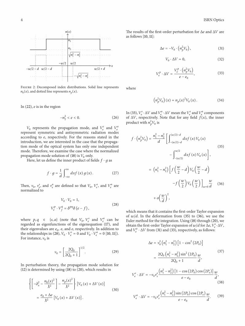


![Using Trees To Compute Approximate Solutions to Ordinary ...papers.rgrossman.com/proc-013.pdf · used in perturbation theory by Rand [59] and Meyer [54], in celestial mechanics by](https://img.pdfslide.net/doc/110x75/5f03991c7e708231d409d78b/using-trees-to-compute-approximate-solutions-to-ordinary-used-in-perturbation.jpg)