Research Article Preliminary Experimental Study on

Research ArticlePreliminary Experimental Study on Pressure Loss Coefficients ofExhaust Manifold Junction

Xiao-lu Lu,1 Kun Zhang,1 Wen-hui Wang,1 Shao-ming Wang,2 and Kang-yao Deng1

1 Education Ministry Key Laboratory for Power Machinery and Engineering, Shanghai Jiaotong University, Shanghai 200240, China2 Technology Center of the SAIC Motor, Shanghai 201800, China

Correspondence should be addressed to Kang-yao Deng; [email protected]

Received 29 August 2013; Revised 6 January 2014; Accepted 24 January 2014; Published 13 March 2014

Academic Editor: Masaru Ishizuka

Copyright © 2014 Xiao-lu Lu et al. This is an open access article distributed under the Creative Commons Attribution License,which permits unrestricted use, distribution, and reproduction in any medium, provided the original work is properly cited.

The flow characteristic of exhaust system has an important impact on inlet boundary of the turbine. In this paper, high speed flowin a diesel exhaust manifold junction was tested and simulated. The pressure loss coefficient of the junction flow was analyzed. Thesteady experimental results indicated that both of static pressure loss coefficients 𝐿

13and 𝐿

23first increased and then decreased

with the increase of mass flow ratio of lateral branch and public manifold. The total pressure loss coefficient 𝐾13always increased

with the increase of mass flow ratio of junctions 1 and 3. The total pressure loss coefficient 𝐾23first increased and then decreased

with the increase of mass flow ratio of junctions 2 and 3.These pressure loss coefficients of the exhaust pipe junctions can be used inexhaust flow and turbine inlet boundary conditions analysis. In addition, simulating calculation was conducted to analyze the effectof branch angle on total pressure loss coefficient. According to the calculation results, total pressure loss coefficient was almost thesame at lowmass flow rate of branch manifold 1 but increased with lateral branch angle at high mass flow rate of branch manifold 1.

1. Introduction

A very substantial part of the design of a turbochargingsystem is the exhaust pipe construction. This is because theflow characteristic of the exhaust system has an importantimpact on the inlet boundary of the turbine, which affects thepower out of the turbine. The principle means to understandthat the flow characteristics are the numerical simulation. Byusing a numerical simulation, it is possible to understandthe exhaust pipe pressure wave forms and their propagationcharacteristics and analyze the use of the exhaust energy andcylinder scavenging as well as design and optimization of theexhaust system. In an exhaust system, the pipe is generallya one-dimensional pipe, so a one-dimensional flow analysiscan be used. However, there are three-dimensional flows inthe exhaust manifold junction of the exhaust pipe system;so, using a one-dimensional numerical simulation will resultin a large error. Accuracy in the pressure loss coefficientsimulation of the exhaust manifold junction of the exhaustpipe system is essential. During the existing one-dimensional

simulation of the engine, when the exhaust gas passes with ahigher flow rate, the accuracy of the calculated pressure lossof the tee is relatively low.

In papers [1–6], several researchers have studied thepressure loss coefficient of the exhaustmanifold junction.Theresearch showed that the pressure loss coefficient is mainlyaffected by the flow ratio between the public manifold andbranch manifold and that 12 circulation types of the pressureloss coefficient calculation formula are deductible. However,during the theoretical derivation process, the junction fluidis assumed to be an incompressible fluid. When the publicmanifold Mach number is greater than 0.2, the pressure losscoefficients between the calculated and experimental werequite different. In papers [7–9], some experimental researchon the pressure lossmodel of the exhaustmanifold junction ofthe “T” type was done.The research showed that the pressureloss coefficient was related not only to the flow ratio betweenthe public manifold and branch manifold but also to theMach number in the public manifold. However, during theexperiment, the diameter of the branch manifold was only

Hindawi Publishing CorporationInternational Journal of Rotating MachineryVolume 2014, Article ID 316498, 10 pageshttp://dx.doi.org/10.1155/2014/316498

2 International Journal of Rotating Machinery

Temperature sensor 1

Pressure sensor 1

Differential pressure sensor 1

Temperature sensor 2

Differential pressure sensor 2

Back pressure valve Branch manifold 3 Branch manifold 2

Temperaturesensor 2

Branch manifold 1

Differential pressure sensor 3Temperature

sensor 4

Pitot tubePressuresensor 3

Bleed valve

Step motorCompressorPublic manifold

Flow controlvalve 1

Flow controlvalve 2

Mass flow sensor

Figure 1: Schematic diagram of the experiment.

Flow control valve

Pipeline

Lift of flow control valve

Figure 2: Schematic diagram of the valve.

12mm, which was much smaller than that in a real engine,and the flow type of the junction was not common in exhaustmanifold.

In this paper, the high speed flow in a diesel exhaust man-ifold junction was measured. The pressure loss coefficientsof the exhaust manifold junction with high speed flow wereanalyzed. The results provide reference for the pressure lossjunction model considering gas compressibility. At last, theinternal flow phenomena of junction were analyzed by CFDmodel, and the effect of branch angle on total pressure losscoefficient was also studied.

2. Materials and Experiment

A schematic diagram of the experiment is shown in Figure 1.A 400 kW step motor was used to drive the compressor,and the bleed valve was installed behind the compressorto prevent the compressor from surging during the test.

Measuring point 1

Point A

Measuring point 3 Measuring point 2

Figure 3: Photograph of the junction.

The pressure sensor 2, Pitot tube, and temperature sensor 4were installed in the public manifold that comes after thecompressor. Pressure sensor 3 was installed behind the Pitottube to measure the difference between the total pressureand static pressure. Flow control valves 1 and 2 were the gatevalves, and schematic diagram is shown in Figure 2.The flowwithin the pipe was changed by lifting the valve. A mass flowsensor that could measure range ratio of 1000 : 1 was installedafter flow control valve 2 to measure the mass flow of the gasin branch manifold 2. Temperature sensors were installed inthe manifold branches 1 to 3 to measure the gas temperature.Pressure sensor 2 was installed in the branch manifold tomeasure the pressure. Differential pressure transducer 1 wasinstalled to measure the pressure difference between branchmanifold 1 and branch manifold 3. Differential pressuretransducer 2 was installed to measure the pressure differencebetween branch manifold 2 and branch manifold 3. Toregulate the back pressure in branch manifold 3, a backpressure valve was installed after branch manifold 3.

A photograph of the junction is shown in Figure 3. Thejunctionwasmade by stainless steel to reduce thewall frictionloss. The diameter of the three branch manifolds was 66mm,which is equal to the diameter of the pulse turbochargingsystem of a heavy duty vehicular diesel engine. The anglebetween branch manifold 1 and 2 was 45∘. The point Awas the intersection point of the center lines. The distancesbetween point A and measuring point 1, between point Aand measuring point 2, and between point A and measuringpoint 3 were 260mm, which was equal to 4 times of the pipediameter. The lengths of branch manifold 1, branch manifold2, and branch manifold 3 were all 0.65m.

International Journal of Rotating Machinery 3

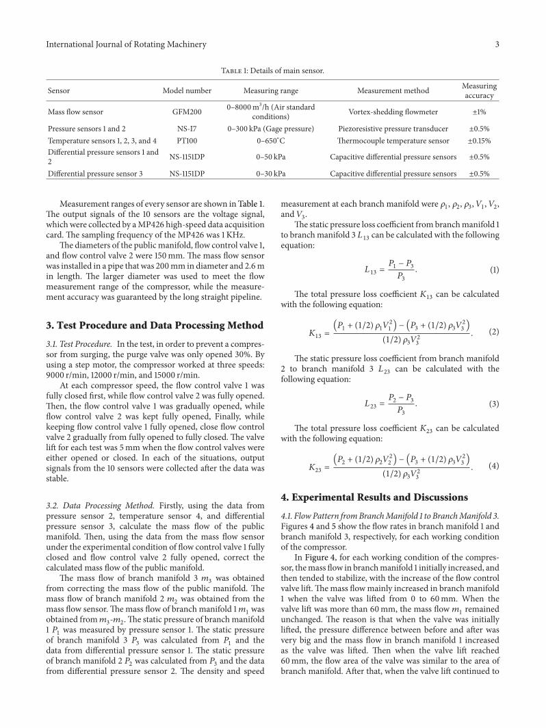
Table 1: Details of main sensor.

Sensor Model number Measuring range Measurement method Measuringaccuracy

Mass flow sensor GFM200 0–8000m3/h (Air standardconditions) Vortex-shedding flowmeter ±1%

Pressure sensors 1 and 2 NS-I7 0–300 kPa (Gage pressure) Piezoresistive pressure transducer ±0.5%Temperature sensors 1, 2, 3, and 4 PT100 0–650∘C Thermocouple temperature sensor ±0.15%Differential pressure sensors 1 and2 NS-1151DP 0–50 kPa Capacitive differential pressure sensors ±0.5%

Differential pressure sensor 3 NS-1151DP 0–30 kPa Capacitive differential pressure sensors ±0.5%

Measurement ranges of every sensor are shown in Table 1.The output signals of the 10 sensors are the voltage signal,whichwere collected by aMP426 high-speed data acquisitioncard. The sampling frequency of the MP426 was 1 KHz.

The diameters of the publicmanifold, flow control valve 1,and flow control valve 2 were 150mm. The mass flow sensorwas installed in a pipe that was 200mm in diameter and 2.6min length. The larger diameter was used to meet the flowmeasurement range of the compressor, while the measure-ment accuracy was guaranteed by the long straight pipeline.

3. Test Procedure and Data Processing Method

3.1. Test Procedure. In the test, in order to prevent a compres-sor from surging, the purge valve was only opened 30%. Byusing a step motor, the compressor worked at three speeds:9000 r/min, 12000 r/min, and 15000 r/min.

At each compressor speed, the flow control valve 1 wasfully closed first, while flow control valve 2 was fully opened.Then, the flow control valve 1 was gradually opened, whileflow control valve 2 was kept fully opened, Finally, whilekeeping flow control valve 1 fully opened, close flow controlvalve 2 gradually from fully opened to fully closed. The valvelift for each test was 5mm when the flow control valves wereeither opened or closed. In each of the situations, outputsignals from the 10 sensors were collected after the data wasstable.

3.2. Data Processing Method. Firstly, using the data frompressure sensor 2, temperature sensor 4, and differentialpressure sensor 3, calculate the mass flow of the publicmanifold. Then, using the data from the mass flow sensorunder the experimental condition of flow control valve 1 fullyclosed and flow control valve 2 fully opened, correct thecalculated mass flow of the public manifold.

The mass flow of branch manifold 3 𝑚3was obtained

from correcting the mass flow of the public manifold. Themass flow of branch manifold 2 𝑚

2was obtained from the

mass flow sensor.Themass flow of branch manifold 1𝑚1was

obtained from𝑚3-𝑚2.The static pressure of branchmanifold

1 𝑃1was measured by pressure sensor 1. The static pressure

of branch manifold 3 𝑃3was calculated from 𝑃

1and the

data from differential pressure sensor 1. The static pressureof branch manifold 2 𝑃

2was calculated from 𝑃

3and the data

from differential pressure sensor 2. The density and speed

measurement at each branch manifold were 𝜌1, 𝜌2, 𝜌3, 𝑉1, 𝑉2,

and 𝑉3.

The static pressure loss coefficient frombranchmanifold 1to branchmanifold 3 𝐿

13can be calculated with the following

equation:

𝐿13=𝑃1− 𝑃3

𝑃3

. (1)

The total pressure loss coefficient 𝐾13

can be calculatedwith the following equation:

𝐾13=

(𝑃1+ (1/2) 𝜌

1𝑉2

1) − (𝑃

3+ (1/2) 𝜌

3𝑉2

3)

(1/2) 𝜌3𝑉2

3

. (2)

The static pressure loss coefficient from branch manifold2 to branch manifold 3 𝐿

23can be calculated with the

following equation:

𝐿23=𝑃2− 𝑃3

𝑃3

. (3)

The total pressure loss coefficient 𝐾23

can be calculatedwith the following equation:

𝐾23=

(𝑃2+ (1/2) 𝜌

2𝑉2

2) − (𝑃

3+ (1/2) 𝜌

3𝑉2

3)

(1/2) 𝜌3𝑉2

3

. (4)

4. Experimental Results and Discussions

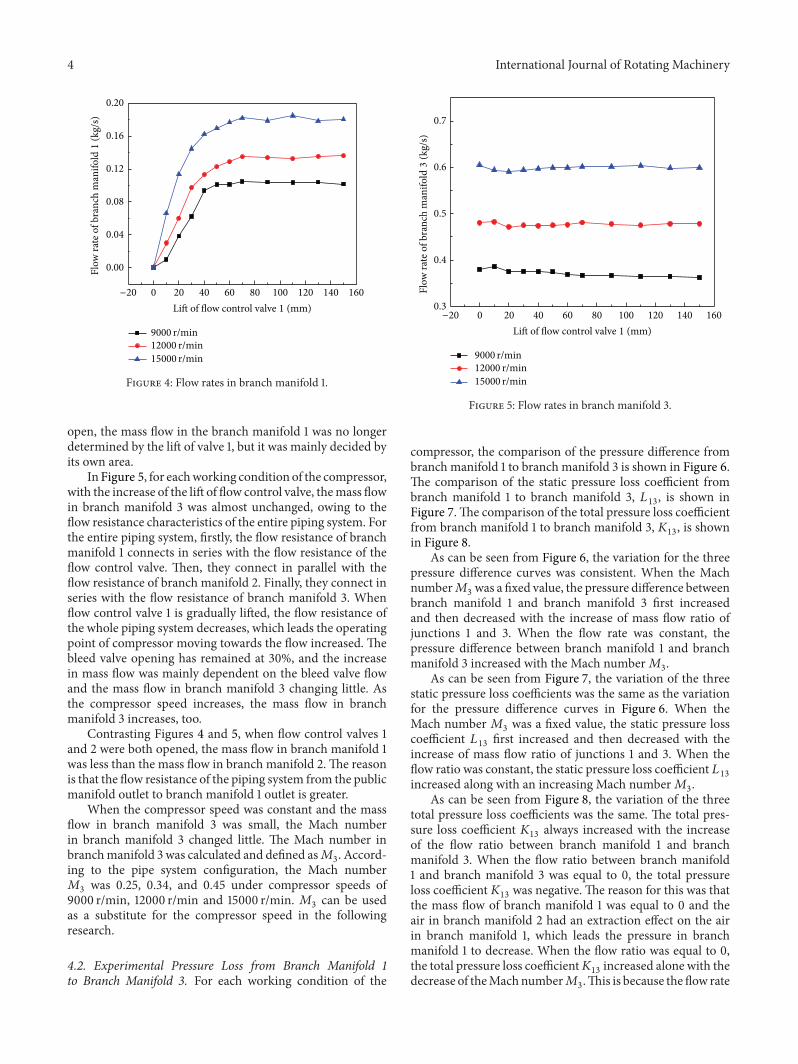
4.1. FlowPattern fromBranchManifold 1 to BranchManifold 3.Figures 4 and 5 show the flow rates in branch manifold 1 andbranch manifold 3, respectively, for each working conditionof the compressor.

In Figure 4, for each working condition of the compres-sor, themass flow in branchmanifold 1 initially increased, andthen tended to stabilize, with the increase of the flow controlvalve lift.Themass flowmainly increased in branchmanifold1 when the valve was lifted from 0 to 60mm. When thevalve lift was more than 60mm, the mass flow 𝑚

1remained

unchanged. The reason is that when the valve was initiallylifted, the pressure difference between before and after wasvery big and the mass flow in branch manifold 1 increasedas the valve was lifted. Then when the valve lift reached60mm, the flow area of the valve was similar to the area ofbranch manifold. After that, when the valve lift continued to


0 20 40 60 80 100 120 140 160

0.00

0.04

0.08

0.12

0.16

0.20

−20Lift of flow control valve 1 (mm)

Flow

rate

of b

ranc

h m

anifo

ld1

(kg/

s)

9000 r/min12000 r/min15000 r/min

Figure 4: Flow rates in branch manifold 1.

open, the mass flow in the branch manifold 1 was no longerdetermined by the lift of valve 1, but it was mainly decided byits own area.

In Figure 5, for eachworking condition of the compressor,with the increase of the lift of flow control valve, themass flowin branch manifold 3 was almost unchanged, owing to theflow resistance characteristics of the entire piping system. Forthe entire piping system, firstly, the flow resistance of branchmanifold 1 connects in series with the flow resistance of theflow control valve. Then, they connect in parallel with theflow resistance of branch manifold 2. Finally, they connect inseries with the flow resistance of branch manifold 3. Whenflow control valve 1 is gradually lifted, the flow resistance ofthe whole piping system decreases, which leads the operatingpoint of compressor moving towards the flow increased. Thebleed valve opening has remained at 30%, and the increasein mass flow was mainly dependent on the bleed valve flowand the mass flow in branch manifold 3 changing little. Asthe compressor speed increases, the mass flow in branchmanifold 3 increases, too.

Contrasting Figures 4 and 5, when flow control valves 1and 2 were both opened, the mass flow in branch manifold 1was less than the mass flow in branch manifold 2. The reasonis that the flow resistance of the piping system from the publicmanifold outlet to branch manifold 1 outlet is greater.

When the compressor speed was constant and the massflow in branch manifold 3 was small, the Mach numberin branch manifold 3 changed little. The Mach number inbranchmanifold 3 was calculated and defined as𝑀

3. Accord-

ing to the pipe system configuration, the Mach number𝑀3was 0.25, 0.34, and 0.45 under compressor speeds of

9000 r/min, 12000 r/min and 15000 r/min. 𝑀3can be used

as a substitute for the compressor speed in the followingresearch.

4.2. Experimental Pressure Loss from Branch Manifold 1to Branch Manifold 3. For each working condition of the

0 20 40 60 80 100 120 140 1600.3

0.4

0.5

0.6

0.7

−20

9000 r/min12000 r/min15000 r/min

Lift of flow control valve 1 (mm)

Flow

rate

of b

ranc

h m

anifo

ld3

(kg/

s)Figure 5: Flow rates in branch manifold 3.

compressor, the comparison of the pressure difference frombranch manifold 1 to branch manifold 3 is shown in Figure 6.The comparison of the static pressure loss coefficient frombranch manifold 1 to branch manifold 3, 𝐿

13, is shown in

Figure 7.The comparison of the total pressure loss coefficientfrom branch manifold 1 to branch manifold 3, 𝐾

13, is shown

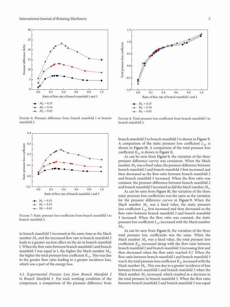
in Figure 8.As can be seen from Figure 6, the variation for the three

pressure difference curves was consistent. When the Machnumber𝑀

3was a fixed value, the pressure difference between

branch manifold 1 and branch manifold 3 first increasedand then decreased with the increase of mass flow ratio ofjunctions 1 and 3. When the flow rate was constant, thepressure difference between branch manifold 1 and branchmanifold 3 increased with the Mach number𝑀

3.

As can be seen from Figure 7, the variation of the threestatic pressure loss coefficients was the same as the variationfor the pressure difference curves in Figure 6. When theMach number𝑀

3was a fixed value, the static pressure loss

coefficient 𝐿13

first increased and then decreased with theincrease of mass flow ratio of junctions 1 and 3. When theflow ratio was constant, the static pressure loss coefficient 𝐿

13

increased along with an increasing Mach number𝑀3.

As can be seen from Figure 8, the variation of the threetotal pressure loss coefficients was the same. The total pres-sure loss coefficient 𝐾

13always increased with the increase

of the flow ratio between branch manifold 1 and branchmanifold 3. When the flow ratio between branch manifold1 and branch manifold 3 was equal to 0, the total pressureloss coefficient𝐾

13was negative. The reason for this was that

the mass flow of branch manifold 1 was equal to 0 and theair in branch manifold 2 had an extraction effect on the airin branch manifold 1, which leads the pressure in branchmanifold 1 to decrease. When the flow ratio was equal to 0,the total pressure loss coefficient𝐾

13increased alone with the

decrease of theMachnumber𝑀3.This is because the flow rate


0.0 0.2 0.4 0.6 0.8 1.00

5

10

15

20

25

30

Pres

sure

diff

eren

ce (k

Pa)

Ratio of flow rate of branch manifold 1 and 3

M3 = 0.25

M3 = 0.34

M3 = 0.45

Figure 6: Pressure difference from branch manifold 1 to branchmanifold 3.

0.0 0.2 0.4 0.6 0.8 1.0

0.0

0.1

0.2

0.3

0.4


Stat

ic p

ress

ure l

oss c

oeffi

cien

t

M3 = 0.25

M3 = 0.34

M3 = 0.45

−0.1

Figure 7: Static pressure loss coefficient from branch manifold 1 tobranch manifold 3.

in branch manifold 3 increased at the same time as the Machnumber𝑀

3and the increased flow rate in branch manifold 3

leads to a greater suction effect on the air in branch manifold1.When the flow ratio between branchmanifold 1 and branchmanifold 3 was equal to 1, the higher the Mach number𝑀

3,

the higher the total pressure loss coefficient𝐾13.This was due

to the greater flow ratio leading to a greater incidence loss,which was a part of the energy loss.

4.3. Experimental Pressure Loss from Branch Manifold 2to Branch Manifold 3. For each working condition of thecompressor, a comparison of the pressure difference from

0.0 0.2 0.4 0.6 0.8 1.0

0.0

0.5

1.0

1.5


Tota

l pre

ssur

e los

s coe

ffici

ent

−1.0

−0.5

M3 = 0.25

M3 = 0.34

M3 = 0.45

Figure 8: Total pressure loss coefficient from branch manifold 1 tobranch manifold 3.

branchmanifold 2 to branchmanifold 3 is shown in Figure 9.A comparison of the static pressure loss coefficient 𝐿

23is

shown in Figure 10. A comparison of the total pressure losscoefficient 𝐾

23is shown in Figure 11.

As can be seen from Figure 9, the variation of the threepressure difference curves was consistent. When the Machnumber𝑀

3was a fixed value, the pressure difference between

branch manifold 2 and branch manifold 3 first increased andthen decreased as the flow ratio between branch manifold 2and branch manifold 3 increased. When the flow ratio wasconstant, the pressure difference between branch manifold 2and branchmanifold 3 increased as did theMachnumber𝑀

3.

As can be seen from Figure 10, the variation of the threestatic pressure loss coefficients was the same as the variationfor the pressure difference curves in Figure 9. When theMach number 𝑀

3was a fixed value, the static pressure

loss coefficient 𝐿23

first increased and then decreased as theflow ratio between branch manifold 2 and branch manifold3 increased. When the flow ratio was constant, the staticpressure loss coefficient 𝐿

23increased with theMach number

𝑀3.As can be seen from Figure 11, the variation of the three

total pressure loss coefficients was the same. When theMach number 𝑀

3was a fixed value, the total pressure loss

coefficient 𝐾23

increased along with the flow ratio betweenbranchmanifold 2 and branchmanifold 3 increasing first andthen decreased when the flow ratio reached 0.7. When theflow ratio between branch manifold 1 and branch manifold 3was 0, the total pressure loss coefficient𝐾

23increasedwith the

Mach number𝑀3. This was due to a greater incidence of loss

between branch manifold 1 and branch manifold 3 when theMach number𝑀

3increased, which resulted in a decrease in

the total pressure in branch manifold 3. When the flow ratiobetween branch manifold 2 and branch manifold 3 was equal


0.0 0.2 0.4 0.6 0.8 1.00

5

10

15

20

25

30


Pres

sure

diff

eren

ce (k

Pa)

M3 = 0.25

M3 = 0.34

M3 = 0.45

Figure 9: Pressure difference from branch manifold 2 to branchmanifold 3.

0.0 0.2 0.4 0.6 0.8 1.0

0.00

0.05

0.10

0.15

0.20

0.25

0.30

0.35

Stat

ic p

ress

ure l

oss c

oeffi

cien

t


−0.05

M3 = 0.25

M3 = 0.34

M3 = 0.45

Figure 10: Static pressure loss coefficient from branchmanifold 2 tobranch manifold 3.

to 1, the total pressure loss coefficient 𝐾23increased with the

Mach number𝑀3. That was because there was no air flow in

branchmanifold 1, and the flow rate between branchmanifold2 and branchmanifold 3 was the same.The total pressure losscoefficient𝐾

23mainly depended on the local pressure loss in

branch manifold 1 and its effect on branch manifold 2.Contrast Figure 10 with Figure 11, and it can be deter-

mined that the maximum value of the static pressure losscoefficient 𝐿

23and the total pressure loss coefficient 𝐾

23are

obtained at the same flow ratio 0.7.This was due to the impactloss of flow between branch manifold 1 and branch manifold

0.0 0.2 0.4 0.6 0.8 1.0

0.0

0.2

0.4

0.6

0.8

1.0

1.2

Tota

l pre

ssur

e los

s coe

ffici

ent


M3 = 0.25

M3 = 0.34

M3 = 0.45

Figure 11: Total pressure loss coefficient from branch manifold 2 tobranch manifold 3.

2 having the largest effect on the air’s energy loss in branchmanifold 2 at that moment.

Contrast Figure 7 with Figure 10, and it can be deter-mined that the maximum value of the static pressure losscoefficient 𝐿

13appeared when the flow ratio between branch

manifold 1 and branch manifold 3 was equal to 0.3. Inaddition, the maximum value of the static pressure losscoefficient 𝐿

23appeared when the flow ratio between branch

manifold 2 and branch manifold 3 was equal to 0.7. Themaximum values of 𝐿

13and 𝐿

23as well as 𝐾

23, the total

pressure loss coefficient, all appeared at the same condition.Contrast Figure 8with Figure 11, and it can be determined

that when the flow ratio was unchanged, the total pressureloss coefficient 𝐾

23was strongly influenced by the Mach

number𝑀3.

5. Junction Simulation and Discussions

5.1. 45∘ Junction Simulation. As the flow phenomena inthe manifold could not be reflect by experiment, the flowfield of junction was simulated by AVL-Fire. The size ofsimulationmodel was the same as themeasuredmodel whichis showed in Figure 12. The inlet boundary conditions ofbranch manifolds 1 and 2 were mass flow, and the outletboundary condition of branch manifold 3 was atmosphericpressure. The Mach numbers in branch manifold 3𝑀

3were

0.25, 0.34, and 0.45. For each working condition, the flowratio between branch manifold 1 and branch manifold 3 𝑄

13

changed from 0 to 1.The comparison of total pressure loss coefficient between

calculated and measured values was showed in Figure 13.The values calculated by CFD were in good agreement withexperimental observations. When the flow ratio betweenbranch manifold 1 and branch manifold 3𝑄

13was equal to 0,

the junction could be seen as straight pipe. Since the influence


Inlet boundary: mass flowof branch manifold 1

Outlet boundary:atmospheric pressure

Inlet boundary: mass flowof branch manifold 2

Figure 12: Simulation model of junction.

0.0 0.2 0.4 0.6 0.8 1.0

0.0

0.5

1.0

1.5

2.0

Ratio of flow rate of branch manifolds 1 and 3

−2.0

−1.5

−1.0

−0.5

Tota

l pre

ssur

e los

s coe

ffici

entK

13

Measured M3 = 0.25

Measured M3 = 0.34

Measured M3 = 0.45

Calculated M3 = 0.25



(a) 𝐾13

0.0 0.2 0.4 0.6 0.8 1.0

0.0

0.5

1.0

1.5


−2.0

−1.5

−1.0

−0.5

Measured M3 = 0.25

Measured M3 = 0.34

Measured M3 = 0.45




Tota

l pre

ssur

e los

s coe

ffici

entK

23

(b) 𝐾23

Figure 13: Comparison of total pressure loss coefficient between calculated and measured values.

of branch manifold 1 can be ignored, the calculated valuesalmost equal to measured values. With the increase of flowrate in branch manifold 1, simulation data were slightly lessthan the test data, but the change trend of the calculatedvalues were the same as the measured values. Simulationresults could reflect the change trend of total pressure losscoefficients 𝐾

13and 𝐾

23. As can be seen from Figure 13, the

calculated value of total pressure loss coefficient 𝐾13

alwaysincreased when the flow ratio between branch manifold 1and branch manifold 3 increased, which is the same as themeasured value. The calculated value of total pressure losscoefficient 𝐾

23first increased and then decreased when the

flow ratio between branch manifold 2 and branch manifold 3reached 0.7.

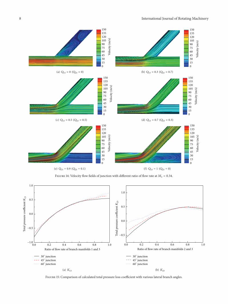
By using CFD analysis software, the internal flow phe-nomenon of junction could be analyzed. Figure 14 showsthe velocity fields of junction flow with different mass flowratio at 𝑀

3= 0.34. The mass flow ratio between branch

manifold 1 and branch manifold 3 𝑄13

changed from 0 to 1at the same time when the mass flow ratio between branchmanifold 2 and branch manifold 3 𝑄

23changed from 1 to 0.

The uniformity of flow at branch joint is increased with theincrease of the flow in branchmanifold 1.When themass flow

ratio 𝑄13

reached 0.6, vortex appeared in the junction andbecomes stronger with the increase of𝑄

13. Meanwhile, as can

be seen from velocity fields of the junction, the flow impactfrom branch manifold 1 to branch manifold 2 was enhancedwith the increase of 𝑄

13. Because of the above reasons, the

total pressure loss coefficient 𝐾13

always increased with theincrease of 𝑄

13. When the mass flow ratio 𝑄

23was equal to

1, the total pressure loss coefficient 𝐾23mainly depended on

the local pressure loss in branch manifold 1 and its effect onbranch manifold 2. Since the total pressure value of branchmanifold 2 decreased with the reduction of flow rate, thetotal pressure loss coefficient 𝐾

23decreased alone with the

decrease of the flow ratio 𝑄23.

The comparison of simulation and test results showed thatthe following.

(1) Simulation could reflect the change trend of totalpressure loss coefficient, but it could not predict itsvalue accurately.

(2) It is necessary to carry out the experimental studyto obtain the accurate value of the total pressure losscoefficient.


Velo

city

(m/s

)

150

135

120

105

90

75

60

45

30

15

0

(a) 𝑄13 = 0 (𝑄23 = 0)

Velo

city

(m/s

)

150

135

120

105

90

75

60

45

30

15

0

(b) 𝑄13 = 0.3 (𝑄23 = 0.7)

150

135

120

105

90

75

60

45

30

15

0

Velo

city

(m/s

)

(c) 𝑄13 = 0.5 (𝑄23 = 0.5)

150

135

120

105

90

75

60

45

30

15

0

Velo

city

(m/s

)

(d) 𝑄13 = 0.7 (𝑄23 = 0.3)

150

135

120

105

90

75

60

45

30

15

0

Velo

city

(m/s

)

(e) 𝑄13 = 0.9 (𝑄23 = 0.1)

150

135

120

105

90

75

60

45

30

15

0

Velo

city

(m/s

)

(f) 𝑄13 = 1 (𝑄23 = 0)

Figure 14: Velocity flow fields of junction with different ratio of flow rate at𝑀3= 0.34.

0.0 0.2 0.4 0.6 0.8 1.0

0.0

0.5

1.0


−0.5

−1.0

30∘ junction

45∘ junction

60∘ junction

Tota

l pre

ssur

e coe

ffici

entK

13

(a) 𝐾13

0.0 0.2 0.4 0.6 0.8 1.0

0.0

0.5

1.0


−0.5Tota

l pre

ssur

e coe

ffici

entK

23

30∘ junction

45∘ junction

60∘ junction

(b) 𝐾23

Figure 15: Comparison of calculated total pressure loss coefficient with various lateral branch angles.


150

135

120

105

90

75

60

45

30

15

0

Velo

city

(m/s

)

(a) 30∘ junction

150

135

120

105

90

75

60

45

30

15

0

Velo

city

(m/s

)

(b) 45∘ junction

150

135

120

105

90

75

60

45

30

15

0

Velo

city

(m/s

)

(c) 60∘ junction

Figure 16: Velocity flow fields of junction with different lateral branch angles at 𝑄13= 0.9, and𝑀

3= 0.34.

5.2. 30∘ and 60∘ Junction Simulation. As 45∘ junction is acommon type in the exhaust system, the test was based onthis type of manifold. But the angle between the branchmanifold 1 and the branch manifold 2 may affects the flowcondition in themanifold, and other structures also should bestudied. As simulation results could reflect the change trendof total pressure loss coefficient, CFD analysis software wasused to analyze the effect of branch angle on total pressure losscoefficient. Based on the previous studies, simulation modelsof 30∘ and 60∘ junction were set up.The boundary conditionsof the models were the same as 45∘ junction, and the Machnumber in branch manifold 3𝑀

3was 0.34. Figure 15 shows

the comparison of calculated total pressure loss coefficientwith various lateral branch angles. As can be seen from thefigures, when the branchmanifold 1 was at lowmass flow rate(the branch manifold 1 has less effect on branch manifolds 2and 3), total pressure loss coefficients of different angles werealmost the same.With the increase ofmass flow rate of branchmanifold 1 and the reduction of mass flow rate of branchmanifold 2, the differences between different structures of themanifold are obvious. When the branch manifold 1 was athigh mass flow rate, the greater the lateral branch angle, thegreater the total pressure loss coefficients𝐾

13and𝐾

23.

Velocity fields of junction flow with different lateralbranch angles at 𝑄

13= 0.9 and 𝑀

3= 0.34 are shown in

Figure 16. The uniformity of flow at branch joint is increasedwith the increase of lateral branch angle, and the flow impactbetween branch manifolds 1 and 2 increased significantly.Meanwhile, vortex appeared in the junction, and it becomesstronger with the increase of the lateral branch angle. For theabove reasons, the total pressure loss coefficient𝐾

13increased

alone with the increase of lateral branch angle.

6. Conclusions

The high speed flow in a diesel exhaust manifold 45∘ junctionwas tested, and three junctions with different lateral branch

angles were simulated by CFD analysis software. The steadyexperimental and simulated results indicated that the follow-ing.

(1) The static pressure loss coefficient 𝐿13first increased

and then decreased along with the flow ratio betweenbranch manifold 1 and branch manifold 3 increasing;the variation law of the static pressure loss coefficient𝐿23was similar to 𝐿

13.

(2) The total pressure loss coefficient 𝐾13

alwaysincreased with the increase of the flow ratio betweenbranch manifold 1 and branch manifold 3; the totalpressure loss coefficient 𝐾

23first increased and then

decreased with the increase of the flow ratio betweenbranch manifold 2 and branch manifold 3.

(3) The maximum values for the static pressure losscoefficient 𝐿

13, the static pressure loss coefficient 𝐿

23,

and the total pressure loss coefficient𝐾13appeared at

exactly the same condition.

(4) When the flow ratiowas unchanged, the total pressureloss coefficient 𝐾

23was strongly influenced by the

Mach number𝑀3.

(5) Simulation results predicted the change trend of totalpressure loss coefficient, but they could not predicttheir value accurately. It is necessary to carry out theexperimental study to obtain the accurate value of thetotal pressure loss coefficient.

(6) When the branch manifold 1 was at low mass flowrate, total pressure loss coefficients of different branchangles were almost the same. At high mass flow rate,the total pressure loss coefficients increased alonewith the increase of lateral branch angle.


Conflict of Interests

The authors declare that there is no conflict of interestsregarding the publication of this paper.

References

[1] D. E. Winterbone and R. J. Pearson, Design Techniques forEngine Manifolds—Wave Action Methods for IC Engines, Pro-fessional Engineering Publications, London, UK, 1999.

[2] D. E. Winterbone and R. J. Pearson, Theory of Engine ManifoldDesign—Wave Action Methods for IC Engines, ProfessionalEngineering Publications, London, UK, 2000.

[3] M. D. Bassett, R. J. Pearson, N. P. Fleming et al., “A Multi-PipeJunction Model for One Dimensional Gas-Dynamic Simula-tions,” SAE Paper 2003-01-0370, 2003.

[4] M. D. Bassett, D. E.Winterbone, and R. J. Pearson, “Calculationof steady flow pressure loss coefficients for pipe junctions,”Proceedings of the Institution ofMechanical Engineers C, vol. 215,no. 8, pp. 861–882, 2001.

[5] M. D. Bassett, N. P. Fleming, and R. J. Pearson, “Modellingengines with pulse converted exhaust manifolds using one-dimensional techniques,” SAE Paper 2000-01-0290, 2000.

[6] R. J. Pearson, R. J. Pearson, andD. E.Winterbone, “Estimationofsteady flow loss coefficients forpulse converter junctions inexhaust manifolds,” in Proceedings of the 6th InternationalConference on Turbocharging and Air Management Systems, IMech E Paper No. C554/022/98, I Mech E HQ, London, UK,November1998.

[7] J. Perez-Garcıa, E. Sanmiguel-Rojas, J. Hernandez-Grau, andA. Viedma, “Numerical and experimental investigations oninternal compressible flow at T-type junctions,” ExperimentalThermal and Fluid Science, vol. 31, no. 1, pp. 61–74, 2006.

[8] J. Perez-Garcıa, E. Sanmiguel-Rojas, and A. Viedma, “Newcoefficient to characterize energy losses in compressible flowat T-junctions,” Applied Mathematical Modelling, vol. 34, no. 12,pp. 4289–4305, 2010.

[9] J. Perez-Garcıa, E. Sanmiguel-Rojas, and A. Viedma, “Newexperimental correlations to characterize compressible flowlosses at 90-degree T-junctions,” Experimental Thermal andFluid Science, vol. 33, no. 2, pp. 261–266, 2009.

International Journal of

AerospaceEngineeringHindawi Publishing Corporationhttp://www.hindawi.com Volume 2014

RoboticsJournal of

Hindawi Publishing Corporationhttp://www.hindawi.com Volume 2014


Active and Passive Electronic Components

Control Scienceand Engineering

Journal of



RotatingMachinery


Hindawi Publishing Corporation http://www.hindawi.com

Journal ofEngineeringVolume 2014

Submit your manuscripts athttp://www.hindawi.com

VLSI Design



Shock and Vibration


Civil EngineeringAdvances in

Acoustics and VibrationAdvances in



Electrical and Computer Engineering

Journal of

Advances inOptoElectronics

Hindawi Publishing Corporation http://www.hindawi.com

Volume 2014

The Scientific World JournalHindawi Publishing Corporation http://www.hindawi.com Volume 2014

SensorsJournal of


Modelling & Simulation in EngineeringHindawi Publishing Corporation http://www.hindawi.com Volume 2014


Chemical EngineeringInternational Journal of Antennas and

Propagation




Navigation and Observation



DistributedSensor Networks


Documents

Research Article Preliminary Experimental Study on