Research Article Publication Bias in Meta-Analysis

Research ArticlePublication Bias in Meta-Analysis Confidence Intervals forRosenthalrsquos Fail-Safe Number

Konstantinos C Fragkos12 Michail Tsagris3 and Christos C Frangos4

1 Department of Economics Mathematics and Statistics Birkbeck University of London Malet Street London WC1E 7HX UK2Division of Medicine University College London Rockefeller Building 21 University Street London WC1E 6JJ UK3 College of Engineering and Technology American University of the Middle East Egaila Kuwait4Department of Business Administration Technological Educational Institute (TEI) of Athens 122 43 Athens Greece

Correspondence should be addressed to Konstantinos C Fragkos constantinosfrangos09uclacuk

Received 23 June 2014 Revised 5 October 2014 Accepted 20 October 2014 Published 3 December 2014

Academic Editor Giuseppe Biondi-Zoccai

Copyright copy 2014 Konstantinos C Fragkos et alThis is an open access article distributed under theCreative CommonsAttributionLicense which permits unrestricted use distribution and reproduction in anymedium provided the originalwork is properly cited

The purpose of the present paper is to assess the efficacy of confidence intervals for Rosenthalrsquos fail-safe number AlthoughRosenthalrsquos estimator is highly used by researchers its statistical properties are largely unexplored First of all we developedstatistical theorywhich allowedus to produce confidence intervals for Rosenthalrsquos fail-safe numberThiswas produced by discerningwhether the number of studies analysed in a meta-analysis is fixed or random Each case produces different variance estimatorsFor a given number of studies and a given distribution we provided five variance estimators Confidence intervals are examinedwith a normal approximation and a nonparametric bootstrap The accuracy of the different confidence interval estimates was thentested by methods of simulation under different distributional assumptions The half normal distribution variance estimator hasthe best probability coverage Finally we provide a table of lower confidence intervals for Rosenthalrsquos estimator

1 Introduction

Meta-analysis refers to methods focused on contrasting andcombining results from different studies in the hope of iden-tifying patterns among study results sources of disagreementamong those results or other interesting relationships thatmay come to light in the context of multiple studies [1] Inits simplest form this is normally done by identification of acommon measure of effect size of which a weighted averagemight be the output of a meta-analysis The weighting mightbe related to sample sizes within the individual studies [2 3]More generally there are other differences between the studiesthat need to be allowed for but the general aim of a meta-analysis is to more powerfully estimate the true effect sizeas opposed to a less precise effect size derived in a singlestudy under a given single set of assumptions and conditions[4] For reviews on meta-analysis models see [2 5 6] Meta-analysis can be applied to various effect sizes collected fromindividual studies These include odds ratios and relativerisks standardized mean difference Cohenrsquos 119889 Hedgesrsquo 119892and Glassrsquos Δ correlation coefficient and relative metrics

sensitivity and specificity from diagnostic accuracy studiesand119875-values Formore comprehensive reviews see Rosenthal[7] Hedges and Olkin [8] and Cooper et al [9]

2 Publication Bias

Publication bias is a threat to any research that attempts to usethe published literature and its potential presence is perhapsthe greatest threat to the validity of a meta-analysis [10]Publication bias exists because research with statistically sig-nificant results is more likely to be submitted and publishedthan work with null or nonsignificant results This issue wasmemorably termed as the file-drawer problem by Rosenthal[11] nonsignificant results are stored in file drawers withoutever being published In addition to publication bias otherrelated types of bias exist including pipeline bias subjectivereporting bias duplicate reporting bias or language bias (see[12ndash15] for definitions and examples)

The implication of these various types of bias is thatcombining only the identified published studies uncritically

Hindawi Publishing CorporationInternational Scholarly Research NoticesVolume 2014 Article ID 825383 17 pageshttpdxdoiorg1011552014825383

2 International Scholarly Research Notices

may lead to an incorrect usually over optimistic conclusion[10 16] The ability to detect publication bias in a givenfield is a key strength of meta-analysis because identificationof publication bias will challenge the validity of commonviews in that area and will spur further investigations [17]There are two types of statistical procedures for dealing withpublication bias inmeta-analysis methods for identifying theexistence of publication bias and methods for assessing theimpact of publications bias [16] The first includes the funnelplot (and other visualisation methods such as the normalquantile plot) and regressioncorrelation-based tests whilethe second includes the fail-safe (also called file-drawer)number the trim and fill method and selection modelapproaches [10 14 18] Recent approaches include the test forexcess significance [19] and the 119901-curve [20]

Themost commonly usedmethod is the visual inspectionof a funnel plot This assumes that the results from smallerstudies will be more widely spread around the mean effectbecause of larger random error The next most frequentmethod used to assess publication bias is Rosenthalrsquos fail-safenumber [21] Two recent reviews examining the assessmentof publication bias in psychology and ecology reported thatfunnel plots were the most frequently used (24 and 40resp) followed by Rosenthalrsquos fail-safe number (22 and30 resp)

21 Assessing Publication Bias by Computing the Numberof Unpublished Studies Assessing publication bias can beperformed by trying to estimate the number of unpublishedstudies in the given area a meta-analysis is studyingThe fail-safe number represents the number of studies required torefute significant meta-analytic means Although apparentlyintuitive it is in reality difficult to interpret not only becausethe number of data points (ie sample size) for each of 119896 stud-ies is not defined but also because no benchmarks regardingthe fail-safe number exist unlike Cohenrsquos benchmarks foreffect size statistics [22] However these versions have beenheavily criticised mainly because such numbers are oftenmisused and misinterpreted [23] The main reason for thecriticism is that depending on which method is used to esti-mate the fail-safe119873 the number of studies can greatly vary

Although Rosenthalrsquos fail-safe number of publication biaswas proposed as early as 1979 and is frequently cited in theliterature [11] (over 2000 citations) little attention has beengiven to the statistical properties of this estimator This is theaim of the present paper which is discussed in further detailin Section 3

Rosenthal [11] introduced what he called the file drawerproblem His concern was that some statistically nonsignifi-cant studies may be missing from an analysis (ie placed in afile drawer) and that these studies if included would nullifythe observed effect By nullify he meant to reduce the effectto a level not statistically significantly different from zeroRosenthal suggested that rather than speculate on whetherthe file drawer problem existed the actual number of studiesthat would be required to nullify the effect could be calculated[26] This method calculates the significance of multiplestudies by calculating the significance of the mean of thestandard normal deviates of each study Rosenthalrsquos method

calculates the number of additional studies119873119877 with themean

null result necessary to reduce the combined significance toa desired 120572 level (usually 005)

The necessary prerequisite is that each study examines adirectional null hypothesis such that the effect sizes 120579

119894from

each study are examined under 120579119894le 0 or (120579

119894ge 0) Then the

null hypothesis of Stouffer [27] test is

1198670 1205791= sdot sdot sdot = 120579

119896= 0 (1)

The test statistic for this is

119885119878=sum119896

119894=1119885119894

radic119896 (2)

with 119911119894= 120579

119894119904119894 where 119904

119894are the standard errors of 120579

119894 Under

the null hypothesis we have 119885119878sim 119873(0 1) [7]

So we get that the number of additional studies 119873119877

with mean null result necessary to reduce the combinedsignificance to a desired 120572 level (usually 005 [7 11]) is foundafter solving

119885120572=

sum119896

119894=1119885119894

radic119873119877+ 119896

(3)

So119873119877is calculated as

119873119877=(sum

119896

119894=1119885119894)2

1198852120572

minus 119896 (4)

where 119896 is the number of studies and 119885120572is the one-tailed

119885 score associated with the desired 120572 level of significanceRosenthal further suggested that if 119873

119877gt 5119896 + 10 the

likelihood of publication bias would be minimalCooper [28] and Cooper and Rosenthal [29] called this

number the fail-safe sample size or fail-safe number If thisnumber is relatively small then there is cause for concernIf this number is large one might be more confident thatthe effect although possibly inflated by the exclusion ofsome studies is nevertheless not zero [30] This approachis limited in two important ways [26 31] First it assumesthat the association in the hidden studies is zero rather thanconsidering the possibility that some of the studies could havean effect in the reverse direction or an effect that is smallbut not zero Therefore the number of studies required tonullify the effect may be different than the fail-safe numbereither larger or smaller Second this approach focuses onstatistical significance rather than practical or substantivesignificance (effect sizes) That is it may allow one to assertthat the mean correlation is not zero but it does not providean estimate of what the correlation might be (how it haschanged in size) after themissing studies are included [23 32ndash34] However for many fields it remains the gold standard toassess publication bias since its presentation is conceptuallysimple and eloquent In addition it is computationally easyto perform

Iyengar and Greenhouse [12] proposed an alternativeformula for Rosenthalrsquos fail-safe number in which the sumof the unpublished studiesrsquo standard variates is not zero In

International Scholarly Research Notices 3

this case the number of unpublished studies 119899120572is approached

through the following equation

119885120572=sum119896

119894=1119885119894+ 119899

120572119872(120572)

radic119899120572+ 119896

(5)

where 119872(120572) = minus120601(119911120572)Φ(119911

120572) (this results immediately

from the definition of truncated normal distribution) and120572 is the desired level of significance This is justified bythe author that the unpublished studies follow a truncatednormal distribution with 119909 le 119911

120572 Φ(sdot) and 120601(sdot) denote the

cumulative distribution function (CDF) and probability dis-tribution function (PDF) respectively of a standard normaldistribution

There are certain other fail-safe numbers which have beendescribed but their explanation goes beyond the scope ofthe present article [35] Duval and Tweedie [36 37] presentthree different estimators for the number of missing studiesand the method to calculate this has been named Trimand Fill Method Orwinrsquos [38] approach is very similar toRosenthalrsquos [11] approach without considering the normalvariates but taking Cohenrsquos 119889 [22] to compute a fail-safenumber Rosenbergrsquos fail-safe number is very similar toRosenthalrsquos and Orwinrsquos fail-safe number [39] Its differenceis that it takes into account the meta-analytic estimate underinvestigation by incorporating individual weights per studyGleser and Olkin [40] proposed a model under which thenumber of unpublished studies in a field where a meta-analysis is undertaken could be estimated The maximumlikelihood estimator of their fail-safe number only needs thenumber of studies and the maximum 119875 value of the studiesFinally the Eberly and Casella fail-safe number assumes aBayesian methodology which aims to estimate the number ofunpublished studies in a certain field where a meta-analysisis undertaken [41]

The aim of the present paper is to study the statisticalproperties of Rosenthalrsquos [11] fail-safe number In the nextsection we introduce the statistical theory for computingconfidence intervals for Rosenthalrsquos [11] fail-safe numberWe initially compute the probability distribution functionof

119877 which gives formulas for variance and expectation

next we suggest distributional assumptions for the standardnormal variates used in Rosenthalrsquos fail-safe number andfinally suggest confidence intervals

3 Statistical Theory

The estimator 119877

of unpublished studies is approachedthrough Rosenthalrsquos formula

119877=(sum

119896

119894=1119885119894)2

1198852120572

minus 119896 (6)

Let 119885119894 119894 = 1 2 119894 119896 be iid random variables with

119864[119885119894] = 120583 and Var[119885

119894] = 120590

2 We discern two cases

(a) 119896 is fixed or(b) 119896 is random assuming additionally that 119896 sim Pois(120582)

This is reasonable since the number of studies

included in a meta-analysis is like observing countsOther distributions might be assumed such as theGamma distribution but this would require moreinformation or assumptions to compute the param-eters of the distribution

In both cases estimators of 120583 1205902 and 120582 can be calcu-lated without distributional assumptions for the 119885

119894with

the method of moments or with distributional assumptionsregarding the 119885

119894

31 Probability Distribution Function of 119877

311 Fixed 119896 We compute the PDF of 119877by following the

next steps

Step 1 1198851 119885

2 119885

119894 119885

119896in the formula of the estimator

119877(6) are iid distributed with 119864[119885

119894] = 120583 and Var[119885

119894] = 120590

2Let 119878 = sum

119896

119894=1119885119894and according to the Lindeberg-Levy Central

Limit Theorem [42] we have

radic119896(119878

119896minus 120583)

119889

997888rarr 119873(0 1205902) 997904rArr 119878

119889

997888rarr 119873(119896120583 1198961205902) (7)

So the PDF of 119878 is

119891119878 (119904) =

1

radic21205871198961205902exp[minus

(119904 minus 119896120583)2

21198961205902] (8)

Step 2 The PDF of Rosenthalrsquos 119877can be retrieved from a

truncated version of (8) From (3) we get that

119878 = 119885120572radic

119877+ 119896 (9)

We advocate that Rosenthalrsquos equations (3) and (9) implicitlyimpose two conditions which must be taken into accountwhen we seek to estimate the distribution of119873

119877

119878 ge 0 (10)

119877ge 0 (11)

Expression (10) is justified by the fact that the right hand sideof (9) is positive so then 119878 ge 0 Expression (11) is justified bythe fact that119873

119877expresses the number of studies so it must be

at least 0 Hence expressions (10) and (11) are satisfied when119878 is a truncated normal random variable

The truncated normal distribution is a probability distri-bution related to the normal distribution Given a normallydistributed random variable119883withmean 120583

119905and variance 1205902

119905

let it be that119883 isin (119886 119887) minusinfin le 119886 le 119887 le infinThen119883 conditionalon 119886 lt 119883 lt 119887 has a truncated normal distribution with PDF119891119883(119909) = (1120590)120601((119909minus120583

119905)120590

119905)(Φ((119887minus120583

119905)120590

119905)minusΦ((119886 minus 120583

119905)120590

119905))

for 119886 le 119909 le 119887 and 119891119883(119909) = 0 otherwise [43]

Let it be 119878lowast such that 119878lowast ge 119885120572radic119896 So the PDF of 119878lowast then

becomes

119891119878lowast (119904

lowast) =

1

Φ (120582lowast) radic21205871198961205902exp[minus

(119904lowastminus 119896120583)

2

21198961205902]

119904lowastge 119885

120572radic119896

(12)

where 120582lowast = (radic119896120583 minus 119885120572)120590


Then we have

119891119877

(119899119877) = 119891

119878lowast (119904

lowast)

10038161003816100381610038161003816100381610038161003816

119889119878lowast

119889119873119877

10038161003816100381610038161003816100381610038161003816

(9)(12)

997904997904997904997904997904rArr 119891119877

(119899119877)

=119885120572

2Φ (120582lowast) radic21205871198961205902 (119899119877 + 119896)

times exp[

[

minus(119885

120572radic119899

119877+ 119896 minus 119896120583)

2

21198961205902]

]

119899119877ge 0

(13)

The characteristic function is120595119877

(119905) = 119864 [exp (119894119905119873119877)]

=Φ ((120583

1+ 120582

lowast) 120590

1)

Φ (120582lowast)

sdot119885120572exp (11989621205832119894119905 (1198852

120572minus 2119896120590

2119894119905) minus 119896119894119905)

(1198852120572minus 21198961205902119894119905)

12

(14)

where 119894 = radicminus1 1205831= 2119896radic119896120583120590119894119905(119885

2

120572minus2119896120590

2119894119905) 1205902

1= 119885

2

120572(119885

2

120572minus

21198961205902119894119905)From (14) we get

119864 [119877] =

11989621205832+ 119896120590

2

1198852120572

minus 119896 + 120576 (15)

where 120576 = (120601(120582lowast)Φ(120582

lowast)) sdot (119896120590(radic119896120583 + 119885

120572)119885

2

120572)

Also

Var [119877] =

211989621205902(2119896120583

2+ 120590

2)

1198854120572

+ 120575lowast (16)

where

120575lowast=120601 (120582

lowast)

Φ (120582lowast)

[

[

11989621205903(5radic119896120583 + 119885

119886)2

1198854120572

minus(120601 (120582

lowast)

Φ (120582lowast)+ 120582

lowast)119896321205902(radic119896120583 + 119885

119886)2

1198854120572

]

]

(17)Proofs for expressions (14) (15) and (16) are given in the

Appendix

Comments Consider the following(1) For a significantly large 119896 we have that Φ(120582lowast) asymp 1 So

(13) becomes

119891119877

(119899119877) =

119885120572

2radic21205871198961205902 (119899119877+ 119896)

times exp[

[

minus(119885

120572radic119899

119877+ 119896 minus 119896120583)

2

21198961205902]

]

119899119877ge 0

(18)

Also we get

119864 [119877] =

11989621205832+ 119896120590

2

1198852120572

minus 119896 (19)

Var [119877] =

211989621205902(2119896120583

2+ 120590

2)

1198854120572

(20)

(2) A limiting element of this computation is that 119877

takes discrete values because it describes number ofstudies but it has been described by a continuousdistribution

312 Random 119896 It is assumed that 119896 sim Pois(120582) So takinginto account the result from the distribution of

119877for a fixed

119896 we get that the joint distribution of 119896 and 119877is

119891119877119899(119899119877 119896) = 119891

119877

(119899119877| 119896 = 119896) sdot 119901 (119896 = 119896)

997904rArr 119891119877119899(119899119877 119896)

=119885120572

2Φ (120582lowast) radic21205871198961205902 (119899119877 + 119896)

times exp[

[

minus(119885

120572radic119899

119877+ 119896 minus 119896120583)

2

21198961205902minus 120582]

]

sdot120582119896

119896

119899119877ge 0 119896 = 0 1 2

(21)

32 Expectation and Variance for Rosenthalrsquos Estimator 119877

(a) When 119896 is fixed expressions (19) and (20) denote theexpectation and variance respectively for

119877 This

is derived from the PDF of 119877 an additional proof

without reference to the PDF is given in theAppendix(b) When 119896 is random with 119896 sim Pois(120582) the expectation

and variance of 119877are

119864 [119877] =

12058221205832+ 120582 (120583

2+ 120590

2)

1198852120572

minus 120582

Var [119877] = ((4120582

3+ 6120582

2+ 120582) 120583

4

+ (41205823+ 16120582

2+ 6120582) 120583

21205902

+ (21205822+ 3120582) 120590

4)

times (1198854

120572)minus1

minus 2 sdot(2120582

2+ 120582) 120583

2+ 120582120590

2

1198852120572

+ 120582

(22)

Proofs are given in the Appendix

33 Estimators for 120583 1205902 and 120582 Having now computed aformula for the variance which is necessary for a confidence


interval we need to estimate 120583 1205902 and 120582 In both cases esti-mators of1205831205902 and120582 can be calculatedwithout distributionalassumptions for the 119885

119894with the method of moments or with

distributional assumptions regarding the 119885119894

331 Method of Moments [44] When 119896 is fixed we have

120583 =sum119896

119894=1119885119894

119896

2=sum119896

119894=11198852

119894

119896minus (

sum119896

119894=1119885119894

119896)

2

(23)

When 119896 is random we have

= 119896 120583 =sum119896

119894=1119885119894

119896

2=sum119896

119894=11198852

119894

119896minus (

sum119896

119894=1119885119894

119896)

2

(24)

332 Distributional Assumptions for the 119885119894 If we suppose

that the 119885119894follow a distribution we would replace the

values of 120583 and 1205902 with their distributional values Below weconsider special cases

Standard Normal Distribution The 119885119894follow a standard

normal distribution that is 119885119894sim 119873(0 1) This is the original

assumption for the 119885119894[11] In this case we have

= 119896 120583 = 0 1205902= 1 (25)

Although the origin of the119885119894is from the standard normal dis-

tribution the studies in a meta-analysis are a selected sampleof published studies For this reason the next distribution issuggested as better

Half Normal DistributionHere we propose that the119885119894follow

a half normal distribution HN(0 1) which is a special caseof folded normal distribution Before we explain the rationalof this distribution a definition of this type of distribution isprovided A half normal distribution is also a special case ofa truncated normal distribution

Definition 1 The folded normal distribution is a probabilitydistribution related to the normal distribution Given anormally distributed random variable 119883 with mean 120583

119891and

variance 1205902119891 the random variable119884 = |119883| has a folded normal

distribution [43 45 46]

Remark 2 The folded normal distribution has the followingproperties

(a) probability density function (PDF)

119891119884(119910) =

1

120590119891radic2120587

exp[

[

minus(minus119910 minus 120583

119891)2

21205902119891

]

]

+1

120590119891radic2120587

exp[

[

minus(119910 minus 120583

119891)2

21205902119891

]

]

for 119910 ge 0

(26)

(b)

119864 [119884] = 120590119891radic2

120587exp(

minus1205832

119891

21205902119891

) + 120583119891[1 minus 2Φ(

minus120583119891

120590119891

)]

Var [119884]

= 1205832

119891+ 120590

2

119891

minus 120590119891radic2

120587exp(

minus1205832

119891

21205902119891

) + 120583119891[1 minus 2Φ(

minus120583119891

120590119891

)]

2

(27)

Remark 3 When120583119891= 0 the distribution of119884 is a half normal

distribution This distribution is identical to the truncatednormal distribution with left truncation point 0 and no righttruncation point For this distribution we have the following

(a) 119891119884(119910) = (radic2120590

119891radic120587) exp (minus119910221205902

119891) for 119910 ge 0

(b) 119864[119884] = 120590119891radic2120587 Var[119884] = 120590

2

119891(1 minus 2120587)

Assumption 4 The119885119894in Rosenthalrsquos estimator119873

119877are derived

from a half normal distribution based on a normal distribu-tion119873(0 1)

Support When a researcher begins to perform a meta-analysis the sample of studies is drawn from those studiesthat are already published So his sample is most likelybiased by some sort of selection bias produced via a specificselection process [47] Thus although when we study Rosen-thalrsquos 119873

119877assuming that all 119885

119894are drawn from the normal

distribution they are in essence drawn from a truncatednormal distributionThis has been commented on by Iyengarand Greenhouse [12] and Schonemann and Scargle [48] Butat which point is this distribution truncated We would liketo advocate that the half normal distribution based on anormal distribution 119873(0 1) is the one best representing the119885119894Rosenthal uses to compute his fail-safe119873

119877The reasons for

this are as follows

(1) Firstly assuming that all 119885119894are of the same sign does

not impede the significance of the results from eachstudy That is the test is significant when either 119885

119894gt

1198851205722

or 119885119894lt 119885

1minus1205722occurs

(2) However when a researcher begins to perform ameta-analysis of studies many times 119885

119894can be either

positive or negative Although this is true whenthe researcher is interested in doing a meta-analysisusually the 119885

119894that have been published are indicative

of a significant effect of the same direction (thus 119885119894

have the same sign) or are at least indicative of suchan association without being statistically significantthus producing119885

119894of the same sign but not producing

significance (eg the confidence interval of the effectmight include the null value)

(3) There will definitely be studies that produce a totallyopposite effect thus producing an effect of opposite


direction but these will definitely be aminority of thestudies Also there is the case that these other signed119885119894are not significant

Hence in this case

= 119896 120583 = radic2

120587 120590

2= 1 minus

2

120587 (28)

SkewNormal DistributionHerewe propose that the119885119894follow

a skew normal distribution that is 119885119894sim SN(120585 120596 120572)

Definition 5 The skew normal distribution is a continuousprobability distribution that generalises the normal distribu-tion to allow for nonzero skewness A random variable 119883follows a univariate skew normal distribution with locationparameter 120585 isin 119877 scale parameter 120596 isin 119877

+ and skewnessparameter 120572 isin 119877 [49] if it has the density

119891119883 (119909) =

2

120596120601(

119909 minus 120585

120596)Φ(120572

119909 minus 120585

120596) 119909 isin 119877 (29)

Note that if 120572 = 0 the density of119883 reduces to the119873(120585 1205962)

Remark 1 The expectation and variance of119883 are [49]

119864 [119883] = 120585 + 120596120575radic2

120587 where 120575 = 120572

radic1 + 1205722

Var (119883) = 1205962(1 minus

21205752

120587)

(30)

Remark 2 Themethods of moments estimators for 120585 120596 and120575 are [50 51]

120585 = 1198981minus 119886

1(1198983

1198871

)

13

2= 119898

2minus 119886

2

1(1198983

1198871

)

23

120575 = [1198862

1+ 119898

2(1198871

1198983

)

23

]

minus12

(31)

where 1198861= radic2120587 119887

1= (4120587 minus 1)119886

1 119898

1= 119899

minus1sum119899

119894=1119883119894 119898

2=

119899minus1sum119899

119894=1(119883

119894minus 119898

1)2 and 119898

3= 119899

minus1sum119899

119894=1(119883

119894minus 119898

1)3 The sign

of 120575 is taken to be the sign of1198983

Explanation The skew normal distribution allows for adynamic way to fit the available 119885-scores The fact that thereis ambiguity on the derivation of the standard deviates fromeach study from a normal or a truncated normal distributioncreates the possibility that the distribution could be a skewnormal with the skewness being attributed that we areincluding only the published 119885-scores in the estimation ofRosenthalrsquos [11] estimator

Hence in this case and taking the method of momentsestimators of 120585 120596 and 120575 we get

= 119899 120583 = 120585 + 120575radic2

120587

2=

2(1 minus

21205752

120587) (32)

where 1198861= radic2120587 119887

1= (4120587 minus 1)119886

1 119898

1= 119899

minus1sum119899

119894=1119885119894 119898

2=

119899minus1sum119899

119894=1(119885119894minus 119898

1)2 and119898

3= 119899

minus1sum119899

119894=1(119885119894minus 119898

1)3

34 Methods for Confidence Intervals

341 Normal Approximation In the previous section for-mulas for computing the variance of

119877were derived We

compute asymptotic (1 minus 1205722) confidence intervals for 119873119877

as

(119877low

119877up)

= (119877minus 119885

1minus1205722radicVar [

119877]

119877+ 119885


119877])

(33)

where1198851minus1205722

is the (1minus1205722)th quantile of the standard normaldistribution

The variance of 119877for a given set of values 119885

119894depends

firstly on whether the number of studies 119896 is fixed or randomand secondly on whether the estimators of 120583 1205902 and 120582

are derived from the method of moments or from thedistributional assumptions

342 Nonparametric Bootstrap Bootstrap is a well-knownresampling methodology for obtaining nonparametric con-fidence intervals of a parameter [52 53] In most statisticalproblems one needs an estimator of a parameter of interestas well as some assessment of its variability In many suchproblems the estimators are complicated functionals of theempirical distribution function and it is difficult to derivetrustworthy analytical variance estimates for them The pri-mary objective of this technique is to estimate the samplingdistribution of a statistic Essentially bootstrap is a methodthat mimics the process of sampling from a population likeone does in Monte Carlo simulations but instead drawingsamples from the observed sampling data The tool of thismimic process is the Monte Carlo algorithm of Efron [54]This process is explained properly by Efron and Tibshirani[55] and Davison and Hinkley [56] who also noted thatbootstrap confidence intervals are approximate yet betterthan the standard ones Nevertheless they do not try toreplace the theoretical ones and bootstrap is not a substitutefor precise parametric results but rather a way to reasonablyproceed when such results are unavailable

Nonparametric resampling makes no assumptions con-cerning the distribution of or model for the data [57] Ourdata is assumed to be a vector Zobs of 119896 independent obser-vations and we are interested in a confidence interval for120579(Zobs)The general algorithm for a nonparametric bootstrapis as follows

(1) Sample 119896 observations randomly with replacementfrom Zobs to obtain a bootstrap data set denoted byZlowast

(2) Calculate the bootstrap version of the statistic ofinterest 120579lowast = 120579(Zlowast)

(3) Repeat steps (1) and (2) several times say 119861 to obtainan estimate of the bootstrap distribution

In our case(1) compute a random sample from the initial sample of

119885119894 size 119896


(2) compute119873lowast

119877from this sample

(3) repeat these processes 119887 times

Then the bootstrap estimator of119873119877is

119873119877 bootstrap =

sum119873lowast

119877

119887 (34)

From this we can compute also confidence intervals for119873119877 bootstrapIn the next section we investigate these theoretical

aspects with simulations and examples

4 Simulations and Results

Themethod for simulations is as follows

(1) Initially we draw randomnumbers from the followingdistributions

(a) standard normal distribution(b) half normal distribution (0 1)(c) skew normal distribution with negative skew-

ness SN(120575 = minus05 120585 = 0 120596 = 1)(d) skew normal distribution with positive skew-

ness SN(120575 = 05 120585 = 0 120596 = 1)

(2) The numbers drawn from each distribution representthe number of studies in a meta-analysis and we havechosen 119896 = 5 15 30 and 50 When 119896 is assumed to berandom then the parameter 120582 is equal to the valueschosen for the simulation that is 5 15 30 and 50respectively

(3) We compute the normal approximation confidenceinterval with the formulas described in Section 3 andthe bootstrap confidence interval We also discernwhether the number of studies is fixed or randomFor the computation of the bootstrap confidenceinterval we generate 1000 bootstrap samples eachtime We also study the performance of the differentdistributional estimators in cases where the distribu-tional assumption is not met thus comparing each ofthe six confidence interval estimators under all fourdistributions

(4) We compute the coverage probability comparing withthe true value of Rosenthalrsquos fail-safe number Whenthe number of studies is fixed the true value ofRosenthalrsquos number is

119864 [119877] =

11989621205832+ 119896120590

2

1198852120572

minus 119896 (35)

When the number of studies is random [from aPoisson (120582) distribution] the true value of Rosenthalrsquosnumber is

119864 [119877] =

12058221205832+ 120582 (120583

2+ 120590

2)

1198852120572

minus 120582 (36)

We execute the above procedure 10000 times eachtime Our alpha-level is considered 5

This process is shown schematically in Table 1 All sim-ulations were performed in 119877 and the code is shown inthe Supplementary Materials (see Supplementary Materialsavailable online at httpdxdoiorg1011552014825383)

We observe from Table 2 and Figure 1 that the bootstrapconfidence intervals perform the poorest both when thenumber of studies is considered fixed or random The onlycase in which they perform acceptably is when the distri-bution is half normal and the number of studies is fixedThe moment estimators of variance perform either poorlyor too efficiently in all cases with coverages being under90 or near 100 The most acceptable confidence intervalsfor Rosenthalrsquos estimator appear to be in the distribution-based method and to be much better for a fixed numberof studies than for random number of studies We alsoobserve that for the distribution-based confidence intervalsin the fixed category the half normal distribution HN(01)produces coverages which are all 95 This is also stablefor all number of studies in a meta-analysis When thedistributional assumption is not met the coverage is poorexcept for the cases of the positive and negative skewnessskew normal distributions which perform similarly possiblydue to symmetry

In the next sections we give certain examples and wepresent the lower limits of confidence intervals for testingwhether 119873

119877gt 5119896 + 10 according to the suggested rule of

thumb by [11] We choose only the variance from a fixednumber of studies when the 119885

119894are drawn from a half normal

distribution HN(01)

5 Examples

In this section we present two examples of meta-analysesfrom the literature The first study is a meta-analysis of theeffect of probiotics for preventing antibiotic-associated diar-rhoea and included 63 studies [24]The secondmeta-analysiscomes from the psychological literature and is a meta-analysis examining reward cooperation and punishmentincluding analysis of 148 effect sizes [25] For each meta-analysis we computed Rosenthalrsquos fail-safe number and therespective confidence interval with the methods describedabove (Table 3)

We observe that both fail-safe numbers exceed Rosen-thalrsquos rule of thumb but some lower confidence intervalsespecially in the first example go as low as 369 which onlyslightly surpasses the rule of thumb (5 lowast 63 + 10 = 325 in thiscase)This is not the case with the second example Hence theconfidence interval especially the lower confidence intervalvalue is important to establish whether the fail-safe numbersurpasses the rule of thumb

In the next section we present a table with valuesaccording to which future researchers can get advice onwhether their value truly supersedes the rule of thumb

6 Suggested Confidence Limits for 119873119877

We wish to answer the question whether 119873119877gt 5119896 + 10 for

a given level of significance and the estimator 119877 which is


Table1Schematictablefor

simulationplan

Varia

nceformulafor

norm

alapproxim

ationconfi

denceintervals

Bootstr

apconfi

denceinterval

Real

valueo

f119873119877

Distrib

utional

Mom

ents

119896=5153050stu

dies

Draw119885119894fro

mN(01)

HN(01)

SN(120575=minus05120585=0120596=1)

SN(120575=05120585=0120596=1)

Fixed119896(stand

ardno

rmaldistrib

utionvalues120583=01205902

=1halfn

ormal

distr

ibution120583=radic21205871205902

=1minus2120587skewno

rmalwith

negativ

eskew

ness120583=minusradic121205871205902


rmalwith

positive

skew

ness120583=radic121205871205902

=1minus12120587)

Var[119873119877]=

21198962

1205902

(21198961205832

+1205902

)

1198854 120572

Fixed119896(120583=sum119896 119894=1119885119894

1198961205902

=sum119896 119894=11198852 119894

119896minus(sum119896 119894=1119885119894

119896)

2

)

Var[119873119877]=

21198962

1205902

(21198961205832

+1205902

)

1198854 120572

Usin

gthe119873lowast 119877we

compu

tethe119873119877

bootstr

apandrespectiv

elythe

stand

arderrorn

eededto

compu

tethec

onfid

ence

interval

Fixed119896(stand

ardno

rmaldistrib

ution

values120583=01205902

=1halfn

ormal

distr

ibution120583=radic21205871205902

=1minus2120587skew

norm

alwith

negativ

eskewness

120583=minusradic121205871205902


rmal

with

positives

kewness120583=radic12120587

1205902

=1minus12120587)

119864[119873119877]=1198962

1205832

+1198961205902

1198852 120572

minus119896

Rand

om119896(stand

ardno

rmaldistrib


=1half

norm

aldistr

ibution120583=radic21205871205902


rmalwith

negativ

eskewness120583=minusradic121205871205902


rmalwith

positives

kewness120583=radic121205871205902

=1minus12120587120582=5153050)

Var[119873119877]=

(41205823

+61205822

+120582)1205834

+(41205823

+161205822

+6120582)1205832

1205902

1198854 120572

+

(21205822

+3120582)1205904

1198854 120572

minus2sdot

(21205822

+120582)1205832

+1205821205902

1198852 120572

+120582

Rand

om119896(120583=sum119896 119894=1119885119894

1198961205902

=sum119896 119894=11198852 119894

119896minus(sum119896 119894=1119885119894

119896)

2

120582=5153050)

Var[119873119877]=

(41205823

+61205822

+120582)1205834

+(41205823

+161205822

+6120582)1205832

1205902

1198854 120572

+

(21205822

+3120582)1205904

1198854 120572

minus2sdot

(21205822

+120582)1205832

+1205821205902

1198852 120572

+120582

Usin


compu

tethe119873119877

bootstr

apandrespectiv

elythe

stand

arderrorn

eededto

compu

tethec

onfid

ence

interval

Rand

om119896(stand

ardno

rmaldistrib

ution

values120583=01205902

=1halfn

ormal

distr

ibution120583=radic21205871205902

=1minus2120587skew

norm

alwith

negativ

eskewness

120583=minusradic121205871205902


rmal

with

positives


1205902

=1minus12120587120582=5153050)

119864[119873119877]=

1205822

1205832

+120582(1205832

+1205902

)

1198852 120572

minus120582


Table2Prob

ability

coverage

ofthedifferent

metho

dsforc

onfid

ence

intervals(CI

)according

tothenu

mbero

fstudies119896Th

efig

ureisorganisedas

follo

wsthe119885119894aredraw

nfro

mfour

different

distr

ibutions

(stand

ardno

rmaldistr

ibution

halfno

rmaldistr

ibution

skew

norm

alwith

negativ

eskewnessand

skew

norm

alwith

positives

kewness)

Draw119885119894fro

mVa

lues

of120583and1205902fro

mthes

tand

ard

norm

aldistr

ibution

Values

of120583and1205902fro

mthe

halfno

rmaldistr

ibution

HN(01)

Values

of120583and1205902fro

mthe

skew

norm

aldistr

ibution

with

negativ

eskewness

SN(120575=minus05120585=0120596=1)

Values

of120583and1205902fro

mthe

skew

norm

aldistr

ibution

with

positives

kewness

SN(120575=05120585=0120596=1)

119896=5

119896=15119896=30119896=50

119896=5

119896=15119896=30119896=50

119896=5

119896=15119896=30119896=50

119896=5

119896=15119896=30119896=50

Standard

norm

aldistr

ibution

Fixed119896

Distrib

ution

BasedCI

0948

0950

0948

0952

0994

0110

0002

000

00985

0999

1000

1000

0982

0998

1000

1000

Mom

entsBa

sed

CI0933

0996

1000

1000

0529

0088

0005

000

00842

0686

0337

0120

0842

0686

0337

0120

BootstrapCI

0929

0996

1000

1000

0514

0089

0005

000

00830

0680

0337

0120

0830

0680

0337

0120

Rand

om119896

Distrib

ution

BasedCI

0966

0956

0951

0955

0999

1000

0084

0001

0998

1000

1000

1000

0990

0999

1000

1000

Mom

entsBa

sed

CI10

0010

0010

0010

000535

0094

000

6000

010

000702

0338

0122

1000

0702

0338

0122

Bootstr

apCI

0929

0996

1000

1000

0429

0074

000

4000

00804

0649

0322

0115

0804

0649

0322

0115

Halfn

ormaldistr

ibution

HN(01)

Fixed119896

Distrib

ution

BasedCI

0635

0021

000

0000

00945

0952

0951

0948

0864

0624

0279

0053

0841

0483

0142

0014

Mom

entsBa

sed

CI0861

0187

000

0000

00771

0880

0911

0927

0885

0657

0126

0003

0885

0657

0126

0003

Bootstr

apCI

0858

0217

000

0000

00775

0884

0913

0929

0887

0672

0138

0003

0887

0672

0138

0003

Rand

om119896

Distrib

ution

BasedCI

0720

0027

000

0000

00989

0995

0996

0997

0966

0915

0762

0459

0901

0578

0198

0027

Mom

entsBa

sed

CI10

0010

000130

000

00806

0937

0971

0984

1000

1000

0995

0358

1000

1000

0995

0358

Bootstr

apCI

0858

0217

000

0000

00715

0859

0899

0920

0885

0698

0152

000

40885

0698

0152

000

4

Skew

norm

aldistr

ibution

with

negativ

eskewness

SN(120575=minus05120585=0120596=1)

Fixed119896

Distrib

ution

BasedCI

0872

066

60399

0174

0980

0472

0184

004

80953

0970

0977

0981

0944

0948

0949

0957

Mom

entsBa

sed

CI0917

0979

0944

0858

0597

0375

0200

0074

0845

0860

0882

0895

0845

0860

0882

0895

Bootstr

apCI

0912

0978

0945

0857

0586

0377

0199

0074

0840

0857

0881

0894

0840

0857

0881

0894

Rand

om119896

Distrib

ution

BasedCI

0903

0688

040

90178

0996

1000

0687

0306

0987

0997

0998

0999

0965

0964

0965

0968

Mom

entsBa

sed

CI10

0010

000999

0968

060

90399

0237

0103

1000

0872

0886

0902

1000

0872

0886

0902

Bootstr

apCI

0912

0978

0945

0857

0514

0342

0181

006

60818

0845

0874

0889

0818

0845

0874

0889

Skew

norm

aldistr

ibution

with

positives

kewness

SN(120575=05120585=0120596=1)

Fixed119896

Distrib

ution

BasedCI

0880

0673

0402

0164

0982

0471

0186

0050

0956

0972

0976

0979

0948

0952

0951

0955

Mom

entsBa

sed

CI0923

0980

0947

0852

0596

0372

0201

0076

0850

0865

0874

0896

0850

0865

0874

0896

Bootstr

apCI

0918

0978

0946

0846

0583

0372

0200

0077

0841

0862

0873

0896

0841

0862

0873

0896

Rand

om119896

Distrib

ution

BasedCI

0911

0696

0415

0169

0996

1000

0683

0314

0989

0996

0998

0999

0967

0967

0964

0966

Mom

entsBa

sed

CI10

0010

000999

0964

060

60399

0236

0105

1000

0875

0880

0905

1000

0875

0880

0905

Bootstr

apCI

0918

0978

0946

0846

0514

0335

0180

006

80819

0850

0868

0893

0819

0850

0868

0893


092009300940095009600970098009901000

0 10 20 30 40 50 60

Cov

erag

e

Number of studies k

(a)

00000100020003000400050006000700080009001000

0 10 20 30 40 50 60Number of studies k

Cov

erag

e

(b)

00000100020003000400050006000700080009001000


Cov

erag

e

(c)

00000100020003000400050006000700080009001000


Cov

erag

e

(d)

00000100020003000400050006000700080009001000

0 10 20 30 40 50 60

Cov

erag

e

Number of studies k

(e)

0700

0750

0800

0850

0900

0950

1000


Cov

erag

e

(f)

00000100020003000400050006000700080009001000


Cov

erag

e

Distribution-based CI (fixed k)

Moment-based CI (fixed k)

Bootstrap CI (fixed k)

Distribution-based CI (random k)

Moment-based CI (random k)

Bootstrap CI (random k)

(g)

00000100020003000400050006000700080009001000


Cov

erag

e







(h)

Figure 1 Continued


00000100020003000400050006000700080009001000

0 10 20 30 40 50 60

Cov

erag

e

Number of studies k

(i)

00000100020003000400050006000700080009001000


Cov

erag

e

(j)

08000820084008600880090009200940096009801000


Cov

erag

e

(k)

08000820084008600880090009200940096009801000


Cov

erag

e

(l)

00000100020003000400050006000700080009001000

0 10 20 30 40 50 60

Cov

erag

e

Number of studies k

(m)

00000100020003000400050006000700080009001000


Cov

erag

e

(n)

08000820084008600880090009200940096009801000


Cov

erag

e

Bootstrap CI (fixed k) Bootstrap CI (random k)

Distribution-based CI (fixed k)Moment-based CI (fixed k)

Distribution-based CI (random k)Moment-based CI (random k)

(o)

08000820084008600880090009200940096009801000


Cov

erag

e




(p)

Figure 1 This figures shows the probability coverage of the different methods for confidence intervals (CI) according to the number ofstudies 119896 The figure is organised as follows the 119885

119894are drawn from four different distributions (standard normal distribution half normal

distribution skew normal with negative skewness and skew normal with positive skewness) which are depicted in ((a)ndash(d) (e)ndash(h) (i)ndash(l)and (m)ndash(p)) respectively The different values of 120583 and 120590

2 for the variance correspond to the standard normal distribution ((a) (e) (i)and (m)) half normal distribution ((b) (f) (j) and (n)) skew normal with negative skewness ((c) (g) (k) and (o)) and skew normal withpositive skewness ((d) (h) (l) and (p))


Table 3 Confidence intervals for the examples of meta-analyses

Fixed number of studies Random number of studiesBootstrap based CIDistribution

based CIMomentbased CI

Distributionbased CI

Momentbased CI

Study 1 [24]Rosenthalrsquos119873

119877= 2124

(2060 2188) (788 3460) (2059 2189) (369 3879) (740 3508)


119877= 73860

(73709 74012) (51618 96102) (73707 74013) (40976 106745) (51662 96059)

the rule of thumb suggested by Rosenthal We formulate ahypothesis test according to which

1198670 119873

119877le 5119896 + 10

1198671 119873

119877gt 5119896 + 10

(37)

An asymptotic test statistic for this is

119879amp =119877minus 5119896 minus 10

radicVar [119877]

119889

997888rarr 119873(0 1) (38)

under the null hypothesisSo we reject the null hypothesis if (

119877minus 5119896 minus

10)radicVar[119877] gt 119885

120572rArr

119877gt 119885

120572radicVar[

119877] + 5119896 + 10

In Table 4 we give the limits of 119873119877above which we are

95 confident that119873119877gt 5119896 + 10 For example if a researcher

performs a meta-analysis of 25 studies the rule of thumbsuggests that over 5 sdot 25 + 10 = 135 studies there is nopublication bias The present approach and the values ofTable 4 suggest that we are 95 confident for this when 119873

119877

exceeds 209 studies So this approach allows for inferencesabout Rosenthalrsquos

119877and is also slightly more conservative

especially when Rosenthalrsquos fail-safe number is characterisedfrom overestimating the number of published studies

7 Discussion and Conclusion

The purpose of the present paper was to assess the efficacyof confidence intervals for Rosenthalrsquos fail-safe number Weinitially defined publication bias and described an overviewof the available literature on fail-safe calculations in meta-analysis Although Rosenthalrsquos estimator is highly used byresearchers its properties and usefulness have been ques-tioned [48 58]

The original contributions of the present paper are itstheoretical and empirical results First we developed sta-tistical theory allowing us to produce confidence intervalsfor Rosenthalrsquos fail-safe number This was produced bydiscerningwhether the number of studies analysed in ameta-analysis is fixed or random Each case produces differentvariance estimators For a given number of studies and a givendistribution we provided five variance estimators moment-and distribution-based estimators based on whether thenumber of studies is fixed or random and on bootstrapconfidence intervals Secondly we examined four distribu-tions by which we can simulate and test our hypotheses of

variance namely standard normal distribution half normaldistribution a positive skew normal distribution and anegative skew normal distribution These four distributionswere chosen as closest to the nature of the 119885

119894119904 The half

normal distribution variance estimator appears to presentthe best coverage for the confidence intervals Hence thismight support the hypothesis that 119885

119894119904 are derived from a

half normal distribution Thirdly we provide a table of lowerconfidence intervals for Rosenthalrsquos estimator

The limitations of the study initially stem from the flawsassociatedwith Rosenthalrsquos estimatorThis usuallymeans thatthe number of negative studies needed to disprove the resultis highly overestimated However its magnitude can givean indication for no publication bias Another possible flawcould come from the simulation planningWe could trymorevalues for the skew normal distribution for which we triedonly two values in present paper

The implications of this research for applied researchersin psychology medicine and social sciences which are thefields that predominantly use Rosenthalrsquos fail-safe numberare immediate Table 4 provides an accessible reference forresearchers to consult and apply this more conservativerule for Rosenthalrsquos number Secondly the formulas for thevariance estimator are all available to researchers so theycan compute normal approximation confidence intervals ontheir own The future step that needs to be attempted is todevelop an 119877-package program or a Stata program to executethis quickly and efficiently and make it available to the publicdomain This will allow widespread use of these techniques

In conclusion the present study is the first in the literatureto study the statistical properties of Rosenthalrsquos fail-safenumber Statistical theory and simulations were presentedand tables for applied researchers were also provided Despitethe limitations of Rosenthalrsquos fail-safe number it can be atrustworthy way to assess publication bias especially underthe more conservative nature of the present paper

Appendices

A Proofs for Expressions (19) (20) and (22)

(a) Fixed 119896 1198851 119885

2 119885

119894 119885

119896in the formula of the

estimator 119877(9) are iid distributed with 119864[119885

119894] = 120583 and

Var[119885119894] = 120590

2 Let 119878 = sum119896

119894=1119885119894 then according to the

Lindeberg-Levy Central Limit Theorem [42] we have

radic119896(119878

119896minus 120583)

119889

997888rarr 119873(0 1205902) 997904rArr 119878

119889

997888rarr 119873(119896120583 1198961205902) (A1)


Table 4 95 one-sided confidence limits above which the estimated 119873119877is significantly higher than 5119896 + 10 which is the rule of thumb

suggested by Rosenthal [11] 119896 represents the number of studies included in a meta-analysis We choose the variance from a fixed number ofstudies when the 119885

119894are drawn from a half normal distribution HN(0 1) as this performed best in the simulations

119896 Cutoff point 119896 Cutoff point 119896 Cutoff point 119896 Cutoff point1 17 41 369 81 842 121 13942 26 42 380 82 855 122 14093 35 43 390 83 868 123 14244 45 44 401 84 881 124 14385 54 45 412 85 894 125 14536 63 46 423 86 907 126 14687 71 47 434 87 920 127 14838 79 48 445 88 934 128 14989 86 49 456 89 947 129 151310 93 50 467 90 960 130 152811 99 51 479 91 973 131 154312 106 52 490 92 987 132 155813 112 53 501 93 1000 133 157314 118 54 513 94 1014 134 158815 125 55 524 95 1027 135 160316 132 56 536 96 1041 136 161917 140 57 547 97 1055 137 163418 147 58 559 98 1068 138 164919 155 59 571 99 1082 139 166420 164 60 582 100 1096 140 168021 172 61 594 101 1109 141 169522 181 62 606 102 1123 142 171123 190 63 618 103 1137 143 172624 199 64 630 104 1151 144 174225 209 65 642 105 1165 145 175726 218 66 654 106 1179 146 177327 228 67 666 107 1193 147 178828 237 68 679 108 1207 148 180429 247 69 691 109 1221 149 182030 257 70 703 110 1236 150 183531 266 71 716 111 1250 151 185132 276 72 728 112 1264 152 186733 286 73 740 113 1278 153 188334 296 74 753 114 1293 154 189935 307 75 766 115 1307 155 191536 317 76 778 116 1322 156 193137 327 77 791 117 1336 157 194738 338 78 804 118 1351 158 196339 348 79 816 119 1365 159 197940 358 80 829 120 1380 160 1995

So we have

119864 [119878] = 119896120583

Var [119878] = 1198961205902

119864 [1198782] = (119864 [119878])

2+ Var [119878] = 119896

21205832+ 119896120590

2

(A2)

Then from (6) we get

119864 [119877] =

119864 [1198782]

1198852120572

minus 119896 =11989621205832+ 119896120590

2

1198852120572

minus 119896

Var [119877] =

Var [1198782]1198854120572

=119864 [119878

4] minus (119864 [119878

2])2

1198854120572

(A3)


Table 5 Moments of the Normal distribution with mean 120583 andvariance 1205902

Order Noncentral moment Central moment1 120583 0

2 1205832+ 120590

21205902

3 1205833+ 3120583120590

20

4 1205834+ 6120583

21205902+ 3120590

43120590

4

5 1205835+ 10120583

31205902+ 15120583120590

40

Now we seek to compute 119864[1198784] 119864[1198782] For this we need themoments of the normal distribution which are given inTable 5 [59]

So

Var [119877]

=11989641205834+ 6119896

312058321205902+ 3119896

21205904minus (119896

21205832+ 119896120590

2)2

1198854120572

=4119896312058321205902+ 2119896

21205904

1198854120572

997904rArr Var [119877] =

211989621205902(2119896120583

2+ 120590

2)

1198854120572

(A4)

(b) Random 119896 In this approach we additionally assume that119896 sim Pois(120582) So 119878 is a compound Poisson distributed variable[60] Hence from the law of total expectation and the law oftotal variance [44] we get

119864 [119878] = 119864 [119896] 119864 [119885119894] = 120582120583

Var [119878] = 119864 [119896] 119864 [1198852

119894] = 120582 (120583

2+ 120590

2)

(A5)

Thus from (6) we get

119864 [119877] =

119864 [1198782]

1198852120572

minus 119864 [119896]

=(119864 [119878])

2+ Var [119878]1198852120572

minus 120582

997904rArr 119864 [119877] =

12058221205832+ 120582 (120583

2+ 120590

2)

1198852120572

minus 120582

Var [119877] =

Var [1198782]1198854120572

+ Var [119896] minus 2 sdotCov [1198782 119896]

1198852120572

=119864 [119878

4] minus (119864 [119878

2])2

1198854120572

+ 120582 minus 2 sdot119864 [119896119878

2] minus 119864 [119896] 119864 [119878

2]

1198852120572

(A6)

To compute the final variance it is more convenient tocompute each component separately

Table 6 Moments of the Poisson distribution with parameter 120582


2 120582 + 1205822

120582

3 120582 + 31205822+ 120582

3120582

4 120582 + 71205822+ 6120582

3+ 120582

4120582 + 3120582

2

5 120582 + 151205822+ 25120582

3+ 10120582

4+ 120582

5120582 + 10120582

2

We will need the moments of a Poisson distribution [60]which are given in Table 6

We then have

119864 [1198784] = 119864 [119864 [119878

4| 119896]]

= 119864 [11989641205834+ 6119896

312058321205902+ 3119896

21205904]

= 1205834119864 [119896

4] + 6120583

21205902119864 [119896

3] + 3120590

4119864 [119896

2]

997904rArr 119864 [1198784] = (120582

4+ 6120582

3+ 7120582

2+ 120582) 120583

4

+ 6 (1205823+ 3120582

2+ 120582) 120583

21205902+ 3 (120582

2+ 120582) 120590

4

119864 [1198782] = (119864 [119878])

2+ Var [119878]

= 12058221205832+ 120582 (120583

2+ 120590

2)

= (1205822+ 120582) 120583

2+ 120582120590

2

(119864 [1198782])2

= (1205824+ 2120582

3+ 120582

2) 120583

4

+ 2 (1205823+ 120582

2) 120583

21205902+ 120582

21205904

(A7)

So

119864 [1198784] minus (119864 [119878

2])2

= (41205823+ 6120582

2+ 120582) 120583

4

+ (41205823+ 16120582

2+ 6120582) 120583

21205902+ (2120582

2+ 3120582) 120590

4

(A8)

Also

119864 [1198961198782] = 119864 [119864 [119896119878

2| 119896]] = 119864 [119896119864 [119878

2| 119896]]

= 119864 [119896 (11989621205832+ 119896120590

2)]

= 1205832119864 [119896

3] + 120590

2119864 [119896

2]

= (1205823+ 3120582

2+ 120582) 120583

2+ (120582

2+ 120582) 120590

2

119864 [1198961198782] minus 119864 [119896] 119864 [119878

2] = (2120582

2+ 120582) 120583

2+ 120582120590

2

(A9)


Hence we finally have

Var [119877] = ((4120582

3+ 6120582

2+ 120582) 120583

4

+ (41205823+ 16120582

2+ 6120582) 120583

21205902

+ (21205822+ 3120582) 120590

4)

times (1198854

120572)minus1


2+ 120582) 120583

2+ 120582120590

2

1198852120572

+ 120582

(A10)

B Proof of Expression (14) The CharacteristicFunction

From (13) we have that

120595119873119877

(119905)

= 119864 [exp (119894119905119873119877)]

= int

+infin

0

exp (119894119905119899119877) 119891

119873119877

(119899119877) 119889119899

119877

= int

+infin

0

119885120572

2Φ (120582lowast) radic21205871198961205902 (119899119877 + 119896)

times exp[

[

119894119905119899119877minus(119885

120572radic119899

119877+ 119896 minus 119896120583)

2

21198961205902]

]

119889119899119877

(let 119908 = 119885120572radic119899

119877+ 119896)

=1

Φ (120582lowast)int

+infin

119885120572radic119896

1

radic21205871198961205902

times exp[119894119905 (1199082

1198852120572

minus 119896) minus(119908 minus 119896120583)

2

21205902]119889119908

(let 119910 =119908 minus 119896120583

radic119899120590)

=1


+infin

minus120582lowast

1

radic2120587

times exp[119894119905 (119896120590

21199102+ 2119899radic119896120583120590119910 + 119896

21205832

1198852120572

minus 119896)

minus1199102

2] 119889119910

=exp (minus119896119894119905)Φ (120582lowast)

int

+infin

minus120582lowast

1

radic2120587

times exp[2119896120590

2119894119905 minus 119885

2

120572

21198852120572

1199102

+2119896radic119896120583120590119894119905

1198852120572

119910 +11989621205832119894119905

1198852120572

]119889119910

(let 1205831=

2119896radic119896120583120590119894119905

1198852120572minus 21198961205902119894119905

1205902

1=

1198852

120572

1198852120572minus 21198961205902119894119905

)


int

+infin

minus120582lowast

1

radic2120587

times exp[minus(119910 minus 120583

1)2

212059021

+11989621205832119894119905

1198852120572minus 21198961205902119894119905

] 119889119910

(let 119909 =119910 minus 120583

1

1205901

)

=1205901exp (11989621205832119894119905 (1198852

120572minus 2119896120590

2119894119905) minus 119896119894119905)

Φ (120582lowast)

times int

+infin

(minus1205831minus120582lowast)1205901

1

radic2120587exp(minus119909

2

2)119889119909

=119885120572exp (11989621205832119894119905 (1198852

120572minus 2119896120590

2119894119905) minus 119896119894119905)

Φ (120582lowast) (1198852120572minus 21198991205902119894119905)

12

times [Φ (+infin) minus Φ(minus120583

1minus 120582

lowast

1205901

)]

997904rArr 120595119873119877

(119905) =Φ ((120583

1+ 120582

lowast) 120590

1)

Φ (120582lowast)

sdot119885120572exp (11989621205832119894119905 (1198852

120572minus 2120590

2119894119905) minus 119896119894119905)

(1198852120572minus 21198961205902119894119905)

12

(B1)

becauseΦ(+infin)minusΦ((minus1205831minus120582

lowast)120590

1) = 1minusΦ(minus(120583

1+120582

lowast)120590

1) =

Φ((1205831+ 120582

lowast)120590

1)

C Proof of Expressions (15) and (16)

The cumulant generating function is

119892 (119905) = ln [120595119873119877

(minus119894119905)]

=11989621205832119905

1198852120572minus 21198961205902119905

minus 119896119905 minus1

2ln (1198852

120572minus 2119896120590

2119905)

+ ln [Φ(1205831+ 120582

lowast

1205901

)] + ln119885120572

Φ (120582lowast) 119905 lt

1198852

120572

21198961205902

(C1)

For simplicity let Δ = (1205831+ 120582

lowast)120590

1 Then

1198921015840(119905) =

119896212058321198852

120572

(1198852120572minus 21198961205902119905)

2minus 119896 +

1198961205902

1198852120572minus 21198961205902119905

+120601 (Δ)

Φ (Δ)Δ1015840

(C2)

with Δ1015840= 2119896radic119896120583120590119885

120572(119885

2

120572minus 2119896120590

2119905)32

minus 1198961205902120582lowast119885

120572(1198852

120572minus

21198961205902119905)12


Then 1198921015840(0) leads to (15)Next

11989210158401015840(119905) =

41198963120583212059021198852

120572

(1198852120572minus 21198961205902119905)

3+

211989621205904

(1198852120572minus 21198961205902119905)

2

+120601 (Δ)

Φ (Δ)[minus

120601 (Δ)

Φ (Δ)Δ10158402minus ΔΔ

10158402+ Δ

10158401015840]

(C3)

Then 11989210158401015840(0) leads to (16)

Conflict of Interests

The authors declare that there is no conflict of interestsregarding the publication of this paper

References

[1] M Borenstein L VHedges J P THiggins andHR RothsteinIntroduction to Meta-Analysis John Wiley amp Sons ChichesterUK 2nd edition 2011

[2] L VHedges and J L Vevea ldquoFixed- and random-effectsmodelsin meta-analysisrdquo Psychological Methods vol 3 no 4 pp 486ndash504 1998

[3] A Whitehead and J Whitehead ldquoA general parametricapproach to the meta-analysis of randomized clinical trialsrdquoStatistics in Medicine vol 10 no 11 pp 1665ndash1677 1991

[4] K J Rothman S Greenland and T L Lash Modern Epidemi-ology Lippincott Williams amp Wilkins Philadelphia Pa USA2008

[5] S L T Normand ldquoMeta-analysis formulating evaluatingcombining and reportingrdquo Statistics in Medicine vol 18 no 3pp 321ndash359 1999

[6] S E Brockwell and I R Gordon ldquoA comparison of statisticalmethods for meta-analysisrdquo Statistics in Medicine vol 20 no 6pp 825ndash840 2001

[7] R Rosenthal ldquoCombining results of independent studiesrdquoPsychological Bulletin vol 85 no 1 pp 185ndash193 1978

[8] L V Hedges and I Olkin Statistical Methods for Meta-AnalysisAcademic Press New York NY USA 1985

[9] H Cooper L V Hedges and J C Valentine Handbook ofResearch Synthesis and Meta-Analysis Russell Sage FoundationNew York NY USA 2nd edition 2009

[10] A J Sutton F Song S M Gilbody and K R Abrams ldquoMod-elling publication bias in meta-analysis a reviewrdquo StatisticalMethods in Medical Research vol 9 no 5 pp 421ndash445 2000

[11] R Rosenthal ldquoThe file drawer problem and tolerance for nullresultsrdquo Psychological Bulletin vol 86 no 3 pp 638ndash641 1979

[12] S Iyengar and J B Greenhouse ldquoSelection models and the filedrawer problemrdquo Statistical Science vol 3 no 1 pp 109ndash1171988

[13] C B Begg and J A Berlin ldquoPublication bias a problem ininterpreting medical data (CR pp 445-463)rdquo Journal of theRoyal Statistical Society Series A Statistics in Society vol 151 no3 pp 445ndash463 1988

[14] A Thornton and P Lee ldquoPublication bias in meta-analysis itscauses and consequencesrdquo Journal of Clinical Epidemiology vol53 no 2 pp 207ndash216 2000

[15] J D Kromrey and G Rendina-Gobioff ldquoOn knowing what wedo not know an empirical comparison of methods to detect

publication bias in meta-analysisrdquo Educational and Psycholog-ical Measurement vol 66 no 3 pp 357ndash373 2006

[16] H R Rothstein A J Sutton and M Borenstein PublicationBias in Meta-Analysis Prevention Assessment and AdjustmentsJohn Wiley amp Sons Chichester UK 2006

[17] S Nakagawa and E S A Santos ldquoMethodological issues andadvances in biologicalmeta-analysisrdquo Evolutionary Ecology vol26 no 5 pp 1253ndash1274 2012

[18] S Kepes G Banks and I-S Oh ldquoAvoiding bias in publicationbias research the value of ldquonullrdquo findingsrdquo Journal of Businessand Psychology vol 29 no 2 pp 183ndash203 2014

[19] J P A Ioannidis and T A Trikalinos ldquoAn exploratory test foran excess of significant findingsrdquoClinical Trials vol 4 no 3 pp245ndash253 2007

[20] U Simonsohn L D Nelson and J P Simmons ldquoP-curve a keyto the file-drawerrdquo Journal of Experimental Psychology Generalvol 143 no 2 pp 534ndash547 2014

[21] C J Ferguson and M T Brannick ldquoPublication bias in psy-chological science prevalence methods for identifying andcontrolling and implications for the use of meta-analysesrdquoPsychological Methods vol 17 no 1 pp 120ndash128 2012

[22] J Cohen Statistical Power Analysis for the Behavioral SciencesLawrence Erlbaum Hillsdale NJ USA 1988

[23] B J Becker ldquoThe failsafe N or file-drawer numberrdquo in Pub-lication Bias in Meta-Analysis Prevention Assessment andAdjustments H R Rothstein A J Sutton and M BorensteinEds pp 111ndash126 John Wiley amp Sons Chichester UK 2005

[24] S Hempel S J Newberry A R Maher et al ldquoProbiotics forthe prevention and treatment of antibiotic-associated diarrheaa systematic review and meta-analysisrdquo The Journal of theAmerican Medical Association vol 307 no 18 pp 1959ndash19692012

[25] D Balliet L B Mulder and P A M van Lange ldquoRewardpunishment and cooperation a meta-analysisrdquo PsychologicalBulletin vol 137 no 4 pp 594ndash615 2011

[26] MAMcDaniel H R Rothotein andD LWhetz ldquoPublicationbias a case study of four test vendorsrdquo Personnel Psychology vol59 no 4 pp 927ndash953 2006

[27] S A Stouffer E A Suchman L C De Vinney et al TheAmerican Soldier Adjustment During Army Life vol 1 of Studiesin social psychology inWorldWar II Princeton University PressOxford UK 1949

[28] H M Cooper ldquoStatistically combining independent studies ameta-analysis of sex differences in conformity researchrdquo Journalof Personality and Social Psychology vol 37 no 1 pp 131ndash1461979

[29] H M Cooper and R Rosenthal ldquoStatistical versus traditionalprocedures for summarizing research findingsrdquo PsychologicalBulletin vol 87 no 3 pp 442ndash449 1980

[30] K K Zakzanis ldquoStatistics to tell the truth the whole truthand nothing but the truth formulae illustrative numericalexamples and heuristic interpretation of effect size analyses forneuropsychological researchersrdquo Archives of Clinical Neuropsy-chology vol 16 no 7 pp 653ndash667 2001

[31] L M Hsu ldquoFail-safe Ns for one- versus two-tailed tests leadto different conclusions about publication biasrdquo UnderstandingStatistics vol 1 no 2 pp 85ndash100 2002

[32] B J Becker ldquoCombining significance levelsrdquo in The Handbookof Research Synthesis H Cooper and L VHedges Eds pp 215ndash230 Russell Sage New York NY USA 1994


[33] H Aguinis C A Pierce F A Bosco D R Dalton and CM Dalton ldquoDebunking myths and urban legends about meta-analysisrdquo Organizational Research Methods vol 14 no 2 pp306ndash331 2011

[34] B Mullen P Muellerleile and B Bryant ldquoCumulative meta-analysis a consideration of indicators of sufficiency and stabil-ityrdquo Personality and Social Psychology Bulletin vol 27 no 11 pp1450ndash1462 2001

[35] K P Carson C A Schriesheim and A J Kinicki ldquoThe useful-ness of the ldquofail-saferdquo statistic inmeta-analysisrdquoEducational andPsychological Measurement vol 50 no 2 pp 233ndash243 1990

[36] S Duval and R Tweedie ldquoA nonparametric ldquotrim and fillrdquomethod of accounting for publication bias in meta-analysisrdquoJournal of the American Statistical Association vol 95 no 449pp 89ndash98 2000

[37] S Duval and R Tweedie ldquoTrim and fill a simple funnel-plot-based method of testing and adjusting for publication bias inmeta-analysisrdquo Biometrics vol 56 no 2 pp 455ndash463 2000

[38] R G Orwin ldquoA fail-safe N for effect size in meta-analysisrdquoJournal of Educational Statistics vol 8 no 2 pp 157ndash159 1983

[39] M S Rosenberg ldquoThe file-drawer problem revisited a generalweighted method for calculating fail-safe numbers in meta-analysisrdquo Evolution vol 59 no 2 pp 464ndash468 2005

[40] L J Gleser and I Olkin ldquoModels for estimating the number ofunpublished studiesrdquo Statistics in Medicine vol 15 no 23 pp2493ndash2507 1996

[41] L E Eberly and G Casella ldquoBayesian estimation of thenumber of unseen studies in ameta-analysisrdquo Journal of OfficialStatistics vol 15 no 4 pp 477ndash494 1999

[42] J W Lindeberg ldquoEine neue herleitung des exponentialge-setzes in der Wahrscheinlichkeitsrechnungrdquo MathematischeZeitschrift vol 15 no 1 pp 211ndash225 1922

[43] N L Johnson S Kotz and N Balakrishnan ContinuousUnivariate Distributions vol 2 John Wiley amp Sons New YorkNY USA 2nd edition 1994

[44] G Casella and R L Berger Statistical InferenceDuxburyThomson Learning Pacific Grove Calif USA2nd edition 2002

[45] R C Elandt ldquoThe folded normal distribution two methods ofestimating parameters from momentsrdquo Technometrics vol 3no 4 pp 551ndash562 1961

[46] F C Leone L S Nelson and R B Nottingham ldquoThe foldednormal distributionrdquo Technometrics vol 3 no 4 pp 543ndash5501961

[47] D Mavridis A Sutton A Cipriani and G Salanti ldquoA fullyBayesian application of the Copas selection model for pub-lication bias extended to network meta-analysisrdquo Statistics inMedicine vol 32 no 1 pp 51ndash66 2013

[48] P H Schonemann and J D Scargle ldquoA generalized publicationbias modelrdquo Chinese Journal of Psychology vol 50 no 1 pp 21ndash29 2008

[49] A Azzalini ldquoA class of distributions which includes the normalonesrdquo Scandinavian Journal of Statistics vol 12 no 2 pp 171ndash178 1985

[50] T I Lin J C Lee and S Y Yen ldquoFinitemixturemodelling usingthe skew normal distributionrdquo Statistica Sinica vol 17 no 3 pp909ndash927 2007

[51] B C Arnold R J Beaver R A Groeneveld and W Q MeekerldquoThe nontruncated marginal of a truncated bivariate normaldistributionrdquo Psychometrika vol 58 no 3 pp 471ndash488 1993

[52] C C Frangos ldquoAn updated bibliography on the jackknifemethodrdquo Communications in StatisticsmdashTheory and Methodsvol 16 no 6 pp 1543ndash1584 1987

[53] M Tsagris I Elmatzoglou and C C Frangos ldquoThe assessmentof performance of correlation estimates in discrete bivariatedistributions using bootstrap methodologyrdquo Communicationsin StatisticsmdashTheory and Methods vol 41 no 1 pp 138ndash1522012

[54] B Efron ldquoBootstrap methods another look at the jackkniferdquoThe Annals of Statistics vol 7 no 1 pp 1ndash26 1979

[55] B Efron and R J Tibshirani An Introduction to the BootstrapChapman amp Hall Boca Raton Fla USA 1993

[56] A C Davison and D V Hinkley Bootstrap Methods and TheirApplication Cambridge University Press New York NY USA1997

[57] J Carpenter and J Bithell ldquoBootstrap confidence intervalswhen which what A practical guide for medical statisticiansrdquoStatistics in Medicine vol 19 no 9 pp 1141ndash1164 2000

[58] J D Scargle ldquoPublication bias the ldquoFile-Drawerrdquo problem inscientific inferencerdquo Journal of Scientific Exploration vol 14 no1 pp 91ndash106 2000

[59] J K Patel and C B ReadHandbook of the Normal DistributionStatistics Textbooks and Monographs Marcel Dekker NewYork NY USA 2nd edition 1982

[60] F A Haight Handbook of the Poisson Distribution Wiley NewYork NY USA 1967

Submit your manuscripts athttpwwwhindawicom

Hindawi Publishing Corporationhttpwwwhindawicom Volume 2014

MathematicsJournal of


Mathematical Problems in Engineering

Hindawi Publishing Corporationhttpwwwhindawicom

Differential EquationsInternational Journal of

Volume 2014

Applied MathematicsJournal of


Probability and StatisticsHindawi Publishing Corporationhttpwwwhindawicom Volume 2014

Journal of


Mathematical PhysicsAdvances in

Complex AnalysisJournal of


OptimizationJournal of


CombinatoricsHindawi Publishing Corporationhttpwwwhindawicom Volume 2014

International Journal of


Operations ResearchAdvances in

Journal of


Function Spaces

Abstract and Applied AnalysisHindawi Publishing Corporationhttpwwwhindawicom Volume 2014

International Journal of Mathematics and Mathematical Sciences


The Scientific World JournalHindawi Publishing Corporation httpwwwhindawicom Volume 2014


Algebra

Discrete Dynamics in Nature and Society



Decision SciencesAdvances in

Discrete MathematicsJournal of


Volume 2014 Hindawi Publishing Corporationhttpwwwhindawicom Volume 2014

Stochastic AnalysisInternational Journal of


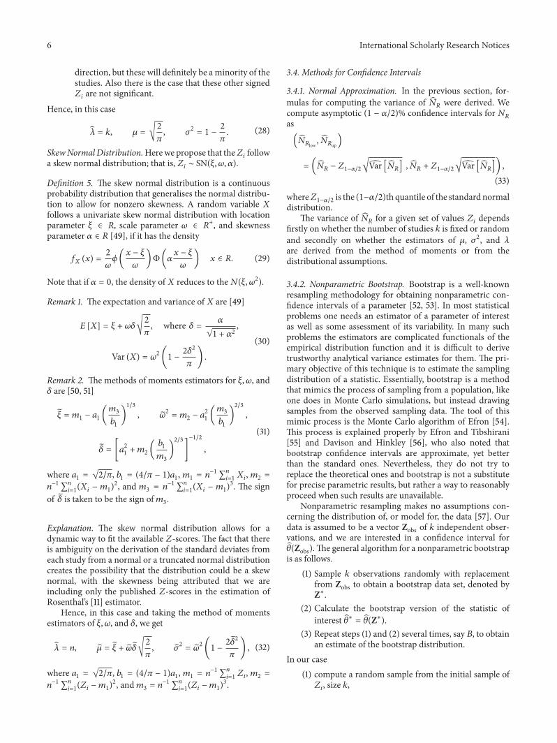
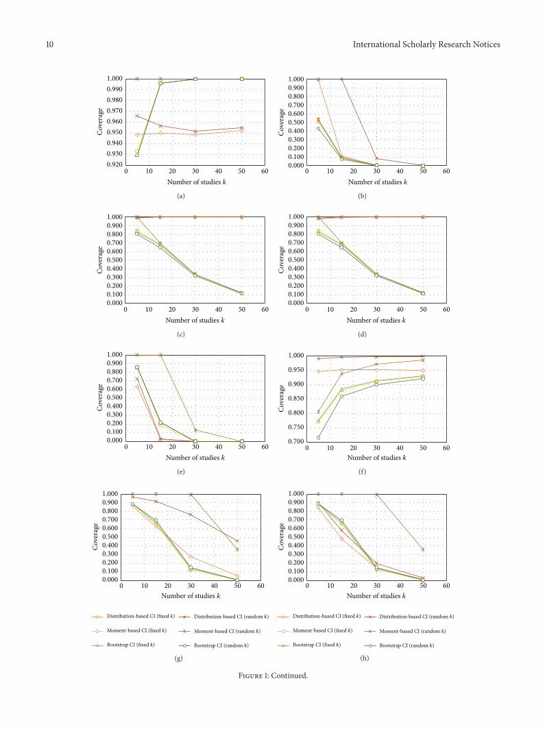
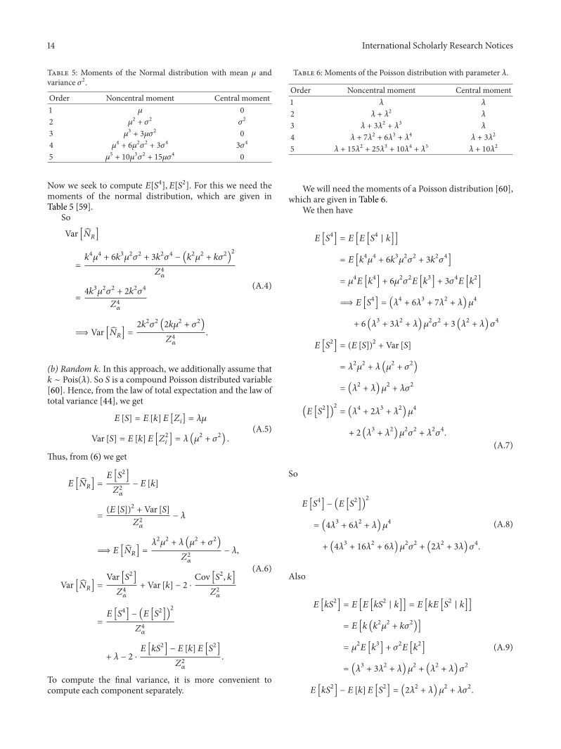may lead to an incorrect usually over optimistic conclusion[10 16] The ability to detect publication bias in a givenfield is a key strength of meta-analysis because identificationof publication bias will challenge the validity of commonviews in that area and will spur further investigations [17]There are two types of statistical procedures for dealing withpublication bias inmeta-analysis methods for identifying theexistence of publication bias and methods for assessing theimpact of publications bias [16] The first includes the funnelplot (and other visualisation methods such as the normalquantile plot) and regressioncorrelation-based tests whilethe second includes the fail-safe (also called file-drawer)number the trim and fill method and selection modelapproaches [10 14 18] Recent approaches include the test forexcess significance [19] and the 119901-curve [20]

Themost commonly usedmethod is the visual inspectionof a funnel plot This assumes that the results from smallerstudies will be more widely spread around the mean effectbecause of larger random error The next most frequentmethod used to assess publication bias is Rosenthalrsquos fail-safenumber [21] Two recent reviews examining the assessmentof publication bias in psychology and ecology reported thatfunnel plots were the most frequently used (24 and 40resp) followed by Rosenthalrsquos fail-safe number (22 and30 resp)

21 Assessing Publication Bias by Computing the Numberof Unpublished Studies Assessing publication bias can beperformed by trying to estimate the number of unpublishedstudies in the given area a meta-analysis is studyingThe fail-safe number represents the number of studies required torefute significant meta-analytic means Although apparentlyintuitive it is in reality difficult to interpret not only becausethe number of data points (ie sample size) for each of 119896 stud-ies is not defined but also because no benchmarks regardingthe fail-safe number exist unlike Cohenrsquos benchmarks foreffect size statistics [22] However these versions have beenheavily criticised mainly because such numbers are oftenmisused and misinterpreted [23] The main reason for thecriticism is that depending on which method is used to esti-mate the fail-safe119873 the number of studies can greatly vary

Although Rosenthalrsquos fail-safe number of publication biaswas proposed as early as 1979 and is frequently cited in theliterature [11] (over 2000 citations) little attention has beengiven to the statistical properties of this estimator This is theaim of the present paper which is discussed in further detailin Section 3

Rosenthal [11] introduced what he called the file drawerproblem His concern was that some statistically nonsignifi-cant studies may be missing from an analysis (ie placed in afile drawer) and that these studies if included would nullifythe observed effect By nullify he meant to reduce the effectto a level not statistically significantly different from zeroRosenthal suggested that rather than speculate on whetherthe file drawer problem existed the actual number of studiesthat would be required to nullify the effect could be calculated[26] This method calculates the significance of multiplestudies by calculating the significance of the mean of thestandard normal deviates of each study Rosenthalrsquos method

calculates the number of additional studies119873119877 with themean

null result necessary to reduce the combined significance toa desired 120572 level (usually 005)

The necessary prerequisite is that each study examines adirectional null hypothesis such that the effect sizes 120579

119894from

each study are examined under 120579119894le 0 or (120579

119894ge 0) Then the

null hypothesis of Stouffer [27] test is

1198670 1205791= sdot sdot sdot = 120579

119896= 0 (1)

The test statistic for this is

119885119878=sum119896

119894=1119885119894

radic119896 (2)

with 119911119894= 120579

119894119904119894 where 119904

119894are the standard errors of 120579

119894 Under

the null hypothesis we have 119885119878sim 119873(0 1) [7]

So we get that the number of additional studies 119873119877

with mean null result necessary to reduce the combinedsignificance to a desired 120572 level (usually 005 [7 11]) is foundafter solving

119885120572=

sum119896

119894=1119885119894

radic119873119877+ 119896

(3)

So119873119877is calculated as

119873119877=(sum

119896

119894=1119885119894)2

1198852120572

minus 119896 (4)

where 119896 is the number of studies and 119885120572is the one-tailed

119885 score associated with the desired 120572 level of significanceRosenthal further suggested that if 119873

119877gt 5119896 + 10 the

likelihood of publication bias would be minimalCooper [28] and Cooper and Rosenthal [29] called this

number the fail-safe sample size or fail-safe number If thisnumber is relatively small then there is cause for concernIf this number is large one might be more confident thatthe effect although possibly inflated by the exclusion ofsome studies is nevertheless not zero [30] This approachis limited in two important ways [26 31] First it assumesthat the association in the hidden studies is zero rather thanconsidering the possibility that some of the studies could havean effect in the reverse direction or an effect that is smallbut not zero Therefore the number of studies required tonullify the effect may be different than the fail-safe numbereither larger or smaller Second this approach focuses onstatistical significance rather than practical or substantivesignificance (effect sizes) That is it may allow one to assertthat the mean correlation is not zero but it does not providean estimate of what the correlation might be (how it haschanged in size) after themissing studies are included [23 32ndash34] However for many fields it remains the gold standard toassess publication bias since its presentation is conceptuallysimple and eloquent In addition it is computationally easyto perform

Iyengar and Greenhouse [12] proposed an alternativeformula for Rosenthalrsquos fail-safe number in which the sumof the unpublished studiesrsquo standard variates is not zero In




119885120572=sum119896

119894=1119885119894+ 119899

120572119872(120572)

radic119899120572+ 119896

(5)

where 119872(120572) = minus120601(119911120572)Φ(119911












119877=(sum

119896

119894=1119885119894)2

1198852120572

minus 119896 (6)


119864[119885119894] = 120583 and Var[119885

119894] = 120590






119894with


119894



next steps

Step 1 1198851 119885

2 119885

119894 119885



119894] = 120583 and Var[119885

119894] = 120590

2Let 119878 = sum

119896



radic119896(119878

119896minus 120583)

119889

997888rarr 119873(0 1205902) 997904rArr 119878

119889

997888rarr 119873(119896120583 1198961205902) (7)


119891119878 (119904) =

1

radic21205871198961205902exp[minus

(119904 minus 119896120583)2

21198961205902] (8)



119878 = 119885120572radic

119877+ 119896 (9)


119877

119878 ge 0 (10)

119877ge 0 (11)






119905


119905)120590

119905)(Φ((119887minus120583

119905)120590

119905)minusΦ((119886 minus 120583

119905)120590

119905))



becomes

119891119878lowast (119904

lowast) =

1


(119904lowastminus 119896120583)

2

21198961205902]

119904lowastge 119885

120572radic119896

(12)



Then we have

119891119877

(119899119877) = 119891

119878lowast (119904

lowast)

10038161003816100381610038161003816100381610038161003816

119889119878lowast

119889119873119877

10038161003816100381610038161003816100381610038161003816

(9)(12)

997904997904997904997904997904rArr 119891119877

(119899119877)

=119885120572

2Φ (120582lowast) radic21205871198961205902 (119899119877 + 119896)

times exp[

[

minus(119885

120572radic119899

119877+ 119896 minus 119896120583)

2

21198961205902]

]

119899119877ge 0

(13)


(119905) = 119864 [exp (119894119905119873119877)]

=Φ ((120583

1+ 120582

lowast) 120590

1)

Φ (120582lowast)

sdot119885120572exp (11989621205832119894119905 (1198852

120572minus 2119896120590

2119894119905) minus 119896119894119905)

(1198852120572minus 21198961205902119894119905)

12

(14)


2

120572minus2119896120590

2119894119905) 1205902

1= 119885

2

120572(119885

2

120572minus

21198961205902119894119905)From (14) we get

119864 [119877] =

11989621205832+ 119896120590

2

1198852120572

minus 119896 + 120576 (15)

where 120576 = (120601(120582lowast)Φ(120582


120572)119885

2

120572)

Also

Var [119877] =

211989621205902(2119896120583

2+ 120590

2)

1198854120572

+ 120575lowast (16)

where

120575lowast=120601 (120582

lowast)

Φ (120582lowast)

[

[

11989621205903(5radic119896120583 + 119885

119886)2

1198854120572

minus(120601 (120582

lowast)

Φ (120582lowast)+ 120582

lowast)119896321205902(radic119896120583 + 119885

119886)2

1198854120572

]

]


Appendix


(13) becomes

119891119877

(119899119877) =

119885120572

2radic21205871198961205902 (119899119877+ 119896)

times exp[

[

minus(119885

120572radic119899

119877+ 119896 minus 119896120583)

2

21198961205902]

]

119899119877ge 0

(18)

Also we get

119864 [119877] =

11989621205832+ 119896120590

2

1198852120572

minus 119896 (19)

Var [119877] =

211989621205902(2119896120583

2+ 120590

2)

1198854120572

(20)




119877for a fixed


119891119877119899(119899119877 119896) = 119891

119877

(119899119877| 119896 = 119896) sdot 119901 (119896 = 119896)

997904rArr 119891119877119899(119899119877 119896)

=119885120572

2Φ (120582lowast) radic21205871198961205902 (119899119877 + 119896)

times exp[

[

minus(119885

120572radic119899

119877+ 119896 minus 119896120583)

2

21198961205902minus 120582]

]

sdot120582119896

119896

119899119877ge 0 119896 = 0 1 2

(21)



119877 This




119864 [119877] =

12058221205832+ 120582 (120583

2+ 120590

2)

1198852120572

minus 120582

Var [119877] = ((4120582

3+ 6120582

2+ 120582) 120583

4

+ (41205823+ 16120582

2+ 6120582) 120583

21205902

+ (21205822+ 3120582) 120590

4)

times (1198854

120572)minus1


2+ 120582) 120583

2+ 120582120590

2

1198852120572

+ 120582

(22)








120583 =sum119896

119894=1119885119894

119896

2=sum119896

119894=11198852

119894

119896minus (

sum119896

119894=1119885119894

119896)

2

(23)


= 119896 120583 =sum119896

119894=1119885119894

119896

2=sum119896

119894=11198852

119894

119896minus (

sum119896

119894=1119885119894

119896)

2

(24)







= 119896 120583 = 0 1205902= 1 (25)






119891and





119891119884(119910) =

1

120590119891radic2120587

exp[

[


119891)2

21205902119891

]

]

+1

120590119891radic2120587

exp[

[


119891)2

21205902119891

]

]

for 119910 ge 0

(26)

(b)

119864 [119884] = 120590119891radic2

120587exp(

minus1205832

119891

21205902119891

) + 120583119891[1 minus 2Φ(

minus120583119891

120590119891

)]

Var [119884]

= 1205832

119891+ 120590

2

119891


120587exp(

minus1205832

119891

21205902119891

) + 120583119891[1 minus 2Φ(

minus120583119891

120590119891

)]

2

(27)



(a) 119891119884(119910) = (radic2120590

119891radic120587) exp (minus119910221205902

119891) for 119910 ge 0

(b) 119864[119884] = 120590119891radic2120587 Var[119884] = 120590

2

119891(1 minus 2120587)


119877are derived







this are as follows



119894gt

1198851205722

or 119885119894lt 119885

1minus1205722occurs


119894can be either










Hence in this case

= 119896 120583 = radic2

120587 120590

2= 1 minus

2

120587 (28)





119891119883 (119909) =

2

120596120601(

119909 minus 120585

120596)Φ(120572

119909 minus 120585

120596) 119909 isin 119877 (29)



119864 [119883] = 120585 + 120596120575radic2

120587 where 120575 = 120572

radic1 + 1205722

Var (119883) = 1205962(1 minus

21205752

120587)

(30)


120585 = 1198981minus 119886

1(1198983

1198871

)

13

2= 119898

2minus 119886

2

1(1198983

1198871

)

23

120575 = [1198862

1+ 119898

2(1198871

1198983

)

23

]

minus12

(31)

where 1198861= radic2120587 119887

1= (4120587 minus 1)119886

1 119898

1= 119899

minus1sum119899

119894=1119883119894 119898

2=

119899minus1sum119899

119894=1(119883

119894minus 119898

1)2 and 119898

3= 119899

minus1sum119899

119894=1(119883

119894minus 119898

1)3 The sign




= 119899 120583 = 120585 + 120575radic2

120587

2=

2(1 minus

21205752

120587) (32)

where 1198861= radic2120587 119887

1= (4120587 minus 1)119886

1 119898

1= 119899

minus1sum119899

119894=1119885119894 119898

2=

119899minus1sum119899

119894=1(119885119894minus 119898

1)2 and119898

3= 119899

minus1sum119899

119894=1(119885119894minus 119898

1)3





as

(119877low

119877up)

= (119877minus 119885


119877]

119877+ 119885


119877])

(33)




119894depends









119885119894 size 119896






119873119877 bootstrap =

sum119873lowast

119877

119887 (34)








ness SN(120575 = 05 120585 = 0 120596 = 1)




119864 [119877] =

11989621205832+ 119896120590

2

1198852120572

minus 119896 (35)


119864 [119877] =

12058221205832+ 120582 (120583

2+ 120590

2)

1198852120572

minus 120582 (36)








distribution HN(01)

5 Examples









simulationplan

Varia

nceformulafor

norm

alapproxim

ationconfi

denceintervals

Bootstr

apconfi

denceinterval

Real

valueo

f119873119877

Distrib

utional

Mom

ents

119896=5153050stu

dies

Draw119885119894fro

mN(01)

HN(01)

SN(120575=minus05120585=0120596=1)

SN(120575=05120585=0120596=1)

Fixed119896(stand

ardno

rmaldistrib


=1halfn

ormal

distr

ibution120583=radic21205871205902


rmalwith

negativ

eskew

ness120583=minusradic121205871205902


rmalwith

positive

skew

ness120583=radic121205871205902

=1minus12120587)

Var[119873119877]=

21198962

1205902

(21198961205832

+1205902

)

1198854 120572

Fixed119896(120583=sum119896 119894=1119885119894

1198961205902

=sum119896 119894=11198852 119894

119896minus(sum119896 119894=1119885119894

119896)

2

)

Var[119873119877]=

21198962

1205902

(21198961205832

+1205902

)

1198854 120572

Usin


compu

tethe119873119877

bootstr

apandrespectiv

elythe

stand

arderrorn

eededto

compu

tethec

onfid

ence

interval

Fixed119896(stand

ardno

rmaldistrib

ution

values120583=01205902

=1halfn

ormal

distr

ibution120583=radic21205871205902

=1minus2120587skew

norm

alwith

negativ

eskewness

120583=minusradic121205871205902


rmal

with

positives


1205902

=1minus12120587)

119864[119873119877]=1198962

1205832

+1198961205902

1198852 120572

minus119896

Rand

om119896(stand

ardno

rmaldistrib


=1half

norm

aldistr

ibution120583=radic21205871205902


rmalwith

negativ



rmalwith

positives

kewness120583=radic121205871205902

=1minus12120587120582=5153050)

Var[119873119877]=

(41205823

+61205822

+120582)1205834

+(41205823

+161205822

+6120582)1205832

1205902

1198854 120572

+

(21205822

+3120582)1205904

1198854 120572

minus2sdot

(21205822

+120582)1205832

+1205821205902

1198852 120572

+120582

Rand

om119896(120583=sum119896 119894=1119885119894

1198961205902

=sum119896 119894=11198852 119894

119896minus(sum119896 119894=1119885119894

119896)

2

120582=5153050)

Var[119873119877]=

(41205823

+61205822

+120582)1205834

+(41205823

+161205822

+6120582)1205832

1205902

1198854 120572

+

(21205822

+3120582)1205904

1198854 120572

minus2sdot

(21205822

+120582)1205832

+1205821205902

1198852 120572

+120582

Usin


compu

tethe119873119877

bootstr

apandrespectiv

elythe

stand

arderrorn

eededto

compu

tethec

onfid

ence

interval

Rand

om119896(stand

ardno

rmaldistrib

ution

values120583=01205902

=1halfn

ormal

distr

ibution120583=radic21205871205902

=1minus2120587skew

norm

alwith

negativ

eskewness

120583=minusradic121205871205902


rmal

with

positives


1205902

=1minus12120587120582=5153050)

119864[119873119877]=

1205822

1205832

+120582(1205832

+1205902

)

1198852 120572

minus120582


Table2Prob

ability

coverage

ofthedifferent

metho

dsforc

onfid

ence

intervals(CI

)according

tothenu

mbero

fstudies119896Th

efig

ureisorganisedas

follo


nfro

mfour

different

distr

ibutions

(stand

ardno

rmaldistr

ibution

halfno

rmaldistr

ibution

skew

norm

alwith

negativ

eskewnessand

skew

norm

alwith

positives

kewness)

Draw119885119894fro

mVa

lues

of120583and1205902fro

mthes

tand

ard

norm

aldistr

ibution

Values

of120583and1205902fro

mthe

halfno

rmaldistr

ibution

HN(01)

Values

of120583and1205902fro

mthe

skew

norm

aldistr

ibution

with

negativ

eskewness

SN(120575=minus05120585=0120596=1)

Values

of120583and1205902fro

mthe

skew

norm

aldistr

ibution

with

positives

kewness

SN(120575=05120585=0120596=1)

119896=5

119896=15119896=30119896=50

119896=5

119896=15119896=30119896=50

119896=5

119896=15119896=30119896=50

119896=5

119896=15119896=30119896=50

Standard

norm

aldistr

ibution

Fixed119896

Distrib

ution

BasedCI

0948

0950

0948

0952

0994

0110

0002

000

00985

0999

1000

1000

0982

0998

1000

1000

Mom

entsBa

sed

CI0933

0996

1000

1000

0529

0088

0005

000

00842

0686

0337

0120

0842

0686

0337

0120

BootstrapCI

0929

0996

1000

1000

0514

0089

0005

000

00830

0680

0337

0120

0830

0680

0337

0120

Rand

om119896

Distrib

ution

BasedCI

0966

0956

0951

0955

0999

1000

0084

0001

0998

1000

1000

1000

0990

0999

1000

1000

Mom

entsBa

sed

CI10

0010

0010

0010

000535

0094

000

6000

010

000702

0338

0122

1000

0702

0338

0122

Bootstr

apCI

0929

0996

1000

1000

0429

0074

000

4000

00804

0649

0322

0115

0804

0649

0322

0115

Halfn

ormaldistr

ibution

HN(01)

Fixed119896

Distrib

ution

BasedCI

0635

0021

000

0000

00945

0952

0951

0948

0864

0624

0279

0053

0841

0483

0142

0014

Mom

entsBa

sed

CI0861

0187

000

0000

00771

0880

0911

0927

0885

0657

0126

0003

0885

0657

0126

0003

Bootstr

apCI

0858

0217

000

0000

00775

0884

0913

0929

0887

0672

0138

0003

0887

0672

0138

0003

Rand

om119896

Distrib

ution

BasedCI

0720

0027

000

0000

00989

0995

0996

0997

0966

0915

0762

0459

0901

0578

0198

0027

Mom

entsBa

sed

CI10

0010

000130

000

00806

0937

0971

0984

1000

1000

0995

0358

1000

1000

0995

0358

Bootstr

apCI

0858

0217

000

0000

00715

0859

0899

0920

0885

0698

0152

000

40885

0698

0152

000

4

Skew

norm

aldistr

ibution

with

negativ

eskewness

SN(120575=minus05120585=0120596=1)

Fixed119896

Distrib

ution

BasedCI

0872

066

60399

0174

0980

0472

0184

004

80953

0970

0977

0981

0944

0948

0949

0957

Mom

entsBa

sed

CI0917

0979

0944

0858

0597

0375

0200

0074

0845

0860

0882

0895

0845

0860

0882

0895

Bootstr

apCI

0912

0978

0945

0857

0586

0377

0199

0074

0840

0857

0881

0894

0840

0857

0881

0894

Rand

om119896

Distrib

ution

BasedCI

0903

0688

040

90178

0996

1000

0687

0306

0987

0997

0998

0999

0965

0964

0965

0968

Mom

entsBa

sed

CI10

0010

000999

0968

060

90399

0237

0103

1000

0872

0886

0902

1000

0872

0886

0902

Bootstr

apCI

0912

0978

0945

0857

0514

0342

0181

006

60818

0845

0874

0889

0818

0845

0874

0889

Skew

norm

aldistr

ibution

with

positives

kewness

SN(120575=05120585=0120596=1)

Fixed119896

Distrib

ution

BasedCI

0880

0673

0402

0164

0982

0471

0186

0050

0956

0972

0976

0979

0948

0952

0951

0955

Mom

entsBa

sed

CI0923

0980

0947

0852

0596

0372

0201

0076

0850

0865

0874

0896

0850

0865

0874

0896

Bootstr

apCI

0918

0978

0946

0846

0583

0372

0200

0077

0841

0862

0873

0896

0841

0862

0873

0896

Rand

om119896

Distrib

ution

BasedCI

0911

0696

0415

0169

0996

1000

0683

0314

0989

0996

0998

0999

0967

0967

0964

0966

Mom

entsBa

sed

CI10

0010

000999

0964

060

60399

0236

0105

1000

0875

0880

0905

1000

0875

0880

0905

Bootstr

apCI

0918

0978

0946

0846

0514

0335

0180

006

80819

0850

0868

0893

0819

0850

0868

0893


092009300940095009600970098009901000

0 10 20 30 40 50 60

Cov

erag

e

Number of studies k

(a)

00000100020003000400050006000700080009001000


Cov

erag

e

(b)

00000100020003000400050006000700080009001000


Cov

erag

e

(c)

00000100020003000400050006000700080009001000


Cov

erag

e

(d)

00000100020003000400050006000700080009001000

0 10 20 30 40 50 60

Cov

erag

e

Number of studies k

(e)

0700

0750

0800

0850

0900

0950

1000


Cov

erag

e

(f)

00000100020003000400050006000700080009001000


Cov

erag

e







(g)

00000100020003000400050006000700080009001000


Cov

erag

e







(h)

Figure 1 Continued


00000100020003000400050006000700080009001000

0 10 20 30 40 50 60

Cov

erag

e

Number of studies k

(i)

00000100020003000400050006000700080009001000


Cov

erag

e

(j)

08000820084008600880090009200940096009801000


Cov

erag

e

(k)

08000820084008600880090009200940096009801000


Cov

erag

e

(l)

00000100020003000400050006000700080009001000

0 10 20 30 40 50 60

Cov

erag

e

Number of studies k

(m)

00000100020003000400050006000700080009001000


Cov

erag

e

(n)

08000820084008600880090009200940096009801000


Cov

erag

e




(o)

08000820084008600880090009200940096009801000


Cov

erag

e




(p)










Momentbased CI


119877= 2124

(2060 2188) (788 3460) (2059 2189) (369 3879) (740 3508)


119877= 73860

(73709 74012) (51618 96102) (73707 74013) (40976 106745) (51662 96059)


1198670 119873

119877le 5119896 + 10

1198671 119873

119877gt 5119896 + 10

(37)


119879amp =119877minus 5119896 minus 10

radicVar [119877]

119889

997888rarr 119873(0 1) (38)



10)radicVar[119877] gt 119885

120572rArr

119877gt 119885

120572radicVar[

119877] + 5119896 + 10




119877








119894119904 The half







Appendices


(a) Fixed 119896 1198851 119885

2 119885

119894 119885



119894] = 120583 and

Var[119885119894] = 120590

2 Let 119878 = sum119896



radic119896(119878

119896minus 120583)

119889

997888rarr 119873(0 1205902) 997904rArr 119878

119889

997888rarr 119873(119896120583 1198961205902) (A1)






So we have

119864 [119878] = 119896120583

Var [119878] = 1198961205902

119864 [1198782] = (119864 [119878])

2+ Var [119878] = 119896

21205832+ 119896120590

2

(A2)


119864 [119877] =

119864 [1198782]

1198852120572

minus 119896 =11989621205832+ 119896120590

2

1198852120572

minus 119896

Var [119877] =

Var [1198782]1198854120572

=119864 [119878

4] minus (119864 [119878

2])2

1198854120572

(A3)




2 1205832+ 120590

21205902

3 1205833+ 3120583120590

20

4 1205834+ 6120583

21205902+ 3120590

43120590

4

5 1205835+ 10120583

31205902+ 15120583120590

40


So

Var [119877]

=11989641205834+ 6119896

312058321205902+ 3119896

21205904minus (119896

21205832+ 119896120590

2)2

1198854120572

=4119896312058321205902+ 2119896

21205904

1198854120572

997904rArr Var [119877] =

211989621205902(2119896120583

2+ 120590

2)

1198854120572

(A4)


119864 [119878] = 119864 [119896] 119864 [119885119894] = 120582120583

Var [119878] = 119864 [119896] 119864 [1198852

119894] = 120582 (120583

2+ 120590

2)

(A5)


119864 [119877] =

119864 [1198782]

1198852120572

minus 119864 [119896]

=(119864 [119878])

2+ Var [119878]1198852120572

minus 120582

997904rArr 119864 [119877] =

12058221205832+ 120582 (120583

2+ 120590

2)

1198852120572

minus 120582

Var [119877] =

Var [1198782]1198854120572


1198852120572

=119864 [119878

4] minus (119864 [119878

2])2

1198854120572

+ 120582 minus 2 sdot119864 [119896119878

2] minus 119864 [119896] 119864 [119878

2]

1198852120572

(A6)




2 120582 + 1205822

120582

3 120582 + 31205822+ 120582

3120582

4 120582 + 71205822+ 6120582

3+ 120582

4120582 + 3120582

2

5 120582 + 151205822+ 25120582

3+ 10120582

4+ 120582

5120582 + 10120582

2


We then have

119864 [1198784] = 119864 [119864 [119878

4| 119896]]

= 119864 [11989641205834+ 6119896

312058321205902+ 3119896

21205904]

= 1205834119864 [119896

4] + 6120583

21205902119864 [119896

3] + 3120590

4119864 [119896

2]

997904rArr 119864 [1198784] = (120582

4+ 6120582

3+ 7120582

2+ 120582) 120583

4

+ 6 (1205823+ 3120582

2+ 120582) 120583

21205902+ 3 (120582

2+ 120582) 120590

4

119864 [1198782] = (119864 [119878])

2+ Var [119878]

= 12058221205832+ 120582 (120583

2+ 120590

2)

= (1205822+ 120582) 120583

2+ 120582120590

2

(119864 [1198782])2

= (1205824+ 2120582

3+ 120582

2) 120583

4

+ 2 (1205823+ 120582

2) 120583

21205902+ 120582

21205904

(A7)

So

119864 [1198784] minus (119864 [119878

2])2

= (41205823+ 6120582

2+ 120582) 120583

4

+ (41205823+ 16120582

2+ 6120582) 120583

21205902+ (2120582

2+ 3120582) 120590

4

(A8)

Also

119864 [1198961198782] = 119864 [119864 [119896119878

2| 119896]] = 119864 [119896119864 [119878

2| 119896]]

= 119864 [119896 (11989621205832+ 119896120590

2)]

= 1205832119864 [119896

3] + 120590

2119864 [119896

2]

= (1205823+ 3120582

2+ 120582) 120583

2+ (120582

2+ 120582) 120590

2

119864 [1198961198782] minus 119864 [119896] 119864 [119878

2] = (2120582

2+ 120582) 120583

2+ 120582120590

2

(A9)



Var [119877] = ((4120582

3+ 6120582

2+ 120582) 120583

4

+ (41205823+ 16120582

2+ 6120582) 120583

21205902

+ (21205822+ 3120582) 120590

4)

times (1198854

120572)minus1


2+ 120582) 120583

2+ 120582120590

2

1198852120572

+ 120582

(A10)



120595119873119877

(119905)

= 119864 [exp (119894119905119873119877)]

= int

+infin

0

exp (119894119905119899119877) 119891

119873119877

(119899119877) 119889119899

119877

= int

+infin

0

119885120572

2Φ (120582lowast) radic21205871198961205902 (119899119877 + 119896)

times exp[

[

119894119905119899119877minus(119885

120572radic119899

119877+ 119896 minus 119896120583)

2

21198961205902]

]

119889119899119877

(let 119908 = 119885120572radic119899

119877+ 119896)

=1


+infin

119885120572radic119896

1

radic21205871198961205902

times exp[119894119905 (1199082

1198852120572


2

21205902]119889119908

(let 119910 =119908 minus 119896120583

radic119899120590)

=1


+infin

minus120582lowast

1

radic2120587

times exp[119894119905 (119896120590

21199102+ 2119899radic119896120583120590119910 + 119896

21205832

1198852120572

minus 119896)

minus1199102

2] 119889119910


int

+infin

minus120582lowast

1

radic2120587

times exp[2119896120590

2119894119905 minus 119885

2

120572

21198852120572

1199102

+2119896radic119896120583120590119894119905

1198852120572

119910 +11989621205832119894119905

1198852120572

]119889119910

(let 1205831=

2119896radic119896120583120590119894119905

1198852120572minus 21198961205902119894119905

1205902

1=

1198852

120572

1198852120572minus 21198961205902119894119905

)


int

+infin

minus120582lowast

1

radic2120587


1)2

212059021

+11989621205832119894119905

1198852120572minus 21198961205902119894119905

] 119889119910

(let 119909 =119910 minus 120583

1

1205901

)

=1205901exp (11989621205832119894119905 (1198852

120572minus 2119896120590

2119894119905) minus 119896119894119905)

Φ (120582lowast)

times int

+infin


1


2

2)119889119909

=119885120572exp (11989621205832119894119905 (1198852

120572minus 2119896120590

2119894119905) minus 119896119894119905)

Φ (120582lowast) (1198852120572minus 21198991205902119894119905)

12


1minus 120582

lowast

1205901

)]

997904rArr 120595119873119877

(119905) =Φ ((120583

1+ 120582

lowast) 120590

1)

Φ (120582lowast)

sdot119885120572exp (11989621205832119894119905 (1198852

120572minus 2120590

2119894119905) minus 119896119894119905)

(1198852120572minus 21198961205902119894119905)

12

(B1)


lowast)120590


1+120582

lowast)120590

1) =

Φ((1205831+ 120582

lowast)120590

1)



119892 (119905) = ln [120595119873119877

(minus119894119905)]

=11989621205832119905

1198852120572minus 21198961205902119905


2ln (1198852

120572minus 2119896120590

2119905)

+ ln [Φ(1205831+ 120582

lowast

1205901

)] + ln119885120572

Φ (120582lowast) 119905 lt

1198852

120572

21198961205902

(C1)


lowast)120590

1 Then

1198921015840(119905) =

119896212058321198852

120572

(1198852120572minus 21198961205902119905)

2minus 119896 +

1198961205902

1198852120572minus 21198961205902119905

+120601 (Δ)

Φ (Δ)Δ1015840

(C2)

with Δ1015840= 2119896radic119896120583120590119885

120572(119885

2

120572minus 2119896120590

2119905)32

minus 1198961205902120582lowast119885

120572(1198852

120572minus

21198961205902119905)12



11989210158401015840(119905) =

41198963120583212059021198852

120572

(1198852120572minus 21198961205902119905)

3+

211989621205904

(1198852120572minus 21198961205902119905)

2

+120601 (Δ)

Φ (Δ)[minus

120601 (Δ)


10158402+ Δ

10158401015840]

(C3)

Then 11989210158401015840(0) leads to (16)



References






































































Volume 2014




Journal of











Journal of


Function Spaces






Algebra












119885120572=sum119896

119894=1119885119894+ 119899

120572119872(120572)

radic119899120572+ 119896

(5)

where 119872(120572) = minus120601(119911120572)Φ(119911












119877=(sum

119896

119894=1119885119894)2

1198852120572

minus 119896 (6)


119864[119885119894] = 120583 and Var[119885

119894] = 120590






119894with


119894



next steps

Step 1 1198851 119885

2 119885

119894 119885



119894] = 120583 and Var[119885

119894] = 120590

2Let 119878 = sum

119896



radic119896(119878

119896minus 120583)

119889

997888rarr 119873(0 1205902) 997904rArr 119878

119889

997888rarr 119873(119896120583 1198961205902) (7)


119891119878 (119904) =

1

radic21205871198961205902exp[minus

(119904 minus 119896120583)2

21198961205902] (8)



119878 = 119885120572radic

119877+ 119896 (9)


119877

119878 ge 0 (10)

119877ge 0 (11)






119905


119905)120590

119905)(Φ((119887minus120583

119905)120590

119905)minusΦ((119886 minus 120583

119905)120590

119905))



becomes

119891119878lowast (119904

lowast) =

1


(119904lowastminus 119896120583)

2

21198961205902]

119904lowastge 119885

120572radic119896

(12)



Then we have

119891119877

(119899119877) = 119891

119878lowast (119904

lowast)

10038161003816100381610038161003816100381610038161003816

119889119878lowast

119889119873119877

10038161003816100381610038161003816100381610038161003816

(9)(12)

997904997904997904997904997904rArr 119891119877

(119899119877)

=119885120572

2Φ (120582lowast) radic21205871198961205902 (119899119877 + 119896)

times exp[

[

minus(119885

120572radic119899

119877+ 119896 minus 119896120583)

2

21198961205902]

]

119899119877ge 0

(13)


(119905) = 119864 [exp (119894119905119873119877)]

=Φ ((120583

1+ 120582

lowast) 120590

1)

Φ (120582lowast)

sdot119885120572exp (11989621205832119894119905 (1198852

120572minus 2119896120590

2119894119905) minus 119896119894119905)

(1198852120572minus 21198961205902119894119905)

12

(14)


2

120572minus2119896120590

2119894119905) 1205902

1= 119885

2

120572(119885

2

120572minus

21198961205902119894119905)From (14) we get

119864 [119877] =

11989621205832+ 119896120590

2

1198852120572

minus 119896 + 120576 (15)

where 120576 = (120601(120582lowast)Φ(120582


120572)119885

2

120572)

Also

Var [119877] =

211989621205902(2119896120583

2+ 120590

2)

1198854120572

+ 120575lowast (16)

where

120575lowast=120601 (120582

lowast)

Φ (120582lowast)

[

[

11989621205903(5radic119896120583 + 119885

119886)2

1198854120572

minus(120601 (120582

lowast)

Φ (120582lowast)+ 120582

lowast)119896321205902(radic119896120583 + 119885

119886)2

1198854120572

]

]


Appendix


(13) becomes

119891119877

(119899119877) =

119885120572

2radic21205871198961205902 (119899119877+ 119896)

times exp[

[

minus(119885

120572radic119899

119877+ 119896 minus 119896120583)

2

21198961205902]

]

119899119877ge 0

(18)

Also we get

119864 [119877] =

11989621205832+ 119896120590

2

1198852120572

minus 119896 (19)

Var [119877] =

211989621205902(2119896120583

2+ 120590

2)

1198854120572

(20)




119877for a fixed


119891119877119899(119899119877 119896) = 119891

119877

(119899119877| 119896 = 119896) sdot 119901 (119896 = 119896)

997904rArr 119891119877119899(119899119877 119896)

=119885120572

2Φ (120582lowast) radic21205871198961205902 (119899119877 + 119896)

times exp[

[

minus(119885

120572radic119899

119877+ 119896 minus 119896120583)

2

21198961205902minus 120582]

]

sdot120582119896

119896

119899119877ge 0 119896 = 0 1 2

(21)



119877 This




119864 [119877] =

12058221205832+ 120582 (120583

2+ 120590

2)

1198852120572

minus 120582

Var [119877] = ((4120582

3+ 6120582

2+ 120582) 120583

4

+ (41205823+ 16120582

2+ 6120582) 120583

21205902

+ (21205822+ 3120582) 120590

4)

times (1198854

120572)minus1


2+ 120582) 120583

2+ 120582120590

2

1198852120572

+ 120582

(22)








120583 =sum119896

119894=1119885119894

119896

2=sum119896

119894=11198852

119894

119896minus (

sum119896

119894=1119885119894

119896)

2

(23)


= 119896 120583 =sum119896

119894=1119885119894

119896

2=sum119896

119894=11198852

119894

119896minus (

sum119896

119894=1119885119894

119896)

2

(24)







= 119896 120583 = 0 1205902= 1 (25)






119891and





119891119884(119910) =

1

120590119891radic2120587

exp[

[


119891)2

21205902119891

]

]

+1

120590119891radic2120587

exp[

[


119891)2

21205902119891

]

]

for 119910 ge 0

(26)

(b)

119864 [119884] = 120590119891radic2

120587exp(

minus1205832

119891

21205902119891

) + 120583119891[1 minus 2Φ(

minus120583119891

120590119891

)]

Var [119884]

= 1205832

119891+ 120590

2

119891


120587exp(

minus1205832

119891

21205902119891

) + 120583119891[1 minus 2Φ(

minus120583119891

120590119891

)]

2

(27)



(a) 119891119884(119910) = (radic2120590

119891radic120587) exp (minus119910221205902

119891) for 119910 ge 0

(b) 119864[119884] = 120590119891radic2120587 Var[119884] = 120590

2

119891(1 minus 2120587)


119877are derived







this are as follows



119894gt

1198851205722

or 119885119894lt 119885

1minus1205722occurs


119894can be either










Hence in this case

= 119896 120583 = radic2

120587 120590

2= 1 minus

2

120587 (28)





119891119883 (119909) =

2

120596120601(

119909 minus 120585

120596)Φ(120572

119909 minus 120585

120596) 119909 isin 119877 (29)



119864 [119883] = 120585 + 120596120575radic2

120587 where 120575 = 120572

radic1 + 1205722

Var (119883) = 1205962(1 minus

21205752

120587)

(30)


120585 = 1198981minus 119886

1(1198983

1198871

)

13

2= 119898

2minus 119886

2

1(1198983

1198871

)

23

120575 = [1198862

1+ 119898

2(1198871

1198983

)

23

]

minus12

(31)

where 1198861= radic2120587 119887

1= (4120587 minus 1)119886

1 119898

1= 119899

minus1sum119899

119894=1119883119894 119898

2=

119899minus1sum119899

119894=1(119883

119894minus 119898

1)2 and 119898

3= 119899

minus1sum119899

119894=1(119883

119894minus 119898

1)3 The sign




= 119899 120583 = 120585 + 120575radic2

120587

2=

2(1 minus

21205752

120587) (32)

where 1198861= radic2120587 119887

1= (4120587 minus 1)119886

1 119898

1= 119899

minus1sum119899

119894=1119885119894 119898

2=

119899minus1sum119899

119894=1(119885119894minus 119898

1)2 and119898

3= 119899

minus1sum119899

119894=1(119885119894minus 119898

1)3





as

(119877low

119877up)

= (119877minus 119885


119877]

119877+ 119885


119877])

(33)




119894depends









119885119894 size 119896






119873119877 bootstrap =

sum119873lowast

119877

119887 (34)








ness SN(120575 = 05 120585 = 0 120596 = 1)




119864 [119877] =

11989621205832+ 119896120590

2

1198852120572

minus 119896 (35)


119864 [119877] =

12058221205832+ 120582 (120583

2+ 120590

2)

1198852120572

minus 120582 (36)








distribution HN(01)

5 Examples









simulationplan

Varia

nceformulafor

norm

alapproxim

ationconfi

denceintervals

Bootstr

apconfi

denceinterval

Real

valueo

f119873119877

Distrib

utional

Mom

ents

119896=5153050stu

dies

Draw119885119894fro

mN(01)

HN(01)

SN(120575=minus05120585=0120596=1)

SN(120575=05120585=0120596=1)

Fixed119896(stand

ardno

rmaldistrib


=1halfn

ormal

distr

ibution120583=radic21205871205902


rmalwith

negativ

eskew

ness120583=minusradic121205871205902


rmalwith

positive

skew

ness120583=radic121205871205902

=1minus12120587)

Var[119873119877]=

21198962

1205902

(21198961205832

+1205902

)

1198854 120572

Fixed119896(120583=sum119896 119894=1119885119894

1198961205902

=sum119896 119894=11198852 119894

119896minus(sum119896 119894=1119885119894

119896)

2

)

Var[119873119877]=

21198962

1205902

(21198961205832

+1205902

)

1198854 120572

Usin


compu

tethe119873119877

bootstr

apandrespectiv

elythe

stand

arderrorn

eededto

compu

tethec

onfid

ence

interval

Fixed119896(stand

ardno

rmaldistrib

ution

values120583=01205902

=1halfn

ormal

distr

ibution120583=radic21205871205902

=1minus2120587skew

norm

alwith

negativ

eskewness

120583=minusradic121205871205902


rmal

with

positives


1205902

=1minus12120587)

119864[119873119877]=1198962

1205832

+1198961205902

1198852 120572

minus119896

Rand

om119896(stand

ardno

rmaldistrib


=1half

norm

aldistr

ibution120583=radic21205871205902


rmalwith

negativ



rmalwith

positives

kewness120583=radic121205871205902

=1minus12120587120582=5153050)

Var[119873119877]=

(41205823

+61205822

+120582)1205834

+(41205823

+161205822

+6120582)1205832

1205902

1198854 120572

+

(21205822

+3120582)1205904

1198854 120572

minus2sdot

(21205822

+120582)1205832

+1205821205902

1198852 120572

+120582

Rand

om119896(120583=sum119896 119894=1119885119894

1198961205902

=sum119896 119894=11198852 119894

119896minus(sum119896 119894=1119885119894

119896)

2

120582=5153050)

Var[119873119877]=

(41205823

+61205822

+120582)1205834

+(41205823

+161205822

+6120582)1205832

1205902

1198854 120572

+

(21205822

+3120582)1205904

1198854 120572

minus2sdot

(21205822

+120582)1205832

+1205821205902

1198852 120572

+120582

Usin


compu

tethe119873119877

bootstr

apandrespectiv

elythe

stand

arderrorn

eededto

compu

tethec

onfid

ence

interval

Rand

om119896(stand

ardno

rmaldistrib

ution

values120583=01205902

=1halfn

ormal

distr

ibution120583=radic21205871205902

=1minus2120587skew

norm

alwith

negativ

eskewness

120583=minusradic121205871205902


rmal

with

positives


1205902

=1minus12120587120582=5153050)

119864[119873119877]=

1205822

1205832

+120582(1205832

+1205902

)

1198852 120572

minus120582


Table2Prob

ability

coverage

ofthedifferent

metho

dsforc

onfid

ence

intervals(CI

)according

tothenu

mbero

fstudies119896Th

efig

ureisorganisedas

follo


nfro

mfour

different

distr

ibutions

(stand

ardno

rmaldistr

ibution

halfno

rmaldistr

ibution

skew

norm

alwith

negativ

eskewnessand

skew

norm

alwith

positives

kewness)

Draw119885119894fro

mVa

lues

of120583and1205902fro

mthes

tand

ard

norm

aldistr

ibution

Values

of120583and1205902fro

mthe

halfno

rmaldistr

ibution

HN(01)

Values

of120583and1205902fro

mthe

skew

norm

aldistr

ibution

with

negativ

eskewness

SN(120575=minus05120585=0120596=1)

Values

of120583and1205902fro

mthe

skew

norm

aldistr

ibution

with

positives

kewness

SN(120575=05120585=0120596=1)

119896=5

119896=15119896=30119896=50

119896=5

119896=15119896=30119896=50

119896=5

119896=15119896=30119896=50

119896=5

119896=15119896=30119896=50

Standard

norm

aldistr

ibution

Fixed119896

Distrib

ution

BasedCI

0948

0950

0948

0952

0994

0110

0002

000

00985

0999

1000

1000

0982

0998

1000

1000

Mom

entsBa

sed

CI0933

0996

1000

1000

0529

0088

0005

000

00842

0686

0337

0120

0842

0686

0337

0120

BootstrapCI

0929

0996

1000

1000

0514

0089

0005

000

00830

0680

0337

0120

0830

0680

0337

0120

Rand

om119896

Distrib

ution

BasedCI

0966

0956

0951

0955

0999

1000

0084

0001

0998

1000

1000

1000

0990

0999

1000

1000

Mom

entsBa

sed

CI10

0010

0010

0010

000535

0094

000

6000

010

000702

0338

0122

1000

0702

0338

0122

Bootstr

apCI

0929

0996

1000

1000

0429

0074

000

4000

00804

0649

0322

0115

0804

0649

0322

0115

Halfn

ormaldistr

ibution

HN(01)

Fixed119896

Distrib

ution

BasedCI

0635

0021

000

0000

00945

0952

0951

0948

0864

0624

0279

0053

0841

0483

0142

0014

Mom

entsBa

sed

CI0861

0187

000

0000

00771

0880

0911

0927

0885

0657

0126

0003

0885

0657

0126

0003

Bootstr

apCI

0858

0217

000

0000

00775

0884

0913

0929

0887

0672

0138

0003

0887

0672

0138

0003

Rand

om119896

Distrib

ution

BasedCI

0720

0027

000

0000

00989

0995

0996

0997

0966

0915

0762

0459

0901

0578

0198

0027

Mom

entsBa

sed

CI10

0010

000130

000

00806

0937

0971

0984

1000

1000

0995

0358

1000

1000

0995

0358

Bootstr

apCI

0858

0217

000

0000

00715

0859

0899

0920

0885

0698

0152

000

40885

0698

0152

000

4

Skew

norm

aldistr

ibution

with

negativ

eskewness

SN(120575=minus05120585=0120596=1)

Fixed119896

Distrib

ution

BasedCI

0872

066

60399

0174

0980

0472

0184

004

80953

0970

0977

0981

0944

0948

0949

0957

Mom

entsBa

sed

CI0917

0979

0944

0858

0597

0375

0200

0074

0845

0860

0882

0895

0845

0860

0882

0895

Bootstr

apCI

0912

0978

0945

0857

0586

0377

0199

0074

0840

0857

0881

0894

0840

0857

0881

0894

Rand

om119896

Distrib

ution

BasedCI

0903

0688

040

90178

0996

1000

0687

0306

0987

0997

0998

0999

0965

0964

0965

0968

Mom

entsBa

sed

CI10

0010

000999

0968

060

90399

0237

0103

1000

0872

0886

0902

1000

0872

0886

0902

Bootstr

apCI

0912

0978

0945

0857

0514

0342

0181

006

60818

0845

0874

0889

0818

0845

0874

0889

Skew

norm

aldistr

ibution

with

positives

kewness

SN(120575=05120585=0120596=1)

Fixed119896

Distrib

ution

BasedCI

0880

0673

0402

0164

0982

0471

0186

0050

0956

0972

0976

0979

0948

0952

0951

0955

Mom

entsBa

sed

CI0923

0980

0947

0852

0596

0372

0201

0076

0850

0865

0874

0896

0850

0865

0874

0896

Bootstr

apCI

0918

0978

0946

0846

0583

0372

0200

0077

0841

0862

0873

0896

0841

0862

0873

0896

Rand

om119896

Distrib

ution

BasedCI

0911

0696

0415

0169

0996

1000

0683

0314

0989

0996

0998

0999

0967

0967

0964

0966

Mom

entsBa

sed

CI10

0010

000999

0964

060

60399

0236

0105

1000

0875

0880

0905

1000

0875

0880

0905

Bootstr

apCI

0918

0978

0946

0846

0514

0335

0180

006

80819

0850

0868

0893

0819

0850

0868

0893


092009300940095009600970098009901000

0 10 20 30 40 50 60

Cov

erag

e

Number of studies k

(a)

00000100020003000400050006000700080009001000


Cov

erag

e

(b)

00000100020003000400050006000700080009001000


Cov

erag

e

(c)

00000100020003000400050006000700080009001000


Cov

erag

e

(d)

00000100020003000400050006000700080009001000

0 10 20 30 40 50 60

Cov

erag

e

Number of studies k

(e)

0700

0750

0800

0850

0900

0950

1000


Cov

erag

e

(f)

00000100020003000400050006000700080009001000


Cov

erag

e







(g)

00000100020003000400050006000700080009001000


Cov

erag

e







(h)

Figure 1 Continued


00000100020003000400050006000700080009001000

0 10 20 30 40 50 60

Cov

erag

e

Number of studies k

(i)

00000100020003000400050006000700080009001000


Cov

erag

e

(j)

08000820084008600880090009200940096009801000


Cov

erag

e

(k)

08000820084008600880090009200940096009801000


Cov

erag

e

(l)

00000100020003000400050006000700080009001000

0 10 20 30 40 50 60

Cov

erag

e

Number of studies k

(m)

00000100020003000400050006000700080009001000


Cov

erag

e

(n)

08000820084008600880090009200940096009801000


Cov

erag

e




(o)

08000820084008600880090009200940096009801000


Cov

erag

e




(p)










Momentbased CI


119877= 2124

(2060 2188) (788 3460) (2059 2189) (369 3879) (740 3508)


119877= 73860

(73709 74012) (51618 96102) (73707 74013) (40976 106745) (51662 96059)


1198670 119873

119877le 5119896 + 10

1198671 119873

119877gt 5119896 + 10

(37)


119879amp =119877minus 5119896 minus 10

radicVar [119877]

119889

997888rarr 119873(0 1) (38)



10)radicVar[119877] gt 119885

120572rArr

119877gt 119885

120572radicVar[

119877] + 5119896 + 10




119877








119894119904 The half







Appendices


(a) Fixed 119896 1198851 119885

2 119885

119894 119885



119894] = 120583 and

Var[119885119894] = 120590

2 Let 119878 = sum119896



radic119896(119878

119896minus 120583)

119889

997888rarr 119873(0 1205902) 997904rArr 119878

119889

997888rarr 119873(119896120583 1198961205902) (A1)






So we have

119864 [119878] = 119896120583

Var [119878] = 1198961205902

119864 [1198782] = (119864 [119878])

2+ Var [119878] = 119896

21205832+ 119896120590

2

(A2)


119864 [119877] =

119864 [1198782]

1198852120572

minus 119896 =11989621205832+ 119896120590

2

1198852120572

minus 119896

Var [119877] =

Var [1198782]1198854120572

=119864 [119878

4] minus (119864 [119878

2])2

1198854120572

(A3)




2 1205832+ 120590

21205902

3 1205833+ 3120583120590

20

4 1205834+ 6120583

21205902+ 3120590

43120590

4

5 1205835+ 10120583

31205902+ 15120583120590

40


So

Var [119877]

=11989641205834+ 6119896

312058321205902+ 3119896

21205904minus (119896

21205832+ 119896120590

2)2

1198854120572

=4119896312058321205902+ 2119896

21205904

1198854120572

997904rArr Var [119877] =

211989621205902(2119896120583

2+ 120590

2)

1198854120572

(A4)


119864 [119878] = 119864 [119896] 119864 [119885119894] = 120582120583

Var [119878] = 119864 [119896] 119864 [1198852

119894] = 120582 (120583

2+ 120590

2)

(A5)


119864 [119877] =

119864 [1198782]

1198852120572

minus 119864 [119896]

=(119864 [119878])

2+ Var [119878]1198852120572

minus 120582

997904rArr 119864 [119877] =

12058221205832+ 120582 (120583

2+ 120590

2)

1198852120572

minus 120582

Var [119877] =

Var [1198782]1198854120572


1198852120572

=119864 [119878

4] minus (119864 [119878

2])2

1198854120572

+ 120582 minus 2 sdot119864 [119896119878

2] minus 119864 [119896] 119864 [119878

2]

1198852120572

(A6)




2 120582 + 1205822

120582

3 120582 + 31205822+ 120582

3120582

4 120582 + 71205822+ 6120582

3+ 120582

4120582 + 3120582

2

5 120582 + 151205822+ 25120582

3+ 10120582

4+ 120582

5120582 + 10120582

2


We then have

119864 [1198784] = 119864 [119864 [119878

4| 119896]]

= 119864 [11989641205834+ 6119896

312058321205902+ 3119896

21205904]

= 1205834119864 [119896

4] + 6120583

21205902119864 [119896

3] + 3120590

4119864 [119896

2]

997904rArr 119864 [1198784] = (120582

4+ 6120582

3+ 7120582

2+ 120582) 120583

4

+ 6 (1205823+ 3120582

2+ 120582) 120583

21205902+ 3 (120582

2+ 120582) 120590

4

119864 [1198782] = (119864 [119878])

2+ Var [119878]

= 12058221205832+ 120582 (120583

2+ 120590

2)

= (1205822+ 120582) 120583

2+ 120582120590

2

(119864 [1198782])2

= (1205824+ 2120582

3+ 120582

2) 120583

4

+ 2 (1205823+ 120582

2) 120583

21205902+ 120582

21205904

(A7)

So

119864 [1198784] minus (119864 [119878

2])2

= (41205823+ 6120582

2+ 120582) 120583

4

+ (41205823+ 16120582

2+ 6120582) 120583

21205902+ (2120582

2+ 3120582) 120590

4

(A8)

Also

119864 [1198961198782] = 119864 [119864 [119896119878

2| 119896]] = 119864 [119896119864 [119878

2| 119896]]

= 119864 [119896 (11989621205832+ 119896120590

2)]

= 1205832119864 [119896

3] + 120590

2119864 [119896

2]

= (1205823+ 3120582

2+ 120582) 120583

2+ (120582

2+ 120582) 120590

2

119864 [1198961198782] minus 119864 [119896] 119864 [119878

2] = (2120582

2+ 120582) 120583

2+ 120582120590

2

(A9)



Var [119877] = ((4120582

3+ 6120582

2+ 120582) 120583

4

+ (41205823+ 16120582

2+ 6120582) 120583

21205902

+ (21205822+ 3120582) 120590

4)

times (1198854

120572)minus1


2+ 120582) 120583

2+ 120582120590

2

1198852120572

+ 120582

(A10)



120595119873119877

(119905)

= 119864 [exp (119894119905119873119877)]

= int

+infin

0

exp (119894119905119899119877) 119891

119873119877

(119899119877) 119889119899

119877

= int

+infin

0

119885120572

2Φ (120582lowast) radic21205871198961205902 (119899119877 + 119896)

times exp[

[

119894119905119899119877minus(119885

120572radic119899

119877+ 119896 minus 119896120583)

2

21198961205902]

]

119889119899119877

(let 119908 = 119885120572radic119899

119877+ 119896)

=1


+infin

119885120572radic119896

1

radic21205871198961205902

times exp[119894119905 (1199082

1198852120572


2

21205902]119889119908

(let 119910 =119908 minus 119896120583

radic119899120590)

=1


+infin

minus120582lowast

1

radic2120587

times exp[119894119905 (119896120590

21199102+ 2119899radic119896120583120590119910 + 119896

21205832

1198852120572

minus 119896)

minus1199102

2] 119889119910


int

+infin

minus120582lowast

1

radic2120587

times exp[2119896120590

2119894119905 minus 119885

2

120572

21198852120572

1199102

+2119896radic119896120583120590119894119905

1198852120572

119910 +11989621205832119894119905

1198852120572

]119889119910

(let 1205831=

2119896radic119896120583120590119894119905

1198852120572minus 21198961205902119894119905

1205902

1=

1198852

120572

1198852120572minus 21198961205902119894119905

)


int

+infin

minus120582lowast

1

radic2120587


1)2

212059021

+11989621205832119894119905

1198852120572minus 21198961205902119894119905

] 119889119910

(let 119909 =119910 minus 120583

1

1205901

)

=1205901exp (11989621205832119894119905 (1198852

120572minus 2119896120590

2119894119905) minus 119896119894119905)

Φ (120582lowast)

times int

+infin


1


2

2)119889119909

=119885120572exp (11989621205832119894119905 (1198852

120572minus 2119896120590

2119894119905) minus 119896119894119905)

Φ (120582lowast) (1198852120572minus 21198991205902119894119905)

12


1minus 120582

lowast

1205901

)]

997904rArr 120595119873119877

(119905) =Φ ((120583

1+ 120582

lowast) 120590

1)

Φ (120582lowast)

sdot119885120572exp (11989621205832119894119905 (1198852

120572minus 2120590

2119894119905) minus 119896119894119905)

(1198852120572minus 21198961205902119894119905)

12

(B1)


lowast)120590


1+120582

lowast)120590

1) =

Φ((1205831+ 120582

lowast)120590

1)



119892 (119905) = ln [120595119873119877

(minus119894119905)]

=11989621205832119905

1198852120572minus 21198961205902119905


2ln (1198852

120572minus 2119896120590

2119905)

+ ln [Φ(1205831+ 120582

lowast

1205901

)] + ln119885120572

Φ (120582lowast) 119905 lt

1198852

120572

21198961205902

(C1)


lowast)120590

1 Then

1198921015840(119905) =

119896212058321198852

120572

(1198852120572minus 21198961205902119905)

2minus 119896 +

1198961205902

1198852120572minus 21198961205902119905

+120601 (Δ)

Φ (Δ)Δ1015840

(C2)

with Δ1015840= 2119896radic119896120583120590119885

120572(119885

2

120572minus 2119896120590

2119905)32

minus 1198961205902120582lowast119885

120572(1198852

120572minus

21198961205902119905)12



11989210158401015840(119905) =

41198963120583212059021198852

120572

(1198852120572minus 21198961205902119905)

3+

211989621205904

(1198852120572minus 21198961205902119905)

2

+120601 (Δ)

Φ (Δ)[minus

120601 (Δ)


10158402+ Δ

10158401015840]

(C3)

Then 11989210158401015840(0) leads to (16)



References






































































Volume 2014




Journal of











Journal of


Function Spaces






Algebra










Then we have

119891119877

(119899119877) = 119891

119878lowast (119904

lowast)

10038161003816100381610038161003816100381610038161003816

119889119878lowast

119889119873119877

10038161003816100381610038161003816100381610038161003816

(9)(12)

997904997904997904997904997904rArr 119891119877

(119899119877)

=119885120572

2Φ (120582lowast) radic21205871198961205902 (119899119877 + 119896)

times exp[

[

minus(119885

120572radic119899

119877+ 119896 minus 119896120583)

2

21198961205902]

]

119899119877ge 0

(13)


(119905) = 119864 [exp (119894119905119873119877)]

=Φ ((120583

1+ 120582

lowast) 120590

1)

Φ (120582lowast)

sdot119885120572exp (11989621205832119894119905 (1198852

120572minus 2119896120590

2119894119905) minus 119896119894119905)

(1198852120572minus 21198961205902119894119905)

12

(14)


2

120572minus2119896120590

2119894119905) 1205902

1= 119885

2

120572(119885

2

120572minus

21198961205902119894119905)From (14) we get

119864 [119877] =

11989621205832+ 119896120590

2

1198852120572

minus 119896 + 120576 (15)

where 120576 = (120601(120582lowast)Φ(120582


120572)119885

2

120572)

Also

Var [119877] =

211989621205902(2119896120583

2+ 120590

2)

1198854120572

+ 120575lowast (16)

where

120575lowast=120601 (120582

lowast)

Φ (120582lowast)

[

[

11989621205903(5radic119896120583 + 119885

119886)2

1198854120572

minus(120601 (120582

lowast)

Φ (120582lowast)+ 120582

lowast)119896321205902(radic119896120583 + 119885

119886)2

1198854120572

]

]


Appendix


(13) becomes

119891119877

(119899119877) =

119885120572

2radic21205871198961205902 (119899119877+ 119896)

times exp[

[

minus(119885

120572radic119899

119877+ 119896 minus 119896120583)

2

21198961205902]

]

119899119877ge 0

(18)

Also we get

119864 [119877] =

11989621205832+ 119896120590

2

1198852120572

minus 119896 (19)

Var [119877] =

211989621205902(2119896120583

2+ 120590

2)

1198854120572

(20)




119877for a fixed


119891119877119899(119899119877 119896) = 119891

119877

(119899119877| 119896 = 119896) sdot 119901 (119896 = 119896)

997904rArr 119891119877119899(119899119877 119896)

=119885120572

2Φ (120582lowast) radic21205871198961205902 (119899119877 + 119896)

times exp[

[

minus(119885

120572radic119899

119877+ 119896 minus 119896120583)

2

21198961205902minus 120582]

]

sdot120582119896

119896

119899119877ge 0 119896 = 0 1 2

(21)



119877 This




119864 [119877] =

12058221205832+ 120582 (120583

2+ 120590

2)

1198852120572

minus 120582

Var [119877] = ((4120582

3+ 6120582

2+ 120582) 120583

4

+ (41205823+ 16120582

2+ 6120582) 120583

21205902

+ (21205822+ 3120582) 120590

4)

times (1198854

120572)minus1


2+ 120582) 120583

2+ 120582120590

2

1198852120572

+ 120582

(22)








120583 =sum119896

119894=1119885119894

119896

2=sum119896

119894=11198852

119894

119896minus (

sum119896

119894=1119885119894

119896)

2

(23)


= 119896 120583 =sum119896

119894=1119885119894

119896

2=sum119896

119894=11198852

119894

119896minus (

sum119896

119894=1119885119894

119896)

2

(24)







= 119896 120583 = 0 1205902= 1 (25)






119891and





119891119884(119910) =

1

120590119891radic2120587

exp[

[


119891)2

21205902119891

]

]

+1

120590119891radic2120587

exp[

[


119891)2

21205902119891

]

]

for 119910 ge 0

(26)

(b)

119864 [119884] = 120590119891radic2

120587exp(

minus1205832

119891

21205902119891

) + 120583119891[1 minus 2Φ(

minus120583119891

120590119891

)]

Var [119884]

= 1205832

119891+ 120590

2

119891


120587exp(

minus1205832

119891

21205902119891

) + 120583119891[1 minus 2Φ(

minus120583119891

120590119891

)]

2

(27)



(a) 119891119884(119910) = (radic2120590

119891radic120587) exp (minus119910221205902

119891) for 119910 ge 0

(b) 119864[119884] = 120590119891radic2120587 Var[119884] = 120590

2

119891(1 minus 2120587)


119877are derived







this are as follows



119894gt

1198851205722

or 119885119894lt 119885

1minus1205722occurs


119894can be either










Hence in this case

= 119896 120583 = radic2

120587 120590

2= 1 minus

2

120587 (28)





119891119883 (119909) =

2

120596120601(

119909 minus 120585

120596)Φ(120572

119909 minus 120585

120596) 119909 isin 119877 (29)



119864 [119883] = 120585 + 120596120575radic2

120587 where 120575 = 120572

radic1 + 1205722

Var (119883) = 1205962(1 minus

21205752

120587)

(30)


120585 = 1198981minus 119886

1(1198983

1198871

)

13

2= 119898

2minus 119886

2

1(1198983

1198871

)

23

120575 = [1198862

1+ 119898

2(1198871

1198983

)

23

]

minus12

(31)

where 1198861= radic2120587 119887

1= (4120587 minus 1)119886

1 119898

1= 119899

minus1sum119899

119894=1119883119894 119898

2=

119899minus1sum119899

119894=1(119883

119894minus 119898

1)2 and 119898

3= 119899

minus1sum119899

119894=1(119883

119894minus 119898

1)3 The sign




= 119899 120583 = 120585 + 120575radic2

120587

2=

2(1 minus

21205752

120587) (32)

where 1198861= radic2120587 119887

1= (4120587 minus 1)119886

1 119898

1= 119899

minus1sum119899

119894=1119885119894 119898

2=

119899minus1sum119899

119894=1(119885119894minus 119898

1)2 and119898

3= 119899

minus1sum119899

119894=1(119885119894minus 119898

1)3





as

(119877low

119877up)

= (119877minus 119885


119877]

119877+ 119885


119877])

(33)




119894depends









119885119894 size 119896






119873119877 bootstrap =

sum119873lowast

119877

119887 (34)








ness SN(120575 = 05 120585 = 0 120596 = 1)




119864 [119877] =

11989621205832+ 119896120590

2

1198852120572

minus 119896 (35)


119864 [119877] =

12058221205832+ 120582 (120583

2+ 120590

2)

1198852120572

minus 120582 (36)








distribution HN(01)

5 Examples









simulationplan

Varia

nceformulafor

norm

alapproxim

ationconfi

denceintervals

Bootstr

apconfi

denceinterval

Real

valueo

f119873119877

Distrib

utional

Mom

ents

119896=5153050stu

dies

Draw119885119894fro

mN(01)

HN(01)

SN(120575=minus05120585=0120596=1)

SN(120575=05120585=0120596=1)

Fixed119896(stand

ardno

rmaldistrib


=1halfn

ormal

distr

ibution120583=radic21205871205902


rmalwith

negativ

eskew

ness120583=minusradic121205871205902


rmalwith

positive

skew

ness120583=radic121205871205902

=1minus12120587)

Var[119873119877]=

21198962

1205902

(21198961205832

+1205902

)

1198854 120572

Fixed119896(120583=sum119896 119894=1119885119894

1198961205902

=sum119896 119894=11198852 119894

119896minus(sum119896 119894=1119885119894

119896)

2

)

Var[119873119877]=

21198962

1205902

(21198961205832

+1205902

)

1198854 120572

Usin


compu

tethe119873119877

bootstr

apandrespectiv

elythe

stand

arderrorn

eededto

compu

tethec

onfid

ence

interval

Fixed119896(stand

ardno

rmaldistrib

ution

values120583=01205902

=1halfn

ormal

distr

ibution120583=radic21205871205902

=1minus2120587skew

norm

alwith

negativ

eskewness

120583=minusradic121205871205902


rmal

with

positives


1205902

=1minus12120587)

119864[119873119877]=1198962

1205832

+1198961205902

1198852 120572

minus119896

Rand

om119896(stand

ardno

rmaldistrib


=1half

norm

aldistr

ibution120583=radic21205871205902


rmalwith

negativ



rmalwith

positives

kewness120583=radic121205871205902

=1minus12120587120582=5153050)

Var[119873119877]=

(41205823

+61205822

+120582)1205834

+(41205823

+161205822

+6120582)1205832

1205902

1198854 120572

+

(21205822

+3120582)1205904

1198854 120572

minus2sdot

(21205822

+120582)1205832

+1205821205902

1198852 120572

+120582

Rand

om119896(120583=sum119896 119894=1119885119894

1198961205902

=sum119896 119894=11198852 119894

119896minus(sum119896 119894=1119885119894

119896)

2

120582=5153050)

Var[119873119877]=

(41205823

+61205822

+120582)1205834

+(41205823

+161205822

+6120582)1205832

1205902

1198854 120572

+

(21205822

+3120582)1205904

1198854 120572

minus2sdot

(21205822

+120582)1205832

+1205821205902

1198852 120572

+120582

Usin


compu

tethe119873119877

bootstr

apandrespectiv

elythe

stand

arderrorn

eededto

compu

tethec

onfid

ence

interval

Rand

om119896(stand

ardno

rmaldistrib

ution

values120583=01205902

=1halfn

ormal

distr

ibution120583=radic21205871205902

=1minus2120587skew

norm

alwith

negativ

eskewness

120583=minusradic121205871205902


rmal

with

positives


1205902

=1minus12120587120582=5153050)

119864[119873119877]=

1205822

1205832

+120582(1205832

+1205902

)

1198852 120572

minus120582


Table2Prob

ability

coverage

ofthedifferent

metho

dsforc

onfid

ence

intervals(CI

)according

tothenu

mbero

fstudies119896Th

efig

ureisorganisedas

follo


nfro

mfour

different

distr

ibutions

(stand

ardno

rmaldistr

ibution

halfno

rmaldistr

ibution

skew

norm

alwith

negativ

eskewnessand

skew

norm

alwith

positives

kewness)

Draw119885119894fro

mVa

lues

of120583and1205902fro

mthes

tand

ard

norm

aldistr

ibution

Values

of120583and1205902fro

mthe

halfno

rmaldistr

ibution

HN(01)

Values

of120583and1205902fro

mthe

skew

norm

aldistr

ibution

with

negativ

eskewness

SN(120575=minus05120585=0120596=1)

Values

of120583and1205902fro

mthe

skew

norm

aldistr

ibution

with

positives

kewness

SN(120575=05120585=0120596=1)

119896=5

119896=15119896=30119896=50

119896=5

119896=15119896=30119896=50

119896=5

119896=15119896=30119896=50

119896=5

119896=15119896=30119896=50

Standard

norm

aldistr

ibution

Fixed119896

Distrib

ution

BasedCI

0948

0950

0948

0952

0994

0110

0002

000

00985

0999

1000

1000

0982

0998

1000

1000

Mom

entsBa

sed

CI0933

0996

1000

1000

0529

0088

0005

000

00842

0686

0337

0120

0842

0686

0337

0120

BootstrapCI

0929

0996

1000

1000

0514

0089

0005

000

00830

0680

0337

0120

0830

0680

0337

0120

Rand

om119896

Distrib

ution

BasedCI

0966

0956

0951

0955

0999

1000

0084

0001

0998

1000

1000

1000

0990

0999

1000

1000

Mom

entsBa

sed

CI10

0010

0010

0010

000535

0094

000

6000

010

000702

0338

0122

1000

0702

0338

0122

Bootstr

apCI

0929

0996

1000

1000

0429

0074

000

4000

00804

0649

0322

0115

0804

0649

0322

0115

Halfn

ormaldistr

ibution

HN(01)

Fixed119896

Distrib

ution

BasedCI

0635

0021

000

0000

00945

0952

0951

0948

0864

0624

0279

0053

0841

0483

0142

0014

Mom

entsBa

sed

CI0861

0187

000

0000

00771

0880

0911

0927

0885

0657

0126

0003

0885

0657

0126

0003

Bootstr

apCI

0858

0217

000

0000

00775

0884

0913

0929

0887

0672

0138

0003

0887

0672

0138

0003

Rand

om119896

Distrib

ution

BasedCI

0720

0027

000

0000

00989

0995

0996

0997

0966

0915

0762

0459

0901

0578

0198

0027

Mom

entsBa

sed

CI10

0010

000130

000

00806

0937

0971

0984

1000

1000

0995

0358

1000

1000

0995

0358

Bootstr

apCI

0858

0217

000

0000

00715

0859

0899

0920

0885

0698

0152

000

40885

0698

0152

000

4

Skew

norm

aldistr

ibution

with

negativ

eskewness

SN(120575=minus05120585=0120596=1)

Fixed119896

Distrib

ution

BasedCI

0872

066

60399

0174

0980

0472

0184

004

80953

0970

0977

0981

0944

0948

0949

0957

Mom

entsBa

sed

CI0917

0979

0944

0858

0597

0375

0200

0074

0845

0860

0882

0895

0845

0860

0882

0895

Bootstr

apCI

0912

0978

0945

0857

0586

0377

0199

0074

0840

0857

0881

0894

0840

0857

0881

0894

Rand

om119896

Distrib

ution

BasedCI

0903

0688

040

90178

0996

1000

0687

0306

0987

0997

0998

0999

0965

0964

0965

0968

Mom

entsBa

sed

CI10

0010

000999

0968

060

90399

0237

0103

1000

0872

0886

0902

1000

0872

0886

0902

Bootstr

apCI

0912

0978

0945

0857

0514

0342

0181

006

60818

0845

0874

0889

0818

0845

0874

0889

Skew

norm

aldistr

ibution

with

positives

kewness

SN(120575=05120585=0120596=1)

Fixed119896

Distrib

ution

BasedCI

0880

0673

0402

0164

0982

0471

0186

0050

0956

0972

0976

0979

0948

0952

0951

0955

Mom

entsBa

sed

CI0923

0980

0947

0852

0596

0372

0201

0076

0850

0865

0874

0896

0850

0865

0874

0896

Bootstr

apCI

0918

0978

0946

0846

0583

0372

0200

0077

0841

0862

0873

0896

0841

0862

0873

0896

Rand

om119896

Distrib

ution

BasedCI

0911

0696

0415

0169

0996

1000

0683

0314

0989

0996

0998

0999

0967

0967

0964

0966

Mom

entsBa

sed

CI10

0010

000999

0964

060

60399

0236

0105

1000

0875

0880

0905

1000

0875

0880

0905

Bootstr

apCI

0918

0978

0946

0846

0514

0335

0180

006

80819

0850

0868

0893

0819

0850

0868

0893


092009300940095009600970098009901000

0 10 20 30 40 50 60

Cov

erag

e

Number of studies k

(a)

00000100020003000400050006000700080009001000


Cov

erag

e

(b)

00000100020003000400050006000700080009001000


Cov

erag

e

(c)

00000100020003000400050006000700080009001000


Cov

erag

e

(d)

00000100020003000400050006000700080009001000

0 10 20 30 40 50 60

Cov

erag

e

Number of studies k

(e)

0700

0750

0800

0850

0900

0950

1000


Cov

erag

e

(f)

00000100020003000400050006000700080009001000


Cov

erag

e







(g)

00000100020003000400050006000700080009001000


Cov

erag

e







(h)

Figure 1 Continued


00000100020003000400050006000700080009001000

0 10 20 30 40 50 60

Cov

erag

e

Number of studies k

(i)

00000100020003000400050006000700080009001000


Cov

erag

e

(j)

08000820084008600880090009200940096009801000


Cov

erag

e

(k)

08000820084008600880090009200940096009801000


Cov

erag

e

(l)

00000100020003000400050006000700080009001000

0 10 20 30 40 50 60

Cov

erag

e

Number of studies k

(m)

00000100020003000400050006000700080009001000


Cov

erag

e

(n)

08000820084008600880090009200940096009801000


Cov

erag

e




(o)

08000820084008600880090009200940096009801000


Cov

erag

e




(p)










Momentbased CI


119877= 2124

(2060 2188) (788 3460) (2059 2189) (369 3879) (740 3508)


119877= 73860

(73709 74012) (51618 96102) (73707 74013) (40976 106745) (51662 96059)


1198670 119873

119877le 5119896 + 10

1198671 119873

119877gt 5119896 + 10

(37)


119879amp =119877minus 5119896 minus 10

radicVar [119877]

119889

997888rarr 119873(0 1) (38)



10)radicVar[119877] gt 119885

120572rArr

119877gt 119885

120572radicVar[

119877] + 5119896 + 10




119877








119894119904 The half







Appendices


(a) Fixed 119896 1198851 119885

2 119885

119894 119885



119894] = 120583 and

Var[119885119894] = 120590

2 Let 119878 = sum119896



radic119896(119878

119896minus 120583)

119889

997888rarr 119873(0 1205902) 997904rArr 119878

119889

997888rarr 119873(119896120583 1198961205902) (A1)






So we have

119864 [119878] = 119896120583

Var [119878] = 1198961205902

119864 [1198782] = (119864 [119878])

2+ Var [119878] = 119896

21205832+ 119896120590

2

(A2)


119864 [119877] =

119864 [1198782]

1198852120572

minus 119896 =11989621205832+ 119896120590

2

1198852120572

minus 119896

Var [119877] =

Var [1198782]1198854120572

=119864 [119878

4] minus (119864 [119878

2])2

1198854120572

(A3)




2 1205832+ 120590

21205902

3 1205833+ 3120583120590

20

4 1205834+ 6120583

21205902+ 3120590

43120590

4

5 1205835+ 10120583

31205902+ 15120583120590

40


So

Var [119877]

=11989641205834+ 6119896

312058321205902+ 3119896

21205904minus (119896

21205832+ 119896120590

2)2

1198854120572

=4119896312058321205902+ 2119896

21205904

1198854120572

997904rArr Var [119877] =

211989621205902(2119896120583

2+ 120590

2)

1198854120572

(A4)


119864 [119878] = 119864 [119896] 119864 [119885119894] = 120582120583

Var [119878] = 119864 [119896] 119864 [1198852

119894] = 120582 (120583

2+ 120590

2)

(A5)


119864 [119877] =

119864 [1198782]

1198852120572

minus 119864 [119896]

=(119864 [119878])

2+ Var [119878]1198852120572

minus 120582

997904rArr 119864 [119877] =

12058221205832+ 120582 (120583

2+ 120590

2)

1198852120572

minus 120582

Var [119877] =

Var [1198782]1198854120572


1198852120572

=119864 [119878

4] minus (119864 [119878

2])2

1198854120572

+ 120582 minus 2 sdot119864 [119896119878

2] minus 119864 [119896] 119864 [119878

2]

1198852120572

(A6)




2 120582 + 1205822

120582

3 120582 + 31205822+ 120582

3120582

4 120582 + 71205822+ 6120582

3+ 120582

4120582 + 3120582

2

5 120582 + 151205822+ 25120582

3+ 10120582

4+ 120582

5120582 + 10120582

2


We then have

119864 [1198784] = 119864 [119864 [119878

4| 119896]]

= 119864 [11989641205834+ 6119896

312058321205902+ 3119896

21205904]

= 1205834119864 [119896

4] + 6120583

21205902119864 [119896

3] + 3120590

4119864 [119896

2]

997904rArr 119864 [1198784] = (120582

4+ 6120582

3+ 7120582

2+ 120582) 120583

4

+ 6 (1205823+ 3120582

2+ 120582) 120583

21205902+ 3 (120582

2+ 120582) 120590

4

119864 [1198782] = (119864 [119878])

2+ Var [119878]

= 12058221205832+ 120582 (120583

2+ 120590

2)

= (1205822+ 120582) 120583

2+ 120582120590

2

(119864 [1198782])2

= (1205824+ 2120582

3+ 120582

2) 120583

4

+ 2 (1205823+ 120582

2) 120583

21205902+ 120582

21205904

(A7)

So

119864 [1198784] minus (119864 [119878

2])2

= (41205823+ 6120582

2+ 120582) 120583

4

+ (41205823+ 16120582

2+ 6120582) 120583

21205902+ (2120582

2+ 3120582) 120590

4

(A8)

Also

119864 [1198961198782] = 119864 [119864 [119896119878

2| 119896]] = 119864 [119896119864 [119878

2| 119896]]

= 119864 [119896 (11989621205832+ 119896120590

2)]

= 1205832119864 [119896

3] + 120590

2119864 [119896

2]

= (1205823+ 3120582

2+ 120582) 120583

2+ (120582

2+ 120582) 120590

2

119864 [1198961198782] minus 119864 [119896] 119864 [119878

2] = (2120582

2+ 120582) 120583

2+ 120582120590

2

(A9)



Var [119877] = ((4120582

3+ 6120582

2+ 120582) 120583

4

+ (41205823+ 16120582

2+ 6120582) 120583

21205902

+ (21205822+ 3120582) 120590

4)

times (1198854

120572)minus1


2+ 120582) 120583

2+ 120582120590

2

1198852120572

+ 120582

(A10)



120595119873119877

(119905)

= 119864 [exp (119894119905119873119877)]

= int

+infin

0

exp (119894119905119899119877) 119891

119873119877

(119899119877) 119889119899

119877

= int

+infin

0

119885120572

2Φ (120582lowast) radic21205871198961205902 (119899119877 + 119896)

times exp[

[

119894119905119899119877minus(119885

120572radic119899

119877+ 119896 minus 119896120583)

2

21198961205902]

]

119889119899119877

(let 119908 = 119885120572radic119899

119877+ 119896)

=1


+infin

119885120572radic119896

1

radic21205871198961205902

times exp[119894119905 (1199082

1198852120572


2

21205902]119889119908

(let 119910 =119908 minus 119896120583

radic119899120590)

=1


+infin

minus120582lowast

1

radic2120587

times exp[119894119905 (119896120590

21199102+ 2119899radic119896120583120590119910 + 119896

21205832

1198852120572

minus 119896)

minus1199102

2] 119889119910


int

+infin

minus120582lowast

1

radic2120587

times exp[2119896120590

2119894119905 minus 119885

2

120572

21198852120572

1199102

+2119896radic119896120583120590119894119905

1198852120572

119910 +11989621205832119894119905

1198852120572

]119889119910

(let 1205831=

2119896radic119896120583120590119894119905

1198852120572minus 21198961205902119894119905

1205902

1=

1198852

120572

1198852120572minus 21198961205902119894119905

)


int

+infin

minus120582lowast

1

radic2120587


1)2

212059021

+11989621205832119894119905

1198852120572minus 21198961205902119894119905

] 119889119910

(let 119909 =119910 minus 120583

1

1205901

)

=1205901exp (11989621205832119894119905 (1198852

120572minus 2119896120590

2119894119905) minus 119896119894119905)

Φ (120582lowast)

times int

+infin


1


2

2)119889119909

=119885120572exp (11989621205832119894119905 (1198852

120572minus 2119896120590

2119894119905) minus 119896119894119905)

Φ (120582lowast) (1198852120572minus 21198991205902119894119905)

12


1minus 120582

lowast

1205901

)]

997904rArr 120595119873119877

(119905) =Φ ((120583

1+ 120582

lowast) 120590

1)

Φ (120582lowast)

sdot119885120572exp (11989621205832119894119905 (1198852

120572minus 2120590

2119894119905) minus 119896119894119905)

(1198852120572minus 21198961205902119894119905)

12

(B1)


lowast)120590


1+120582

lowast)120590

1) =

Φ((1205831+ 120582

lowast)120590

1)



119892 (119905) = ln [120595119873119877

(minus119894119905)]

=11989621205832119905

1198852120572minus 21198961205902119905


2ln (1198852

120572minus 2119896120590

2119905)

+ ln [Φ(1205831+ 120582

lowast

1205901

)] + ln119885120572

Φ (120582lowast) 119905 lt

1198852

120572

21198961205902

(C1)


lowast)120590

1 Then

1198921015840(119905) =

119896212058321198852

120572

(1198852120572minus 21198961205902119905)

2minus 119896 +

1198961205902

1198852120572minus 21198961205902119905

+120601 (Δ)

Φ (Δ)Δ1015840

(C2)

with Δ1015840= 2119896radic119896120583120590119885

120572(119885

2

120572minus 2119896120590

2119905)32

minus 1198961205902120582lowast119885

120572(1198852

120572minus

21198961205902119905)12



11989210158401015840(119905) =

41198963120583212059021198852

120572

(1198852120572minus 21198961205902119905)

3+

211989621205904

(1198852120572minus 21198961205902119905)

2

+120601 (Δ)

Φ (Δ)[minus

120601 (Δ)


10158402+ Δ

10158401015840]

(C3)

Then 11989210158401015840(0) leads to (16)



References






































































Volume 2014




Journal of











Journal of


Function Spaces






Algebra














120583 =sum119896

119894=1119885119894

119896

2=sum119896

119894=11198852

119894

119896minus (

sum119896

119894=1119885119894

119896)

2

(23)


= 119896 120583 =sum119896

119894=1119885119894

119896

2=sum119896

119894=11198852

119894

119896minus (

sum119896

119894=1119885119894

119896)

2

(24)







= 119896 120583 = 0 1205902= 1 (25)






119891and





119891119884(119910) =

1

120590119891radic2120587

exp[

[


119891)2

21205902119891

]

]

+1

120590119891radic2120587

exp[

[


119891)2

21205902119891

]

]

for 119910 ge 0

(26)

(b)

119864 [119884] = 120590119891radic2

120587exp(

minus1205832

119891

21205902119891

) + 120583119891[1 minus 2Φ(

minus120583119891

120590119891

)]

Var [119884]

= 1205832

119891+ 120590

2

119891


120587exp(

minus1205832

119891

21205902119891

) + 120583119891[1 minus 2Φ(

minus120583119891

120590119891

)]

2

(27)



(a) 119891119884(119910) = (radic2120590

119891radic120587) exp (minus119910221205902

119891) for 119910 ge 0

(b) 119864[119884] = 120590119891radic2120587 Var[119884] = 120590

2

119891(1 minus 2120587)


119877are derived







this are as follows



119894gt

1198851205722

or 119885119894lt 119885

1minus1205722occurs


119894can be either










Hence in this case

= 119896 120583 = radic2

120587 120590

2= 1 minus

2

120587 (28)





119891119883 (119909) =

2

120596120601(

119909 minus 120585

120596)Φ(120572

119909 minus 120585

120596) 119909 isin 119877 (29)



119864 [119883] = 120585 + 120596120575radic2

120587 where 120575 = 120572

radic1 + 1205722

Var (119883) = 1205962(1 minus

21205752

120587)

(30)


120585 = 1198981minus 119886

1(1198983

1198871

)

13

2= 119898

2minus 119886

2

1(1198983

1198871

)

23

120575 = [1198862

1+ 119898

2(1198871

1198983

)

23

]

minus12

(31)

where 1198861= radic2120587 119887

1= (4120587 minus 1)119886

1 119898

1= 119899

minus1sum119899

119894=1119883119894 119898

2=

119899minus1sum119899

119894=1(119883

119894minus 119898

1)2 and 119898

3= 119899

minus1sum119899

119894=1(119883

119894minus 119898

1)3 The sign




= 119899 120583 = 120585 + 120575radic2

120587

2=

2(1 minus

21205752

120587) (32)

where 1198861= radic2120587 119887

1= (4120587 minus 1)119886

1 119898

1= 119899

minus1sum119899

119894=1119885119894 119898

2=

119899minus1sum119899

119894=1(119885119894minus 119898

1)2 and119898

3= 119899

minus1sum119899

119894=1(119885119894minus 119898

1)3





as

(119877low

119877up)

= (119877minus 119885


119877]

119877+ 119885


119877])

(33)




119894depends









119885119894 size 119896






119873119877 bootstrap =

sum119873lowast

119877

119887 (34)








ness SN(120575 = 05 120585 = 0 120596 = 1)




119864 [119877] =

11989621205832+ 119896120590

2

1198852120572

minus 119896 (35)


119864 [119877] =

12058221205832+ 120582 (120583

2+ 120590

2)

1198852120572

minus 120582 (36)








distribution HN(01)

5 Examples









simulationplan

Varia

nceformulafor

norm

alapproxim

ationconfi

denceintervals

Bootstr

apconfi

denceinterval

Real

valueo

f119873119877

Distrib

utional

Mom

ents

119896=5153050stu

dies

Draw119885119894fro

mN(01)

HN(01)

SN(120575=minus05120585=0120596=1)

SN(120575=05120585=0120596=1)

Fixed119896(stand

ardno

rmaldistrib


=1halfn

ormal

distr

ibution120583=radic21205871205902


rmalwith

negativ

eskew

ness120583=minusradic121205871205902


rmalwith

positive

skew

ness120583=radic121205871205902

=1minus12120587)

Var[119873119877]=

21198962

1205902

(21198961205832

+1205902

)

1198854 120572

Fixed119896(120583=sum119896 119894=1119885119894

1198961205902

=sum119896 119894=11198852 119894

119896minus(sum119896 119894=1119885119894

119896)

2

)

Var[119873119877]=

21198962

1205902

(21198961205832

+1205902

)

1198854 120572

Usin


compu

tethe119873119877

bootstr

apandrespectiv

elythe

stand

arderrorn

eededto

compu

tethec

onfid

ence

interval

Fixed119896(stand

ardno

rmaldistrib

ution

values120583=01205902

=1halfn

ormal

distr

ibution120583=radic21205871205902

=1minus2120587skew

norm

alwith

negativ

eskewness

120583=minusradic121205871205902


rmal

with

positives


1205902

=1minus12120587)

119864[119873119877]=1198962

1205832

+1198961205902

1198852 120572

minus119896

Rand

om119896(stand

ardno

rmaldistrib


=1half

norm

aldistr

ibution120583=radic21205871205902


rmalwith

negativ



rmalwith

positives

kewness120583=radic121205871205902

=1minus12120587120582=5153050)

Var[119873119877]=

(41205823

+61205822

+120582)1205834

+(41205823

+161205822

+6120582)1205832

1205902

1198854 120572

+

(21205822

+3120582)1205904

1198854 120572

minus2sdot

(21205822

+120582)1205832

+1205821205902

1198852 120572

+120582

Rand

om119896(120583=sum119896 119894=1119885119894

1198961205902

=sum119896 119894=11198852 119894

119896minus(sum119896 119894=1119885119894

119896)

2

120582=5153050)

Var[119873119877]=

(41205823

+61205822

+120582)1205834

+(41205823

+161205822

+6120582)1205832

1205902

1198854 120572

+

(21205822

+3120582)1205904

1198854 120572

minus2sdot

(21205822

+120582)1205832

+1205821205902

1198852 120572

+120582

Usin


compu

tethe119873119877

bootstr

apandrespectiv

elythe

stand

arderrorn

eededto

compu

tethec

onfid

ence

interval

Rand

om119896(stand

ardno

rmaldistrib

ution

values120583=01205902

=1halfn

ormal

distr

ibution120583=radic21205871205902

=1minus2120587skew

norm

alwith

negativ

eskewness

120583=minusradic121205871205902


rmal

with

positives


1205902

=1minus12120587120582=5153050)

119864[119873119877]=

1205822

1205832

+120582(1205832

+1205902

)

1198852 120572

minus120582


Table2Prob

ability

coverage

ofthedifferent

metho

dsforc

onfid

ence

intervals(CI

)according

tothenu

mbero

fstudies119896Th

efig

ureisorganisedas

follo


nfro

mfour

different

distr

ibutions

(stand

ardno

rmaldistr

ibution

halfno

rmaldistr

ibution

skew

norm

alwith

negativ

eskewnessand

skew

norm

alwith

positives

kewness)

Draw119885119894fro

mVa

lues

of120583and1205902fro

mthes

tand

ard

norm

aldistr

ibution

Values

of120583and1205902fro

mthe

halfno

rmaldistr

ibution

HN(01)

Values

of120583and1205902fro

mthe

skew

norm

aldistr

ibution

with

negativ

eskewness

SN(120575=minus05120585=0120596=1)

Values

of120583and1205902fro

mthe

skew

norm

aldistr

ibution

with

positives

kewness

SN(120575=05120585=0120596=1)

119896=5

119896=15119896=30119896=50

119896=5

119896=15119896=30119896=50

119896=5

119896=15119896=30119896=50

119896=5

119896=15119896=30119896=50

Standard

norm

aldistr

ibution

Fixed119896

Distrib

ution

BasedCI

0948

0950

0948

0952

0994

0110

0002

000

00985

0999

1000

1000

0982

0998

1000

1000

Mom

entsBa

sed

CI0933

0996

1000

1000

0529

0088

0005

000

00842

0686

0337

0120

0842

0686

0337

0120

BootstrapCI

0929

0996

1000

1000

0514

0089

0005

000

00830

0680

0337

0120

0830

0680

0337

0120

Rand

om119896

Distrib

ution

BasedCI

0966

0956

0951

0955

0999

1000

0084

0001

0998

1000

1000

1000

0990

0999

1000

1000

Mom

entsBa

sed

CI10

0010

0010

0010

000535

0094

000

6000

010

000702

0338

0122

1000

0702

0338

0122

Bootstr

apCI

0929

0996

1000

1000

0429

0074

000

4000

00804

0649

0322

0115

0804

0649

0322

0115

Halfn

ormaldistr

ibution

HN(01)

Fixed119896

Distrib

ution

BasedCI

0635

0021

000

0000

00945

0952

0951

0948

0864

0624

0279

0053

0841

0483

0142

0014

Mom

entsBa

sed

CI0861

0187

000

0000

00771

0880

0911

0927

0885

0657

0126

0003

0885

0657

0126

0003

Bootstr

apCI

0858

0217

000

0000

00775

0884

0913

0929

0887

0672

0138

0003

0887

0672

0138

0003

Rand

om119896

Distrib

ution

BasedCI

0720

0027

000

0000

00989

0995

0996

0997

0966

0915

0762

0459

0901

0578

0198

0027

Mom

entsBa

sed

CI10

0010

000130

000

00806

0937

0971

0984

1000

1000

0995

0358

1000

1000

0995

0358

Bootstr

apCI

0858

0217

000

0000

00715

0859

0899

0920

0885

0698

0152

000

40885

0698

0152

000

4

Skew

norm

aldistr

ibution

with

negativ

eskewness

SN(120575=minus05120585=0120596=1)

Fixed119896

Distrib

ution

BasedCI

0872

066

60399

0174

0980

0472

0184

004

80953

0970

0977

0981

0944

0948

0949

0957

Mom

entsBa

sed

CI0917

0979

0944

0858

0597

0375

0200

0074

0845

0860

0882

0895

0845

0860

0882

0895

Bootstr

apCI

0912

0978

0945

0857

0586

0377

0199

0074

0840

0857

0881

0894

0840

0857

0881

0894

Rand

om119896

Distrib

ution

BasedCI

0903

0688

040

90178

0996

1000

0687

0306

0987

0997

0998

0999

0965

0964

0965

0968

Mom

entsBa

sed

CI10

0010

000999

0968

060

90399

0237

0103

1000

0872

0886

0902

1000

0872

0886

0902

Bootstr

apCI

0912

0978

0945

0857

0514

0342

0181

006

60818

0845

0874

0889

0818

0845

0874

0889

Skew

norm

aldistr

ibution

with

positives

kewness

SN(120575=05120585=0120596=1)

Fixed119896

Distrib

ution

BasedCI

0880

0673

0402

0164

0982

0471

0186

0050

0956

0972

0976

0979

0948

0952

0951

0955

Mom

entsBa

sed

CI0923

0980

0947

0852

0596

0372

0201

0076

0850

0865

0874

0896

0850

0865

0874

0896

Bootstr

apCI

0918

0978

0946

0846

0583

0372

0200

0077

0841

0862

0873

0896

0841

0862

0873

0896

Rand

om119896

Distrib

ution

BasedCI

0911

0696

0415

0169

0996

1000

0683

0314

0989

0996

0998

0999

0967

0967

0964

0966

Mom

entsBa

sed

CI10

0010

000999

0964

060

60399

0236

0105

1000

0875

0880

0905

1000

0875

0880

0905

Bootstr

apCI

0918

0978

0946

0846

0514

0335

0180

006

80819

0850

0868

0893

0819

0850

0868

0893


092009300940095009600970098009901000

0 10 20 30 40 50 60

Cov

erag

e

Number of studies k

(a)

00000100020003000400050006000700080009001000


Cov

erag

e

(b)

00000100020003000400050006000700080009001000


Cov

erag

e

(c)

00000100020003000400050006000700080009001000


Cov

erag

e

(d)

00000100020003000400050006000700080009001000

0 10 20 30 40 50 60

Cov

erag

e

Number of studies k

(e)

0700

0750

0800

0850

0900

0950

1000


Cov

erag

e

(f)

00000100020003000400050006000700080009001000


Cov

erag

e







(g)

00000100020003000400050006000700080009001000


Cov

erag

e







(h)

Figure 1 Continued


00000100020003000400050006000700080009001000

0 10 20 30 40 50 60

Cov

erag

e

Number of studies k

(i)

00000100020003000400050006000700080009001000


Cov

erag

e

(j)

08000820084008600880090009200940096009801000


Cov

erag

e

(k)

08000820084008600880090009200940096009801000


Cov

erag

e

(l)

00000100020003000400050006000700080009001000

0 10 20 30 40 50 60

Cov

erag

e

Number of studies k

(m)

00000100020003000400050006000700080009001000


Cov

erag

e

(n)

08000820084008600880090009200940096009801000


Cov

erag

e




(o)

08000820084008600880090009200940096009801000


Cov

erag

e




(p)










Momentbased CI


119877= 2124

(2060 2188) (788 3460) (2059 2189) (369 3879) (740 3508)


119877= 73860

(73709 74012) (51618 96102) (73707 74013) (40976 106745) (51662 96059)


1198670 119873

119877le 5119896 + 10

1198671 119873

119877gt 5119896 + 10

(37)


119879amp =119877minus 5119896 minus 10

radicVar [119877]

119889

997888rarr 119873(0 1) (38)



10)radicVar[119877] gt 119885

120572rArr

119877gt 119885

120572radicVar[

119877] + 5119896 + 10




119877








119894119904 The half







Appendices


(a) Fixed 119896 1198851 119885

2 119885

119894 119885



119894] = 120583 and

Var[119885119894] = 120590

2 Let 119878 = sum119896



radic119896(119878

119896minus 120583)

119889

997888rarr 119873(0 1205902) 997904rArr 119878

119889

997888rarr 119873(119896120583 1198961205902) (A1)






So we have

119864 [119878] = 119896120583

Var [119878] = 1198961205902

119864 [1198782] = (119864 [119878])

2+ Var [119878] = 119896

21205832+ 119896120590

2

(A2)


119864 [119877] =

119864 [1198782]

1198852120572

minus 119896 =11989621205832+ 119896120590

2

1198852120572

minus 119896

Var [119877] =

Var [1198782]1198854120572

=119864 [119878

4] minus (119864 [119878

2])2

1198854120572

(A3)




2 1205832+ 120590

21205902

3 1205833+ 3120583120590

20

4 1205834+ 6120583

21205902+ 3120590

43120590

4

5 1205835+ 10120583

31205902+ 15120583120590

40


So

Var [119877]

=11989641205834+ 6119896

312058321205902+ 3119896

21205904minus (119896

21205832+ 119896120590

2)2

1198854120572

=4119896312058321205902+ 2119896

21205904

1198854120572

997904rArr Var [119877] =

211989621205902(2119896120583

2+ 120590

2)

1198854120572

(A4)


119864 [119878] = 119864 [119896] 119864 [119885119894] = 120582120583

Var [119878] = 119864 [119896] 119864 [1198852

119894] = 120582 (120583

2+ 120590

2)

(A5)


119864 [119877] =

119864 [1198782]

1198852120572

minus 119864 [119896]

=(119864 [119878])

2+ Var [119878]1198852120572

minus 120582

997904rArr 119864 [119877] =

12058221205832+ 120582 (120583

2+ 120590

2)

1198852120572

minus 120582

Var [119877] =

Var [1198782]1198854120572


1198852120572

=119864 [119878

4] minus (119864 [119878

2])2

1198854120572

+ 120582 minus 2 sdot119864 [119896119878

2] minus 119864 [119896] 119864 [119878

2]

1198852120572

(A6)




2 120582 + 1205822

120582

3 120582 + 31205822+ 120582

3120582

4 120582 + 71205822+ 6120582

3+ 120582

4120582 + 3120582

2

5 120582 + 151205822+ 25120582

3+ 10120582

4+ 120582

5120582 + 10120582

2


We then have

119864 [1198784] = 119864 [119864 [119878

4| 119896]]

= 119864 [11989641205834+ 6119896

312058321205902+ 3119896

21205904]

= 1205834119864 [119896

4] + 6120583

21205902119864 [119896

3] + 3120590

4119864 [119896

2]

997904rArr 119864 [1198784] = (120582

4+ 6120582

3+ 7120582

2+ 120582) 120583

4

+ 6 (1205823+ 3120582

2+ 120582) 120583

21205902+ 3 (120582

2+ 120582) 120590

4

119864 [1198782] = (119864 [119878])

2+ Var [119878]

= 12058221205832+ 120582 (120583

2+ 120590

2)

= (1205822+ 120582) 120583

2+ 120582120590

2

(119864 [1198782])2

= (1205824+ 2120582

3+ 120582

2) 120583

4

+ 2 (1205823+ 120582

2) 120583

21205902+ 120582

21205904

(A7)

So

119864 [1198784] minus (119864 [119878

2])2

= (41205823+ 6120582

2+ 120582) 120583

4

+ (41205823+ 16120582

2+ 6120582) 120583

21205902+ (2120582

2+ 3120582) 120590

4

(A8)

Also

119864 [1198961198782] = 119864 [119864 [119896119878

2| 119896]] = 119864 [119896119864 [119878

2| 119896]]

= 119864 [119896 (11989621205832+ 119896120590

2)]

= 1205832119864 [119896

3] + 120590

2119864 [119896

2]

= (1205823+ 3120582

2+ 120582) 120583

2+ (120582

2+ 120582) 120590

2

119864 [1198961198782] minus 119864 [119896] 119864 [119878

2] = (2120582

2+ 120582) 120583

2+ 120582120590

2

(A9)



Var [119877] = ((4120582

3+ 6120582

2+ 120582) 120583

4

+ (41205823+ 16120582

2+ 6120582) 120583

21205902

+ (21205822+ 3120582) 120590

4)

times (1198854

120572)minus1


2+ 120582) 120583

2+ 120582120590

2

1198852120572

+ 120582

(A10)



120595119873119877

(119905)

= 119864 [exp (119894119905119873119877)]

= int

+infin

0

exp (119894119905119899119877) 119891

119873119877

(119899119877) 119889119899

119877

= int

+infin

0

119885120572

2Φ (120582lowast) radic21205871198961205902 (119899119877 + 119896)

times exp[

[

119894119905119899119877minus(119885

120572radic119899

119877+ 119896 minus 119896120583)

2

21198961205902]

]

119889119899119877

(let 119908 = 119885120572radic119899

119877+ 119896)

=1


+infin

119885120572radic119896

1

radic21205871198961205902

times exp[119894119905 (1199082

1198852120572


2

21205902]119889119908

(let 119910 =119908 minus 119896120583

radic119899120590)

=1


+infin

minus120582lowast

1

radic2120587

times exp[119894119905 (119896120590

21199102+ 2119899radic119896120583120590119910 + 119896

21205832

1198852120572

minus 119896)

minus1199102

2] 119889119910


int

+infin

minus120582lowast

1

radic2120587

times exp[2119896120590

2119894119905 minus 119885

2

120572

21198852120572

1199102

+2119896radic119896120583120590119894119905

1198852120572

119910 +11989621205832119894119905

1198852120572

]119889119910

(let 1205831=

2119896radic119896120583120590119894119905

1198852120572minus 21198961205902119894119905

1205902

1=

1198852

120572

1198852120572minus 21198961205902119894119905

)


int

+infin

minus120582lowast

1

radic2120587


1)2

212059021

+11989621205832119894119905

1198852120572minus 21198961205902119894119905

] 119889119910

(let 119909 =119910 minus 120583

1

1205901

)

=1205901exp (11989621205832119894119905 (1198852

120572minus 2119896120590

2119894119905) minus 119896119894119905)

Φ (120582lowast)

times int

+infin


1


2

2)119889119909

=119885120572exp (11989621205832119894119905 (1198852

120572minus 2119896120590

2119894119905) minus 119896119894119905)

Φ (120582lowast) (1198852120572minus 21198991205902119894119905)

12


1minus 120582

lowast

1205901

)]

997904rArr 120595119873119877

(119905) =Φ ((120583

1+ 120582

lowast) 120590

1)

Φ (120582lowast)

sdot119885120572exp (11989621205832119894119905 (1198852

120572minus 2120590

2119894119905) minus 119896119894119905)

(1198852120572minus 21198961205902119894119905)

12

(B1)


lowast)120590


1+120582

lowast)120590

1) =

Φ((1205831+ 120582

lowast)120590

1)



119892 (119905) = ln [120595119873119877

(minus119894119905)]

=11989621205832119905

1198852120572minus 21198961205902119905


2ln (1198852

120572minus 2119896120590

2119905)

+ ln [Φ(1205831+ 120582

lowast

1205901

)] + ln119885120572

Φ (120582lowast) 119905 lt

1198852

120572

21198961205902

(C1)


lowast)120590

1 Then

1198921015840(119905) =

119896212058321198852

120572

(1198852120572minus 21198961205902119905)

2minus 119896 +

1198961205902

1198852120572minus 21198961205902119905

+120601 (Δ)

Φ (Δ)Δ1015840

(C2)

with Δ1015840= 2119896radic119896120583120590119885

120572(119885

2

120572minus 2119896120590

2119905)32

minus 1198961205902120582lowast119885

120572(1198852

120572minus

21198961205902119905)12



11989210158401015840(119905) =

41198963120583212059021198852

120572

(1198852120572minus 21198961205902119905)

3+

211989621205904

(1198852120572minus 21198961205902119905)

2

+120601 (Δ)

Φ (Δ)[minus

120601 (Δ)


10158402+ Δ

10158401015840]

(C3)

Then 11989210158401015840(0) leads to (16)



References






































































Volume 2014




Journal of











Journal of


Function Spaces






Algebra











Hence in this case

= 119896 120583 = radic2

120587 120590

2= 1 minus

2

120587 (28)





119891119883 (119909) =

2

120596120601(

119909 minus 120585

120596)Φ(120572

119909 minus 120585

120596) 119909 isin 119877 (29)



119864 [119883] = 120585 + 120596120575radic2

120587 where 120575 = 120572

radic1 + 1205722

Var (119883) = 1205962(1 minus

21205752

120587)

(30)


120585 = 1198981minus 119886

1(1198983

1198871

)

13

2= 119898

2minus 119886

2

1(1198983

1198871

)

23

120575 = [1198862

1+ 119898

2(1198871

1198983

)

23

]

minus12

(31)

where 1198861= radic2120587 119887

1= (4120587 minus 1)119886

1 119898

1= 119899

minus1sum119899

119894=1119883119894 119898

2=

119899minus1sum119899

119894=1(119883

119894minus 119898

1)2 and 119898

3= 119899

minus1sum119899

119894=1(119883

119894minus 119898

1)3 The sign




= 119899 120583 = 120585 + 120575radic2

120587

2=

2(1 minus

21205752

120587) (32)

where 1198861= radic2120587 119887

1= (4120587 minus 1)119886

1 119898

1= 119899

minus1sum119899

119894=1119885119894 119898

2=

119899minus1sum119899

119894=1(119885119894minus 119898

1)2 and119898

3= 119899

minus1sum119899

119894=1(119885119894minus 119898

1)3





as

(119877low

119877up)

= (119877minus 119885


119877]

119877+ 119885


119877])

(33)




119894depends









119885119894 size 119896






119873119877 bootstrap =

sum119873lowast

119877

119887 (34)








ness SN(120575 = 05 120585 = 0 120596 = 1)




119864 [119877] =

11989621205832+ 119896120590

2

1198852120572

minus 119896 (35)


119864 [119877] =

12058221205832+ 120582 (120583

2+ 120590

2)

1198852120572

minus 120582 (36)








distribution HN(01)

5 Examples









simulationplan

Varia

nceformulafor

norm

alapproxim

ationconfi

denceintervals

Bootstr

apconfi

denceinterval

Real

valueo

f119873119877

Distrib

utional

Mom

ents

119896=5153050stu

dies

Draw119885119894fro

mN(01)

HN(01)

SN(120575=minus05120585=0120596=1)

SN(120575=05120585=0120596=1)

Fixed119896(stand

ardno

rmaldistrib


=1halfn

ormal

distr

ibution120583=radic21205871205902


rmalwith

negativ

eskew

ness120583=minusradic121205871205902


rmalwith

positive

skew

ness120583=radic121205871205902

=1minus12120587)

Var[119873119877]=

21198962

1205902

(21198961205832

+1205902

)

1198854 120572

Fixed119896(120583=sum119896 119894=1119885119894

1198961205902

=sum119896 119894=11198852 119894

119896minus(sum119896 119894=1119885119894

119896)

2

)

Var[119873119877]=

21198962

1205902

(21198961205832

+1205902

)

1198854 120572

Usin


compu

tethe119873119877

bootstr

apandrespectiv

elythe

stand

arderrorn

eededto

compu

tethec

onfid

ence

interval

Fixed119896(stand

ardno

rmaldistrib

ution

values120583=01205902

=1halfn

ormal

distr

ibution120583=radic21205871205902

=1minus2120587skew

norm

alwith

negativ

eskewness

120583=minusradic121205871205902


rmal

with

positives


1205902

=1minus12120587)

119864[119873119877]=1198962

1205832

+1198961205902

1198852 120572

minus119896

Rand

om119896(stand

ardno

rmaldistrib


=1half

norm

aldistr

ibution120583=radic21205871205902


rmalwith

negativ



rmalwith

positives

kewness120583=radic121205871205902

=1minus12120587120582=5153050)

Var[119873119877]=

(41205823

+61205822

+120582)1205834

+(41205823

+161205822

+6120582)1205832

1205902

1198854 120572

+

(21205822

+3120582)1205904

1198854 120572

minus2sdot

(21205822

+120582)1205832

+1205821205902

1198852 120572

+120582

Rand

om119896(120583=sum119896 119894=1119885119894

1198961205902

=sum119896 119894=11198852 119894

119896minus(sum119896 119894=1119885119894

119896)

2

120582=5153050)

Var[119873119877]=

(41205823

+61205822

+120582)1205834

+(41205823

+161205822

+6120582)1205832

1205902

1198854 120572

+

(21205822

+3120582)1205904

1198854 120572

minus2sdot

(21205822

+120582)1205832

+1205821205902

1198852 120572

+120582

Usin


compu

tethe119873119877

bootstr

apandrespectiv

elythe

stand

arderrorn

eededto

compu

tethec

onfid

ence

interval

Rand

om119896(stand

ardno

rmaldistrib

ution

values120583=01205902

=1halfn

ormal

distr

ibution120583=radic21205871205902

=1minus2120587skew

norm

alwith

negativ

eskewness

120583=minusradic121205871205902


rmal

with

positives


1205902

=1minus12120587120582=5153050)

119864[119873119877]=

1205822

1205832

+120582(1205832

+1205902

)

1198852 120572

minus120582


Table2Prob

ability

coverage

ofthedifferent

metho

dsforc

onfid

ence

intervals(CI

)according

tothenu

mbero

fstudies119896Th

efig

ureisorganisedas

follo


nfro

mfour

different

distr

ibutions

(stand

ardno

rmaldistr

ibution

halfno

rmaldistr

ibution

skew

norm

alwith

negativ

eskewnessand

skew

norm

alwith

positives

kewness)

Draw119885119894fro

mVa

lues

of120583and1205902fro

mthes

tand

ard

norm

aldistr

ibution

Values

of120583and1205902fro

mthe

halfno

rmaldistr

ibution

HN(01)

Values

of120583and1205902fro

mthe

skew

norm

aldistr

ibution

with

negativ

eskewness

SN(120575=minus05120585=0120596=1)

Values

of120583and1205902fro

mthe

skew

norm

aldistr

ibution

with

positives

kewness

SN(120575=05120585=0120596=1)

119896=5

119896=15119896=30119896=50

119896=5

119896=15119896=30119896=50

119896=5

119896=15119896=30119896=50

119896=5

119896=15119896=30119896=50

Standard

norm

aldistr

ibution

Fixed119896

Distrib

ution

BasedCI

0948

0950

0948

0952

0994

0110

0002

000

00985

0999

1000

1000

0982

0998

1000

1000

Mom

entsBa

sed

CI0933

0996

1000

1000

0529

0088

0005

000

00842

0686

0337

0120

0842

0686

0337

0120

BootstrapCI

0929

0996

1000

1000

0514

0089

0005

000

00830

0680

0337

0120

0830

0680

0337

0120

Rand

om119896

Distrib

ution

BasedCI

0966

0956

0951

0955

0999

1000

0084

0001

0998

1000

1000

1000

0990

0999

1000

1000

Mom

entsBa

sed

CI10

0010

0010

0010

000535

0094

000

6000

010

000702

0338

0122

1000

0702

0338

0122

Bootstr

apCI

0929

0996

1000

1000

0429

0074

000

4000

00804

0649

0322

0115

0804

0649

0322

0115

Halfn

ormaldistr

ibution

HN(01)

Fixed119896

Distrib

ution

BasedCI

0635

0021

000

0000

00945

0952

0951

0948

0864

0624

0279

0053

0841

0483

0142

0014

Mom

entsBa

sed

CI0861

0187

000

0000

00771

0880

0911

0927

0885

0657

0126

0003

0885

0657

0126

0003

Bootstr

apCI

0858

0217

000

0000

00775

0884

0913

0929

0887

0672

0138

0003

0887

0672

0138

0003

Rand

om119896

Distrib

ution

BasedCI

0720

0027

000

0000

00989

0995

0996

0997

0966

0915

0762

0459

0901

0578

0198

0027

Mom

entsBa

sed

CI10

0010

000130

000

00806

0937

0971

0984

1000

1000

0995

0358

1000

1000

0995

0358

Bootstr

apCI

0858

0217

000

0000

00715

0859

0899

0920

0885

0698

0152

000

40885

0698

0152

000

4

Skew

norm

aldistr

ibution

with

negativ

eskewness

SN(120575=minus05120585=0120596=1)

Fixed119896

Distrib

ution

BasedCI

0872

066

60399

0174

0980

0472

0184

004

80953

0970

0977

0981

0944

0948

0949

0957

Mom

entsBa

sed

CI0917

0979

0944

0858

0597

0375

0200

0074

0845

0860

0882

0895

0845

0860

0882

0895

Bootstr

apCI

0912

0978

0945

0857

0586

0377

0199

0074

0840

0857

0881

0894

0840

0857

0881

0894

Rand

om119896

Distrib

ution

BasedCI

0903

0688

040

90178

0996

1000

0687

0306

0987

0997

0998

0999

0965

0964

0965

0968

Mom

entsBa

sed

CI10

0010

000999

0968

060

90399

0237

0103

1000

0872

0886

0902

1000

0872

0886

0902

Bootstr

apCI

0912

0978

0945

0857

0514

0342

0181

006

60818

0845

0874

0889

0818

0845

0874

0889

Skew

norm

aldistr

ibution

with

positives

kewness

SN(120575=05120585=0120596=1)

Fixed119896

Distrib

ution

BasedCI

0880

0673

0402

0164

0982

0471

0186

0050

0956

0972

0976

0979

0948

0952

0951

0955

Mom

entsBa

sed

CI0923

0980

0947

0852

0596

0372

0201

0076

0850

0865

0874

0896

0850

0865

0874

0896

Bootstr

apCI

0918

0978

0946

0846

0583

0372

0200

0077

0841

0862

0873

0896

0841

0862

0873

0896

Rand

om119896

Distrib

ution

BasedCI

0911

0696

0415

0169

0996

1000

0683

0314

0989

0996

0998

0999

0967

0967

0964

0966

Mom

entsBa

sed

CI10

0010

000999

0964

060

60399

0236

0105

1000

0875

0880

0905

1000

0875

0880

0905

Bootstr

apCI

0918

0978

0946

0846

0514

0335

0180

006

80819

0850

0868

0893

0819

0850

0868

0893


092009300940095009600970098009901000

0 10 20 30 40 50 60

Cov

erag

e

Number of studies k

(a)

00000100020003000400050006000700080009001000


Cov

erag

e

(b)

00000100020003000400050006000700080009001000


Cov

erag

e

(c)

00000100020003000400050006000700080009001000


Cov

erag

e

(d)

00000100020003000400050006000700080009001000

0 10 20 30 40 50 60

Cov

erag

e

Number of studies k

(e)

0700

0750

0800

0850

0900

0950

1000


Cov

erag

e

(f)

00000100020003000400050006000700080009001000


Cov

erag

e







(g)

00000100020003000400050006000700080009001000


Cov

erag

e







(h)

Figure 1 Continued


00000100020003000400050006000700080009001000

0 10 20 30 40 50 60

Cov

erag

e

Number of studies k

(i)

00000100020003000400050006000700080009001000


Cov

erag

e

(j)

08000820084008600880090009200940096009801000


Cov

erag

e

(k)

08000820084008600880090009200940096009801000


Cov

erag

e

(l)

00000100020003000400050006000700080009001000

0 10 20 30 40 50 60

Cov

erag

e

Number of studies k

(m)

00000100020003000400050006000700080009001000


Cov

erag

e

(n)

08000820084008600880090009200940096009801000


Cov

erag

e




(o)

08000820084008600880090009200940096009801000


Cov

erag

e




(p)










Momentbased CI


119877= 2124

(2060 2188) (788 3460) (2059 2189) (369 3879) (740 3508)


119877= 73860

(73709 74012) (51618 96102) (73707 74013) (40976 106745) (51662 96059)


1198670 119873

119877le 5119896 + 10

1198671 119873

119877gt 5119896 + 10

(37)


119879amp =119877minus 5119896 minus 10

radicVar [119877]

119889

997888rarr 119873(0 1) (38)



10)radicVar[119877] gt 119885

120572rArr

119877gt 119885

120572radicVar[

119877] + 5119896 + 10




119877








119894119904 The half







Appendices


(a) Fixed 119896 1198851 119885

2 119885

119894 119885



119894] = 120583 and

Var[119885119894] = 120590

2 Let 119878 = sum119896



radic119896(119878

119896minus 120583)

119889

997888rarr 119873(0 1205902) 997904rArr 119878

119889

997888rarr 119873(119896120583 1198961205902) (A1)






So we have

119864 [119878] = 119896120583

Var [119878] = 1198961205902

119864 [1198782] = (119864 [119878])

2+ Var [119878] = 119896

21205832+ 119896120590

2

(A2)


119864 [119877] =

119864 [1198782]

1198852120572

minus 119896 =11989621205832+ 119896120590

2

1198852120572

minus 119896

Var [119877] =

Var [1198782]1198854120572

=119864 [119878

4] minus (119864 [119878

2])2

1198854120572

(A3)




2 1205832+ 120590

21205902

3 1205833+ 3120583120590

20

4 1205834+ 6120583

21205902+ 3120590

43120590

4

5 1205835+ 10120583

31205902+ 15120583120590

40


So

Var [119877]

=11989641205834+ 6119896

312058321205902+ 3119896

21205904minus (119896

21205832+ 119896120590

2)2

1198854120572

=4119896312058321205902+ 2119896

21205904

1198854120572

997904rArr Var [119877] =

211989621205902(2119896120583

2+ 120590

2)

1198854120572

(A4)


119864 [119878] = 119864 [119896] 119864 [119885119894] = 120582120583

Var [119878] = 119864 [119896] 119864 [1198852

119894] = 120582 (120583

2+ 120590

2)

(A5)


119864 [119877] =

119864 [1198782]

1198852120572

minus 119864 [119896]

=(119864 [119878])

2+ Var [119878]1198852120572

minus 120582

997904rArr 119864 [119877] =

12058221205832+ 120582 (120583

2+ 120590

2)

1198852120572

minus 120582

Var [119877] =

Var [1198782]1198854120572


1198852120572

=119864 [119878

4] minus (119864 [119878

2])2

1198854120572

+ 120582 minus 2 sdot119864 [119896119878

2] minus 119864 [119896] 119864 [119878

2]

1198852120572

(A6)




2 120582 + 1205822

120582

3 120582 + 31205822+ 120582

3120582

4 120582 + 71205822+ 6120582

3+ 120582

4120582 + 3120582

2

5 120582 + 151205822+ 25120582

3+ 10120582

4+ 120582

5120582 + 10120582

2


We then have

119864 [1198784] = 119864 [119864 [119878

4| 119896]]

= 119864 [11989641205834+ 6119896

312058321205902+ 3119896

21205904]

= 1205834119864 [119896

4] + 6120583

21205902119864 [119896

3] + 3120590

4119864 [119896

2]

997904rArr 119864 [1198784] = (120582

4+ 6120582

3+ 7120582

2+ 120582) 120583

4

+ 6 (1205823+ 3120582

2+ 120582) 120583

21205902+ 3 (120582

2+ 120582) 120590

4

119864 [1198782] = (119864 [119878])

2+ Var [119878]

= 12058221205832+ 120582 (120583

2+ 120590

2)

= (1205822+ 120582) 120583

2+ 120582120590

2

(119864 [1198782])2

= (1205824+ 2120582

3+ 120582

2) 120583

4

+ 2 (1205823+ 120582

2) 120583

21205902+ 120582

21205904

(A7)

So

119864 [1198784] minus (119864 [119878

2])2

= (41205823+ 6120582

2+ 120582) 120583

4

+ (41205823+ 16120582

2+ 6120582) 120583

21205902+ (2120582

2+ 3120582) 120590

4

(A8)

Also

119864 [1198961198782] = 119864 [119864 [119896119878

2| 119896]] = 119864 [119896119864 [119878

2| 119896]]

= 119864 [119896 (11989621205832+ 119896120590

2)]

= 1205832119864 [119896

3] + 120590

2119864 [119896

2]

= (1205823+ 3120582

2+ 120582) 120583

2+ (120582

2+ 120582) 120590

2

119864 [1198961198782] minus 119864 [119896] 119864 [119878

2] = (2120582

2+ 120582) 120583

2+ 120582120590

2

(A9)



Var [119877] = ((4120582

3+ 6120582

2+ 120582) 120583

4

+ (41205823+ 16120582

2+ 6120582) 120583

21205902

+ (21205822+ 3120582) 120590

4)

times (1198854

120572)minus1


2+ 120582) 120583

2+ 120582120590

2

1198852120572

+ 120582

(A10)



120595119873119877

(119905)

= 119864 [exp (119894119905119873119877)]

= int

+infin

0

exp (119894119905119899119877) 119891

119873119877

(119899119877) 119889119899

119877

= int

+infin

0

119885120572

2Φ (120582lowast) radic21205871198961205902 (119899119877 + 119896)

times exp[

[

119894119905119899119877minus(119885

120572radic119899

119877+ 119896 minus 119896120583)

2

21198961205902]

]

119889119899119877

(let 119908 = 119885120572radic119899

119877+ 119896)

=1


+infin

119885120572radic119896

1

radic21205871198961205902

times exp[119894119905 (1199082

1198852120572


2

21205902]119889119908

(let 119910 =119908 minus 119896120583

radic119899120590)

=1


+infin

minus120582lowast

1

radic2120587

times exp[119894119905 (119896120590

21199102+ 2119899radic119896120583120590119910 + 119896

21205832

1198852120572

minus 119896)

minus1199102

2] 119889119910


int

+infin

minus120582lowast

1

radic2120587

times exp[2119896120590

2119894119905 minus 119885

2

120572

21198852120572

1199102

+2119896radic119896120583120590119894119905

1198852120572

119910 +11989621205832119894119905

1198852120572

]119889119910

(let 1205831=

2119896radic119896120583120590119894119905

1198852120572minus 21198961205902119894119905

1205902

1=

1198852

120572

1198852120572minus 21198961205902119894119905

)


int

+infin

minus120582lowast

1

radic2120587


1)2

212059021

+11989621205832119894119905

1198852120572minus 21198961205902119894119905

] 119889119910

(let 119909 =119910 minus 120583

1

1205901

)

=1205901exp (11989621205832119894119905 (1198852

120572minus 2119896120590

2119894119905) minus 119896119894119905)

Φ (120582lowast)

times int

+infin


1


2

2)119889119909

=119885120572exp (11989621205832119894119905 (1198852

120572minus 2119896120590

2119894119905) minus 119896119894119905)

Φ (120582lowast) (1198852120572minus 21198991205902119894119905)

12


1minus 120582

lowast

1205901

)]

997904rArr 120595119873119877

(119905) =Φ ((120583

1+ 120582

lowast) 120590

1)

Φ (120582lowast)

sdot119885120572exp (11989621205832119894119905 (1198852

120572minus 2120590

2119894119905) minus 119896119894119905)

(1198852120572minus 21198961205902119894119905)

12

(B1)


lowast)120590


1+120582

lowast)120590

1) =

Φ((1205831+ 120582

lowast)120590

1)



119892 (119905) = ln [120595119873119877

(minus119894119905)]

=11989621205832119905

1198852120572minus 21198961205902119905


2ln (1198852

120572minus 2119896120590

2119905)

+ ln [Φ(1205831+ 120582

lowast

1205901

)] + ln119885120572

Φ (120582lowast) 119905 lt

1198852

120572

21198961205902

(C1)


lowast)120590

1 Then

1198921015840(119905) =

119896212058321198852

120572

(1198852120572minus 21198961205902119905)

2minus 119896 +

1198961205902

1198852120572minus 21198961205902119905

+120601 (Δ)

Φ (Δ)Δ1015840

(C2)

with Δ1015840= 2119896radic119896120583120590119885

120572(119885

2

120572minus 2119896120590

2119905)32

minus 1198961205902120582lowast119885

120572(1198852

120572minus

21198961205902119905)12



11989210158401015840(119905) =

41198963120583212059021198852

120572

(1198852120572minus 21198961205902119905)

3+

211989621205904

(1198852120572minus 21198961205902119905)

2

+120601 (Δ)

Φ (Δ)[minus

120601 (Δ)


10158402+ Δ

10158401015840]

(C3)

Then 11989210158401015840(0) leads to (16)



References






































































Volume 2014




Journal of











Journal of


Function Spaces






Algebra














119873119877 bootstrap =

sum119873lowast

119877

119887 (34)








ness SN(120575 = 05 120585 = 0 120596 = 1)




119864 [119877] =

11989621205832+ 119896120590

2

1198852120572

minus 119896 (35)


119864 [119877] =

12058221205832+ 120582 (120583

2+ 120590

2)

1198852120572

minus 120582 (36)








distribution HN(01)

5 Examples









simulationplan

Varia

nceformulafor

norm

alapproxim

ationconfi

denceintervals

Bootstr

apconfi

denceinterval

Real

valueo

f119873119877

Distrib

utional

Mom

ents

119896=5153050stu

dies

Draw119885119894fro

mN(01)

HN(01)

SN(120575=minus05120585=0120596=1)

SN(120575=05120585=0120596=1)

Fixed119896(stand

ardno

rmaldistrib


=1halfn

ormal

distr

ibution120583=radic21205871205902


rmalwith

negativ

eskew

ness120583=minusradic121205871205902


rmalwith

positive

skew

ness120583=radic121205871205902

=1minus12120587)

Var[119873119877]=

21198962

1205902

(21198961205832

+1205902

)

1198854 120572

Fixed119896(120583=sum119896 119894=1119885119894

1198961205902

=sum119896 119894=11198852 119894

119896minus(sum119896 119894=1119885119894

119896)

2

)

Var[119873119877]=

21198962

1205902

(21198961205832

+1205902

)

1198854 120572

Usin


compu

tethe119873119877

bootstr

apandrespectiv

elythe

stand

arderrorn

eededto

compu

tethec

onfid

ence

interval

Fixed119896(stand

ardno

rmaldistrib

ution

values120583=01205902

=1halfn

ormal

distr

ibution120583=radic21205871205902

=1minus2120587skew

norm

alwith

negativ

eskewness

120583=minusradic121205871205902


rmal

with

positives


1205902

=1minus12120587)

119864[119873119877]=1198962

1205832

+1198961205902

1198852 120572

minus119896

Rand

om119896(stand

ardno

rmaldistrib


=1half

norm

aldistr

ibution120583=radic21205871205902


rmalwith

negativ



rmalwith

positives

kewness120583=radic121205871205902

=1minus12120587120582=5153050)

Var[119873119877]=

(41205823

+61205822

+120582)1205834

+(41205823

+161205822

+6120582)1205832

1205902

1198854 120572

+

(21205822

+3120582)1205904

1198854 120572

minus2sdot

(21205822

+120582)1205832

+1205821205902

1198852 120572

+120582

Rand

om119896(120583=sum119896 119894=1119885119894

1198961205902

=sum119896 119894=11198852 119894

119896minus(sum119896 119894=1119885119894

119896)

2

120582=5153050)

Var[119873119877]=

(41205823

+61205822

+120582)1205834

+(41205823

+161205822

+6120582)1205832

1205902

1198854 120572

+

(21205822

+3120582)1205904

1198854 120572

minus2sdot

(21205822

+120582)1205832

+1205821205902

1198852 120572

+120582

Usin


compu

tethe119873119877

bootstr

apandrespectiv

elythe

stand

arderrorn

eededto

compu

tethec

onfid

ence

interval

Rand

om119896(stand

ardno

rmaldistrib

ution

values120583=01205902

=1halfn

ormal

distr

ibution120583=radic21205871205902

=1minus2120587skew

norm

alwith

negativ

eskewness

120583=minusradic121205871205902


rmal

with

positives


1205902

=1minus12120587120582=5153050)

119864[119873119877]=

1205822

1205832

+120582(1205832

+1205902

)

1198852 120572

minus120582


Table2Prob

ability

coverage

ofthedifferent

metho

dsforc

onfid

ence

intervals(CI

)according

tothenu

mbero

fstudies119896Th

efig

ureisorganisedas

follo


nfro

mfour

different

distr

ibutions

(stand

ardno

rmaldistr

ibution

halfno

rmaldistr

ibution

skew

norm

alwith

negativ

eskewnessand

skew

norm

alwith

positives

kewness)

Draw119885119894fro

mVa

lues

of120583and1205902fro

mthes

tand

ard

norm

aldistr

ibution

Values

of120583and1205902fro

mthe

halfno

rmaldistr

ibution

HN(01)

Values

of120583and1205902fro

mthe

skew

norm

aldistr

ibution

with

negativ

eskewness

SN(120575=minus05120585=0120596=1)

Values

of120583and1205902fro

mthe

skew

norm

aldistr

ibution

with

positives

kewness

SN(120575=05120585=0120596=1)

119896=5

119896=15119896=30119896=50

119896=5

119896=15119896=30119896=50

119896=5

119896=15119896=30119896=50

119896=5

119896=15119896=30119896=50

Standard

norm

aldistr

ibution

Fixed119896

Distrib

ution

BasedCI

0948

0950

0948

0952

0994

0110

0002

000

00985

0999

1000

1000

0982

0998

1000

1000

Mom

entsBa

sed

CI0933

0996

1000

1000

0529

0088

0005

000

00842

0686

0337

0120

0842

0686

0337

0120

BootstrapCI

0929

0996

1000

1000

0514

0089

0005

000

00830

0680

0337

0120

0830

0680

0337

0120

Rand

om119896

Distrib

ution

BasedCI

0966

0956

0951

0955

0999

1000

0084

0001

0998

1000

1000

1000

0990

0999

1000

1000

Mom

entsBa

sed

CI10

0010

0010

0010

000535

0094

000

6000

010

000702

0338

0122

1000

0702

0338

0122

Bootstr

apCI

0929

0996

1000

1000

0429

0074

000

4000

00804

0649

0322

0115

0804

0649

0322

0115

Halfn

ormaldistr

ibution

HN(01)

Fixed119896

Distrib

ution

BasedCI

0635

0021

000

0000

00945

0952

0951

0948

0864

0624

0279

0053

0841

0483

0142

0014

Mom

entsBa

sed

CI0861

0187

000

0000

00771

0880

0911

0927

0885

0657

0126

0003

0885

0657

0126

0003

Bootstr

apCI

0858

0217

000

0000

00775

0884

0913

0929

0887

0672

0138

0003

0887

0672

0138

0003

Rand

om119896

Distrib

ution

BasedCI

0720

0027

000

0000

00989

0995

0996

0997

0966

0915

0762

0459

0901

0578

0198

0027

Mom

entsBa

sed

CI10

0010

000130

000

00806

0937

0971

0984

1000

1000

0995

0358

1000

1000

0995

0358

Bootstr

apCI

0858

0217

000

0000

00715

0859

0899

0920

0885

0698

0152

000

40885

0698

0152

000

4

Skew

norm

aldistr

ibution

with

negativ

eskewness

SN(120575=minus05120585=0120596=1)

Fixed119896

Distrib

ution

BasedCI

0872

066

60399

0174

0980

0472

0184

004

80953

0970

0977

0981

0944

0948

0949

0957

Mom

entsBa

sed

CI0917

0979

0944

0858

0597

0375

0200

0074

0845

0860

0882

0895

0845

0860

0882

0895

Bootstr

apCI

0912

0978

0945

0857

0586

0377

0199

0074

0840

0857

0881

0894

0840

0857

0881

0894

Rand

om119896

Distrib

ution

BasedCI

0903

0688

040

90178

0996

1000

0687

0306

0987

0997

0998

0999

0965

0964

0965

0968

Mom

entsBa

sed

CI10

0010

000999

0968

060

90399

0237

0103

1000

0872

0886

0902

1000

0872

0886

0902

Bootstr

apCI

0912

0978

0945

0857

0514

0342

0181

006

60818

0845

0874

0889

0818

0845

0874

0889

Skew

norm

aldistr

ibution

with

positives

kewness

SN(120575=05120585=0120596=1)

Fixed119896

Distrib

ution

BasedCI

0880

0673

0402

0164

0982

0471

0186

0050

0956

0972

0976

0979

0948

0952

0951

0955

Mom

entsBa

sed

CI0923

0980

0947

0852

0596

0372

0201

0076

0850

0865

0874

0896

0850

0865

0874

0896

Bootstr

apCI

0918

0978

0946

0846

0583

0372

0200

0077

0841

0862

0873

0896

0841

0862

0873

0896

Rand

om119896

Distrib

ution

BasedCI

0911

0696

0415

0169

0996

1000

0683

0314

0989

0996

0998

0999

0967

0967

0964

0966

Mom

entsBa

sed

CI10

0010

000999

0964

060

60399

0236

0105

1000

0875

0880

0905

1000

0875

0880

0905

Bootstr

apCI

0918

0978

0946

0846

0514

0335

0180

006

80819

0850

0868

0893

0819

0850

0868

0893


092009300940095009600970098009901000

0 10 20 30 40 50 60

Cov

erag

e

Number of studies k

(a)

00000100020003000400050006000700080009001000


Cov

erag

e

(b)

00000100020003000400050006000700080009001000


Cov

erag

e

(c)

00000100020003000400050006000700080009001000


Cov

erag

e

(d)

00000100020003000400050006000700080009001000

0 10 20 30 40 50 60

Cov

erag

e

Number of studies k

(e)

0700

0750

0800

0850

0900

0950

1000


Cov

erag

e

(f)

00000100020003000400050006000700080009001000


Cov

erag

e







(g)

00000100020003000400050006000700080009001000


Cov

erag

e







(h)

Figure 1 Continued


00000100020003000400050006000700080009001000

0 10 20 30 40 50 60

Cov

erag

e

Number of studies k

(i)

00000100020003000400050006000700080009001000


Cov

erag

e

(j)

08000820084008600880090009200940096009801000


Cov

erag

e

(k)

08000820084008600880090009200940096009801000


Cov

erag

e

(l)

00000100020003000400050006000700080009001000

0 10 20 30 40 50 60

Cov

erag

e

Number of studies k

(m)

00000100020003000400050006000700080009001000


Cov

erag

e

(n)

08000820084008600880090009200940096009801000


Cov

erag

e




(o)

08000820084008600880090009200940096009801000


Cov

erag

e




(p)










Momentbased CI


119877= 2124

(2060 2188) (788 3460) (2059 2189) (369 3879) (740 3508)


119877= 73860

(73709 74012) (51618 96102) (73707 74013) (40976 106745) (51662 96059)


1198670 119873

119877le 5119896 + 10

1198671 119873

119877gt 5119896 + 10

(37)


119879amp =119877minus 5119896 minus 10

radicVar [119877]

119889

997888rarr 119873(0 1) (38)



10)radicVar[119877] gt 119885

120572rArr

119877gt 119885

120572radicVar[

119877] + 5119896 + 10




119877








119894119904 The half







Appendices


(a) Fixed 119896 1198851 119885

2 119885

119894 119885



119894] = 120583 and

Var[119885119894] = 120590

2 Let 119878 = sum119896



radic119896(119878

119896minus 120583)

119889

997888rarr 119873(0 1205902) 997904rArr 119878

119889

997888rarr 119873(119896120583 1198961205902) (A1)






So we have

119864 [119878] = 119896120583

Var [119878] = 1198961205902

119864 [1198782] = (119864 [119878])

2+ Var [119878] = 119896

21205832+ 119896120590

2

(A2)


119864 [119877] =

119864 [1198782]

1198852120572

minus 119896 =11989621205832+ 119896120590

2

1198852120572

minus 119896

Var [119877] =

Var [1198782]1198854120572

=119864 [119878

4] minus (119864 [119878

2])2

1198854120572

(A3)




2 1205832+ 120590

21205902

3 1205833+ 3120583120590

20

4 1205834+ 6120583

21205902+ 3120590

43120590

4

5 1205835+ 10120583

31205902+ 15120583120590

40


So

Var [119877]

=11989641205834+ 6119896

312058321205902+ 3119896

21205904minus (119896

21205832+ 119896120590

2)2

1198854120572

=4119896312058321205902+ 2119896

21205904

1198854120572

997904rArr Var [119877] =

211989621205902(2119896120583

2+ 120590

2)

1198854120572

(A4)


119864 [119878] = 119864 [119896] 119864 [119885119894] = 120582120583

Var [119878] = 119864 [119896] 119864 [1198852

119894] = 120582 (120583

2+ 120590

2)

(A5)


119864 [119877] =

119864 [1198782]

1198852120572

minus 119864 [119896]

=(119864 [119878])

2+ Var [119878]1198852120572

minus 120582

997904rArr 119864 [119877] =

12058221205832+ 120582 (120583

2+ 120590

2)

1198852120572

minus 120582

Var [119877] =

Var [1198782]1198854120572


1198852120572

=119864 [119878

4] minus (119864 [119878

2])2

1198854120572

+ 120582 minus 2 sdot119864 [119896119878

2] minus 119864 [119896] 119864 [119878

2]

1198852120572

(A6)




2 120582 + 1205822

120582

3 120582 + 31205822+ 120582

3120582

4 120582 + 71205822+ 6120582

3+ 120582

4120582 + 3120582

2

5 120582 + 151205822+ 25120582

3+ 10120582

4+ 120582

5120582 + 10120582

2


We then have

119864 [1198784] = 119864 [119864 [119878

4| 119896]]

= 119864 [11989641205834+ 6119896

312058321205902+ 3119896

21205904]

= 1205834119864 [119896

4] + 6120583

21205902119864 [119896

3] + 3120590

4119864 [119896

2]

997904rArr 119864 [1198784] = (120582

4+ 6120582

3+ 7120582

2+ 120582) 120583

4

+ 6 (1205823+ 3120582

2+ 120582) 120583

21205902+ 3 (120582

2+ 120582) 120590

4

119864 [1198782] = (119864 [119878])

2+ Var [119878]

= 12058221205832+ 120582 (120583

2+ 120590

2)

= (1205822+ 120582) 120583

2+ 120582120590

2

(119864 [1198782])2

= (1205824+ 2120582

3+ 120582

2) 120583

4

+ 2 (1205823+ 120582

2) 120583

21205902+ 120582

21205904

(A7)

So

119864 [1198784] minus (119864 [119878

2])2

= (41205823+ 6120582

2+ 120582) 120583

4

+ (41205823+ 16120582

2+ 6120582) 120583

21205902+ (2120582

2+ 3120582) 120590

4

(A8)

Also

119864 [1198961198782] = 119864 [119864 [119896119878

2| 119896]] = 119864 [119896119864 [119878

2| 119896]]

= 119864 [119896 (11989621205832+ 119896120590

2)]

= 1205832119864 [119896

3] + 120590

2119864 [119896

2]

= (1205823+ 3120582

2+ 120582) 120583

2+ (120582

2+ 120582) 120590

2

119864 [1198961198782] minus 119864 [119896] 119864 [119878

2] = (2120582

2+ 120582) 120583

2+ 120582120590

2

(A9)



Var [119877] = ((4120582

3+ 6120582

2+ 120582) 120583

4

+ (41205823+ 16120582

2+ 6120582) 120583

21205902

+ (21205822+ 3120582) 120590

4)

times (1198854

120572)minus1


2+ 120582) 120583

2+ 120582120590

2

1198852120572

+ 120582

(A10)



120595119873119877

(119905)

= 119864 [exp (119894119905119873119877)]

= int

+infin

0

exp (119894119905119899119877) 119891

119873119877

(119899119877) 119889119899

119877

= int

+infin

0

119885120572

2Φ (120582lowast) radic21205871198961205902 (119899119877 + 119896)

times exp[

[

119894119905119899119877minus(119885

120572radic119899

119877+ 119896 minus 119896120583)

2

21198961205902]

]

119889119899119877

(let 119908 = 119885120572radic119899

119877+ 119896)

=1


+infin

119885120572radic119896

1

radic21205871198961205902

times exp[119894119905 (1199082

1198852120572


2

21205902]119889119908

(let 119910 =119908 minus 119896120583

radic119899120590)

=1


+infin

minus120582lowast

1

radic2120587

times exp[119894119905 (119896120590

21199102+ 2119899radic119896120583120590119910 + 119896

21205832

1198852120572

minus 119896)

minus1199102

2] 119889119910


int

+infin

minus120582lowast

1

radic2120587

times exp[2119896120590

2119894119905 minus 119885

2

120572

21198852120572

1199102

+2119896radic119896120583120590119894119905

1198852120572

119910 +11989621205832119894119905

1198852120572

]119889119910

(let 1205831=

2119896radic119896120583120590119894119905

1198852120572minus 21198961205902119894119905

1205902

1=

1198852

120572

1198852120572minus 21198961205902119894119905

)


int

+infin

minus120582lowast

1

radic2120587


1)2

212059021

+11989621205832119894119905

1198852120572minus 21198961205902119894119905

] 119889119910

(let 119909 =119910 minus 120583

1

1205901

)

=1205901exp (11989621205832119894119905 (1198852

120572minus 2119896120590

2119894119905) minus 119896119894119905)

Φ (120582lowast)

times int

+infin


1


2

2)119889119909

=119885120572exp (11989621205832119894119905 (1198852

120572minus 2119896120590

2119894119905) minus 119896119894119905)

Φ (120582lowast) (1198852120572minus 21198991205902119894119905)

12


1minus 120582

lowast

1205901

)]

997904rArr 120595119873119877

(119905) =Φ ((120583

1+ 120582

lowast) 120590

1)

Φ (120582lowast)

sdot119885120572exp (11989621205832119894119905 (1198852

120572minus 2120590

2119894119905) minus 119896119894119905)

(1198852120572minus 21198961205902119894119905)

12

(B1)


lowast)120590


1+120582

lowast)120590

1) =

Φ((1205831+ 120582

lowast)120590

1)



119892 (119905) = ln [120595119873119877

(minus119894119905)]

=11989621205832119905

1198852120572minus 21198961205902119905


2ln (1198852

120572minus 2119896120590

2119905)

+ ln [Φ(1205831+ 120582

lowast

1205901

)] + ln119885120572

Φ (120582lowast) 119905 lt

1198852

120572

21198961205902

(C1)


lowast)120590

1 Then

1198921015840(119905) =

119896212058321198852

120572

(1198852120572minus 21198961205902119905)

2minus 119896 +

1198961205902

1198852120572minus 21198961205902119905

+120601 (Δ)

Φ (Δ)Δ1015840

(C2)

with Δ1015840= 2119896radic119896120583120590119885

120572(119885

2

120572minus 2119896120590

2119905)32

minus 1198961205902120582lowast119885

120572(1198852

120572minus

21198961205902119905)12



11989210158401015840(119905) =

41198963120583212059021198852

120572

(1198852120572minus 21198961205902119905)

3+

211989621205904

(1198852120572minus 21198961205902119905)

2

+120601 (Δ)

Φ (Δ)[minus

120601 (Δ)


10158402+ Δ

10158401015840]

(C3)

Then 11989210158401015840(0) leads to (16)



References






































































Volume 2014




Journal of











Journal of


Function Spaces






Algebra











simulationplan

Varia

nceformulafor

norm

alapproxim

ationconfi

denceintervals

Bootstr

apconfi

denceinterval

Real

valueo

f119873119877

Distrib

utional

Mom

ents

119896=5153050stu

dies

Draw119885119894fro

mN(01)

HN(01)

SN(120575=minus05120585=0120596=1)

SN(120575=05120585=0120596=1)

Fixed119896(stand

ardno

rmaldistrib


=1halfn

ormal

distr

ibution120583=radic21205871205902


rmalwith

negativ

eskew

ness120583=minusradic121205871205902


rmalwith

positive

skew

ness120583=radic121205871205902

=1minus12120587)

Var[119873119877]=

21198962

1205902

(21198961205832

+1205902

)

1198854 120572

Fixed119896(120583=sum119896 119894=1119885119894

1198961205902

=sum119896 119894=11198852 119894

119896minus(sum119896 119894=1119885119894

119896)

2

)

Var[119873119877]=

21198962

1205902

(21198961205832

+1205902

)

1198854 120572

Usin


compu

tethe119873119877

bootstr

apandrespectiv

elythe

stand

arderrorn

eededto

compu

tethec

onfid

ence

interval

Fixed119896(stand

ardno

rmaldistrib

ution

values120583=01205902

=1halfn

ormal

distr

ibution120583=radic21205871205902

=1minus2120587skew

norm

alwith

negativ

eskewness

120583=minusradic121205871205902


rmal

with

positives


1205902

=1minus12120587)

119864[119873119877]=1198962

1205832

+1198961205902

1198852 120572

minus119896

Rand

om119896(stand

ardno

rmaldistrib


=1half

norm

aldistr

ibution120583=radic21205871205902


rmalwith

negativ



rmalwith

positives

kewness120583=radic121205871205902

=1minus12120587120582=5153050)

Var[119873119877]=

(41205823

+61205822

+120582)1205834

+(41205823

+161205822

+6120582)1205832

1205902

1198854 120572

+

(21205822

+3120582)1205904

1198854 120572

minus2sdot

(21205822

+120582)1205832

+1205821205902

1198852 120572

+120582

Rand

om119896(120583=sum119896 119894=1119885119894

1198961205902

=sum119896 119894=11198852 119894

119896minus(sum119896 119894=1119885119894

119896)

2

120582=5153050)

Var[119873119877]=

(41205823

+61205822

+120582)1205834

+(41205823

+161205822

+6120582)1205832

1205902

1198854 120572

+

(21205822

+3120582)1205904

1198854 120572

minus2sdot

(21205822

+120582)1205832

+1205821205902

1198852 120572

+120582

Usin


compu

tethe119873119877

bootstr

apandrespectiv

elythe

stand

arderrorn

eededto

compu

tethec

onfid

ence

interval

Rand

om119896(stand

ardno

rmaldistrib

ution

values120583=01205902

=1halfn

ormal

distr

ibution120583=radic21205871205902

=1minus2120587skew

norm

alwith

negativ

eskewness

120583=minusradic121205871205902


rmal

with

positives


1205902

=1minus12120587120582=5153050)

119864[119873119877]=

1205822

1205832

+120582(1205832

+1205902

)

1198852 120572

minus120582


Table2Prob

ability

coverage

ofthedifferent

metho

dsforc

onfid

ence

intervals(CI

)according

tothenu

mbero

fstudies119896Th

efig

ureisorganisedas

follo


nfro

mfour

different

distr

ibutions

(stand

ardno

rmaldistr

ibution

halfno

rmaldistr

ibution

skew

norm

alwith

negativ

eskewnessand

skew

norm

alwith

positives

kewness)

Draw119885119894fro

mVa

lues

of120583and1205902fro

mthes

tand

ard

norm

aldistr

ibution

Values

of120583and1205902fro

mthe

halfno

rmaldistr

ibution

HN(01)

Values

of120583and1205902fro

mthe

skew

norm

aldistr

ibution

with

negativ

eskewness

SN(120575=minus05120585=0120596=1)

Values

of120583and1205902fro

mthe

skew

norm

aldistr

ibution

with

positives

kewness

SN(120575=05120585=0120596=1)

119896=5

119896=15119896=30119896=50

119896=5

119896=15119896=30119896=50

119896=5

119896=15119896=30119896=50

119896=5

119896=15119896=30119896=50

Standard

norm

aldistr

ibution

Fixed119896

Distrib

ution

BasedCI

0948

0950

0948

0952

0994

0110

0002

000

00985

0999

1000

1000

0982

0998

1000

1000

Mom

entsBa

sed

CI0933

0996

1000

1000

0529

0088

0005

000

00842

0686

0337

0120

0842

0686

0337

0120

BootstrapCI

0929

0996

1000

1000

0514

0089

0005

000

00830

0680

0337

0120

0830

0680

0337

0120

Rand

om119896

Distrib

ution

BasedCI

0966

0956

0951

0955

0999

1000

0084

0001

0998

1000

1000

1000

0990

0999

1000

1000

Mom

entsBa

sed

CI10

0010

0010

0010

000535

0094

000

6000

010

000702

0338

0122

1000

0702

0338

0122

Bootstr

apCI

0929

0996

1000

1000

0429

0074

000

4000

00804

0649

0322

0115

0804

0649

0322

0115

Halfn

ormaldistr

ibution

HN(01)

Fixed119896

Distrib

ution

BasedCI

0635

0021

000

0000

00945

0952

0951

0948

0864

0624

0279

0053

0841

0483

0142

0014

Mom

entsBa

sed

CI0861

0187

000

0000

00771

0880

0911

0927

0885

0657

0126

0003

0885

0657

0126

0003

Bootstr

apCI

0858

0217

000

0000

00775

0884

0913

0929

0887

0672

0138

0003

0887

0672

0138

0003

Rand

om119896

Distrib

ution

BasedCI

0720

0027

000

0000

00989

0995

0996

0997

0966

0915

0762

0459

0901

0578

0198

0027

Mom

entsBa

sed

CI10

0010

000130

000

00806

0937

0971

0984

1000

1000

0995

0358

1000

1000

0995

0358

Bootstr

apCI

0858

0217

000

0000

00715

0859

0899

0920

0885

0698

0152

000

40885

0698

0152

000

4

Skew

norm

aldistr

ibution

with

negativ

eskewness

SN(120575=minus05120585=0120596=1)

Fixed119896

Distrib

ution

BasedCI

0872

066

60399

0174

0980

0472

0184

004

80953

0970

0977

0981

0944

0948

0949

0957

Mom

entsBa

sed

CI0917

0979

0944

0858

0597

0375

0200

0074

0845

0860

0882

0895

0845

0860

0882

0895

Bootstr

apCI

0912

0978

0945

0857

0586

0377

0199

0074

0840

0857

0881

0894

0840

0857

0881

0894

Rand

om119896

Distrib

ution

BasedCI

0903

0688

040

90178

0996

1000

0687

0306

0987

0997

0998

0999

0965

0964

0965

0968

Mom

entsBa

sed

CI10

0010

000999

0968

060

90399

0237

0103

1000

0872

0886

0902

1000

0872

0886

0902

Bootstr

apCI

0912

0978

0945

0857

0514

0342

0181

006

60818

0845

0874

0889

0818

0845

0874

0889

Skew

norm

aldistr

ibution

with

positives

kewness

SN(120575=05120585=0120596=1)

Fixed119896

Distrib

ution

BasedCI

0880

0673

0402

0164

0982

0471

0186

0050

0956

0972

0976

0979

0948

0952

0951

0955

Mom

entsBa

sed

CI0923

0980

0947

0852

0596

0372

0201

0076

0850

0865

0874

0896

0850

0865

0874

0896

Bootstr

apCI

0918

0978

0946

0846

0583

0372

0200

0077

0841

0862

0873

0896

0841

0862

0873

0896

Rand

om119896

Distrib

ution

BasedCI

0911

0696

0415

0169

0996

1000

0683

0314

0989

0996

0998

0999

0967

0967

0964

0966

Mom

entsBa

sed

CI10

0010

000999

0964

060

60399

0236

0105

1000

0875

0880

0905

1000

0875

0880

0905

Bootstr

apCI

0918

0978

0946

0846

0514

0335

0180

006

80819

0850

0868

0893

0819

0850

0868

0893


092009300940095009600970098009901000

0 10 20 30 40 50 60

Cov

erag

e

Number of studies k

(a)

00000100020003000400050006000700080009001000


Cov

erag

e

(b)

00000100020003000400050006000700080009001000


Cov

erag

e

(c)

00000100020003000400050006000700080009001000


Cov

erag

e

(d)

00000100020003000400050006000700080009001000

0 10 20 30 40 50 60

Cov

erag

e

Number of studies k

(e)

0700

0750

0800

0850

0900

0950

1000


Cov

erag

e

(f)

00000100020003000400050006000700080009001000


Cov

erag

e







(g)

00000100020003000400050006000700080009001000


Cov

erag

e







(h)

Figure 1 Continued


00000100020003000400050006000700080009001000

0 10 20 30 40 50 60

Cov

erag

e

Number of studies k

(i)

00000100020003000400050006000700080009001000


Cov

erag

e

(j)

08000820084008600880090009200940096009801000


Cov

erag

e

(k)

08000820084008600880090009200940096009801000


Cov

erag

e

(l)

00000100020003000400050006000700080009001000

0 10 20 30 40 50 60

Cov

erag

e

Number of studies k

(m)

00000100020003000400050006000700080009001000


Cov

erag

e

(n)

08000820084008600880090009200940096009801000


Cov

erag

e




(o)

08000820084008600880090009200940096009801000


Cov

erag

e




(p)










Momentbased CI


119877= 2124

(2060 2188) (788 3460) (2059 2189) (369 3879) (740 3508)


119877= 73860

(73709 74012) (51618 96102) (73707 74013) (40976 106745) (51662 96059)


1198670 119873

119877le 5119896 + 10

1198671 119873

119877gt 5119896 + 10

(37)


119879amp =119877minus 5119896 minus 10

radicVar [119877]

119889

997888rarr 119873(0 1) (38)



10)radicVar[119877] gt 119885

120572rArr

119877gt 119885

120572radicVar[

119877] + 5119896 + 10




119877








119894119904 The half







Appendices


(a) Fixed 119896 1198851 119885

2 119885

119894 119885



119894] = 120583 and

Var[119885119894] = 120590

2 Let 119878 = sum119896



radic119896(119878

119896minus 120583)

119889

997888rarr 119873(0 1205902) 997904rArr 119878

119889

997888rarr 119873(119896120583 1198961205902) (A1)






So we have

119864 [119878] = 119896120583

Var [119878] = 1198961205902

119864 [1198782] = (119864 [119878])

2+ Var [119878] = 119896

21205832+ 119896120590

2

(A2)


119864 [119877] =

119864 [1198782]

1198852120572

minus 119896 =11989621205832+ 119896120590

2

1198852120572

minus 119896

Var [119877] =

Var [1198782]1198854120572

=119864 [119878

4] minus (119864 [119878

2])2

1198854120572

(A3)




2 1205832+ 120590

21205902

3 1205833+ 3120583120590

20

4 1205834+ 6120583

21205902+ 3120590

43120590

4

5 1205835+ 10120583

31205902+ 15120583120590

40


So

Var [119877]

=11989641205834+ 6119896

312058321205902+ 3119896

21205904minus (119896

21205832+ 119896120590

2)2

1198854120572

=4119896312058321205902+ 2119896

21205904

1198854120572

997904rArr Var [119877] =

211989621205902(2119896120583

2+ 120590

2)

1198854120572

(A4)


119864 [119878] = 119864 [119896] 119864 [119885119894] = 120582120583

Var [119878] = 119864 [119896] 119864 [1198852

119894] = 120582 (120583

2+ 120590

2)

(A5)


119864 [119877] =

119864 [1198782]

1198852120572

minus 119864 [119896]

=(119864 [119878])

2+ Var [119878]1198852120572

minus 120582

997904rArr 119864 [119877] =

12058221205832+ 120582 (120583

2+ 120590

2)

1198852120572

minus 120582

Var [119877] =

Var [1198782]1198854120572


1198852120572

=119864 [119878

4] minus (119864 [119878

2])2

1198854120572

+ 120582 minus 2 sdot119864 [119896119878

2] minus 119864 [119896] 119864 [119878

2]

1198852120572

(A6)




2 120582 + 1205822

120582

3 120582 + 31205822+ 120582

3120582

4 120582 + 71205822+ 6120582

3+ 120582

4120582 + 3120582

2

5 120582 + 151205822+ 25120582

3+ 10120582

4+ 120582

5120582 + 10120582

2


We then have

119864 [1198784] = 119864 [119864 [119878

4| 119896]]

= 119864 [11989641205834+ 6119896

312058321205902+ 3119896

21205904]

= 1205834119864 [119896

4] + 6120583

21205902119864 [119896

3] + 3120590

4119864 [119896

2]

997904rArr 119864 [1198784] = (120582

4+ 6120582

3+ 7120582

2+ 120582) 120583

4

+ 6 (1205823+ 3120582

2+ 120582) 120583

21205902+ 3 (120582

2+ 120582) 120590

4

119864 [1198782] = (119864 [119878])

2+ Var [119878]

= 12058221205832+ 120582 (120583

2+ 120590

2)

= (1205822+ 120582) 120583

2+ 120582120590

2

(119864 [1198782])2

= (1205824+ 2120582

3+ 120582

2) 120583

4

+ 2 (1205823+ 120582

2) 120583

21205902+ 120582

21205904

(A7)

So

119864 [1198784] minus (119864 [119878

2])2

= (41205823+ 6120582

2+ 120582) 120583

4

+ (41205823+ 16120582

2+ 6120582) 120583

21205902+ (2120582

2+ 3120582) 120590

4

(A8)

Also

119864 [1198961198782] = 119864 [119864 [119896119878

2| 119896]] = 119864 [119896119864 [119878

2| 119896]]

= 119864 [119896 (11989621205832+ 119896120590

2)]

= 1205832119864 [119896

3] + 120590

2119864 [119896

2]

= (1205823+ 3120582

2+ 120582) 120583

2+ (120582

2+ 120582) 120590

2

119864 [1198961198782] minus 119864 [119896] 119864 [119878

2] = (2120582

2+ 120582) 120583

2+ 120582120590

2

(A9)



Var [119877] = ((4120582

3+ 6120582

2+ 120582) 120583

4

+ (41205823+ 16120582

2+ 6120582) 120583

21205902

+ (21205822+ 3120582) 120590

4)

times (1198854

120572)minus1


2+ 120582) 120583

2+ 120582120590

2

1198852120572

+ 120582

(A10)



120595119873119877

(119905)

= 119864 [exp (119894119905119873119877)]

= int

+infin

0

exp (119894119905119899119877) 119891

119873119877

(119899119877) 119889119899

119877

= int

+infin

0

119885120572

2Φ (120582lowast) radic21205871198961205902 (119899119877 + 119896)

times exp[

[

119894119905119899119877minus(119885

120572radic119899

119877+ 119896 minus 119896120583)

2

21198961205902]

]

119889119899119877

(let 119908 = 119885120572radic119899

119877+ 119896)

=1


+infin

119885120572radic119896

1

radic21205871198961205902

times exp[119894119905 (1199082

1198852120572


2

21205902]119889119908

(let 119910 =119908 minus 119896120583

radic119899120590)

=1


+infin

minus120582lowast

1

radic2120587

times exp[119894119905 (119896120590

21199102+ 2119899radic119896120583120590119910 + 119896

21205832

1198852120572

minus 119896)

minus1199102

2] 119889119910


int

+infin

minus120582lowast

1

radic2120587

times exp[2119896120590

2119894119905 minus 119885

2

120572

21198852120572

1199102

+2119896radic119896120583120590119894119905

1198852120572

119910 +11989621205832119894119905

1198852120572

]119889119910

(let 1205831=

2119896radic119896120583120590119894119905

1198852120572minus 21198961205902119894119905

1205902

1=

1198852

120572

1198852120572minus 21198961205902119894119905

)


int

+infin

minus120582lowast

1

radic2120587


1)2

212059021

+11989621205832119894119905

1198852120572minus 21198961205902119894119905

] 119889119910

(let 119909 =119910 minus 120583

1

1205901

)

=1205901exp (11989621205832119894119905 (1198852

120572minus 2119896120590

2119894119905) minus 119896119894119905)

Φ (120582lowast)

times int

+infin


1


2

2)119889119909

=119885120572exp (11989621205832119894119905 (1198852

120572minus 2119896120590

2119894119905) minus 119896119894119905)

Φ (120582lowast) (1198852120572minus 21198991205902119894119905)

12


1minus 120582

lowast

1205901

)]

997904rArr 120595119873119877

(119905) =Φ ((120583

1+ 120582

lowast) 120590

1)

Φ (120582lowast)

sdot119885120572exp (11989621205832119894119905 (1198852

120572minus 2120590

2119894119905) minus 119896119894119905)

(1198852120572minus 21198961205902119894119905)

12

(B1)


lowast)120590


1+120582

lowast)120590

1) =

Φ((1205831+ 120582

lowast)120590

1)



119892 (119905) = ln [120595119873119877

(minus119894119905)]

=11989621205832119905

1198852120572minus 21198961205902119905


2ln (1198852

120572minus 2119896120590

2119905)

+ ln [Φ(1205831+ 120582

lowast

1205901

)] + ln119885120572

Φ (120582lowast) 119905 lt

1198852

120572

21198961205902

(C1)


lowast)120590

1 Then

1198921015840(119905) =

119896212058321198852

120572

(1198852120572minus 21198961205902119905)

2minus 119896 +

1198961205902

1198852120572minus 21198961205902119905

+120601 (Δ)

Φ (Δ)Δ1015840

(C2)

with Δ1015840= 2119896radic119896120583120590119885

120572(119885

2

120572minus 2119896120590

2119905)32

minus 1198961205902120582lowast119885

120572(1198852

120572minus

21198961205902119905)12



11989210158401015840(119905) =

41198963120583212059021198852

120572

(1198852120572minus 21198961205902119905)

3+

211989621205904

(1198852120572minus 21198961205902119905)

2

+120601 (Δ)

Φ (Δ)[minus

120601 (Δ)


10158402+ Δ

10158401015840]

(C3)

Then 11989210158401015840(0) leads to (16)



References






































































Volume 2014




Journal of











Journal of


Function Spaces






Algebra










Table2Prob

ability

coverage

ofthedifferent

metho

dsforc

onfid

ence

intervals(CI

)according

tothenu

mbero

fstudies119896Th

efig

ureisorganisedas

follo


nfro

mfour

different

distr

ibutions

(stand

ardno

rmaldistr

ibution

halfno

rmaldistr

ibution

skew

norm

alwith

negativ

eskewnessand

skew

norm

alwith

positives

kewness)

Draw119885119894fro

mVa

lues

of120583and1205902fro

mthes

tand

ard

norm

aldistr

ibution

Values

of120583and1205902fro

mthe

halfno

rmaldistr

ibution

HN(01)

Values

of120583and1205902fro

mthe

skew

norm

aldistr

ibution

with

negativ

eskewness

SN(120575=minus05120585=0120596=1)

Values

of120583and1205902fro

mthe

skew

norm

aldistr

ibution

with

positives

kewness

SN(120575=05120585=0120596=1)

119896=5

119896=15119896=30119896=50

119896=5

119896=15119896=30119896=50

119896=5

119896=15119896=30119896=50

119896=5

119896=15119896=30119896=50

Standard

norm

aldistr

ibution

Fixed119896

Distrib

ution

BasedCI

0948

0950

0948

0952

0994

0110

0002

000

00985

0999

1000

1000

0982

0998

1000

1000

Mom

entsBa

sed

CI0933

0996

1000

1000

0529

0088

0005

000

00842

0686

0337

0120

0842

0686

0337

0120

BootstrapCI

0929

0996

1000

1000

0514

0089

0005

000

00830

0680

0337

0120

0830

0680

0337

0120

Rand

om119896

Distrib

ution

BasedCI

0966

0956

0951

0955

0999

1000

0084

0001

0998

1000

1000

1000

0990

0999

1000

1000

Mom

entsBa

sed

CI10

0010

0010

0010

000535

0094

000

6000

010

000702

0338

0122

1000

0702

0338

0122

Bootstr

apCI

0929

0996

1000

1000

0429

0074

000

4000

00804

0649

0322

0115

0804

0649

0322

0115

Halfn

ormaldistr

ibution

HN(01)

Fixed119896

Distrib

ution

BasedCI

0635

0021

000

0000

00945

0952

0951

0948

0864

0624

0279

0053

0841

0483

0142

0014

Mom

entsBa

sed

CI0861

0187

000

0000

00771

0880

0911

0927

0885

0657

0126

0003

0885

0657

0126

0003

Bootstr

apCI

0858

0217

000

0000

00775

0884

0913

0929

0887

0672

0138

0003

0887

0672

0138

0003

Rand

om119896

Distrib

ution

BasedCI

0720

0027

000

0000

00989

0995

0996

0997

0966

0915

0762

0459

0901

0578

0198

0027

Mom

entsBa

sed

CI10

0010

000130

000

00806

0937

0971

0984

1000

1000

0995

0358

1000

1000

0995

0358

Bootstr

apCI

0858

0217

000

0000

00715

0859

0899

0920

0885

0698

0152

000

40885

0698

0152

000

4

Skew

norm

aldistr

ibution

with

negativ

eskewness

SN(120575=minus05120585=0120596=1)

Fixed119896

Distrib

ution

BasedCI

0872

066

60399

0174

0980

0472

0184

004

80953

0970

0977

0981

0944

0948

0949

0957

Mom

entsBa

sed

CI0917

0979

0944

0858

0597

0375

0200

0074

0845

0860

0882

0895

0845

0860

0882

0895

Bootstr

apCI

0912

0978

0945

0857

0586

0377

0199

0074

0840

0857

0881

0894

0840

0857

0881

0894

Rand

om119896

Distrib

ution

BasedCI

0903

0688

040

90178

0996

1000

0687

0306

0987

0997

0998

0999

0965

0964

0965

0968

Mom

entsBa

sed

CI10

0010

000999

0968

060

90399

0237

0103

1000

0872

0886

0902

1000

0872

0886

0902

Bootstr

apCI

0912

0978

0945

0857

0514

0342

0181

006

60818

0845

0874

0889

0818

0845

0874

0889

Skew

norm

aldistr

ibution

with

positives

kewness

SN(120575=05120585=0120596=1)

Fixed119896

Distrib

ution

BasedCI

0880

0673

0402

0164

0982

0471

0186

0050

0956

0972

0976

0979

0948

0952

0951

0955

Mom

entsBa

sed

CI0923

0980

0947

0852

0596

0372

0201

0076

0850

0865

0874

0896

0850

0865

0874

0896

Bootstr

apCI

0918

0978

0946

0846

0583

0372

0200

0077

0841

0862

0873

0896

0841

0862

0873

0896

Rand

om119896

Distrib

ution

BasedCI

0911

0696

0415

0169

0996

1000

0683

0314

0989

0996

0998

0999

0967

0967

0964

0966

Mom

entsBa

sed

CI10

0010

000999

0964

060

60399

0236

0105

1000

0875

0880

0905

1000

0875

0880

0905

Bootstr

apCI

0918

0978

0946

0846

0514

0335

0180

006

80819

0850

0868

0893

0819

0850

0868

0893


092009300940095009600970098009901000

0 10 20 30 40 50 60

Cov

erag

e

Number of studies k

(a)

00000100020003000400050006000700080009001000


Cov

erag

e

(b)

00000100020003000400050006000700080009001000


Cov

erag

e

(c)

00000100020003000400050006000700080009001000


Cov

erag

e

(d)

00000100020003000400050006000700080009001000

0 10 20 30 40 50 60

Cov

erag

e

Number of studies k

(e)

0700

0750

0800

0850

0900

0950

1000


Cov

erag

e

(f)

00000100020003000400050006000700080009001000


Cov

erag

e







(g)

00000100020003000400050006000700080009001000


Cov

erag

e







(h)

Figure 1 Continued


00000100020003000400050006000700080009001000

0 10 20 30 40 50 60

Cov

erag

e

Number of studies k

(i)

00000100020003000400050006000700080009001000


Cov

erag

e

(j)

08000820084008600880090009200940096009801000


Cov

erag

e

(k)

08000820084008600880090009200940096009801000


Cov

erag

e

(l)

00000100020003000400050006000700080009001000

0 10 20 30 40 50 60

Cov

erag

e

Number of studies k

(m)

00000100020003000400050006000700080009001000


Cov

erag

e

(n)

08000820084008600880090009200940096009801000


Cov

erag

e




(o)

08000820084008600880090009200940096009801000


Cov

erag

e




(p)










Momentbased CI


119877= 2124

(2060 2188) (788 3460) (2059 2189) (369 3879) (740 3508)


119877= 73860

(73709 74012) (51618 96102) (73707 74013) (40976 106745) (51662 96059)


1198670 119873

119877le 5119896 + 10

1198671 119873

119877gt 5119896 + 10

(37)


119879amp =119877minus 5119896 minus 10

radicVar [119877]

119889

997888rarr 119873(0 1) (38)



10)radicVar[119877] gt 119885

120572rArr

119877gt 119885

120572radicVar[

119877] + 5119896 + 10




119877








119894119904 The half







Appendices


(a) Fixed 119896 1198851 119885

2 119885

119894 119885



119894] = 120583 and

Var[119885119894] = 120590

2 Let 119878 = sum119896



radic119896(119878

119896minus 120583)

119889

997888rarr 119873(0 1205902) 997904rArr 119878

119889

997888rarr 119873(119896120583 1198961205902) (A1)






So we have

119864 [119878] = 119896120583

Var [119878] = 1198961205902

119864 [1198782] = (119864 [119878])

2+ Var [119878] = 119896

21205832+ 119896120590

2

(A2)


119864 [119877] =

119864 [1198782]

1198852120572

minus 119896 =11989621205832+ 119896120590

2

1198852120572

minus 119896

Var [119877] =

Var [1198782]1198854120572

=119864 [119878

4] minus (119864 [119878

2])2

1198854120572

(A3)




2 1205832+ 120590

21205902

3 1205833+ 3120583120590

20

4 1205834+ 6120583

21205902+ 3120590

43120590

4

5 1205835+ 10120583

31205902+ 15120583120590

40


So

Var [119877]

=11989641205834+ 6119896

312058321205902+ 3119896

21205904minus (119896

21205832+ 119896120590

2)2

1198854120572

=4119896312058321205902+ 2119896

21205904

1198854120572

997904rArr Var [119877] =

211989621205902(2119896120583

2+ 120590

2)

1198854120572

(A4)


119864 [119878] = 119864 [119896] 119864 [119885119894] = 120582120583

Var [119878] = 119864 [119896] 119864 [1198852

119894] = 120582 (120583

2+ 120590

2)

(A5)


119864 [119877] =

119864 [1198782]

1198852120572

minus 119864 [119896]

=(119864 [119878])

2+ Var [119878]1198852120572

minus 120582

997904rArr 119864 [119877] =

12058221205832+ 120582 (120583

2+ 120590

2)

1198852120572

minus 120582

Var [119877] =

Var [1198782]1198854120572


1198852120572

=119864 [119878

4] minus (119864 [119878

2])2

1198854120572

+ 120582 minus 2 sdot119864 [119896119878

2] minus 119864 [119896] 119864 [119878

2]

1198852120572

(A6)




2 120582 + 1205822

120582

3 120582 + 31205822+ 120582

3120582

4 120582 + 71205822+ 6120582

3+ 120582

4120582 + 3120582

2

5 120582 + 151205822+ 25120582

3+ 10120582

4+ 120582

5120582 + 10120582

2


We then have

119864 [1198784] = 119864 [119864 [119878

4| 119896]]

= 119864 [11989641205834+ 6119896

312058321205902+ 3119896

21205904]

= 1205834119864 [119896

4] + 6120583

21205902119864 [119896

3] + 3120590

4119864 [119896

2]

997904rArr 119864 [1198784] = (120582

4+ 6120582

3+ 7120582

2+ 120582) 120583

4

+ 6 (1205823+ 3120582

2+ 120582) 120583

21205902+ 3 (120582

2+ 120582) 120590

4

119864 [1198782] = (119864 [119878])

2+ Var [119878]

= 12058221205832+ 120582 (120583

2+ 120590

2)

= (1205822+ 120582) 120583

2+ 120582120590

2

(119864 [1198782])2

= (1205824+ 2120582

3+ 120582

2) 120583

4

+ 2 (1205823+ 120582

2) 120583

21205902+ 120582

21205904

(A7)

So

119864 [1198784] minus (119864 [119878

2])2

= (41205823+ 6120582

2+ 120582) 120583

4

+ (41205823+ 16120582

2+ 6120582) 120583

21205902+ (2120582

2+ 3120582) 120590

4

(A8)

Also

119864 [1198961198782] = 119864 [119864 [119896119878

2| 119896]] = 119864 [119896119864 [119878

2| 119896]]

= 119864 [119896 (11989621205832+ 119896120590

2)]

= 1205832119864 [119896

3] + 120590

2119864 [119896

2]

= (1205823+ 3120582

2+ 120582) 120583

2+ (120582

2+ 120582) 120590

2

119864 [1198961198782] minus 119864 [119896] 119864 [119878

2] = (2120582

2+ 120582) 120583

2+ 120582120590

2

(A9)



Var [119877] = ((4120582

3+ 6120582

2+ 120582) 120583

4

+ (41205823+ 16120582

2+ 6120582) 120583

21205902

+ (21205822+ 3120582) 120590

4)

times (1198854

120572)minus1


2+ 120582) 120583

2+ 120582120590

2

1198852120572

+ 120582

(A10)



120595119873119877

(119905)

= 119864 [exp (119894119905119873119877)]

= int

+infin

0

exp (119894119905119899119877) 119891

119873119877

(119899119877) 119889119899

119877

= int

+infin

0

119885120572

2Φ (120582lowast) radic21205871198961205902 (119899119877 + 119896)

times exp[

[

119894119905119899119877minus(119885

120572radic119899

119877+ 119896 minus 119896120583)

2

21198961205902]

]

119889119899119877

(let 119908 = 119885120572radic119899

119877+ 119896)

=1


+infin

119885120572radic119896

1

radic21205871198961205902

times exp[119894119905 (1199082

1198852120572


2

21205902]119889119908

(let 119910 =119908 minus 119896120583

radic119899120590)

=1


+infin

minus120582lowast

1

radic2120587

times exp[119894119905 (119896120590

21199102+ 2119899radic119896120583120590119910 + 119896

21205832

1198852120572

minus 119896)

minus1199102

2] 119889119910


int

+infin

minus120582lowast

1

radic2120587

times exp[2119896120590

2119894119905 minus 119885

2

120572

21198852120572

1199102

+2119896radic119896120583120590119894119905

1198852120572

119910 +11989621205832119894119905

1198852120572

]119889119910

(let 1205831=

2119896radic119896120583120590119894119905

1198852120572minus 21198961205902119894119905

1205902

1=

1198852

120572

1198852120572minus 21198961205902119894119905

)


int

+infin

minus120582lowast

1

radic2120587


1)2

212059021

+11989621205832119894119905

1198852120572minus 21198961205902119894119905

] 119889119910

(let 119909 =119910 minus 120583

1

1205901

)

=1205901exp (11989621205832119894119905 (1198852

120572minus 2119896120590

2119894119905) minus 119896119894119905)

Φ (120582lowast)

times int

+infin


1


2

2)119889119909

=119885120572exp (11989621205832119894119905 (1198852

120572minus 2119896120590

2119894119905) minus 119896119894119905)

Φ (120582lowast) (1198852120572minus 21198991205902119894119905)

12


1minus 120582

lowast

1205901

)]

997904rArr 120595119873119877

(119905) =Φ ((120583

1+ 120582

lowast) 120590

1)

Φ (120582lowast)

sdot119885120572exp (11989621205832119894119905 (1198852

120572minus 2120590

2119894119905) minus 119896119894119905)

(1198852120572minus 21198961205902119894119905)

12

(B1)


lowast)120590


1+120582

lowast)120590

1) =

Φ((1205831+ 120582

lowast)120590

1)



119892 (119905) = ln [120595119873119877

(minus119894119905)]

=11989621205832119905

1198852120572minus 21198961205902119905


2ln (1198852

120572minus 2119896120590

2119905)

+ ln [Φ(1205831+ 120582

lowast

1205901

)] + ln119885120572

Φ (120582lowast) 119905 lt

1198852

120572

21198961205902

(C1)


lowast)120590

1 Then

1198921015840(119905) =

119896212058321198852

120572

(1198852120572minus 21198961205902119905)

2minus 119896 +

1198961205902

1198852120572minus 21198961205902119905

+120601 (Δ)

Φ (Δ)Δ1015840

(C2)

with Δ1015840= 2119896radic119896120583120590119885

120572(119885

2

120572minus 2119896120590

2119905)32

minus 1198961205902120582lowast119885

120572(1198852

120572minus

21198961205902119905)12



11989210158401015840(119905) =

41198963120583212059021198852

120572

(1198852120572minus 21198961205902119905)

3+

211989621205904

(1198852120572minus 21198961205902119905)

2

+120601 (Δ)

Φ (Δ)[minus

120601 (Δ)


10158402+ Δ

10158401015840]

(C3)

Then 11989210158401015840(0) leads to (16)



References






































































Volume 2014




Journal of











Journal of


Function Spaces






Algebra










092009300940095009600970098009901000

0 10 20 30 40 50 60

Cov

erag

e

Number of studies k

(a)

00000100020003000400050006000700080009001000


Cov

erag

e

(b)

00000100020003000400050006000700080009001000


Cov

erag

e

(c)

00000100020003000400050006000700080009001000


Cov

erag

e

(d)

00000100020003000400050006000700080009001000

0 10 20 30 40 50 60

Cov

erag

e

Number of studies k

(e)

0700

0750

0800

0850

0900

0950

1000


Cov

erag

e

(f)

00000100020003000400050006000700080009001000


Cov

erag

e







(g)

00000100020003000400050006000700080009001000


Cov

erag

e







(h)

Figure 1 Continued


00000100020003000400050006000700080009001000

0 10 20 30 40 50 60

Cov

erag

e

Number of studies k

(i)

00000100020003000400050006000700080009001000


Cov

erag

e

(j)

08000820084008600880090009200940096009801000


Cov

erag

e

(k)

08000820084008600880090009200940096009801000


Cov

erag

e

(l)

00000100020003000400050006000700080009001000

0 10 20 30 40 50 60

Cov

erag

e

Number of studies k

(m)

00000100020003000400050006000700080009001000


Cov

erag

e

(n)

08000820084008600880090009200940096009801000


Cov

erag

e




(o)

08000820084008600880090009200940096009801000


Cov

erag

e




(p)










Momentbased CI


119877= 2124

(2060 2188) (788 3460) (2059 2189) (369 3879) (740 3508)


119877= 73860

(73709 74012) (51618 96102) (73707 74013) (40976 106745) (51662 96059)


1198670 119873

119877le 5119896 + 10

1198671 119873

119877gt 5119896 + 10

(37)


119879amp =119877minus 5119896 minus 10

radicVar [119877]

119889

997888rarr 119873(0 1) (38)



10)radicVar[119877] gt 119885

120572rArr

119877gt 119885

120572radicVar[

119877] + 5119896 + 10




119877








119894119904 The half







Appendices


(a) Fixed 119896 1198851 119885

2 119885

119894 119885



119894] = 120583 and

Var[119885119894] = 120590

2 Let 119878 = sum119896



radic119896(119878

119896minus 120583)

119889

997888rarr 119873(0 1205902) 997904rArr 119878

119889

997888rarr 119873(119896120583 1198961205902) (A1)






So we have

119864 [119878] = 119896120583

Var [119878] = 1198961205902

119864 [1198782] = (119864 [119878])

2+ Var [119878] = 119896

21205832+ 119896120590

2

(A2)


119864 [119877] =

119864 [1198782]

1198852120572

minus 119896 =11989621205832+ 119896120590

2

1198852120572

minus 119896

Var [119877] =

Var [1198782]1198854120572

=119864 [119878

4] minus (119864 [119878

2])2

1198854120572

(A3)




2 1205832+ 120590

21205902

3 1205833+ 3120583120590

20

4 1205834+ 6120583

21205902+ 3120590

43120590

4

5 1205835+ 10120583

31205902+ 15120583120590

40


So

Var [119877]

=11989641205834+ 6119896

312058321205902+ 3119896

21205904minus (119896

21205832+ 119896120590

2)2

1198854120572

=4119896312058321205902+ 2119896

21205904

1198854120572

997904rArr Var [119877] =

211989621205902(2119896120583

2+ 120590

2)

1198854120572

(A4)


119864 [119878] = 119864 [119896] 119864 [119885119894] = 120582120583

Var [119878] = 119864 [119896] 119864 [1198852

119894] = 120582 (120583

2+ 120590

2)

(A5)


119864 [119877] =

119864 [1198782]

1198852120572

minus 119864 [119896]

=(119864 [119878])

2+ Var [119878]1198852120572

minus 120582

997904rArr 119864 [119877] =

12058221205832+ 120582 (120583

2+ 120590

2)

1198852120572

minus 120582

Var [119877] =

Var [1198782]1198854120572


1198852120572

=119864 [119878

4] minus (119864 [119878

2])2

1198854120572

+ 120582 minus 2 sdot119864 [119896119878

2] minus 119864 [119896] 119864 [119878

2]

1198852120572

(A6)




2 120582 + 1205822

120582

3 120582 + 31205822+ 120582

3120582

4 120582 + 71205822+ 6120582

3+ 120582

4120582 + 3120582

2

5 120582 + 151205822+ 25120582

3+ 10120582

4+ 120582

5120582 + 10120582

2


We then have

119864 [1198784] = 119864 [119864 [119878

4| 119896]]

= 119864 [11989641205834+ 6119896

312058321205902+ 3119896

21205904]

= 1205834119864 [119896

4] + 6120583

21205902119864 [119896

3] + 3120590

4119864 [119896

2]

997904rArr 119864 [1198784] = (120582

4+ 6120582

3+ 7120582

2+ 120582) 120583

4

+ 6 (1205823+ 3120582

2+ 120582) 120583

21205902+ 3 (120582

2+ 120582) 120590

4

119864 [1198782] = (119864 [119878])

2+ Var [119878]

= 12058221205832+ 120582 (120583

2+ 120590

2)

= (1205822+ 120582) 120583

2+ 120582120590

2

(119864 [1198782])2

= (1205824+ 2120582

3+ 120582

2) 120583

4

+ 2 (1205823+ 120582

2) 120583

21205902+ 120582

21205904

(A7)

So

119864 [1198784] minus (119864 [119878

2])2

= (41205823+ 6120582

2+ 120582) 120583

4

+ (41205823+ 16120582

2+ 6120582) 120583

21205902+ (2120582

2+ 3120582) 120590

4

(A8)

Also

119864 [1198961198782] = 119864 [119864 [119896119878

2| 119896]] = 119864 [119896119864 [119878

2| 119896]]

= 119864 [119896 (11989621205832+ 119896120590

2)]

= 1205832119864 [119896

3] + 120590

2119864 [119896

2]

= (1205823+ 3120582

2+ 120582) 120583

2+ (120582

2+ 120582) 120590

2

119864 [1198961198782] minus 119864 [119896] 119864 [119878

2] = (2120582

2+ 120582) 120583

2+ 120582120590

2

(A9)



Var [119877] = ((4120582

3+ 6120582

2+ 120582) 120583

4

+ (41205823+ 16120582

2+ 6120582) 120583

21205902

+ (21205822+ 3120582) 120590

4)

times (1198854

120572)minus1


2+ 120582) 120583

2+ 120582120590

2

1198852120572

+ 120582

(A10)



120595119873119877

(119905)

= 119864 [exp (119894119905119873119877)]

= int

+infin

0

exp (119894119905119899119877) 119891

119873119877

(119899119877) 119889119899

119877

= int

+infin

0

119885120572

2Φ (120582lowast) radic21205871198961205902 (119899119877 + 119896)

times exp[

[

119894119905119899119877minus(119885

120572radic119899

119877+ 119896 minus 119896120583)

2

21198961205902]

]

119889119899119877

(let 119908 = 119885120572radic119899

119877+ 119896)

=1


+infin

119885120572radic119896

1

radic21205871198961205902

times exp[119894119905 (1199082

1198852120572


2

21205902]119889119908

(let 119910 =119908 minus 119896120583

radic119899120590)

=1


+infin

minus120582lowast

1

radic2120587

times exp[119894119905 (119896120590

21199102+ 2119899radic119896120583120590119910 + 119896

21205832

1198852120572

minus 119896)

minus1199102

2] 119889119910


int

+infin

minus120582lowast

1

radic2120587

times exp[2119896120590

2119894119905 minus 119885

2

120572

21198852120572

1199102

+2119896radic119896120583120590119894119905

1198852120572

119910 +11989621205832119894119905

1198852120572

]119889119910

(let 1205831=

2119896radic119896120583120590119894119905

1198852120572minus 21198961205902119894119905

1205902

1=

1198852

120572

1198852120572minus 21198961205902119894119905

)


int

+infin

minus120582lowast

1

radic2120587


1)2

212059021

+11989621205832119894119905

1198852120572minus 21198961205902119894119905

] 119889119910

(let 119909 =119910 minus 120583

1

1205901

)

=1205901exp (11989621205832119894119905 (1198852

120572minus 2119896120590

2119894119905) minus 119896119894119905)

Φ (120582lowast)

times int

+infin


1


2

2)119889119909

=119885120572exp (11989621205832119894119905 (1198852

120572minus 2119896120590

2119894119905) minus 119896119894119905)

Φ (120582lowast) (1198852120572minus 21198991205902119894119905)

12


1minus 120582

lowast

1205901

)]

997904rArr 120595119873119877

(119905) =Φ ((120583

1+ 120582

lowast) 120590

1)

Φ (120582lowast)

sdot119885120572exp (11989621205832119894119905 (1198852

120572minus 2120590

2119894119905) minus 119896119894119905)

(1198852120572minus 21198961205902119894119905)

12

(B1)


lowast)120590


1+120582

lowast)120590

1) =

Φ((1205831+ 120582

lowast)120590

1)



119892 (119905) = ln [120595119873119877

(minus119894119905)]

=11989621205832119905

1198852120572minus 21198961205902119905


2ln (1198852

120572minus 2119896120590

2119905)

+ ln [Φ(1205831+ 120582

lowast

1205901

)] + ln119885120572

Φ (120582lowast) 119905 lt

1198852

120572

21198961205902

(C1)


lowast)120590

1 Then

1198921015840(119905) =

119896212058321198852

120572

(1198852120572minus 21198961205902119905)

2minus 119896 +

1198961205902

1198852120572minus 21198961205902119905

+120601 (Δ)

Φ (Δ)Δ1015840

(C2)

with Δ1015840= 2119896radic119896120583120590119885

120572(119885

2

120572minus 2119896120590

2119905)32

minus 1198961205902120582lowast119885

120572(1198852

120572minus

21198961205902119905)12



11989210158401015840(119905) =

41198963120583212059021198852

120572

(1198852120572minus 21198961205902119905)

3+

211989621205904

(1198852120572minus 21198961205902119905)

2

+120601 (Δ)

Φ (Δ)[minus

120601 (Δ)


10158402+ Δ

10158401015840]

(C3)

Then 11989210158401015840(0) leads to (16)



References






































































Volume 2014




Journal of











Journal of


Function Spaces






Algebra










00000100020003000400050006000700080009001000

0 10 20 30 40 50 60

Cov

erag

e

Number of studies k

(i)

00000100020003000400050006000700080009001000


Cov

erag

e

(j)

08000820084008600880090009200940096009801000


Cov

erag

e

(k)

08000820084008600880090009200940096009801000


Cov

erag

e

(l)

00000100020003000400050006000700080009001000

0 10 20 30 40 50 60

Cov

erag

e

Number of studies k

(m)

00000100020003000400050006000700080009001000


Cov

erag

e

(n)

08000820084008600880090009200940096009801000


Cov

erag

e




(o)

08000820084008600880090009200940096009801000


Cov

erag

e




(p)










Momentbased CI


119877= 2124

(2060 2188) (788 3460) (2059 2189) (369 3879) (740 3508)


119877= 73860

(73709 74012) (51618 96102) (73707 74013) (40976 106745) (51662 96059)


1198670 119873

119877le 5119896 + 10

1198671 119873

119877gt 5119896 + 10

(37)


119879amp =119877minus 5119896 minus 10

radicVar [119877]

119889

997888rarr 119873(0 1) (38)



10)radicVar[119877] gt 119885

120572rArr

119877gt 119885

120572radicVar[

119877] + 5119896 + 10




119877








119894119904 The half







Appendices


(a) Fixed 119896 1198851 119885

2 119885

119894 119885



119894] = 120583 and

Var[119885119894] = 120590

2 Let 119878 = sum119896



radic119896(119878

119896minus 120583)

119889

997888rarr 119873(0 1205902) 997904rArr 119878

119889

997888rarr 119873(119896120583 1198961205902) (A1)






So we have

119864 [119878] = 119896120583

Var [119878] = 1198961205902

119864 [1198782] = (119864 [119878])

2+ Var [119878] = 119896

21205832+ 119896120590

2

(A2)


119864 [119877] =

119864 [1198782]

1198852120572

minus 119896 =11989621205832+ 119896120590

2

1198852120572

minus 119896

Var [119877] =

Var [1198782]1198854120572

=119864 [119878

4] minus (119864 [119878

2])2

1198854120572

(A3)




2 1205832+ 120590

21205902

3 1205833+ 3120583120590

20

4 1205834+ 6120583

21205902+ 3120590

43120590

4

5 1205835+ 10120583

31205902+ 15120583120590

40


So

Var [119877]

=11989641205834+ 6119896

312058321205902+ 3119896

21205904minus (119896

21205832+ 119896120590

2)2

1198854120572

=4119896312058321205902+ 2119896

21205904

1198854120572

997904rArr Var [119877] =

211989621205902(2119896120583

2+ 120590

2)

1198854120572

(A4)


119864 [119878] = 119864 [119896] 119864 [119885119894] = 120582120583

Var [119878] = 119864 [119896] 119864 [1198852

119894] = 120582 (120583

2+ 120590

2)

(A5)


119864 [119877] =

119864 [1198782]

1198852120572

minus 119864 [119896]

=(119864 [119878])

2+ Var [119878]1198852120572

minus 120582

997904rArr 119864 [119877] =

12058221205832+ 120582 (120583

2+ 120590

2)

1198852120572

minus 120582

Var [119877] =

Var [1198782]1198854120572


1198852120572

=119864 [119878

4] minus (119864 [119878

2])2

1198854120572

+ 120582 minus 2 sdot119864 [119896119878

2] minus 119864 [119896] 119864 [119878

2]

1198852120572

(A6)




2 120582 + 1205822

120582

3 120582 + 31205822+ 120582

3120582

4 120582 + 71205822+ 6120582

3+ 120582

4120582 + 3120582

2

5 120582 + 151205822+ 25120582

3+ 10120582

4+ 120582

5120582 + 10120582

2


We then have

119864 [1198784] = 119864 [119864 [119878

4| 119896]]

= 119864 [11989641205834+ 6119896

312058321205902+ 3119896

21205904]

= 1205834119864 [119896

4] + 6120583

21205902119864 [119896

3] + 3120590

4119864 [119896

2]

997904rArr 119864 [1198784] = (120582

4+ 6120582

3+ 7120582

2+ 120582) 120583

4

+ 6 (1205823+ 3120582

2+ 120582) 120583

21205902+ 3 (120582

2+ 120582) 120590

4

119864 [1198782] = (119864 [119878])

2+ Var [119878]

= 12058221205832+ 120582 (120583

2+ 120590

2)

= (1205822+ 120582) 120583

2+ 120582120590

2

(119864 [1198782])2

= (1205824+ 2120582

3+ 120582

2) 120583

4

+ 2 (1205823+ 120582

2) 120583

21205902+ 120582

21205904

(A7)

So

119864 [1198784] minus (119864 [119878

2])2

= (41205823+ 6120582

2+ 120582) 120583

4

+ (41205823+ 16120582

2+ 6120582) 120583

21205902+ (2120582

2+ 3120582) 120590

4

(A8)

Also

119864 [1198961198782] = 119864 [119864 [119896119878

2| 119896]] = 119864 [119896119864 [119878

2| 119896]]

= 119864 [119896 (11989621205832+ 119896120590

2)]

= 1205832119864 [119896

3] + 120590

2119864 [119896

2]

= (1205823+ 3120582

2+ 120582) 120583

2+ (120582

2+ 120582) 120590

2

119864 [1198961198782] minus 119864 [119896] 119864 [119878

2] = (2120582

2+ 120582) 120583

2+ 120582120590

2

(A9)



Var [119877] = ((4120582

3+ 6120582

2+ 120582) 120583

4

+ (41205823+ 16120582

2+ 6120582) 120583

21205902

+ (21205822+ 3120582) 120590

4)

times (1198854

120572)minus1


2+ 120582) 120583

2+ 120582120590

2

1198852120572

+ 120582

(A10)



120595119873119877

(119905)

= 119864 [exp (119894119905119873119877)]

= int

+infin

0

exp (119894119905119899119877) 119891

119873119877

(119899119877) 119889119899

119877

= int

+infin

0

119885120572

2Φ (120582lowast) radic21205871198961205902 (119899119877 + 119896)

times exp[

[

119894119905119899119877minus(119885

120572radic119899

119877+ 119896 minus 119896120583)

2

21198961205902]

]

119889119899119877

(let 119908 = 119885120572radic119899

119877+ 119896)

=1


+infin

119885120572radic119896

1

radic21205871198961205902

times exp[119894119905 (1199082

1198852120572


2

21205902]119889119908

(let 119910 =119908 minus 119896120583

radic119899120590)

=1


+infin

minus120582lowast

1

radic2120587

times exp[119894119905 (119896120590

21199102+ 2119899radic119896120583120590119910 + 119896

21205832

1198852120572

minus 119896)

minus1199102

2] 119889119910


int

+infin

minus120582lowast

1

radic2120587

times exp[2119896120590

2119894119905 minus 119885

2

120572

21198852120572

1199102

+2119896radic119896120583120590119894119905

1198852120572

119910 +11989621205832119894119905

1198852120572

]119889119910

(let 1205831=

2119896radic119896120583120590119894119905

1198852120572minus 21198961205902119894119905

1205902

1=

1198852

120572

1198852120572minus 21198961205902119894119905

)


int

+infin

minus120582lowast

1

radic2120587


1)2

212059021

+11989621205832119894119905

1198852120572minus 21198961205902119894119905

] 119889119910

(let 119909 =119910 minus 120583

1

1205901

)

=1205901exp (11989621205832119894119905 (1198852

120572minus 2119896120590

2119894119905) minus 119896119894119905)

Φ (120582lowast)

times int

+infin


1


2

2)119889119909

=119885120572exp (11989621205832119894119905 (1198852

120572minus 2119896120590

2119894119905) minus 119896119894119905)

Φ (120582lowast) (1198852120572minus 21198991205902119894119905)

12


1minus 120582

lowast

1205901

)]

997904rArr 120595119873119877

(119905) =Φ ((120583

1+ 120582

lowast) 120590

1)

Φ (120582lowast)

sdot119885120572exp (11989621205832119894119905 (1198852

120572minus 2120590

2119894119905) minus 119896119894119905)

(1198852120572minus 21198961205902119894119905)

12

(B1)


lowast)120590


1+120582

lowast)120590

1) =

Φ((1205831+ 120582

lowast)120590

1)



119892 (119905) = ln [120595119873119877

(minus119894119905)]

=11989621205832119905

1198852120572minus 21198961205902119905


2ln (1198852

120572minus 2119896120590

2119905)

+ ln [Φ(1205831+ 120582

lowast

1205901

)] + ln119885120572

Φ (120582lowast) 119905 lt

1198852

120572

21198961205902

(C1)


lowast)120590

1 Then

1198921015840(119905) =

119896212058321198852

120572

(1198852120572minus 21198961205902119905)

2minus 119896 +

1198961205902

1198852120572minus 21198961205902119905

+120601 (Δ)

Φ (Δ)Δ1015840

(C2)

with Δ1015840= 2119896radic119896120583120590119885

120572(119885

2

120572minus 2119896120590

2119905)32

minus 1198961205902120582lowast119885

120572(1198852

120572minus

21198961205902119905)12



11989210158401015840(119905) =

41198963120583212059021198852

120572

(1198852120572minus 21198961205902119905)

3+

211989621205904

(1198852120572minus 21198961205902119905)

2

+120601 (Δ)

Φ (Δ)[minus

120601 (Δ)


10158402+ Δ

10158401015840]

(C3)

Then 11989210158401015840(0) leads to (16)



References






































































Volume 2014




Journal of











Journal of


Function Spaces






Algebra














Momentbased CI


119877= 2124

(2060 2188) (788 3460) (2059 2189) (369 3879) (740 3508)


119877= 73860

(73709 74012) (51618 96102) (73707 74013) (40976 106745) (51662 96059)


1198670 119873

119877le 5119896 + 10

1198671 119873

119877gt 5119896 + 10

(37)


119879amp =119877minus 5119896 minus 10

radicVar [119877]

119889

997888rarr 119873(0 1) (38)



10)radicVar[119877] gt 119885

120572rArr

119877gt 119885

120572radicVar[

119877] + 5119896 + 10




119877








119894119904 The half







Appendices


(a) Fixed 119896 1198851 119885

2 119885

119894 119885



119894] = 120583 and

Var[119885119894] = 120590

2 Let 119878 = sum119896



radic119896(119878

119896minus 120583)

119889

997888rarr 119873(0 1205902) 997904rArr 119878

119889

997888rarr 119873(119896120583 1198961205902) (A1)






So we have

119864 [119878] = 119896120583

Var [119878] = 1198961205902

119864 [1198782] = (119864 [119878])

2+ Var [119878] = 119896

21205832+ 119896120590

2

(A2)


119864 [119877] =

119864 [1198782]

1198852120572

minus 119896 =11989621205832+ 119896120590

2

1198852120572

minus 119896

Var [119877] =

Var [1198782]1198854120572

=119864 [119878

4] minus (119864 [119878

2])2

1198854120572

(A3)




2 1205832+ 120590

21205902

3 1205833+ 3120583120590

20

4 1205834+ 6120583

21205902+ 3120590

43120590

4

5 1205835+ 10120583

31205902+ 15120583120590

40


So

Var [119877]

=11989641205834+ 6119896

312058321205902+ 3119896

21205904minus (119896

21205832+ 119896120590

2)2

1198854120572

=4119896312058321205902+ 2119896

21205904

1198854120572

997904rArr Var [119877] =

211989621205902(2119896120583

2+ 120590

2)

1198854120572

(A4)


119864 [119878] = 119864 [119896] 119864 [119885119894] = 120582120583

Var [119878] = 119864 [119896] 119864 [1198852

119894] = 120582 (120583

2+ 120590

2)

(A5)


119864 [119877] =

119864 [1198782]

1198852120572

minus 119864 [119896]

=(119864 [119878])

2+ Var [119878]1198852120572

minus 120582

997904rArr 119864 [119877] =

12058221205832+ 120582 (120583

2+ 120590

2)

1198852120572

minus 120582

Var [119877] =

Var [1198782]1198854120572


1198852120572

=119864 [119878

4] minus (119864 [119878

2])2

1198854120572

+ 120582 minus 2 sdot119864 [119896119878

2] minus 119864 [119896] 119864 [119878

2]

1198852120572

(A6)




2 120582 + 1205822

120582

3 120582 + 31205822+ 120582

3120582

4 120582 + 71205822+ 6120582

3+ 120582

4120582 + 3120582

2

5 120582 + 151205822+ 25120582

3+ 10120582

4+ 120582

5120582 + 10120582

2


We then have

119864 [1198784] = 119864 [119864 [119878

4| 119896]]

= 119864 [11989641205834+ 6119896

312058321205902+ 3119896

21205904]

= 1205834119864 [119896

4] + 6120583

21205902119864 [119896

3] + 3120590

4119864 [119896

2]

997904rArr 119864 [1198784] = (120582

4+ 6120582

3+ 7120582

2+ 120582) 120583

4

+ 6 (1205823+ 3120582

2+ 120582) 120583

21205902+ 3 (120582

2+ 120582) 120590

4

119864 [1198782] = (119864 [119878])

2+ Var [119878]

= 12058221205832+ 120582 (120583

2+ 120590

2)

= (1205822+ 120582) 120583

2+ 120582120590

2

(119864 [1198782])2

= (1205824+ 2120582

3+ 120582

2) 120583

4

+ 2 (1205823+ 120582

2) 120583

21205902+ 120582

21205904

(A7)

So

119864 [1198784] minus (119864 [119878

2])2

= (41205823+ 6120582

2+ 120582) 120583

4

+ (41205823+ 16120582

2+ 6120582) 120583

21205902+ (2120582

2+ 3120582) 120590

4

(A8)

Also

119864 [1198961198782] = 119864 [119864 [119896119878

2| 119896]] = 119864 [119896119864 [119878

2| 119896]]

= 119864 [119896 (11989621205832+ 119896120590

2)]

= 1205832119864 [119896

3] + 120590

2119864 [119896

2]

= (1205823+ 3120582

2+ 120582) 120583

2+ (120582

2+ 120582) 120590

2

119864 [1198961198782] minus 119864 [119896] 119864 [119878

2] = (2120582

2+ 120582) 120583

2+ 120582120590

2

(A9)



Var [119877] = ((4120582

3+ 6120582

2+ 120582) 120583

4

+ (41205823+ 16120582

2+ 6120582) 120583

21205902

+ (21205822+ 3120582) 120590

4)

times (1198854

120572)minus1


2+ 120582) 120583

2+ 120582120590

2

1198852120572

+ 120582

(A10)



120595119873119877

(119905)

= 119864 [exp (119894119905119873119877)]

= int

+infin

0

exp (119894119905119899119877) 119891

119873119877

(119899119877) 119889119899

119877

= int

+infin

0

119885120572

2Φ (120582lowast) radic21205871198961205902 (119899119877 + 119896)

times exp[

[

119894119905119899119877minus(119885

120572radic119899

119877+ 119896 minus 119896120583)

2

21198961205902]

]

119889119899119877

(let 119908 = 119885120572radic119899

119877+ 119896)

=1


+infin

119885120572radic119896

1

radic21205871198961205902

times exp[119894119905 (1199082

1198852120572


2

21205902]119889119908

(let 119910 =119908 minus 119896120583

radic119899120590)

=1


+infin

minus120582lowast

1

radic2120587

times exp[119894119905 (119896120590

21199102+ 2119899radic119896120583120590119910 + 119896

21205832

1198852120572

minus 119896)

minus1199102

2] 119889119910


int

+infin

minus120582lowast

1

radic2120587

times exp[2119896120590

2119894119905 minus 119885

2

120572

21198852120572

1199102

+2119896radic119896120583120590119894119905

1198852120572

119910 +11989621205832119894119905

1198852120572

]119889119910

(let 1205831=

2119896radic119896120583120590119894119905

1198852120572minus 21198961205902119894119905

1205902

1=

1198852

120572

1198852120572minus 21198961205902119894119905

)


int

+infin

minus120582lowast

1

radic2120587


1)2

212059021

+11989621205832119894119905

1198852120572minus 21198961205902119894119905

] 119889119910

(let 119909 =119910 minus 120583

1

1205901

)

=1205901exp (11989621205832119894119905 (1198852

120572minus 2119896120590

2119894119905) minus 119896119894119905)

Φ (120582lowast)

times int

+infin


1


2

2)119889119909

=119885120572exp (11989621205832119894119905 (1198852

120572minus 2119896120590

2119894119905) minus 119896119894119905)

Φ (120582lowast) (1198852120572minus 21198991205902119894119905)

12


1minus 120582

lowast

1205901

)]

997904rArr 120595119873119877

(119905) =Φ ((120583

1+ 120582

lowast) 120590

1)

Φ (120582lowast)

sdot119885120572exp (11989621205832119894119905 (1198852

120572minus 2120590

2119894119905) minus 119896119894119905)

(1198852120572minus 21198961205902119894119905)

12

(B1)


lowast)120590


1+120582

lowast)120590

1) =

Φ((1205831+ 120582

lowast)120590

1)



119892 (119905) = ln [120595119873119877

(minus119894119905)]

=11989621205832119905

1198852120572minus 21198961205902119905


2ln (1198852

120572minus 2119896120590

2119905)

+ ln [Φ(1205831+ 120582

lowast

1205901

)] + ln119885120572

Φ (120582lowast) 119905 lt

1198852

120572

21198961205902

(C1)


lowast)120590

1 Then

1198921015840(119905) =

119896212058321198852

120572

(1198852120572minus 21198961205902119905)

2minus 119896 +

1198961205902

1198852120572minus 21198961205902119905

+120601 (Δ)

Φ (Δ)Δ1015840

(C2)

with Δ1015840= 2119896radic119896120583120590119885

120572(119885

2

120572minus 2119896120590

2119905)32

minus 1198961205902120582lowast119885

120572(1198852

120572minus

21198961205902119905)12



11989210158401015840(119905) =

41198963120583212059021198852

120572

(1198852120572minus 21198961205902119905)

3+

211989621205904

(1198852120572minus 21198961205902119905)

2

+120601 (Δ)

Φ (Δ)[minus

120601 (Δ)


10158402+ Δ

10158401015840]

(C3)

Then 11989210158401015840(0) leads to (16)



References






































































Volume 2014




Journal of











Journal of


Function Spaces






Algebra














So we have

119864 [119878] = 119896120583

Var [119878] = 1198961205902

119864 [1198782] = (119864 [119878])

2+ Var [119878] = 119896

21205832+ 119896120590

2

(A2)


119864 [119877] =

119864 [1198782]

1198852120572

minus 119896 =11989621205832+ 119896120590

2

1198852120572

minus 119896

Var [119877] =

Var [1198782]1198854120572

=119864 [119878

4] minus (119864 [119878

2])2

1198854120572

(A3)




2 1205832+ 120590

21205902

3 1205833+ 3120583120590

20

4 1205834+ 6120583

21205902+ 3120590

43120590

4

5 1205835+ 10120583

31205902+ 15120583120590

40


So

Var [119877]

=11989641205834+ 6119896

312058321205902+ 3119896

21205904minus (119896

21205832+ 119896120590

2)2

1198854120572

=4119896312058321205902+ 2119896

21205904

1198854120572

997904rArr Var [119877] =

211989621205902(2119896120583

2+ 120590

2)

1198854120572

(A4)


119864 [119878] = 119864 [119896] 119864 [119885119894] = 120582120583

Var [119878] = 119864 [119896] 119864 [1198852

119894] = 120582 (120583

2+ 120590

2)

(A5)


119864 [119877] =

119864 [1198782]

1198852120572

minus 119864 [119896]

=(119864 [119878])

2+ Var [119878]1198852120572

minus 120582

997904rArr 119864 [119877] =

12058221205832+ 120582 (120583

2+ 120590

2)

1198852120572

minus 120582

Var [119877] =

Var [1198782]1198854120572


1198852120572

=119864 [119878

4] minus (119864 [119878

2])2

1198854120572

+ 120582 minus 2 sdot119864 [119896119878

2] minus 119864 [119896] 119864 [119878

2]

1198852120572

(A6)




2 120582 + 1205822

120582

3 120582 + 31205822+ 120582

3120582

4 120582 + 71205822+ 6120582

3+ 120582

4120582 + 3120582

2

5 120582 + 151205822+ 25120582

3+ 10120582

4+ 120582

5120582 + 10120582

2


We then have

119864 [1198784] = 119864 [119864 [119878

4| 119896]]

= 119864 [11989641205834+ 6119896

312058321205902+ 3119896

21205904]

= 1205834119864 [119896

4] + 6120583

21205902119864 [119896

3] + 3120590

4119864 [119896

2]

997904rArr 119864 [1198784] = (120582

4+ 6120582

3+ 7120582

2+ 120582) 120583

4

+ 6 (1205823+ 3120582

2+ 120582) 120583

21205902+ 3 (120582

2+ 120582) 120590

4

119864 [1198782] = (119864 [119878])

2+ Var [119878]

= 12058221205832+ 120582 (120583

2+ 120590

2)

= (1205822+ 120582) 120583

2+ 120582120590

2

(119864 [1198782])2

= (1205824+ 2120582

3+ 120582

2) 120583

4

+ 2 (1205823+ 120582

2) 120583

21205902+ 120582

21205904

(A7)

So

119864 [1198784] minus (119864 [119878

2])2

= (41205823+ 6120582

2+ 120582) 120583

4

+ (41205823+ 16120582

2+ 6120582) 120583

21205902+ (2120582

2+ 3120582) 120590

4

(A8)

Also

119864 [1198961198782] = 119864 [119864 [119896119878

2| 119896]] = 119864 [119896119864 [119878

2| 119896]]

= 119864 [119896 (11989621205832+ 119896120590

2)]

= 1205832119864 [119896

3] + 120590

2119864 [119896

2]

= (1205823+ 3120582

2+ 120582) 120583

2+ (120582

2+ 120582) 120590

2

119864 [1198961198782] minus 119864 [119896] 119864 [119878

2] = (2120582

2+ 120582) 120583

2+ 120582120590

2

(A9)



Var [119877] = ((4120582

3+ 6120582

2+ 120582) 120583

4

+ (41205823+ 16120582

2+ 6120582) 120583

21205902

+ (21205822+ 3120582) 120590

4)

times (1198854

120572)minus1


2+ 120582) 120583

2+ 120582120590

2

1198852120572

+ 120582

(A10)



120595119873119877

(119905)

= 119864 [exp (119894119905119873119877)]

= int

+infin

0

exp (119894119905119899119877) 119891

119873119877

(119899119877) 119889119899

119877

= int

+infin

0

119885120572

2Φ (120582lowast) radic21205871198961205902 (119899119877 + 119896)

times exp[

[

119894119905119899119877minus(119885

120572radic119899

119877+ 119896 minus 119896120583)

2

21198961205902]

]

119889119899119877

(let 119908 = 119885120572radic119899

119877+ 119896)

=1


+infin

119885120572radic119896

1

radic21205871198961205902

times exp[119894119905 (1199082

1198852120572


2

21205902]119889119908

(let 119910 =119908 minus 119896120583

radic119899120590)

=1


+infin

minus120582lowast

1

radic2120587

times exp[119894119905 (119896120590

21199102+ 2119899radic119896120583120590119910 + 119896

21205832

1198852120572

minus 119896)

minus1199102

2] 119889119910


int

+infin

minus120582lowast

1

radic2120587

times exp[2119896120590

2119894119905 minus 119885

2

120572

21198852120572

1199102

+2119896radic119896120583120590119894119905

1198852120572

119910 +11989621205832119894119905

1198852120572

]119889119910

(let 1205831=

2119896radic119896120583120590119894119905

1198852120572minus 21198961205902119894119905

1205902

1=

1198852

120572

1198852120572minus 21198961205902119894119905

)


int

+infin

minus120582lowast

1

radic2120587


1)2

212059021

+11989621205832119894119905

1198852120572minus 21198961205902119894119905

] 119889119910

(let 119909 =119910 minus 120583

1

1205901

)

=1205901exp (11989621205832119894119905 (1198852

120572minus 2119896120590

2119894119905) minus 119896119894119905)

Φ (120582lowast)

times int

+infin


1


2

2)119889119909

=119885120572exp (11989621205832119894119905 (1198852

120572minus 2119896120590

2119894119905) minus 119896119894119905)

Φ (120582lowast) (1198852120572minus 21198991205902119894119905)

12


1minus 120582

lowast

1205901

)]

997904rArr 120595119873119877

(119905) =Φ ((120583

1+ 120582

lowast) 120590

1)

Φ (120582lowast)

sdot119885120572exp (11989621205832119894119905 (1198852

120572minus 2120590

2119894119905) minus 119896119894119905)

(1198852120572minus 21198961205902119894119905)

12

(B1)


lowast)120590


1+120582

lowast)120590

1) =

Φ((1205831+ 120582

lowast)120590

1)



119892 (119905) = ln [120595119873119877

(minus119894119905)]

=11989621205832119905

1198852120572minus 21198961205902119905


2ln (1198852

120572minus 2119896120590

2119905)

+ ln [Φ(1205831+ 120582

lowast

1205901

)] + ln119885120572

Φ (120582lowast) 119905 lt

1198852

120572

21198961205902

(C1)


lowast)120590

1 Then

1198921015840(119905) =

119896212058321198852

120572

(1198852120572minus 21198961205902119905)

2minus 119896 +

1198961205902

1198852120572minus 21198961205902119905

+120601 (Δ)

Φ (Δ)Δ1015840

(C2)

with Δ1015840= 2119896radic119896120583120590119885

120572(119885

2

120572minus 2119896120590

2119905)32

minus 1198961205902120582lowast119885

120572(1198852

120572minus

21198961205902119905)12



11989210158401015840(119905) =

41198963120583212059021198852

120572

(1198852120572minus 21198961205902119905)

3+

211989621205904

(1198852120572minus 21198961205902119905)

2

+120601 (Δ)

Φ (Δ)[minus

120601 (Δ)


10158402+ Δ

10158401015840]

(C3)

Then 11989210158401015840(0) leads to (16)



References






































































Volume 2014




Journal of











Journal of


Function Spaces






Algebra












2 1205832+ 120590

21205902

3 1205833+ 3120583120590

20

4 1205834+ 6120583

21205902+ 3120590

43120590

4

5 1205835+ 10120583

31205902+ 15120583120590

40


So

Var [119877]

=11989641205834+ 6119896

312058321205902+ 3119896

21205904minus (119896

21205832+ 119896120590

2)2

1198854120572

=4119896312058321205902+ 2119896

21205904

1198854120572

997904rArr Var [119877] =

211989621205902(2119896120583

2+ 120590

2)

1198854120572

(A4)


119864 [119878] = 119864 [119896] 119864 [119885119894] = 120582120583

Var [119878] = 119864 [119896] 119864 [1198852

119894] = 120582 (120583

2+ 120590

2)

(A5)


119864 [119877] =

119864 [1198782]

1198852120572

minus 119864 [119896]

=(119864 [119878])

2+ Var [119878]1198852120572

minus 120582

997904rArr 119864 [119877] =

12058221205832+ 120582 (120583

2+ 120590

2)

1198852120572

minus 120582

Var [119877] =

Var [1198782]1198854120572


1198852120572

=119864 [119878

4] minus (119864 [119878

2])2

1198854120572

+ 120582 minus 2 sdot119864 [119896119878

2] minus 119864 [119896] 119864 [119878

2]

1198852120572

(A6)




2 120582 + 1205822

120582

3 120582 + 31205822+ 120582

3120582

4 120582 + 71205822+ 6120582

3+ 120582

4120582 + 3120582

2

5 120582 + 151205822+ 25120582

3+ 10120582

4+ 120582

5120582 + 10120582

2


We then have

119864 [1198784] = 119864 [119864 [119878

4| 119896]]

= 119864 [11989641205834+ 6119896

312058321205902+ 3119896

21205904]

= 1205834119864 [119896

4] + 6120583

21205902119864 [119896

3] + 3120590

4119864 [119896

2]

997904rArr 119864 [1198784] = (120582

4+ 6120582

3+ 7120582

2+ 120582) 120583

4

+ 6 (1205823+ 3120582

2+ 120582) 120583

21205902+ 3 (120582

2+ 120582) 120590

4

119864 [1198782] = (119864 [119878])

2+ Var [119878]

= 12058221205832+ 120582 (120583

2+ 120590

2)

= (1205822+ 120582) 120583

2+ 120582120590

2

(119864 [1198782])2

= (1205824+ 2120582

3+ 120582

2) 120583

4

+ 2 (1205823+ 120582

2) 120583

21205902+ 120582

21205904

(A7)

So

119864 [1198784] minus (119864 [119878

2])2

= (41205823+ 6120582

2+ 120582) 120583

4

+ (41205823+ 16120582

2+ 6120582) 120583

21205902+ (2120582

2+ 3120582) 120590

4

(A8)

Also

119864 [1198961198782] = 119864 [119864 [119896119878

2| 119896]] = 119864 [119896119864 [119878

2| 119896]]

= 119864 [119896 (11989621205832+ 119896120590

2)]

= 1205832119864 [119896

3] + 120590

2119864 [119896

2]

= (1205823+ 3120582

2+ 120582) 120583

2+ (120582

2+ 120582) 120590

2

119864 [1198961198782] minus 119864 [119896] 119864 [119878

2] = (2120582

2+ 120582) 120583

2+ 120582120590

2

(A9)



Var [119877] = ((4120582

3+ 6120582

2+ 120582) 120583

4

+ (41205823+ 16120582

2+ 6120582) 120583

21205902

+ (21205822+ 3120582) 120590

4)

times (1198854

120572)minus1


2+ 120582) 120583

2+ 120582120590

2

1198852120572

+ 120582

(A10)



120595119873119877

(119905)

= 119864 [exp (119894119905119873119877)]

= int

+infin

0

exp (119894119905119899119877) 119891

119873119877

(119899119877) 119889119899

119877

= int

+infin

0

119885120572

2Φ (120582lowast) radic21205871198961205902 (119899119877 + 119896)

times exp[

[

119894119905119899119877minus(119885

120572radic119899

119877+ 119896 minus 119896120583)

2

21198961205902]

]

119889119899119877

(let 119908 = 119885120572radic119899

119877+ 119896)

=1


+infin

119885120572radic119896

1

radic21205871198961205902

times exp[119894119905 (1199082

1198852120572


2

21205902]119889119908

(let 119910 =119908 minus 119896120583

radic119899120590)

=1


+infin

minus120582lowast

1

radic2120587

times exp[119894119905 (119896120590

21199102+ 2119899radic119896120583120590119910 + 119896

21205832

1198852120572

minus 119896)

minus1199102

2] 119889119910


int

+infin

minus120582lowast

1

radic2120587

times exp[2119896120590

2119894119905 minus 119885

2

120572

21198852120572

1199102

+2119896radic119896120583120590119894119905

1198852120572

119910 +11989621205832119894119905

1198852120572

]119889119910

(let 1205831=

2119896radic119896120583120590119894119905

1198852120572minus 21198961205902119894119905

1205902

1=

1198852

120572

1198852120572minus 21198961205902119894119905

)


int

+infin

minus120582lowast

1

radic2120587


1)2

212059021

+11989621205832119894119905

1198852120572minus 21198961205902119894119905

] 119889119910

(let 119909 =119910 minus 120583

1

1205901

)

=1205901exp (11989621205832119894119905 (1198852

120572minus 2119896120590

2119894119905) minus 119896119894119905)

Φ (120582lowast)

times int

+infin


1


2

2)119889119909

=119885120572exp (11989621205832119894119905 (1198852

120572minus 2119896120590

2119894119905) minus 119896119894119905)

Φ (120582lowast) (1198852120572minus 21198991205902119894119905)

12


1minus 120582

lowast

1205901

)]

997904rArr 120595119873119877

(119905) =Φ ((120583

1+ 120582

lowast) 120590

1)

Φ (120582lowast)

sdot119885120572exp (11989621205832119894119905 (1198852

120572minus 2120590

2119894119905) minus 119896119894119905)

(1198852120572minus 21198961205902119894119905)

12

(B1)


lowast)120590


1+120582

lowast)120590

1) =

Φ((1205831+ 120582

lowast)120590

1)



119892 (119905) = ln [120595119873119877

(minus119894119905)]

=11989621205832119905

1198852120572minus 21198961205902119905


2ln (1198852

120572minus 2119896120590

2119905)

+ ln [Φ(1205831+ 120582

lowast

1205901

)] + ln119885120572

Φ (120582lowast) 119905 lt

1198852

120572

21198961205902

(C1)


lowast)120590

1 Then

1198921015840(119905) =

119896212058321198852

120572

(1198852120572minus 21198961205902119905)

2minus 119896 +

1198961205902

1198852120572minus 21198961205902119905

+120601 (Δ)

Φ (Δ)Δ1015840

(C2)

with Δ1015840= 2119896radic119896120583120590119885

120572(119885

2

120572minus 2119896120590

2119905)32

minus 1198961205902120582lowast119885

120572(1198852

120572minus

21198961205902119905)12



11989210158401015840(119905) =

41198963120583212059021198852

120572

(1198852120572minus 21198961205902119905)

3+

211989621205904

(1198852120572minus 21198961205902119905)

2

+120601 (Δ)

Φ (Δ)[minus

120601 (Δ)


10158402+ Δ

10158401015840]

(C3)

Then 11989210158401015840(0) leads to (16)



References






































































Volume 2014




Journal of











Journal of


Function Spaces






Algebra











Var [119877] = ((4120582

3+ 6120582

2+ 120582) 120583

4

+ (41205823+ 16120582

2+ 6120582) 120583

21205902

+ (21205822+ 3120582) 120590

4)

times (1198854

120572)minus1


2+ 120582) 120583

2+ 120582120590

2

1198852120572

+ 120582

(A10)



120595119873119877

(119905)

= 119864 [exp (119894119905119873119877)]

= int

+infin

0

exp (119894119905119899119877) 119891

119873119877

(119899119877) 119889119899

119877

= int

+infin

0

119885120572

2Φ (120582lowast) radic21205871198961205902 (119899119877 + 119896)

times exp[

[

119894119905119899119877minus(119885

120572radic119899

119877+ 119896 minus 119896120583)

2

21198961205902]

]

119889119899119877

(let 119908 = 119885120572radic119899

119877+ 119896)

=1


+infin

119885120572radic119896

1

radic21205871198961205902

times exp[119894119905 (1199082

1198852120572


2

21205902]119889119908

(let 119910 =119908 minus 119896120583

radic119899120590)

=1


+infin

minus120582lowast

1

radic2120587

times exp[119894119905 (119896120590

21199102+ 2119899radic119896120583120590119910 + 119896

21205832

1198852120572

minus 119896)

minus1199102

2] 119889119910


int

+infin

minus120582lowast

1

radic2120587

times exp[2119896120590

2119894119905 minus 119885

2

120572

21198852120572

1199102

+2119896radic119896120583120590119894119905

1198852120572

119910 +11989621205832119894119905

1198852120572

]119889119910

(let 1205831=

2119896radic119896120583120590119894119905

1198852120572minus 21198961205902119894119905

1205902

1=

1198852

120572

1198852120572minus 21198961205902119894119905

)


int

+infin

minus120582lowast

1

radic2120587


1)2

212059021

+11989621205832119894119905

1198852120572minus 21198961205902119894119905

] 119889119910

(let 119909 =119910 minus 120583

1

1205901

)

=1205901exp (11989621205832119894119905 (1198852

120572minus 2119896120590

2119894119905) minus 119896119894119905)

Φ (120582lowast)

times int

+infin


1


2

2)119889119909

=119885120572exp (11989621205832119894119905 (1198852

120572minus 2119896120590

2119894119905) minus 119896119894119905)

Φ (120582lowast) (1198852120572minus 21198991205902119894119905)

12


1minus 120582

lowast

1205901

)]

997904rArr 120595119873119877

(119905) =Φ ((120583

1+ 120582

lowast) 120590

1)

Φ (120582lowast)

sdot119885120572exp (11989621205832119894119905 (1198852

120572minus 2120590

2119894119905) minus 119896119894119905)

(1198852120572minus 21198961205902119894119905)

12

(B1)


lowast)120590


1+120582

lowast)120590

1) =

Φ((1205831+ 120582

lowast)120590

1)



119892 (119905) = ln [120595119873119877

(minus119894119905)]

=11989621205832119905

1198852120572minus 21198961205902119905


2ln (1198852

120572minus 2119896120590

2119905)

+ ln [Φ(1205831+ 120582

lowast

1205901

)] + ln119885120572

Φ (120582lowast) 119905 lt

1198852

120572

21198961205902

(C1)


lowast)120590

1 Then

1198921015840(119905) =

119896212058321198852

120572

(1198852120572minus 21198961205902119905)

2minus 119896 +

1198961205902

1198852120572minus 21198961205902119905

+120601 (Δ)

Φ (Δ)Δ1015840

(C2)

with Δ1015840= 2119896radic119896120583120590119885

120572(119885

2

120572minus 2119896120590

2119905)32

minus 1198961205902120582lowast119885

120572(1198852

120572minus

21198961205902119905)12



11989210158401015840(119905) =

41198963120583212059021198852

120572

(1198852120572minus 21198961205902119905)

3+

211989621205904

(1198852120572minus 21198961205902119905)

2

+120601 (Δ)

Φ (Δ)[minus

120601 (Δ)


10158402+ Δ

10158401015840]

(C3)

Then 11989210158401015840(0) leads to (16)



References






































































Volume 2014




Journal of











Journal of


Function Spaces






Algebra











11989210158401015840(119905) =

41198963120583212059021198852

120572

(1198852120572minus 21198961205902119905)

3+

211989621205904

(1198852120572minus 21198961205902119905)

2

+120601 (Δ)

Φ (Δ)[minus

120601 (Δ)


10158402+ Δ

10158401015840]

(C3)

Then 11989210158401015840(0) leads to (16)



References






































































Volume 2014




Journal of











Journal of


Function Spaces






Algebra













































Volume 2014




Journal of











Journal of


Function Spaces






Algebra
















Volume 2014




Journal of











Journal of


Function Spaces






Algebra









Documents

Research Article Publication Bias in Meta-Analysis