Embed Size (px)
Citation preview

Research ArticleResearch and Application for Grey Relational Analysis inMultigranularity Based on Normality Grey Number
Jin Dai1 Xin Liu1 and Feng Hu2
1 College of Software Engineering Chongqing University of Posts and Telecommunications Chongqing 400065 China2 College of Computer Science Chongqing University of Posts and Telecommunications Chongqing 400065 China
Correspondence should be addressed to Jin Dai daijincqupteducn
Received 12 November 2013 Accepted 2 January 2014 Published 16 February 2014
Academic Editors J Shu and F Yu
Copyright copy 2014 Jin Dai et al This is an open access article distributed under the Creative Commons Attribution License whichpermits unrestricted use distribution and reproduction in any medium provided the original work is properly cited
Grey theory is an essential uncertain knowledge acquisition method for small sample poor information The classic grey theorydoes not adequately take into account the distribution of data set and lacks the effective methods to analyze and mine big samplein multigranularity In view of the universality of the normal distribution the normality grey number is proposed Then thecorresponding definition and calculationmethod of the relational degree between the normality grey numbers are constructed Onthis basis the grey relational analytical method inmultigranularity is put forward to realize the automatic clustering in the specifiedgranularity without any experience knowledge Finally experiments fully prove that it is an effective knowledge acquisitionmethodfor big data or multigranularity sample
1 Introduction
Grey theory [1] is an effective uncertainty knowledge acquisi-tionmodel proposed by ProfessorDeng Itmainly focuses onsmall sample and limited information which is only knownpartially
Grey relational analysis [2] is an important task of greytheory by which to scale the similar or different level ofdevelopment trends among various factors It has drawnmore and more researchersrsquo attention in recent years andachieved many research results In paper [3] grey relationaldegree of decision-making information was defined to solvethe decision-makers clustered situation A decision methodbased on grey relational analysis and D-S evidence theorywas proposed to reduce the uncertainty of decision signif-icantly [4] In paper [5] the convexity of data was used tocharacterize the similarity of the samples and the conceptof 3D grey convex relation degree was put forward TheMYCIN uncertain factor in fuzzy set theory and grey relationmethod were combined to build an inferential decisionmodel [6] In paper [7] the grey degree was seen as theclassification standard of objectsrsquo uncertainty Then a novelgrey degree and grey number grading method was proposed
based on set theory The authors gave the decision methodof quantitative and qualitative change in a scheme and themeasure index of qualitative change judged by evaluatorand then time weighted ensuring model was constructedbased on grey relational degree [8]The computingmethod ofrelational degreewas defined based on information reductionoperator of interval grey numbers sequence andmulticriteriainterval grey numbers relational decision-making model wasconstructed [9]
From the above research achievements it should be clearthat the researchers have paid the more and more attentionon the distribution of data in order to reduce the uncertaintywith the development of grey relational analysis field Simul-taneously other uncertainty knowledge acquisition methodsare combined with it to supply a better application Howeverwe do not have the research on multigranularity grey rela-tional analysis for data sequence especially large data
How to build the information granules with a strongdata presentation and efficient processing capabilities is themost important for multigranularity relational analysis Inthis paper combining with the probability distribution ofthe data the conception of the normality grey number isproposed Moreover the corresponding grey degree and grey
Hindawi Publishing Corporatione Scientific World JournalVolume 2014 Article ID 312645 10 pageshttpdxdoiorg1011552014312645
2 The Scientific World Journal
relational degree are given Finally the method of grey rela-tional analysis in multigranularity is constructed Withoutany prior knowledge it enables automatic clustering in thespecified granularity The experiments show the effectivenessof this method which provides a novel thought based on greytheory for big data knowledge acquisition
2 Grey Theory Based on Normal Distribution
21 Grey Number and Grey Degree
Definition 1 (grey number [1]) A grey number is an uncertainnumber in an interval or a data set denoted as ldquootimesrdquo That isotimes isin [119886 119886] where 119886 and 119886 are respectively the infimum andsupremum When 119886 and 119886 rarr infin otimes is called black numberelse when 119886 = 119886 otimes is called white number
Grey number can be whitening with our understandingtowards them Usually the whitenization weight function[1] should be used to describe the varying preferences of agrey number in the value range Grey whitenization weightfunction presents the subjective information about the greynumber and the grey degree of a grey number is the levelwhich presents the amount of informationThe grey degree ofgrey number of a typical whitenization weight function wasgiven by Professor Deng
119892∘
(otimes) =
210038161003816100381610038161198871minus 1198872
1003816100381610038161003816
1198871+ 1198872
+max10038161003816100381610038161198861minus 1198871
1003816100381610038161003816
1198871
10038161003816100381610038161198862minus 1198872
1003816100381610038161003816
1198872
(1)
Based on the length of grey interval 119897(otimes) and the meanwhitening number of a grey number otimes an axiomatic defini-tion [10] about grey degree was given by Professor Liu et al119892∘
(otimes) = 119897(otimes)otimes However there is a problem in preceding def-initions about grey degreeWhen 119897(otimes) rarr infin the grey degreemay tend to infinity It is not normative Consequently adefinition of grey degree based on the emergence backgroundand domain was proposed by Professor Liu et al 119892∘(otimes) =120583(otimes)120583(Ω) where 120583(otimes) is the measure of grey number fieldand 120583(Ω) is the measure of domain [10] Entropy grey degreefrom Professor Zhang and Qin is 119892∘ = 119867119867
119898 where 119867
and119867119898expresses the entropy and maximum entropy of grey
number [11] This definition requires that the values of greynumber in the interval are discrete it is not appropriate forcontinuous values
22 Normal Distribution Grey Number and Its Grey Degree Aphenomenon usually is similar to a normal distributionwhenit is decided by the sum of several independent and slightrandom factors and the effect of every factor is respectivelyand evenly smallThe normal distribution is widely existed innatural phenomenon society phenomenon science and tech-nology and production activity Much random phenomenonin practice obeys or similarly obeys normal distribution
Definition 2 (normality grey number) It is an uncertainnumber in the interval [119886 119887] or the data set where 119886 and 119887are the infimum and supremum The value of this numberobeys the normal distribution where the mean is 120583 and the
deviation is 120590 in [119886 119887]The normality grey number is denotedas otimes119873(120583120590
2) abbreviated as otimes
(1205831205902)
On the basis of the definition of normality grey numberits typical whitenization weight function could be given(Figure 1)
The definition of grey degree based on normal distribu-tion has an universal significance According to Lindeberg-Levy central limit theorem any of the random variablesgenerated by probability distributions when it is underoperation of sequence summing or equivalent arithmeticmean would be unified induced to normal distribution thatis
radic119899 (119883 minus 120583)
120590
997888rarr 119873(0 1) 119899 997888rarr infin(2)
According to the property of normal distribution thenormality grey number has the following properties
Given otimes(1205831198941205902
119894) 119886 119887 is real number then 119886 otimes
(1205831198941205902
119894)+ 119887 =
otimes(119886120583119894+11988711988621205902
119894)
Given otimes(1205831198941205902
119894)and otimes
(1205831198951205902
119895) then otimes
(1205831198941205902
119894)plusmn otimes(1205831198951205902
119895)=
otimes(120583119894plusmn1205831198951205902
119894+1205902
119895)
Expectation 120583 and deviation 120590 of normal distributionare used to denote the distribution of continuous randomvariable There is a higher probability when it gets closerto 120583 conversely the probability will be lower Deviation120590 embodies the concentration of variable distribution Themore concentrated for normal distribution the larger thedeviation In normal distribution the value of randomvariable is a striking feature that is ldquo3120590rdquo principle
As shown in Figure 2 the value distribution in [120583minus3120590 120583+3120590] has achieved 99 and this interval plays a crucial role inthe whole distribution So the paper proposes the definitionof grey degree based on normal distribution
Definition 3 (grey degree based on normal distribution)Given normality grey number otimes
119873(1205831205902)isin Ω then 119892∘(otimes) asymp
6120590120583(Ω) 120583(Ω) is the domain measureAccording to Definition 3 the formal description of grey
number based on normal distribution is otimes(119892∘)asymp 120583(6120590|119887minus119886|)
where otimes is the kernel of grey number which is usually theexpectation120583 of grey number in domain and |119887minus119886| is the greynumber which is usually the upper bound or lower bound
Grey number based on normal distribution provides anovel thought based on grey system for multigranularityknowledge acquisition under large data set
23 Hypothesis Testing and Transformation of Normal Distri-bution Although normal distribution has favorable univer-sality many data distributions do not conform to normalityassumption such as 119865 distribution Γ distribution and 1205942distribution So whether a given data set can transforminto a grey number based on normal distribution needs thehypothesis testing of normal distribution There are manymethods for the whole normal testing such as Jarque-Bera[12] testing method (be applied to large scale sample) andLilliefors [13] normal testing method (be generally used)
The Scientific World Journal 3
0
1
b
U(x) U(x) U(x)
x x x0
1
b
0
1
bx998400 x998400 x998400
Figure 1 The typical whitenization weight function of normality grey number
00
01
02
03
04
minus3120590 minus2120590 minus1120590 120583 1120590 2120590 3120590
01 210121
136
341
136
341
Figure 2 Value distribution of normal distribution
If the data set does not satisfy normal testing it can betransformed into normal distribution through some meth-ods such as power transformation of Box and Cox [14]distribution curve of Johnson [15] item group or packing[16] and Bootstrap resampling [17] It should be noted thatthe data transformation is not entirely accurate If the dataset is not normal distribution itself there will be a new errorafter normal transformation
3 Grey Relational Analysis Based onNormality Grey Number
31 Grey Relational Analysis Grey relational analysis is amethod for quantitatively describing and comparing to thedevelopment tendency of a system The core idea is tocompare the geometrical similarity between reference datasequence and several comparative data sequencesThe higherthe grey correlation the closer these sequences about theirdevelopment direction and rate and their relationship will becloser to each other
Definition 4 (grey absolutely relational degree) Let 119883119894and
119883119895be both the equally spaced sequence [10] and let 1198830
119894
=
(1199090
119894
(1) 1199090
119894
(2) 1199090
119894
(119899)) 1198830119895
= (1199090
119895
(1) 1199090
119895
(2) 1199090
119895
(119899))respectively be the zeroed value of start point [10]Then the grey absolutely relational degree of 119883
119894and 119883
119895
is
120576119894119895=
1 +1003816100381610038161003816119904119894
1003816100381610038161003816+10038161003816100381610038161003816119904119895
10038161003816100381610038161003816
1 +1003816100381610038161003816119904119894
1003816100381610038161003816+10038161003816100381610038161003816119904119895
10038161003816100381610038161003816+10038161003816100381610038161003816119904119894minus 119904119895
10038161003816100381610038161003816
10038161003816100381610038161003816119904119894minus 119904119895
10038161003816100381610038161003816=
1003816100381610038161003816100381610038161003816100381610038161003816
119899minus1
sum
119896=2
(1199090
119894
(119896) minus 1199090
119895
(119896)) +1
2
(1199090
119894
(119899) minus 1199090
119895
(119899))
1003816100381610038161003816100381610038161003816100381610038161003816
|119904| =
1003816100381610038161003816100381610038161003816100381610038161003816
119899minus1
sum
119896=2
1199090
(119896) +1
2
1199090
(119899)
1003816100381610038161003816100381610038161003816100381610038161003816
(3)
In addition there is relatively relational degree in greyrelational analysis Its construction is similar to absolutelyrelational degree A little difference is that 119883
119894and 119883
119895will be
processed by initial value before computing the zeroed valueof start point
32 Grey Relational Degree Based on Normal Grey NumberGrey absolutely relational degree is the basic of grey relationalanalysis However carefully analyzing Definition 4 thereare the following problems about grey absolutely relationaldegree(1) The length of sequence 119883
119894and 119883
119895must be equal
otherwise we need to fill the missing data or delete the excessdata of the longer sequence which increases the uncertaintyof system and has a direct impact on values of relationaldegree (2) Grey absolutely relational degree in fact is forwhite number The relational degree will not work if thesequence itself is uncertain or the element of sequence is greynumber directly
Based on above analysis combining with the propertyof normality grey number a grey relational degree basedon normality grey number is proposed Normal randomdistribution is the core of this relational degree which isobtained by calculating the area of two intersecting normalrandomdistributionsThe intersecting stations of twonormaldistributions are shown in Figure 3 (the shadow area presentseach otherrsquos similarity)
Set 1198831sim 119873(120583
1 1205901) 1198832sim 119873(120583
2 1205902) 1199101(119909) and 119910
2(119909) as
respectively the distribution function of 1198831and 119883
2 where
1199090is the intersection of the two curves 119910
1and 119910
2 Then the
intersecting area of1198831and119883
2is
119878 = int
1199090
minusinfin
1199102(119909) 119889119909 + int
infin
1199090
1199101(119909) 119889119909
= int
1199112
minusinfin
120601 (119911) 119889119911 + int
infin
1199111
120601 (119911) 119889119911
(4)
4 The Scientific World Journal
S1
y1
S2
y2
0 5 10 15 20 250
025
05
075
1
(a)
S1
S2
y1
y2
S3
0 5 10 15 20 250
025
05
075
1
(b) 1205901gt 1205902
S1
S2
y1 y2
S3
5 15 25 350
025
05
075
1
(c) 1205901le 1205902
Figure 3 Similar situation between normal distributions
where 1199111= (1199090minus 1205831)1205901 1199112= (1199090minus 1205832)1205902 120601(119911) is stand-
ard normal distribution If 1199090is known 119911
1and 119911
2are then
obtained Enquiring the table of standard normal distribu-tion the intersecting area 119878 can be calculated
According to the intersection between distribution curves|1199111| = |1199112| then obtain that
119909(1)
0
=
12058321205901minus 12058311205902
1205901minus 1205902
119909(2)
0
=
12058311205902+ 12058321205901
1205901+ 1205902
(5)
In light of ldquo3120590rdquo principle of normal distribution 9974of values are in [120583 minus 3120590 120583 + 3120590] So when calculating thesimilarity of two normal distributions we only consider thedistribution of variables in the interval It would be well asif set 120583
1le 1205832 then there are the following three situations
about the distribution of 119909(1)0
and 119909(2)0
(1) If 119909(1)0
119909(1)
0
notin [1205832minus 31205902 1205831+ 31205901] indicating that the
values distribution of intersections can be neglectedso 119878 = 0
(2) If there is a point 119909(1)0
or 119909(2)0
in the interval [1205832minus
31205902 1205831+ 31205901] as shown in Figure 3(a) then
119878 = 1198781+ 1198782= int
1199112
minusinfin
120601 (119909) 119889119909 + int
infin
1199112
120601 (119909) 119889119909
= int
1199112
minusinfin
120601 (119909) 119889119909 + (1 minus int
1199111
minusinfin
120601 (119909) 119889119909)
(6)
where 1199111= (1199090minus 1205831)1205901 1199112= (1199090minus 1205832)1205902
(3) If 119909(1)0
and 119909(2)0
are in the interval [1205832minus 31205902 1205831+ 31205901]
simultaneously as shown in Figures 3(b) and 3(c)then
119878 = 1198781+ 1198782+ 1198783
=
int
119911
(1)
1
minusinfin
120601 (119909) 119889119909 + (int
119911
(2)
2
minusinfin
120601 (119909) 119889119909 minus int
119911
(1)
2
minusinfin
120601 (119909) 119889119909)
+ int
infin
119911
(2)
1
120601 (119909) 119889119909 1205901gt 1205902
int
119911
(1)
2
minusinfin
120601 (119909) 119889119909 + (int
119911
(2)
1
minusinfin
120601 (119909) 119889119909 minus int
119911
(1)
1
minusinfin
120601 (119909) 119889119909)
+ int
infin
119911
(2)
2
120601 (119909) 119889119909 1205901le 1205902
(7)
where 119909(1)0
le 119909(2)
0
119911(119895)119894
= (119909(119895)
0
minus 120583119894)120590119894
Considering the normalization of the similarity 119878must benormalized The area is seen as the similarity of two normaldistributions after it is normalized
Definition 5 (similarity of normal grey number) Givennormality grey numberotimes
(12058311205901)otimes(12058321205902) their relational degree
is
120574 (otimes(12058311205901) otimes(12058321205902)) =
2119878
(radic2120587 (1205901+ 1205902))
(8)
where 119878 is the intersection area between otimes(12058311205901)and otimes
(12058321205902)
Similarity of normal grey number is abbreviated as normalitygrey relational degree
Similarity of normal grey number better considers thechange of data in interval to show the property of itsprobability distributions and to be fundamental for greyrelational analysis based on normality grey number
33 Unsupervised Fast Grey Clustering Based on Grey Rela-tional Degree Grey clustering is a method to divide someobservation index or object into several undefined categoriesaccording to the grey number relational matrix or whitenweight function of grey number The basic ideology is tonondimensionalize the evaluating indicator of original obser-vation data to calculate the relation coefficient relationaldegree and to sort the evaluation indicator according torelational degree The grey clustering only supports smallsample data at present and the whole process needs manualintervention So it will increase complexity and uncertaintyof the algorithm Because of this analysis unsupervised fastgrey clustering based on grey relational degree is proposedin this paper With core of grey relational degree and byconstructing grey relational matrix this algorithm realizesunsupervised dynamical clustering using improved 119896-meansmethod
The analysis of the improved algorithm is as follows Fea-tures that are most similar will divide into the same categorywhile sample data is classifiedTheir relationship in space canbe characterized by some norm measure Through gradualimprovements in their layers (ie clustering number) therelationship of categories between layers is changing withthe increase of layers This change can be portrayed by somerules The clustering will finish once the requirements of therules are met In this paper standard deviation of samples119878119894is used to characterize this change With the increase of
The Scientific World Journal 5
clustering layers the various categories will get more andmore aggregative and 119878
119894will continue to decrease Judging
if the clustering has finished the mean sample variance 119878119899
is used as convergence conditions when 119870 = 119899 (119899 is thenumber of samples) that is clustering will be accomplishedwhen min(119878
119894) lt 119878119899 (119894 = 1 119870)
Given grey relational matrix 119877
119877 =
[[[[[[
[
1205741112057412sdot sdot sdot 1205741119898
12057422
1205742119898
d120574119898119898
]]]]]]
]
(9)
where 120574119894119895
is the grey relational degree of grey numberotimes119894and otimes
119895 it could be grey number which is irregular
data or satisfy one distribution for example normal dis-tribution According to grey relational matrix unsuper-vised fast grey clustering based on grey relational degree isproposed
Algorithm 6 (unsupervised fast grey clustering based on greyrelational degree)
Input given 119899 sequences the length of them is119898
1198831= (1199091(1) 119909
1(2) 119909
1(119898))
1198832= (1199092(1) 119909
2(2) 119909
2(119898))
119883119899= (119909119899(1) 119909
119899(2) 119909
119899(119898))
(10)
Output aggregation matrix 1198771015840 = 119883119894 119866119903119900119906119901119894119889 119894 =
1 2 119899 119866119903119900119906119901119894119889 is category number
Steps
(1) Calculating grey relational matrix 119877 = 119883119894 119883119895 119904119894119898
119862119897119906119904119905119890119903119894119889119904119894119898 is grey relational degree of the sam-ple 119883119894 119883119895(119894 lt 119895) 119866119903119900119906119901 is clustering number whose
invital value is equal to zero
(2) Extracting all unrepeated 119904119894119898 in 119877 to construct anascending category vector 119862 = 119904119894119898 119862119897119906119904119905119890119903119894119889
(3) Calculating threshold 119890 119890 = 119878119899the control condition
of clustering finished
(4) Initial category 119870 = 1 V = 0V is control variable ofcirculating
(5) 119863119900
(1) Constructing center category table119879119862 divide119862into 119870 + 1 portions equally and take former 119870portions to join 119879119862 as the initial category of 119862under the case of 119870 set 119866119903119900119906119901119894119889 = 0
(2) Set 1198901= 0119890
1as temporary control variable
(3) While 1198901= V execute the following circulat-
ingafter clustering tends to stabilize the stan-dard deviation of all categories will converge toa steady value
(a) 1198901= V
(b) calculating the distance of every value in1198621015840and all categories in119879119862 andmerging it intothe category where distance is minimum
(c) revising the center distance of all categoriesin 119879119862 according to weighted average
(d) computing the standard deviation 119878119894of all
categories in 119879 set V = min(119878119894)
(4) 119870 = 119870 + 1 While (V gt 119890)when V le 119890the aggregation of all categories will be ok andclustering finishes
(6) Update Groupid in 119877 by the corresponding 119904119894119898 in 119862
(7) Set119866119903119900119906119901119894119889 = 1119883119894in ascending order and119862119897119906119904119905119890119903119894119889
in descending order 119877 will be processed as follows
(1) Taking 119909119896isin 119883119894and 119909
119896notin 1198771015840 in turn 119888
119894max is thelargest category number in 119883
119894 Then the most
similar sample set of 119909119896in 119877 is
1198771015840
= (119909119896 119866119903119900119906119901119894119889) cup (119909
119898 119866119903119900119906119901119894119889) |
119909119898isin 119883119895
119883119894= 119909119896and 119862119897119906119904119905119890119903119894119889 = 119888
119894maxthe biggerClusterid is the more similar between clus-ters
(2) 1198771015840 = 1198771015840 cup (119909119896 119888119894max)the most similar sample
of every cluster(3) 119866119903119900119906119901119894119889 = 119866119903119900119906119901119894119889 + 1
(8) Return 1198771015840
After clustering by Algorithm 6 we can obtain the equiv-alent cluster of samples under grey relational degree Thesame 119866119903119900119906119901119894119889 is similar sample sequence
Using classic grey relational degree as the calculatingbasic of similar sequence Algorithm 6 has strict requirementto the length of sequence and sequence values Howeverthe comparative similar sequence is sequence distributionunder normality grey relational degree there is not a rigidrequirement for the length of sequences and it is suitable forgrey relational analysis of large andmultigranularity samplesFor example given the power consumption of one city in ayear (by the day) we need to analyze and make statistics ofthe power consumption of a week a month and a quarterThe traditional grey relational analysis method cannot dothis
34 Multigranularity Grey Clustering Algorithm Based onNormal Grey Domain Granularity is a concept from physicswhich is mean measure for the size of microparticle and
6 The Scientific World Journal
the thickness of information in artificial intelligence fieldPhysics granularity involves the refinement partition tophysics objects but granularity information is to measureinformation and knowledge refinement [18 19] The essenceof granular computing is to select appropriate granularity andto reduce complexity of solution problem
Let 119877 denote the set which is composed of all equivalencerelation on 119883 and the equivalence relation can be defined asfollows
Definition 7 (the thickness of granularity) Set 1198771 1198772isin 119877 if
forall119909 119910 isin 119883 1199091198771119910 rArr 119909119877
2119910 then it is called that 119877
1is finer
than 1198772 denoted as 119877
1le 1198772
Definition 7 expresses the ldquocoarserdquo and ldquofinerdquo concept ofgranularity So the following theorems can be proved [4]
Theorem 8 According to the above definition about the rela-tionship ldquolerdquo 119877 forms a comprehensive semisequence lattices
Theorem 8 is very revealing about the core property ofgranularity Based on the theorem the following sequencewould be obtained
119877119899le 119877119899minus1sdot sdot sdot le 119877
1le 1198770 (11)
The above sequence is visually correspondent to an 119899-level tree Set 119879 as an 119899-level tree all its leaf nodes construct aset119883 Then the nodes in every level correspond to a partitionof 119883 The hierarchical diagram of clustering obtaining byclustering operating also is an 119899-level tree Therefore theremust be a corresponding sequence of equivalence relation Sothis fully shows that there is good communicating peculiaritybetween clustering and granularity It is the theory basic of theproposed algorithm
According to the property of granular computing andAlgorithm 6 multigranularity grey clustering algorithmbased on normality grey domain is proposed The algo-rithm does a partition under the designated granularitybased on time sequence then dynamic clustering The algo-rithm includes data partitioning of sequence normality greysequence constructing and grey clustering Take the data oftime sequence for example to elaborate the algorithm asfollows
Given time sequence 119883(0) = (119909(0)(1) 119909(0)(2) 119909(0)(119899))and the necessary granularity 119871 for analysis there is thefollowing partition for original time sequence
119883(0)
= (119909(0)
(1) 119909(0)
(2) 119909(0)
(119871)⏟⏟⏟⏟⏟⏟⏟⏟⏟⏟⏟⏟⏟⏟⏟⏟⏟⏟⏟⏟⏟⏟⏟⏟⏟⏟⏟⏟⏟⏟⏟⏟⏟⏟⏟⏟⏟⏟⏟⏟⏟⏟⏟⏟⏟⏟⏟⏟⏟⏟⏟
119871
119909(0)
(119898119871 + 1) 119909(0)
(119898119871 + 2) 119909(0)
(119898119871 + 119871))⏟⏟⏟⏟⏟⏟⏟⏟⏟⏟⏟⏟⏟⏟⏟⏟⏟⏟⏟⏟⏟⏟⏟⏟⏟⏟⏟⏟⏟⏟⏟⏟⏟⏟⏟⏟⏟⏟⏟⏟⏟⏟⏟⏟⏟⏟⏟⏟⏟⏟⏟⏟⏟⏟⏟⏟⏟⏟⏟⏟⏟⏟⏟⏟⏟⏟⏟⏟⏟⏟⏟⏟⏟⏟⏟⏟⏟⏟⏟⏟⏟⏟⏟⏟⏟⏟⏟
119871
(119898 = 1 119899
119871
)
(12)
It should be noted that at the designated granularitypartition of time sequence is incomplete Number of the
sequences is not necessarily exactly equal and values of subse-quence may be in granularity 119871 The partitioning sequence iscomposed by 119899119871 subsequences Calculating the expectation120583 and variance 120590 of every subsequence the sequence119883(0) canbe transformed as normality grey sequence
119883(0)
119873
= (otimes(0)
(12058311205901)(1) otimes
(0)
(12058321205902)(2) otimes
(0)
(120583119896120590119896)(119896))
119896 = 1 2 119899
119871
(13)
After designated granularity partitioning to sequencegrey clustering algorithm based on normality grey domaincould be obtained
Algorithm 9 (grey clustering algorithm based on normalitygrey domain)
Input time granularity 119871 119899 sequences and the lengthof them is119898
1198831= (1199091(1) 119909
1(2) 119909
1(119898))
1198832= (1199092(1) 119909
2(2) 119909
2(119898))
119883119899= (119909119899(1) 119909
119899(2) 119909
119899(119898))
(14)
Output aggregation matrix 1198771015840 = 119883119894 119866119903119900119906119901119894119889 119894 =
1 2 119899 119866119903119900119906119901119894119889 is category number
Steps
(1) Sequence granularity portioning invoking the for-mula of sequence partition for sequences to do a par-tition its granularity is 119871 Obtaining the partitionedsequence1198831015840
119894
(119896) (119894 = 1 2 119899 119896 = 1 2 119898119871)
(2) Normality hypothesis testing to sequences If they donot satisfy normal distribution then make a normaldistribution transformation
(3) Transforming 1198831015840119894
(119896) into normality grey sequence1198831015840
119866119894
(119896) = otimes(120583119894120590119894)(119896)
(4) Invoking Algorithm 6 to dynamic cluster forsequence1198831015840
119894
(119896) obtaining 1198771015840(5) Return 1198771015840
4 Experiment Results and Analysis
In order to evaluate the performance of Algorithm 9 twodata sets of UCI database are selected for experiments (detailsshown in Table 1)
Dataset 1 records the power consumption of a fam-ily in 4 years (taking samples in 1-minute interval fromOctober 1 2006 to November 1 2010) in which there are
The Scientific World Journal 7
Table 1 Test UCI datasets
ID Name of dataset Number of items Effective items Attribute type1 Individual household electric power consumption 2075259 2049280 Real2 Dodgers loop sensor 50400 47497 Integer
Table 2 The converted normal grey sequence of dataset 1
The average power consumption (kilowattminute)Month 2007 2008 2009 20101 (1546033 129201) (1459920 12058) (1410202 123113) (1430524 114829)2 (1401083 131234) (1181384 115272) (1247567 109718) (1375854 106622)3 (1318627 127604) (1245336 114283) (1226734 102127) (1130075 0922584)4 (0891188 098919) (1115972 107732) (1140689 0973492) (1027295 0836552)5 (0985861 100641) (1024281 0964457) (1012855 087253) (1095284 0904557)6 (0826814 0953) (0994096 0977501) (0840756 0779055) (0969614 0833514)7 (0667366 0822755) (0794780 0802558) (0618120 0628642) (0721067 0641291)8 (0764186 0896657) (0276488 0415126) (0664618 0742219) (0590778 0638138)9 (0969318 106606) (0987680 0962621) (0986840 0936502) (0956442 0815049)10 (1103910 111954) (1136768 105956) (1144486 104126) (1163398 0991783)11 (1294472 121085) (1387065 120713) (1274743 110642) (1196854 0989863)12 (1626473 13572) (1275189 105568) (1364420 111317)
00 1 2 3 4 5 6
005
015
01
02
03
04
05
025
035
045
123
456
7
8
91011
12
(kWmin)
(a) The average per minute electricity consumption monthly in 2007
0
01
02
03
04
05
06
07
08
09
0 1 2 3 4 5 6
(kWmin)
6 1012
11
7
9 5
8
124
(b) The average per minute electricity consumption monthly in2008
0 1 2 3 4 5 6
(kWmin)
0
01
02
03
04
05
06
07
1
1112
23
68
910
5
7
(c) The average per minute electricity consumption monthly in2009
1
112
346
8
9
10
5
7
0 1 2 3 4 5 6
(kWmin)
0
01
02
03
04
05
06
07
(d) The average perminute electricity consumptionmonthly in 2010
Figure 4 Cluster distribution of dataset 1
8 The Scientific World Journal
2049280 effectively recorded items Dataset 2 gathers thevehicle traffic data of a highway junction in Los Angelesby sensor in 5-minute interval There are 47497 effec-tively recorded items from April 10 2005 to October 12005
According to the feature of dataset we need to analyzethe power consumption of Dataset 1 to find out the peaks andtroughs in electricity demand by the month and to analyzethe traffic station of highway in Dataset 2 by the hour
Using Algorithm 9 to treat the Dataset 1 the timesequences are transformed into normal grey sequences underthe designated time granularity (by the month) firstly asshown in Table 2
Clustering normality grey sequences by years underthe designated granularity (by the month) the followingclustering results can be obtained (sort by expectation indescending order)
1198832007= (1 2 3 11 12) (4 5 6 9 10) (7 8)
1198832008= (1 2 3 11) (4 6 10 12) (5 9) (7) (8)
1198832009= (1 11 12) (2 3 10 12) (4 5 9) (6 8) (7)
1198832010= (1 2) (3 5 10 11) (4 6 9) (7 8)
(15)
We could see that the most power consumption hap-pened in January February November and December andincreased steadily the more power consumption is inMarchApril May June September October and the change isrelative stability the least consumption is in July and Augustand the fluctuation is the most evident The clustering resultis shown in Figure 4
Using Algorithm 9 to treat the Dataset 2 the timesequences are transformed into normality grey sequencesunder the designated time granularity (by the hour) firstlyas shown in Table 3
Clustering normal grey sequences by years under des-ignated granularity (by the hour) the following clusteringresults can be obtained (sort by expectation in descendingorder)
119883 = (9 14 15 16 17) (10 11 12 13 19)
(7 8) (20 21 22) (6 23) (0 5) (1 2) (3 4)
(16)
The clustering results show that there is daily the mostheavy traffic at 9 14 15 16 and 17 orsquoclock and the volume isrelative stability themore heavy traffic is at 10 11 12 13 and 19orsquoclock and the fluctuation of volume is also not very violentthe least busy hour is at 3 4 orsquoclock in every morning and thevolume is most low and most fluctuant The clustering resultis shown in Figure 5
As shown in Figures 4 and 5 after multigranular-ity clustering using Algorithm 9 the results better matchthe actual data distribution To further compare the clus-
Table 3 The converted normal grey sequence of dataset 2
Time Expectations variances0 (6 390564)1 (4 316916)2 (3 305947)3 (2 208197)4 (3 228398)5 (7 432885)6 (16 905729)7 (28 131354)8 (30 118488)9 (29 962101)10 (26 761425)11 (25 667066)12 (26 674319)13 (27 664526)14 (31 767199)15 (34 87623)16 (33 887094)17 (31 772262)18 (30 790683)19 (26 705241)20 (20 640364)21 (21 841713)22 (20 125605)23 (12 837453)
0 10 20 30 40 50 60 700
002
004
006
008
01
012
014
016
018
02
0
12
3
4
5
89
10131112 14 15
16
1718
1920
2122
23
Number of vehicles passing
Figure 5 Cluster distribution of dataset 2
tering performance of Algorithm 9 the classic 119896-meansand DBSCAN [20] clustering algorithm are introducedinto this experiment The datasets are all transformed asnormality grey sequences for fairness of experiment 119896-means and DBSCAN need to appoint the number ofcategories or set the optimum parameters artificially but
The Scientific World Journal 9
Table 4 Performance comparison among the algorithms
Evaluation index Dataset 1 (individual household electric power consumption) Dataset 2 (Dodgers loop sensor)119896-means(119896 = 3)
DBSCAN(minpts = 1 eps = 001) Algorithm 9 119896-means
(119896 = 7)DBSCAN
(minpts = 2 eps = 01) Algorithm 9
Entropy 021 039 023 017 031 018Purity 078 062 077 085 073 083Clusters 3 4 4 7 8 8
there is not any experience knowledge in Algorithm 9The performance of three algorithms is all under thebest experiment results The comparative criteria containentropy and purity [20] The best algorithm has the lowestentropy and highest purity The experiment results are inTable 4
Table 4 shows that the performance of Algorithm 9 isobviously superior to DBSCAN and roughly equivalent to119896-means The clustering number of Algorithm 9 is almostthe same as the other clustering algorithm but the formeris automatic clustering and does not need any experienceknowledge
5 Conclusion
Although grey theory is becoming mature it is not widelyapplied in practice An important reason is the lack ofeffective grey relational analysis method for large data ormultigranularity sample The concept of normality greynumber is built and the corresponding grey degree is definedbased on probability distributions Meanwhile multigranu-larity grey relational analysismethod based onnormality greyrelational degree is proposed The whole method can realizeautomatic clustering without the prior knowledge Finallythe proposed method has a more effective and significantperformance than other algorithms in the clustering exper-iments In further research we will focus on grey modelingand predicting models based on normality grey sequenceand build a complete theory system about normality greyrelational analysis and multigranularity simulation andprediction
Conflict of Interests
The authors declare that there is no conflict of interestsregarding the publication of this paper
Acknowledgments
This work is supported by the National Natural ScienceFoundation of China (NSFC) under Grant no 61309014 theNatural Science FoundationProject ofCQCSTCunderGrantnos cstc2013jcyjA40009 cstc2013jcyjA40063 the Natural
Science Foundation Project of CQUPT under Grant noA2012-96
References
[1] J L DengTheFoundation of Grey System HuazhongUniversityof Science and Technology Press Wuhan China 2002
[2] S F Liu M L Hu and Y J Yang ldquoProgress of grey systemmodelsrdquo Transactions of Nanjing University of Aeronautics andAstronautics vol 29 no 2 pp 103ndash111 2012
[3] J Song Y Dang and Z Hua ldquoStudy on group decision-makingmethod based on grey cluster modelrdquoControl and Decision vol25 no 10 pp 1593ndash1597 2010
[4] P Li and S Liu ldquoInterval-valued intuitionistic fuzzy numbersdecision-making method based on grey incidence analysis andD-S theory of evidencerdquo Acta Automatica Sinica vol 37 no 8pp 993ndash998 2011
[5] L F Wu and S F Liu ldquoPanel data clustering method based ongrey convex relation and its applicationrdquo Control and Decisionvol 28 no 7 pp 1033ndash1036 2013
[6] P Li S F Liu and Z G Fang ldquoInterval-valued intuition-istic fuzzy numbers decision-making method based on greyincidence analysis and MYCIN certainty factorrdquo Control andDecision vol 27 no 7 pp 1009ndash1014 2012
[7] L R Jian and S F Liu ldquoDefinition of grey degree in settheory and construction of grey rough set modelsrdquo Control andDecision vol 28 no 5 pp 721ndash725 2013
[8] H H Wang J J Zhu and Z G Fang ldquoAggregation of multi-stage linguistic evaluation information based on grey incidencedegreerdquo Control and Decision vol 28 no 1 pp 109ndash114 2013
[9] B Yang Z FangW Zhou and J Liu ldquoIncidence decisionmodelof multi-attribute interval grey number based on informationreduction operatorrdquoControl andDecision vol 27 no 2 pp 182ndash186 2012
[10] S F Liu Y G Dang and Z G FangGrey SystemTheory and ItsApplications Science Press Beijing China 5th edition 2010
[11] Q S Zhang and H Qin ldquoNew definition of grey numberrsquosgraderdquo Journal of Northeast Petroleum University vol 20 no 1pp 89ndash92 1996
[12] T Thadewald and H Buning ldquoJarque-Bera test and its com-petitors for testing normalitymdasha power comparisonrdquo Journal ofApplied Statistics vol 34 no 1 pp 87ndash105 2007
[13] H W Lilliefors ldquoOn the Kolmogorov-Smirnov test for normal-ity with mean and variance unknownrdquo Journal of the AmericanStatistical Association vol 62 no 318 pp 399ndash402 1967
[14] G E R Box and D R Cox ldquoAn analysis of transformationsrdquoJournal of the Royal Statistical Society B vol 26 no 2 pp 221ndash252 1964
10 The Scientific World Journal
[15] N R Farnum ldquoUsing Johnson curves to describe non-normalprocess datardquo Quality Engineering vol 9 no 2 pp 329ndash3361996
[16] W E Hanson K T Curry and D L Bandalos ldquoReliabilitygeneralization of working alliance inventory scale scoresrdquoEducational and Psychological Measurement vol 62 no 4 pp659ndash673 2002
[17] B Efron and R Tibshirani An Introduction to the BootstrapCRC Press 1993
[18] L Zhang and B Zhang ldquoA quotient space approximationmodelof multiresolution signal analysisrdquo Journal of Computer Scienceand Technology vol 20 no 1 pp 90ndash94 2005
[19] L Zhang and B Zhang ldquoTheory of fuzzy quotient space(methods of fuzzy granular computing)rdquo Journal of Softwarevol 14 no 4 pp 770ndash776 2003
[20] J Han and M Kamber Data Mining Concepts and Techniquespp 210ndash212 Machinery Industry Press Beijing China 2001
Submit your manuscripts athttpwwwhindawicom
Computer Games Technology
International Journal of
Hindawi Publishing Corporationhttpwwwhindawicom Volume 2014
Hindawi Publishing Corporationhttpwwwhindawicom Volume 2014
Distributed Sensor Networks
International Journal of
Advances in
FuzzySystems
Hindawi Publishing Corporationhttpwwwhindawicom
Volume 2014
International Journal of
ReconfigurableComputing
Hindawi Publishing Corporation httpwwwhindawicom Volume 2014
Hindawi Publishing Corporationhttpwwwhindawicom Volume 2014
Applied Computational Intelligence and Soft Computing
thinspAdvancesthinspinthinsp
Artificial Intelligence
HindawithinspPublishingthinspCorporationhttpwwwhindawicom Volumethinsp2014
Advances inSoftware EngineeringHindawi Publishing Corporationhttpwwwhindawicom Volume 2014
Hindawi Publishing Corporationhttpwwwhindawicom Volume 2014
Electrical and Computer Engineering
Journal of
Journal of
Computer Networks and Communications
Hindawi Publishing Corporationhttpwwwhindawicom Volume 2014
Hindawi Publishing Corporation
httpwwwhindawicom Volume 2014
Advances in
Multimedia
International Journal of
Biomedical Imaging
Hindawi Publishing Corporationhttpwwwhindawicom Volume 2014
ArtificialNeural Systems
Advances in
Hindawi Publishing Corporationhttpwwwhindawicom Volume 2014
RoboticsJournal of
Hindawi Publishing Corporationhttpwwwhindawicom Volume 2014
Hindawi Publishing Corporationhttpwwwhindawicom Volume 2014
Computational Intelligence and Neuroscience
Industrial EngineeringJournal of
Hindawi Publishing Corporationhttpwwwhindawicom Volume 2014
Modelling amp Simulation in EngineeringHindawi Publishing Corporation httpwwwhindawicom Volume 2014
The Scientific World JournalHindawi Publishing Corporation httpwwwhindawicom Volume 2014
Hindawi Publishing Corporationhttpwwwhindawicom Volume 2014
Human-ComputerInteraction
Advances in
Computer EngineeringAdvances in
Hindawi Publishing Corporationhttpwwwhindawicom Volume 2014
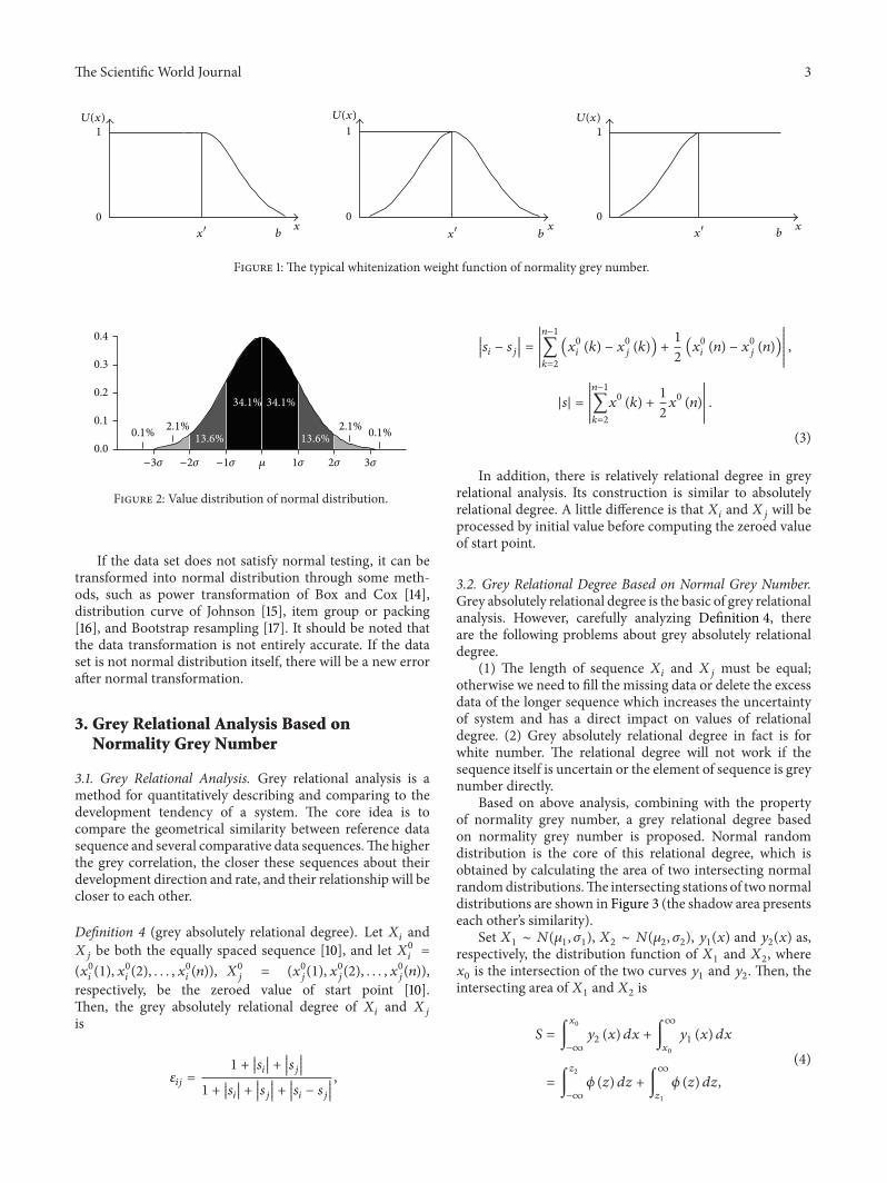