Embed Size (px)
Citation preview
Research ArticleSemisupervised Tangent Space Discriminant Analysis
Yang Zhou and Shiliang Sun
Shanghai Key Laboratory of Multidimensional Information Processing Department of Computer Science and TechnologyEast China Normal University 500 Dongchuan Road Shanghai 200241 China
Correspondence should be addressed to Shiliang Sun slsuncsecnueducn
Received 8 July 2014 Revised 5 November 2014 Accepted 14 November 2014
Academic Editor Xin Xu
Copyright copy 2015 Y Zhou and S Sun This is an open access article distributed under the Creative Commons Attribution Licensewhich permits unrestricted use distribution and reproduction in any medium provided the original work is properly cited
A novel semisupervised dimensionality reduction method named Semisupervised Tangent Space Discriminant Analysis (STSD) ispresented where we assume that data can be well characterized by a linear function on the underlying manifold For this purposea new regularizer using tangent spaces is developed which not only can capture the local manifold structure from both labeled andunlabeled data but also has the complementarity with the Laplacian regularizer Furthermore STSD has an analytic form of theglobal optimal solution which can be computed by solving a generalized eigenvalue problem To perform nonlinear dimensionalityreduction and process structured data a kernel extension of our method is also presented Experimental results on multiple real-world data sets demonstrate the effectiveness of the proposed method
1 Introduction
Dimensionality reduction is to find a low-dimensional rep-resentation of high-dimensional data while preserving datainformation as much as possible Processing data in the low-dimensional space can reduce computational cost and sup-press noises Provided that dimensionality reduction is per-formed appropriately the discovered low-dimensional rep-resentation of data will benefit subsequent tasks for exam-ple classification clustering and data visualization Clas-sical dimensionality reduction methods include supervisedapproaches like linear discriminant analysis (LDA) [1] andunsupervised ones such as principal component analysis(PCA) [2]
LDA is a supervised dimensionality reduction methodIt finds a subspace in which the data points from differentclasses are projected far away from each other while thedata points belonging to the same class are projected as closeas possible One merit of LDA is that LDA can extract thediscriminative information of data which is crucial for classi-fication Due to its effectiveness LDA is widely used in manyapplications for example bankruptcy prediction face recog-nition and data mining However LDA may get undesirableresults when the labeled examples used for learning are not
sufficient because the between-class scatter and the within-class scatter of data could be estimated inaccurately
PCA is a representative of unsupervised dimensionalityreduction methods It seeks a set of orthogonal projectiondirections along which the sum of the variances of data ismaximized PCA is a common data preprocessing techniqueto find a low-dimensional representation of high-dimen-sional data In order to meet the requirements of differentapplications many unsupervised dimensionality reductionmethods have been proposed such as Laplacian Eigen-maps [3] Hessian Eigenmaps [4] Locally Linear Embedding[5] Locality Preserving Projections [6] and Local TangentSpace Alignment [7] Although it is shown that unsupervisedapproaches work well in many applications they may not bethe best choices for some learning scenarios because theymayfail to capture the discriminative structure from data
Inmany real-world applications only limited labeled datacan be accessed while a large number of unlabeled data areavailable In this case it is reasonable to perform semisuper-vised learning which can utilize both labeled and unlabeleddata Recently several semisupervised dimensionality reduc-tion methods have been proposed for example Semisu-pervised Discriminant Analysis (SDA) [8] SemisupervisedDiscriminantAnalysis (SSDA)with path-based similarity [9]
Hindawi Publishing CorporationMathematical Problems in EngineeringVolume 2015 Article ID 706180 10 pageshttpdxdoiorg1011552015706180
2 Mathematical Problems in Engineering
and Semisupervised Local Fisher Discriminant Analysis(SELF) [10] SDA aims to find a transformation matrix fol-lowing the criterion of LDA while imposing a smoothnesspenalty on a graphwhich is built to exploit the local geometryof the underlying manifold Similarly SSDA also builds agraph for semisupervised learning However the graph isconstructed using a path-based similarity measure to capturethe global structure of data SELF combines the ideas of localLDA [11] and PCA so that it can integrate the informationbrought by both labeled and unlabeled data
Although all of these methods have their own advantagesin semisupervised learning the essential strategy of manyof them for utilizing unlabeled data relies on the Laplacianregularization In this paper we present a novel methodnamed Semisupervised Tangent SpaceDiscriminant Analysis(STSD) for semisupervised dimensionality reduction whichcan reflect the discriminant information and a specific man-ifold structure from both labeled and unlabeled data Unlikeadopting the Laplacian based regularizer we develop a newregularization term which can discover the linearity of thelocal manifold structure of data Specifically by introducingtangent spaces we represent the local geometry at each datapoint as a linear function and make the change of suchfunctions as smooth as possible This means that STSDappeals to a linear function on the manifold In additionthe objective function of STSD can be optimized analyticallythrough solving a generalized eigenvalue problem
2 Preliminaries
Consider a data set consisting of ℓ examples and labels(x119894 119910119894)ℓ
119894=1 where x
119894isin R119889 denotes a 119889-dimensional example
119910119894
isin 1 2 119862 denotes the class label correspondingto x119894 and 119862 is the total number of classes LDA seeks
a transformation t such that the between-class scatter ismaximized and the within-class scatter is minimized [1] Theobjective function of LDA can be written as
t(LDA) = arg maxt
t⊤119878119887t
t⊤119878119908t (1)
where ⊤ denotes the transpose of a matrix or a vector 119878119887is
the between-class scatter matrix and 119878119908is the within-class
scatter matrix The definitions of 119878119887and 119878119908are
119878119887=
119862
sum
119888=1
ℓ119888(120583119888minus 120583) (120583
119888minus 120583)⊤ (2)
119878119908=
119862
sum
119888=1
sum
119894|119910119894=119888
(x119894minus 120583119888) (x119894minus 120583119888)⊤ (3)
where ℓ119888is the number of examples from the 119888th class
120583 = (1ℓ)sumℓ
119894=1x119894is the mean of all the examples and 120583
119888=
(1ℓ119888) sum119894|119910119894=119888
x119894is the mean of the examples from class 119888
Define the total scatter matrix as
119878119905=
ℓ
sum
119894=1
(x119894minus 120583) (x
119894minus 120583)⊤ (4)
It is well known that 119878119905= 119878119887+ 119878119908[1] and (1) is equivalent to
t(LDA) = arg maxt
t⊤119878119887t
t⊤119878119905t (5)
The solution of (5) can be readily obtained by solving ageneralized eigenvalue problem 119878
119887t = 120582119878
119905t It should be
noted that the rank of the between-class scatter matrix 119878119887
is at most 119862 minus 1 and thus we can obtain at most 119862 minus 1
meaningful eigenvectors with respect to nonzero eigenvaluesThis implies that LDA can project data into a space whosedimensionality is at most 119862 minus 1
In practice we usually impose a regularizer on (5) toobtain amore stable solutionThen the optimization problembecomes
maxt
t⊤119878119887t
t⊤119878119905t + 120573119877 (t)
(6)
where 119877(t) denotes the imposed regularizer and 120573 is a trade-off parameter When we use the Tikhonov regularizer that is119877(t) = t⊤t the optimization problem is usually referred to asRegularized Discriminant Analysis (RDA) [12]
3 Semisupervised Tangent SpaceDiscriminant Analysis
As a supervised method LDA has no ability to extract infor-mation from unlabeled data Motivated by Tangent SpaceIntrinsic Manifold Regularization (TSIMR) [13] we developa novel regularizer to capture the manifold structure of bothlabeled andunlabeled dataUtilizing this regularizer the LDAmodel can be extended to a semisupervised one following theregularization frameworkThen we will first derive our novelregularizer for semisupervised learning and then presentour Semisupervised Tangent Space Discriminant Analysis(STSD) algorithm as well as its kernel extension
31The Regularizer for Semisupervised Dimensionality Reduc-tion TSIMR [13] is a regularizationmethod for unsuperviseddimensionality reduction which is intrinsic to data manifoldand favors a linear function on the manifold Inspired byTSIMR we employ tangent spaces to represent the localgeometry of data Suppose that the data are sampled froman 119898-dimensional smooth manifold M in a 119889-dimensionalspace LetTzM denote the tangent space attached to z wherez isin M is a fixed data point on the M Using the first-orderTaylor expansion at z any function119891 defined on themanifoldM can be expressed as
119891 (x) = 119891 (z) + w⊤z uz (x) + 119874 (x minus z2) (7)
where x isin R119889 is a 119889-dimensional data point and uz(x) =
119879⊤
z (xminusz) is an119898-dimensional tangent vector which gives the119898-dimensional representation of x in TzM 119879z is a 119889 times 119898
matrix formed by the orthonormal bases ofTzM which canbe estimated through local PCA that is performing standardPCA on the neighborhood of z wz is an 119898-dimensional
Mathematical Problems in Engineering 3
vector representing the directional derivative of 119891 at z withrespect to uz(x) on the manifoldM
Consider a transformation t isin R119889 which can map the 119889-dimensional data to a one-dimensional embeddingThen theembedding of x can be expressed as 119891(x) = t⊤x If there aretwo data points z and z1015840 that have a small Euclidean distanceby using the first-order Taylor expansion at z1015840 and z theembeddings 119891(z) and 119891(z1015840) can be represented as
119891 (z) = 119891 (z1015840) + w⊤z1015840uz1015840 (z) + 119874 (10038171003817100381710038171003817z minus z101584010038171003817100381710038171003817
2
) (8)
119891 (z1015840) = 119891 (z) + w⊤z uz (z1015840) + 119874(
10038171003817100381710038171003817z1015840 minus z10038171003817100381710038171003817
2
) (9)
Suppose that the data can be well characterized by a linearfunction on the underlyingmanifoldMThen the remaindersin (8) and (9) can be omitted
Substituting 119891(x) = t⊤x into (8) we have
t⊤z asymp t⊤z1015840 + w⊤z1015840119879⊤
z1015840 (z minus z1015840) (10)
Furthermore by substituting (9) into (8) we obtain
(119879z1015840wz1015840 minus 119879zwz)⊤(z minus z1015840) asymp 0 (11)
which naturally leads to
119879zwz asymp 119879z1015840wz1015840 (12)
Since 119879z is formed by the orthonormal bases of TzM itsatisfies119879⊤z 119879z = 119868
(119898times119898)for all z where 119868
(119898times119898)is an 119898-dimen-
sional identitymatrixWe canmultiply both sides of (12) with119879⊤
z then (12) becomes to
wz asymp 119879⊤
z 119879z1015840wz1015840 (13)
Armed with the above results we can formulate ourregularizer for semisupervised dimensionality reductionConsider data x
119894isin 119883 (119894 = 1 119899) sampled from a function
119891 along the manifold M Since every example x119894and its
neighbors should satisfy (10) and (13) it is reasonable toformulate a regularizer as follows
119877 (tw) =119899
sum
119894=1
sum
119895isinN(x119894)[ (t⊤ (x
119894minus x119895)
minus w⊤x119895119879⊤
x119895 (x119894 minus x119895))
2
+120574100381710038171003817100381710038171003817wx119894 minus 119879
⊤
x119894119879x119895wx119895100381710038171003817100381710038171003817
2
2
]
(14)
where w = (w⊤x1 w⊤
x2 w⊤
x119899)⊤ N(x
119894) denotes the set of
nearest neighbors of x119894 and 120574 is a trade-off parameter to
control the influences of (10) and (13)Relating data with a discrete weighted graph is a popular
choice and there are indeed a large family of graph basedstatistical andmachine learningmethods It also makes sensefor us to generalize the regularizer 119877(tw) in (14) using asymmetric weight matrix 119882 constructed from the above
data collection 119883 There are several manners to construct119882 One typical way is to build an adjacency graph byconnecting each data point to its 119896-nearest-neighbors withan edge and then weight every edge of the graph by a certainmeasure Generally if two data points x
119894and x
119895are ldquocloserdquo
the corresponding weight 119882119894119895is large whereas if they are
ldquofar awayrdquo then the119882119894119895is small For example the heat kernel
function is widely used to construct a weight matrix Theweight119882
119894119895is computed by
119882119894119895= exp(minus
10038171003817100381710038171003817x119894minus x119895
10038171003817100381710038171003817
2
1205902) (15)
if there is an edge connecting x119894with x
119895and 119882
119894119895= 0
otherwiseTherefore the generalization of the proposed regularizer
turns out to be
119877 (tw) =119899
sum
119894=1
119899
sum
119895=1
119882119894119895[ (t⊤ (x
119894minus x119895)
minus w⊤x119895119879⊤
x119895 (x119894 minus x119895))
2
+ 120574100381710038171003817100381710038171003817wx119894 minus 119879
⊤
x119894119879x119895wx119895100381710038171003817100381710038171003817
2
2
]
(16)
and 119882 is an 119899 times 119899 symmetric weight matrix reflecting thesimilarity of the data points It is clear that when the variationof the first-order Taylor expansion at every data point issmooth the value of 119877(tw) which measures the linearity ofthe function 119891 along the manifoldM will be small
The regularizer (16) can be reformulated as a canonicalmatrix quadratic form as follows
119877 (tw) = (tw)⊤
119878 (tw)
= (tw)⊤
(1198831198781119883⊤
1198831198782
119878⊤
2119883⊤
1198783
)(tw)
(17)
where 119883 = (x1 x
119899) is the data matrix and 119878 is a pos-
itive semidefinite matrix constructed by four blocks thatis 119883119878
1119883⊤ 119883119878
2 119878⊤2119883⊤ and 119878
3 This formulation will be
very useful in developing our algorithm Recall that thedimensionality of the directional derivative wx119894 (119894 = 1 119899)is119898Thereby the size of 119878 is (119889+119898119899)times(119889+119898119899) For simplicitywe omit the detailed derivation of 119878
It should be noted that besides the principle thataccorded with TSIMR the regularizer (16) can be explainedfrom another perspective Recently Lin et al [14] proposeda regularization method called Parallel Field Regularization(PFR) for semisupervised regression In spite of the differentlearning scenarios PFR shares the same spirit with TSIMRin essence Moreover when the bases of the tangent spaceTzM at any data point z are orthonormal PFR can beconverted to TSIMR It also provides a more theoretical butcomplex explanation for our regularizer from the vector fieldperspective
4 Mathematical Problems in Engineering
Input Labeled and unlabeled examples (x119894 119910119894) | x119894isin R119889 119910
119894isin
1 2 119862ℓ
119894=1 x119894| x119894isin R119889
119899
119894=ℓ+1
Trade-off parameters 120572 120573 120574 (120572 120573 120574 ge 0)Output 119889 times 119862 transformation matrix 119879Construct the adjacency graphCalculate the weight matrix119882for 119894 = 1 to 119899 doConstruct 119879x119894 using local PCA
end forCompute the eigenvectors f
1 f2 f
119862of (20) with respect to the non-zero
eigenvalues119879 = (t
1 t2 t
119862)
Algorithm 1 STSD
32 An Algorithm With the regularizer developed inSection 31 we can present our STSD algorithm Supposethe training data include ℓ labeled examples (x
119894 119910119894)ℓ
119894=1
belonging to 119862 classes and 119899 minus ℓ unlabeled examples x119894119899
119894=ℓ+1
where x119894
isin R119889 is a 119889-dimensional example and 119910119894
isin
1 2 119862 is the class label associated with the example x119894
Define f = (t⊤w⊤)⊤ and let 119878119887
= (119878119887 00 0 ) 119878119905 = (
119878119905 00 0 )
be two (119889 + 119898119899) times (119889 + 119898119899) augmented matrices extendedfrom the between-class scatter matrix 119878
119887and the total scatter
matrix 119878119905 Note that in the semisupervised learning scenario
discussed in this section the mean of all the samples in (2)and (4) should be the center of both the labeled and unlabeledexamples that is 120583 = (1119899)sum
119899
119894=1x119894 The objective function of
STSD can be written as follows
maxf
f⊤119878119887f
f⊤ (119878119905+ 120572119878) f
(18)
where 120572 is a trade-off parameter It is clear that f⊤119878119887f = t⊤119878
119887t
and f⊤119878119905f = t⊤119878
119905t Therefore STSD seeks an optimal f such
that the between-class scatter is maximized and the totalscatter as well as the regularizer 119877(tw) defined in (17) isminimized at the same time
The optimization of the objective function (18) can beachieved by solving a generalized eigenvalue problem
119878119887f = 120582 (119878
119905+ 120572119878) f (19)
whose solution can be easily given by the eigenvector withrespect to the maximal eigenvalue Note that since the meanu is the center of both labeled and unlabeled examples therank of 119878
119887is119862 It implies that there are at most119862 eigenvectors
with respect to the nonzero eigenvalues Therefore given theoptimal eigenvectors f
1 f
119862 we can form a transformation
matrix sized 119889 times 119862 as 119879 = (t1 t
119862) and then the 119862-
dimensional embedding b of an example x can be computedthrough b = 119879
⊤xIn many applications especially when the dimensionality
of data is high while the data size is small the matrix 119878119905+ 120572119878
in (19) may be singular This singularity problem may lead
to an unstable solution and deteriorate the performance ofSTSD Fortunately there are many approaches to deal withthe singularity problem In this paper we use the Tikhonovregularization because of its simplicity and wide applicabilityFinally the generalized eigenvalue problem (19) turns out tobe
119878119887f = 120582 (119878
119905+ 120572119878 + 120573119868) f (20)
where 119868 is the identity matrix and 120573 ge 0 Algorithm 1 givesthe pseudocode for STSD
The main computational cost of STSD lies in buildingtangent spaces for 119899 data points and solving the generalizedeigenvalue problem (20) The naive implementation for ouralgorithm has a runtime of 119874((1198892119898 + 119898
2119889) times 119899) for the
construction of tangent spaces and 119874((119889 + 119898119899)3) for the
generalized eigenvalue decomposition This suggests thatSTSD might be a time-consuming method
However given a neighborhood size 119896 there are only 119896+1examples as the inputs of local PCA Then we can obtain atmost 119896 + 1 meaningful orthonormal bases to construct eachtangent space which implies that the dimensionality119898 of thedirectional derivative wx119894 (119894 = 1 119899) is always less than119896+1 In practice 119896 is usually small to ensure the localityThismakes sure that 119898 is actually a small constant Furthermorerecall that the number of eigenvectorswith respect to nonzeroeigenvalues is equal to the number of classes 119862 Using thetechnique of sparse generalized eigenvalue decompositionthe corresponding computational cost is reduced to 119874(119862
2times
(119889 + 119898119899))In summary the overall runtime of STSD is 119874((1198892119898 +
1198982119889) times 119899 + 119862
2times (119889 + 119898119899)) Since 119898 and 119862 are always small
STSD actually has an acceptable computational cost
33 Kernel STSD Essentially STSD is a linear dimensionalityreduction method which can not be used for nonlineardimensionality reduction or processing structured data suchas graphs trees or other types of structured inputs To handlethis problem we extend STSD to a Reproducing KernelHilbert Space (RKHS)
Mathematical Problems in Engineering 5
Suppose examples x119894isin X (119894 = 1 119899) where X is
an input domain Consider a feature space F induced by anonlinear mapping 120601 X rarr F We can construct an RKHS119867K by defining a kernel function K(sdot sdot) using the innerproduct operation ⟨sdot sdot⟩ such that K(x y) = ⟨120601(x) 120601(y)⟩Let Φ
119897= (120601(x
1) 120601(x
ℓ)) Φ119906
= (120601(xℓ+1
) 120601(x119899)) be
the labeled and unlabeled data matrix in the feature spaceF respectively Then the total data matrix can be written asΦ = (Φ
119897 Φ119906)
Let 120601(120583) be the mean of all the examples inF and defineΨ = (120601(120583
1) 120601(120583
119862)) which is constituted by the mean
vectors of each class in F Suppose that 120601(120583) = 0 (it canbe easily achieved by centering the data in the feature space)and the labeled examples inΦ
119897are ordered according to their
labels Then the between-class scatter matrix 119878120601119887and the total
scatter matrix 119878120601
119905in F can be written as 119878120601
119887= Ψ119872Ψ
⊤ 119878120601119905=
Φ119868Φ⊤ where 119872 is a 119862 times 119862 diagonal matrix whose (119888 119888)th
element is the number of the examples belonging to class 119888and 119868 = (
119868ℓtimesℓ 00 0 ) is a 119899 times 119899 matrix where 119868
ℓtimesℓis the identity
matrix sized ℓ times ℓRecall that STSD aims to find a set of transformations
to map data into a low-dimensional space Given examplesx1 x
119899 one can use the orthogonal projection to decom-
pose any transformation t isin 119867K into a sum of two functionsone lying in the 119904119901119886119899120601(x
1) 120601(x
119899) and the other one
lying in the orthogonal complementary space Thereforethere exist a set of coefficients 120572
119894(119894 = 1 2 119899) satisfying
t =119899
sum
119894=1
120572119894120601 (x119894) + k = Φ120572 + k (21)
where 120572 = (1205721 1205722 120572
119899)⊤ and ⟨k 120601(x
119894)⟩ = 0 for all 119894 Note
that although we set f = (t⊤w⊤)⊤ and optimize t and wtogether there is no need to reparametrize w like t What weneed is to estimate tangent spaces inF through local KernelPCA [15]
Let 119879120601x119894 be the matrix formed by the orthonormal bases ofthe tangent space attached to 120601(x
119894) Substitute (21) into (17)
and replace 119879x119894 with 119879120601
x119894 (119894 = 1 2 119899) We can reformulatethe regularizer (17) as follows
119877 (120572w) = 120572⊤Φ⊤Φ1198781Φ⊤Φ120572 + w⊤119878
3w
+ 120572⊤Φ⊤Φ1198782w + w⊤119878⊤
2Φ⊤Φ120572
= 120572⊤1198701198781119870120572 + w⊤119878
3w
+ 120572⊤1198701198782w + w⊤119878⊤
2119870120572
(22)
where 119870 is a kernel matrix with 119870119894119895= K(x
119894 x119895) With this
formulation Kernel STSD can be converted to a generalizedeigenvalue problem as follows
119878120601
119887120593 = 120582 (119878
120601
119905+ 120572119878120601)120593 (23)
where we have defined 120593 = (120572⊤w⊤)⊤ The definitions of 119878120601
119887
119878120601
119905 and 119878
120601 are given as follows
119878120601
119887= (
Φ⊤119878120601
119887Φ 0
0 0) = (Φ⊤Ψ119872Ψ
⊤Φ 0
0 0)
119878120601
119905= (
Φ⊤119878120601
119905Φ 0
0 0) = (119870119868119870 00 0)
119878120601= (
1198701198781119870 119870119878
2
119878⊤
2119870 119878
3
)
(24)
It should be noted that every term of k vanishes from theformulation of Kernel STSD because ⟨k 120601(x
119894)⟩ = 0 for all 119894
SinceΨ⊤Φ can be computed through the kernelmatrix119870 thesolution of Kernel STSD can be obtained without knowingthe explicit form of the mapping 120601
Given the eigenvectors 1205931 120593
119862with respect to the
nonzero eigenvalues of (23) the resulting transformationmatrix can be written as Γ = (120572
1 120572
119862) Then the embed-
ding b of an original example x can be computed as
b = Γ⊤Φ⊤120601 (x) = Γ
⊤(K (x
1 x) K (x
119899 x))⊤ (25)
4 Experiments
41 Toy Data In order to illustrate the behavior of STSDwe first perform STSD on a toy data set (two moons)compared with PCA and LDA The toy data set contains 100data points and is used under different label configurationsSpecifically 6 10 50 and 80 data points are randomly labeledrespectively and the rest are unlabeled where PCA is trainedby all the data points without labels LDA is trained bylabeled data only and STSD is trained by both the labeledand unlabeled data In Figure 1 we show the one-dimensionalembedding spaces found by different methods (onto whichdata points will be projected) As can be seen in Figure 1(a)although LDA is able to find an optimum projection wherethe within-class scatter is minimized while the between-class separability is maximized it can hardly find a goodprojection when the labeled data are scarce In addition PCAalso finds a bad solution since it has no ability to utilize thediscriminant information from class labels On the contrarySTSD which can utilize both the labeled and unlabeled datafinds a desirable projection onto which data from differentclasses have the minimal overlap As the number of labeleddata increases we can find that the solutions of PCA andSTSD do not change while the projections found by PCA aregradually close to those of STSD In Figure 1(d) the solutionsof LDA and STSD are almost identical which means that byutilizing both labeled and unlabeled data STSD can obtainthe optimum solutions even when only a few data points arelabeled This demonstrates the usefulness and advantage ofSTSD in the semisupervised scenario
42 Real-World Data In this section we evaluate STSD withreal-world data sets Specifically we first perform dimension-ality reduction to map all examples into a subspace and thencarry out classification using the nearest neighbor classifier
6 Mathematical Problems in Engineering
0 1 2 3
0
1
2
3
minus3
minus3
minus2
minus2
minus1
minus1
(a) 6 labeled
0
1
2
3
minus3
minus2
minus1
0 1 2 3minus3 minus2 minus1
(b) 10 labeled
STSDLDAPCA
0
1
2
3
minus3
minus2
minus1
0 1 2 3minus3 minus2 minus1
(c) 50 labeled
STSDLDAPCA
0
1
2
3
minus3
minus2
minus1
0 1 2 3minus3 minus2 minus1
(d) 80 labeled
Figure 1 Illustrative examples of STSD LDA and PCA on the two-moon data set under different label configurationsThe circles and squaresdenote the data points in positive and negative classes and the filled or unfilled symbols denote the labeled or unlabeled data respectively
(1-NN) in the subspace This measurement for evaluatingsemisupervised dimensionality reduction methods is widelyused in literature such as [8ndash10 16] For each data set werandomly split out 80 of the data as the training set andthe rest as the test set In the training set a certain numberof data are randomly labeled while the rest of the data areunlabeled Moreover every experimental result is obtainedfrom the average over 20 splits
In our experiments we compare STSD with multipledimensionality reduction methods including PCA LDASELF and SDA where LDA is performed only on the labeleddata while PCA SELF SDA and STSD are performed onboth the labeled and unlabeled data In addition we alsocompare our method with the baseline method which justemploys the 1-NN classifier with the labeled data in theoriginal space Since the performances of PCA and SELF
Mathematical Problems in Engineering 7
Table 1 Mean values and standard deviations of the unlabeled error rates () with different label configurations on the face data sets
Method Yale 3 Yale 4 ORL 2 ORL 3Baseline 4950 plusmn 486 4393 plusmn 471 3031 plusmn 311 2113 plusmn 229PCA 4767 plusmn 440 4260 plusmn 505 2923 plusmn 256 2030 plusmn 222LDA 3256 plusmn 385 2560 plusmn 298 1717 plusmn 323 805 plusmn 251SELF 5422 plusmn 388 5207 plusmn 467 4879 plusmn 439 3748 plusmn 281SDA 3233 plusmn 411 2593 plusmn 322 1667 plusmn 336 785 plusmn 248STSD 3228 plusmn 409 2527 plusmn 361 1600 plusmn 303 773 plusmn 230
Table 2 Mean values and standard deviations of the test error rates () with different label configurations on the face data sets
Method Yale 3 Yale 4 ORL 2 ORL 3Baseline 4617 plusmn 767 4667 plusmn 865 2994 plusmn 366 1919 plusmn 350PCA 4067 plusmn 806 4200 plusmn 729 2806 plusmn 392 1813 plusmn 371LDA 3233 plusmn 831 2617 plusmn 774 1656 plusmn 397 913 plusmn 363SELF 5000 plusmn 649 4933 plusmn 828 4788 plusmn 482 3556 plusmn 352SDA 3200 plusmn 840 2617 plusmn 767 1613 plusmn 405 900 plusmn 333STSD 3183 plusmn 841 2533 plusmn 854 1569 plusmn 368 900 plusmn 316
depend on the dimensionality of the embedding subspacediscovered by eachmethod we show the best results for them
For the graph based methods including SELF SDA andSTSD the number of nearest neighbors for constructingadjacency graphs is determined by fourfold cross-validationThe parameters 120572 and 120574 for STSD are selected throughfourfold cross-validation while the Tikhonov regularizationparameter 120573 is fixed to 10
minus1 In addition the parametersinvolved in SELF and SDA are also selected through fourfoldcross-validation We use the heat kernel function (15) toconstruct the weight matrix and the kernel parameter 1205902 isfixed as119889av unless otherwise specifiedwhere119889av is the averageof the squared distances between all data points and theirnearest neighbors
Two types of data sets under different label configurationsare used to conduct our experiments One type of data sets isthe face images which consist of high-dimensional imagesand the other one is the UCI data sets constituted by low-dimensional data For the convenience of description wename each configuration of experiments as ldquoData Setrdquo +ldquoLabeled Data Sizerdquo For example for the experiments withthe face images ldquoYale 3rdquo means the experiment is performedon the Yale data set with 3 labeled data per class Analogouslyfor the experiments with the UCI data sets ldquoBCWD 20rdquomeans the experiment is performed on the Breast CancerWisconsin (Diagnostic) data set with a total of 20 labeledexamples from all classes
421 Face Images It is well known that high-dimensionaldata such as images and texts are supposed to live on ornear a low-dimensional manifold In this section we testour algorithm with the Yale and ORL face data sets whichare deemed to satisfy this manifold assumption The Yaledata set contains 165 images of 15 individuals and thereare 11 images per subject The images have different facial
expressions illuminations and facial details (with or withoutglass) The ORL data set contains 400 images of 40 distinctsubjects under varying expressions and illuminations In ourexperiments every face image is cropped to consist of 32times32pixels with 256 grey levels per pixel Furthermore for the Yaledata set we set the parameter 1205902 of the heat kernel to 01119889avWe report the error rates on both the unlabeled training dataand test data Tables 1 and 2 show that STSD is always betterthan or at least comparable with other counterparts in allthe cases which demonstrates that STSD can well exploit themanifold structure for dimensionality reduction Notice thatSELF gets inferior results We conjecture that this is becauseit has no ability to capture the underlyingmanifold structuresof the data
422 UCI Data Sets In this set of experiments we usethree UCI data sets [17] including Breast Cancer Wiscon-sin (Diagnostic) Climate Model Simulation Crashes andCardiotocography which may not well satisfy the manifoldassumption For simplicity we abbreviate these data sets asBCWD CMSC and CTG respectively BCWD consists of569 data points from two classes in R30 CMSC consists of540 data points from two classes inR18 CTG consists of 2126data points from ten classes in R23
From the results reported in Tables 3 and 4 it can beseen that when the labeled data are scarce the performanceof LDA is even worse than the baseline method due tothe inaccurate estimation of the scatter matrices HoweverSTSD achieves the best or comparable results among allother methods in all configurations expect for the test errorrate in BCWD 10 Although STSD adopts a relatively strongmanifold assumption it still has sufficient flexibility to handlegeneral data which may not live on a low-dimensionalmanifold
8 Mathematical Problems in Engineering
Table 3 Mean values and standard deviations of the unlabeled error rates () with different label configurations on the UCI data sets
Method BCWD 10 BCWD 30 CMSC 10 CMSC 30 CTG 20 CTG 160Baseline 1190 plusmn 404 1022 plusmn 321 1439 plusmn 640 1405 plusmn 190 6371 plusmn 373 4791 plusmn 173PCA 1187 plusmn 401 1021 plusmn 327 1186 plusmn 251 1343 plusmn 240 6374 plusmn 375 4789 plusmn 166LDA 2034 plusmn 876 961 plusmn 276 1318 plusmn 449 1421 plusmn 328 6728 plusmn 632 4160 plusmn 265SELF 1343 plusmn 363 141 plusmn 420 1006 plusmn 330 1188 plusmn 253 6700 plusmn 450 4409 plusmn 266SDA 1010 plusmn 326 712 plusmn 217 906 plusmn 097 871 plusmn 078 5827 plusmn 501 4191 plusmn 217STSD 1007 plusmn 346 699 plusmn 173 898 plusmn 104 860 plusmn 058 5811 plusmn 478 4088 plusmn 215
Table 4 Mean values and standard deviations of the test error rates () with different label configurations on the UCI data sets
Method BCWD 10 BCWD 30 CMSC 10 CMSC 30 CTG 20 CTG 160Baseline 1275 plusmn 656 1065 plusmn 420 1463 plusmn 848 1281 plusmn 437 6415 plusmn 474 4876 plusmn 244PCA 1275 plusmn 656 1050 plusmn 416 875 plusmn 190 913 plusmn 266 6407 plusmn 476 4866 plusmn 241LDA 2060 plusmn 1034 1085 plusmn 506 1319 plusmn 566 1513 plusmn 535 6747 plusmn 727 4195 plusmn 343SELF 1465 plusmn 688 1370 plusmn 437 906 plusmn 266 869 plusmn 184 6702 plusmn 506 4334 plusmn 281SDA 975 plusmn 360 875 plusmn 309 869 plusmn 315 806 plusmn 170 5872 plusmn 426 4167 plusmn 311STSD 1015 plusmn 455 850 plusmn 319 863 plusmn 259 806 plusmn 154 5862 plusmn 411 4155 plusmn 331
Notice that the error rates of several dimensionalityreduction methods over the CMSC data set do not improvewith the increasing size of labeled data The reason may bethat the data in the CMSC data set contain some irrelevantfeatures as reflected by the original data description [18]which leads to the unexpected results Nevertheless SDA andSTSDachievemore reasonable results due to their capabilitiesto extract information from both labeled and unlabeled data
It should be noted that overall the experiments areconducted with 5 data sets and in terms of the results of allthe data sets STSD is likely to beat other methods account fora sign-testrsquos 119875 value of 0031 which is statistically significantThis also demonstrates that STSD is better than the relatedmethods
43 Connection with the Laplacian Regularization Essen-tially both STSD and SDA are regularized LDA methodswith specific regularizers STSD imposes the regularizer (16)which prefers a linear function along themanifold while SDAemploys the Laplacian regularizer to penalize the functiondifferences among ldquosimilarrdquo examples Now consider a regu-larized LDA method using both of these regularizers namedSTSLap whose objective function can be written as follows
maxtw
t⊤119878119887t
t⊤119878119905t + 120572119877Lap (t) + 120573119877STS (tw)
(26)
where119877Lap(t) = t⊤119871t is the Laplacian regularizer used in SDAwith 119871 being the Laplacian matrix [19] and 119877STS(tw) is theregularizer used in STSDwhich is defined as (16)Theparam-eters 120572 and 120573 are used to control the trade-off between theinfluences of 119877Lap(t) and 119877STS(tw) Similar to STSD STSLapcan also be converted to a generalized eigenvalue problemwhich can be easily solved through eigenvalue decomposi-tion
Although the previous experiments have shown thatSTSD gets better results than SDA in most situations SDAcan achieve similar results with STSD in some configurationsHowever this does not mean that STSD and SDA are similaror in other words 119877STS(tw) and 119877Lap(t) have similar behav-ior In fact the two regularizers seem to complement eachother To demonstrate this complementarity we compareSTSLap with SDA and STSD under a medium-sized labelconfiguration over all the data sets used in the previousexperiments Specifically the experiments are performedon BCWD 30 CMSC 30 CTG 160 Yale 3 and ORL 2For each data set the neighborhood size used to constructthe adjacency graph is set to be the one supported by theexperimental results with both SDA and STSD in Sections421 and 422 This means that all the methods comparedin this section utilize the same graph to regularize the LDAmodel for each data set The parameters 120572 120573 in (26) and 120574 in119877STS(tw) are selected through fourfold cross-validation
Note that given a graph the performance of STSLap canbe at least ideally identical to SDA or STSD because STSLapdegenerates to SDA or STSDwhen the parameter 120572 or 120573 is setto zero However if STSLap achieves better results than bothSDA and STSD we can deem that 119877Lap(t) and 119877STS(tw) arecomplementary
Tables 5 and 6 show that the performance of STSLapis better than both SDA and STSD in most of the casesMoreover although it is not shown in the tables the trade-off parameters 120572 and 120573 are scarcely set to be zero bycross-validation This means that STSLap always utilizes theinformation discovered from both 119877Lap(t) and 119877STS(tw) Inconclusion the proposed regularizer 119877STS(tw) can capturethemanifold structure of data which can not be discovered byLaplacian regularizerThis implies that these two regularizersare complementary to each other and we could use themtogether to yield probably better results in practice It should
Mathematical Problems in Engineering 9
Table 5 Mean values and standard deviations of the unlabeled error rates () with medium-sized labeled data on different data sets
Method BCWD 30 CMSC 30 CTG 160 Yale 3 ORL 2SDA 688 plusmn 253 960 plusmn 227 4197 plusmn 272 3239 plusmn 598 2081 plusmn 276STSD 696 plusmn 245 940 plusmn 230 4347 plusmn 283 3256 plusmn 667 1648 plusmn 214STSLap 707 plusmn 246 960 plusmn 224 4157 plusmn 266 3339 plusmn 701 1642 plusmn 207
Table 6 Mean values and standard deviations of the test error rates () with medium-sized labeled data on different data sets
Method BCWD 30 CMSC 30 CTG 160 Yale 3 ORL 2SDA 690 plusmn 286 956 plusmn 328 4185 plusmn 323 3333 plusmn 592 2063 plusmn 598STSD 670 plusmn 281 944 plusmn 345 4247 plusmn 357 3300 plusmn 620 1481 plusmn 420STSLap 645 plusmn 274 938 plusmn 313 4118 plusmn 354 3283 plusmn 624 1444 plusmn 428
be noted that our aim is not to compare STSD with SDA inthis set of experiments and we can not make any conclusionabout whether or not STSD is better than SDA from Tables5 and 6 because the neighbourhood size for each data set isfixed
5 Discussion
51 Related Work STSD is a semisupervised dimensionalityreduction method under a certain manifold assumptionMore specifically we assume that the distribution of data canbe well approximated by a linear function on the underly-ing manifold One related method named SDA [8] adoptsanother manifold assumption It simply assumes that themapping function should be as smooth as possible on a givengraphThis strategy is well known as the Laplacian regulariza-tionwhich is widely employed in the semisupervised learningscenario However STSD follows a different principle toregularize the mapping function which not only providesan alternative strategy for semisupervised dimensionalityreduction but also attains the complementarity with theclassic Laplacian regularization SELF [10] is another relatedapproach which is a hybrid method of local LDA [11] andPCA Despite its simplicity SELF can only discover the linearstructure of data whereas our method is able to capture thenonlinear intrinsic manifold structure
Rather than constructing an appropriate regularizer ona given graph SSDA [9] and semisupervised dimensionalityreduction (SSDR) [16] focus on building a good graph andthen perform the Laplacian-style regularization on thisgraph SSDA regularizes LDA on a graph constructed by apath-based similarity measure The advantage of SSDA is itsrobustness against outliers because SSDA aims to preservethe global manifold information SSDR constructs a graphaccording to the so-called must-link and cannot-link pair-wise constraints which gives a natural way to incorporateprior knowledge into the semisupervised dimensionalityreduction However this prior knowledge is not alwaysavailable in practice In contrast to SSDA and SSDR ourmethod is flexible enough to perform regularization on anygraph and free from the necessity of extra prior knowledge Infact the advantage of SSDA or SSDR can be easily inherited
through performing STSD with the graph constructed bycorresponding method (SSDA or SSDR) which is anotherimportant merit of STSD
52 Further Improvements For the manifold related learningproblem considered in STSD the estimation of bases fortangent spaces is an important step In this paper we use localPCA with fixed neighborhood size to calculate the tangentspaces and the neighborhood size is set to be same as theone used to construct the adjacency graph This is certainlynot the optimal choice since manifolds can have varyingcurvatures and data could be nonuniformly sampled Notethat the neighborhood size can determine the evolution ofcalculated tangent spaces along the manifold When a smallneighborhood size 119896 is used there are at most 119896 + 1 examplesfor the inputs of local PCA However when we need toestimate a set of tangent spaces which have relative highdimensionality 119898 (119898 gt 119896 + 1) it is almost impossible to getaccurate estimates of the tangent spaces because there are atmost 119896+1meaningful orthonormal bases obtained from localPCA Moreover noises can damage the manifold assumptionas well to a certain extent All these factors explain thenecessity for using different neighborhood sizes and morerobust subspace estimation methods
In our method each example in the data matrix canbe treated as an anchor point where local PCA is used tocalculate the tangent space The number of parameters thatshould be estimated in our method basically grows linearlywith respect to the number of anchor points Therefore inorder to reduce the parameters to be estimated one possibleapproach is to reduce the anchor points where only ldquokeyrdquoexamples are kept as the anchor points This will be a kind ofresearch for data set sparsification People can make differentcriteria to decide whether or not an example should beregarded as the ldquokeyrdquo one
The research of anchor point reduction is especiallyuseful when training data are large-scale For large-scale dataanchor point reduction can be promising to speed up thetraining process In addition data can exhibit different man-ifold dimensions at different regions especially for complexdataTherefore adaptively determining the dimensionality at
10 Mathematical Problems in Engineering
different anchor points is also an important refinement of thecurrent approach
6 Conclusion
In this paper we have proposed a novel semisuperviseddimensionality reduction method named SemisupervisedTangent Space Discriminant Analysis (STSD) which canextract the discriminant information as well as the manifoldstructure from both labeled and unlabeled data where alinear function assumption on the manifold is exploitedLocal PCA is involved as an important step to estimatetangent spaces and certain relationships between adjacenttangent spaces are derived to reflect the adopted modelassumptionThe optimization of STSD is readily achieved bythe eigenvalue decomposition
Experimental results on multiple real-world data setsincluding the comparisons with related works have shownthe effectiveness of the proposed method Furthermore thecomplementarity between our method and the Laplacianregularization has also been verified Future work directionsinclude finding more accurate methods for tangent spaceestimation and extending our method to different learningscenarios such as multiview learning and transfer learning
Conflict of Interests
The authors declare that there is no conflict of interestsregarding the publication of this paper
Acknowledgments
This work is supported by the National Natural ScienceFoundation of China under Project 61370175 and ShanghaiKnowledge Service Platform Project (no ZF1213)
References
[1] K Fukunaga Introduction to Statistical Pattern RecognitionAcademic Press 2nd edition 1990
[2] I T Jolliffe Principal Component Analysis Springer New YorkNY USA 1986
[3] M Belkin and P Niyogi ldquoLaplacian eigenmaps for dimension-ality reduction and data representationrdquo Neural Computationvol 15 no 6 pp 1373ndash1396 2003
[4] D L Donoho andCGrimes ldquoHessian eigenmaps locally linearembedding techniques for high-dimensional datardquo Proceedingsof the National Academy of Sciences of the United States ofAmerica vol 100 no 10 pp 5591ndash5596 2003
[5] S T Roweis and L K Saul ldquoNonlinear dimensionality reduc-tion by locally linear embeddingrdquo Science vol 290 no 5500pp 2323ndash2326 2000
[6] X He and P Niyogi ldquoLocality preserving projectionsrdquo inAdvances in Neural Information Processing Systems S ThrunL Saul and B Scholkopf Eds vol 18 pp 1ndash8 MIT PressCambridge Mass USA 2004
[7] Z Zhang and H Zha ldquoPrincipal manifolds and nonlineardimensionality reduction via tangent space alignmentrdquo SIAMJournal on Scientific Computing vol 26 no 1 pp 313ndash338 2004
[8] D Cai X He and J Han ldquoSemi-supervised discriminant anal-ysisrdquo in Proceedings of the 11th IEEE International Conferenceon Computer Vision (ICCV rsquo07) pp 1ndash7 Rio de Janeiro BrazilOctober 2007
[9] Y Zhang andD-Y Yeung ldquoSemi-supervised discriminant anal-ysis using robust path-based similarityrdquo in Proceedings of theIEEE Conference on Computer Vision and Pattern Recognition(CVPR rsquo08) pp 1ndash8 Anchorage Alaska USA June 2008
[10] M Sugiyama T Ide S Nakajima and J Sese ldquoSemi-supervisedlocal Fisher discriminant analysis for dimensionality reduc-tionrdquoMachine Learning vol 78 no 1-2 pp 35ndash61 2010
[11] M Sugiyama ldquoDimensionality reduction ofmultimodal labeleddata by local fisher discriminant analysisrdquo The Journal ofMachine Learning Research vol 8 pp 1027ndash1061 2007
[12] J H Friedman ldquoRegularized discriminant analysisrdquo Journal oftheAmerican Statistical Association vol 84 no 405 pp 165ndash1751989
[13] S Sun ldquoTangent space intrinsicmanifold regularization for datarepresentationrdquo in Proceedings of the IEEE China Summit andInternational Conference on Signal and Information Processing(ChinaSIP rsquo13) pp 179ndash183 Beijing China July 2013
[14] B Lin C Zhang and X He ldquoSemi-supervised regression viaparallel field regularizationrdquo in Advances in Neural InformationProcessing Systems J Shawe-Taylor R S Zemel P Bartlett F CN Pereira and K QWeinberger Eds vol 24 pp 433ndash441TheMIT Press Cambridge Mass USA 2011
[15] B Scholkopf A Smola and K-R Muller ldquoNonlinear compo-nent analysis as a kernel eigenvalue problemrdquoNeural Computa-tion vol 10 no 5 pp 1299ndash1319 1998
[16] D Zhang Z Zhou and S Chen ldquoSemi-supervised dimension-ality reductionrdquo in Proceedings of the 7th SIAM InternationalConference on Data Mining pp 629ndash634 April 2007
[17] K Bache and M Lichman UCI machine learning repository2013 httparchiveicsucieduml
[18] D D Lucas R Klein J Tannahill et al ldquoFailure analysisof parameter-induced simulation crashes in climate modelsrdquoGeoscientific Model Development Discussions vol 6 no 1 pp585ndash623 2013
[19] F R K Chung Spectral GraphTheory AmericanMathematicalSociety Providence RI USA 1997
Submit your manuscripts athttpwwwhindawicom
Hindawi Publishing Corporationhttpwwwhindawicom Volume 2014
MathematicsJournal of
Hindawi Publishing Corporationhttpwwwhindawicom Volume 2014
Mathematical Problems in Engineering
Hindawi Publishing Corporationhttpwwwhindawicom
Differential EquationsInternational Journal of
Volume 2014
Applied MathematicsJournal of
Hindawi Publishing Corporationhttpwwwhindawicom Volume 2014
Probability and StatisticsHindawi Publishing Corporationhttpwwwhindawicom Volume 2014
Journal of
Hindawi Publishing Corporationhttpwwwhindawicom Volume 2014
Mathematical PhysicsAdvances in
Complex AnalysisJournal of
Hindawi Publishing Corporationhttpwwwhindawicom Volume 2014
OptimizationJournal of
Hindawi Publishing Corporationhttpwwwhindawicom Volume 2014
CombinatoricsHindawi Publishing Corporationhttpwwwhindawicom Volume 2014
International Journal of
Hindawi Publishing Corporationhttpwwwhindawicom Volume 2014
Operations ResearchAdvances in
Journal of
Hindawi Publishing Corporationhttpwwwhindawicom Volume 2014
Function Spaces
Abstract and Applied AnalysisHindawi Publishing Corporationhttpwwwhindawicom Volume 2014
International Journal of Mathematics and Mathematical Sciences
Hindawi Publishing Corporationhttpwwwhindawicom Volume 2014
The Scientific World JournalHindawi Publishing Corporation httpwwwhindawicom Volume 2014
Hindawi Publishing Corporationhttpwwwhindawicom Volume 2014
Algebra
Discrete Dynamics in Nature and Society
Hindawi Publishing Corporationhttpwwwhindawicom Volume 2014
Hindawi Publishing Corporationhttpwwwhindawicom Volume 2014
Decision SciencesAdvances in
Discrete MathematicsJournal of
Hindawi Publishing Corporationhttpwwwhindawicom
Volume 2014 Hindawi Publishing Corporationhttpwwwhindawicom Volume 2014
Stochastic AnalysisInternational Journal of
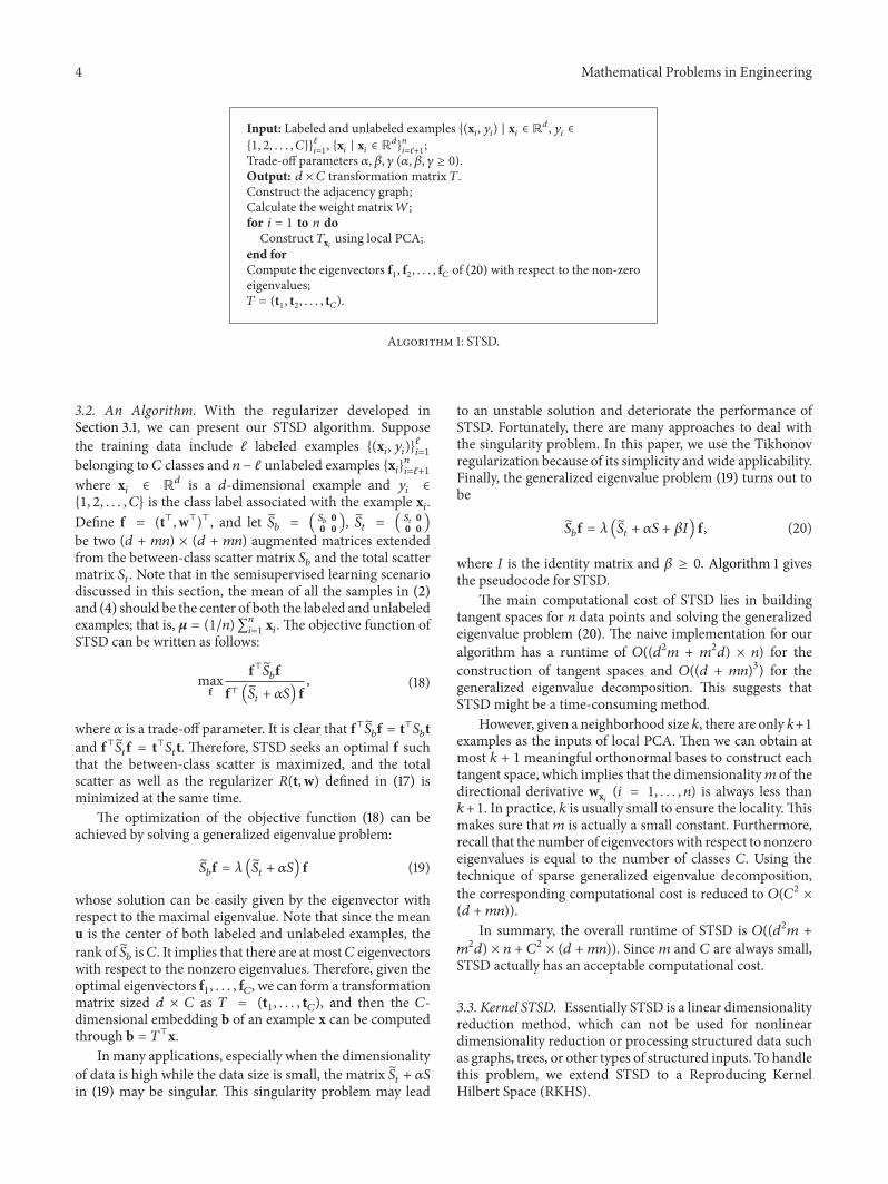
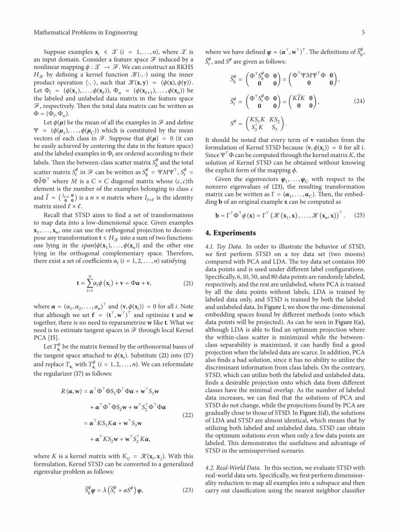
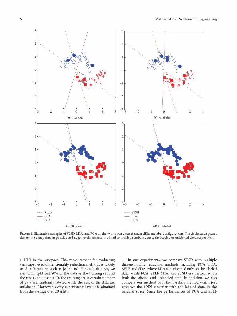
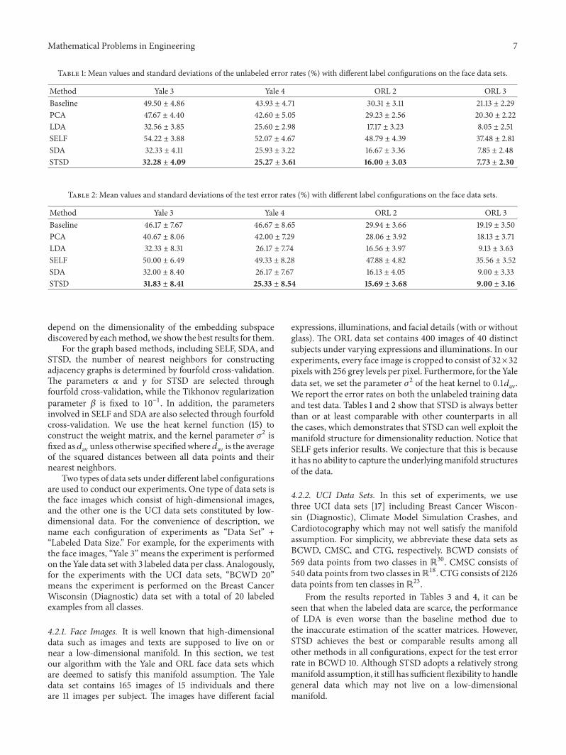
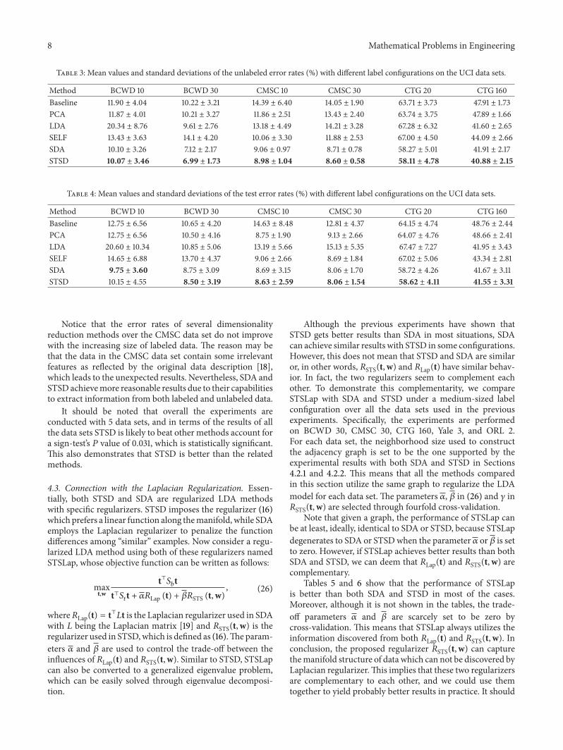
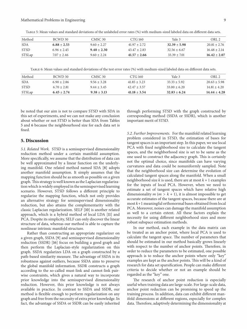