Embed Size (px)
Citation preview
Research ArticleSolution of Contact Problems for Nonlinear GaoBeam and Obstacle
J Machalovaacute and H Netuka
Faculty of Science Palacky University in Olomouc 17 listopadu 119212 771 46 Olomouc Czech Republic
Correspondence should be addressed to J Machalova jitkamachalovaupolcz
Received 21 May 2015 Revised 24 July 2015 Accepted 14 August 2015
Academic Editor Hui-Shen Shen
Copyright copy 2015 J Machalova and H NetukaThis is an open access article distributed under the Creative Commons AttributionLicense which permits unrestricted use distribution and reproduction in any medium provided the original work is properlycited
Contact problem for a large deformed beam with an elastic obstacle is formulated analyzed and numerically solved The beammodel is governed by a nonlinear fourth-order differential equation developed by Gao while the obstacle is considered as theelastic foundation of Winklerrsquos type in some distance under the beam The problem is static without a friction and modeled eitherusing Signorini conditions or by means of normal compliance contact conditions The problems are then reformulated as optimalcontrol problems which is useful both for theoretical aspects and for solution methods Discretization is based on using the mixedfinite element method with independent discretization and interpolations for foundation and beam elements Numerical examplesdemonstrate usefulness of the presented solution method Results for the nonlinear Gao beam are compared with results for theclassical Euler-Bernoulli beam model
1 Introduction
Contact problems belong to the most important industrialapplications and contact problems for beams have their ownsignificant position among them The Euler-Bernoulli beamis the most popular model used in engineering applicationsThis model is linear and its validity is limited only to relativesmall deflections If we suppose large deformations we haveto switch the mathematical model to a nonlinear one One ofthe best nonlinear beammodels was developed by Gao in [1]
In this paper we are going to deal with a beam and anelastic obstaclewhich are in possible contact For conveniencewe start our considerations with the classical Euler-Bernoullibeam model and the Winkler foundation Nowadays it iswell known that the contact of the elastic bodies is usuallymodeled using the Signorini conditions and followed byvariational inequalities (see eg [2 3])
But this approach is necessary only for the case whenthe obstacle is rigid as it has already been published in [4]Using the so-called normal compliance condition (for moredetails see eg [5] or [6]) for a deformable foundation we getdescription in the form of variational equationThis equationis of course nonlinear
Here we can find as very useful the so-called controlvariational method described in the papers [4 7 8] andthoroughly analyzed in [9 Chapter 6]The functional of totalpotential energy is transformed in such a way that we areable to formulate an optimal control problem governed bythe beam equation Such problem was separately studied in[10] and much more general problems were considered inthe excellent monographs [11 12] The nonlinear terms fromour variational formulations are fully included in the controlvariable Afterwards we solve the resulting optimal controlproblem to obtain a solution of our initial contact problem
2 Contact Problems for Classical Beam
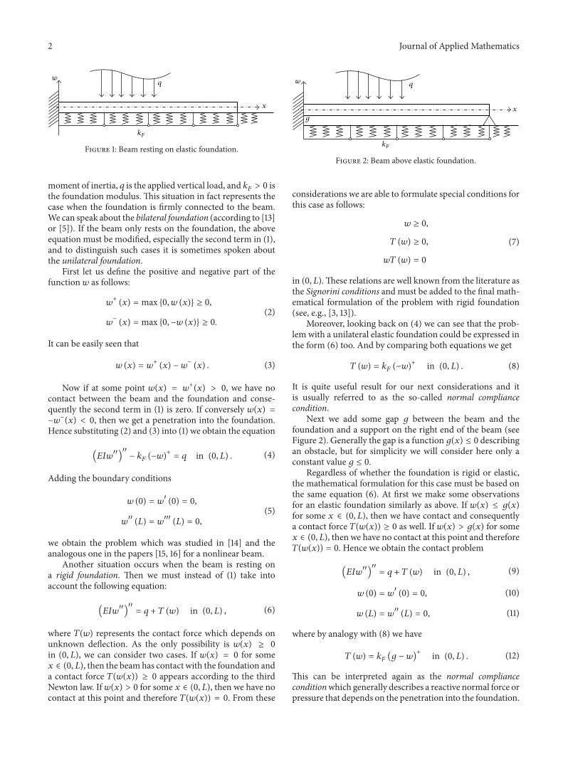
21 Classical Formulations Our considerations will start byrecalling the problem with a beam resting on an elastic foun-dation (see Figure 1) For convenience we will deal initiallywith the Euler-Bernoulli model on Winkler foundation Theequation reads as follows
(11986411986811990810158401015840)10158401015840
+ 119896119865119908 = 119902 in (0 119871) (1)
where 119908 is the deflection of the beam 119871 is the length of thebeam 119864 gt 0 is Youngrsquos elastic modulus 119868 gt 0 is the area
Hindawi Publishing CorporationJournal of Applied MathematicsVolume 2015 Article ID 420649 12 pageshttpdxdoiorg1011552015420649
2 Journal of Applied Mathematics
kF
w
x
q
Figure 1 Beam resting on elastic foundation
moment of inertia 119902 is the applied vertical load and 119896119865gt 0 is
the foundation modulus This situation in fact represents thecase when the foundation is firmly connected to the beamWe can speak about the bilateral foundation (according to [13]or [5]) If the beam only rests on the foundation the aboveequation must be modified especially the second term in (1)and to distinguish such cases it is sometimes spoken aboutthe unilateral foundation
First let us define the positive and negative part of thefunction 119908 as follows
119908+ (119909) = max 0 119908 (119909) ge 0
119908minus (119909) = max 0 minus119908 (119909) ge 0(2)
It can be easily seen that
119908 (119909) = 119908+ (119909) minus 119908minus (119909) (3)
Now if at some point 119908(119909) = 119908+(119909) gt 0 we have nocontact between the beam and the foundation and conse-quently the second term in (1) is zero If conversely 119908(119909) =minus119908minus(119909) lt 0 then we get a penetration into the foundationHence substituting (2) and (3) into (1) we obtain the equation
(11986411986811990810158401015840)10158401015840
minus 119896119865(minus119908)+ = 119902 in (0 119871) (4)
Adding the boundary conditions
119908 (0) = 1199081015840 (0) = 0
11990810158401015840 (119871) = 119908101584010158401015840 (119871) = 0(5)
we obtain the problem which was studied in [14] and theanalogous one in the papers [15 16] for a nonlinear beam
Another situation occurs when the beam is resting ona rigid foundation Then we must instead of (1) take intoaccount the following equation
(11986411986811990810158401015840)10158401015840
= 119902 + 119879 (119908) in (0 119871) (6)
where 119879(119908) represents the contact force which depends onunknown deflection As the only possibility is 119908(119909) ge 0in (0 119871) we can consider two cases If 119908(119909) = 0 for some119909 isin (0 119871) then the beam has contact with the foundation anda contact force 119879(119908(119909)) ge 0 appears according to the thirdNewton law If 119908(119909) gt 0 for some 119909 isin (0 119871) then we have nocontact at this point and therefore 119879(119908(119909)) = 0 From these
g
w
x
q
kF
Figure 2 Beam above elastic foundation
considerations we are able to formulate special conditions forthis case as follows
119908 ge 0
119879 (119908) ge 0
119908119879 (119908) = 0
(7)
in (0 119871)These relations are well known from the literature asthe Signorini conditions and must be added to the final math-ematical formulation of the problem with rigid foundation(see eg [3 13])
Moreover looking back on (4) we can see that the prob-lem with a unilateral elastic foundation could be expressed inthe form (6) too And by comparing both equations we get
119879 (119908) = 119896119865(minus119908)+ in (0 119871) (8)
It is quite useful result for our next considerations and itis usually referred to as the so-called normal compliancecondition
Next we add some gap 119892 between the beam and thefoundation and a support on the right end of the beam (seeFigure 2) Generally the gap is a function 119892(119909) le 0 describingan obstacle but for simplicity we will consider here only aconstant value 119892 le 0
Regardless of whether the foundation is rigid or elasticthe mathematical formulation for this case must be based onthe same equation (6) At first we make some observationsfor an elastic foundation similarly as above If 119908(119909) le 119892(119909)for some 119909 isin (0 119871) then we have contact and consequentlya contact force 119879(119908(119909)) ge 0 as well If 119908(119909) gt 119892(119909) for some119909 isin (0 119871) then we have no contact at this point and therefore119879(119908(119909)) = 0 Hence we obtain the contact problem
(11986411986811990810158401015840)10158401015840
= 119902 + 119879 (119908) in (0 119871) (9)
119908 (0) = 1199081015840 (0) = 0 (10)
119908 (119871) = 11990810158401015840 (119871) = 0 (11)
where by analogy with (8) we have
119879 (119908) = 119896119865(119892 minus 119908)+ in (0 119871) (12)
This can be interpreted again as the normal complianceconditionwhich generally describes a reactive normal force orpressure that depends on the penetration into the foundation
Journal of Applied Mathematics 3
For the case of rigid foundation we must add to (9)ndash(11)the slightly modified Signorini conditions (7)
119908 ge 119892
119879 (119908) ge 0
(119908 minus 119892) 119879 (119908) = 0
(13)
in (0 119871)We can observe that both problems are quite similar and
letting the gap equal zero in the second problem (9)ndash(11) weobtain the mathematical formulation for the first one
Finally adding the support to the right end of the beamwe limit our considerations without loss of generality to thecase when the resultant of acting loads at 119909 = 119871 is negativethat is it is headed downward because for such cases we canobtain a contact between the beam and the support
22 Weak and Variational Formulations After the classicalformulation we now proceed to the variational one which ismore suitable for a numerical solution First we must define asuitable space for test functions According to the boundaryconditions it will be
119881 = V isin 1198672 ((0 119871)) V (0) = V1015840 (0) = 0 = V (119871) (14)
where1198672((0 119871)) is the Sobolev space (see eg [2 3]) Next letus introduce for any 119906 V isin 119881 the notations
119886 (119906 V) = int119871
0
11986411986811990610158401015840V10158401015840d119909
120581 (119906 V) = int119871
0
119896119865119906+V d119909
(119902 V) = int119871
0
119902V d119909
(15)
Evidently 119886(sdot sdot) represents a bilinear form on 119881 times 119881 and (sdot sdot)the inner product in the Lebesgue space 1198712((0 119871))
Thewell-known fact consists in the fact that contact prob-lems can be expressed by means of variational inequalities(see eg [3 13]) For the case with a rigid foundation weintroduce the set of admissible deflections (or test functions)as
119870 = V isin 119881 V ge 119892 in (0 119871) (16)
Using scalar multiplication with functions V minus 119908 we obtainfrom (6)
119886 (119908 V minus 119908) = (119902 V minus 119908) + (119879 (119908) V minus 119908) forallV isin 119870 (17)
From (13) and (16) it follows that
119879 (119908) (V minus 119908) = 119879 (119908) (V minus 119892) + 119879 (119908) (119892 minus 119908)
= 119879 (119908) (V minus 119892) ge 0 forallV isin 119870(18)
and hence the contact problem (9)ndash(11) together with theSignorini conditions (13) can be now formulated as thefollowing variational inequality
Find a function 119908 isin 119870 such that
119886 (119908 V minus 119908) ge (119902 V minus 119908) forallV isin 119870 (19)
For the problem with an elastic deformable foundationthe formulation is obtained by taking the 1198712-inner product of(9) with test functions V isin 119881 After that we obtain
119886 (119908 V) + (minus119879 (119908) V) = (119902 V) forallV isin 119881 (20)
It is quite interesting that for the elastic foundation wereceived the variational equality instead of an inequality asit is usual in contact problems formulations Equation (20)may be rearranged using the relation (12) for contact forcesApplying the notation (15) we get the weak formulation of ourproblem
Find a function 119908 isin 119881 such that
119886 (119908 V) minus 120581 (119892 minus 119908 V) = (119902 V) forallV isin 119881 (21)
This is of course nonlinear problem as it shows the secondterm in (21)
Next let us associate the energy functional
Π119861(V) = 1
2int119871
0
119864119868 (V10158401015840)2
d119909 minus int119871
0
119902V d119909
= 12119886 (V V) minus (119902 V)
(22)
with the Euler-Bernoulli beamThen the problem (19) can beequivalently expressed using minimization problem
Find 119908 isin 119870 such that
Π119861(119908) = min
Visin119870Π119861(V) (23)
We are able also to construct the functional of totalpotential energy Π for the problem (21) Let us introduce theenergy of foundation reaction forces by
Π119865(V) = 1
2int119871
0
119896119865(V+)2 d119909 (24)
Then we have
Π (V) = Π119861(V) + Π
119865(119892 minus V)
= 12int119871
0
119864119868 (V10158401015840)2
d119909 + 12int119871
0
119896119865((119892 minus V)+)
2
d119909
minus int119871
0
119902V d119909
(25)
and the minimization problem reads as follows
Find 119908 isin 119881 such that
Π (119908) = minVisin119881
Π (V) (26)
This problem is convex and differentiable in the sense ofGateaux This implies the equivalence (26) to the previousformulation (21)
4 Journal of Applied Mathematics
3 Nonlinear Gao Beam
In the previous section we were concerned for simplicitywith the standard Euler-Bernoulli beammodel But ourmaininterest in this paper will be to study contact for the nonlinearbeam model which was proposed by Gao in [1 17] We willmention this model here only briefly and only the mostsimple version (with zero axial force) given by a fourth-ordernonlinear differential equation
1198641198681199081015840101584010158401015840 minus 119864120572 (1199081015840)2
11990810158401015840 = 119891 in (0 119871) (27)
The beam has a constant stiffness given by an elastic modulus119864 and a constant area moment of inertia 119868 Its length is 119871 andthickness is ℎ measured from the 119909-axis and therefore thefull thickness will be 2ℎ The width of the beam is consideredas a unit The transverse load is denoted by 119902(119909) and 119908(119909)describes the deflection of the beam at a position 119909 Equation(27) has the following built-in relationships
119868 = 23ℎ3
120572 = 3ℎ (1 minus ]2)
119891 = (1 minus ]2) 119902
(28)
where ] denotes the Poisson ratio Boundary conditionsremain the same as before that is (10)-(11) For the load 119891we will assume the same as in the previous section for load 119902that is the resultant at 119909 = 119871must be negative
Of course the considerations concerning the contact withfoundation that we have made before remain valid Hencethe classical formulation for the contact problem with a rigidfoundation reads as follows
1198641198681199081015840101584010158401015840 minus 119864120572 (1199081015840)2
11990810158401015840 = 119891 + (1 minus ]2) 119879 (119908)
in (0 119871)
119908 (0) = 1199081015840 (0) = 0
119908 (119871) = 11990810158401015840 (119871) = 0
119908 ge 119892
119879 (119908) ge 0
(119908 minus 119892) 119879 (119908) = 0
(29)
in (0 119871) and for an elastic deformable foundation we have
1198641198681199081015840101584010158401015840 minus 119864120572 (1199081015840)2
11990810158401015840 minus 119888119865(119892 minus 119908)+ = 119891
in (0 119871)
119908 (0) = 1199081015840 (0) = 0
119908 (119871) = 11990810158401015840 (119871) = 0
(30)
with 119888119865= (1 minus ]2)119896
119865
Variational formulation for this problem we can get by asimilar way as above Let us define the functionals of totalpotential energy for our problems by adding the nonlineartermΠ
119873to the functionalΠ
119861orΠ from the previous section
with substituting 119891 for 119902 and 119888119865for 119896119865as
Π1(V) = Π (V) + Π
119873(V) = Π (V) + int
119871
0
11986412057212
(V1015840)4
d119909 (31)
This is a nonlinear convex functional Hence we can againformulate the minimization problem for a deformable foun-dation as follows
Find 119908 isin 119881 such that
Π1(119908) = min
Visin119881Π1(V) (32)
and this problem is due to its convexity equivalent to thefollowing nonlinear variational equation
Find a function 119908 isin 119881 such that
119886 (119908 V) + 120587 (119908 V) minus 120581 (119892 minus 119908 V) = (119891 V) forallV isin 119881 (33)
where we denoted
120587 (119908 V) = Π1015840119873(119908 V) = int
119871
0
1198641205723(1199081015840)3
V1015840d119909 (34)
and Π1015840119873(119908 V) means the Gateaux differential of Π
119873at the
point 119908 in the direction V We of course substituted 119888119865for 119896119865
in 120581(sdot sdot) as wellAnalogously we get for a rigid foundation the next two
problems
Find 119908 isin 119870 such that
Π2(119908) = min
Visin119870Π2(V) (35)
where (again substituting 119891 for 119902)
Π2(V) = Π
119861(V) + Π
119873(V) = Π
119861(V) + int
119871
0
11986412057212
(V1015840)4
d119909 (36)
and (equivalently)
Find a function 119908 isin 119870 such that
119886 (119908 V minus 119908) + 120587 (119908 V minus 119908) ge (119891 V minus 119908) forallV isin 119870 (37)
4 Optimal Control Problem
Our approach will be based on an optimal problem formula-tion and solutionThe idea is due to themethod applied in thepapers [4] [7] or [8] the authors call it the control variationalmethod
First of all let us recall briefly the concept of the optimalcontrol of elliptic equations by the right hand side (see eg[11 12]) Let 119880ad be a subset of a space of controls 119880 and let119861 be a linear continuous operator from 119880 into 1198811015840 where 1198811015840is the dual space to a Hilbert space 119881 For any given 119906 isin 119880adand any 119891 isin 1198811015840 we will define the problem
Journal of Applied Mathematics 5
Find a function 119908 = 119908(119906) such that
(11986411986811990810158401015840)10158401015840
= 119891 + 119861119906 in (0 119871)
119908 (0) = 1199081015840 (0) = 0
119908 (119871) = 11990810158401015840 (119871) = 0
(38)
Subset 119880ad is called the set of admissible controls and (38) isthe classical formulation of the state problem Such type ofproblems belongs to problems with distributed control whichmeans that 119906 isin 119880ad acts in the whole interval (0 119871)
Next we will proceed to the variational formulation forthe state problem which will be in most cases better suitedthan the previous one At the same time we will specify moreprecisely its setting Let 119880ad be a nonempty bounded closedconvex subset of a reflexive Banach space 119880 and let 119861 be alinear continuous mapping from119880 to1198811015840 For any 119906 isin 119880ad wewill want to
Find a function 119908 = 119908(119906) isin 119881 such that
119886 (119908 V) = ⟨119891 + 119861119906 V⟩1198811015840times119881
forallV isin 119881 (39)
where ⟨sdot sdot⟩1198811015840times119881
denotes the duality pairing between 1198811015840 and119881
Let a cost (or criterion) functional 119869 119881times119880 997891rarr R be givenand let it be weakly lower semicontinuous that is
119908119899 119908
119906119899 119906
as 119899 997888rarr +infin
997904rArr lim inf119899rarr+infin
119869 (119908119899 119906119899) ge 119869 (119908 119906)
(40)
Now let us define the resulting optimal control problem
Find a function 119906lowast isin 119880ad such that
119869 (119908 (119906lowast) 119906lowast) = min119906isin119880ad
119869 (119908 (119906) 119906) (41)
where 119908(119906) isin 119881 solves the state problem (39)It is important that we are able to prove the following
proposition (using arguments from [11] or [12])
Theorem 1 The problem (41) has under the abovementionedassumptions at least one solution
Proof Let
119902 = inf119906isin119880ad
119869 (119908 (119906) 119906) = lim119899rarr+infin
119869 (119908 (119906119899) 119906119899) (42)
that is 119906119899 is a minimizing sequence of (41) As 119880ad is
bounded and119880 is reflexive there exists a subsequence 1199061198991015840 sub
119906119899 such that
1199061198991015840 119906lowast isin 119880ad (43)
At the same time 1199081198991015840 = 119908(119906
1198991015840) isin 119881 which are the solution of
119886 (1199081198991015840 V) = ⟨119891 + 119861119906
1198991015840 V⟩1198811015840times119881
forallV isin 119881 (44)
are bounded as well and we may assume that
1199081198991015840 119908lowast isin 119881 (45)
Passing to the limit with 1198991015840 rarr +infin in (44) we see that
119886 (119908lowast V) = ⟨119891 + 119861119906lowast V⟩1198811015840times119881
forallV isin 119881 (46)
that is 119908lowast = 119908(119906lowast) On the other hand from (40)119902 = lim1198991015840rarr+infin
119869 (119908 (1199061198991015840) 1199061198991015840) = lim inf1198991015840rarr+infin
119869 (119908 (1199061198991015840) 1199061198991015840)
ge 119869 (119908 (119906lowast) 119906lowast) ge 119902(47)
that is 119906lowast is a solution of (41)
Finally we will deal with optimality conditions for ouroptimal control problem In the text below we will use forsimplicity the abbreviation
119860119908 = (11986411986811990810158401015840)10158401015840 (48)
with the linear continuous operator 119860 from 119881 to 1198811015840 The keyidea lies in the fact that the problem (41) can be considered asa constrained minimization problem For this purpose let usdefine the set
119882 = (119908 119906) isin 119881 times 119880ad 119860119908 = 119891 + 119861119906 (49)
It is evident thatmin119906isin119880ad
119869 (119908 (119906) 119906) = min(119908119906)isin119882
119869 (119908 119906) (50)
At the same time we can see that(119908 119906) isin 119882 lArrrArr ⟨119891 + 119861119906 minus 119860119908 119901⟩
1198811015840times119881
= 0
forall119901 isin 119881(51)
Let us denoteΦ(119908 119906 119901) = ⟨119891 + 119861119906 minus 119860119908 119901⟩
1198811015840times119881
forall119908 isin 119881 119906 isin 119880ad 119901 isin 119881(52)
Then it is easy to see that
(119908 119906) 997891997888rarr sup119901isin119881
Φ(119908 119906 119901) (53)
is the indicator function of the set119882 This implies
min(119908119906)isin119882
119869 (119908 119906)
= min(119908119906)isin119881times119880ad
sup119901isin119881
119869 (119908 119906) + Φ (119908 119906 119901)(54)
and consequently we can define the Lagrangian L with aLagrange multiplier 119901
L (119908 119906 119901) = 119869 (119908 119906) + Φ (119908 119906 119901)
forall119908 isin 119881 119906 isin 119880ad 119901 isin 119881(55)
Let us consider a saddle point (119908 119906 119901) isin 119881 times 119880ad times 119881 ofL The following proposition is a known characterization ofsaddle points
6 Journal of Applied Mathematics
Lemma 2 (see eg [18 Chapter VI Proposition 12]) Anelement (119911 120582) isin 119885 times Λ is a saddle point of a Lagrangian Lif and only if
min119911isin119885
sup120582isinΛ
L (119911 120582) = L (119911 120582) = max120582isinΛ
inf119911isin119885
L (119911 120582) (56)
Taking into account the definition (55) and Lemma 2 itcan be seen that
L (119908 119906 119901) = min(119908119906)isin119881times119880ad
sup119901isin119881
L (119908 119906 119901)
= min(119908119906)isin119882
119869 (119908 119906) = 119869 (119908 119906) (57)
From here it is evident that (119908 119906) is a solution of (41)Next let us suppose that 119869 is differentiable Then from the
saddle point definition it follows that
⟨nabla119908L (119908 119906 119901) 119908⟩
1198811015840times119881
= 0 forall119908 isin 119881 (58)
⟨nabla119906L (119908 119906 119901) 119906 minus 119906⟩
1198801015840times119880
ge 0 forall119906 isin 119880ad (59)
⟨nabla119901L (119908 119906 119901) 119901⟩
1198811015840times119881
= 0 forall119901 isin 119881 (60)
From the first condition (58) we get
⟨nabla119908119869 (119908 119906) 119908⟩
1198811015840times119881
minus ⟨119860119908 119901⟩1198811015840times119881
= 0 forall119908 isin 119881 (61)
whereas the last condition (60) gives
119860119908 = 119891 + 119861119906 (62)
which means that (119908 119906) isin 119882 From (61) using definition ofthe adjoint operator 119860lowast to the operator 119860 we have
119860lowast119901 = nabla119908119869 (119908 119906) (63)
which is the so-called adjoint equation We can see that itssolution 119901 called the adjoint state is nothing else but theoptimal value of the Lagrange multiplier associated with theconstraint given by the set 119882 Finally the second condition(59) can be according to (52) written as
⟨nabla119906119869 (119908 119906) 119906 minus 119906⟩
1198801015840times119880
+ ⟨119861lowast119901 119906 minus 119906⟩1198801015840times119880
ge 0
forall119906 isin 119880ad(64)
where119861lowast is the adjoint operator to119861The three relations (62)ndash(64) form the requested optimality conditions
Later it will be important to know the gradient of the costfunctional 119869 To this purpose let us denote
119868 (119906) = 119869 (119908 (119906) 119906) forall119906 isin 119880ad (65)
and analyze properties of the mapping 119906 997891rarr 119868(119906) It is known(eg from the monographs [11 12]) that
⟨nabla119906119868 (119906) 119911⟩
1198801015840times119880
= ⟨119861lowast119901 119911⟩1198801015840times119880
+ ⟨nabla119906119869 (119908 119906) 119911⟩
1198801015840times119880
forall119911 isin 119880(66)
where 119901 is a solution to the adjoint equation and it implies
nabla119906119868 (119906) = 119861lowast119901 + nabla
119906119869 (119908 119906) 119906 isin 119880ad (67)
5 Transformation to OptimalControl Problems
51 Problem with a Deformable Foundation Now let usreturn to our contact problems (32) and (35) Our next stepswill be transformations of the energy functionalsΠ
1and Π
2
Main attention will be focused on the first case as the secondone with a rigid foundation is for many years well known inthe literature (eg [2 13])
First let us perform some rearrangement of its part Π119861
given by (22) For this purpose let the state problem be (39)with operator 119861 as identity that is
Find 119908 = 119908(119906) isin 119881 such that
119886 (119908 V) = (119891 + 119906 V) forallV isin 119881 (68)
Let 119908 isin 119881 be the (unique) solution of the state problem forthe control variable 119906 = 0 that is 119908 fulfills
119886 (119908 V) = (119891 V) forallV isin 119881 (69)
Then substituting119891 for 119902 and using (68) and (69) we find that
Π119861(119908) = 1
2119886 (119908 119908) minus (119891 119908) = 1
2(119906 119908) minus 1
2(119891 119908)
= 12(119906 119908) minus 1
2119886 (119908 119908)
= 12(119906 119908) minus 1
2(119891 + 119906 119908)
= 12(119906 119908 minus 119908) minus 1
2(119891 119908)
(70)
As the last term in (70) is in fact a constant we can omitit from the viewpoint of minimization and define the newfunctional as
119869 (119908 119906) = 12(119906 119908 minus 119908) = 1
2int119871
0
119906 (119908 minus 119908) d119909 (71)
We still have not defined the set119880ad Fromaphysical pointof view it seems to be a good choice 119880 = 1198712((0 119871)) followedby
119880ad = 119906 isin 1198712 ((0 119871)) |119906 (119909)| le 119862 ae in (0 119871) (72)
for some positive constant 119862 (depending on the beamcompliance) as we do not want to break the beam
Thus the cost functional 1198691will be therefore the following
conversion of Π1
1198691(119908 119906) = 119869 (119908 119906) + Π
119873(119908) + Π
119865(119892 minus 119908)
= 12int119871
0
119906 (119908 minus 119908) d119909 + 121198641205726int119871
0
(1199081015840)4
d119909
+ 12119888119865int119871
0
((119892 minus 119908)+)2
d119909
(73)
Finally we get the first optimal control problem
Journal of Applied Mathematics 7
Find 119906lowast isin 119880ad such that
1198691(119908 (119906lowast) 119906lowast) = min
119906isin119880ad1198691(119908 (119906) 119906) (74)
where 119908(119906) isin 119881 solves the state problem (68)We can state the following proposition about a relation
between the problems (74) and (32)
Theorem 3 Let 119906lowast solve the optimal control problem (74)Then119908lowast = 119908(119906lowast) is a solution of the corresponding variationalproblem (32) providing that the constant 119862 in (72) is bigenough
Proof Let (119908lowast 119906lowast) isin 119881 times 119880ad be an optimal pair of theproblem (74) Let us consider admissible pairs of the form(119908lowast + 119905(119910 minus 119908lowast) 119906lowast + 119905(119911 minus 119906lowast)) for any 119905 isin [minus1 1] 119911 isin 119880adand any 119910 isin 119881 satisfying the state equation (68)
119886 (119908lowast + 119905 (119910 minus 119908lowast) V) = (119891 + 119906lowast + 119905 (119911 minus 119906lowast) V)
forallV isin 119881(75)
As
119886 (119908lowast V) = (119891 + 119906lowast V) forallV isin 119881 (76)
we get after substitution that (119910 119911)must fulfill
119886 (119910 minus 119908lowast V) = (119911 minus 119906lowast V) forallV isin 119881 (77)
or
119886 (119910 V) = (119891 + 119911 V) forallV isin 119881 (78)
From the optimality of (119908lowast 119906lowast) we have
1198691(119908lowast 119906lowast) le 119869
1(119908 119906) forall (119908 119906) isin 119881 times 119880ad (79)
Substituting the above mentioned expressions for119908 and 119906weget after some manipulations
Π119873(119908lowast) + Π
119865(119892 minus 119908lowast)
le 1199052(119911 minus 119906lowast 119908lowast) + 119905
2(119906lowast 119910 minus 119908lowast)
minus 1199052(119911 minus 119906lowast 119908) + 1199052
2(119911 minus 119906lowast 119910 minus 119908lowast)
+ Π119873(119908lowast + 119905 (119910 minus 119908lowast))
+ Π119865(119892 minus 119908lowast minus 119905 (119910 minus 119908lowast))
(80)
Dividing this inequality by 119905 gt 0 and letting 119905 rarr 0+ weobtain (using (76) (77) and (34)) that
0 le 12(119911 minus 119906lowast 119908lowast) + 1
2(119906lowast 119910 minus 119908lowast) minus 1
2(119911 minus 119906lowast 119908)
+ Π1015840119873(119908lowast 119910 minus 119908lowast) + Π1015840
119865(119892 minus 119908lowast 119910 minus 119908lowast)
= 119886 (119908lowast 119910 minus 119908lowast) minus (119891 119910 minus 119908lowast) + 120587 (119908lowast 119910 minus 119908lowast)
minus 120581 (119892 minus 119908lowast 119910 minus 119908lowast)
(81)
for any (119910 119911) isin 119881 times 119880ad satisfying (78) As we can take 119905 isin R
positive as well as negative this relation gives us the desiredequality (33)which is equivalent to theminimization problem(32)
Finally let us notice that the assumption regarding theconstant 119862 from the definition of 119880ad means that 119906lowast and 119911were inner points of the set 119880ad
Theorem 4 The variational problem (32) has exactly onesolution
Proof The proof follows immediately from the fact that thefunctional Π
1is strictly convex on 119881 This property can be
easily deduced from the inequality
exist119888 gt 0 V le 119888 10038171003817100381710038171003817V101584010038171003817100381710038171003817 forallV isin 119881 (82)
where sdot denotes the 1198712((0 119871))-norm that is V = radic(V V)
As a consequence ofTheorems 1 3 and 4 we obtained thefollowing proposition
Corollary 5 The optimal control problem (74) has exactly onesolution under the assumption that the constant119862 in (72) is bigenough
Proof As the functional 1198691(119908 119906) is weakly lower semicon-
tinuous and the set 119880ad in (74) is a bounded subset of119880 = 1198712((0 119871)) we get from Theorem 1 that (74) has at leastone solution For every such solution (119908(119906lowast) 119906lowast) its firstcomponent 119908(119906lowast) = 119908lowast solves the associated variationalproblem (32) byTheorem 3 But (32) has exactly one solutionby Theorem 4 whereas the mapping 119906 997891rarr 119908(119906) is linearaccording to the state equation (68) This completes theproof
52 Problem with a Rigid Foundation The state problemremains formally the same as before that is (68) But now wemust respect the contact conditions (13) especially 119908 ge 119892Of course a solution 119908(119906) to the state equation generallydoes not satisfy such a condition for arbitrary 119906 In order toguarantee it the set 119880ad has to be properly redefined
Using notation (48) we have from (38)
119860119908 = 119891 + 119906 (83)
and it follows that
119908 = 119860minus1119891 + 119860minus1119906 = 119908 + 119860minus1119906 ge 119892 (84)
Hence let us define
119880ad = 119906 isin 1198712 ((0 119871)) 119860minus1119906 ge 119892 minus 119908 |119906|
le 119862 ae in (0 119871) (85)
Obviously for any 119906 isin 119880ad we have a unique solution 119908 =119908(119906) of the problem (68) and it fulfills119908 ge 119892 that is it lies in119870
8 Journal of Applied Mathematics
The cost functional 1198692will be the following conversion of
Π2
1198692(119908 119906) = 119869 (119908 119906) + Π
119873(119908)
= 12int119871
0
119906 (119908 minus 119908) d119909 + 121198641205726int119871
0
(1199081015840)4
d119909(86)
Finally we get the second optimal control problem
Find 119906lowast isin 119880ad such that
1198692(119908 (119906lowast) 119906lowast) = min
119906isin119880ad1198692(119908 (119906) 119906) (87)
where 119908(119906) isin 119870 solves the state equation (68)Now it is important to establish a proposition about the
equivalence of the problems (87) and (35)
Theorem 6 Let 119906lowast solve the optimal control problem (87)Then119908lowast = 119908(119906lowast) is a solution of the corresponding variationalproblem (35) providing that the constant 119862 in (85) is bigenough
Proof Let (119908lowast 119906lowast) isin 119881 times 119880ad be an optimal pair of theproblem (87) Let us consider admissible pairs of the form(119908lowast + 119905(119910minus119908lowast) 119906lowast + 119905(119911minus119906lowast)) for any 119905 isin [0 1] 119911 isin 119880ad andany 119910 isin 119870 satisfying the state equation (68)
Using similar arguments as in the previous proof ofTheorem 3 we come to the following inequality
0 le 12(119911 minus 119906lowast 119908lowast) + 1
2(119906lowast 119910 minus 119908lowast) minus 1
2(119911 minus 119906lowast 119908)
+ Π1015840119873(119908lowast 119910 minus 119908lowast)
= 119886 (119908lowast 119910 minus 119908lowast) minus (119891 119910 minus 119908lowast) + 120587 (119908lowast 119910 minus 119908lowast)
forall (119910 119911) isin 119870 times 119880ad
(88)
As 119905 isin [0 1] we obtain the final result in the form
119886 (119908lowast 119910 minus 119908lowast) + 120587 (119908lowast 119910 minus 119908lowast) ge (119891 119910 minus 119908lowast)
forall119910 isin 119870(89)
which is the requested problem (37)
Finally we may use almost the same arguments as in theprevious paragraph to obtain the following proposition
Corollary 7 The optimal control problem (87) has exactly onesolution
Remark 8 (construction of the set 119880119886119889) Determination of
the set (72) does not make any trouble unlike the case withsomewhat abstract definition (85) But these difficulties canbe solved by using a penalization especially by means ofbarrier function method Hence we add to the functional1198692(119908 119906) the expression
119861120576(119908) = 120576 1
119908 minus 119892 120576 gt 0 119908 isin 119870 (90)
and take the limit for 120576 0 (see eg [2 Chapter 2])
6 Numerical Realization and Algorithms
Next some approximations of our problems are needed sinceexact solutions are not available We start with the generalproblem (41) Instead of the state problem (39) its full finiteelement discretization must be taken into account that isnot only discretization of function spaces but also approxima-tions of the linear form and themapping 119861 denoted by119891
ℎ 119861ℎ
respectively Here ℎ denotes the discretization parameterwhich in the finite element interpretation is given as themaximal diameter over all elements from the current finiteelement mesh For our purposes we do not need numericalcomputations of the bilinear form 119886(sdot sdot) (we will discuss it abit later)
Let 119881ℎsub 119881 and 119880
ℎsub 119880 be finite-dimensional subspaces
of 119881 and 119880 respectively and let 119880ℎad sub 119880ℎ be a nonemptyclosed convex and bounded subset of 119880 that is we do notassume that necessarily 119880ℎad sub 119880ad
The state problem (39) is now replaced by its finiteelement approximation
Find 119908ℎ= 119908ℎ(119906ℎ) isin 119881ℎsuch that
119886 (119908ℎ(119906ℎ) Vℎ) = ⟨119891
ℎ+ 119861ℎ119906ℎ Vℎ⟩ℎ
forallVℎisin 119881ℎ (91)
where ⟨sdot sdot⟩ℎis the duality pairing between 1198811015840
ℎand 119881
ℎ
Let 119869ℎ 119881ℎtimes 119880ℎ997891rarr R be a cost functional which is lower
semicontinuous on 119881ℎtimes 119880ℎ that is
119908119896ℎ997888rarr 119908
ℎ
119906119896ℎ997888rarr 119906ℎ
as 119896 997888rarr +infin
997904rArr lim inf119896rarr+infin
119869ℎ(119908119896ℎ 119906119896ℎ) ge 119869ℎ(119908ℎ 119906ℎ)
(92)
By the approximation of the problem (41) we will understandthe problem
Find a function 119906lowastℎisin 119880ℎad such that
119869ℎ(119908ℎ(119906lowastℎ) 119906lowastℎ) = min119906ℎisin119880ℎ
ad
119869ℎ(119908ℎ(119906ℎ) 119906ℎ) (93)
where 119908ℎ(119906ℎ) isin 119881ℎsolves the discretized state problem (91)
The bilinear form 119886 is continuous and 119881-elliptic If we areallowed to assume 119891
ℎisin 1198811015840ℎand 119861
ℎisin L(119880
ℎ 1198811015840ℎ) then the
discretized state problem (91) has exactly one solution for any119906ℎisin 119880ℎ Let moreover (92) hold and then it is easy to prove
that the optimization problem (93) has at least one solution119906lowastℎNow we want to establish a relation between the contin-
uous problem (41) and the discrete problem (93) as ℎ rarr0+ This analysis is important for computations but we donot intend to go into details here since they are somewhatcomprehensive
In this sectionwe establishmatrix formulation of the opti-mal control problem (74) To this purpose let discretization
Journal of Applied Mathematics 9
parameter ℎ be fixed let two divisions of [0 119871] into119873(ℎ) and119872(ℎ) subintervals be done and let
dim119881ℎ= 119873 (ℎ) = 119873
dim119880ℎ= 119872(ℎ) = 119872
(94)
Furthermore let
119881ℎ= span 120593
1 1205932 120593
119873
119880ℎ= span 120595
1 1205952 120595
119872
(95)
that is 120593119894119873119894=1
120595119895119872119895=1
are basis functions of 119881ℎ 119880ℎ respec-
tively Then any function 119908ℎisin 119881ℎcan be expressed as
119908ℎ(119909) =
119873
sum119894=1
120572119894120593119894(119909) 120572
119894isin R 119894 = 1 119873 (96)
Analogously we have
119906ℎ(119909) =
119872
sum119895=1
120573119895120595119895(119909) 120573
119895isin R 119895 = 1 119872 (97)
The Galerkin method is based on the following idea wesubstitute expression (96) and (97) into (68) and then as testfunctions V
ℎsuccessively choose basis functions 120593
1 120593
119873
This way we obtain for the given vector 120573 = (120573119895)119872119895=1
isin R119872
(representing a given control parameter value) the system oflinear algebraic equations with the unknown 120572 = (120572
119894)119873119894=1
isinR119873
K120572 = f + B120573 (98)
where we denoted
K = (119896119894119895)119873
119894119895=1isin R119873times119873 119896
119894119895= 119886 (120593
119895 120593119894)
B = (119887119894119895)119895=1119872
119894=1119873isin R119873times119872 119887
119894119895= ⟨119861ℎ120595119895 120593119894⟩ℎ
f = (119891119894)119873119894=1
isin R119873 119891
119894= ⟨119891ℎ 120593119894⟩ℎ
(99)
The matrix K is the well-known stiffness matrix and f is theload vector
The finite element method usually works with the so-called Courant basis functions which are characterized by thefollowing ldquo120575
119894119895-propertyrdquo
120594119894(119909119895) =
1 if 119894 = 119895
0 if 119894 = 119895(100)
Applying this to the functions from 120593119894119873119894=1
120595119895119872119895=1
we can seeaccording to (96) and (97)
120572119894= 119908ℎ(119909119894) equiv 119908119894
120573119895= 119906ℎ(119909119895) equiv 119906119895
(101)
Next defining
w = (119908119894)119873119894=1
isin R119873
u = (119906119894)119872119894=1
isin R119872
(102)
it is possible to rewrite the system (98) in the new and moreusual form
Kw = f + Bu (103)
The previous procedure is quite general hence for nextcalculations we should specify the finite element basis moreprecisely The standard beam elements are chosen for thebeam and it is well known that they are working withHermitian shape functions The system 120593
119894119873119894=1
is createdby linking of appropriate shape functions from adjacentsubintervals This leads to the following description of thefinite element space
119881ℎ= 119908ℎisin 1198621 ((0 119871)) V
ℎ
1003816100381610038161003816119870119894
isin 1198753(119870119894) forall119870119894 119908ℎ(0)
= 1199081015840ℎ(0) = 0 = 119908
ℎ(119871)
(104)
where 119870119894denotes 119894th subinterval of (0 119871) and 119875
3(119870119894) means
the space of cubic polynomials defined on 119870119894 Values of the
bilinear form 119886(sdot sdot) for constant values 119864 and 119868 are then doneexactly that is no numerical integration is needed For moredetails see for example [19 Chapter 5]
Construction of the set 119880ℎuses here the same system of
subintervals as119881ℎ that is value119872 = 119873 andworkswith linear
shape functions defined on them Therefore we have
119880ℎ= 119906ℎisin 1198620 ((0 119871)) 119906
ℎ
1003816100381610038161003816119870119894
isin 1198751(119870119894) forall119870119894 (105)
Next let us formally define two isomorphisms
I1 119881ℎ997888rarr R
119873 I1119908ℎ= w
I2 119880ℎ997888rarr R
119872 I2119906ℎ= u
(106)
Then the discrete control variable u belongs to the set
Uad = u isinR119872 Iminus12u isin 119880ℎad (107)
Similarly we are able to construct the algebraic representationof 119869ℎas follows
119865 (w u) = 119869ℎ(Iminus11wIminus12u) (108)
where 119865 is a multivariable function Then the optimizationproblem (93) for a fixed parameter ℎ can be equivalentlyexpressed as follows
Find a vector ulowast isin Uad such that
119865 (w (ulowast) ulowast) = minuisinUad
119865 (w (u) u) (109)
where w(u) isin R119873 solves the linear system (103) This formu-lation represents a nonlinear programming problem
10 Journal of Applied Mathematics
0 01 02 03 04 05 06 07 08 09 1 0 01 02 03 04 05 06 07 08 09 1
minus16
minus14
minus12
minus10
minus8
minus6
minus4
minus2
0
minus16
minus14
minus12
minus10
minus8
minus6
minus4
minus2
0
times10minus3 times10minus3
Figure 3 Results of Examples 1 and 2
Remark 9 (construction of the set U119886119889) As the definition
(107) is rather formal some comment is needed especiallyfor the case with rigid foundation Most algorithms can keepthe constraints like V ge 119892 providing that an initial guesssatisfies this condition Such starting guess can be constructedin our problems rather easily For instance let the load 119891 benonpositive functionThen we get119908 le 0 as well and there aretwo possible cases In the first one we have119908 ge 119892 and then wecan put 119906init = 0 In the second case we have in some points119908 lt 119892 Then we can try 119906init = minus120574119891 for some value 120574 gt 0 suchthat the total load 119891 + 119906 causes the deflection 119908 ge 119892 Usuallyjust a few attempts are enough
Remark 10 (solving the nonlinear programming problem(109)) There are two good ways of how to solve the problem(109) The first one consists in using some gradient methodFor this purpose of course we need to compute gradient ofthe cost functional 119869
1or 1198692at any point It can be done by
means of adjoint state as it was established in (66) and (67)Returning to the optimality condition (63) we can write theadjoint equation for 119869
1in the weak form as follows
119886 (119901 V) = 12(119906 V) + 120587 (119908 V) minus 120581 (119892 minus 119908 V) forallV isin 119881 (110)
while in the case of 1198692the equation remains almost the same
only the last term on the right hand side vanishes Solvingthis equation we get the adjoint state 119901 and then the requiredgradient by (67)
nabla119868 (119906) = 119901 (119906) + 12(119908 (119906) minus 119908) 119906 isin 119880ad (111)
Let us notice that instead of using penalization techniquesas it was mentioned in Remark 8 we can more preferablyuse interior-pointmethods (see eg [20]) particularly for thecontact with Signorini conditions
7 Examples
This section presents four examples which are intended todemonstrate the above explained theory and methods Inaddition to the Gao beam model we will present also resultsfor the classical Euler-Bernoulli beammodel for comparisonAs the nonlinear beam model is tougher than the classicalone the upper point curves show the results for theGao beamand lower point curves are the results for the Euler-Bernoullibeam Beams have always the left end fixed and the right endsimply supported as it was considered before (see Figure 2)
The common data are as follows119871 = 1m ℎ = 01m 119868 = 0666667 times 10minus3m4 ] = 03and 119892 = 001mNumber of finite elements = 40
Example 1 (contact with normal compliance condition)Consider the following
Input data 119902 = 5 times 107N 119864 = 3 times 1010 Pa 119864119868 =2 times 107Nm2 and 119896
119865= 2 times 107Nmminus3
Significant results see the left half of Figure 3E-B beam maximal deflection minus00135m contactzone [0375 0775]Gao beam maximal deflection minus00123m contactzone [0425 0725]
Example 2 (contact with normal compliance condition)Consider the following
Smaller load than in Example 1Input data 119902 = 38 times 107N 119864 = 3 times 1010 Pa 119864119868 =2 times 107Nm2 and 119896
119865= 2 times 107Nmminus3
Significant results see the right half of Figure 3E-B beam maximal deflection minus00103m contactzone [0525 0625]
Journal of Applied Mathematics 11
0 01 02 03 04 05 06 07 08 09 1 0 01 02 03 04 05 06 07 08 09 1
minus16
minus14
minus12
minus10
minus8
minus6
minus4
minus2
0
minus16
minus14
minus12
minus10
minus8
minus6
minus4
minus2
0times10minus3 times10minus3
Figure 4 Results of Examples 3 and 4
Gao beam maximal deflection minus00094m contactzone 0
Example 3 (contact with normal compliance condition)Consider the following
Larger foundation stiffness than in Example 1Input data 119902 = 5 times 107N 119864 = 3 times 1010 Pa 119864119868 =2 times 107Nm2 and 119896
119865= 2 times 1011Nmminus3
Significant results see the left half of Figure 4E-B beam maximal deflection minus00104m contactzone [0500 0650]Gao beam maximal deflection minus00103m contactzone [0525 0625]
Example 4 (contact with Signorini conditions) Consider thefollowing
Input data 119902 = 5 times 107N 119864 = 3 times 1010 Pa and 119864119868 =2 times 107Nm2Significant results see the right half of Figure 4E-B beam maximal deflection minus00100m contactzone [0565 0585]Gao beam maximal deflection minus00100m contactzone [0565 0585]
Numerical computations were realized using MATLAB
8 Conclusions
We presented here quite promising methods to solve contactproblem for the Gao beam and an obstacle especially adeformable or a rigid foundation As a result we received anoptimal control problem with following properties
(i) State problem is always linear nonlinearities areldquohiddenrdquo in control variable 119906
(ii) Objective functional has a ldquohandyrdquo form since thetotal potential energy of the system is convex
Hence both optimal control problems are very suitable froma computational point of view
Numerical experiments show us that the Gao beam istougher than the classical beam Computations were ofcourse somewhat longer for the nonlinear beam Anotherobservation is in a good agreement with theoretical results(see [5 6]) for increasing obstacle toughness 119896
119865we can
observe a numerical convergence of results for normal com-pliance contact problems to results for the correspondingSignorini contact problem
Conflict of Interests
The authors declare that there is no conflict of interestsregarding the publication of this paper
References
[1] D Y Gao ldquoNonlinear elastic beam theory with applicationin contact problems and variational approachesrdquo MechanicsResearch Communications vol 23 no 1 pp 11ndash17 1996
[2] R Glowinski J-L Lions and R TremolieresNumerical Analy-sis of Variational Inequalities North-Holland Amsterdam TheNetherlands 1981
[3] N Kikuchi and J T Oden Contact Problems in Elasticity AStudy of Variational Inequalities and Finite Element MethodsSIAM Philadelphia Pa USA 1988
[4] M Sofonea and D Tiba ldquoThe control variational method forcontact of Euler-Bernoulli beamsrdquo Bulletin of the Transilva-nia University of Brasov Series III Mathematics InformaticsPhysics vol 2 pp 127ndash136 2009
[5] M Shillor M Sofonea and J J Telega Models and Analysis ofQuasistatic Contact Variational Methods Springer 2004
[6] M Sofonea and A Matei Mathematical Models in ContactMechanics Lecture Note Series 398 London MathematicalSociety Cambridge University Press 2012
12 Journal of Applied Mathematics
[7] M Sofonea and D Tiba ldquoThe control variational method forelastic contact problemsrdquo Annals of the Academy of RomanianScientists Series on Mathematics and its Applications vol 2 no1 pp 99ndash122 2010
[8] M Barboteu M Sofonea and D Tiba ldquoThe control variationalmethod for beams in contact with deformable obstaclesrdquoZAMM vol 92 no 1 pp 25ndash40 2012
[9] P Neittaanmaki J Sprekels andD TibaOptimization of EllipticSystems Springer Monographs in Mathematics Springer NewYork NY USA 2006
[10] J Machalova and H Netuka ldquoOptimal control of system gov-erned by the Gao beam equationrdquo in Proceedings of the 10thAIMS Conference Madrid Spain July 2014
[11] J-L Lions Optimal Control of Systems Governed by PartialDifferential Equations Springer Berlin Germany 1971
[12] F Troltzsch Optimal Control of Partial Differential EquationsTheory Methods and Applications American MathematicalSociety Providence RI USA 2010
[13] I Hlavacek J Haslinger J Necas and J Lovisek NumericalSolution of Variational Inequalities vol 66 of Springer Series inApplied Mathematical Sciences Springer New York NY USA1988
[14] J Machalova and H Netuka ldquoSolving the beam bending prob-lem with an unilateral Winkler foundationrdquo AIP ConferenceProceedings vol 1389 pp 1820ndash1824 2011
[15] D Y Gao J Machalova and H Netuka ldquoMixed finite elementsolutions to contact problems of nonlinear Gao beam on elasticfoundationrdquo Nonlinear Analysis Real World Applications vol22 pp 537ndash550 2015
[16] J Machalova and H Netuka ldquoBending of a nonlinear beamreposing on an unilateral foundationrdquo Applied and Computa-tional Mechanics vol 5 pp 45ndash54 2011
[17] D Y Gao ldquoFinite deformation beammodels and triality theoryin dynamical post-buckling analysisrdquo International Journal ofNon-Linear Mechanics vol 35 no 1 pp 103ndash131 2000
[18] I Ekeland and R Temam Convex Analysis and VariationalProblems SIAM Philadelphia Pa USA 1999
[19] J N Reddy An Introduction to the Finite Element MethodMcGraw-Hill New York NY USA 3rd edition 2006
[20] J Nocedal and S J Wright Numerical Optimization SpringerBerlin Germany 2nd edition 2006
Submit your manuscripts athttpwwwhindawicom
Hindawi Publishing Corporationhttpwwwhindawicom Volume 2014
MathematicsJournal of
Hindawi Publishing Corporationhttpwwwhindawicom Volume 2014
Mathematical Problems in Engineering
Hindawi Publishing Corporationhttpwwwhindawicom
Differential EquationsInternational Journal of
Volume 2014
Applied MathematicsJournal of
Hindawi Publishing Corporationhttpwwwhindawicom Volume 2014
Probability and StatisticsHindawi Publishing Corporationhttpwwwhindawicom Volume 2014
Journal of
Hindawi Publishing Corporationhttpwwwhindawicom Volume 2014
Mathematical PhysicsAdvances in
Complex AnalysisJournal of
Hindawi Publishing Corporationhttpwwwhindawicom Volume 2014
OptimizationJournal of
Hindawi Publishing Corporationhttpwwwhindawicom Volume 2014
CombinatoricsHindawi Publishing Corporationhttpwwwhindawicom Volume 2014
International Journal of
Hindawi Publishing Corporationhttpwwwhindawicom Volume 2014
Operations ResearchAdvances in
Journal of
Hindawi Publishing Corporationhttpwwwhindawicom Volume 2014
Function Spaces
Abstract and Applied AnalysisHindawi Publishing Corporationhttpwwwhindawicom Volume 2014
International Journal of Mathematics and Mathematical Sciences
Hindawi Publishing Corporationhttpwwwhindawicom Volume 2014
The Scientific World JournalHindawi Publishing Corporation httpwwwhindawicom Volume 2014
Hindawi Publishing Corporationhttpwwwhindawicom Volume 2014
Algebra
Discrete Dynamics in Nature and Society
Hindawi Publishing Corporationhttpwwwhindawicom Volume 2014
Hindawi Publishing Corporationhttpwwwhindawicom Volume 2014
Decision SciencesAdvances in
Discrete MathematicsJournal of
Hindawi Publishing Corporationhttpwwwhindawicom
Volume 2014 Hindawi Publishing Corporationhttpwwwhindawicom Volume 2014
Stochastic AnalysisInternational Journal of
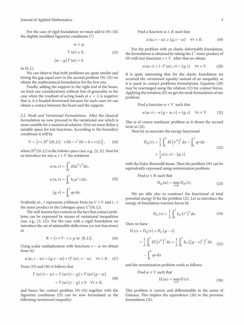
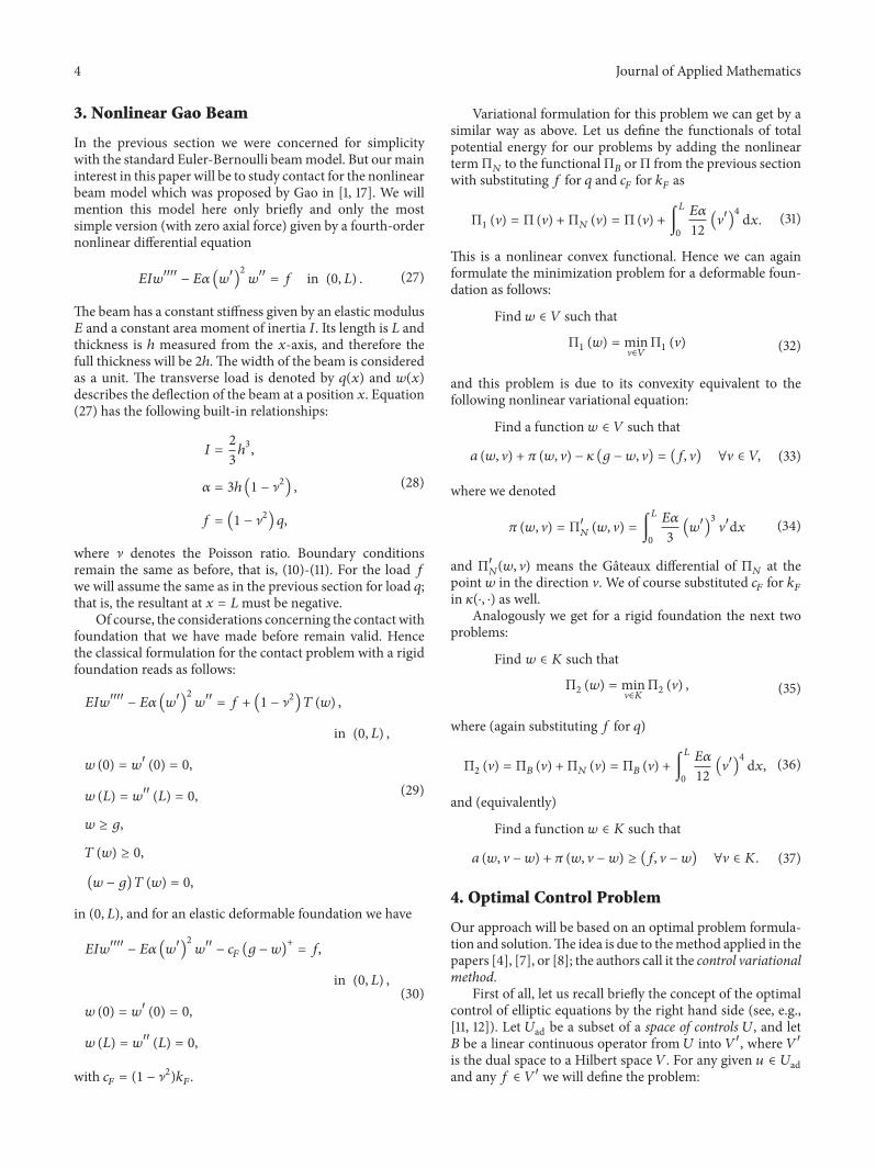
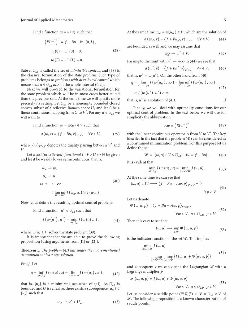
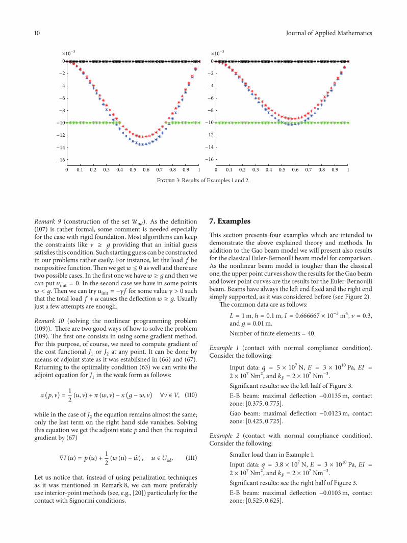
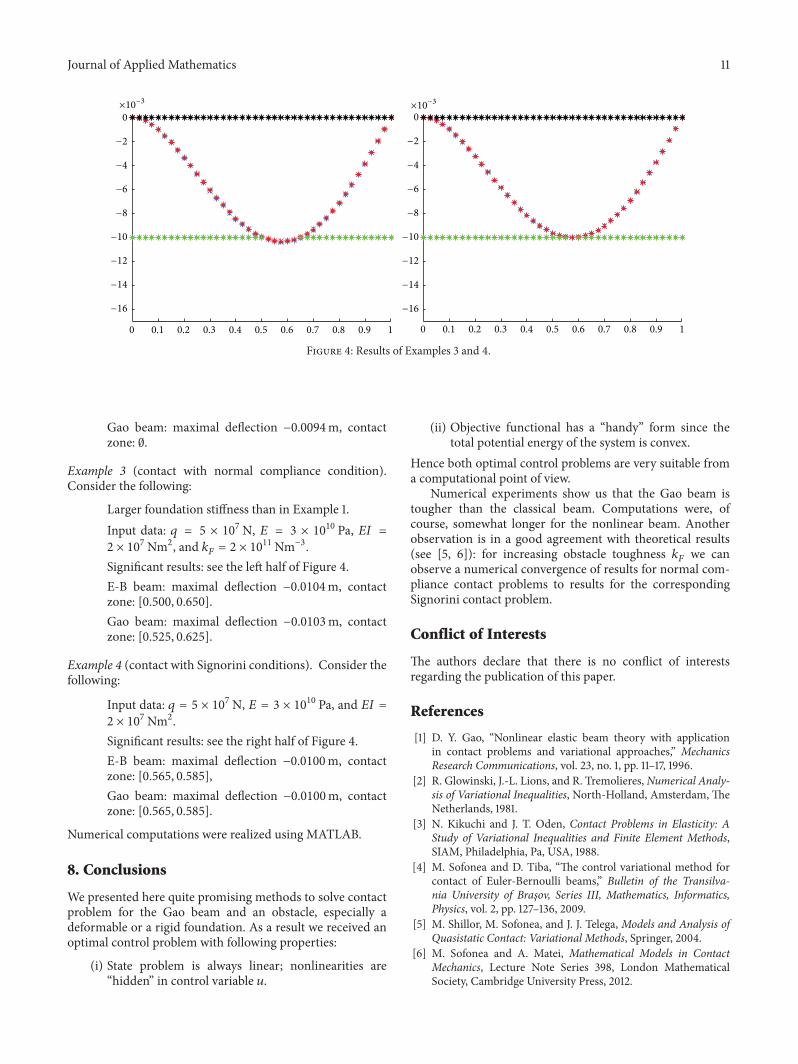