Embed Size (px)
Citation preview
Hindawi Publishing CorporationAdvances in Numerical AnalysisVolume 2013 Article ID 957496 8 pageshttpdxdoiorg1011552013957496
Research ArticleThree New Optimal Fourth-Order Iterative Methods toSolve Nonlinear Equations
Gustavo Fernaacutendez-Torres1 and Juan Vaacutesquez-Aquino2
1 Petroleum Engineering Department UNISTMO 70760 Tehuantepec OAX Mexico2 Applied Mathematics Department UNISTMO 70760 Tehuantepec OAX Mexico
Correspondence should be addressed to Gustavo Fernandez-Torres gusfersandungaunistmoedumx
Received 21 November 2012 Revised 24 January 2013 Accepted 2 February 2013
Academic Editor Michael Ng
Copyright copy 2013 G Fernandez-Torres and J Vasquez-Aquino This is an open access article distributed under the CreativeCommons Attribution License which permits unrestricted use distribution and reproduction in any medium provided theoriginal work is properly cited
We present new modifications to Newtonrsquos method for solving nonlinear equations The analysis of convergence shows that thesemethods have fourth-order convergence Each of the three methods uses three functional evaluations Thus according to Kung-Traubrsquos conjecture these are optimal methods With the previous ideas we extend the analysis to functions with multiple rootsSeveral numerical examples are given to illustrate that the presented methods have better performance compared with Newtonrsquosclassical method and other methods of fourth-order convergence recently published
1 Introduction
One of the most important problems in numerical analysisis solving nonlinear equations To solve these equations wecan use iterative methods such as Newtonrsquos method and itsvariants Newtonrsquos classical method for a single nonlinearequation 119891(119909) = 0 where 119903 is a single root is written as
119909119899+1
= 119909119899minus119891 (119909119899)
1198911015840 (119909119899) (1)
which converges quadratically in some neighborhood of 119903Taking 119910
119899= 119909119899minus 119891(119909
119899)1198911015840(119909
119899) many modifications of
Newtonrsquos method were recently published In [1] Noor andKhan presented a fourth-order optimal method as defined by
119909119899+1
= 119909119899minus119891 (119909119899) minus 119891 (119910
119899)
119891 (119909119899) minus 2119891 (119910
119899)
119891 (119909119899)
1198911015840 (119909119899) (2)
which uses three functional evaluations
In [2] Cordero et al proposed a fourth-order optimalmethod as defined by
119911119899= 119909119899minus119891 (119909119899) + 119891 (119910
119899)
1198911015840 (119909119899)
119908119899= 119911119899minus1198912 (119910119899) (2119891 (119909
119899) + 119891 (119910
119899))
1198912 (119909119899) 1198911015840 (119909
119899)
(3)
which also uses three functional evaluationsChun presented a third-order iterative formula [3] as
defined by
119909119899+1
= 119909119899minus3
2
119891 (119909119899)
1198911015840 (119909119899)+1
2
119891 (119909119899) 1198911015840 (120601 (119909
119899))
11989110158402 (119909119899)
(4)
which uses three functional evaluations where 120601 is anyiterative function of second order
2 Advances in Numerical Analysis
Li et al presented a fifth-order iterative formula in [4] asdefined by
119906119899+1
= 119909119899minus119891 (119909119899) minus 119891 (119909
119899minus 119891 (119909
119899) 1198911015840 (119909
119899))
1198911015840 (119909119899)
119909119899+1
= 119906119899+1
minus119891 (119906119899+1)
1198911015840 (119909119899minus 119891 (119909
119899) 1198911015840 (119909
119899))
(5)
which uses five functional evaluationsThe main goal and motivation in the development of
new methods are to obtain a better computational efficiencyIn other words it is advantageous to obtain the highestpossible convergence order with a fixed number of functionalevaluations per iteration In the case of multipoint methodswithout memory this demand is closely connected with theoptimal order considered in the Kung-Traubrsquos conjecture
Kung-Traubrsquos Conjecture (see [5]) Multipoint iterative meth-ods (without memory) requiring 119899+1 functional evaluationsper iteration have the order of convergence at most 2119899
Multipoint methods which satisfy Kung-Traubrsquos conjec-ture (still unproved) are usually called optimal methodsconsequently 119901 = 2119899 is the optimal order
The computational efficiency of an iterative method oforder 119901 requiring 119899 function evaluations per iteration ismost frequently calculated by Ostrowski-Traubrsquos efficiencyindex [6] 119864 = 1199011119899
On the case of multiple roots the quadratically conver-gent modified Newtonrsquos method [7] is
119909119899+1
= 119909119899minus119898119891 (119909
119899)
1198911015840 (119909119899) (6)
where119898 is the multiplicity of the rootFor this case there are severalmethods recently presented
to approximate the root of the function For example thecubically convergent Halleyrsquos method [8] is a special case ofthe Hansen-Patrickrsquos method [9]
119909119899+1
= 119909119899minus
119891 (119909119899)
((119898 + 1) 2119898)1198911015840 (119909119899) minus 119891 (119909
119899) 11989110158401015840 (119909
119899) 21198911015840 (119909
119899)
(7)
Osada [10] has developed a third-order method using thesecond derivative
119909119899+1
= 119909119899minus1
2119898 (119898 + 1) 119906
119899+1
2(119898 minus 1)
21198911015840 (119909119899)
11989110158401015840 (119909119899) (8)
where 119906119899= 119891(119909
119899)1198911015840(119909
119899)
Another third-order method [11] based on Kingrsquos fifth-order method (for simple roots) [12] is the Euler-Chebyshevrsquosmethod of order three
119909119899+1
= 119909119899minus119898 (3 minus 119898)
2
119891 (119909119899)
1198911015840 (119909119899)+1198982
2
1198912 (119909119899) 11989110158401015840 (119909
119899)
11989110158403 (119909119899)
(9)
Recently Chun and Neta [13] have developed a third-order method using the second derivative
119909119899+1
= 119909119899minus (211989821198912 (119909
119899) 11989110158401015840 (119909
119899)
times (119898 (3 minus 119898)119891 (119909119899) 1198911015840 (119909
119899) 11989110158401015840 (119909
119899)
+(119898 minus 1)211989110158403 (119909
119899))minus1
)
(10)
All previous methods use the second derivative of thefunction to obtain a greater order of convergence Theobjective of the new method is to avoid the use of the secondderivative
The new methods are based on a mixture of LagrangersquosandHermitersquos interpolationsThat is to say not only Hermitersquosinterpolation This is the novelty of the new methods Theinterpolation process is a conventional tool for iterativemethods see [5 7] However this tool has been appliedrecently in several ways For example in [14] Cordero andTorregrosa presented a family of Steffensen-type methodsof fourth-order convergence for solving nonlinear smoothequations by using a linear combination of divided differ-ences to achieve a better approximation to the derivativeZheng et al [15] proposed a general family of Steffensen-type methods with optimal order of convergence by usingNewtonrsquos iteration for the direct Newtonian interpolation In[16] Petkovic et al investigated a general way to constructmultipoint methods for solving nonlinear equations by usinginverse interpolation In [17] Dzunic et al presented anew family of three-point derivative free methods by usinga self-correcting parameter that is calculated applying thesecant-type method in three different ways and Newtonrsquosinterpolatory polynomial of the second degree
The three new methods (for simple roots) in this paperuse three functional evaluations and have fourth-order con-vergence thus they are optimal methods and their efficiencyindex is 119864 = 1587 which is greater than the efficiencyindex of Newtonrsquos method which is 119864 = 1414 In the caseof multiple roots the method developed here is cubicallyconvergent and uses three functional evaluations without theuse of second derivative of the functionThus themethod hasbetter performance than Newtonrsquos modified method and theabove methods with efficiency index 119864 = 14422
2 Development of the Methods
In this paper we consider iterative methods to find a simpleroot 119903 isin 119868 of a nonlinear equation 119891(119909) = 0 where 119891 119868 rarrR is a scalar function for an open interval 119868 We suppose that119891(119909) is sufficiently differentiable and 1198911015840(119909) = 0 for 119909 isin 119868 andsince 119903 is a simple root we can define 119892 = 119891minus1 on 119868 Taking1199090isin 119868 closer to 119903 and supposing that 119909
119899has been chosen we
define
119911119899= 119909119899minus119891 (119909119899)
1198911015840 (119909119899)
119870 = 119891 (119909119899) 119871 = 119891 (119911
119899)
(11)
Advances in Numerical Analysis 3
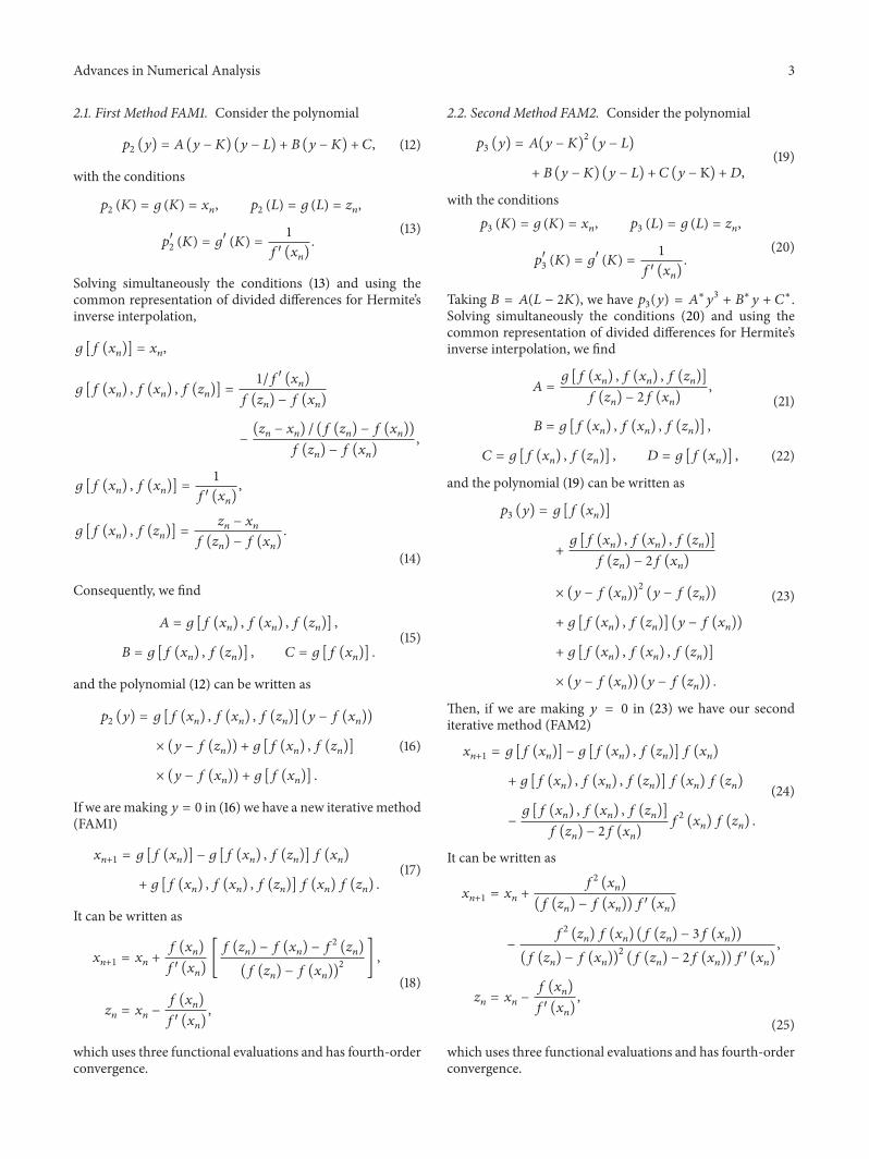
21 First Method FAM1 Consider the polynomial
1199012(119910) = 119860 (119910 minus 119870) (119910 minus 119871) + 119861 (119910 minus 119870) + 119862 (12)
with the conditions
1199012(119870) = 119892 (119870) = 119909
119899 119901
2(119871) = 119892 (119871) = 119911
119899
11990110158402(119870) = 119892
1015840
(119870) =1
1198911015840 (119909119899)
(13)
Solving simultaneously the conditions (13) and using thecommon representation of divided differences for Hermitersquosinverse interpolation
119892 [119891 (119909119899)] = 119909
119899
119892 [119891 (119909119899) 119891 (119909
119899) 119891 (119911
119899)] =
11198911015840 (119909119899)
119891 (119911119899) minus 119891 (119909
119899)
minus(119911119899minus 119909119899) (119891 (119911
119899) minus 119891 (119909
119899))
119891 (119911119899) minus 119891 (119909
119899)
119892 [119891 (119909119899) 119891 (119909
119899)] =
1
1198911015840 (119909119899)
119892 [119891 (119909119899) 119891 (119911
119899)] =
119911119899minus 119909119899
119891 (119911119899) minus 119891 (119909
119899)
(14)
Consequently we find
119860 = 119892 [119891 (119909119899) 119891 (119909
119899) 119891 (119911
119899)]
119861 = 119892 [119891 (119909119899) 119891 (119911
119899)] 119862 = 119892 [119891 (119909
119899)]
(15)
and the polynomial (12) can be written as
1199012(119910) = 119892 [119891 (119909
119899) 119891 (119909
119899) 119891 (119911
119899)] (119910 minus 119891 (119909
119899))
times (119910 minus 119891 (119911119899)) + 119892 [119891 (119909
119899) 119891 (119911
119899)]
times (119910 minus 119891 (119909119899)) + 119892 [119891 (119909
119899)]
(16)
If we aremaking 119910 = 0 in (16) we have a new iterativemethod(FAM1)
119909119899+1
= 119892 [119891 (119909119899)] minus 119892 [119891 (119909
119899) 119891 (119911
119899)] 119891 (119909
119899)
+ 119892 [119891 (119909119899) 119891 (119909
119899) 119891 (119911
119899)] 119891 (119909
119899) 119891 (119911119899)
(17)
It can be written as
119909119899+1
= 119909119899+119891 (119909119899)
1198911015840 (119909119899)[119891 (119911119899) minus 119891 (119909
119899) minus 1198912 (119911
119899)
(119891 (119911119899) minus 119891 (119909
119899))2
]
119911119899= 119909119899minus119891 (119909119899)
1198911015840 (119909119899)
(18)
which uses three functional evaluations and has fourth-orderconvergence
22 Second Method FAM2 Consider the polynomial
1199013(119910) = 119860(119910 minus 119870)
2
(119910 minus 119871)
+ 119861 (119910 minus 119870) (119910 minus 119871) + 119862 (119910 minus K) + 119863(19)
with the conditions1199013(119870) = 119892 (119870) = 119909
119899 119901
3(119871) = 119892 (119871) = 119911
119899
11990110158403(119870) = 119892
1015840
(119870) =1
1198911015840 (119909119899)
(20)
Taking 119861 = 119860(119871 minus 2119870) we have 1199013(119910) = 119860lowast1199103 + 119861lowast119910 + 119862lowast
Solving simultaneously the conditions (20) and using thecommon representation of divided differences for Hermitersquosinverse interpolation we find
119860 =119892 [119891 (119909
119899) 119891 (119909
119899) 119891 (119911
119899)]
119891 (119911119899) minus 2119891 (119909
119899)
119861 = 119892 [119891 (119909119899) 119891 (119909
119899) 119891 (119911
119899)]
(21)
119862 = 119892 [119891 (119909119899) 119891 (119911
119899)] 119863 = 119892 [119891 (119909
119899)] (22)
and the polynomial (19) can be written as
1199013(119910) = 119892 [119891 (119909
119899)]
+119892 [119891 (119909
119899) 119891 (119909
119899) 119891 (119911
119899)]
119891 (119911119899) minus 2119891 (119909
119899)
times (119910 minus 119891 (119909119899))2
(119910 minus 119891 (119911119899))
+ 119892 [119891 (119909119899) 119891 (119911
119899)] (119910 minus 119891 (119909
119899))
+ 119892 [119891 (119909119899) 119891 (119909
119899) 119891 (119911
119899)]
times (119910 minus 119891 (119909119899)) (119910 minus 119891 (119911
119899))
(23)
Then if we are making 119910 = 0 in (23) we have our seconditerative method (FAM2)
119909119899+1
= 119892 [119891 (119909119899)] minus 119892 [119891 (119909
119899) 119891 (119911
119899)] 119891 (119909
119899)
+ 119892 [119891 (119909119899) 119891 (119909
119899) 119891 (119911
119899)] 119891 (119909
119899) 119891 (119911119899)
minus119892 [119891 (119909
119899) 119891 (119909
119899) 119891 (119911
119899)]
119891 (119911119899) minus 2119891 (119909
119899)
1198912 (119909119899) 119891 (119911119899)
(24)
It can be written as
119909119899+1
= 119909119899+
1198912 (119909119899)
(119891 (119911119899) minus 119891 (119909
119899)) 1198911015840 (119909
119899)
minus1198912 (119911119899) 119891 (119909
119899) (119891 (119911
119899) minus 3119891 (119909
119899))
(119891 (119911119899) minus 119891 (119909
119899))2
(119891 (119911119899) minus 2119891 (119909
119899)) 1198911015840 (119909
119899)
119911119899= 119909119899minus119891 (119909119899)
1198911015840 (119909119899)
(25)
which uses three functional evaluations and has fourth-orderconvergence
4 Advances in Numerical Analysis
23 Third Method FAM3 Consider the polynomial
1199013(119910) = 119860(119910 minus 119870)
2
(119910 minus 119871)
+ 119861 (119910 minus 119870) (119910 minus 119871) + 119862 (119910 minus 119870) + 119863(26)
with the conditions
1199013(119870) = 119892 (119870) = 119909
119899 119901
3(119871) = 119892 (119871) = 119911
119899
11990110158403(119870) = 119892
1015840
(119870) =1
1198911015840 (119909119899)
(27)
119901101584010158403(119870) = minus
2119891 (119911119899)
1198912 (119909119899) 1198911015840 (119909
119899) (28)
where we have used an approximation of 11989110158401015840(119909119899) in [2]
11989110158401015840(119909119899) asymp 2119891(119911
119899)11989110158402(119909
119899)1198912(119909
119899) Solving simultaneously the
conditions (27) and (28) and using the common representa-tion of divided differences forHermitersquos inverse interpolationwe have
119860 = (119892 [119891 (119909119899) 119891 (119909
119899)]
119891 (119911119899)
1198912 (119909119899)
+119892 [119891 (119909119899) 119891 (119909
119899) 119891 (119911
119899)] )
times (119891 (119911119899) minus 119891 (119909
119899))minus1
(29)
119861 = 119892 [119891 (119909119899) 119891 (119909
119899) 119891 (119911
119899)]
119862 = 119892 [119891 (119909119899) 119891 (119911
119899)] 119863 = 119892 [119891 (119909
119899)]
(30)
Thus the polynomial (26) can be written as
1199013(119910) = (
119892 [119891 (119909119899) 119891 (119909
119899)] (119891 (119911
119899) 1198912 (119909
119899))
119891 (119911119899) minus 119891 (119909
119899)
+119892 [119891 (119909
119899) 119891 (119909
119899) 119891 (119911
119899)]
119891 (119911119899) minus 119891 (119909
119899)
)
times (119910 minus 119891 (119909119899))2
(119910 minus 119891 (119911119899))
+ 119892 [119891 (119909119899) 119891 (119909
119899) 119891 (119911
119899)]
times (119910 minus 119891 (119909119899)) (119910 minus 119891 (119911
119899))
+ 119892 [119891 (119909119899) 119891 (119911
119899)] (119910 minus 119891 (119909
119899)) + 119892 [119891 (119909
119899)]
(31)
Making 119910 = 0 in (31) we have
119909119899+1
= 119892 [119891 (119909119899)] minus 119892 [119891 (119909
119899) 119891 (119911
119899)] 119891 (119909
119899)
+ 119892 [119891 (119909119899) 119891 (119909
119899) 119891 (119911
119899)] 119891 (119909
119899) 119891 (119911119899)
minus (119892 [119891 (119909
119899) 119891 (119909
119899)] (119891 (119911
119899) 1198912 (119909
119899))
119891 (119911119899) minus 119891 (119909
119899)
+119892 [119891 (119909
119899) 119891 (119909
119899) 119891 (119911
119899)]
119891 (119911119899) minus 119891 (119909
119899)
)
times 1198912 (119909119899) 119891 (119911119899)
(32)
It can be written as
119909119899+1
= 119909119899+119891 (119911119899) 119891 (119909
119899) minus 1198912 (119909
119899) minus 1198912 (119911
119899)
(119891 (119911119899) minus 119891 (119909
119899))2
119891 (119909119899)
1198911015840 (119909119899)
minus1198913 (119911119899) (119891 (119911
119899) minus 2119891 (119909
119899))
(119891 (119911119899) minus 119891 (119909
119899))3
1198912 (119909119899)
1198911015840 (119909119899)
119911119899= 119909119899minus119891 (119909119899)
1198911015840 (119909119899)
(33)
which uses three functional evaluations and has fourth-orderconvergence
24 Method FAM4 (Multiple Roots) Consider the polyno-mial
119901119898(119909) = 119860(119909 minus 119909
119899+ 119908)119898
(34)
where 119898 is the multiplicity of the root and 119901119898(119909) verify the
conditions
119901119898(119909119899) = 119891 (119909
119899) 119901
119898(119911119899) = 119891 (119911
119899) (35)
with 119911119899= 119909119899minus 119898(119891(119909
119899)1198911015840(119909
119899))
Solving the system we obtain
119908 =119906119898(119911119899minus 119909119899)
1 minus 119906119898
(36)
where
119906119898= [
119891 (119909119899)
119891 (119910119899)]
1119898
(37)
Thus we have
119909119899+1
= 119909119899minus 119908 (38)
that can be written as
119909119899+1
= 119911119899+119898119891 (119909
119899)
1198911015840 (119909119899)
1
1 minus 119906119898
119911119899= 119909119899minus 119898
119891 (119909119899)
1198911015840 (119909119899) 119906
119898= [
119891 (119909119899)
119891 (119910119899)]
1119898
(39)
which uses three functional evaluations and has third-orderconvergence
Advances in Numerical Analysis 5
3 Analysis of Convergence
Theorem 1 Let 119891 119868subeR rarr R be a sufficiently differentiablefunction and let 119903 isin 119868 be a simple zero of 119891(119909) = 0 in an openinterval 119868 with 1198911015840(119909) = 0 on 119868 If 119909
0isin 119868 is sufficiently close to 119903
then the methods FAM1 FAM2 and FAM3 as defined by (18)(25) and (33) have fourth-order convergence
Proof Following an analogous procedure to find the errorin Lagrangersquos and Hermitersquos interpolations the polynomials(12) (19) and (26) in FAM1 FAM2 and FAM3 respectivelyhave the error
119864 (119910) = 119892 (119910) minus 119901119899(119910) = [
119892101584010158401015840 (120585)
3minus 120573119860] (119910 minus 119870)
2
(119910 minus 119871)
(40)
for some 120585 isin 119868 119860 is the coefficient in (15) (21) (29)that appears in the polynomial 119901
119899(119910) in (12) (19) and (26)
respectivelyThen substituting 119910 = 0 in 119864(119910)
119903 minus 119909119899+1
= minus [119892101584010158401015840 (120585)
3minus 120573119860]1198702119871
= minus [119892101584010158401015840 (120585)
3minus 120573119860]1198912 (119909
119899) 119891 (119911119899)
119909119899+1
minus 119903 = [119892101584010158401015840 (120585)
3minus 120573119860]
times [119891 (119903) + 1198911015840 (1205851) (119909119899minus 119903)]2
times [119891 (119903) + 1198911015840 (1205852) (119911119899minus 119903)]
(41)
with 119909119899+1
minus 119903 = 120598119899+1 119909119899minus 119903 = 120598
119899 Since 119911
119899was taken from
Newtonrsquosmethod we know that 119911119899minus119903 = (11989110158401015840(120585
3)21198911015840(120585
4))1205852119899+
119874(1205852119899+1) Then we have
120598119899+1
asymp [119892101584010158401015840 (120585)
3minus 120573119860]
11989110158402 (1205851) 12058521198991198911015840 (1205852) 11989110158401015840 (120585
3) 1205852119899
21198911015840 (1205854)
120598119899+1
asymp [119892101584010158401015840 (120585)
3minus 120573119860]
11989110158402 (1205851) 1198911015840 (120585
2) 11989110158401015840 (120585
3)
21198911015840 (1205854)
1205854119899
(42)
Now in FAM1 we take 120573 = 0 then
120585119899+1
asymp119892101584010158401015840 (120585)
3
11989110158402 (1205851) 1198911015840 (120585
2) 11989110158401015840 (120585
3)
21198911015840 (1205854)
1205854119899 (43)
In FAM2 and FAM3 we take 120573 = 1 then
120585119899+1
asymp [119892101584010158401015840 (120585)
3minus 119860]
11989110158402 (1205851) 1198911015840 (120585
2) 11989110158401015840 (120585
3)
21198911015840 (1205854)
1205854119899
120585119899+1
1205854119899
asymp [119892101584010158401015840 (120585)
3minus 119860]
11989110158402 (1205851) 1198911015840 (120585
2) 11989110158401015840 (120585
3)
21198911015840 (1205854)
(44)
Thus FAM1 FAM2 and FAM3 have fourth-order conver-gence
Theorem 2 Let 119891 119868 sube R rarr R be a sufficientlydifferentiable function and let 119903 isin 119868 be a zero of 119891(119909) = 0 withmultiplicity119898 in an open interval 119868 If 119909
0isin 119868 is sufficiently close
to 119903 then the method FAM4 defined by (12) (20) is cubicallyconvergent
Proof The proof is based on the error of Lagrangersquos interpo-lation Suppose that 119909
119899has been chosen We can see that
119891 (119909) minus 119901119898(119909) =
11989110158401015840 (1205851) minus 11990110158401015840119898(1205851)
2(119909 minus 119909
119899) (119909 minus 119911
119899) (45)
for some 1205851isin 119868
Taking 119909 = 119903 and expanding 119901119898(119903) around 119909
119896+1 we have
minus1199011015840119898(1205852) (119903 minus 119909
119899+1) =
11989110158401015840 (1205851) minus 11990110158401015840119898(1205851)
2(119903 minus 119909
119899) (119903 minus 119911
119899)
(46)
with 1205851 1205852isin 119868
Since 119911119899= 119909119899minus 119898(119891(119909
119899)1198911015840(119909
119899)) we know that
119911119899minus 119903 =
11989110158401015840 (1205853) minus 11990110158401015840119898(1205853)
21199011015840119898(1205854)
1205982119899 (47)
for some 1205853 1205854isin 119868
Thus
120598119899+1
=11989110158401015840 (1205851) minus 11990110158401015840119898(1205851)
21199011015840119898(1205852)
11989110158401015840 (1205853) minus 11990110158401015840119898(1205853)
21199011015840 (1205854)
1205983119899 (48)
Therefore FAM4 has third-order convergence
Note that 11990110158401015840119898is not zero for119898 ge 2 and this fact allows the
convergence of lim119899rarrinfin
(120598119899+11205983119899)
4 Numerical Analysis
In this section we use numerical examples to comparethe new methods introduced in this paper with Newtonrsquosclassical method (NM) and recent methods of fourth-orderconvergence such as Noorrsquos method (NOM) with 119864 = 1587in [1] Corderorsquos method (CM) with 119864 = 1587 in [2] Chunrsquosthird-order method (CHM) with 119864 = 1442 in [3] andLirsquos fifth-order method (ZM) with 119864 = 1379 in [4] in thecase of simple roots For multiple roots we compare themethod developed here with the quadratically convergentNewtonrsquos modified method (NMM) and with the cubicallyconvergent Halleyrsquos method (HM) Osadarsquos method (OM)Euler-Chebyshevrsquos method (ECM) and Chun-Netarsquos method(CNM) Tables 2 and 4 show the number of iterations (IT) andthe number of functional evaluations (NOFE) The resultsobtained show that the methods presented in this paper aremore efficient
All computations were done using MATLAB 2010 Weaccept an approximate solution rather than the exact rootdepending on the precision (120598) of the computer We use
6 Advances in Numerical Analysis
Table 1 List of functions for a single root
1198911(119909) = 1199093 + 41199092 minus 10 119903 = 13652300134140968457608068290
1198912(119909) = cos(119909) minus 119909 119903 = 073908513321516064165531208767
1198913(119909) = sin(119909) minus (12) 119909 119903 = 18954942670339809471440357381
1198914(119909) = sin2(119909) minus 1199092 + 1 119903 = 14044916482153412260350868178
1198915(119909) = 119909119890119909
2
minus sin2(119909) + 3 cos(119909) + 5 119903 = 12076478271309189270094167584
1198916(119909) = 1199092 minus 119890119909 minus 3119909 + 2 119903 = 0257530285439860760455367304944
1198917(119909) = (119909 minus 1)3 minus 2 119903 = 22599210498948731647672106073
1198918(119909) = (119909 minus 1)2 minus 1 119903 = 2
1198919(119909) = 10119909119890minus119909
2
minus 1 119903 = 16796306104284499
11989110(119909) = (119909 + 2)119890119909 minus 1 119903 = minus04428544010023885831413280000
11989111(119909) = 119890minus119909 + cos(119909) 119903 = 1746139530408012417650703089
Table 2 Comparison of the methods for a single root
119891(119909) 1199090
IT NOFE
NM NOM CHM CM ZM FAM1 FAM2 FAM3 NM NOM CHM CM ZM FAM1 FAM2 FAM3
1198911(119909) 1 6 4 5 4 4 3 3 3 12 12 15 12 12 9 9 9
1198912(119909) 1 5 3 4 2 3 3 3 2 10 9 12 6 9 9 9 6
1198913(119909) 2 5 2 4 3 3 2 3 2 10 6 12 9 9 6 9 6
1198914(119909) 13 5 3 4 4 3 3 3 2 10 9 12 12 9 9 9 6
1198915(119909) -1 6 4 5 4 4 4 4 3 12 12 15 12 12 12 12 9
1198916(119909) 2 6 4 5 4 4 3 4 3 12 12 15 12 12 9 12 9
1198917(119909) 3 7 4 5 4 4 4 3 3 14 12 15 12 12 12 9 9
1198918(119909) 35 6 3 5 3 4 3 3 3 12 9 15 9 12 9 9 9
1198919(119909) 1 6 4 6 4 4 3 3 3 12 12 18 12 12 9 9 9
11989110(119909) 2 9 5 7 6 5 4 4 4 18 15 21 18 15 12 12 12
11989111(119909) 05 5 4 4 4 3 3 3 3 10 12 12 12 9 9 9 9
the following stopping criteria for computer programs (i)|119909119899+1
minus 119909119899| lt 120598 (ii) |119891(119909
119899+1)| lt 120598 Thus when the stopping
criterion is satisfied 119909119899+1
is taken as the exact computed root119903 For numerical illustrations in this section we used the fixedstopping criterion 120598 = 10minus18
We used the functions in Tables 1 and 3The computational results presented in Tables 2 and 4
show that in almost all of cases the presented methodsconverge more rapidly than Newtonrsquos method Newtonrsquosmodified method and those previously presented for thecase of simple and multiple roots The new methods requireless number of functional evaluations This means that thenew methods have better efficiency in computing processthan Newtonrsquos method as compared to other methods and
furthermore themethod FAM3produces the best results Formost of the functions we tested the obtainedmethods behaveat least with equal performance compared to the other knownmethods of the same order
5 Conclusions
In this paper we introduce three new optimal fourth-order iterative methods to solve nonlinear equations Theanalysis of convergence shows that the three new methodshave fourth-order convergence they use three functionalevaluations and thus according to Kung-Traubrsquos conjecturethey are optimal methods In the case of multiple roots themethod developed here is cubically convergent and uses three
Advances in Numerical Analysis 7
Table 3 List of functions for a multiple root
1198911(119909) = (1199093 + 41199092 minus 10)3 119903 = 13652300134140968457608068290
1198912(119909) = (sin2(119909) minus 1199092 + 1)2 119903 = 14044916482153412260350868178
1198913(119909) = (1199092 minus 119890119909 minus 3119909 + 2)5 119903 = 02575302854398607604553673049
1198914(119909) = (cos(119909) minus 119909)3 119903 = 07390851332151606416553120876
1198915(119909) = ((119909 minus 1)3 minus 1)6 119903 = 2
1198916(119909) = (119909119890119909
2
minus sin2(119909) + 3 cos(119909) + 5)4 119903 = minus12076478271309189270094167581198917(119909) = (sin(119909) minus (12) 119909)2 119903 = 18954942670339809471440357381
Table 4 Comparison of the methods for a multiple root
119891(119909) 1199090
IT NOFENMM HM OM ECM CNM FAM4 NMM HM OM ECM CNM FAM4
2 5 3 3 3 3 3 10 9 9 9 9 91198911(119909) 1 5 3 4 3 3 3 10 9 12 9 9 9
minus03 54 5 5 5 5 4 108 15 15 15 15 1223 6 4 4 4 4 4 12 12 12 12 12 12
1198912(119909) 2 6 4 4 4 4 4 12 12 12 12 12 12
15 5 4 4 4 3 3 10 12 12 12 9 90 4 3 3 3 3 2 8 9 9 9 9 6
1198913(119909) 1 4 4 4 4 4 3 8 12 12 12 12 9
minus1 5 4 4 4 4 3 10 12 12 12 12 917 5 4 4 4 4 3 10 12 12 12 12 9
1198914(119909) 1 4 3 3 3 3 3 8 9 9 9 9 9
minus3 99 8 8 8 8 7 198 24 24 24 24 213 6 4 5 5 4 4 12 12 15 15 12 12
1198915(119909) minus1 10 11 24 23 5 6 20 33 72 79 15 18
5 8 9 15 15 5 5 16 27 45 45 15 15minus2 8 5 6 6 6 5 16 15 18 18 18 15
1198916(119909) minus1 5 3 4 3 3 5 10 9 12 9 9 15
minus3 14 9 10 10 10 9 28 27 30 30 30 2717 5 3 4 3 4 4 10 9 12 9 12 12
1198917(119909) 2 4 3 3 3 3 3 8 9 9 9 9 9
3 5 3 3 3 3 3 10 9 9 9 9 9
functional evaluations without the use of second derivativeNumerical analysis shows that these methods have betterperformance as compared with Newtonrsquos classical methodNewtonrsquos modified method and other recent methods ofthird- (multiple roots) and fourth-order (simple roots) con-vergence
Acknowledgments
The authors wishes to acknowledge the valuable participa-tion of Professor Nicole Mercier and Professor Joelle AnnLabrecque in the proofreading of this paper This paperis the result of the research project ldquoAnalisis Numerico deMetodos Iterativos Optimos para la Solucion de EcuacionesNoLinealesrdquo developed at theUniversidad del IstmoCampus
Tehuantepec by Researcher-Professor Gustavo Fernandez-Torres
References
[1] M A Noor and W A Khan ldquoFourth-order iterative methodfree from second derivative for solving nonlinear equationsrdquoAppliedMathematical Sciences vol 6 no 93ndash96 pp 4617ndash46252012
[2] A Cordero J L Hueso E Martınez and J R Torregrosa ldquoNewmodifications of Potra-Ptakrsquos method with optimal fourth andeighth orders of convergencerdquo Journal of Computational andApplied Mathematics vol 234 no 10 pp 2969ndash2976 2010
[3] C Chun ldquoA geometric construction of iterative formulas oforder threerdquoAppliedMathematics Letters vol 23 no 5 pp 512ndash516 2010
8 Advances in Numerical Analysis
[4] Z Li C Peng T Zhou and J Gao ldquoA new Newton-typemethod for solving nonlinear equations with any integer orderof convergencerdquo Journal of Computational Information Systemsvol 7 no 7 pp 2371ndash2378 2011
[5] H T Kung and J F Traub ldquoOptimal order of one-point andmultipoint iterationrdquo Journal of the Association for ComputingMachinery vol 21 pp 643ndash651 1974
[6] A M Ostrowski Solution of Equations and Systems of Equa-tions Academic Press New York NY USA 1966
[7] A Ralston and P Rabinowitz A First Course in NumericalAnalysis McGraw-Hill 1978
[8] E Halley ldquoA new exact and easy method of finding the roots ofequations generally and that without any previous reductionrdquoPhilosophical Transactions of the Royal Society of London vol18 pp 136ndash148 1964
[9] E Hansen and M Patrick ldquoA family of root finding methodsrdquoNumerische Mathematik vol 27 no 3 pp 257ndash269 1977
[10] N Osada ldquoAn optimal multiple root-finding method of orderthreerdquo Journal of Computational and Applied Mathematics vol51 no 1 pp 131ndash133 1994
[11] H D Victory and B Neta ldquoA higher order method for multiplezeros of nonlinear functionsrdquo International Journal of ComputerMathematics vol 12 no 3-4 pp 329ndash335 1983
[12] R F King ldquoA family of fourth order methods for nonlinearequationsrdquo SIAM Journal on Numerical Analysis vol 10 pp876ndash879 1973
[13] C Chun and B Neta ldquoA third-order modification of Newtonrsquosmethod for multiple rootsrdquoAppliedMathematics and Computa-tion vol 211 no 2 pp 474ndash479 2009
[14] A Cordero and J R Torregrosa ldquoA class of Steffensen typemethods with optimal order of convergencerdquo Applied Mathe-matics and Computation vol 217 no 19 pp 7653ndash7659 2011
[15] Q Zheng J Li and F Huang ldquoAn optimal Steffensen-typefamily for solving nonlinear equationsrdquo Applied Mathematicsand Computation vol 217 no 23 pp 9592ndash9597 2011
[16] M S Petkovic J Dzunic and B Neta ldquoInterpolatory multi-point methods with memory for solving nonlinear equationsrdquoAppliedMathematics and Computation vol 218 no 6 pp 2533ndash2541 2011
[17] J Dzunic M S Petkovic and L D Petkovic ldquoThree-pointmethods with and without memory for solving nonlinearequationsrdquo Applied Mathematics and Computation vol 218 no9 pp 4917ndash4927 2012
Submit your manuscripts athttpwwwhindawicom
Hindawi Publishing Corporationhttpwwwhindawicom Volume 2014
MathematicsJournal of
Hindawi Publishing Corporationhttpwwwhindawicom Volume 2014
Mathematical Problems in Engineering
Hindawi Publishing Corporationhttpwwwhindawicom
Differential EquationsInternational Journal of
Volume 2014
Applied MathematicsJournal of
Hindawi Publishing Corporationhttpwwwhindawicom Volume 2014
Probability and StatisticsHindawi Publishing Corporationhttpwwwhindawicom Volume 2014
Journal of
Hindawi Publishing Corporationhttpwwwhindawicom Volume 2014
Mathematical PhysicsAdvances in
Complex AnalysisJournal of
Hindawi Publishing Corporationhttpwwwhindawicom Volume 2014
OptimizationJournal of
Hindawi Publishing Corporationhttpwwwhindawicom Volume 2014
CombinatoricsHindawi Publishing Corporationhttpwwwhindawicom Volume 2014
International Journal of
Hindawi Publishing Corporationhttpwwwhindawicom Volume 2014
Operations ResearchAdvances in
Journal of
Hindawi Publishing Corporationhttpwwwhindawicom Volume 2014
Function Spaces
Abstract and Applied AnalysisHindawi Publishing Corporationhttpwwwhindawicom Volume 2014
International Journal of Mathematics and Mathematical Sciences
Hindawi Publishing Corporationhttpwwwhindawicom Volume 2014
The Scientific World JournalHindawi Publishing Corporation httpwwwhindawicom Volume 2014
Hindawi Publishing Corporationhttpwwwhindawicom Volume 2014
Algebra
Discrete Dynamics in Nature and Society
Hindawi Publishing Corporationhttpwwwhindawicom Volume 2014
Hindawi Publishing Corporationhttpwwwhindawicom Volume 2014
Decision SciencesAdvances in
Discrete MathematicsJournal of
Hindawi Publishing Corporationhttpwwwhindawicom
Volume 2014 Hindawi Publishing Corporationhttpwwwhindawicom Volume 2014
Stochastic AnalysisInternational Journal of
2 Advances in Numerical Analysis
Li et al presented a fifth-order iterative formula in [4] asdefined by
119906119899+1
= 119909119899minus119891 (119909119899) minus 119891 (119909
119899minus 119891 (119909
119899) 1198911015840 (119909
119899))
1198911015840 (119909119899)
119909119899+1
= 119906119899+1
minus119891 (119906119899+1)
1198911015840 (119909119899minus 119891 (119909
119899) 1198911015840 (119909
119899))
(5)
which uses five functional evaluationsThe main goal and motivation in the development of
new methods are to obtain a better computational efficiencyIn other words it is advantageous to obtain the highestpossible convergence order with a fixed number of functionalevaluations per iteration In the case of multipoint methodswithout memory this demand is closely connected with theoptimal order considered in the Kung-Traubrsquos conjecture
Kung-Traubrsquos Conjecture (see [5]) Multipoint iterative meth-ods (without memory) requiring 119899+1 functional evaluationsper iteration have the order of convergence at most 2119899
Multipoint methods which satisfy Kung-Traubrsquos conjec-ture (still unproved) are usually called optimal methodsconsequently 119901 = 2119899 is the optimal order
The computational efficiency of an iterative method oforder 119901 requiring 119899 function evaluations per iteration ismost frequently calculated by Ostrowski-Traubrsquos efficiencyindex [6] 119864 = 1199011119899
On the case of multiple roots the quadratically conver-gent modified Newtonrsquos method [7] is
119909119899+1
= 119909119899minus119898119891 (119909
119899)
1198911015840 (119909119899) (6)
where119898 is the multiplicity of the rootFor this case there are severalmethods recently presented
to approximate the root of the function For example thecubically convergent Halleyrsquos method [8] is a special case ofthe Hansen-Patrickrsquos method [9]
119909119899+1
= 119909119899minus
119891 (119909119899)
((119898 + 1) 2119898)1198911015840 (119909119899) minus 119891 (119909
119899) 11989110158401015840 (119909
119899) 21198911015840 (119909
119899)
(7)
Osada [10] has developed a third-order method using thesecond derivative
119909119899+1
= 119909119899minus1
2119898 (119898 + 1) 119906
119899+1
2(119898 minus 1)
21198911015840 (119909119899)
11989110158401015840 (119909119899) (8)
where 119906119899= 119891(119909
119899)1198911015840(119909
119899)
Another third-order method [11] based on Kingrsquos fifth-order method (for simple roots) [12] is the Euler-Chebyshevrsquosmethod of order three
119909119899+1
= 119909119899minus119898 (3 minus 119898)
2
119891 (119909119899)
1198911015840 (119909119899)+1198982
2
1198912 (119909119899) 11989110158401015840 (119909
119899)
11989110158403 (119909119899)
(9)
Recently Chun and Neta [13] have developed a third-order method using the second derivative
119909119899+1
= 119909119899minus (211989821198912 (119909
119899) 11989110158401015840 (119909
119899)
times (119898 (3 minus 119898)119891 (119909119899) 1198911015840 (119909
119899) 11989110158401015840 (119909
119899)
+(119898 minus 1)211989110158403 (119909
119899))minus1
)
(10)
All previous methods use the second derivative of thefunction to obtain a greater order of convergence Theobjective of the new method is to avoid the use of the secondderivative
The new methods are based on a mixture of LagrangersquosandHermitersquos interpolationsThat is to say not only Hermitersquosinterpolation This is the novelty of the new methods Theinterpolation process is a conventional tool for iterativemethods see [5 7] However this tool has been appliedrecently in several ways For example in [14] Cordero andTorregrosa presented a family of Steffensen-type methodsof fourth-order convergence for solving nonlinear smoothequations by using a linear combination of divided differ-ences to achieve a better approximation to the derivativeZheng et al [15] proposed a general family of Steffensen-type methods with optimal order of convergence by usingNewtonrsquos iteration for the direct Newtonian interpolation In[16] Petkovic et al investigated a general way to constructmultipoint methods for solving nonlinear equations by usinginverse interpolation In [17] Dzunic et al presented anew family of three-point derivative free methods by usinga self-correcting parameter that is calculated applying thesecant-type method in three different ways and Newtonrsquosinterpolatory polynomial of the second degree
The three new methods (for simple roots) in this paperuse three functional evaluations and have fourth-order con-vergence thus they are optimal methods and their efficiencyindex is 119864 = 1587 which is greater than the efficiencyindex of Newtonrsquos method which is 119864 = 1414 In the caseof multiple roots the method developed here is cubicallyconvergent and uses three functional evaluations without theuse of second derivative of the functionThus themethod hasbetter performance than Newtonrsquos modified method and theabove methods with efficiency index 119864 = 14422
2 Development of the Methods
In this paper we consider iterative methods to find a simpleroot 119903 isin 119868 of a nonlinear equation 119891(119909) = 0 where 119891 119868 rarrR is a scalar function for an open interval 119868 We suppose that119891(119909) is sufficiently differentiable and 1198911015840(119909) = 0 for 119909 isin 119868 andsince 119903 is a simple root we can define 119892 = 119891minus1 on 119868 Taking1199090isin 119868 closer to 119903 and supposing that 119909
119899has been chosen we
define
119911119899= 119909119899minus119891 (119909119899)
1198911015840 (119909119899)
119870 = 119891 (119909119899) 119871 = 119891 (119911
119899)
(11)
Advances in Numerical Analysis 3
21 First Method FAM1 Consider the polynomial
1199012(119910) = 119860 (119910 minus 119870) (119910 minus 119871) + 119861 (119910 minus 119870) + 119862 (12)
with the conditions
1199012(119870) = 119892 (119870) = 119909
119899 119901
2(119871) = 119892 (119871) = 119911
119899
11990110158402(119870) = 119892
1015840
(119870) =1
1198911015840 (119909119899)
(13)
Solving simultaneously the conditions (13) and using thecommon representation of divided differences for Hermitersquosinverse interpolation
119892 [119891 (119909119899)] = 119909
119899
119892 [119891 (119909119899) 119891 (119909
119899) 119891 (119911
119899)] =
11198911015840 (119909119899)
119891 (119911119899) minus 119891 (119909
119899)
minus(119911119899minus 119909119899) (119891 (119911
119899) minus 119891 (119909
119899))
119891 (119911119899) minus 119891 (119909
119899)
119892 [119891 (119909119899) 119891 (119909
119899)] =
1
1198911015840 (119909119899)
119892 [119891 (119909119899) 119891 (119911
119899)] =
119911119899minus 119909119899
119891 (119911119899) minus 119891 (119909
119899)
(14)
Consequently we find
119860 = 119892 [119891 (119909119899) 119891 (119909
119899) 119891 (119911
119899)]
119861 = 119892 [119891 (119909119899) 119891 (119911
119899)] 119862 = 119892 [119891 (119909
119899)]
(15)
and the polynomial (12) can be written as
1199012(119910) = 119892 [119891 (119909
119899) 119891 (119909
119899) 119891 (119911
119899)] (119910 minus 119891 (119909
119899))
times (119910 minus 119891 (119911119899)) + 119892 [119891 (119909
119899) 119891 (119911
119899)]
times (119910 minus 119891 (119909119899)) + 119892 [119891 (119909
119899)]
(16)
If we aremaking 119910 = 0 in (16) we have a new iterativemethod(FAM1)
119909119899+1
= 119892 [119891 (119909119899)] minus 119892 [119891 (119909
119899) 119891 (119911
119899)] 119891 (119909
119899)
+ 119892 [119891 (119909119899) 119891 (119909
119899) 119891 (119911
119899)] 119891 (119909
119899) 119891 (119911119899)
(17)
It can be written as
119909119899+1
= 119909119899+119891 (119909119899)
1198911015840 (119909119899)[119891 (119911119899) minus 119891 (119909
119899) minus 1198912 (119911
119899)
(119891 (119911119899) minus 119891 (119909
119899))2
]
119911119899= 119909119899minus119891 (119909119899)
1198911015840 (119909119899)
(18)
which uses three functional evaluations and has fourth-orderconvergence
22 Second Method FAM2 Consider the polynomial
1199013(119910) = 119860(119910 minus 119870)
2
(119910 minus 119871)
+ 119861 (119910 minus 119870) (119910 minus 119871) + 119862 (119910 minus K) + 119863(19)
with the conditions1199013(119870) = 119892 (119870) = 119909
119899 119901
3(119871) = 119892 (119871) = 119911
119899
11990110158403(119870) = 119892
1015840
(119870) =1
1198911015840 (119909119899)
(20)
Taking 119861 = 119860(119871 minus 2119870) we have 1199013(119910) = 119860lowast1199103 + 119861lowast119910 + 119862lowast
Solving simultaneously the conditions (20) and using thecommon representation of divided differences for Hermitersquosinverse interpolation we find
119860 =119892 [119891 (119909
119899) 119891 (119909
119899) 119891 (119911
119899)]
119891 (119911119899) minus 2119891 (119909
119899)
119861 = 119892 [119891 (119909119899) 119891 (119909
119899) 119891 (119911
119899)]
(21)
119862 = 119892 [119891 (119909119899) 119891 (119911
119899)] 119863 = 119892 [119891 (119909
119899)] (22)
and the polynomial (19) can be written as
1199013(119910) = 119892 [119891 (119909
119899)]
+119892 [119891 (119909
119899) 119891 (119909
119899) 119891 (119911
119899)]
119891 (119911119899) minus 2119891 (119909
119899)
times (119910 minus 119891 (119909119899))2
(119910 minus 119891 (119911119899))
+ 119892 [119891 (119909119899) 119891 (119911
119899)] (119910 minus 119891 (119909
119899))
+ 119892 [119891 (119909119899) 119891 (119909
119899) 119891 (119911
119899)]
times (119910 minus 119891 (119909119899)) (119910 minus 119891 (119911
119899))
(23)
Then if we are making 119910 = 0 in (23) we have our seconditerative method (FAM2)
119909119899+1
= 119892 [119891 (119909119899)] minus 119892 [119891 (119909
119899) 119891 (119911
119899)] 119891 (119909
119899)
+ 119892 [119891 (119909119899) 119891 (119909
119899) 119891 (119911
119899)] 119891 (119909
119899) 119891 (119911119899)
minus119892 [119891 (119909
119899) 119891 (119909
119899) 119891 (119911
119899)]
119891 (119911119899) minus 2119891 (119909
119899)
1198912 (119909119899) 119891 (119911119899)
(24)
It can be written as
119909119899+1
= 119909119899+
1198912 (119909119899)
(119891 (119911119899) minus 119891 (119909
119899)) 1198911015840 (119909
119899)
minus1198912 (119911119899) 119891 (119909
119899) (119891 (119911
119899) minus 3119891 (119909
119899))
(119891 (119911119899) minus 119891 (119909
119899))2
(119891 (119911119899) minus 2119891 (119909
119899)) 1198911015840 (119909
119899)
119911119899= 119909119899minus119891 (119909119899)
1198911015840 (119909119899)
(25)
which uses three functional evaluations and has fourth-orderconvergence
4 Advances in Numerical Analysis
23 Third Method FAM3 Consider the polynomial
1199013(119910) = 119860(119910 minus 119870)
2
(119910 minus 119871)
+ 119861 (119910 minus 119870) (119910 minus 119871) + 119862 (119910 minus 119870) + 119863(26)
with the conditions
1199013(119870) = 119892 (119870) = 119909
119899 119901
3(119871) = 119892 (119871) = 119911
119899
11990110158403(119870) = 119892
1015840
(119870) =1
1198911015840 (119909119899)
(27)
119901101584010158403(119870) = minus
2119891 (119911119899)
1198912 (119909119899) 1198911015840 (119909
119899) (28)
where we have used an approximation of 11989110158401015840(119909119899) in [2]
11989110158401015840(119909119899) asymp 2119891(119911
119899)11989110158402(119909
119899)1198912(119909
119899) Solving simultaneously the
conditions (27) and (28) and using the common representa-tion of divided differences forHermitersquos inverse interpolationwe have
119860 = (119892 [119891 (119909119899) 119891 (119909
119899)]
119891 (119911119899)
1198912 (119909119899)
+119892 [119891 (119909119899) 119891 (119909
119899) 119891 (119911
119899)] )
times (119891 (119911119899) minus 119891 (119909
119899))minus1
(29)
119861 = 119892 [119891 (119909119899) 119891 (119909
119899) 119891 (119911
119899)]
119862 = 119892 [119891 (119909119899) 119891 (119911
119899)] 119863 = 119892 [119891 (119909
119899)]
(30)
Thus the polynomial (26) can be written as
1199013(119910) = (
119892 [119891 (119909119899) 119891 (119909
119899)] (119891 (119911
119899) 1198912 (119909
119899))
119891 (119911119899) minus 119891 (119909
119899)
+119892 [119891 (119909
119899) 119891 (119909
119899) 119891 (119911
119899)]
119891 (119911119899) minus 119891 (119909
119899)
)
times (119910 minus 119891 (119909119899))2
(119910 minus 119891 (119911119899))
+ 119892 [119891 (119909119899) 119891 (119909
119899) 119891 (119911
119899)]
times (119910 minus 119891 (119909119899)) (119910 minus 119891 (119911
119899))
+ 119892 [119891 (119909119899) 119891 (119911
119899)] (119910 minus 119891 (119909
119899)) + 119892 [119891 (119909
119899)]
(31)
Making 119910 = 0 in (31) we have
119909119899+1
= 119892 [119891 (119909119899)] minus 119892 [119891 (119909
119899) 119891 (119911
119899)] 119891 (119909
119899)
+ 119892 [119891 (119909119899) 119891 (119909
119899) 119891 (119911
119899)] 119891 (119909
119899) 119891 (119911119899)
minus (119892 [119891 (119909
119899) 119891 (119909
119899)] (119891 (119911
119899) 1198912 (119909
119899))
119891 (119911119899) minus 119891 (119909
119899)
+119892 [119891 (119909
119899) 119891 (119909
119899) 119891 (119911
119899)]
119891 (119911119899) minus 119891 (119909
119899)
)
times 1198912 (119909119899) 119891 (119911119899)
(32)
It can be written as
119909119899+1
= 119909119899+119891 (119911119899) 119891 (119909
119899) minus 1198912 (119909
119899) minus 1198912 (119911
119899)
(119891 (119911119899) minus 119891 (119909
119899))2
119891 (119909119899)
1198911015840 (119909119899)
minus1198913 (119911119899) (119891 (119911
119899) minus 2119891 (119909
119899))
(119891 (119911119899) minus 119891 (119909
119899))3
1198912 (119909119899)
1198911015840 (119909119899)
119911119899= 119909119899minus119891 (119909119899)
1198911015840 (119909119899)
(33)
which uses three functional evaluations and has fourth-orderconvergence
24 Method FAM4 (Multiple Roots) Consider the polyno-mial
119901119898(119909) = 119860(119909 minus 119909
119899+ 119908)119898
(34)
where 119898 is the multiplicity of the root and 119901119898(119909) verify the
conditions
119901119898(119909119899) = 119891 (119909
119899) 119901
119898(119911119899) = 119891 (119911
119899) (35)
with 119911119899= 119909119899minus 119898(119891(119909
119899)1198911015840(119909
119899))
Solving the system we obtain
119908 =119906119898(119911119899minus 119909119899)
1 minus 119906119898
(36)
where
119906119898= [
119891 (119909119899)
119891 (119910119899)]
1119898
(37)
Thus we have
119909119899+1
= 119909119899minus 119908 (38)
that can be written as
119909119899+1
= 119911119899+119898119891 (119909
119899)
1198911015840 (119909119899)
1
1 minus 119906119898
119911119899= 119909119899minus 119898
119891 (119909119899)
1198911015840 (119909119899) 119906
119898= [
119891 (119909119899)
119891 (119910119899)]
1119898
(39)
which uses three functional evaluations and has third-orderconvergence
Advances in Numerical Analysis 5
3 Analysis of Convergence
Theorem 1 Let 119891 119868subeR rarr R be a sufficiently differentiablefunction and let 119903 isin 119868 be a simple zero of 119891(119909) = 0 in an openinterval 119868 with 1198911015840(119909) = 0 on 119868 If 119909
0isin 119868 is sufficiently close to 119903
then the methods FAM1 FAM2 and FAM3 as defined by (18)(25) and (33) have fourth-order convergence
Proof Following an analogous procedure to find the errorin Lagrangersquos and Hermitersquos interpolations the polynomials(12) (19) and (26) in FAM1 FAM2 and FAM3 respectivelyhave the error
119864 (119910) = 119892 (119910) minus 119901119899(119910) = [
119892101584010158401015840 (120585)
3minus 120573119860] (119910 minus 119870)
2
(119910 minus 119871)
(40)
for some 120585 isin 119868 119860 is the coefficient in (15) (21) (29)that appears in the polynomial 119901
119899(119910) in (12) (19) and (26)
respectivelyThen substituting 119910 = 0 in 119864(119910)
119903 minus 119909119899+1
= minus [119892101584010158401015840 (120585)
3minus 120573119860]1198702119871
= minus [119892101584010158401015840 (120585)
3minus 120573119860]1198912 (119909
119899) 119891 (119911119899)
119909119899+1
minus 119903 = [119892101584010158401015840 (120585)
3minus 120573119860]
times [119891 (119903) + 1198911015840 (1205851) (119909119899minus 119903)]2
times [119891 (119903) + 1198911015840 (1205852) (119911119899minus 119903)]
(41)
with 119909119899+1
minus 119903 = 120598119899+1 119909119899minus 119903 = 120598
119899 Since 119911
119899was taken from
Newtonrsquosmethod we know that 119911119899minus119903 = (11989110158401015840(120585
3)21198911015840(120585
4))1205852119899+
119874(1205852119899+1) Then we have
120598119899+1
asymp [119892101584010158401015840 (120585)
3minus 120573119860]
11989110158402 (1205851) 12058521198991198911015840 (1205852) 11989110158401015840 (120585
3) 1205852119899
21198911015840 (1205854)
120598119899+1
asymp [119892101584010158401015840 (120585)
3minus 120573119860]
11989110158402 (1205851) 1198911015840 (120585
2) 11989110158401015840 (120585
3)
21198911015840 (1205854)
1205854119899
(42)
Now in FAM1 we take 120573 = 0 then
120585119899+1
asymp119892101584010158401015840 (120585)
3
11989110158402 (1205851) 1198911015840 (120585
2) 11989110158401015840 (120585
3)
21198911015840 (1205854)
1205854119899 (43)
In FAM2 and FAM3 we take 120573 = 1 then
120585119899+1
asymp [119892101584010158401015840 (120585)
3minus 119860]
11989110158402 (1205851) 1198911015840 (120585
2) 11989110158401015840 (120585
3)
21198911015840 (1205854)
1205854119899
120585119899+1
1205854119899
asymp [119892101584010158401015840 (120585)
3minus 119860]
11989110158402 (1205851) 1198911015840 (120585
2) 11989110158401015840 (120585
3)
21198911015840 (1205854)
(44)
Thus FAM1 FAM2 and FAM3 have fourth-order conver-gence
Theorem 2 Let 119891 119868 sube R rarr R be a sufficientlydifferentiable function and let 119903 isin 119868 be a zero of 119891(119909) = 0 withmultiplicity119898 in an open interval 119868 If 119909
0isin 119868 is sufficiently close
to 119903 then the method FAM4 defined by (12) (20) is cubicallyconvergent
Proof The proof is based on the error of Lagrangersquos interpo-lation Suppose that 119909
119899has been chosen We can see that
119891 (119909) minus 119901119898(119909) =
11989110158401015840 (1205851) minus 11990110158401015840119898(1205851)
2(119909 minus 119909
119899) (119909 minus 119911
119899) (45)
for some 1205851isin 119868
Taking 119909 = 119903 and expanding 119901119898(119903) around 119909
119896+1 we have
minus1199011015840119898(1205852) (119903 minus 119909
119899+1) =
11989110158401015840 (1205851) minus 11990110158401015840119898(1205851)
2(119903 minus 119909
119899) (119903 minus 119911
119899)
(46)
with 1205851 1205852isin 119868
Since 119911119899= 119909119899minus 119898(119891(119909
119899)1198911015840(119909
119899)) we know that
119911119899minus 119903 =
11989110158401015840 (1205853) minus 11990110158401015840119898(1205853)
21199011015840119898(1205854)
1205982119899 (47)
for some 1205853 1205854isin 119868
Thus
120598119899+1
=11989110158401015840 (1205851) minus 11990110158401015840119898(1205851)
21199011015840119898(1205852)
11989110158401015840 (1205853) minus 11990110158401015840119898(1205853)
21199011015840 (1205854)
1205983119899 (48)
Therefore FAM4 has third-order convergence
Note that 11990110158401015840119898is not zero for119898 ge 2 and this fact allows the
convergence of lim119899rarrinfin
(120598119899+11205983119899)
4 Numerical Analysis
In this section we use numerical examples to comparethe new methods introduced in this paper with Newtonrsquosclassical method (NM) and recent methods of fourth-orderconvergence such as Noorrsquos method (NOM) with 119864 = 1587in [1] Corderorsquos method (CM) with 119864 = 1587 in [2] Chunrsquosthird-order method (CHM) with 119864 = 1442 in [3] andLirsquos fifth-order method (ZM) with 119864 = 1379 in [4] in thecase of simple roots For multiple roots we compare themethod developed here with the quadratically convergentNewtonrsquos modified method (NMM) and with the cubicallyconvergent Halleyrsquos method (HM) Osadarsquos method (OM)Euler-Chebyshevrsquos method (ECM) and Chun-Netarsquos method(CNM) Tables 2 and 4 show the number of iterations (IT) andthe number of functional evaluations (NOFE) The resultsobtained show that the methods presented in this paper aremore efficient
All computations were done using MATLAB 2010 Weaccept an approximate solution rather than the exact rootdepending on the precision (120598) of the computer We use
6 Advances in Numerical Analysis
Table 1 List of functions for a single root
1198911(119909) = 1199093 + 41199092 minus 10 119903 = 13652300134140968457608068290
1198912(119909) = cos(119909) minus 119909 119903 = 073908513321516064165531208767
1198913(119909) = sin(119909) minus (12) 119909 119903 = 18954942670339809471440357381
1198914(119909) = sin2(119909) minus 1199092 + 1 119903 = 14044916482153412260350868178
1198915(119909) = 119909119890119909
2
minus sin2(119909) + 3 cos(119909) + 5 119903 = 12076478271309189270094167584
1198916(119909) = 1199092 minus 119890119909 minus 3119909 + 2 119903 = 0257530285439860760455367304944
1198917(119909) = (119909 minus 1)3 minus 2 119903 = 22599210498948731647672106073
1198918(119909) = (119909 minus 1)2 minus 1 119903 = 2
1198919(119909) = 10119909119890minus119909
2
minus 1 119903 = 16796306104284499
11989110(119909) = (119909 + 2)119890119909 minus 1 119903 = minus04428544010023885831413280000
11989111(119909) = 119890minus119909 + cos(119909) 119903 = 1746139530408012417650703089
Table 2 Comparison of the methods for a single root
119891(119909) 1199090
IT NOFE
NM NOM CHM CM ZM FAM1 FAM2 FAM3 NM NOM CHM CM ZM FAM1 FAM2 FAM3
1198911(119909) 1 6 4 5 4 4 3 3 3 12 12 15 12 12 9 9 9
1198912(119909) 1 5 3 4 2 3 3 3 2 10 9 12 6 9 9 9 6
1198913(119909) 2 5 2 4 3 3 2 3 2 10 6 12 9 9 6 9 6
1198914(119909) 13 5 3 4 4 3 3 3 2 10 9 12 12 9 9 9 6
1198915(119909) -1 6 4 5 4 4 4 4 3 12 12 15 12 12 12 12 9
1198916(119909) 2 6 4 5 4 4 3 4 3 12 12 15 12 12 9 12 9
1198917(119909) 3 7 4 5 4 4 4 3 3 14 12 15 12 12 12 9 9
1198918(119909) 35 6 3 5 3 4 3 3 3 12 9 15 9 12 9 9 9
1198919(119909) 1 6 4 6 4 4 3 3 3 12 12 18 12 12 9 9 9
11989110(119909) 2 9 5 7 6 5 4 4 4 18 15 21 18 15 12 12 12
11989111(119909) 05 5 4 4 4 3 3 3 3 10 12 12 12 9 9 9 9
the following stopping criteria for computer programs (i)|119909119899+1
minus 119909119899| lt 120598 (ii) |119891(119909
119899+1)| lt 120598 Thus when the stopping
criterion is satisfied 119909119899+1
is taken as the exact computed root119903 For numerical illustrations in this section we used the fixedstopping criterion 120598 = 10minus18
We used the functions in Tables 1 and 3The computational results presented in Tables 2 and 4
show that in almost all of cases the presented methodsconverge more rapidly than Newtonrsquos method Newtonrsquosmodified method and those previously presented for thecase of simple and multiple roots The new methods requireless number of functional evaluations This means that thenew methods have better efficiency in computing processthan Newtonrsquos method as compared to other methods and
furthermore themethod FAM3produces the best results Formost of the functions we tested the obtainedmethods behaveat least with equal performance compared to the other knownmethods of the same order
5 Conclusions
In this paper we introduce three new optimal fourth-order iterative methods to solve nonlinear equations Theanalysis of convergence shows that the three new methodshave fourth-order convergence they use three functionalevaluations and thus according to Kung-Traubrsquos conjecturethey are optimal methods In the case of multiple roots themethod developed here is cubically convergent and uses three
Advances in Numerical Analysis 7
Table 3 List of functions for a multiple root
1198911(119909) = (1199093 + 41199092 minus 10)3 119903 = 13652300134140968457608068290
1198912(119909) = (sin2(119909) minus 1199092 + 1)2 119903 = 14044916482153412260350868178
1198913(119909) = (1199092 minus 119890119909 minus 3119909 + 2)5 119903 = 02575302854398607604553673049
1198914(119909) = (cos(119909) minus 119909)3 119903 = 07390851332151606416553120876
1198915(119909) = ((119909 minus 1)3 minus 1)6 119903 = 2
1198916(119909) = (119909119890119909
2
minus sin2(119909) + 3 cos(119909) + 5)4 119903 = minus12076478271309189270094167581198917(119909) = (sin(119909) minus (12) 119909)2 119903 = 18954942670339809471440357381
Table 4 Comparison of the methods for a multiple root
119891(119909) 1199090
IT NOFENMM HM OM ECM CNM FAM4 NMM HM OM ECM CNM FAM4
2 5 3 3 3 3 3 10 9 9 9 9 91198911(119909) 1 5 3 4 3 3 3 10 9 12 9 9 9
minus03 54 5 5 5 5 4 108 15 15 15 15 1223 6 4 4 4 4 4 12 12 12 12 12 12
1198912(119909) 2 6 4 4 4 4 4 12 12 12 12 12 12
15 5 4 4 4 3 3 10 12 12 12 9 90 4 3 3 3 3 2 8 9 9 9 9 6
1198913(119909) 1 4 4 4 4 4 3 8 12 12 12 12 9
minus1 5 4 4 4 4 3 10 12 12 12 12 917 5 4 4 4 4 3 10 12 12 12 12 9
1198914(119909) 1 4 3 3 3 3 3 8 9 9 9 9 9
minus3 99 8 8 8 8 7 198 24 24 24 24 213 6 4 5 5 4 4 12 12 15 15 12 12
1198915(119909) minus1 10 11 24 23 5 6 20 33 72 79 15 18
5 8 9 15 15 5 5 16 27 45 45 15 15minus2 8 5 6 6 6 5 16 15 18 18 18 15
1198916(119909) minus1 5 3 4 3 3 5 10 9 12 9 9 15
minus3 14 9 10 10 10 9 28 27 30 30 30 2717 5 3 4 3 4 4 10 9 12 9 12 12
1198917(119909) 2 4 3 3 3 3 3 8 9 9 9 9 9
3 5 3 3 3 3 3 10 9 9 9 9 9
functional evaluations without the use of second derivativeNumerical analysis shows that these methods have betterperformance as compared with Newtonrsquos classical methodNewtonrsquos modified method and other recent methods ofthird- (multiple roots) and fourth-order (simple roots) con-vergence
Acknowledgments
The authors wishes to acknowledge the valuable participa-tion of Professor Nicole Mercier and Professor Joelle AnnLabrecque in the proofreading of this paper This paperis the result of the research project ldquoAnalisis Numerico deMetodos Iterativos Optimos para la Solucion de EcuacionesNoLinealesrdquo developed at theUniversidad del IstmoCampus
Tehuantepec by Researcher-Professor Gustavo Fernandez-Torres
References
[1] M A Noor and W A Khan ldquoFourth-order iterative methodfree from second derivative for solving nonlinear equationsrdquoAppliedMathematical Sciences vol 6 no 93ndash96 pp 4617ndash46252012
[2] A Cordero J L Hueso E Martınez and J R Torregrosa ldquoNewmodifications of Potra-Ptakrsquos method with optimal fourth andeighth orders of convergencerdquo Journal of Computational andApplied Mathematics vol 234 no 10 pp 2969ndash2976 2010
[3] C Chun ldquoA geometric construction of iterative formulas oforder threerdquoAppliedMathematics Letters vol 23 no 5 pp 512ndash516 2010
8 Advances in Numerical Analysis
[4] Z Li C Peng T Zhou and J Gao ldquoA new Newton-typemethod for solving nonlinear equations with any integer orderof convergencerdquo Journal of Computational Information Systemsvol 7 no 7 pp 2371ndash2378 2011
[5] H T Kung and J F Traub ldquoOptimal order of one-point andmultipoint iterationrdquo Journal of the Association for ComputingMachinery vol 21 pp 643ndash651 1974
[6] A M Ostrowski Solution of Equations and Systems of Equa-tions Academic Press New York NY USA 1966
[7] A Ralston and P Rabinowitz A First Course in NumericalAnalysis McGraw-Hill 1978
[8] E Halley ldquoA new exact and easy method of finding the roots ofequations generally and that without any previous reductionrdquoPhilosophical Transactions of the Royal Society of London vol18 pp 136ndash148 1964
[9] E Hansen and M Patrick ldquoA family of root finding methodsrdquoNumerische Mathematik vol 27 no 3 pp 257ndash269 1977
[10] N Osada ldquoAn optimal multiple root-finding method of orderthreerdquo Journal of Computational and Applied Mathematics vol51 no 1 pp 131ndash133 1994
[11] H D Victory and B Neta ldquoA higher order method for multiplezeros of nonlinear functionsrdquo International Journal of ComputerMathematics vol 12 no 3-4 pp 329ndash335 1983
[12] R F King ldquoA family of fourth order methods for nonlinearequationsrdquo SIAM Journal on Numerical Analysis vol 10 pp876ndash879 1973
[13] C Chun and B Neta ldquoA third-order modification of Newtonrsquosmethod for multiple rootsrdquoAppliedMathematics and Computa-tion vol 211 no 2 pp 474ndash479 2009
[14] A Cordero and J R Torregrosa ldquoA class of Steffensen typemethods with optimal order of convergencerdquo Applied Mathe-matics and Computation vol 217 no 19 pp 7653ndash7659 2011
[15] Q Zheng J Li and F Huang ldquoAn optimal Steffensen-typefamily for solving nonlinear equationsrdquo Applied Mathematicsand Computation vol 217 no 23 pp 9592ndash9597 2011
[16] M S Petkovic J Dzunic and B Neta ldquoInterpolatory multi-point methods with memory for solving nonlinear equationsrdquoAppliedMathematics and Computation vol 218 no 6 pp 2533ndash2541 2011
[17] J Dzunic M S Petkovic and L D Petkovic ldquoThree-pointmethods with and without memory for solving nonlinearequationsrdquo Applied Mathematics and Computation vol 218 no9 pp 4917ndash4927 2012
Submit your manuscripts athttpwwwhindawicom
Hindawi Publishing Corporationhttpwwwhindawicom Volume 2014
MathematicsJournal of
Hindawi Publishing Corporationhttpwwwhindawicom Volume 2014
Mathematical Problems in Engineering
Hindawi Publishing Corporationhttpwwwhindawicom
Differential EquationsInternational Journal of
Volume 2014
Applied MathematicsJournal of
Hindawi Publishing Corporationhttpwwwhindawicom Volume 2014
Probability and StatisticsHindawi Publishing Corporationhttpwwwhindawicom Volume 2014
Journal of
Hindawi Publishing Corporationhttpwwwhindawicom Volume 2014
Mathematical PhysicsAdvances in
Complex AnalysisJournal of
Hindawi Publishing Corporationhttpwwwhindawicom Volume 2014
OptimizationJournal of
Hindawi Publishing Corporationhttpwwwhindawicom Volume 2014
CombinatoricsHindawi Publishing Corporationhttpwwwhindawicom Volume 2014
International Journal of
Hindawi Publishing Corporationhttpwwwhindawicom Volume 2014
Operations ResearchAdvances in
Journal of
Hindawi Publishing Corporationhttpwwwhindawicom Volume 2014
Function Spaces
Abstract and Applied AnalysisHindawi Publishing Corporationhttpwwwhindawicom Volume 2014
International Journal of Mathematics and Mathematical Sciences
Hindawi Publishing Corporationhttpwwwhindawicom Volume 2014
The Scientific World JournalHindawi Publishing Corporation httpwwwhindawicom Volume 2014
Hindawi Publishing Corporationhttpwwwhindawicom Volume 2014
Algebra
Discrete Dynamics in Nature and Society
Hindawi Publishing Corporationhttpwwwhindawicom Volume 2014
Hindawi Publishing Corporationhttpwwwhindawicom Volume 2014
Decision SciencesAdvances in
Discrete MathematicsJournal of
Hindawi Publishing Corporationhttpwwwhindawicom
Volume 2014 Hindawi Publishing Corporationhttpwwwhindawicom Volume 2014
Stochastic AnalysisInternational Journal of
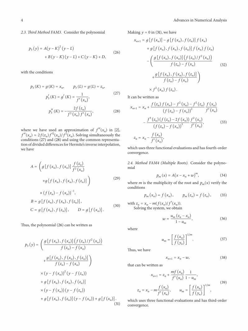
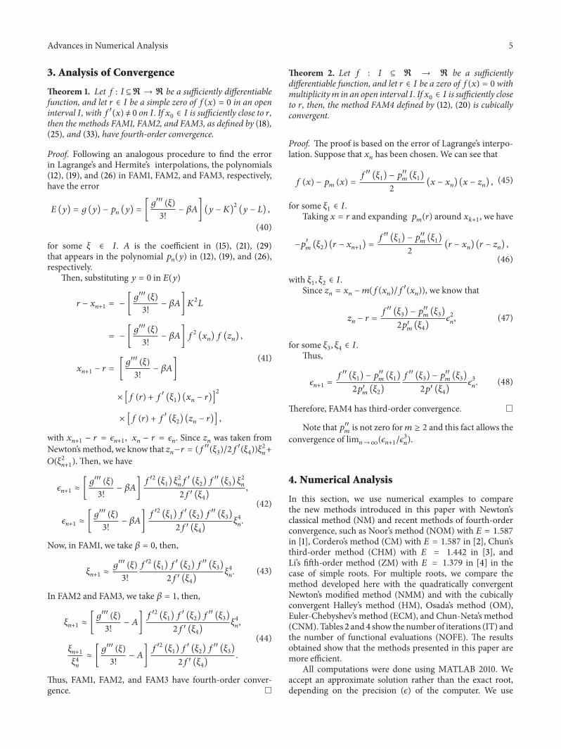
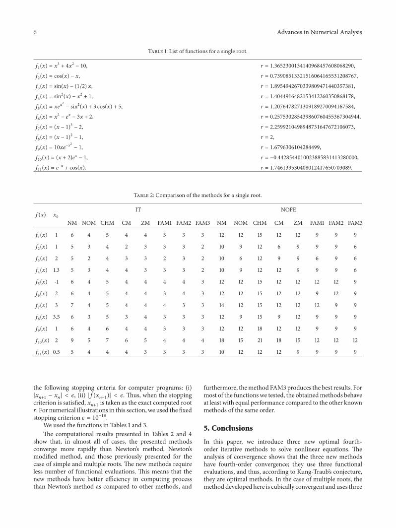
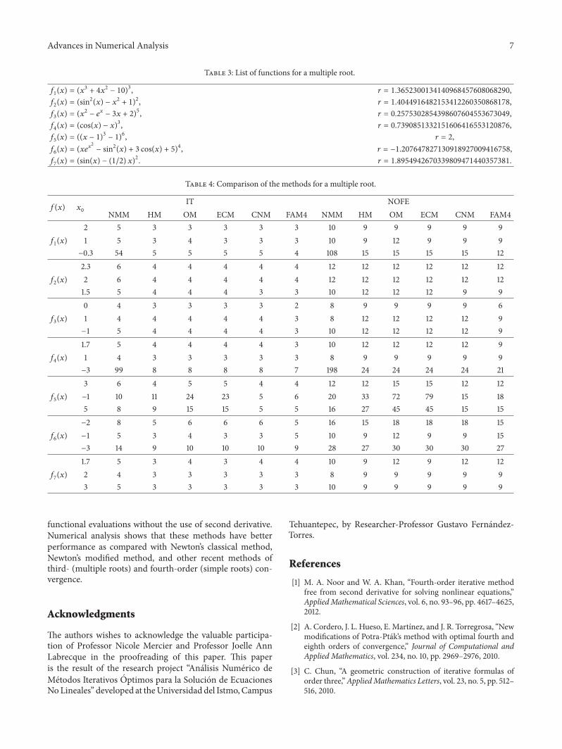