RESEARCH ARTICLES

CURRENT SCIENCE, VOL. 101, NO. 8, 25 OCTOBER 2011 1036

*For correspondence. (e-mail: vssingh77@hotmail.com)

Effectiveness of 3D geoelectrical resistivity imaging using parallel 2D profiles A. P. Aizebeokhai1, A. I. Olayinka2, V. S. Singh3,* and C. C. Uhuegbu1 1Department of Physics, Covenant University, Ota, Ogun State, Nigeria 2Department of Geology, University of Ibadan, Ibadan, Nigeria 3National Geophysical Research Institute (CSIR), Uppal Road, Hyderabad 500 007, India

Acquisition geometry for 3D geoelectrical resistivity imaging in which apparent resistivity data of a set of parallel 2D profiles are collated to 3D dataset was evaluated. A set of parallel 2D apparent resistivity data was generated over two model structures. The models, horst and trough, simulate the geological environment of a weathered profile and refuse dump site in a crystalline basement complex respectively. The apparent resistivity data were generated for Wenner–alpha, Wenner–beta, Wenner–Schlumberger, dipole–dipole, pole–dipole and pole–pole arrays with minimum electrode separation, a (a = 2, 4, 5 and 10 m) and inter-line spacing, L (L = a, 2a, 2.5a, 4a, 5a and 10a). The 2D apparent resistivity data for each of the arrays were collated to 3D dataset and inverted using a full 3D inversion code. The 3D imaging capability and resolution of the arrays for the set of parallel 2D profiles are presented. Grid orientation effects are observed in the inversion images produced. Inter-line spacing of not greater than four times the minimum electrode separation gives reasonable inverse models. The resolution of the inverse models can be greatly improved if the 3D dataset is built by collating sets of orthogonal 2D profiles. Keywords: Acquisition geometry, three-dimensional imaging, geoelectrical resistivity, parallel 2D profiles. THE use of 2D/3D geoelectrical resistivity imaging to address a wide variety of hydrological, environmental and geotechnical issues is increasingly popular. The sub-surface geology in environmental and engineering studies is often subtly heterogeneous and multi-scale, such that both lateral and vertical variations of the subsurface properties can be rapid and erratic. The use of vertical electrical sounding is grossly inadequate to map such complex and multi-scale geology. Two-dimensional (2D) geoelectrical resistivity imaging, in which the subsurface is assumed to vary vertically down and laterally along the profile but is constant in the perpendicular direction, has been used to study areas with moderately complex geo-logy1–5. But subsurface features are inherently 3D and the

2D assumption is commonly violated. This violation often leads to out-of-plane resistivity anomaly in the 2D inverse models, which could be misleading in the inter-pretation of subsurface features6,7. Thus, a 3D geoelectri-cal resistivity imaging which allows resistivity variation in all possible directions should give more accurate and reliable inverse resistivity models of the subsurface, especially in highly heterogeneous cases. The composition of a 3D dataset that would yield signi-ficant 3D subsurface information is less understood. Ideally, a complete 3D dataset of apparent resistivity should be made in all possible directions. In the recent past the techniques for conducting 3D electrical resisti-vity surveys have been presented8. The use of pole–pole8–10 and pole–dipole11,12 arrays has been reported. Square and rectangular grids of electrodes with constant spacing in both the x- and y-directions, in which each electrode is in turn used as the current electrode and the potential meas-ured at all other electrode positions, were commonly used. But these methods which allow the measurement of complete 3D datasets are usually impractical due to the length of cables, the number of electrodes and the site geometry involved in most practical surveys. Also, the measurement of complete 3D datasets using the square or rectangular grids of electrodes is time-consuming and cumbersome in surveys involving large grids. This is because the number of possible electrode permutations for the measurements will be large. To reduce the number of data measurements as well as the time and effort required for 3D geoelectrical resisti-vity field surveys, a cross-diagonal surveying technique in which apparent resistivity measurements are made only at the electrodes along the x-axis, y-axis and 45° diagonal lines was proposed8. The cross-diagonal surveying method also involves a large number of independent measure-ments for medium to large grids of electrodes. Hence, the measurement of 3D dataset using cross-diagonal tech-nique is time-consuming, especially if a single channel or a manual data acquisition system is employed. The inver-sion of these large volumes of data is often problematic because the computer memory may not be sufficient for the data inversion. In contrast to the cross-diagonal sur-veying method, a set of orthogonal 2D lines5–7,13, that allows flexible survey design, choice of array and easy

RESEARCH ARTICLES

CURRENT SCIENCE, VOL. 101, NO. 8, 25 OCTOBER 2011 1037

adaptability to data acquisition systems has been used for 3D geoelectrical resistivity imaging. In this article, Wenner–alpha (WA), Wenner–beta (WB), Wenner–Schlumberger (WSC), dipole–dipole (DDP), pole–dipole (PDP) and pole–pole (PP) arrays were used to generate apparent resistivity data in a set of parallel 2D profiles over two synthetic models, horst and trough. The two models simulate the geological conditions of a weathered profile and refuse dump site in a crystalline basement complex respectively, which are often associ-ated with geophysical applications for hydrogeological, environmental and engineering studies. The calculated apparent resistivity data of the parallel set of 2D profiles over the models were collated to 3D datasets for each array studied and processed using a full 3D inversion code8,14. The imaging capabilities of the parallel set of 2D profiles for 3D surveys were evaluated. The responses of these model structures to 3D inversion for the different arrays were assessed using the 3D inverse models. Dif-ferences in the spatial resolution of the arrays, tendency to produce near-surface artefacts in the 3D inverse mod-els and the deviation from true resistivity models as well as the optimum spacing between the parallel set of 2D lines (inter-line spacing) relative to the minimum elec-trode separation required to form 3D datasets that would yield significant information in 3D inverse models have been evaluated.

Methods of study

Description of the synthetic models

In this study, two model geometries, horst and trough models that represent the geological conditions of a typical weathered profile and refuse dump site in a crystalline basement complex in tropical areas were designed. These geological conditions are often associated with geophysi-cal applications to hydrogeological, environmental and engineering studies. The horst structure with a finite lat-eral extent (Figure 1 a) varies laterally in thickness such that it thickens towards the centre where the least weath-ering is thought to occur and is found to become thinner outward with increasing weathering activities. The horst structure consists of a three-layer model comprising the topsoil, saprolite (the weathered zone) and the fresh basement. The top layer, corresponding to the topsoil, was assigned a uniform thickness of 2.5 m and its resis-tivity varies laterally between 500, 700 and 400 Ωm in the west-east direction. Varying lateral degrees of weath-ering or fracturing that increases outward were assigned to the weathered zone (middle layer) with thickness rang-ing from a minimum of 5.75 m (depth 8.25 m) at the cen-tre of the model structure where the least weathering occurs to a maximum of 13.50 m (depth 16.0 m) at the edges of the model considered to be the most weathered.

The weathered zone in the crystalline basement complex is a product of chemical weathering which is usually a low resistive saprolite overlying a more resistive base-ment rocks15,16 and the zone is commonly aquiferous; thus low values of resistivity ranging from a minimum of 150 Ωm to a maximum of 100 Ωm were assigned. Underlying the weathered zone is a fresh basement of infinite thickness with a constant model resistivity of 3000 Ωm. Horizontal depth slices of the actual model resistivities are given in Figure 2 a. Similarly, the trough structure of finite lateral extent (Figure 1 b) consists of a three-layer model in which the thickness of the top and the middle layers varies to a maximum of 4.2 m and 11.8 m respectively, and the un-derlying layer is a basement rock of infinite thickness. The trough structure varies laterally in thickness and cuts across the first and second layers. Model resistivities of 300 and 600 Ωm were assigned to the first and second layers in their natural states. The trough structure and its surroundings are thought to be impacted by the deposited waste in the simulated dump site and hence would consist of laterally varying low model resistivity. Model resistiv-ity varying laterally between 50 and 250 Ωm, different from the assigned values of 300 and 600 Ωm in its natural state, was therefore assigned to the trough structure. Part of the second layer underlying the trough structure is also thought to be impacted by leachates from the deposited waste, so that its model resistivity varies to a minimum of 400 Ωm from the assigned value of 600 Ωm in its natural state. A constant model resistivity of 2500 Ωm was assigned to the underlying basement of infinite thickness since the leachates from the deposited waste were consid-ered not to have reached the basement. Horizontal depth slices of the actual model resistivities are presented in Figure 2 b.

Apparent resistivity pseudosections

The model structures were approximated into a series of parallel 2D model structures separated with a constant in-terval. Apparent resistivity data were computed over the set of 2D profiles using the finite difference method8,17 for the following arrays: WA, WB, WSC, DDP, PDP and PP. Electrode layouts with minimum separation, a (a = 2, 4, 5 and 10 m) and inter-line spacing, L (L = a, 2a, 2.5a, 4a, 5a and 10a) were used in the computation of the apparent resistivity data. The 2D models were subdivided into a number of homogeneous and isotropic blocks using a rectangular mesh. The resistivity of each of the models was allowed to vary arbitrarily along the profile and with depth, but with an infinite perpendicular extension. The finite dif-ference method basically determines the potential at the nodes of the rectangular mesh. The apparent resistivity values were normalized with the values of a homogeneous

RESEARCH ARTICLES

CURRENT SCIENCE, VOL. 101, NO. 8, 25 OCTOBER 2011 1038

Figure 1. Synthetic models: a, Horst model simulating a typical weathered or fractured profile developed above crystal-line basement complex. b, Trough model simulating the geology of a waste dump site.

Figure 2. Horizontal depth slices of actual model resistivities for (a) the horst structure and (b) the trough structure. earth model so as to reduce the errors in the computed po-tential values. The forward modelling grid used consists of four nodes per unit electrode. Also, 5% Gaussian noise18 was added to the computed apparent resistivity data for each 2D profile so as to simulate field conditions.

Data collation and inversion

The apparent resistivity data computed for the set of par-allel 2D profiles were collated to 3D dataset. The colla-tions arranged the apparent resistivity data and the

RESEARCH ARTICLES

CURRENT SCIENCE, VOL. 101, NO. 8, 25 OCTOBER 2011 1039

electrode layouts in square grids according to the coordi-nates and direction of each 2D profile used, and electrode positions in the profiles. Thus, the size and pattern of the electrode grid depend on the number of electrode in each 2D profile and the number of profiles collated. The col-lated 3D datasets were inverted using a 3D resistivity inversion code8,14 which automatically determines a 3D inverse model of resistivity distribution using apparent resistivity data obtained from a 3D resistivity survey9,19. Ideally, the electrodes used for such surveys are arranged in squares or rectangular grids. Smoothness con-strained inversion method was employed in inverting the datasets. The mesh sizes for the 3D inversion are based on the grid sizes of the collated datasets. However, the mesh sizes are much less than those for the corresponding 3D datasets that would be collated from orthogonal 2D profiles or those of the conventional square or rectangular 3D surveys. The inversions were carried out to study the resolution power of the 3D survey using parallel 2D lines and the effects of different line spacing. The inversion routine used is based on the implementation of the smoothness constrained least-squares method20,21.

Results

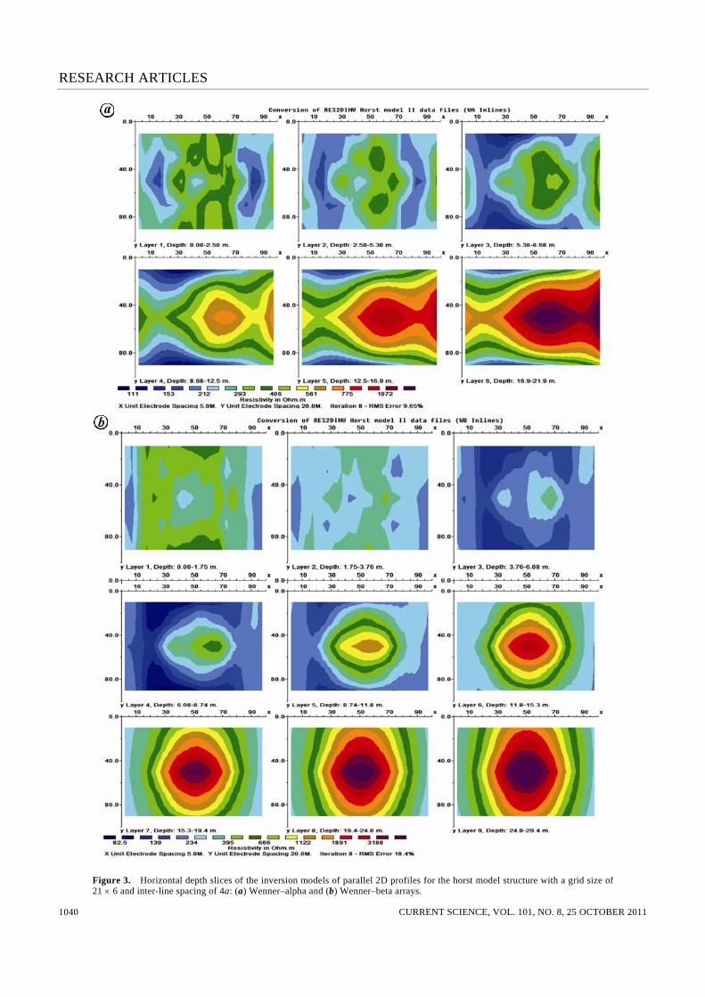
The 3D inversion model resistivity obtained for electrode grid sizes of 21 × 6 with inter-line spacing of 4 a, a being the minimum electrode separation, is presented as a rep-resentative of the inversion models. Horizontal depth slices of the 3D inverse model resistivity of the horst structure for the selected arrays are given in Figures 3–5. Actual model resistivities of the horst structure are given in Figure 2 a. Similarly, the inversion models obtained for electrode grid sizes of 26 × 6 with inter-line spacing of 5a, are presented as representatives of the inverse models for the trough structures. Horizontal depth slices of the 3D inverse model resistivity for the selected arrays are given in Figures 6–8. Actual model sensitivity values of the trough structure are given in Figure 2 b. The resistivity models of the inverse models presented in Figures 3–5 are given in Figures 9–11. The sensitivity models for the various electrode arrays are given in Figures 12–14.

Discussion

The use of parallel 2D profiles in 3D geoelectrical resis-tivity imaging provides a fast and cost-effective tool for site characterization and can be used in subsurface studies for environmental and engineering applications. A com-parison of the images obtained from the 3D inversion of the parallel 2D profiles (horizontal depth slices present in Figures 3–5, and Figures 6–8) to the actual model resis-tivities (Figures 1 and 2 a) shows that 3D imaging using

parallel 2D profiles is relatively efficient. The resolution of the 3D inversion images increases with decreasing inter-line spacing between the 2D profiles. Inter-line spacing of the order of four times the minimum electrode separation would yield inversion images with acceptable resolution5,7. The resolution of the 3D inverse models can be greatly improved if an orthogonal set of 2D profiles is used. The inter-line spacing need not be the same in both directions; and the time and resources available for the survey should, to a large extent, determine the inter-line spacing to be used relative to the minimum electrode separation in both directions. If a sparse set of parallel 2D profiles is used for the 3D survey, the time required for the survey would be signifi-cantly reduced; but this is at the expense of the resolution of the 3D inverse models. The set of parallel 2D profiles could result in small-scale near-surface spurious artefacts in the inverse resistivity models due to the projection of the anomalies located in the deeper parts of the models. However, such 3D inverse models could provide useful information in the interpretation of 3D variation of the subsurface resistivity/conductivity as well as 3D subsur-face features. Thus meaningful 3D information on the subsurface features can be extracted from the 3D inverse models. Grid orientation effect was observed in both structures studied. The inverse models were observed to be oriented perpendicular to the direction of the parallel 2D profiles. The grid orientation effect is independent of the subsur-face features to be mapped. This is evident in the inver-sion images of the two models, horst and trough, presented in this study. The observed grid orientation effects could be misleading in the interpretation of sub-surface features. The effect of grid orientation decreases with decreasing profiles inter-line spacing relative to the minimum electrode separation. Thus, the effect of grid orientation could be minimized or completely eliminated if closely spaced 2D profiles are used relative to the minimum electrode spacing. Also, the grid orientation effects could be minimized using orthogonal 2D profiles to build the 3D dataset without necessarily using the same minimum electrode separation and inter-line spac-ing in both the x- and y-directions5,7. The model sensitivities of the dataset for each array were assessed (Figures 9–14). WB and WSC arrays showed higher and more uniform model sensitivities in the sensitivity maps. However, low model sensitivities were observed at the edges of the sensitivity maps. The model sensitivity of the WA array decreased sharply with depth. The model sensitivities of DDP and PDP arrays were moderate, though edge effects were also observed in the sensitivity maps of these arrays. In general, PP array showed the least model sensitivities in the inversion models; unrealistic edge effects were also observed in the sensitivity of the arrays.

RESEARCH ARTICLES

CURRENT SCIENCE, VOL. 101, NO. 8, 25 OCTOBER 2011 1040

Figure 3. Horizontal depth slices of the inversion models of parallel 2D profiles for the horst model structure with a grid size of 21 × 6 and inter-line spacing of 4a: (a) Wenner–alpha and (b) Wenner–beta arrays.

RESEARCH ARTICLES

CURRENT SCIENCE, VOL. 101, NO. 8, 25 OCTOBER 2011 1041

Figure 4. Horizontal depth slices of inversion models of parallel 2D profiles for horst model structure with a grid size of 21 × 6 and inter-line spacing of 4a: (a) Wenner–Schlumberger and (b) dipole–dipole arrays.

RESEARCH ARTICLES

CURRENT SCIENCE, VOL. 101, NO. 8, 25 OCTOBER 2011 1042

Figure 5. Horizontal depth slices of inversion models of parallel 2D profiles for horst model structure with a grid size of 21 × 6 and inter-line spacing of 4a: (a) pole–dipole and (b) pole–pole arrays.

RESEARCH ARTICLES

CURRENT SCIENCE, VOL. 101, NO. 8, 25 OCTOBER 2011 1043

Figure 6. Horizontal depth slices of the inversion models of parallel 2D profiles for the trough model structure with a grid size of 26 × 6 and inter-line spacing of 5a: (a) Wenner–alpha and (b) Wenner–beta arrays.

RESEARCH ARTICLES

CURRENT SCIENCE, VOL. 101, NO. 8, 25 OCTOBER 2011 1044

Figure 7. Horizontal depth slices of the inversion models of parallel 2D profiles for the trough model structure with a grid size of 26 × 6 and inter-line spacing of 5a: (a) Wenner–Schlumberger and (b) dipole–dipole arrays.

RESEARCH ARTICLES

CURRENT SCIENCE, VOL. 101, NO. 8, 25 OCTOBER 2011 1045

Figure 8. Horizontal depth slices of the inversion models of parallel 2D profiles for the trough model structure with a grid size of 26 × 6 and inter-line spacing of 5a: (a) pole–dipole and (b) pole–pole arrays.

RESEARCH ARTICLES

CURRENT SCIENCE, VOL. 101, NO. 8, 25 OCTOBER 2011 1046

Figure 9. Horizontal depth slices of the sensitivity models of parallel 2D profiles for the horst model structure with a grid size of 21 × 6 and inter-line spacing of 4a: (a) Wenner–alpha and (b) Wenner–beta arrays.

RESEARCH ARTICLES

CURRENT SCIENCE, VOL. 101, NO. 8, 25 OCTOBER 2011 1047

Figure 10. Horizontal depth slices of the sensitivity models of parallel 2D profiles for the horst model structure with a grid size of 21 × 6 and inter-line spacing of 4a: (a) Wenner–Schlumberger and (b) dipole–dipole arrays.

RESEARCH ARTICLES

CURRENT SCIENCE, VOL. 101, NO. 8, 25 OCTOBER 2011 1048

Figure 11. Horizontal depth slices of the sensitivity models of parallel 2D profiles for the horst model structure with a grid size of 21 × 6 and inter-line spacing of 4a: (a) pole–dipole and (b) pole–pole arrays.

RESEARCH ARTICLES

CURRENT SCIENCE, VOL. 101, NO. 8, 25 OCTOBER 2011 1049

Figure 12. Horizontal depth slices of the sensitivity models of parallel 2D profiles for the trough model structure with a grid size of 21 × 6 and inter-line spacing of 4a: (a) Wenner–alpha and (b) Wenner–beta arrays.

RESEARCH ARTICLES

CURRENT SCIENCE, VOL. 101, NO. 8, 25 OCTOBER 2011 1050

Figure 13. Horizontal depth slices of the sensitivity models of parallel 2D profiles for the trough model structure with a grid size of 21 × 6 and inter-line spacing of 4a: (a) Wenner–Schlumberger and (b) dipole–dipole arrays.

RESEARCH ARTICLES

CURRENT SCIENCE, VOL. 101, NO. 8, 25 OCTOBER 2011 1051

Figure 14. Horizontal depth slices of the sensitivity models of parallel 2D profiles for the trough model structure with a grid size of 21 × 6 and inter-line spacing of 4a: (a) pole–dipole and (b) pole–pole arrays.

RESEARCH ARTICLES

CURRENT SCIENCE, VOL. 101, NO. 8, 25 OCTOBER 2011 1052

Conclusion

The use of parallel 2D profiles in generating 3D dataset is a fast and cost-effective technique of conducting 3D geoelectrical resistivity surveys. The inter-line spacing should not be greater than four times the minimum elec-trode separation for good quality and high-resolution 3D inversion images. The resolution of the inversion images can be enhanced by using closely spaced 2D profiles or orthogonal 2D profiles. The model sensitivities of the in-verse models indicate that WB, WSC and DDP arrays are more sensitive to the 3D features, while PP array is least sensitive to the 3D features. The inverse models are, however, characterized with grid orientation effects which can be misleading in the interpretation of subsur-face features. The grid orientation effect can be mini-mized by reducing the inter-line spacing relative to the minimum electrode separation or eliminated by collating orthogonal 2D profiles to the 3D dataset.

1. Griffiths, D. H. and Barker, R. D., Two dimensional resistivity imaging and modeling in areas of complex geology. J. Appl. Geo-phys., 1993, 29, 211–226.

2. Dahlin, T. and Loke, M. H., Resolution of 2D Wenner resistivity imaging as assessed by numerical modelling. J. Appl. Geophys., 1998, 38(4), 237–248.

3. Olayinka, A. I. and Yaramanci, U., Choice of the best model in 2-D geoelectrical imaging: case study from a waste dump site. Eur. J. Environ. Eng. Geophys., 1999, 3, 221–244.

4. Amidu, S. A. and Olayinka, A. I., Environmental assessment of sewage disposal systems using 2D electrical resistivity imaging and geochemical analysis: a case study from Ibadan, Southwestern Nigeria. Environ. Eng. Geosci., 2006, 7(3), 261–272.

5. Aizebeokhai, A. P., Olayinka, A. I. and Singh, V. S., Application of 2D and 3D geoelectrical resistivity imaging for engineering site investigation in a crystalline basement terrain, southwestern Nigeria. J. Environ. Earth Sci., 2010, 61, 1481–1492.

6. Bentley, L. R. and Gharibi, M., Two- and three-dimensional elec-trical resistivity imaging at a heterogeneous site. Geophysics, 2004, 69(3), 674–680.

7. Gharibi, M. and Bentley, L. R., Resolution of 3D electrical resis-tivity images from inversion of 2D orthogonal lines. J. Environ. Eng. Geophys., 2005, 10(4), 339–349.

8. Loke, M. H. and Barker, R. D., Practical techniques for 3D resis-tivity surveys and data inversion. Geophys. Prospect., 1996, 44, 499–524.

9. Li, Y. and Oldenburg, D. W., Inversion of 3D DC resistivity data using an approximate inverse mapping. Geophys. J. Int., 1994, 116, 527–537.

10. Park, S., Fluid migration in the vadose zone from 3D inversion of resistivity monitoring data. Geophysics, 1998, 63, 41–51.

11. Chambers, J. E., Ogilvy, R. D., Meldrum, P. I. and Nissen, J., 3D electrical resistivity imaging of buried oil–tar contaminated waste deposits. Eur. J. Environ. Eng. Geophys., 1999, 4, 3–15.

12. Ogilvy, R., Meldrum, P. and Chambers, J., Imaging of industrial waste deposits and buried quarry geometry by 3D tomography. Eur. J. Environ. Eng. Geophys., 1999, 3, 103–113.

13. Aizebeokhai, A. P., Olayinka, A. I. and Singh, V. S., Numerical evaluation of 3D geoelectrical resistivity imaging for environ-mental and engineering investigations using orthogonal 2D pro-files. SEG Expanded Abstracts, 2009, 28, 1440–1444.

14. Loke, M. H. and Dahlin, T., A comparison of the Gauss–Newton and quasi-Newton methods in resistivity imaging inversion. J. Appl. Geophys., 2002, 49(3), 149–162.

15. Carruthers, R. M. and Smith, I. F., The use of ground electrical survey methods for sitting water supply boreholes in shallow crys-talline basement terrain. In Hydrogeology of Crystalline Basement Aquifers in Africa (eds Wright, E. P. and Burgess, W. G.), Geo-logical Society Special Publication, 1992, vol. 66, pp. 203–220.

16. Hazell, J. R. T., Cratchley, C. R. and Jones, C. R. C., The hydrol-ogy of crystalline aquifers in northern Nigeria and geophysical techniques used in their exploration. In Hydrogeology of Crystal-line Basement Aquifers in Africa (eds Wright, E. P. and Burgess, W. G.), Geological Society Special Publication, 1992, vol. 66, pp. 155–182.

17. Dey, A. and Morrison, H. F., Resistivity modelling for arbitrary shaped two-dimensional structures. Geophys. Pros., 1979, 27, 1020–1036.

18. Press, W. H., Teukolsky, S. A., Vetterling, W. T. and Flannery, B. P., Numerical Recipes in Fortran 77: The Art of Scientific Com-puting, Cambridge University Press, Cambridge, 1996, 2nd edn.

19. White, R. M. S., Collins, S., Denne, R., Hee, R. and Brown, P., A new survey design for 3D IP modelling at Copper hill. Explor. Geophys., 2001, 32, 152–155.

20. De Groot-Hedlin, C. and Constable, S. C., Occam’s inversion to generate smooth two dimensional models from magnetotelluric data. Geophysics, 1990, 55, 1613–1624.

21. Sasaki, Y., Resolution of resistivity tomography inferred from numerical simulation. Geophys. Prospect., 1992, 40, 453–464.

ACKNOWLEDGEMENTS. The Third World Academy of Science (TWAS), Italy, and the Council of Scientific and Industrial Research (CSIR), India are gratefully acknowledged by the first author for pro-viding a fellowship for this study at the National Geophysical Research Institute, Hyderabad, India. Received 24 January 2011; revised accepted 5 September 2011