SWANSEA UNIVERSITY

Environmental Dynamics and Climate Change

M.Sc. PROJECT

An Evaluation of the Climatic Signal within the

Earlywood Vessel Area of Quercus petraea (Matt.)

Liebl.

STUDENT NAME: Darren Davies

STUDENT NUMBER: 552192

SUPERVISOR: Dr Neil Loader

YEAR OF SUBMISSION: 2013

This work is part-funded by the European Social Fund (ESF) through the

European Union’s Convergence program administered by the Welsh

Government

I

Abstract

This paper investigated the climatic signals contained within earlywood vessels of 10

sessile oak trees (Quercus petraea (Matt.) Liebl.) from the UK, a first in the literature,

and their suitability for producing climate reconstructions. For the period of 1860 to

2012, 4 earlywood vessel area chronologies were constructed, along with a ring-width

record. The vessel chronologies were constructed through different combinations of the

largest annual earlywood vessels, allowing examination of how the climatic signals

were expressed. Identification of climatic influences was found by comparison with

monthly meteorological records. In contrast to the ring-width chronology, each vessel

chronology was statistically weaker in terms of common signal, and sensitivity.

However, earlywood vessels were less dependent on previous year growth. Earlywood

vessels were found to contain a different climatic signal to ring-widths, suggesting merit

in their use at this location. March relative humidity demonstrated the greatest influence

on earlywood vessel area, however, this signal was different between series, indicating

that different groupings of vessels may affect the expressed signal. Examination of the

suitability of the earlywood vessel chronologies to produce a March relative humidity

reconstruction demonstrated that chronologies composed of all earlywood vessels and

those with less than 5 were unsuitable. However, a chronology consisting of the average

of the 10 largest earlywood vessels was found to produce a stable reconstruction,

resulting in a March relative humidity reconstruction for the study period. Results

indicate promise in the use of earlywood vessels as a climatic proxy within the UK. As

a result of this study further research directions are suggested.

Key Words: Earlywood Vessels; Climate Proxy; Relative Humidity; United

Kingdom; Quercus petraea (Matt.) Liebl.

II

Declaration and Statements

This is being submitted in partial fulfilment of the requirements for the degree.

Sign:

Date:

This work has not previously been accepted in substance for any other degree and is not

being concurrently submitted in candidate for any degree.

Sign:

Date:

This dissertation is the result of my own independent work investigation, except where

otherwise stated. Other sources are acknowledged by footnotes giving explicit

references. A Bibliography is appended.

Signed:

Date:

I hereby give my consent for my dissertation, if relevant and accepted to be available for

photocopy, inter-library loan and for the title and summary to be made available to

outside organisations.

Signed:

Date:

Word Count: 6,681

III

Acknowledgements

The author would like to thank Dr Neil Loader for his input and advice throughout the

project, as well as staff at the National Botanic Gardens of Wales, especially Dr Angela

Singleton. In addition, the help afforded by Millie Watts, Siôn Carpenter and Ash

Woodward in collecting samples is much appreciated. Guidance provided by Prof.

Danny McCarroll aided with analysis. Thanks are also extended to Dr Neil Robertson

for his help. The author acknowledges the E-OBS dataset from the EU-FP6 project

ENSEMBLES (http://ensembles-eu.metoffice.com) and the data providers in the

ECA&D project (http://www.ecad.eu). The author is also appreciative of the funding

provided by the European Social Fund (ESF) through the European Union’s

Convergence program administered by the Welsh Government.

IV

Contents Page

Abstract I

Declaration and Statement II

Statement of Word Count II

Acknowledgements III

Table of Contents IV

List of Abbreviations V

List of Figures VI

List of Tables VIII

Section 1 – Introduction 1

Section 2 – Methodology 8

2.1 – Site location 8

2.2 – Sample Selection, Preparation and Measurement 8

2.3 – Chronology Construction and Climate-Growth Analysis 10

2.4 – Examination of Suitability for Climate Reconstruction 13

Section 3 – Results 14

3.1 – Vessel Characteristics 14

3.2 – Chronology Analysis 14

3.3 – Climate-Growth Relationships 17

3.4 – Climate Reconstruction 20

Section 4 – Discussion 21

Section 5 – Conclusion 30

References 32

Supplementary Information 39

Administrative Appendices 49

Appendix A – SOTEAS Risk Assessment 49

Appendix B – Meeting Log 53

V

List of Abbreviations

Coefficient of Efficiency CE

Estimated Sample Depth ESD

Expressed Population Signal EPS

First Order Autocorrelation AutoR

Mean Between Tree Correlation Rbt

Mean Sensitivity MS

National Botanic Gardens of Wales NBGW

Reduction of Error RE

Ring-Width RW

VI

List of Figures

Page Number

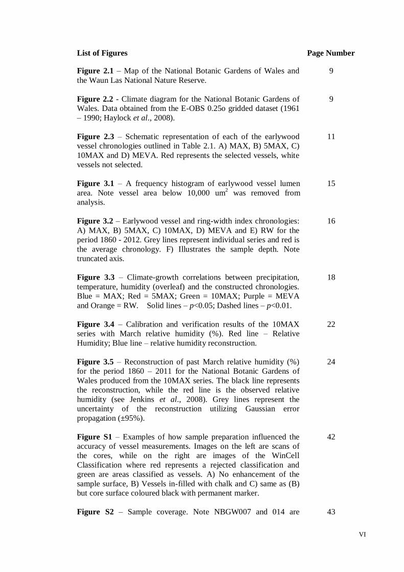
Figure 2.1 – Map of the National Botanic Gardens of Wales and

the Waun Las National Nature Reserve.

9

Figure 2.2 - Climate diagram for the National Botanic Gardens of

Wales. Data obtained from the E-OBS 0.25o gridded dataset (1961

– 1990; Haylock et al., 2008).

9

Figure 2.3 – Schematic representation of each of the earlywood

vessel chronologies outlined in Table 2.1. A) MAX, B) 5MAX, C)

10MAX and D) MEVA. Red represents the selected vessels, white

vessels not selected.

11

Figure 3.1 – A frequency histogram of earlywood vessel lumen

area. Note vessel area below 10,000 um2 was removed from

analysis.

15

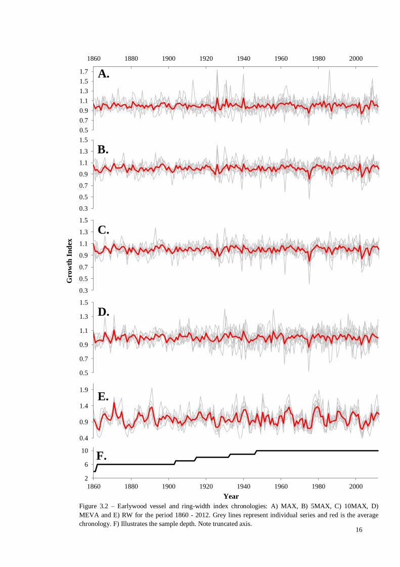
Figure 3.2 – Earlywood vessel and ring-width index chronologies:

A) MAX, B) 5MAX, C) 10MAX, D) MEVA and E) RW for the

period 1860 - 2012. Grey lines represent individual series and red is

the average chronology. F) Illustrates the sample depth. Note

truncated axis.

16

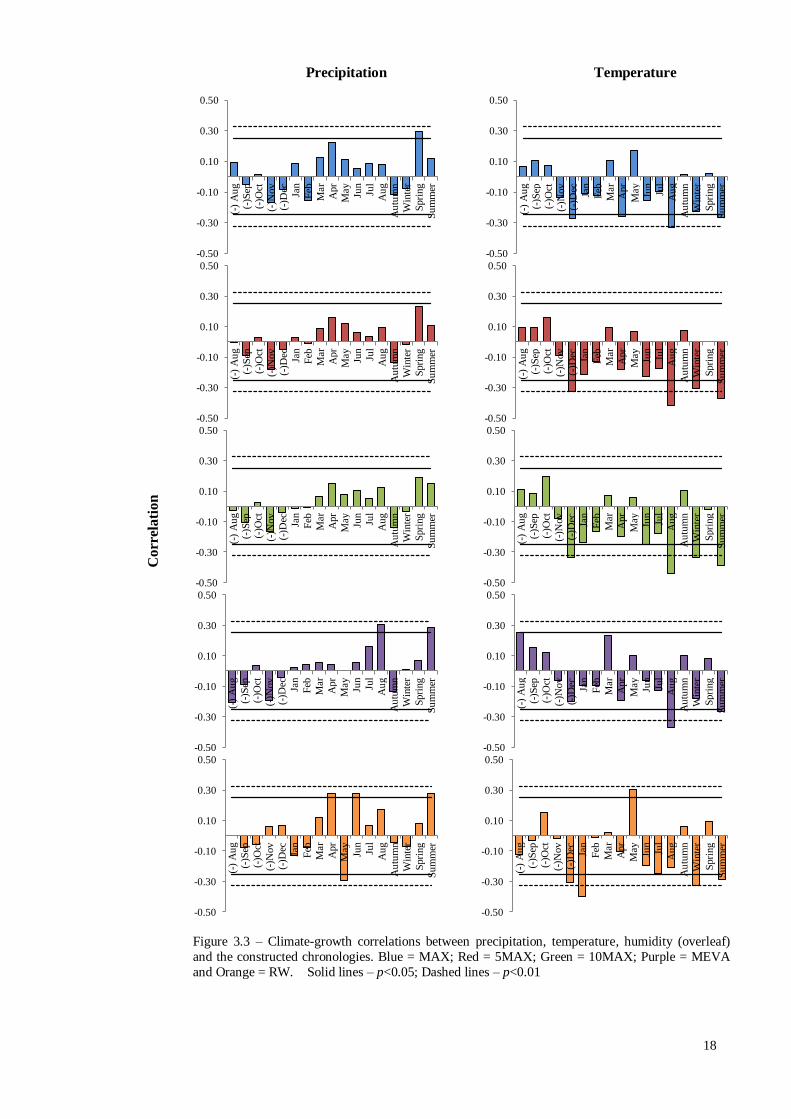
Figure 3.3 – Climate-growth correlations between precipitation,

temperature, humidity (overleaf) and the constructed chronologies.

Blue = MAX; Red = 5MAX; Green = 10MAX; Purple = MEVA

and Orange = RW. Solid lines – p<0.05; Dashed lines – p<0.01.

18

Figure 3.4 – Calibration and verification results of the 10MAX

series with March relative humidity (%). Red line – Relative

Humidity; Blue line – relative humidity reconstruction.

22

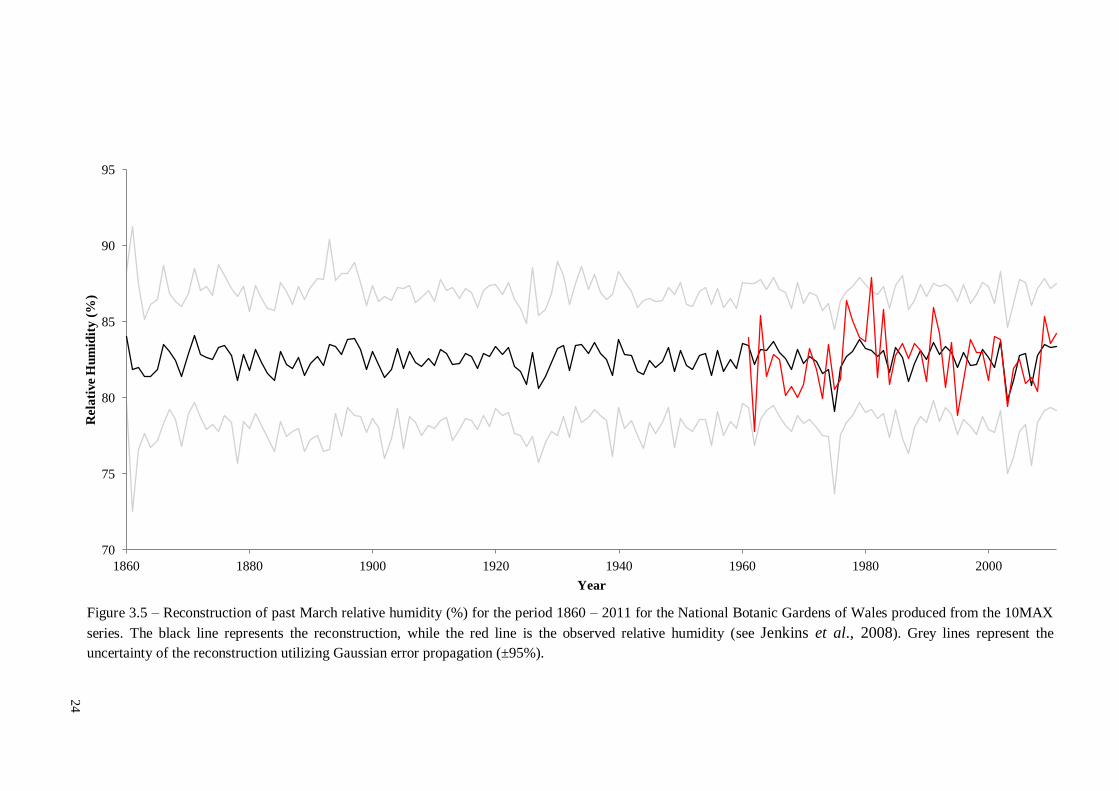
Figure 3.5 – Reconstruction of past March relative humidity (%)

for the period 1860 – 2011 for the National Botanic Gardens of

Wales produced from the 10MAX series. The black line represents

the reconstruction, while the red line is the observed relative

humidity (see Jenkins et al., 2008). Grey lines represent the

uncertainty of the reconstruction utilizing Gaussian error

propagation (±95%).

24

Figure S1 – Examples of how sample preparation influenced the

accuracy of vessel measurements. Images on the left are scans of

the cores, while on the right are images of the WinCell

Classification where red represents a rejected classification and

green are areas classified as vessels. A) No enhancement of the

sample surface, B) Vessels in-filled with chalk and C) same as (B)

but core surface coloured black with permanent marker.

42

Figure S2 – Sample coverage. Note NBGW007 and 014 are 43

VII

missing years.

Figure S3 - Spatial field analysis of August temperatures for the

period of 1951-2012 against the A) MAX, B) 5MAX, C) 10MAX

and D) MEVA chronologies. Produced through KNMI Climate

Explorer (http://climexp.knmi.nl/).

44

VIII

List of Tables

Page Number

Table 2.1 – Description of the constructed earlywood vessel

chronologies.

11

Table 3.1. - Expressed population signal (EPS), Estimated sample

depth for an EPS of 0.85 (ESD), mean correlation between

standardized chronologies (Rbt), mean sensitivity (MS) and first

order autocorrelation coefficient (AutoR) for the common period

(1947 – 2012) for each Q. Petraea (Matt.) L. earlywood vessel

chronology.

15

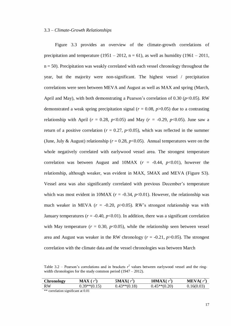
Table 3.2 – Pearson’s correlations and in brackets r2 values

between earlywood vessel and the ring-width chronologies for the

study common period (1947 – 2012).

17

Table 3.3 – An overview of the verification statistics used to

analyse the relationship between relative humidity and each

constructed chronology (1961 – 2011). Forward model: Calibration

period 1986 – 2011, verification period 1961 – 1985. Reverse

model: Calibration period 1961 – 1985, verification period 1986 –

2011.

20

Table S1 – Tree sample meta-data.

45

Table S2 -Filters used to identify and control abnormal

classifications.

46

1

1. Introduction

Anthropogenic activities over the last two centuries have amplified average global

temperatures by an estimated 0.7 oC (Solomon et al., 2007). One of the consequences

that have been hypothesised is a rise in extreme weather events, such as; heavy

precipitation and drought (e.g. Salinger & Griffiths, 2001; Allan & Soden, 2008;

Coumou & Rahmstorf, 2012; Westra et al., 2013). Therefore, global warming will

negatively impact the human and natural environment in the future (e.g. increased

spread of disease and reduced biodiversity; see McMichael et al., 2006 and Bellard et

al., 2012). The climate models from which such conclusions have been drawn are

calibrated and validated through the use of climate observations (Sundberg et al., 2012).

The obvious source of this data is from instrumental stations; however, these records are

temporally and spatially restricted (Ruddiman, 2008. pp. 314). To overcome these

limitations climate proxies are utilized.

Found in a number of archives including; ice cores (e.g. Petit et al., 1999), lake

sediments (e.g. Fritz et al., 1991) and peat cores (e.g. Barber et al., 1994), proxies

contain an indirect record of past climate conditions. However, these proxies do not

have the advantages afforded by tree-rings (McCarroll & Loader, 2004). For example,

as annual rings can be precisely dated, long accurate chronologies can be constructed

(e.g. Friedrich et al., 2007) and through replication, measurements of confidence can be

produced (McCarroll & Loader, 2004; McCarroll et al., 2013). As a consequence, tree

based proxies have been the foundation of a number of significant climate

reconstructions (e.g. Mann et al., 1999; Esper et al., 2002; Moberg et al., 2005).

Tree-ring width measurements have traditionally been used as a proxy (Campelo

et al., 2010), while more recently earlywood and latewood width (e.g. Kalela-Brundin,

1999), stable isotope measurements (e.g. Burk & Stuiver, 1981) and latewood density

2

(e.g. Briffa et al., 1988) have also been utilized. However, one of the challenges of

producing tree-based proxy reconstructions, and with climate proxies in general, is the

production of intra-annual reconstructions (Campelo et al., 2010). Such investigations

have utilized frost- and double-ring incidences (e.g. Brunstein, 1996; Campelo et al.,

2007), however; these approaches are limited. Thus, a frontier in contemporary

dendroclimatology is the identification of high resolution proxies, with anatomical tree-

ring features being cited as a promising research avenue (García-González & Fonti,

2006).

Wood cell features (i.e. diameter and lumen area) have long been recognised to be

modified between locations and along climatic gradients (Fonti & García-González,

2004), and through producing time-series of these characteristics it is hypothesised that

environmental information can be obtained (Schweingruber, 2001; Fonti et al., 2009).

The environmental signal within wood cell features is thought to be related to water

quantities within the tree. As water levels rise, turgor pressure increases, which will

influence the cell size (Ray et al., 1972; Boyer, 1985; Eilmann et al., 2006). However,

constraints (i.e. cost and time) have impeded the production of accurate measurements

of such features, and thus producing chronologies (Eckstein, 2004). Therefore, the

science was slow to develop until the invent of semi- and fully-automatic image

analysis systems (Eckstein, 2004). Consequently, since the latter half of the twentieth

century, there have been a number of investigations relating cell characteristics to

environmental signals, especially the water-conducting elements of conifers (e.g.

Panyushkina et al., 2003; DeSoto et al., 2011). However, similar research with

angiosperm species is lacking (Fonti & García-González, 2004).

Historically, the study of hardwood vessels was considered a technique to

differentiate between wood species, and it was sometime before it was documented that

3

over extended periods, vessel characteristics evolved with environmental influences

(Carlquist, 1988; Eckstein, 2004). However, early studies established that vessel

features were modified following extreme climatic years (i.e. Knigge & Schulz, 1961)

and that such qualities were suitable for the production of annual time-series (i.e.

Eckstein et al., 1977).

Since these early investigations, a variety of vessel features have been examined

within ring- and semi-ring porous species for an environmental signal. Pumijumnong &

Park (1999) for instance, investigated average vessel area, vessel diameter, and vessel

density in Tectona grandis L., while Tardif & Conciatori (2006) looked at the total

vessel area, largest earlywood vessel area and number of vessels in Quercus alba L. and

Quercus rubra L. The majority of research has however, focused on annual mean vessel

area. St. George et al., (2002) for example, found that reduced annual average vessel

area, within Quercus macrocarpa, to be associated with incidents of flooding. While

Schume et al., (2004) investigated the relationship between ground water and mean

vessel area, and found a reduction in vessel size with a loss of ground water contact. In

recent years however, research has specifically examined the environmental signal

contained within vessels of the earlywood, in the hope that information can be gained

on past spring and early summer events.

Traditionally, earlywood features have been avoided due to difficulties in

identifying an environmental relationship (Fonti & García-González, 2004). However,

earlywood vessels have demonstrated such a signal. For example, evidence supports a

distinct flooding signal within the average earlywood vessel area of different oak

species, representing spring and early summer flooding events (e.g. Astrade & Bégin,

1997; St. Georege & Nielsen, 2000, 2003). The majority of focus, however, has been on

climatic signals. García-González & Eckstein (2003) look explicitly at earlywood

4

vessels for a climatic signal and were able to produce a time-series composed of annual

average earlywood vessel area and found a strong positive spring precipitation signal,

which was mirrored by Eilmann et al., (2006). Contrasting these conclusions, a number

of investigations have found that earlywood vessel area has instead increased with

drought conditions (e.g. Knigge & Schulz, 1961; Pumijumnong & Park, 1999;

Corcuera et al., 2004; García-González & Fonti, 2007; Fonti & García-González, 2008).

On the other hand, a temperature signal has also been documented (e.g. Fonti & García-

Gonzalez, 2004). Both Matisons et al., (2012) and Matisons & Brumelis (2012) found

that winter and spring temperatures in Latvian Q. Robur L. controlled earlywood vessel

area. However, the signal was found to have altered in the recent century to one

dominated by summer precipitation, which was attributed to local climate change.

Eilmann et al., (2006) provides a number of explanations that could account for these

differences, including; different species response to water availability, different site

conditions, the internal control of earlywood production (e.g. Sass & Eckstein, 1995)

and differences in previous year climatic conditions.

Although there are currently difficulties in determining a common vessel response

to climatic conditions between locations and species, research has continued, and it

appears that potentially many of the early studies that took an overall vessel area

average have suffered from a mixing of climatic signals. Vessels are produced through

the growing season, thus are influenced by differing environmental conditions (García-

González & Fonti, 2006), in addition there is hypothesised to be a fixed period in which

vessels can be affected by environmental stimuli, namely, the time between cell

differentiation and the production of the secondary cell wall (Fonti & García-González,

2004). García-González & Fonti (2006) demonstrated that vessels produced at different

times contained contrasting climatic signals. For instance, the authors found that the

5

largest vessels were correlated with temperatures in March, while the smallest were

with June, and by computing an average of all earlywood vessels the correlations were

weakened. However, examining how climate signal strength responded to different

combinations of earlywood vessel areas, García-González & Eckstein (2003) found that

by removing a small proportion of the smallest vessels, the signal was weakened, and

there was no evidence of any improvement by retaining just the largest individuals.

Although the research considered to this point supports the use of vessel area

chronologies for climate reconstructions, some have concluded differently. Fonti et al.,

(2009) investigated the change in climate signal over different frequencies with a vessel

chronology of 446 years, the longest produced to date. By considering the climate signal

at low-, medium- and high-frequencies it was found that the signal was not consistent

throughout the vessel area chronology, where at high frequencies there was a negative

spring response, in contrast to an indirect positive response in the lower frequencies.

Such a response is problematic due to the contrasting signs of the relationship (Fonti et

al, 2009). In addition, an assumption of detrending is that there is a stable climate

response throughout the series, across different frequencies (Esper et al., 2005, 2009;

Fonti et al., 2009). However, when considering this conclusion it is also important to

acknowledge that at this site the authors also reported a similar result with a tree-ring

width chronology. Tree-ring width chronologies have been successfully utilized in

climatic reconstructions from other locations, thus it should be considered that this

result could be location based. For average earlywood vessel area to be considered a

‘useful’ proxy it has been said that the climatic signal contained should be different to

that found in easier to measure features, such as traditional ring-widths (Fonti & García-

González, 2004), a common finding in the literature (e.g. Pumijumnong & Park, 1999;

Fonti & García-González, 2004; Matisons & Brumelis, 2012). In contrast, Tardif &

6

Conciatori (2006) reported that for Q. alba L. and Quercus rubra L. that the average

earlywood vessel area produced a similar, but weaker relationship to growing season

conditions than a constructed ring-width chronology. Thus, at that study location the

production of a vessel chronology provided no benefit. In addition, the suitability of

vessels to produce chronologies should be questioned, as it is common to find that the

statistical quality of vessel chronologies is poor compared to ring-width chronologies.

For example, Fontí & García-González (2008) who compared ring-, latewood- and

earlywood-width to mean vessel area at three locations, found that the common

variability, signal and mean sensitivity was reduced in the vessel chronologies

compared to each width measurement chronology. This theme is repeated across the

literature (e.g. García-González & Eckstein, 2003; Fonti & García-González, 2004;

Tardiff & Conciatori, 2006; Fonti & García-González, 2008; Campelo et al., 2010).

However, it has been argued that the relationship between the proxy and the climate is

more important than the relationship between individual series (e.g. Fonti & García-

González, 2008). Although, this view could be seen as contradictory, as a reduced

common signal between trees will only result in a weakened and blurred signal that is

expressed when chronologies are combined.

From reviewing the literature it is clear that this particular field is still in its

infancy, and there are still many gaps. One of the main focal points that needs further

consideration is the relationship between vessel development and environmental

stimuli. In addition, there is a need to expand on research locations as current studies are

limited in specific areas, with currently none in the UK. To date, the majority of

published research has produced only short vessel chronologies which increases the

chance of spurious relationships with climatic records (e.g. 25 years; García-González

& Fonti, 2007, 22 years; Alla & Camarero, 2012). Thus, longer chronologies need to be

7

produced. Furthermore, the relationship between vessel chronologies and the climate to

date have only been examined with Pearson’s correlations and there is much to be

gained through using statistics such as the Reduction of Error (RE) and Coefficient of

Efficiency (CE; National Research Council, 2007). Such statistics are commonly used

to validate climate reconstructions, and will provide a better illustration of the suitability

of vessel chronologies for such an investigation. Thus, this project aims to:

1. Evaluate the quality of time-series built from average earlywood vessel area,

2. Evaluate, for the first time, the climatic signal contained within earlywood

vessels in the UK by producing an extended average earlywood vessel area

chronology and comparing it to climatic data,

3. Find how different combinations of earlywood vessel sizes affect the expression

of a climate signal,

4. Evaluate the suitability of vessel chronologies for climatic reconstructions in the

UK.

8

2. Methodology

2.1 – Site Location

Samples were collected from within the boundaries of the National Botanic

Gardens of Wales (NBGW) and the adjacent Waun Las National Nature Reserve

(51o50’ N, 04

o08’ W; 87 m a.s.l.; Figure 2.1). According to the National Vegetation

Classification System (Rodwell, 1991, 1992), the vegetation is dominated by semi-

improved grassland and dense scrub woodland (NBGW, 2013). Being a public

attraction there is evidence of minor management of the larger vegetation within the

NBGW limits, while it is minimal in the nature reserve. Average annual temperature is

9.8oC, while total average precipitation is 1365mm, with the majority falling over the

autumn and winter months (1961 – 1990; Figure 2.2) (Haylock et al., 2008).

2.2 – Sample Selection, Preparation and Measurement

Based on physical appearance (i.e. no fallen limbs, no evidence of rot) 10 sessile

oak trees (Quercus petraea (Matt.) Liebl.) were identified for investigation (Table S1).

To ensure a representative sample of earlywood vessels, dual 5-mm cores were obtained

at breast height (1.3 m) from each individual (García-González & Fonti, 2007). To

minimize the risk of reaction wood, cores were removed perpendicular to the

topographic slope (Fonti et al., 2009; Speer, 2010, p.78). Samples were left to air-dry;

before the transversal surface was progressively prepared with sandpaper (P80, P400

and P600 grades). Prior analysis, vessel lumina were cleared with compressed air, while

the wood matrix was coloured black and vessels in-filled with chalk, improving the

contrast for image analysis (e.g. Alla & Camarero, 2012) (see supplementary method).

Ring-widths were visually measured through use of a binocular microscope

(Nikon SMZ645), a Velmex positioning table and the software TSAP (Rinn, 2003),

9

0

20

40

60

80

100

120

140

160

180

0

5

10

15

20

J F M A M J J A S O N D

Tota

l P

recip

ita

tion

(m

m)

Avera

ge T

em

pera

ture (

oC

)

Month

1365 mm 9.8oC

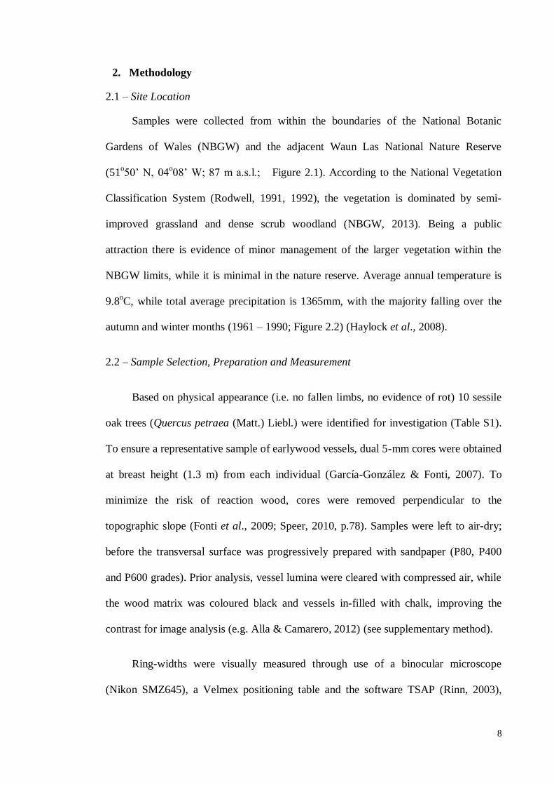
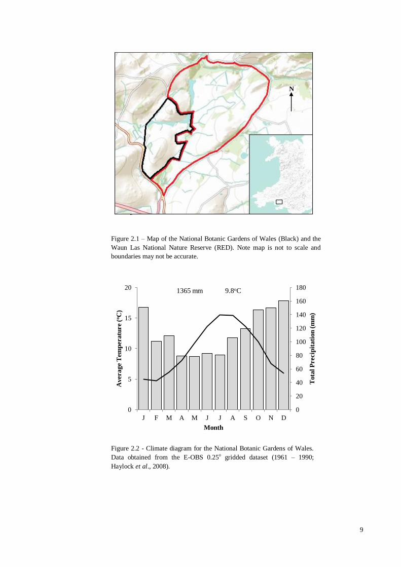
Figure 2.1 – Map of the National Botanic Gardens of Wales (Black) and the

Waun Las National Nature Reserve (RED). Note map is not to scale and

boundaries may not be accurate.

Figure 2.2 - Climate diagram for the National Botanic Gardens of Wales.

Data obtained from the E-OBS 0.25o gridded dataset (1961 – 1990;

Haylock et al., 2008).

N

10

which also produced the master tree-ring chronology (see supplementary information).

Digital images of each core were captured using an EPSON Perfection V750 scanner at

6400 dpi resolution while, vessel analysis was conducted through the WinCELL PRO

(ver. 2013) software (Régents Instruments Inc., Québec, Canada). To ensure the

measurement of earlywood vessels a minimum size filter was applied at 10,000 μm2

(e.g. Fonti & García-González, 2008), while a suite of filters were used to avoid

inaccurate classification of ring features (Table S2).

To verify the accuracy of the chronology dating, independent ring-width

measurements were produced by the WinCELL PRO software and compared to the

original measurements. Due to inaccurate classifications by the image analysis software,

visual inspection of vessel classifications was also conducted and anomalous results

were removed (i.e. combined vessels, remaining debris).

2.3 – Chronology Construction and Climate-Growth Analysis

To examine the effect of selecting different size groups of earlywood vessels on

the climatic signal expressed, four earlywood vessel series were created (Table 2.1;

Figure 2.3), by pooling each dual core together (e.g. García-González & Eckstein,

2003), in addition to an average ring-width chronology. To compute these variables a

purposely designed computer package was created (see supplementary method).

To remove non-climatic, and preserve high frequency signals (Fonti et al., 2007),

a cubic smoothing spline of 32-year stiffness and 50% cut-off was utilized (e.g. Fonti &

García-González, 2004, 2008; Campelo et al., 2010), using the R (R Core Team, 2013)

package DetrendeR (Campelo, 2012). Detrending was applied to all series variables

individually, preventing differences arising due to utilizing contrasting methods

(García-González & Eckstein, 2003). Site chronologies were then computed by

11

Table 2.1 – Description of the constructed earlywood vessel chronologies.

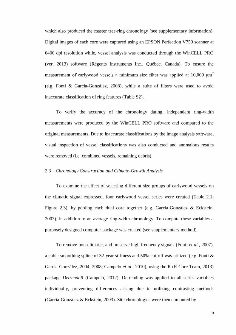
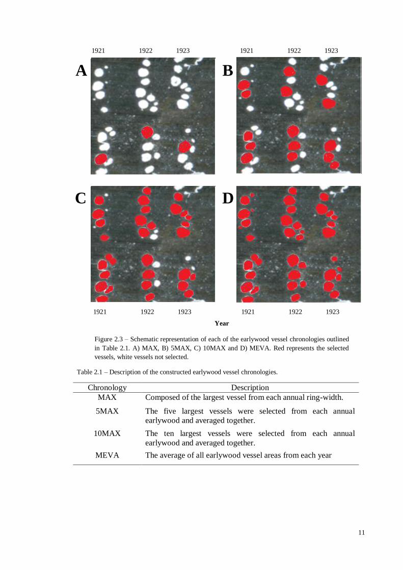
Chronology Description

MAX Composed of the largest vessel from each annual ring-width.

5MAX The five largest vessels were selected from each annual

earlywood and averaged together.

10MAX The ten largest vessels were selected from each annual

earlywood and averaged together.

MEVA The average of all earlywood vessel areas from each year

Year

Figure 2.3 – Schematic representation of each of the earlywood vessel chronologies outlined

in Table 2.1. A) MAX, B) 5MAX, C) 10MAX and D) MEVA. Red represents the selected

vessels, white vessels not selected.

1921 1922 1923 1921 1922 1923

1921 1922 1923 1921 1922 1923

A B

C D

12

averaging all individual series together (e.g. Fonti & García-González, 2008). A

common period between 1947 and 1993 was produced as two trees had single core

coverage from 1993 to 2012 (Figure S2). However, the decision was made to include

these cores to increase coverage to the present, producing a common period between

1947 and 2012 (n = 65).

To review the statistical quality of the chronologies over the studies common

period, a number of statistics were selected which are common in dendroclimatology as

follows (e.g. Campelo et al., 2010); the mean between tree correlation (Rbt), Expressed

Population Signal (EPS; Wigley et al., 1984), mean sensitivity and first-order

autocorrelation. The Rbt allows for the evaluation of the series cohesion (Campelo et

al., 2010), while the EPS provides a measurement of the common variability within a

chronology (Wigley et al., 1984; Speer, 2010, p.109). It is possible to use the EPS to

determine if a chronology is being dominated by individuals, usually when the EPS is

below 0.85 (Speer, 2010, p.109). Where the EPS was found to be less than 0.85, an

estimate of the sample depth (ESD) was provided through the equation (Kiss et al.,

2011):

where EPS (x) is the desired EPS value (0.85; Speer, 2010, p.109) and Rbt is the mean

between tree correlation of the sample series. The mean sensitivity was selected to

measure the year-to-year variability in measured vessel size and ring-width (Fonti &

García-González, 2004; Speer, 2010, p.107), while the first-order autocorrelation

provides an indication of the influence of growth preceding each annual ring (Fritz,

1976, p. 259).

13

Pearson’s correlations were used to investigate climate-growth relationships with

monthly and seasonal data over the study common period (1947 – 2012) (e.g. Fonti &

García-González, 2004, 2008; Campelo et al., 2010).Precipitation and temperature data

were obtained from the E-OBS 0.25o gridded datasets (Haylock et al., 2008), while

relative humidity data was acquired from the 5km observed UK Climate Dataset

(Jenkins et al., 2008). Gridded data was selected as station coverage was poor in the

region.

2.4 – Examining Chronology Suitability to Climate Reconstructions

Where the strongest climate signal was identified, and there was a physiological

explanation for its influence, a climatic model was built through reverse linear

regression (Speer, 2010, p.178.), providing the opportunity for a number of verification

statistics to be conducted, as recommended by the National Research Council (2007).

Climate models were split into a calibration and verification period where the Reduction

of Error (RE) and Coefficient of Efficiency (CE) could be calculated. The RE statistic

compares the reconstruction to the mean of the calibration period, while the CE

compares the reconstruction to the mean of the independent verification period, and is a

harder statistic to satisfy (Kiss et al., 2011). The Pearson’s correlation coefficient (r2)

examined how much variation in the climate record could be explained by the

reconstruction. By switching the calibration and verification period it is possible to

produce a seconded set of statistics providing a comprehensive evaluation of the models

skill.

14

3. Results

3.1 – Vessel Characteristics

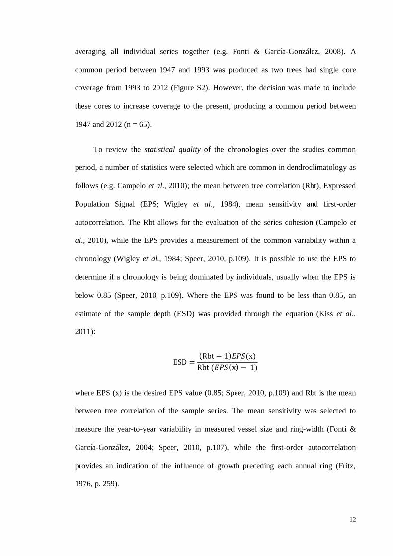
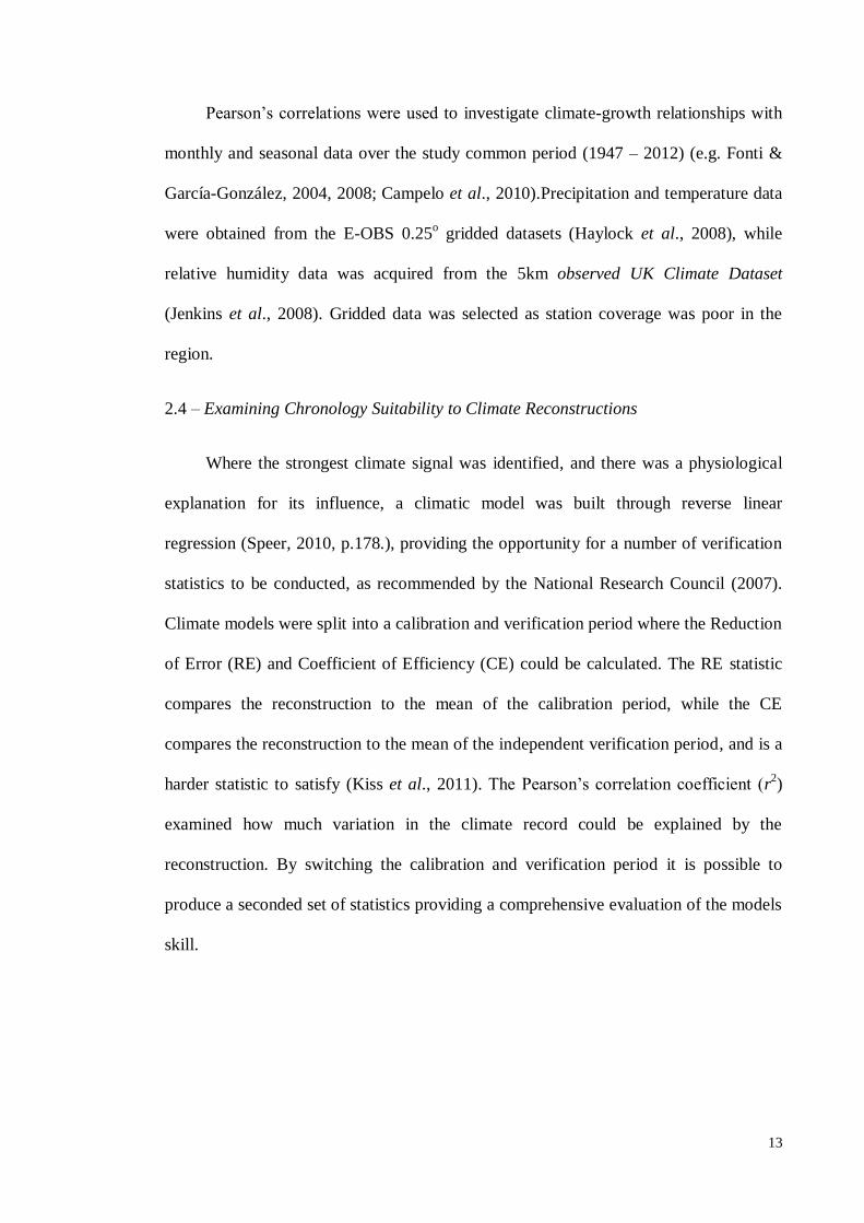
In total 43,950 earlywood vessels were measured, and it can be seen in Figure 3.1

that the frequency distribution of vessel area was skewed towards the smaller vessel

sizes. Vessel area ranged between 10,001 μm2 and 164,266 μm

2 with a mean and

median of 50,130 μm2 and

48,245 μm

2 respectively.

3.2 – Chronology Analysis

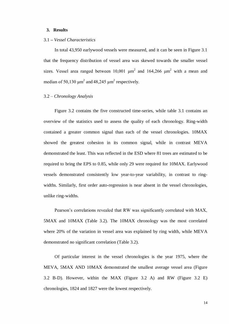
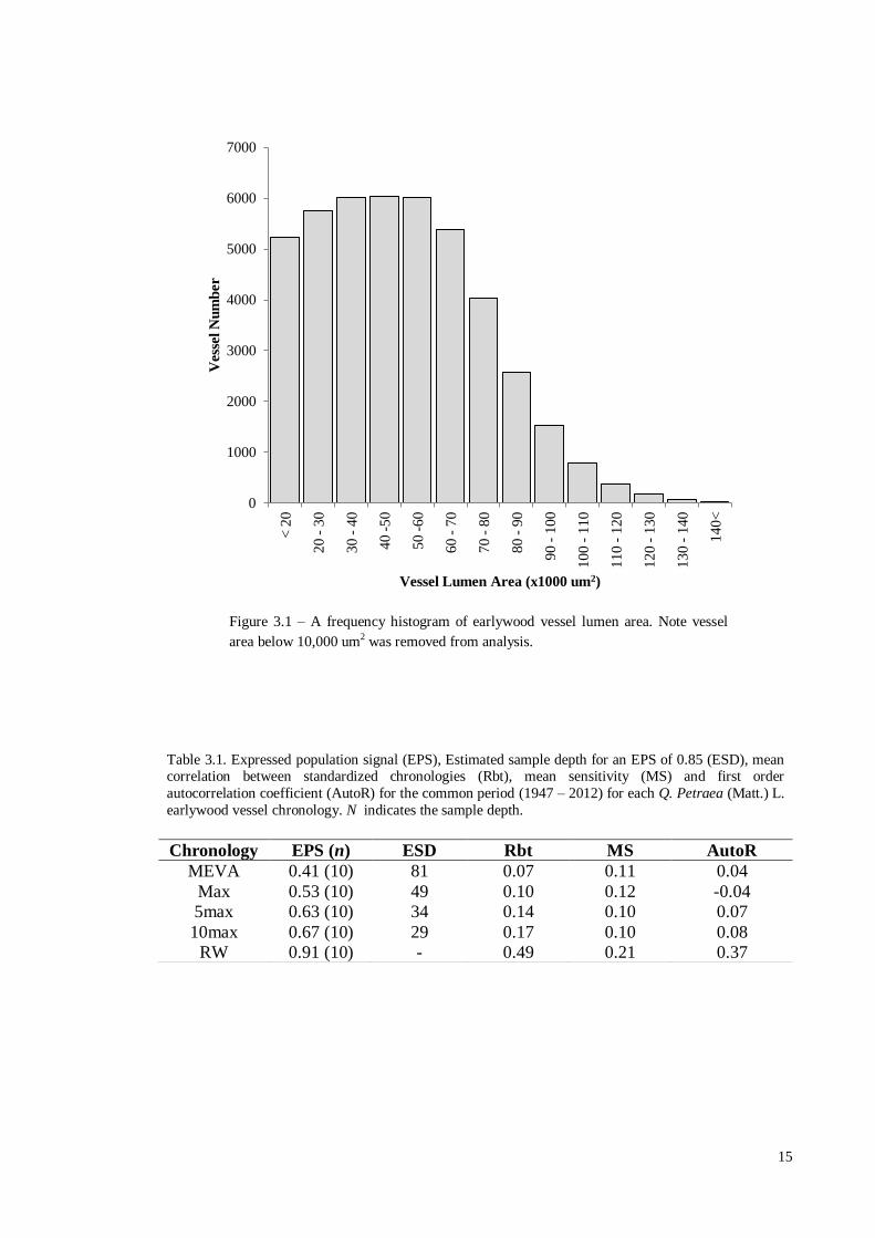
Figure 3.2 contains the five constructed time-series, while table 3.1 contains an

overview of the statistics used to assess the quality of each chronology. Ring-width

contained a greater common signal than each of the vessel chronologies. 10MAX

showed the greatest cohesion in its common signal, while in contrast MEVA

demonstrated the least. This was reflected in the ESD where 81 trees are estimated to be

required to bring the EPS to 0.85, while only 29 were required for 10MAX. Earlywood

vessels demonstrated consistently low year-to-year variability, in contrast to ring-

widths. Similarly, first order auto-regression is near absent in the vessel chronologies,

unlike ring-widths.

Pearson’s correlations revealed that RW was significantly correlated with MAX,

5MAX and 10MAX (Table 3.2). The 10MAX chronology was the most correlated

where 20% of the variation in vessel area was explained by ring width, while MEVA

demonstrated no significant correlation (Table 3.2).

Of particular interest in the vessel chronologies is the year 1975, where the

MEVA, 5MAX AND 10MAX demonstrated the smallest average vessel area (Figure

3.2 B-D). However, within the MAX (Figure 3.2 A) and RW (Figure 3.2 E)

chronologies, 1824 and 1827 were the lowest respectively.

15

0

1000

2000

3000

4000

5000

6000

7000

< 2

0

20 -

30

30 -

40

40

-5

0

50

-6

0

60

- 7

0

70

- 8

0

80

- 9

0

90

- 1

00

10

0 -

11

0

11

0 -

12

0

12

0 -

13

0

13

0 -

14

0

14

0<

Vess

el N

um

ber

Vessel Lumen Area (x1000 um2)

Table 3.1. Expressed population signal (EPS), Estimated sample depth for an EPS of 0.85 (ESD), mean correlation between standardized chronologies (Rbt), mean sensitivity (MS) and first order

autocorrelation coefficient (AutoR) for the common period (1947 – 2012) for each Q. Petraea (Matt.) L.

earlywood vessel chronology. N indicates the sample depth.

Chronology EPS (n) ESD Rbt MS AutoR

MEVA 0.41 (10) 81 0.07 0.11 0.04

Max 0.53 (10) 49 0.10 0.12 -0.04

5max 0.63 (10) 34 0.14 0.10 0.07

10max 0.67 (10) 29 0.17 0.10 0.08

RW 0.91 (10) - 0.49 0.21 0.37

Figure 3.1 – A frequency histogram of earlywood vessel lumen area. Note vessel

area below 10,000 um2 was removed from analysis.

16

0.5

0.7

0.9

1.1

1.3

1.5

1.7

1860 1880 1900 1920 1940 1960 1980 2000

A.

0.3

0.5

0.7

0.9

1.1

1.3

1.5

B.

0.3

0.5

0.7

0.9

1.1

1.3

1.5

C.

0.5

0.7

0.9

1.1

1.3

1.5

D.

0.4

0.9

1.4

1.9

E.

2

6

10

1860 1880 1900 1920 1940 1960 1980 2000

F.

Gro

wth

In

dex

Year

Figure 3.2 – Earlywood vessel and ring-width index chronologies: A) MAX, B) 5MAX, C) 10MAX, D)

MEVA and E) RW for the period 1860 - 2012. Grey lines represent individual series and red is the average

chronology. F) Illustrates the sample depth. Note truncated axis.

17

3.3 – Climate-Growth Relationships

Figure 3.3 provides an overview of the climate-growth correlations of

precipitation and temperature (1951 – 2012, n = 61), as well as humidity (1961 – 2011,

n = 50). Precipitation was weakly correlated with each vessel chronology throughout the

year, but the majority were non-significant. The highest vessel / precipitation

correlations were seen between MEVA and August as well as MAX and spring (March,

April and May), with both demonstrating a Pearson’s correlation of 0.30 (p<0.05). RW

demonstrated a weak spring precipitation signal (r = 0.08, p>0.05) due to a contrasting

relationship with April (r = 0.28, p<0.05) and May (r = -0.29, p<0.05). June saw a

return of a positive correlation (r = 0.27, p<0.05), which was reflected in the summer

(June, July & August) relationship (r = 0.28, p<0.05). Annual temperatures were on the

whole negatively correlated with earlywood vessel area. The strongest temperature

correlation was between August and 10MAX (r = -0.44, p<0.01), however the

relationship, although weaker, was evident in MAX, 5MAX and MEVA (Figure S3).

Vessel area was also significantly correlated with previous December’s temperature

which was most evident in 10MAX (r = -0.34, p<0.01). However, the relationship was

much weaker in MEVA (r = -0.20, p>0.05). RW’s strongest relationship was with

January temperatures (r = -0.40, p<0.01). In addition, there was a significant correlation

with May temperature (r = 0.30, p<0.05), while the relationship seen between vessel

area and August was weaker in the RW chronology (r = -0.21, p>0.05). The strongest

correlation with the climate data and the vessel chronologies was between March

Table 3.2 – Pearson’s correlations and in brackets r2 values between earlywood vessel and the ring-

width chronologies for the study common period (1947 – 2012).

Chronology MAX ( r2) 5MAX( r

2) 10MAX( r

2) MEVA( r

2)

RW 0.39**(0.15) 0.43**(0.18) 0.45**(0.20) 0.16(0.03) ** correlation significant at 0.01

18

Figure 3.3 – Climate-growth correlations between precipitation, temperature, humidity (overleaf)

and the constructed chronologies. Blue = MAX; Red = 5MAX; Green = 10MAX; Purple = MEVA

and Orange = RW. Solid lines – p<0.05; Dashed lines – p<0.01

-0.50

-0.30

-0.10

0.10

0.30

0.50

(-)

Au

g

(-)S

ep

(-)O

ct

(-)N

ov

(-)D

ec

Jan

Feb

Mar

Apr

May

Jun

Jul

Au

g

Au

tum

n

Win

ter

Spri

ng

Su

mm

er

-0.50

-0.30

-0.10

0.10

0.30

0.50

(-)

Au

g

(-)S

ep

(-)O

ct

(-)N

ov

(-)D

ec

Jan

Feb

Mar

Apr

May

Jun

Jul

Au

g

Au

tum

n

Win

ter

Spri

ng

Su

mm

er

-0.50

-0.30

-0.10

0.10

0.30

0.50

(-)

Au

g

(-)S

ep

(-)O

ct

(-)N

ov

(-)D

ec

Jan

Feb

Mar

Apr

May

Jun

Jul

Au

g

Au

tum

n

Win

ter

Spri

ng

Su

mm

er

-0.50

-0.30

-0.10

0.10

0.30

0.50

(-)

Au

g

(-)S

ep

(-)O

ct

(-)N

ov

(-)D

ec

Jan

Feb

Mar

Apr

May

Jun

Jul

Au

g

Au

tum

n

Win

ter

Spri

ng

Su

mm

er

-0.50

-0.30

-0.10

0.10

0.30

0.50

(-)

Au

g

(-)S

ep

(-)O

ct

(-)N

ov

(-)D

ec

Jan

Feb

Mar

Apr

May

Jun

Jul

Au

g

Au

tum

n

Win

ter

Spri

ng

Su

mm

er

-0.50

-0.30

-0.10

0.10

0.30

0.50

(-)

Au

g

(-)S

ep

(-)O

ct

(-)N

ov

(-)D

ec

Jan

Feb

Mar

Apr

May

Jun

Jul

Au

g

Au

tum

n

Win

ter

Spri

ng

Su

mm

er

-0.50

-0.30

-0.10

0.10

0.30

0.50

(-)

Au

g

(-)S

ep

(-)O

ct

(-)N

ov

(-)D

ec

Jan

Feb

Mar

Apr

May

Jun

Jul

Au

g

Au

tum

n

Win

ter

Spri

ng

Su

mm

er

-0.50

-0.30

-0.10

0.10

0.30

0.50

(-)

Au

g

(-)S

ep

(-)O

ct

(-)N

ov

(-)D

ec

Jan

Feb

Mar

Apr

May

Jun

Jul

Au

g

Au

tum

n

Win

ter

Spri

ng

Su

mm

er

-0.50

-0.30

-0.10

0.10

0.30

0.50

(-)

Au

g

(-)S

ep

(-)O

ct

(-)N

ov

(-)D

ec

Jan

Feb

Mar

Apr

May

Jun

Jul

Au

g

Au

tum

n

Win

ter

Spri

ng

Su

mm

er

-0.50

-0.30

-0.10

0.10

0.30

0.50

(-)

Au

g

(-)S

ep

(-)O

ct

(-)N

ov

(-)D

ec

Jan

Feb

Mar

Apr

May

Jun

Jul

Au

g

Au

tum

n

Win

ter

Spri

ng

Su

mm

er

Precipitation Temperature

Corr

elati

on

19

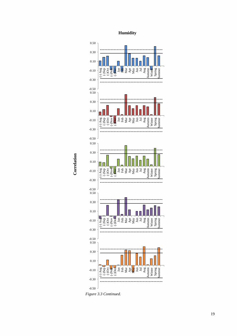
Figure 3.3 Continued.

-0.50

-0.30

-0.10

0.10

0.30

0.50

(-)

Au

g

(-)S

ep

(-)O

ct

(-)N

ov

(-)D

ec

Jan

Feb

Mar

Apr

May

Jun

Jul

Au

g

Au

tum

n

Win

ter

Spri

ng

Su

mm

er

-0.50

-0.30

-0.10

0.10

0.30

0.50

(-)

Au

g

(-)S

ep

(-)O

ct

(-)N

ov

(-)D

ec

Jan

Feb

Mar

Apr

May

Jun

Jul

Au

g

Au

tum

n

Win

ter

Spri

ng

Su

mm

er

-0.50

-0.30

-0.10

0.10

0.30

0.50

(-)

Au

g

(-)S

ep

(-)O

ct

(-)N

ov

(-)D

ec

Jan

Feb

Mar

Apr

May

Jun

Jul

Au

g

Au

tum

n

Win

ter

Spri

ng

Su

mm

er

-0.50

-0.30

-0.10

0.10

0.30

0.50

(-)

Au

g

(-)S

ep

(-)O

ct

(-)N

ov

(-)D

ec

Jan

Feb

Mar

Apr

May

Jun

Jul

Au

g

Au

tum

n

Win

ter

Spri

ng

Su

mm

er

-0.50

-0.30

-0.10

0.10

0.30

0.50

(-)

Au

g

(-)S

ep

(-)O

ct

(-)N

ov

(-)D

ec

Jan

Feb

Mar

Apr

May

Jun

Jul

Au

g

Au

tum

n

Win

ter

Spri

ng

Su

mm

er

Humidity

Corr

elati

on

20

relative humidity and 5MAX (r = 0.46, p<0.01), and although weaker, was present in

each vessel chronology (Figure 3.3). This trend was reflected in the significant

correlation with spring relative humidity (apart from MEVA). RW also demonstrated a

significant correlation with March relative humidity, however this was weaker than the

vessel chronologies (r = 0.34, p<0.05). RW’s strongest correlation with relative

humidity was seen in August (r = 0.40, p<0.01), which was reflected by the correlation

with average summer relative humidity (r = 0.41, p<0.01).

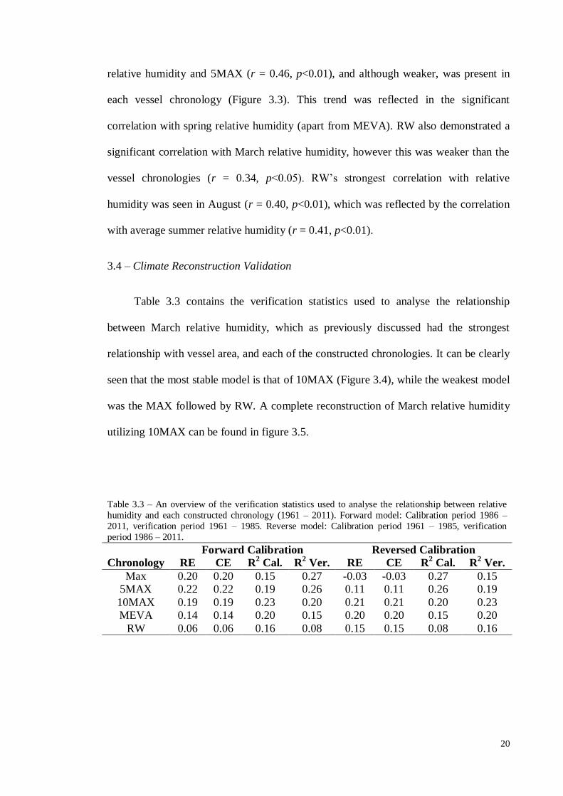
3.4 – Climate Reconstruction Validation

Table 3.3 contains the verification statistics used to analyse the relationship

between March relative humidity, which as previously discussed had the strongest

relationship with vessel area, and each of the constructed chronologies. It can be clearly

seen that the most stable model is that of 10MAX (Figure 3.4), while the weakest model

was the MAX followed by RW. A complete reconstruction of March relative humidity

utilizing 10MAX can be found in figure 3.5.

Table 3.3 – An overview of the verification statistics used to analyse the relationship between relative

humidity and each constructed chronology (1961 – 2011). Forward model: Calibration period 1986 –

2011, verification period 1961 – 1985. Reverse model: Calibration period 1961 – 1985, verification

period 1986 – 2011.

Forward Calibration Reversed Calibration

Chronology RE CE R2 Cal. R

2 Ver. RE CE R

2 Cal. R

2 Ver.

Max 0.20 0.20 0.15 0.27 -0.03 -0.03 0.27 0.15

5MAX 0.22 0.22 0.19 0.26 0.11 0.11 0.26 0.19

10MAX 0.19 0.19 0.23 0.20 0.21 0.21 0.20 0.23

MEVA 0.14 0.14 0.20 0.15 0.20 0.20 0.15 0.20

RW 0.06 0.06 0.16 0.08 0.15 0.15 0.08 0.16

21

4. Discussion

For a successful and accurate climate reconstruction to be produced from tree

based proxies, it is imperative that there is a strong common signal between individuals

(Fonti & García-González, 2008). Ring-width series clearly demonstrated shared

variability, while vessel chronologies were weaker. In fact, this is recurrent within the

literature (e.g. García-González & Eckstein, 2003; Fonti & García-González, 2004;

Tardiff & Conciatori, 2006; Fonti & García-González, 2008; Campelo et al., 2010).

Explanations are speculative, however, it has been suggested that earlywood vessels are

more strongly influenced by internal biological controls than external factors

(Woodcock, 1989; Fonti & García-González, 2004; Eilmanm et al., 2006). In fact, this

is reflected by the difference between the RW and vessel chronologies mean sensitivity,

where the vessel chronologies could be considered as complacent (Speer, 2010, p.107.).

The fact that there appears to be an internal control of earlywood vessel area is not

surprising. It has been found that within Q. petraea (Matt.) L., frost induced embolism

each winter, reduces conductivity within the earlywood vessels that were formed that

spring (Hacke & Sauter, 1996; Fonti et al., 2009). Earlywood vessels are important in

ring-porous oaks, as they have been found to provide up to 95% of annual hydraulic

conductivity (Cocuera et al., 2006; Alla & Camarero, 2012). Thus each spring, prior

bud-burst and leaf development, there must be an emphasis within ring-porous species

to produce large earlywood vessels to ensure sufficient hydraulic conductivity (Breda &

Granier, 1996; Fonti et al., 2009; Alla & Camarero, 2012). However, it is likely that

there is also a biological constraint on the maximum size of vessel area, as larger vessels

are thought to be more prone to embolism (Ewers, 1985; Kongoh et al., 2006).

Consequently, it is hypothesised that the reduced common signal and mean sensitivity

compared to RW, is due to a biologically controlled constraint on vessel size.

22

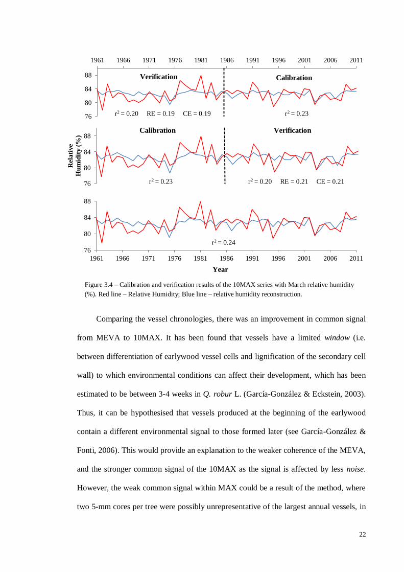
Comparing the vessel chronologies, there was an improvement in common signal

from MEVA to 10MAX. It has been found that vessels have a limited window (i.e.

between differentiation of earlywood vessel cells and lignification of the secondary cell

wall) to which environmental conditions can affect their development, which has been

estimated to be between 3-4 weeks in Q. robur L. (García-González & Eckstein, 2003).

Thus, it can be hypothesised that vessels produced at the beginning of the earlywood

contain a different environmental signal to those formed later (see García-González &

Fonti, 2006). This would provide an explanation to the weaker coherence of the MEVA,

and the stronger common signal of the 10MAX as the signal is affected by less noise.

However, the weak common signal within MAX could be a result of the method, where

two 5-mm cores per tree were possibly unrepresentative of the largest annual vessels, in

76

80

84

88

1961 1966 1971 1976 1981 1986 1991 1996 2001 2006 2011

Verification Calibration

r2 = 0.20 RE = 0.19 CE = 0.19 r2 = 0.23

76

80

84

88

1961 1966 1971 1976 1981 1986 1991 1996 2001 2006 2011

r2 = 0.24

76

80

84

88

Rela

tive

Hu

mid

ity (

%)

r2 = 0.20 RE = 0.21 CE = 0.21 r2 = 0.23

Verification Calibration

Figure 3.4 – Calibration and verification results of the 10MAX series with March relative humidity

(%). Red line – Relative Humidity; Blue line – relative humidity reconstruction.

Year

23

contrast to García-González & Fonti (2007). In fact, some investigations have taken

three cores per tree (e.g. García-González & Eckstein, 2003), although this hasn’t

necessarily been shown to be beneficial. It may be possible to improve the common

signal by increasing the sample size. Although this study predicted a large range of trees

that would be required to get an EPS of 0.85, the estimates are feasible as many dendro-

based reconstructions include hundreds of specimens (e.g. Grudd et al., 2002; Grudd,

2008; Cooper et al., 2013; Wilson et al., 2013).

For earlywood vessel area to be viewed as a useful climatic proxy, it must be

demonstrated that the signal it contains is unique, or better in respect to other ‘easier’ to

obtain tree proxies (Fonti & García-González, 2004). Although significantly correlated,

RW could only account for a small amount of variation within the earlywood vessel

chronologies. In addition, climate-growth models demonstrated differing responses.

Fonti & García-González (2008) suggest that the differences in response can be

attributed to how radial growth and vessels are affected by environmental stimuli. They

argue that radial increment is controlled by the sum of environmental and biological

processes over a year, while vessels are influenced by fewer controls, over a shorter

period of time. Thus, it can be said that at this location vessels and RW have responded

differently to climatic influences, which has been repeatedly demonstrated at different

locations in the literature (e.g. Pumijumnong & Park, 1999; Fonti & García-González,

2004; Matisons & Brumelis, 2012). Consequently, there appears to be merit in

researching the climatic content of earlywood vessel area at this location.

Due to the short period in which individual vessels can be influenced by

environmental factors (see above), it is hypothesised that they contain a high resolution

climatic signal (Eckstein, 2004). This was reflected by the vessels being most strongly

correlated with March humidity. The response to humidity, although a first in the

24

70

75

80

85

90

95

1860 1880 1900 1920 1940 1960 1980 2000

Rela

tive H

um

idit

y (

%)

Year

Figure 3.5 – Reconstruction of past March relative humidity (%) for the period 1860 – 2011 for the National Botanic Gardens of Wales produced from the 10MAX

series. The black line represents the reconstruction, while the red line is the observed relative humidity (see Jenkins et al., 2008). Grey lines represent the

uncertainty of the reconstruction utilizing Gaussian error propagation (±95%).

24

25

literature, is not surprising as vessel area is thought to be linked to moisture availability

(e.g. Knigge & Schulz, 1961; Pumijumnong & Park, 1999; García-González &

Eckstein, 2003; Corcuera et al., 2004; Fonti & García-González, 2004; Eilmann et al.,

2006). In fact, vessel area has been observed to be greater in humid than drier climates

(Kondoh et al., 2006). Thus, it is hypothesised that as relative humidity increases, so

does the moisture availability within the soil, due to precipitation and reduced

evaporation. With an increase in soil moisture content, the tree root system can take

advantage. As water quantities increase within the trees hydrosystem, turgor pressure,

which plays a large role in determining cell size, will increase (Ray et al., 1972; Boyer,

1985; Eilmann et al., 2006). Ultimately, this explains the relationship observed. The fact

that this signal was strongest in relation to March relative humidity can be explained

physiologically. Within ring-porous oak, the largest vessels are produced at the

beginning of the growing season, prior bud burst, ensuring adequate hydraulic

conductivity. Phenological observations have found that within South Wales the first-

flush begins early in the growing season, at the end of March and beginning of April

(Forestry Commission, 2001). Thus, the largest vessels would be expected to respond to

environmental stimuli during March. However, it could then be argued that the MAX

chronology should have contained the strongest response, but it is possible that an

under-representation of the largest vessels influenced the result, which is suggested by

the weak statistical quality of the chronology. In fact, it has previously been suggested

that selecting the largest vessels would not provide an optimal signal (García-González

& Fonti, 2006). To confirm these observations, more local phenological investigations

in conjunction with the extraction of micro-cores to investigate vessel development are

required (e.g. Fonti et al., 2007).

26

The highly significant correlation between August temperatures and the vessel

chronologies is harder to explain, as earlywood production is likely to have ceased prior

this point (Speer, 2010. P.43.). However, earlywood and latewood production is

dependent on environmental conditions and it is possible that earlywood production

could extend late into the summer months (Speer, 2010. P.43.). In fact, this explanation

could have some potential as the inclusion of the smaller vessels, which can be assumed

to be produced later in the year (García-González & Fonti, 2006), improved the signal

strength. In addition, it has been documented that cooler conditions slow cell formation

resulting in a longer window in which the climate can affect vessel characteristics (i.e.

Fonti & García-González, 2004) although, such an influence in the summer months is

questionable. Assuming, earlywood production had ceased prior this point other

explanations would be required. For instance, the August temperature signal could have

arisen due to its influence on earlier formed vessels, which would explain why the

MAX and 5MAX chronologies also demonstrated a significant correlation. However,

observations imply that cell wall lignification, after 3-4 weeks, inhibits alteration of

vessel characteristics (Eckstein, 2004). Although evidence suggests that August

temperature is influencing vessel area, it would be wrong to conclude this without

further research, as correlation does not mean causation devoid of a clear physiological

mechanism.

Results demonstrated that vessel chronologies were less dependent on previous

year conditions compared to RW. This has been reported within the literature (e.g.

García-González & Eckstein, 2003). In fact, it appears to be one of the advantages of

vessel chronologies over ring-width chronologies. However, significant correlations

with previous winter temperatures were found. Within oak it has been repeatedly

observed that ring-width is negatively related to winter temperatures (Pilcher, 1995) and

27

it can be expected that vessels are influenced by the same factors. It has been suggested

that this signal is a result of winter conditions affecting the storage and synthesis of

carbohydrates, which in turn influences the coming spring growth (Aloni, 1991; Alla &

Camarero, 2012). However, in contrast to Fonti & García-González (2004) no influence

was found with previous summer conditions.

Examination of the RE, CE and correlation statistics demonstrated that the climate

models varied in their reconstruction skill. The 5MAX chronology was found to have

the strongest correlation with the humidity record however, considering the RE, CE and

r2

statistics, it was found that the climate model was unsuitable. On the other hand, the

10MAX chronology was found to be more stable in its predictive ability. A possible

explanation is that chronologies constructed from the largest or five largest vessels

could be subject to greater errors in measurement, due to the use of only a select few

vessels. Again, it is also possible that relying on a small selection of vessels from just

two 5-mm cores may result in large vessels being missed, leading to an under-estimate

of annual vessel size. Thus, the 10MAX may overcome these limitations by including

more vessels (without mixing climatic signals), thus a greater chance of gaining an

adequate vessel sample, representing different vessel sizes. Although, the validation

statistics suggest the 10MAX chronology is suitable for a climatic reconstruction, it is

important to remember that the signal strength between series is not satisfactory, thus

the reconstruction could be miss-leading. The reconstruction predicted that March 1975

was the least humid of the study period, in contrast to the observed humidity data.

Although this raises question marks as to the suitability of the reconstruction, it is

interesting to note that between 1975 and 1976 Western Europe saw some of the worst

drought conditions on record (Fleig et al., 2011). Although, the drought is considered to

have begun late in the spring (Ratcliffe, 1978), there had been a period from 1970 to

28

1974 of dry winters which lead to depleted ground water levels in the spring of 1975

(Ratcliffe, 1978). As vessel size is part dependent on moisture availability during spring

(Ray et al., 1972; Boyer, 1985; Eilmann et al., 2006) it is suggest here, that the reduced

vessel sizes of 1975 seen in the reconstruction, and in a number of the raw chronologies,

is a consequence of these dry conditions. This result conforms to ideas that vessels

provide a potential proxy for extreme climatic years (e.g. Knigge & Schulz, 1961).

When considering the previous discussion a number of limitations should be

considered. The humidity data set that was utilized was relatively short, thus increasing

the risk of spurious results. In addition, there is no detailed phenological data available

concerning vessel formation and leaf flushing at the research location, which would aid

in data interpretation.

Following the previous discussion it is possible to evaluate the use of vessel area

chronologies as a climate proxy within the UK. In line with other European studies,

there does appear to be a climatic signal contained within vessel area increments which

was distinct, and in some cases, stronger than ring-width measurements at the research

location in question. In addition, there does seem to be potential in the use of vessel area

chronologies in producing very high resolution reconstructions, which will benefit in

our understanding of the climate system. The prospect of vessels recording a humidity

signal is advantageous in examining climate change, past and present, as humidity plays

a major role in the energy balance of the climate system (Shu et al., 2005). However, it

is clear that the quality of the constructed chronologies is something that needs to be

questioned, although this maybe improved through larger sample sizes. Finally, it has

been demonstrated that care and knowledge must be used when utilizing vessels in a

reconstruction, as the strongest correlation may not be the best, and the use of statistics

such as the RE and CE is strongly recommended.

29

Although the results of this investigation have demonstrated the potential use of

vessels as a proxy, the field is still relatively new and further work is required. Much

has now been published on the climatic influences on vessel area, however, there are

conflicting results. Thus, further investigation on the climatic influence, site conditions

and differences between species on vessel area is required. Great benefit will also be

obtained if such investigations occur in new regions as spatially, present studies are

limited (e.g. Latvia, Matisons et al., 2013; Switzerland, Fonti & Garcia-González,

2004). In addition, it can be argued that the science needs to advance, and work should

now begin to focus on producing actual climatic reconstructions utilizing statistics such

as the RE and CE. Ultimately, this will provide a greater understanding of the suitability

of vessel area as a proxy. As many of the longest tree-ring chronologies utilize

preserved wood samples, research is required to examine the suitability of vessels from

such media, and if results are positive, there is potential that long vessel chronologies

could be built from existing samples (e.g. Friedrich et al., 2007). Finally, there is the

future possibility that if techniques are developed which allow the accurate

identification of when specific vessels were formed, that high resolution reconstructions

of the growing season maybe produced from the same core samples, providing an

invaluable source of past climatic information.

30

5. Conclusion

High resolution proxies are highly sort after within paleo-climatology, and

earlywood vessel area chronologies are thought to be a promising avenue. This thesis

aimed to investigate the applicability of earlywood vessel area as a proxy, and was a

first in the United Kingdom. From this investigation a number of conclusions can be

drawn:

1) It appears that time-series of vessel areas have a reduced statistical quality

compared to ring-width chronologies, in respect to their common signal and

variability. In addition, vessels demonstrated a reduced year to year sensitivity to

environmental stimuli. However, vessel series had the advantage of being less

dependent on previous year growth than RW.

2) Annually, earlywood vessels at this location were mainly influenced by March

relative humidity. In addition, August temperatures appeared to be negatively

related to the vessel series, although there is no clear mechanism to explain this

relationship. Vessel chronologies displayed different responses to the climate

compared to a ring-width series, suggesting there is merit in the use of vessel

area chronologies at this location.

3) A chronology constructed from the average area of all earlywood vessels

demonstrated a weaker correlation to the climate, compared to chronologies

composed of selected vessel sizes, demonstrating that different groups of vessels

may contain different environmental signals. The average of the 5 largest vessels

were most related to March relative humidity, compared to the other series,

while a series composed of the largest ten vessels was more related to August

temperatures.

31

4) Although this study produced a relative humidity reconstruction, caution is

needed in interpreting the results due to weak verification statistics. However,

there is an indication of vessels containing a record of extreme events. A larger

sample depth would probably have improved the expressed climate signal. Thus,

it would appear to be potential in using vessels as a proxy within the UK.

From this study a number areas for further research have been identified. Most

importantly is the need to conduct similar research with different species, in new

regions and climates, to understand differences in vessel responses, while, further

insight into vessel development in relation to phenological observations would also be

beneficial. In addition, emphasis should be placed on examining new methods to

identify the signals contained within specific vessel groups, which could lead to the

future possibility of an unprecedented high resolution climate proxy.

32

References

Alla, A. Q., & Camarero, J. J. (2012) “Contrasting responses of radial growth and wood

anatomy to climate in a Mediterranean ring-porous oak: implications for its

future persistence or why the variance matters more than the mean” European

Journal of Forest Research. 131. 1537 – 1550.

Allan, R. P., & Soden, B. J. (2008) “Atmospheric warming and the amplification of

precipitation” Science. 321. Pp. 1481 – 1484.

Aloni, R. (1991) Wood formation in deciduous hardwood trees. In: A. S. Raghavendra,

ed. (1991) Physiology of Trees. New York: Wiley. Pp. 75 – 197.

Astrade, L., & Bégin, Y. (1997) “Tree-ring response of Populus tremula L. and Quercus

robur L. to recent spring flodds of the Saone River, France” Ecoscience. 4. 232

– 239.

Barber, K. E., Chambers, F. M., Maddy, D., Stoneman, R., & Brew, J. S. (1994) “A

sensitive high-resolution record of late Holocene climate change from a raised

bog in northern England” The Holocene. 4. 198 – 205.

Bellard, C., Bertelsmeier, C., Leadley, P., Thuiller, W., & Courchamp, F. (2012)

“Impacts of climate change on the future of biodiversity” Ecology letters. 15.

365 – 377.

Boyer, J. S. (1985) “Water transport” Annual Review of Plant Physiology and Plant

Molecular Biology. 36. 473 – 516.

Breda, N., & Granier, A. (1996) “Intra- and interannual variations of transpiration, leaf

area index and radial growth of a sessile oak stand (Quercus petraea)” Annals

of Forest Science. 53. 521 – 536.

Briffa, K. R., Jones, P. D., & Schweingruber, F. H. (1988) “Summer temperature

patterns over Europe: A reconstruction from 1750 A.D. based on maximum

latewood density indices of conifers” Quaternary Research. 30. 36 – 52.

Brunstein, C. F. (1996) “Climatic significance of the bristlecone pine latewood frost-

ring record at Almagre Mountain, Colorado, USA” Arctic and Alpine

Research. 28. 65 – 76.

Burk, R. L., & Stuiver, M. (1981) “Oxygen isotope ratios in trees reflect mean annual

temperature and humidity” Science. 211. 1417 – 1419.

Campelo, F. (2012) detrendeR: Start the detrendeR Graphical User Interface (GUI). R

Package version 1.0.4. Available at: < http://CRAN.R-

project.org/package=detrendeR > [Accessed 1/9/13].

Campelo, F., Gutiérrez, E., Ribas, M., Nabais, C., & Freitas, H. (2007) “Relationships

between climate and double rings in Quercus ilex from NE Spain” Canadian

Journal of Forest Research. 37. 1915 – 1923.

33

Campelo, F., Nabais, C., Gutiérrez, E., Freitas, H., & García-González, I. (2010)

“Vessel features of Quercus iles L. Growing under Mediterranean climate have

a better climatic signal than tree-ring width” Trees. 24. 463 – 470.

Carlquist, S. (1988) Comparative wood anatomy, Systematic, ecological, and

evolutionary aspects of dicotyledon wood. Berlin: Springer.

Cooper, R. J., Melvin, T. M., Tyers, I., Wilson, R. J., & Briffa, K. R. (2013) “A tre-ring

reconstruction of East Anglian (UK) Hydroclimate variability over the last

millennium” Climate Dynamics. 40. 1019 – 1039.

Corcuera, L., Camarero, J. J., & Gil-Pelegrin, E. (2004) “Effects of a severe drought on

growth and wood anatomical properties of Quercus faginea” IAWA Journal.

25. 185 – 204.

Corcuera, L., Camarero, J. J., Sisó, S., & Gil-Pelegrin, E. (2006) “Radial-growth and

wood-anatomical changes in over aged Quercus pyrenaica coppice stands:

functional responses in a new Mediterranean landscape” Trees. 20. 91 – 98.

Coumou, D., & Rahmstorf, S. (2012) “A decade of weather extremes” Nature Climate

Change. 2, 7. 491 – 496.

DeSoto, L., Cruz, M. D. L., & Fonti, P. (2011) “Intra-annual patterns of tracheid size in

the Mediterranean tree Juniperus thurifera as an indicator of seasonal water

stress” Canadian Journal of Forest Research. 41. 1280 – 1294.

Eckstein, D. (2004) “Change in past environments – secrets of the tree hydrosystem”

New Phytologist. 163. 1 – 4.

Eckstein, D., Frisse, E., & Quiehl, F. (1977) “Holzanatomische Untersuchungen zum

Nachweis anthropogener Einflusse auf die Umweltbedingungen einer

Rotbuche” Angew. Bot. 51. 47-56.

Eilmann B., Weber, P., Rigling, A., & Eckstein, D. (2006) “Growth reactions of Pinus

sylvestris L. and Quercus pubescens Willd. to drought years at a xeric site in

Valais, Switzerland” Dendrochronologia. 23. 121 – 132.

Esper, J., Cook, E. R., & Schweingruber, F. H. (2002) “Low-frequency signals in long

tree-ring chronologies for reconstructing past temperature variability” Sciecne.

295. 2250 – 2253.

Esper, J., Krusic, P. J., Peters, K., & Frank, D. C. (2009) “Exploration of long-term

growth changes using the tree-ring program “Spotty”” Dendrochronologia. 27.

75 – 82.

Esper, J., Wilson, R. J. S., Frank, D. C., Moberg, A., Wanner, H., & Luterbacher, J.

(2005) “Climate: past ranges and future changes” Quaternary Science Reviews.

24. 2164 – 2166.

34

Ewers, F. W. (1985) “Xylem structure and water conduction in conifer trees, dicot trees,

and lianas” Int. Assoc. Wood Anat. Bull. 6. 309 – 317.

Fleig, A. K., Tallaksen, L. M., Hisdal, H., & Hannah, D. M. (2011) “Regional

hydrological drought in north-western Europe: linking a new regional drought

index with weather types” Hydrological Processes. 25. 1163 – 1179.

Fonti, P., & García-González, I. (2004) “Suitability of chestnut earlywood vessel

chronologies for ecological studies” New Phytologist. 163. 77 – 86.

Fonti, P., & García-González, I. (2008) “Earlywood vessel size of oak as a potential

proxy for spring precipitation in mesic sites” Journal of Biogeography. 35.

2249 – 2257.

Fonti, P., Solomonoff, N., & García-González, I. (2007) “Earlywood vessels of

Castanea sativa recored temperature before their formation” New Phytologist.

173. 562 – 570.

Fonti, P., Treydte, K., Osenstetter, S., Frank, D., & Esper, J. (2009) “Frequency-

dependent signals in multi-centennial oak vessel data” Palaeogeography,

Palaeoclimatology, Palaeoecology. 275. 92 – 99.

Forestry Commission (2001) Tree Phenology. [Online] Available at: <

http://www.forestry.gov.uk/images/cchg_oak_budburst_map.gif/$file/cchg_oa

k_budburst_map.gif >. [Accessed: 08/10/2013].

Friedrich, M., Remmele, S., Kromer, B., Hofmann, J., Spurk, M., Kaiser, K. F., Orcel,

C., & Kuppers, M. (2007) “The 12,460-year Hohenheim oak and pine tree-ring

chronology from Central Europe; a unique record for radiocarbon calibration

and paleoenvironment reconstructions” Radiocarbon. 46. 1111 -1122.

Fritts, H. C. (1976) Tree rings and climate. London: Academic Press.

Fritz, S. C., Juggins, S., Battarbee, R. W., & Engstrom, D. R. (1991) “Reconstruction of

past changes in salinity and climate using a diatom-based transfer function”

Nature. 352. 706 – 708.

García-González, I. G., & Eckstein, D. (2003) “Climatic signal of earlywood vessels of

oak on a maritime site” Tree Physiology. 23. 497 – 504.

García-González, I., & Fonti, P. (2006) “Selecting earlywood vessels to maximize their

environmental signal” Tree Physiology. 26. 1289 – 1296.

García-González, I., & Fonti, P. (2007) “Ensuring a representative sample of earlywood

vessels for dendroecological studies: an example from two ring-porous

species” Trees. 22. 237 – 244.

Grudd, H. (2008) “Tornetrask tree-ring width and density AD 500-2004: a test of

climatic sensitivity and a new 1500-year reconstruction of north Fennoscandian

summers” Climate Dynamics. 31. 843 – 857.

35

Grudd, H., Briffa, K. R., Karlen, W., Bartholin, T. S., Jones, P. D., & Kromer, B. (2002)

“A 7400-year tree-ring chronology in northern Swedish Lapland: natural

climatic variability expressed on annual to millennial timescales” The

Holocene. 12. 657 – 665.

Hacke, U., & Sauter, J. J. (1996) “Xylem dysfunction during winter and recovery of

hydraulic conductivity in diffuse-porous and ring-porous trees” Oecologia.

105. 435 – 439.

Haylock, M. R., Hofstra, N., Klein Tank, A. M.G., Klok, E. J., Jones, P. D., & New, M.

(2008) “A European daily high-resolution gridded dataset of surface

temperature and precipitation” Journal of Geophysical Research

(Atmospheres) 113. D20119. DOI: 10.1029/2008JD10201.

Jenkins, G. J., Perry, M. C., & Prior, M. J. (2008) The climate of the United Kingdom

and recent trends. [pdf] Exeter: Met Office Hadley Center. Available at: <

http://www.ukcip.org.uk/wordpress/wp-content/PDFs/UKCP09_Trends.pdf >

[Accessed 25/09/13].

Kalela-Brundin, M. (1999) “Climatic information from tree-rings of Pinus sylvestris L.

and a reconstruction of summer temperature back to AD 1500 in

Femundsmarka, eastern Norway, using partial least squares regression (PLS)

analysis” The Holocene. 9. 59 – 77.

Kiss, A., Wilson, R., & Bariska, I. (2011) “An experimental 392-year documentary-

based multi-proxy (vine and grain) reconstruction of May-July temperatures

for Koszeg, West-Hungary” Int. J. Biometeorol. 55. 595 – 611.

Knigge, W., & Schulz, H. (1961) “Einfluss der Jahreswitterung 1959 auf die

Zellartenverteilung, Faserlange und Gefassweite verschiedener Holzarten”

Holz als Roh- und Werkstoff. 19. 293 – 303.

Kondoh, S., Yahata, H., Nakashizyka, T., & Kongoh, M. (2006) “Interspecific variation

in vessel size, growth and drought tolerance of broad-leaved trees in semi-arid

regions of Kenya” Tree Physiology. 26. 899 – 904.

Mann, M. E., Bradley, R. S., & Hughes, M. K. (1999) “Northern hemisphere

temperatures during the past millennium: inferences, uncertainties and

limitations” Geophysical Research Letters. 26. 759 – 762.

Matisons, R., & Brumelis, G. (2012) “Influence of climate on tree-ring and earlywood

vessel formation in Quercus robur in Latvia” Trees. 26. 1251 – 1266.

Matisons, R., Elferts, D., & Brumelis, G. (2012) “Changes in climatic signals of English

oak tree-ring width and cross-section area of earlywood vessels in Latvia

during the period 1900-2009” Forest Ecology and Management. 279. 34 – 44.

Matisons, R., Elferts, D., & Brumelis, G. (2013) “Pointer years in tree-ring width and

earlywood-vessel area time series of Quercus robur – relation with climate

factors near its northern distribution limit” Dendrochronologia. 31. 129 – 139.

36

McCarroll, D., & Loader, N. J. (2004) “Stable isotopes in tree rings” Quaternary

Science Reviews. 23. 771 – 801.

McCarroll, D., Loader, N. J., Jalkanen, R., Gagen, M. H., Grudd, H., Gunnarson, B. E.,

Kirchhefer, A. J., Friedrich, M., Linderholm, H. W., Lindholm, H. W.,

Boettger, T., Los, S., Remmele, S., Kononov, Y. M., Yamazaki, Y. H., Young,

G. H. F., & Zorita, E. (2013) “A 1200-year multiproxy record of tree growth

and summer temperature at the northern pine forest limit of Europe” The

Holocene. DOI: 10.1177/0959683612467483.

McMichael, A. J., Woodruff, R. E., & Hales, S. (2006) “Climate change and human

health: present and future risks” The Lancet. 367. 859 – 869.

Moberg, A., Sonechkin, D. M., Holmgren, K., Datsenko, N. M., & Karlén, W. (2005)

“Highly variable northern hemisphere temperatures reconstructed from low-

and high- resolution proxy data” Nature. 433. 613 – 617.

National Botanic Gardens of Wales (2013) Waun Las Grasslands. [online] Available at:

< http://www.gardenofwales.org.uk/science/waun-las-grasslands > [Accessed

03/10/2013.

National Research Council (2007) Surface Temperature Reconstructions for the Last

2,000 Years. National Academies Press: Washington, DC.

Panyushkina, I. P., Hughes, M. K., Vaganov, E. A., & Munro, M. A. R. (2003)

“Summer temperature in northeastern Siberia since 1642 reconstrcuted from

tracheid dimensions and cell numbers of Larix cajanderi”. Canadian Journal

of Forest Research. 33. 1905 – 1914.

Petit, J. R., Jouzel, J., Raynaud, D., Barkov, I., Barnola, J. M., Basile, I., Bender, M.,

Chappellaz, J., Davis, M., Delaygue, G., Delmotte, M., Kotylakov, V. M.,

Legrand, M., Lipenkov, V. Y., Lorius, C., Pepin, L., Ritz, C., Saltzman, E., &

Stievenard, M. (1999) “Climate and atmospheric history of the past 420,000

years from the Vostok ice core, Antarctica” Nature. 399. 429-436.

Pilcher, J. R. (1995) Biological consideration in the interpretation of stable isotope

ratios in oak tree-rings. In B. Frenzel (ed) Problems of stable isotopes in tree-

rings, lake sediments and peat-bogs as climatic evidence for the Holocene.

157-161.

Pumijumnong, N., & Park, W. K. (1999) “Vessel chronologies from teak in northern

Thailand and their climatic signals” IAWA Journal. 20. 285 – 294.

R Core Team (2013). R: A language and environment for statistical computing. R

Foundation for Statistical Computing, Vienna, Austria. Available at <

http://www.R-project.org/ > [Accessed 1/09/13].

Ratcliffe, R. A. S., Miles, M. K., Rydz, B., & Shaw, E. M. (1978) “Meteorological

aspects of the 1975 – 76 drought [and discussion]” Proceedings of the Royal

Society A. 363. 3 – 20.

37

Ray, P. M., Green, P. B., & Cleland, R. (1972) “Role of turgor in plant-cell growth”

Nature. 239. 163 – 164.

Rinn, F. (2003) TSAP-Win-time series analysis and presentation dendrochronology and

related applications. Heidelberg: Frank Rinn.

Rodwell, J. S. (1991) British Plant Communities. Volume 1. Woodlands and scrub.

London: Cambridge University Press.

Rodwell, J. S. (1992) British Plant Communities. Volume 3. Grassland and montane

communities. London: Cambridge University Press.

Ruddiman, W. F. (2008) Earth’s Climate, Past and Future. New York: W. H. Freeman.

Salinger, M. J., & Griffiths, G. M. (2001) “Trends in New Zealand daily temperature

and rainfall extremes” International Journal of Climatology. 21. 1437 – 1452.

Sass, U., & Eckstein, D. (1995) “The variability of vessel size in beech (Fagus sylvatica

L.) and its ecophysiological interpretation” Trees. 9. 247 – 252.

Schume, H., Grabner, M., & Eckmullner, O. (2004) “The influence of an altered

groundwater regime on vessel properties of hybrid poplar” Trees. 18. 184 –

194.

Schweingruber, F.H. (2001) Dendroökologische Holzanatomie. Bern: Paul Haupt.

Shu, Y., Feng, X., Gazis, C., Anderson, D., Faiia, A. M., Tang, K., & Ettl, G. J. (2005)

“Relative humidity recorded in tree rings: A study along a precipitation

gradient in the Olympic Mountains, Washington USA” Geochimica et

Cosmochimica Acta. 69. 791 – 799.

Solomon, S., D. Qin, M. Manning, R.B. Alley, T. Berntsen, N.L. Bindoff, Z. Chen, A.

Chidthaisong, J.M. Gregory, G.C. Hegerl, M. Heimann, B. Hewitson, B.J.

Hoskins, F. Joos, J. Jouzel, V. Kattsov, U. Lohmann, T. Matsuno, M. Molina,

N. Nicholls, J. Overpeck, G. Raga, V. Ramaswamy, J. Ren, M. Rusticucci, R.

Somerville, T.F. Stocker, P. Whetton, R.A. Wood and D. Wratt, 2007:

Technical Summary. In: Climate Change 2007: The Physical Science Basis.

Contribution of Working Group I to the Fourth Assessment Report of the

Intergovernmental Panel on Climate Change [Solomon, S., D. Qin, M.

Manning, Z. Chen, M. Marquis, K.B. Averyt, M. Tignor and H.L. Miller

(eds.)]. Cambridge University Press, Cambridge, United Kingdom and New

York, NY, USA.

Speer, J. H. (2010) Fundamentals of tree-ring research. Tucson: The University of

Arizona Press.

St. George, S. & Nielsen, E. (2003) “Palaeoflood records for the Red River, Manitoba,

Canada, derived from anatomical tree-ring signitures” The Holocene. 13. 547 –

555.

38

St. George, S., & Nielsen, E. (2000) “Signatures of high-magnitude 19th century floods

in Quercus macrocarpa tree rings along the Red River, Manitoba, Canada”

Geology. 28. 899 – 902.

St. George, S., Nielsen, E., Conciatori, F., & Tardif, J. (2002) “Trends in Quercis

macrocarpa vessel areas and their implications for tree-ring paleoflood studies”

Tree-Ring Research. 58. 3 – 10.

Sundberg, R., Mober, A., & Hind, A. (2012) “Statistical framework for the evaluation

of climate model simulations by use of climate proxy data from the last

millennium – Part 1: Theory” Climate of the Past. 8. 1339 – 1353.

Tardif, J. C., & Conciatori, F. (2006) Influence of climate on tree rings and vessel

features in red oak and white oak growing near their northern distribution limit,

southwestern Quebec, Canada. Canadian Journal for Forest Research. 36.

2317 – 2330.

Westra, S., Alexander, L. V., & Zwiers, F. W. (2013) “Global increasing trends in annual

maximum daily precipitation” Journal of Climate. 26. 3904 – 3918.

Wigley, T. M. L., Briffa, K. R., & Jones, P. D. (1984) “On the average value of

correlated time series, with applications in Dendroclimatology and

Hydrometeorology” Journal of Climate and Applied Meteorology. 23. 201 –

213.

Wilson, R., Miles, D., Loader, N. J., Melvin, T., Cunningham, L., Cooper, R., & Briffa,

K. (2013) “A millennial long March-July precipitation reconstruction from

southern-central England” Climate Dynamics. 40. 997 – 1017.

Woodcock, D. W. (1989) “Climate sensitivity of wood-anatomical features in a ring-

porous oak (Quercus macrocarpa)” Canadian Journal for Forest Research. 19.

639 – 644.

39

Supplementary Materials for

An Evaluation of the Climatic Signal within the

Earlywood Vessel Area of Quercus petraea (Matt.) Liebl.

Darren Davies (552192)

This Section includes:

Supplementary Materials and Methods

Figs. S1 to S3

Tables S1 to S2

Captions for databases S1 to S3

Other Supplementary Materials for this manuscript includes the following:

CD Content Database S1 to S5:

1. Site cross-dating statistics

2. Comparison between constructed master chronology and that of Pilcher et al.,

(1984)

3. Master Chronology

4. Raw Vessel Chronologies

5. Detrended Vessel Chronologies

40

Materials and Methods

Chronology Dating

Provided in Database S1 is the cross-dating statistics used to analyse the relationship

between the individual sample cores. Where the t-value Ballie-Pilcher (TVBP), produced

by TSAP (Rinn, 2003), was found to be greater than 3.5, a significant relationship was

assumed (Baillie & Pilcher, 1973). Where significant relationships were identified, visual

inspection of ring-width graphs were used to identify any possibility of missed rings from

the measurement stage. Once these criteria were satisfied, cores were added to the master

chronology which was produced by TSAP (Rinn, 2003). To confirm the accuracy of the

master chronology, it was cross-dated with the master chronology of Pilcher et al., (1984)

where the TVBP value was 7.9 (Database S2). Consequently, the master chronology

produced was thought to be accurate (Database S3). The constructed chronology was found

to cover the period of 1773 – 2012, however, due to a reduced coverage and time

constraints only the period of 1860 – 2012 was considered for further analysis.

Sample Preparation

Initial analysis of core samples was conducted without alteration of the cores sanded

surface. However, it was found that WinCELL PRO (ver. 2013) software (Régents

Instruments Inc., Québec, Canada) was unable to accurately identify and measure vessel

lumina correctly in their natural form (Figure S1A). Initially, vessels were cleared with

compressed air and in-filled with white chalk by hand, to see if there was an improvement,

however, results were not satisfactory (Figure S1B). Therefore, following a popular

approach in the literature (e.g. Fonti et al., 2007; Fonti & García-González, 2008; Alla &

Camarero, 2012) the wood matrix was coloured black with permanent marker, in addition

41

to completing the previous steps. To prohibit chalk falling out of the vessels a coating of

hairspray was applied. Altogether, these steps greatly improved the identification and

measurement of the vessel areas (Figure S1C).

Vessel Sorting Package

As there was no readymade software for sorting the measured vessels by size, a package

was created in Microsoft Excel (ver. 2007) using Visual Basic for Applications code. The

Macro used within the package works in a logical fashion by selecting the area of each

vessel, from each year, and sorting them in ascending order. Following this the code

separates, from the annual vessel area size list, a selection of the largest, five largest, ten

largest and all the vessel areas and where appropriate produces an average. This is repeated

for each year of the series producing the chronologies described in table 2.1.

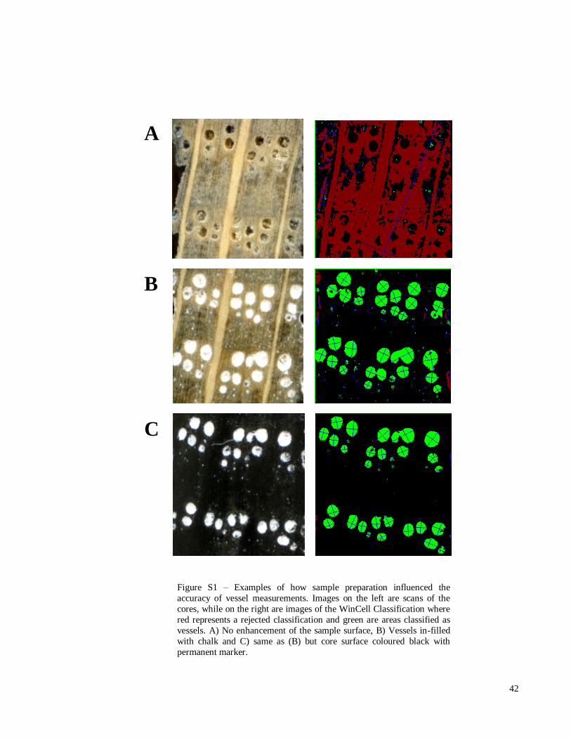
42

Figure S1 – Examples of how sample preparation influenced the

accuracy of vessel measurements. Images on the left are scans of the

cores, while on the right are images of the WinCell Classification where

red represents a rejected classification and green are areas classified as

vessels. A) No enhancement of the sample surface, B) Vessels in-filled

with chalk and C) same as (B) but core surface coloured black with

permanent marker.

A

B

C

43

Figure S2 – Sample coverage. Note NBGW007 and 014 are missing years.

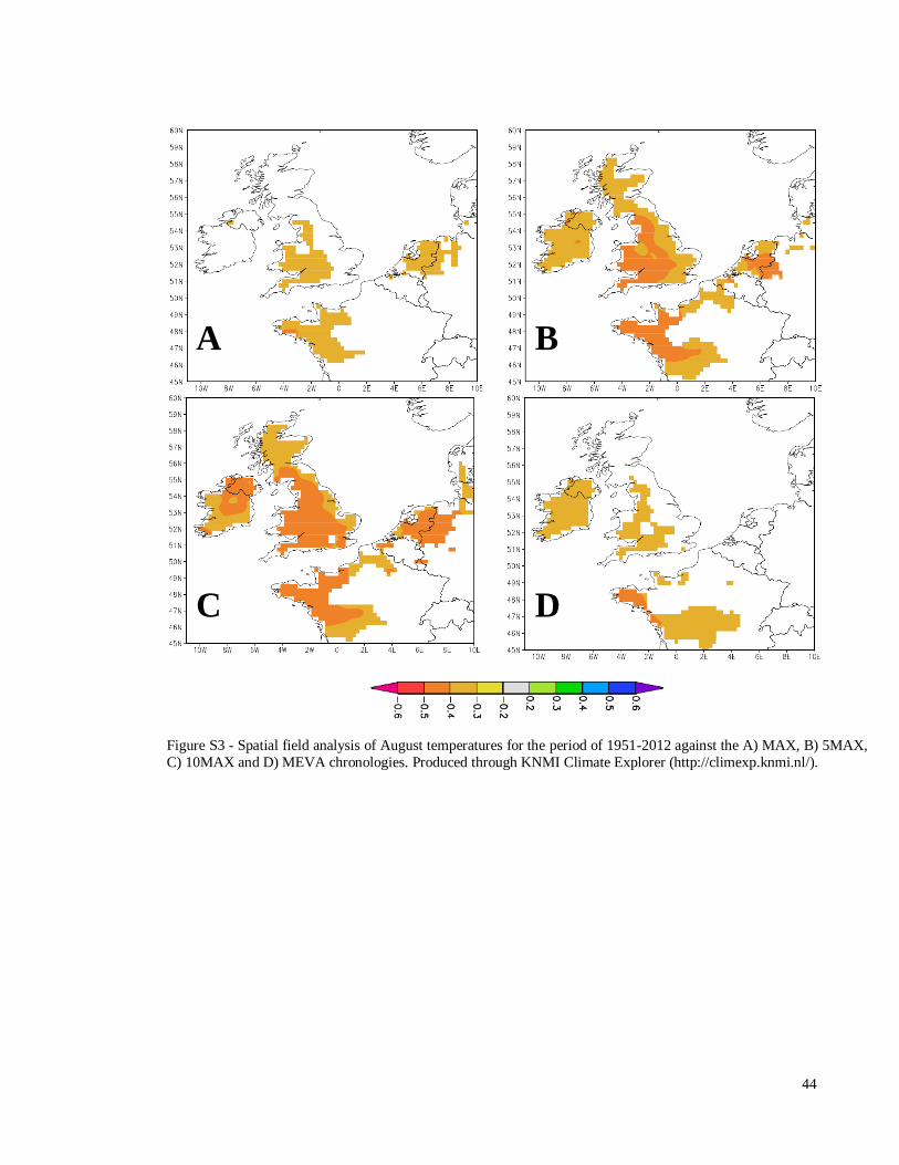
44

Figure S3 - Spatial field analysis of August temperatures for the period of 1951-2012 against the A) MAX, B) 5MAX,

C) 10MAX and D) MEVA chronologies. Produced through KNMI Climate Explorer (http://climexp.knmi.nl/).

A B

C D

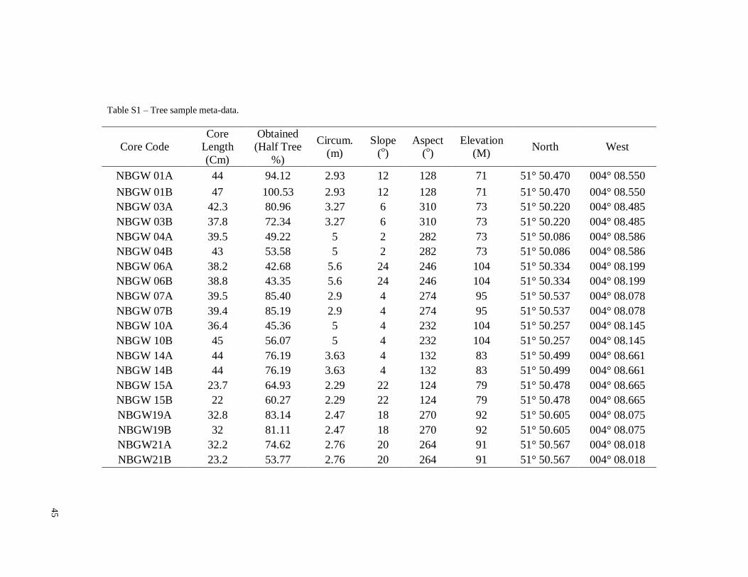
45

Table S1 – Tree sample meta-data.

Core Code

Core

Length

(Cm)

Obtained

(Half Tree

%)

Circum.

(m)

Slope

(o)

Aspect

(o)

Elevation

(M) North West

NBGW 01A 44 94.12 2.93 12 128 71 51° 50.470 004° 08.550

NBGW 01B 47 100.53 2.93 12 128 71 51° 50.470 004° 08.550

NBGW 03A 42.3 80.96 3.27 6 310 73 51° 50.220 004° 08.485

NBGW 03B 37.8 72.34 3.27 6 310 73 51° 50.220 004° 08.485

NBGW 04A 39.5 49.22 5 2 282 73 51° 50.086 004° 08.586

NBGW 04B 43 53.58 5 2 282 73 51° 50.086 004° 08.586

NBGW 06A 38.2 42.68 5.6 24 246 104 51° 50.334 004° 08.199

NBGW 06B 38.8 43.35 5.6 24 246 104 51° 50.334 004° 08.199

NBGW 07A 39.5 85.40 2.9 4 274 95 51° 50.537 004° 08.078

NBGW 07B 39.4 85.19 2.9 4 274 95 51° 50.537 004° 08.078

NBGW 10A 36.4 45.36 5 4 232 104 51° 50.257 004° 08.145

NBGW 10B 45 56.07 5 4 232 104 51° 50.257 004° 08.145

NBGW 14A 44 76.19 3.63 4 132 83 51° 50.499 004° 08.661

NBGW 14B 44 76.19 3.63 4 132 83 51° 50.499 004° 08.661

NBGW 15A 23.7 64.93 2.29 22 124 79 51° 50.478 004° 08.665

NBGW 15B 22 60.27 2.29 22 124 79 51° 50.478 004° 08.665

NBGW19A 32.8 83.14 2.47 18 270 92 51° 50.605 004° 08.075

NBGW19B 32 81.11 2.47 18 270 92 51° 50.605 004° 08.075

NBGW21A 32.2 74.62 2.76 20 264 91 51° 50.567 004° 08.018

NBGW21B 23.2 53.77 2.76 20 264 91 51° 50.567 004° 08.018

45

46

Table S2 -Filters used to identify and control abnormal

classifications

Filter Criteria

Area < 10,000 μm2

Area > 150,000 μm2

Length < 150 μm

Width < 50 μm

Width > 500 μm

Length / Width ratio < 0.05

Length / Width ratio > 1.9

47

Additional Data (separate files on CD)

Contained on the attached CD is a copy of the cross-dating statistics for the individual tree

cores (Database S1) and between the constructed master chronology and the master

chronology of Pilcher et al., (1984) (Database S2). Database S3 contains the master

chronology. Also contained is the raw (Database S4) and detrended vessel data (Database

S5).

48

Supplementary References

Alla, A. Q., & Camarero, J. J. (2012) “Contrasting responses of radial growth and wood

anatomy to climate in a Mediterranean ring-porous oak: implications for its future

persistence or why the variance matters more than the mean” European Journal of

Forest Research. 131. 1537 – 1550.

Baillie, M. G. L., & Pilcher, J. R. (1973) “A simple cross-dating program for tree-ring

research” Tree-Ring bulletin. 33. 7 – 14.

Fonti, P., & García-González, I. (2008) “Earlywood vessel size of oak as a potential proxy

for spring precipitation in mesic sites” Journal of Biogeography. 35. 2249 – 2257.

Fonti, P., Solomonoff, N., & García-González, I. (2007) “Earlywood vessels of Castanea

sativa recored temperature before their formation” New Phytologist. 173. 562 –

570.

Pilcher, J. R., Baillie, M. G. L., Schmidt, B., & Becker, B. (1984) “A 7,272 year tree-ring

chronology for western Europe” Nature. 312. 150 – 152.

Rinn, F. (2003) TSAP-Win-time series analysis and presentation dendrochronology and

related applications. Heidelberg: Frank Rinn.

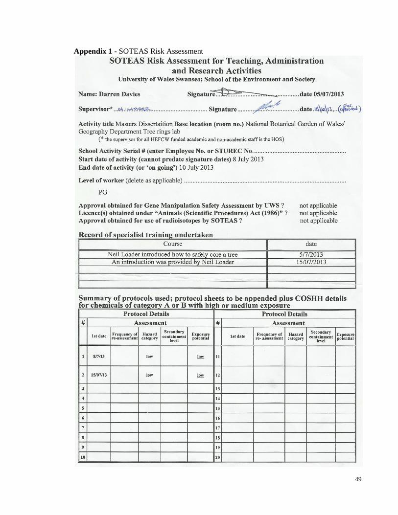
49

Appendix 1 - SOTEAS Risk Assessment

50

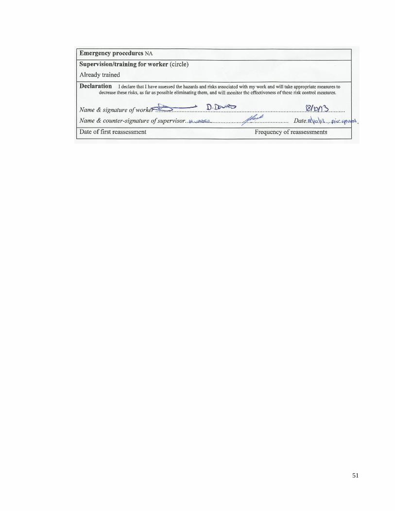
51

52

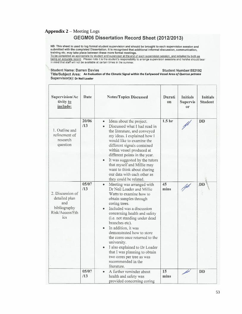
53

Appendix 2 – Meeting Logs

An Evaluation of the Climatic Signal within the Earlywood Vessel Area of Quercus petraea

Dr Neil Loader

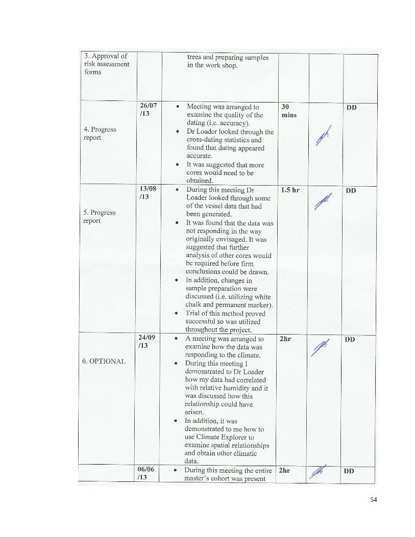
54

55