Embed Size (px)
Citation preview

Research in Mathematical Analysis – SomeConcrete Directions
Anthony Carbery
School of MathematicsUniversity of Edinburgh
Prospects in Mathematics, Durham, 9th January 2009
Anthony Carbery (U. of Edinburgh) 1 / 41

Outline
Outline
1 Overview
2 Fourier AnalysisA case study – the restriction of the Fourier Transform
3 PDEs
4 Geometric Measure Theory and Combinatorics in Fourier AnalysisA case study – Kakeya setsA case study – Anti-Kakeya sets
5 Number Theory
6 Conclusion
7 Further reading and other thoughts
Anthony Carbery (U. of Edinburgh) 2 / 41
Outline
Outline
1 Overview
2 Fourier AnalysisA case study – the restriction of the Fourier Transform
3 PDEs
4 Geometric Measure Theory and Combinatorics in Fourier AnalysisA case study – Kakeya setsA case study – Anti-Kakeya sets
5 Number Theory
6 Conclusion
7 Further reading and other thoughts
Anthony Carbery (U. of Edinburgh) 2 / 41

Outline
Outline
1 Overview
2 Fourier AnalysisA case study – the restriction of the Fourier Transform
3 PDEs
4 Geometric Measure Theory and Combinatorics in Fourier AnalysisA case study – Kakeya setsA case study – Anti-Kakeya sets
5 Number Theory
6 Conclusion
7 Further reading and other thoughts
Anthony Carbery (U. of Edinburgh) 2 / 41
Outline
Outline
1 Overview
2 Fourier AnalysisA case study – the restriction of the Fourier Transform
3 PDEs
4 Geometric Measure Theory and Combinatorics in Fourier AnalysisA case study – Kakeya setsA case study – Anti-Kakeya sets
5 Number Theory
6 Conclusion
7 Further reading and other thoughts
Anthony Carbery (U. of Edinburgh) 2 / 41

Outline
Outline
1 Overview
2 Fourier AnalysisA case study – the restriction of the Fourier Transform
3 PDEs
4 Geometric Measure Theory and Combinatorics in Fourier AnalysisA case study – Kakeya setsA case study – Anti-Kakeya sets
5 Number Theory
6 Conclusion
7 Further reading and other thoughts
Anthony Carbery (U. of Edinburgh) 2 / 41
Overview
Outline
1 Overview
2 Fourier AnalysisA case study – the restriction of the Fourier Transform
3 PDEs
4 Geometric Measure Theory and Combinatorics in Fourier AnalysisA case study – Kakeya setsA case study – Anti-Kakeya sets
5 Number Theory
6 Conclusion
7 Further reading and other thoughts
Anthony Carbery (U. of Edinburgh) 3 / 41

Overview
Undergraduate analysis
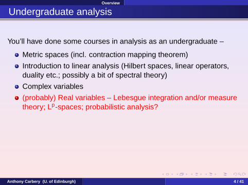
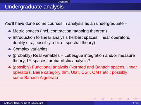
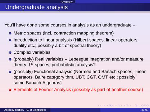
You’ll have done some courses in analysis as an undergraduate –
Metric spaces (incl. contraction mapping theorem)
Introduction to linear analysis (Hilbert spaces, linear operators,duality etc.; possibly a bit of spectral theory)
Complex variables
(probably) Real variables – Lebesgue integration and/or measuretheory; Lp-spaces; probabilistic analysis?
(possibly) Functional analysis (Normed and Banach spaces, linearoperators, Baire category thm, UBT, CGT, OMT etc.; possiblysome Banach Algebras)
Elements of Fourier Analysis (possibly as part of another course)
Anthony Carbery (U. of Edinburgh) 4 / 41

Overview
Undergraduate analysis
You’ll have done some courses in analysis as an undergraduate –
Metric spaces (incl. contraction mapping theorem)
Introduction to linear analysis (Hilbert spaces, linear operators,duality etc.; possibly a bit of spectral theory)
Complex variables
(probably) Real variables – Lebesgue integration and/or measuretheory; Lp-spaces; probabilistic analysis?
(possibly) Functional analysis (Normed and Banach spaces, linearoperators, Baire category thm, UBT, CGT, OMT etc.; possiblysome Banach Algebras)
Elements of Fourier Analysis (possibly as part of another course)
Anthony Carbery (U. of Edinburgh) 4 / 41

Overview
Undergraduate analysis
You’ll have done some courses in analysis as an undergraduate –
Metric spaces (incl. contraction mapping theorem)
Introduction to linear analysis (Hilbert spaces, linear operators,duality etc.; possibly a bit of spectral theory)
Complex variables
(probably) Real variables – Lebesgue integration and/or measuretheory; Lp-spaces; probabilistic analysis?
(possibly) Functional analysis (Normed and Banach spaces, linearoperators, Baire category thm, UBT, CGT, OMT etc.; possiblysome Banach Algebras)
Elements of Fourier Analysis (possibly as part of another course)
and you may or may not have covered some material in the area ofPDEs – e.g. Laplace’s equation, wave equation – most likely as part ofa “methods” course in applied maths.Anthony Carbery (U. of Edinburgh) 4 / 41
Overview
What’s next?
You are interested in doing a PhD in some area of analysis. How tochoose?
Anthony Carbery (U. of Edinburgh) 5 / 41
Overview
What’s next?
You are interested in doing a PhD in some area of analysis. How tochoose?
Some questions to ask yourself:
Anthony Carbery (U. of Edinburgh) 5 / 41

Overview
What’s next?
You are interested in doing a PhD in some area of analysis. How tochoose?
Some questions to ask yourself:
What style of analysis do I prefer – concrete or abstract, or a bit ofboth?
Anthony Carbery (U. of Edinburgh) 5 / 41

Overview
What’s next?
You are interested in doing a PhD in some area of analysis. How tochoose?
Some questions to ask yourself:
What style of analysis do I prefer – concrete or abstract, or a bit ofboth?
Which areas of modern analysis research suit my natural instincts?
Which areas of analysis are in a good state of health and are wellinterwoven in the mesh of greater mathematical activity?
To answer the last two you’ll need to know a bit about what are thecurrently active areas of research in analysis in the UK andinternationally.
DISCLAIMER: The remarks I’ll make on this issue are personal views.I’ll restrict myself to “Pure” Analysis – including PDE – and I’ll notdiscuss Applied Analysis at all.Anthony Carbery (U. of Edinburgh) 5 / 41

Overview
Different Styles of Mathematical Analysis
“Abstract” directions – areas in which the objects of analysis suchas Banach spaces, Hilbert spaces and classes of operators actingon them are studied in their own right and for their own sake.Typical starting point: “Let X be a Banach space.....”; the aim is tounderstand the internal structure of such objects. Some areas ofcurrent activity : C∗-algebras, operator algebras, operator spaces;Banach algebras. (The operator algebras group of areas hasgood connections with Mathematical Physics.)
“Mixed” directions – concrete situations where abstract methodsare prominent; abstract settings where the analysis is modelled ona previously understood concrete situation – e.g. ergodic theory(shift operators) & dynamical systems; operator theory; “local”theory of Banach spaces – the study of Rn as a Banach spacewith particular attention to dependence on n; probabalisticmethods.
Anthony Carbery (U. of Edinburgh) 6 / 41
Overview
Different Styles, cont’d
“Concrete” directions: e.g. Real Variables: geometric measuretheory, Fourier analysis, PDE; Complex analysis.
Anthony Carbery (U. of Edinburgh) 7 / 41

Overview
Different Styles, cont’d
“Concrete” directions: e.g. Real Variables: geometric measuretheory, Fourier analysis, PDE; Complex analysis.
This “classification” into abstract, concrete and mixed is very roughand ready and there are no firm boundaries.
Anthony Carbery (U. of Edinburgh) 7 / 41

Overview
Different Styles, cont’d
“Concrete” directions: e.g. Real Variables: geometric measuretheory, Fourier analysis, PDE; Complex analysis.
This “classification” into abstract, concrete and mixed is very roughand ready and there are no firm boundaries.
For the rest of the talk I’ll concentrate on the Real Variables themewithin “concrete” directions, beginning with some discussion of someof the ideas currently important in Fourier Analysis, and then we’ll seehow they link in with other areas.
Anthony Carbery (U. of Edinburgh) 7 / 41
Fourier Analysis
Outline
1 Overview
2 Fourier AnalysisA case study – the restriction of the Fourier Transform
3 PDEs
4 Geometric Measure Theory and Combinatorics in Fourier AnalysisA case study – Kakeya setsA case study – Anti-Kakeya sets
5 Number Theory
6 Conclusion
7 Further reading and other thoughts
Anthony Carbery (U. of Edinburgh) 8 / 41

Fourier Analysis
Fourier Analysis and its relations
We’ll look at a few examples of research topics in Fourier Analysis thatthe Edinburgh group has recently been involved in, and I’ll attempt toshow how these relate to other areas of analysis and mathematicsmore widely such as
Geometric measure theory
PDEs
Combinatorics
Number theory
Geometry (especially affine differential geometry)
Anthony Carbery (U. of Edinburgh) 9 / 41

Fourier Analysis
Fourier Analysis and its relations
We’ll look at a few examples of research topics in Fourier Analysis thatthe Edinburgh group has recently been involved in, and I’ll attempt toshow how these relate to other areas of analysis and mathematicsmore widely such as
Geometric measure theory
PDEs
Combinatorics
Number theory
Geometry (especially affine differential geometry)
The theme throughout is the interplay between specific operators andgeometrical considerations, sometimes based on symmetry, and howthis interplay is measured using specific spaces adapted to thegeometry at hand. Functional analysis and measure theory provide thelanguage for this discussion.
Anthony Carbery (U. of Edinburgh) 9 / 41

Fourier Analysis
Fourier Analysis – basics
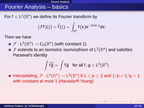
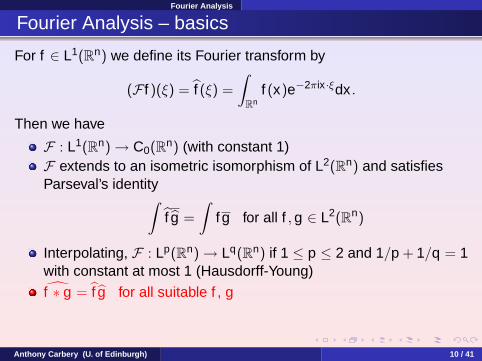
For f ∈ L1(Rn) we define its Fourier transform by
(F f )(ξ) = f (ξ) =
∫Rn
f (x)e−2πix ·ξdx .
Then we have
F : L1(Rn) → C0(Rn) (with constant 1)
F extends to an isometric isomorphism of L2(Rn) and satisfiesParseval’s identity∫
f g =
∫f g for all f , g ∈ L2(Rn)
Interpolating, F : Lp(Rn) → Lq(Rn) if 1 ≤ p ≤ 2 and 1/p + 1/q = 1with constant at most 1 (Hausdorff-Young)f ∗ g = f g for all suitable f , g
∂f/∂xj(ξ) = 2πiξj f (ξ) – smoothness of f implies decay of itsFourier transform
Anthony Carbery (U. of Edinburgh) 10 / 41

Fourier Analysis
Fourier Analysis – basics
For f ∈ L1(Rn) we define its Fourier transform by
(F f )(ξ) = f (ξ) =
∫Rn
f (x)e−2πix ·ξdx .
Then we have
F : L1(Rn) → C0(Rn) (with constant 1)F extends to an isometric isomorphism of L2(Rn) and satisfiesParseval’s identity∫
f g =
∫f g for all f , g ∈ L2(Rn)
Interpolating, F : Lp(Rn) → Lq(Rn) if 1 ≤ p ≤ 2 and 1/p + 1/q = 1with constant at most 1 (Hausdorff-Young)f ∗ g = f g for all suitable f , g
∂f/∂xj(ξ) = 2πiξj f (ξ) – smoothness of f implies decay of itsFourier transform
Anthony Carbery (U. of Edinburgh) 10 / 41
Fourier Analysis
Fourier Analysis – basics
For f ∈ L1(Rn) we define its Fourier transform by
(F f )(ξ) = f (ξ) =
∫Rn
f (x)e−2πix ·ξdx .
Then we have
F : L1(Rn) → C0(Rn) (with constant 1)F extends to an isometric isomorphism of L2(Rn) and satisfiesParseval’s identity∫
f g =
∫f g for all f , g ∈ L2(Rn)
Interpolating, F : Lp(Rn) → Lq(Rn) if 1 ≤ p ≤ 2 and 1/p + 1/q = 1with constant at most 1 (Hausdorff-Young)
f ∗ g = f g for all suitable f , g
∂f/∂xj(ξ) = 2πiξj f (ξ) – smoothness of f implies decay of itsFourier transform
Anthony Carbery (U. of Edinburgh) 10 / 41
Fourier Analysis
Fourier Analysis – basics
For f ∈ L1(Rn) we define its Fourier transform by
(F f )(ξ) = f (ξ) =
∫Rn
f (x)e−2πix ·ξdx .
Then we have
F : L1(Rn) → C0(Rn) (with constant 1)F extends to an isometric isomorphism of L2(Rn) and satisfiesParseval’s identity∫
f g =
∫f g for all f , g ∈ L2(Rn)
Interpolating, F : Lp(Rn) → Lq(Rn) if 1 ≤ p ≤ 2 and 1/p + 1/q = 1with constant at most 1 (Hausdorff-Young)f ∗ g = f g for all suitable f , g
∂f/∂xj(ξ) = 2πiξj f (ξ) – smoothness of f implies decay of itsFourier transform
Anthony Carbery (U. of Edinburgh) 10 / 41
Fourier Analysis A case study – the restriction of the Fourier Transform
Outline
1 Overview
2 Fourier AnalysisA case study – the restriction of the Fourier Transform
3 PDEs
4 Geometric Measure Theory and Combinatorics in Fourier AnalysisA case study – Kakeya setsA case study – Anti-Kakeya sets
5 Number Theory
6 Conclusion
7 Further reading and other thoughts
Anthony Carbery (U. of Edinburgh) 11 / 41

Fourier Analysis A case study – the restriction of the Fourier Transform
The restriction paradox
In particular, if f ∈ Lp with p a little bit larger than 1, all we can expect(via the Hausdorff-Young result) is for its Fourier transform to lie in Lq
where 1/p + 1/q = 1, and thus f is defined in principle only almosteverywhere on Rn, not genuinely pointwise.
Anthony Carbery (U. of Edinburgh) 12 / 41

Fourier Analysis A case study – the restriction of the Fourier Transform
The restriction paradox
In particular, if f ∈ Lp with p a little bit larger than 1, all we can expect(via the Hausdorff-Young result) is for its Fourier transform to lie in Lq
where 1/p + 1/q = 1, and thus f is defined in principle only almosteverywhere on Rn, not genuinely pointwise.
For a general function g ∈ Lq(Rn) we can alter it arbitrarily on a set ofmeasure zero without changing it as a member of Lq, and so the ideaof discussing g restricted to a set of measure zero makes no sense atall.
Nevertheless we are about to see that it makes perfectly good senseto talk about f restricted to a sphere.
Anthony Carbery (U. of Edinburgh) 12 / 41

Fourier Analysis A case study – the restriction of the Fourier Transform
Proof of restriction
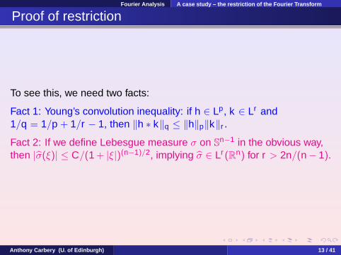
To see this, we need two facts:
Anthony Carbery (U. of Edinburgh) 13 / 41

Fourier Analysis A case study – the restriction of the Fourier Transform
Proof of restriction
To see this, we need two facts:
Fact 1: Young’s convolution inequality: if h ∈ Lp, k ∈ Lr and1/q = 1/p + 1/r − 1, then ‖h ∗ k‖q ≤ ‖h‖p‖k‖r .
Anthony Carbery (U. of Edinburgh) 13 / 41
Fourier Analysis A case study – the restriction of the Fourier Transform
Proof of restriction
To see this, we need two facts:
Fact 1: Young’s convolution inequality: if h ∈ Lp, k ∈ Lr and1/q = 1/p + 1/r − 1, then ‖h ∗ k‖q ≤ ‖h‖p‖k‖r .
Fact 2: If we define Lebesgue measure σ on Sn−1 in the obvious way,then |σ(ξ)| ≤ C/(1 + |ξ|)(n−1)/2, implying σ ∈ Lr (Rn) for r > 2n/(n− 1).
Anthony Carbery (U. of Edinburgh) 13 / 41

Fourier Analysis A case study – the restriction of the Fourier Transform
Proof of restriction
To see this, we need two facts:
Fact 1: Young’s convolution inequality: if h ∈ Lp, k ∈ Lr and1/q = 1/p + 1/r − 1, then ‖h ∗ k‖q ≤ ‖h‖p‖k‖r .
Fact 2: If we define Lebesgue measure σ on Sn−1 in the obvious way,then |σ(ξ)| ≤ C/(1 + |ξ|)(n−1)/2, implying σ ∈ Lr (Rn) for r > 2n/(n− 1).
Then we simply calculate:
∫Sn−1
|f (x)|2dσ(x) =
∫f f dσ
=
∫f f ∗ σ∨ ≤ ‖f‖p‖f ∗ σ∨‖q ≤ C‖f‖2
p
if p and r are related by 1/p + 1/q = 1, 1/q = 1/p + 1/r − 1 andr > 2n/(n − 1). Unravelling, this boils down to 1 ≤ p < 4n/(3n + 1),and so for p in this range, f exists as a member of L2(Sn−1).Anthony Carbery (U. of Edinburgh) 13 / 41

Fourier Analysis A case study – the restriction of the Fourier Transform
Features of argument
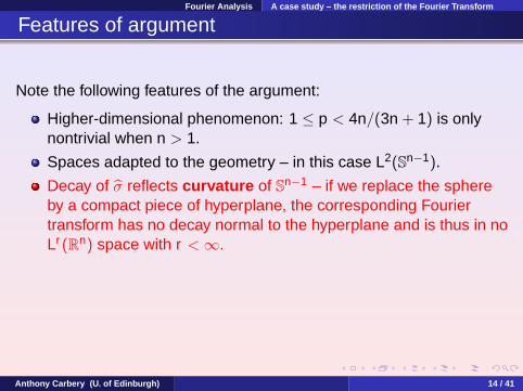
Note the following features of the argument:
Higher-dimensional phenomenon: 1 ≤ p < 4n/(3n + 1) is onlynontrivial when n > 1.
Spaces adapted to the geometry – in this case L2(Sn−1).
Decay of σ reflects curvature of Sn−1 – if we replace the sphereby a compact piece of hyperplane, the corresponding Fouriertransform has no decay normal to the hyperplane and is thus in noLr (Rn) space with r < ∞.
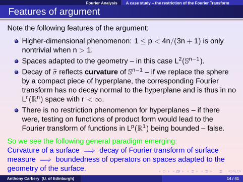
There is no restriction phenomenon for hyperplanes – if therewere, testing on functions of product form would lead to theFourier transform of functions in Lp(R1) being bounded – false.
Anthony Carbery (U. of Edinburgh) 14 / 41

Fourier Analysis A case study – the restriction of the Fourier Transform
Features of argument
Note the following features of the argument:
Higher-dimensional phenomenon: 1 ≤ p < 4n/(3n + 1) is onlynontrivial when n > 1.
Spaces adapted to the geometry – in this case L2(Sn−1).
Decay of σ reflects curvature of Sn−1 – if we replace the sphereby a compact piece of hyperplane, the corresponding Fouriertransform has no decay normal to the hyperplane and is thus in noLr (Rn) space with r < ∞.
There is no restriction phenomenon for hyperplanes – if therewere, testing on functions of product form would lead to theFourier transform of functions in Lp(R1) being bounded – false.
Anthony Carbery (U. of Edinburgh) 14 / 41
Fourier Analysis A case study – the restriction of the Fourier Transform
Features of argument
Note the following features of the argument:
Higher-dimensional phenomenon: 1 ≤ p < 4n/(3n + 1) is onlynontrivial when n > 1.
Spaces adapted to the geometry – in this case L2(Sn−1).
Decay of σ reflects curvature of Sn−1 – if we replace the sphereby a compact piece of hyperplane, the corresponding Fouriertransform has no decay normal to the hyperplane and is thus in noLr (Rn) space with r < ∞.
There is no restriction phenomenon for hyperplanes – if therewere, testing on functions of product form would lead to theFourier transform of functions in Lp(R1) being bounded – false.
So we see the following general paradigm emerging:Curvature of a surface =⇒ decay of Fourier transform of surfacemeasure =⇒ boundedness of operators on spaces adapted to thegeometry of the surface.Anthony Carbery (U. of Edinburgh) 14 / 41

Fourier Analysis A case study – the restriction of the Fourier Transform
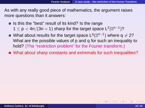
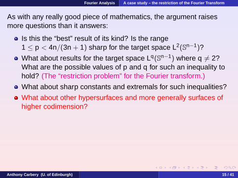
As with any really good piece of mathematics, the argument raisesmore questions than it answers:
Is this the “best” result of its kind? Is the range1 ≤ p < 4n/(3n + 1) sharp for the target space L2(Sn−1)?
What about results for the target space Lq(Sn−1) where q 6= 2?What are the possible values of p and q for such an inequality tohold? (The “restriction problem” for the Fourier transform.)
What about sharp constants and extremals for such inequalities?
What about other hypersurfaces and more generally surfaces ofhigher codimension?
“Best” rates of decay for Fourier transforms of measuressupported on curved submanifolds of Rn?
Given a curved submanifold, in what precise way does its“curvature” affect matters? Is there an “optimal” choice ofmeasure to put on it to make things work well?
Anthony Carbery (U. of Edinburgh) 15 / 41

Fourier Analysis A case study – the restriction of the Fourier Transform
As with any really good piece of mathematics, the argument raisesmore questions than it answers:
Is this the “best” result of its kind? Is the range1 ≤ p < 4n/(3n + 1) sharp for the target space L2(Sn−1)?
What about results for the target space Lq(Sn−1) where q 6= 2?What are the possible values of p and q for such an inequality tohold? (The “restriction problem” for the Fourier transform.)
What about sharp constants and extremals for such inequalities?
What about other hypersurfaces and more generally surfaces ofhigher codimension?
“Best” rates of decay for Fourier transforms of measuressupported on curved submanifolds of Rn?
Given a curved submanifold, in what precise way does its“curvature” affect matters? Is there an “optimal” choice ofmeasure to put on it to make things work well?
Anthony Carbery (U. of Edinburgh) 15 / 41

Fourier Analysis A case study – the restriction of the Fourier Transform
And as with any really good piece of mathematics, it turns out to havelinks and implications well beyond its initial confines into broadermathematical analysis and beyond.....
Anthony Carbery (U. of Edinburgh) 16 / 41

Fourier Analysis A case study – the restriction of the Fourier Transform
And as with any really good piece of mathematics, it turns out to havelinks and implications well beyond its initial confines into broadermathematical analysis and beyond.....
Example (Jim Wright and co-authors) A new affine isoperimetricinequality for the class of polynomial curves in Rn.
Let Γ : I → Rn be a curve all of whose components are polynomial.The total affine curvature of Γ is the quantity
A(Γ) =
∫Idet(Γ′(t), Γ′′(t), . . . , Γ(n)(t)
)2/n(n+1)dt .
Then there is a constant C depending only on the degree of Γ and thedimension n so that
A(Γ) ≤ C vol (cvx{Γ(t) : t ∈ I})2/n(n+1) .
Again, more questions arise: What about non-polynomial curves?What about extremals and best constants? What abouthigher-dimensional surfaces?Anthony Carbery (U. of Edinburgh) 16 / 41

PDEs
Outline
1 Overview
2 Fourier AnalysisA case study – the restriction of the Fourier Transform
3 PDEs
4 Geometric Measure Theory and Combinatorics in Fourier AnalysisA case study – Kakeya setsA case study – Anti-Kakeya sets
5 Number Theory
6 Conclusion
7 Further reading and other thoughts
Anthony Carbery (U. of Edinburgh) 17 / 41
PDEs
PDEs in Pure Maths
A lot of mathematics undergraduates don’t realise that a great deal ofPDE research activity is much more “pure” mathematical than applied.This sort of rigorous PDE research falls square under the heading of“concrete directions in analysis”.
Anthony Carbery (U. of Edinburgh) 18 / 41

PDEs
PDEs in Pure Maths
A lot of mathematics undergraduates don’t realise that a great deal ofPDE research activity is much more “pure” mathematical than applied.This sort of rigorous PDE research falls square under the heading of“concrete directions in analysis”.
It doesn’t much matter whether you’ve had a throrough course inPDE methods as an undergraduate, what is important is a goodbackground in the sort of analysis we’ve already been talking about –metric spaces, linear analysis, real variables, Fourier Analysis – and adesire to work further in areas which use this sort of mathematics.
Anthony Carbery (U. of Edinburgh) 18 / 41
PDEs
PDEs in Pure Maths
A lot of mathematics undergraduates don’t realise that a great deal ofPDE research activity is much more “pure” mathematical than applied.This sort of rigorous PDE research falls square under the heading of“concrete directions in analysis”.
It doesn’t much matter whether you’ve had a throrough course inPDE methods as an undergraduate, what is important is a goodbackground in the sort of analysis we’ve already been talking about –metric spaces, linear analysis, real variables, Fourier Analysis – and adesire to work further in areas which use this sort of mathematics.
Any odd “methodsy” bits can be easily picked up as you go along.
Anthony Carbery (U. of Edinburgh) 18 / 41
PDEs
PDEs in Pure Maths, cont’d
Typically, the issues are the theoretical issues of existence anduniqueness (and perhaps well-posedness i.e. good sensitivity to smallchanges in initial data) for classes of linear and nonlinear PDE (whichdo admittedly arise in real life).
Anthony Carbery (U. of Edinburgh) 19 / 41
PDEs
PDEs in Pure Maths, cont’d
Typically, the issues are the theoretical issues of existence anduniqueness (and perhaps well-posedness i.e. good sensitivity to smallchanges in initial data) for classes of linear and nonlinear PDE (whichdo admittedly arise in real life).
The main questions which arise become, often, questions ofboundedness (or continuity) of certain specific linear or nonlinearoperators on certain specific spaces adapted to the problems at hand.
Anthony Carbery (U. of Edinburgh) 19 / 41

PDEs
PDEs in Pure Maths, cont’d
Typically, the issues are the theoretical issues of existence anduniqueness (and perhaps well-posedness i.e. good sensitivity to smallchanges in initial data) for classes of linear and nonlinear PDE (whichdo admittedly arise in real life).
The main questions which arise become, often, questions ofboundedness (or continuity) of certain specific linear or nonlinearoperators on certain specific spaces adapted to the problems at hand.
There is a great deal of investment (both money and people) in thisarea curently in the UK – average academic job prospects for a goodPhD graduate in theoretical PDE are somewhat better than those inmaths more generally.
Anthony Carbery (U. of Edinburgh) 19 / 41

PDEs
Laplace’s equation
Example 1. Laplace’s equation on “rough” domains. Let G ⊆ Rn
be a domain whose boundary is not presumed to be smooth. So it canhave edges, corners, even possibly a fractal-like structure. For manyreasons it’s important to understand the equation
4u = 0 on G
with boundary data f ∈ Lp(∂G) for some 1 < p < ∞.
Anthony Carbery (U. of Edinburgh) 20 / 41

PDEs
Laplace’s equation
Example 1. Laplace’s equation on “rough” domains. Let G ⊆ Rn
be a domain whose boundary is not presumed to be smooth. So it canhave edges, corners, even possibly a fractal-like structure. For manyreasons it’s important to understand the equation
4u = 0 on G
with boundary data f ∈ Lp(∂G) for some 1 < p < ∞.
When G is the unit ball or the upper-half-space [with the extra conditionthat u vanish at ∞ thrown in], this is classical Fourier analysis, and theunique solution is obtained by integrating f against the Poisson kernel.
Even in this case, it is not immediately clear in what sense the solutionu(x) converges to the boundary data f as x moves towards theboundary as f is only defined almost everywhere. To handle this weneed “maximal” functions.
Anthony Carbery (U. of Edinburgh) 20 / 41
PDEs
Laplace’s equation
Example 1. Laplace’s equation on “rough” domains. Let G ⊆ Rn
be a domain whose boundary is not presumed to be smooth. So it canhave edges, corners, even possibly a fractal-like structure. For manyreasons it’s important to understand the equation
4u = 0 on G
with boundary data f ∈ Lp(∂G) for some 1 < p < ∞.
In the general case there are many issues: what is the measure to beused on ∂G? (There are at least two possible natural candidiates).Can we “construct” a Poisson kernel and/or a Green’s function? Inwhat sense does the resulting Poisson integral actually solve theproblem? Are solutions unique? Do we get almost-everywhereconvergence of the solution back to the boundary data?
Martin Dindos and his group work on questions like these.....
Anthony Carbery (U. of Edinburgh) 20 / 41

PDEs
NLS
Example 2. Nonlinear Schr odinger equation.
The linear Schrodinger equation for (x , t) ∈ Rn × R is
4u = i∂u/∂t
with initial data u(x , 0) = f (x).
Anthony Carbery (U. of Edinburgh) 21 / 41

PDEs
NLS
Example 2. Nonlinear Schr odinger equation.
The linear Schrodinger equation for (x , t) ∈ Rn × R is
4u = i∂u/∂t
with initial data u(x , 0) = f (x).
We can (in principle) write down the solution to this equation:
u(x , t) = f ∗ Kt(x) where Kt(x) = t−n/2e2πi|x |2/t .
The nonlinear Schrodinger equation introduces a nonlinear functionh(u) (which we may take to be essentially a monomial) and asks tosolve
4u − i∂u/∂t = h(u), with u(x , 0) = f .
Anthony Carbery (U. of Edinburgh) 21 / 41

PDEs
NLS, cont’d
Typically, the analysis of NLS falls into two parts:
Finding a complete metric spaces of functions and a map betweenthem so that the solution is a fixed point of this map – nonlinearanalysis
Showing that the map is actually a contraction – linear analysis
Anthony Carbery (U. of Edinburgh) 22 / 41

PDEs
NLS, cont’d
Typically, the analysis of NLS falls into two parts:
Finding a complete metric spaces of functions and a map betweenthem so that the solution is a fixed point of this map – nonlinearanalysis
Showing that the map is actually a contraction – linear analysis
The latter is carried out by understanding the solution operatorf 7→ f ∗ Kt(x) to the linear problem very well. This is a matter of FourierAnalysis.
Anthony Carbery (U. of Edinburgh) 22 / 41
PDEs
NLS, cont’d
Typically, the analysis of NLS falls into two parts:
Finding a complete metric spaces of functions and a map betweenthem so that the solution is a fixed point of this map – nonlinearanalysis
Showing that the map is actually a contraction – linear analysis
The latter is carried out by understanding the solution operatorf 7→ f ∗ Kt(x) to the linear problem very well. This is a matter of FourierAnalysis.
Questions like this are investigated by Nikolaos Bournaveas and PieterBlue.
Anthony Carbery (U. of Edinburgh) 22 / 41

PDEs
NLS and restriction
Amazing link: the Schrodinger solution operator
f 7→ u(x , t) = f ∗ Kt(x) := St f (x)
is PRECISELY the adjoint of the restriction operator for the paraboloidapplied to f .
Anthony Carbery (U. of Edinburgh) 23 / 41

PDEs
NLS and restriction
Amazing link: the Schrodinger solution operator
f 7→ u(x , t) = f ∗ Kt(x) := St f (x)
is PRECISELY the adjoint of the restriction operator for the paraboloidapplied to f .
That is, if we define R to be the restriction map taking functions onRn+1 to functions on Rn given by
(Rg)(x) = g(x , |x |2/2)
thenSt f (x) = R∗ f (x , t).
This means that all of the theory developed for the (Fourier Analytic)restriction phenomenon is immediately applicable to problems innonlinear PDE! In the PDE literature these are called “Strichartzestimates”.Anthony Carbery (U. of Edinburgh) 23 / 41
GMT & Combinatorics
Outline
1 Overview
2 Fourier AnalysisA case study – the restriction of the Fourier Transform
3 PDEs
4 Geometric Measure Theory and Combinatorics in Fourier AnalysisA case study – Kakeya setsA case study – Anti-Kakeya sets
5 Number Theory
6 Conclusion
7 Further reading and other thoughts
Anthony Carbery (U. of Edinburgh) 24 / 41
GMT & Combinatorics A case study – Kakeya sets
Outline
1 Overview
2 Fourier AnalysisA case study – the restriction of the Fourier Transform
3 PDEs
4 Geometric Measure Theory and Combinatorics in Fourier AnalysisA case study – Kakeya setsA case study – Anti-Kakeya sets
5 Number Theory
6 Conclusion
7 Further reading and other thoughts
Anthony Carbery (U. of Edinburgh) 25 / 41
GMT & Combinatorics A case study – Kakeya sets
Kakeya sets
A Kakeya or Besicovitch set is a set E ⊆ Rn which contains at leastone unit line segment `ω in each direction ω ∈ Sn−1.
Anthony Carbery (U. of Edinburgh) 26 / 41

GMT & Combinatorics A case study – Kakeya sets
Kakeya sets
A Kakeya or Besicovitch set is a set E ⊆ Rn which contains at leastone unit line segment `ω in each direction ω ∈ Sn−1. So a Kakeya setis “large”, and it makes sense to ask how large it must be in terms of its(possibly fractional) dimension.
Anthony Carbery (U. of Edinburgh) 26 / 41
GMT & Combinatorics A case study – Kakeya sets
Kakeya sets
A Kakeya or Besicovitch set is a set E ⊆ Rn which contains at leastone unit line segment `ω in each direction ω ∈ Sn−1. So a Kakeya setis “large”, and it makes sense to ask how large it must be in terms of its(possibly fractional) dimension.
Conjecture: Any Kakeya set must have dimension n. (This is onlyknown to be true when n = 2.)
Anthony Carbery (U. of Edinburgh) 26 / 41

GMT & Combinatorics A case study – Kakeya sets
Kakeya sets
A Kakeya or Besicovitch set is a set E ⊆ Rn which contains at leastone unit line segment `ω in each direction ω ∈ Sn−1. So a Kakeya setis “large”, and it makes sense to ask how large it must be in terms of its(possibly fractional) dimension.
Conjecture: Any Kakeya set must have dimension n. (This is onlyknown to be true when n = 2.)
What does this have to do with Fourier Analysis?
It turns out that if we could completely solve the restriction problem forthe Fourier transform, the conjecture would follow by the followingroute:
Anthony Carbery (U. of Edinburgh) 26 / 41

GMT & Combinatorics A case study – Kakeya sets
Restriction implies Kakeya
Suppose R : L2n/(n+1)(Rn) → L2n/(n+1)(Sn−1) boundedly. (A slightlie here.) By duality, R∗ : L2n/(n−1)(Sn−1) → L2n/(n−1)(Rn).
Apply this to a well-chosen family of examples, and then averageover the family, yielding∫
B
(∑T∈T
αT χT
)n/(n−1)
≤ Cn(log N)N−(n−1)∑
T
αn/(n−1)T
whenever T is a family of rectangles of sides 1/N × 1/N × · · · × 1,for a large parameter N, with one in each of the essentially Nn−1
different directions.This implies
| ∪T∈T T |∑T∈T |T |
≥ Cn
(log N)n−1
which is a quantitiative version of the claim on the dimension of aKakeya set.
Anthony Carbery (U. of Edinburgh) 27 / 41

GMT & Combinatorics A case study – Kakeya sets
Restriction implies Kakeya
Suppose R : L2n/(n+1)(Rn) → L2n/(n+1)(Sn−1) boundedly. (A slightlie here.) By duality, R∗ : L2n/(n−1)(Sn−1) → L2n/(n−1)(Rn).Apply this to a well-chosen family of examples, and then averageover the family, yielding∫
B
(∑T∈T
αT χT
)n/(n−1)
≤ Cn(log N)N−(n−1)∑
T
αn/(n−1)T
whenever T is a family of rectangles of sides 1/N × 1/N × · · · × 1,for a large parameter N, with one in each of the essentially Nn−1
different directions.
This implies| ∪T∈T T |∑
T∈T |T |≥ Cn
(log N)n−1
which is a quantitiative version of the claim on the dimension of aKakeya set.
Anthony Carbery (U. of Edinburgh) 27 / 41

GMT & Combinatorics A case study – Kakeya sets
Restriction implies Kakeya
Suppose R : L2n/(n+1)(Rn) → L2n/(n+1)(Sn−1) boundedly. (A slightlie here.) By duality, R∗ : L2n/(n−1)(Sn−1) → L2n/(n−1)(Rn).Apply this to a well-chosen family of examples, and then averageover the family, yielding∫
B
(∑T∈T
αT χT
)n/(n−1)
≤ Cn(log N)N−(n−1)∑
T
αn/(n−1)T
whenever T is a family of rectangles of sides 1/N × 1/N × · · · × 1,for a large parameter N, with one in each of the essentially Nn−1
different directions.This implies
| ∪T∈T T |∑T∈T |T |
≥ Cn
(log N)n−1
which is a quantitiative version of the claim on the dimension of aKakeya set.
Anthony Carbery (U. of Edinburgh) 27 / 41

GMT & Combinatorics A case study – Kakeya sets
n = 2 and maximal functions
The previous inequality∫B
(∑T∈T
αT χT
)n/(n−1)
≤ Cn(log N)N−(n−1)∑
T
αn/(n−1)T
has two noteworthy features:
When n = 2, the exponent n/(n − 1) is just 2, and one can simplymultiply out to prove it, using one’s knowledge of the area of theintersection of two rectangles, i.e. a parallelogram!
In general, the inequality has a dual form expressed in terms ofmaximal functions: let
MN f (x) = supx∈T
1|T |
∫T
f
where the sup is taken over the family of all 1/N × 1/N × · · · × 1rectangles T passing through x . Then it’s equivalent via duality to
‖MN f‖n ≤ Cn(log N)(n−1)/n‖f‖n.
Anthony Carbery (U. of Edinburgh) 28 / 41

GMT & Combinatorics A case study – Kakeya sets
n = 2 and maximal functions
The previous inequality∫B
(∑T∈T
αT χT
)n/(n−1)
≤ Cn(log N)N−(n−1)∑
T
αn/(n−1)T
has two noteworthy features:
When n = 2, the exponent n/(n − 1) is just 2, and one can simplymultiply out to prove it, using one’s knowledge of the area of theintersection of two rectangles, i.e. a parallelogram!In general, the inequality has a dual form expressed in terms ofmaximal functions: let
MN f (x) = supx∈T
1|T |
∫T
f
where the sup is taken over the family of all 1/N × 1/N × · · · × 1rectangles T passing through x . Then it’s equivalent via duality to
‖MN f‖n ≤ Cn(log N)(n−1)/n‖f‖n.
Anthony Carbery (U. of Edinburgh) 28 / 41

GMT & Combinatorics A case study – Kakeya sets
Higher dimensions?
When n ≥ 3 one cannot simply multiply out. Partial progress has beenmade by various authors. Recently, with Bennett and Tao, weconsidered a multilinear variant of the main inequality and proved it “upto end points” using a novel heat-flow method. The main “geometric”interpretation of our results is as follows:
Anthony Carbery (U. of Edinburgh) 29 / 41

GMT & Combinatorics A case study – Kakeya sets
Higher dimensions?
When n ≥ 3 one cannot simply multiply out. Partial progress has beenmade by various authors. Recently, with Bennett and Tao, weconsidered a multilinear variant of the main inequality and proved it “upto end points” using a novel heat-flow method. The main “geometric”interpretation of our results is as follows:
Consider a family L of M lines in Rn. Define a joint to be anintersection of n lines in L lying in no affine hyperplane. We say a jointis transverse if the parallepiped formed using unit vectors in thedirections of the lines has volume bounded below.
Anthony Carbery (U. of Edinburgh) 29 / 41

GMT & Combinatorics A case study – Kakeya sets
Higher dimensions?
When n ≥ 3 one cannot simply multiply out. Partial progress has beenmade by various authors. Recently, with Bennett and Tao, weconsidered a multilinear variant of the main inequality and proved it “upto end points” using a novel heat-flow method. The main “geometric”interpretation of our results is as follows:
Consider a family L of M lines in Rn. Define a joint to be anintersection of n lines in L lying in no affine hyperplane. We say a jointis transverse if the parallepiped formed using unit vectors in thedirections of the lines has volume bounded below. Then the numberof transverse joints is bounded by CnMn/(n−1)+.
Last month, Guth and Katz disposed of the word “transverse” and the“+”. They used totally unrelated methods – topology, algebraicgeometry, cohomology, commutative diagrams, building on work ofGromov. These have further implications for “pure” GeometricMeasure Theory which have yet to be explored.....
Anthony Carbery (U. of Edinburgh) 29 / 41

GMT & Combinatorics A case study – Anti-Kakeya sets
Outline
1 Overview
2 Fourier AnalysisA case study – the restriction of the Fourier Transform
3 PDEs
4 Geometric Measure Theory and Combinatorics in Fourier AnalysisA case study – Kakeya setsA case study – Anti-Kakeya sets
5 Number Theory
6 Conclusion
7 Further reading and other thoughts
Anthony Carbery (U. of Edinburgh) 30 / 41

GMT & Combinatorics A case study – Anti-Kakeya sets
Anti-Kakeya sets
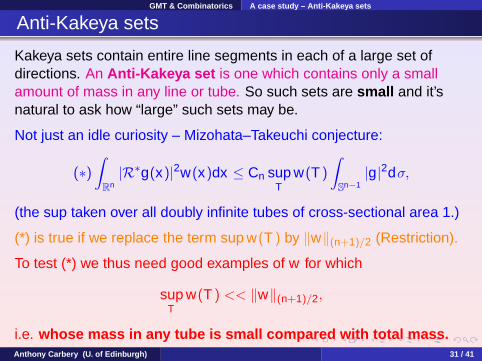
Kakeya sets contain entire line segments in each of a large set ofdirections. An Anti-Kakeya set is one which contains only a smallamount of mass in any line or tube. So such sets are small and it’snatural to ask how “large” such sets may be.
Anthony Carbery (U. of Edinburgh) 31 / 41

GMT & Combinatorics A case study – Anti-Kakeya sets
Anti-Kakeya sets
Kakeya sets contain entire line segments in each of a large set ofdirections. An Anti-Kakeya set is one which contains only a smallamount of mass in any line or tube. So such sets are small and it’snatural to ask how “large” such sets may be.
Not just an idle curiosity – Mizohata–Takeuchi conjecture:
(∗)∫
Rn|R∗g(x)|2w(x)dx ≤ Cn sup
Tw(T )
∫Sn−1
|g|2dσ,
(the sup taken over all doubly infinite tubes of cross-sectional area 1.)
(*) is true if we replace the term sup w(T ) by ‖w‖(n+1)/2 (Restriction).
Anthony Carbery (U. of Edinburgh) 31 / 41
GMT & Combinatorics A case study – Anti-Kakeya sets
Anti-Kakeya sets
Kakeya sets contain entire line segments in each of a large set ofdirections. An Anti-Kakeya set is one which contains only a smallamount of mass in any line or tube. So such sets are small and it’snatural to ask how “large” such sets may be.
Not just an idle curiosity – Mizohata–Takeuchi conjecture:
(∗)∫
Rn|R∗g(x)|2w(x)dx ≤ Cn sup
Tw(T )
∫Sn−1
|g|2dσ,
(the sup taken over all doubly infinite tubes of cross-sectional area 1.)
(*) is true if we replace the term sup w(T ) by ‖w‖(n+1)/2 (Restriction).
To test (*) we thus need good examples of w for which
supT
w(T ) << ‖w‖(n+1)/2,
i.e. whose mass in any tube is small compared with total mass.Anthony Carbery (U. of Edinburgh) 31 / 41
GMT & Combinatorics A case study – Anti-Kakeya sets
A Challenge
In this spirit, consider an N × N array of black and white unit squares.How many squares can be coloured black to that no strip of width 1meets more than two of them?
Anthony Carbery (U. of Edinburgh) 32 / 41

GMT & Combinatorics A case study – Anti-Kakeya sets
A Challenge
In this spirit, consider an N × N array of black and white unit squares.How many squares can be coloured black to that no strip of width 1meets more than two of them?
It’s not hard to see that one can colour at least cN1/2 squares black.(In fact, there’s a logarithmic improvement on this.)
But now ask that no strip meet more than 3 of them.
Exercise: Find an example of such with at least cN2/3 coloured black.
The true orders Nα in these and similar problems are unknown.
Anthony Carbery (U. of Edinburgh) 32 / 41
GMT & Combinatorics A case study – Anti-Kakeya sets
Tube-nullity
Closely related is tube-nullity. A set E ⊆ Rn is tube-null if it can becovered by a collection of tubes the sum of whose cross-sectionalareas is arbitrarily small.
Anthony Carbery (U. of Edinburgh) 33 / 41
GMT & Combinatorics A case study – Anti-Kakeya sets
Tube-nullity
Closely related is tube-nullity. A set E ⊆ Rn is tube-null if it can becovered by a collection of tubes the sum of whose cross-sectionalareas is arbitrarily small.
So this is another sort of “smallness” condition: tube-null sets arealways Lebesgue-null; any reasonable set of dimension at most n − 1is tube-null, but there do exist tube-null sets of full dimension n.
Anthony Carbery (U. of Edinburgh) 33 / 41

GMT & Combinatorics A case study – Anti-Kakeya sets
Tube-nullity
Closely related is tube-nullity. A set E ⊆ Rn is tube-null if it can becovered by a collection of tubes the sum of whose cross-sectionalareas is arbitrarily small.
So this is another sort of “smallness” condition: tube-null sets arealways Lebesgue-null; any reasonable set of dimension at most n − 1is tube-null, but there do exist tube-null sets of full dimension n.
This notion arises in Fourier Analysis when consideringhigher-dimensional analogues of Riemann’s localisation theorem(stating that convergence of a Fourier series at a given point is dictatedentirely by the values of the function near that point).
Anthony Carbery (U. of Edinburgh) 33 / 41
GMT & Combinatorics A case study – Anti-Kakeya sets
Tube-nullity
Closely related is tube-nullity. A set E ⊆ Rn is tube-null if it can becovered by a collection of tubes the sum of whose cross-sectionalareas is arbitrarily small.
So this is another sort of “smallness” condition: tube-null sets arealways Lebesgue-null; any reasonable set of dimension at most n − 1is tube-null, but there do exist tube-null sets of full dimension n.
Question 1. Do there exist non-tube-null sets of each dimensiongreater than n − 1?
Anthony Carbery (U. of Edinburgh) 33 / 41

GMT & Combinatorics A case study – Anti-Kakeya sets
Tube-nullity
Closely related is tube-nullity. A set E ⊆ Rn is tube-null if it can becovered by a collection of tubes the sum of whose cross-sectionalareas is arbitrarily small.
So this is another sort of “smallness” condition: tube-null sets arealways Lebesgue-null; any reasonable set of dimension at most n − 1is tube-null, but there do exist tube-null sets of full dimension n.
Question 1. Do there exist non-tube-null sets of each dimensiongreater than n − 1?
Question 2. Is the radial outer 2 quarters Cantor set based on [1,2]tube-null?
Question 3. Do there exist tube-null Kakeya sets? Is every Kakeya settube-null?
Anthony Carbery (U. of Edinburgh) 33 / 41

Number Theory
Outline
1 Overview
2 Fourier AnalysisA case study – the restriction of the Fourier Transform
3 PDEs
4 Geometric Measure Theory and Combinatorics in Fourier AnalysisA case study – Kakeya setsA case study – Anti-Kakeya sets
5 Number Theory
6 Conclusion
7 Further reading and other thoughts
Anthony Carbery (U. of Edinburgh) 34 / 41
Number Theory
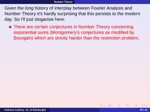
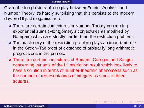
Given the long history of interplay between Fourier Analysis andNumber Theory it’s hardly surprising that this persists to the modernday. So I’ll just sloganise here:
There are certain conjectures in Number Theory concerningexponential sums (Montgomery’s conjectures as modified byBourgain) which are strictly harder than the restriction problem.
The machinery of the restriction problem plays an important rolein the Green–Tao proof of existence of arbitrarily long arithmeticprogressions in the primes.There are certain conjectures of Bonami, Garrigos and Seegerconcerning variants of the L2 restriction result which look likely tohave a solution in terms of number-theoretic phenomena such asthe number of representations of integers as sums of threesquares.Jim Wright is developing a programme of heuristics linking resultsfor sublevel sets, oscillatory integrals and averaging opertors inFourier Analysis to their number-theoretic counterparts.
Anthony Carbery (U. of Edinburgh) 35 / 41

Number Theory
Given the long history of interplay between Fourier Analysis andNumber Theory it’s hardly surprising that this persists to the modernday. So I’ll just sloganise here:
There are certain conjectures in Number Theory concerningexponential sums (Montgomery’s conjectures as modified byBourgain) which are strictly harder than the restriction problem.The machinery of the restriction problem plays an important rolein the Green–Tao proof of existence of arbitrarily long arithmeticprogressions in the primes.
There are certain conjectures of Bonami, Garrigos and Seegerconcerning variants of the L2 restriction result which look likely tohave a solution in terms of number-theoretic phenomena such asthe number of representations of integers as sums of threesquares.Jim Wright is developing a programme of heuristics linking resultsfor sublevel sets, oscillatory integrals and averaging opertors inFourier Analysis to their number-theoretic counterparts.
Anthony Carbery (U. of Edinburgh) 35 / 41
Number Theory
Given the long history of interplay between Fourier Analysis andNumber Theory it’s hardly surprising that this persists to the modernday. So I’ll just sloganise here:
There are certain conjectures in Number Theory concerningexponential sums (Montgomery’s conjectures as modified byBourgain) which are strictly harder than the restriction problem.The machinery of the restriction problem plays an important rolein the Green–Tao proof of existence of arbitrarily long arithmeticprogressions in the primes.There are certain conjectures of Bonami, Garrigos and Seegerconcerning variants of the L2 restriction result which look likely tohave a solution in terms of number-theoretic phenomena such asthe number of representations of integers as sums of threesquares.
Jim Wright is developing a programme of heuristics linking resultsfor sublevel sets, oscillatory integrals and averaging opertors inFourier Analysis to their number-theoretic counterparts.
Anthony Carbery (U. of Edinburgh) 35 / 41

Number Theory
Given the long history of interplay between Fourier Analysis andNumber Theory it’s hardly surprising that this persists to the modernday. So I’ll just sloganise here:
There are certain conjectures in Number Theory concerningexponential sums (Montgomery’s conjectures as modified byBourgain) which are strictly harder than the restriction problem.The machinery of the restriction problem plays an important rolein the Green–Tao proof of existence of arbitrarily long arithmeticprogressions in the primes.There are certain conjectures of Bonami, Garrigos and Seegerconcerning variants of the L2 restriction result which look likely tohave a solution in terms of number-theoretic phenomena such asthe number of representations of integers as sums of threesquares.Jim Wright is developing a programme of heuristics linking resultsfor sublevel sets, oscillatory integrals and averaging opertors inFourier Analysis to their number-theoretic counterparts.
Anthony Carbery (U. of Edinburgh) 35 / 41
Conclusion
Outline
1 Overview
2 Fourier AnalysisA case study – the restriction of the Fourier Transform
3 PDEs
4 Geometric Measure Theory and Combinatorics in Fourier AnalysisA case study – Kakeya setsA case study – Anti-Kakeya sets
5 Number Theory
6 Conclusion
7 Further reading and other thoughts
Anthony Carbery (U. of Edinburgh) 36 / 41

Conclusion
In each of the three Fourier Analytic case studies, we’ve seen how awell-chosen question or a crucial observation leads to an entireresearch programme revealing a rich seam of mathematical ideas,replete with general philosophies, myriad variants and (mostimportantly) powerful links with other areas of mathematics. Exactlythe same holds for theoretical PDEs.
Anthony Carbery (U. of Edinburgh) 37 / 41

Conclusion
In each of the three Fourier Analytic case studies, we’ve seen how awell-chosen question or a crucial observation leads to an entireresearch programme revealing a rich seam of mathematical ideas,replete with general philosophies, myriad variants and (mostimportantly) powerful links with other areas of mathematics. Exactlythe same holds for theoretical PDEs.
This (in my opinion) is the hallmark of an area which is exciting andpromising for PhD students with a taste for concrete analysis to go into.
Anthony Carbery (U. of Edinburgh) 37 / 41
Further reading and other thoughts
Outline
1 Overview
2 Fourier AnalysisA case study – the restriction of the Fourier Transform
3 PDEs
4 Geometric Measure Theory and Combinatorics in Fourier AnalysisA case study – Kakeya setsA case study – Anti-Kakeya sets
5 Number Theory
6 Conclusion
7 Further reading and other thoughts
Anthony Carbery (U. of Edinburgh) 38 / 41

Further reading and other thoughts
Some places to consider doing a PhD in.....
Fourier Analysis: Edinburgh, Birmingham, Cambridge (esp. additivecombinatorics & “quadratic” Fourier Analysis), Glasgow
Rigorous real-variable PDE: Edinburgh, Heriot-Watt, Warwick, Bath,Oxford, Cambridge, Imperial
GMT (and associated combinatorics): St Andrews, (Edinburgh),Warwick, UCL, Open U.
Spectral theory of PDE: KCL, Cardiff, Bristol, UCL, Imperial.
Local theory of Banach spaces and associated probabalistic analysis:UCL
“Abstract” analysis: Leeds, Newcastle, Queen’s Belfast (BanachAlgebras) Aberdeen, Glasgow, Lancaster (C*-algebras etc.)
THIS LIST IS FAR FROM EXHAUSTIVE!Anthony Carbery (U. of Edinburgh) 39 / 41
Further reading and other thoughts
Further reading and contacts
The following books give an introduction to Fourier Analysis at the PhDlevel:
J. Duoandikoetxea, Fourier Analysis (American Math. Soc. GraduateStudies in Mathematics)
T. Wolff, Lectures on Harmonic Analysis (Amer. Math. Soc. UniversityLecture Series)
www.maths.ed.ac.uk/research/show/group/4
email: [email protected]
Anthony Carbery (U. of Edinburgh) 40 / 41

Further reading and other thoughts
Thanks for your attention –
And good luck with yourchoices!
I’m happy to talk to any of youand try to answer anyquestions informallythroughout the rest of themeeting.Anthony Carbery (U. of Edinburgh) 41 / 41