Research on optimization and parallelization of Optimal

Research on optimization and parallelization of Optimal Binary Search Tree using Dynamic Programming

Bo Han1, a, Yongquan Lu2, b 1High Performance Computing Center of Communication University of China, Beijing, China 2High Performance Computing Center of Communication University of China, Beijing, China

[email protected], [email protected]

Keywords: Dynamic Programming; Optimal Binary Search Tree; optimization; parallelization

Abstract. The classical algorithm uses Dynamic Programming to construct an Optimal Binary Search Tree. In this paper, we research into the dynamical process of building an Optimal Binary Search Tree and present an optimized solution. Time complexity is reduced from O (n3) to O (n2). Meanwhile, three feasible parallel solutions are put forward to achieve greater optimization. Some experiments on cluster have been done to compare efficiency of parallel and serial algorithm and the result shows that the parallel algorithm is much better. In the case of a larger amount of testing data, the parallel solution can save half of the time consumption. However, because of the particularity of this issue, the parallel algorithm has its own limitation.

Introduction

To construct an Optimal Binary Search Tree, the classical algorithm [1] uses Dynamic Programming which will create two upper triangular matrixes dynamically to record the root node and the best search cost of the optimal sub-tree. The whole algorithm will be done after all the sub-trees have been traversed. The calculation of each cell in the matrix needs all the results that provided by other cells which are in the same line and the same column of the current cell. In this way, each position needs all the previous results which will lead to high data dependency. Meanwhile, since we need to select the root node for the current sub-tree, it is also a necessity to traverse all the key nodes between the current two key nodes. So the time complexity of classical algorithm is O (n3).

Optimal BST using Dynamic Programming

Analysis of classical algorithm. Overview of Classical Algorithm. In order to record the best cost and the root node of optimal

sub-tree, two matrixes are needed: cost[n+1][n+1] for best search cost of optimal sub-tree constructed by key nodes Xi to Xj; root[n+1][n+1] for root node of optimal sub-tree constructed by key nodes Xi to Xj.

Pseudo code as follows: 1 for 2 for 3 for 4 5 for 6 if 7 8 9 10 The time complexity of classical algorithm is:

0229

2nd International Conference on Electronic & Mechanical Engineering and Information Technology (EMEIT-2012)

Published by Atlantis Press, Paris, France. © the authors

Optimization Algorithm. According to the idea of Dynamic Programming, if the sub-problem if optimal the main problem is optimal. When calculating cost[i][j], cost[i][j-1] has already been calculated. That is key nodes i~j−1 have already make their optimal choice. So, we can simply calculate from root[i][j-1]. In the same way, the calculation can be end up with root[i+1][j]。

Based on the above analysis, an improved solution is as follows: …… 3 4 5 for 6 7 for …… Time complexity of the optimization algorithm is:

After a brief review of the above code, we may see that a further improvement can be made. For

code line 7, in fact this adding operation will be executed repeatedly in each cell which will sure lead to low efficiency. So we may create matrix w[i][j], and then the previous result can be recorded in this matrix to avoid redundant operations:

We can use the lower triangular matrix of cost to record these results:

Parallel Solutions.

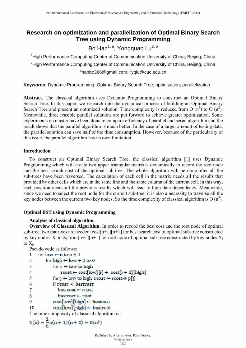
Analysis of Data Correlation. The dynamic process of constructing an optimal sub-tree is shown in Fig.1:

The order of calculated results is ：A1→B1→B2→C1→C2→C3→…→G5→G6→G7. Take G7 for example, it depends on the other results which are in the same row: G1, G2 … G8 and

same column: F6, E5, D4 … A1.

In the same way, G6 needs the results of F5, E4, D3…B1. In this way, we could know that G7

needs all the other results generated in the upper triangular matrix. From the above analysis, we can conclusion that this Dynamic Programming algorithm hs strong data dependency and low parallelism.

Parallel solutions.

Cell data into parallel. On account of the strong data dependency, we consider to parallel this process for each cell in the matrix. According to the classic algorithm, records the best cost

0230



of a optimal sub-tree constructed by key nodes to . Traversing every node between and is required for each calculation, as a result, the parallelization processing can be achieved by broking down the traversing process to different processors.

In this solution, the calculation of each cell of the upper triangular matrix requires one MPI_Allreduce and MPI_Bcast. Suppose the number of key nodes is n and the number of processes is m, so the communication complexity is:

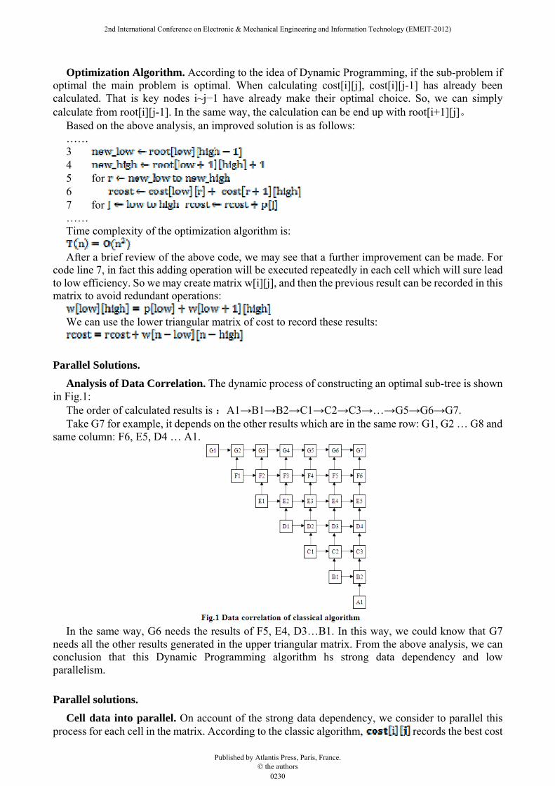
Paralleling by diagonal. In fact, the results of main diagonal line have already known which the

search probabilities of all those key nodes are. Because of this, we can fill the matrix diagonal by diagonal. The results in the same diagonal can be calculated independently. Then these calculation tasks will be distributed to different processors. (Fig.2)

In this solution, all processors need one MPI_Allreduce communication for each diagonal, so that

n times of communication is in total. The communication complexity is：

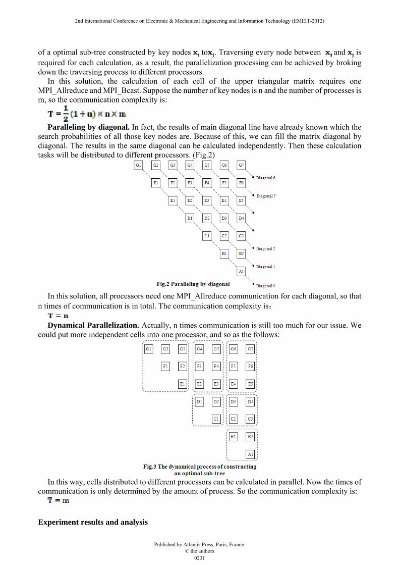
Dynamical Parallelization. Actually, n times communication is still too much for our issue. We

could put more independent cells into one processor, and so as the follows:

In this way, cells distributed to different processors can be calculated in parallel. Now the times of

communication is only determined by the amount of process. So the communication complexity is:

Experiment results and analysis

0231



Programs run on Symmetrical Multi-Processing cluster with X86 GNU/Linux core, Intel(R) Xeon(TM) 3.80GHz CPU. The number of processors is 24*2 with 8182344KB memory.

Comparision of classical and optimization algorithm. The number of testing key nodes is: 0, 50, 100, 200, 300,400 and 500. The test result is shown in Table 1.

Table 1 Comparison of classical and optimization algorithms

The testing result shows that because of the reduction of inner loop and record of intermediate

results, unnecessary calculation has been eliminated. With the increasing amount of testing data, the execution time of classical algorithm was close to the exponential increase .However, execution time of the program using improved algorithm changed a little with the same amount of testing data. The performance of optimized algorithm improved significantly.

Comparison of optimization and parallel algorithm. The number of testing key nodes is: 1000, 5000, 10000, 15000 and 20000. The test result is shown as Table 2.

Table 2 Comparison of parallel algorithms

It isn’t hard to tell from the above diagram that the frequency of communication of the first two

methods is determined by n. With the increasing of testing key nodes, their communication time is far beyond calculation time. But the third parallel method depends only on the number of processes.

Table 3 Comparison of serial and parallel algorithm

As is seen from the above diagram, the execution time of the third algorithm is longer than that of

serial algorithm when the amount of testing data is not large enough because the cost of

0232



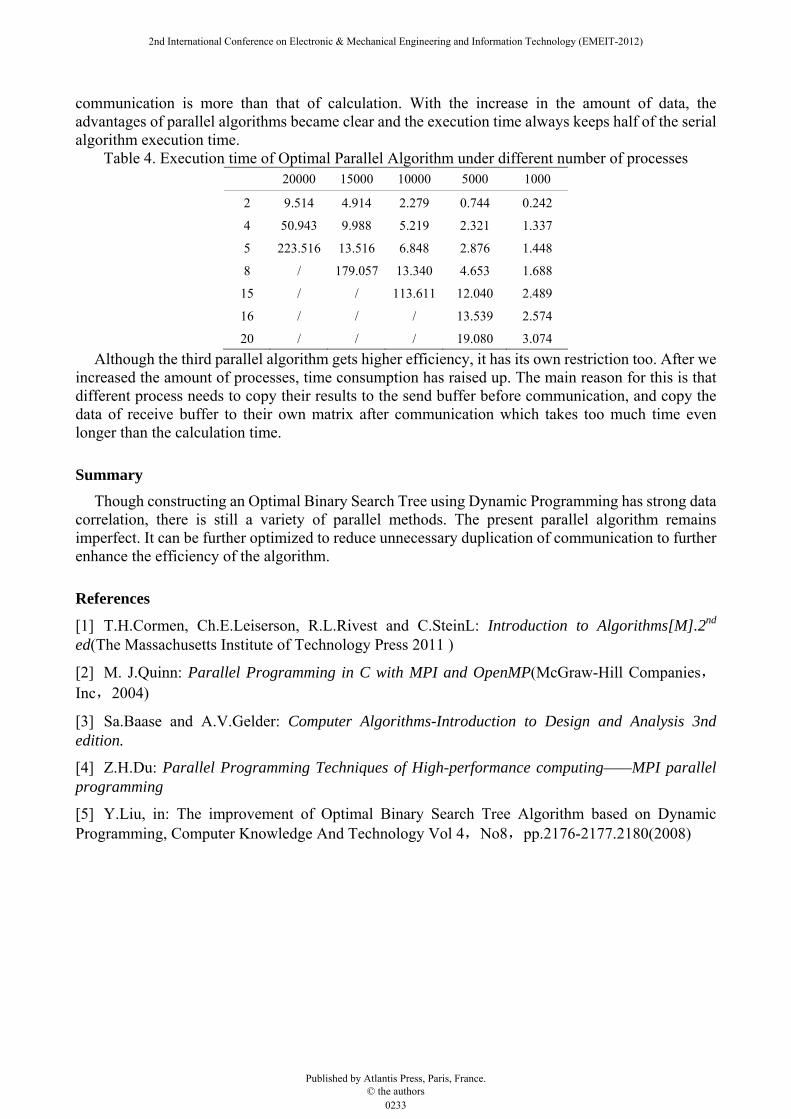
communication is more than that of calculation. With the increase in the amount of data, the advantages of parallel algorithms became clear and the execution time always keeps half of the serial algorithm execution time.

Table 4. Execution time of Optimal Parallel Algorithm under different number of processes 20000 15000 10000 5000 1000

2 9.514 4.914 2.279 0.744 0.242

4 50.943 9.988 5.219 2.321 1.337

5 223.516 13.516 6.848 2.876 1.448

8 / 179.057 13.340 4.653 1.688

15 / / 113.611 12.040 2.489

16 / / / 13.539 2.574

20 / / / 19.080 3.074

Although the third parallel algorithm gets higher efficiency, it has its own restriction too. After we increased the amount of processes, time consumption has raised up. The main reason for this is that different process needs to copy their results to the send buffer before communication, and copy the data of receive buffer to their own matrix after communication which takes too much time even longer than the calculation time.

Summary

Though constructing an Optimal Binary Search Tree using Dynamic Programming has strong data correlation, there is still a variety of parallel methods. The present parallel algorithm remains imperfect. It can be further optimized to reduce unnecessary duplication of communication to further enhance the efficiency of the algorithm.

References

[1] T.H.Cormen, Ch.E.Leiserson, R.L.Rivest and C.SteinL: Introduction to Algorithms[M].2nd ed(The Massachusetts Institute of Technology Press 2011 )

[2] M. J.Quinn: Parallel Programming in C with MPI and OpenMP(McGraw-Hill Companies，Inc，2004)

[3] Sa.Baase and A.V.Gelder: Computer Algorithms-Introduction to Design and Analysis 3nd edition.

[4] Z.H.Du: Parallel Programming Techniques of High-performance computing——MPI parallel programming

[5] Y.Liu, in: The improvement of Optimal Binary Search Tree Algorithm based on Dynamic Programming, Computer Knowledge And Technology Vol 4，No8，pp.2176-2177.2180(2008)

0233



Documents

Research on optimization and parallelization of Optimal