Embed Size (px)
Citation preview

AD 7 23 397
TECHNICAL R EPO R T NO. 6
STATIC AND DYNAMIC ANALYSIS OF ROCK BOLT SUPPORT
RESEARCH ONROCK BOLT REINFORCEMENT
RICHARD E. G OO DM A N AND JA C Q U E S D U BO IS
O M A H A DISTRICT, CORPS OF E N G I N E E R S O M A H A , N E B R A S K A 68102
THI S R E S E A R C H WA S F U N D E D BY O F F I C E , C HI E F OF E N G I N E E R S , D E P A R T M E N T OF T H E A R M Y
PREPARED UNDER CONTRACT DACA45-67-C-0015 MOD. P 0 0 2
by
■J A N U A R Y 1971
mm gw»?
BY THE UNIVERSITY OF CAL IFORNIA , BER KELEY , CALIFORNIAI
.W 3 ¿ ím^6< 9 71 A p p r o v e d fo r p u b l i c r e l e a s e ; d i s t r i b u t i o n u n l i m i t e d
BUREAU OF RECLAMATION LIBRARY DENVER, CO
Destroy this report when no longer needed.
Do not return it to the originator.
The findings in this report are not to be construed as
an official Department of the Army position unless
so designated by other authorized documents.
BUREAU OF RECLAMi
9207Í
IRARY
60
TECHNICAL REPORT NO. 6
STATIC AND DYNAMIC ANALYSIS OF ROCK BOLT SUPPORT^
RESEARCH ON ROCK BOLT REINFORCEMENT
^ by
RICHARD E. GOODMAN AND JACQUES DUBOIS f
y JANUARY 1971 V
OMAHA DISTRICT, CORPS OF ENGINEERS OMAHA, NEBRASKA 68102
THIS RESEARCH WAS FUNDED BY OFFICE, CHIEF OF ENGINEERS, DEPARTMENT OF THE ARMY
PREPARED UNDER CONTRACT DACAU5-67-C-0015 MOD. P002 BY THE UNIVERSITY OF’d ALIFORNIA^ BERKELEY^ CALIFORNIA
Approved for public release, distribution unlimited.
92073860

STATIC AND DYNAMIC ANALYSIS OF ROCK BOLT SUPPORT
ABSTRACT
This report describes progress in a continuing effort to develop and
evaluate methods which can be used to design underground openings to sur
vive blast loadings. It includes discussion of the action of rock bolts
Under static loads and considers aspects of the interaction between rock
and rock bolt under dynamic loads. Only computational methods were used
in this study.
| First, closed form solutions for point loads are summed and superim
posed to examine stresses induced by patterns of rock bolts around tunnels
in linearly elastic material. The stress fields are compared to rock
strengths according to simplified failure criteria, to appreciate the
relative strengthening effect of different combinations of bolt and rock
parameters. It was found that very substantial bolt pressures are required,
e.g. 10% of the maximum applied pressure, to restrict rock breakage in
ideally elastic material.
Then elastic-plastic material behavior is considered. Stresses in
duced by unequilibrated line loadings on the inner circumference of the
tunnel are used to simulate rock bolt patterns. It is found that the rock
bolt strengthening effect can more easily be substantiated in weaker
materials. For example, when rock inside the "plastic" zone was taken as
cohesionless, less than 1% of the blast pressure is a sufficiently high
rock bolt pressure to provide significant strengthening effect.
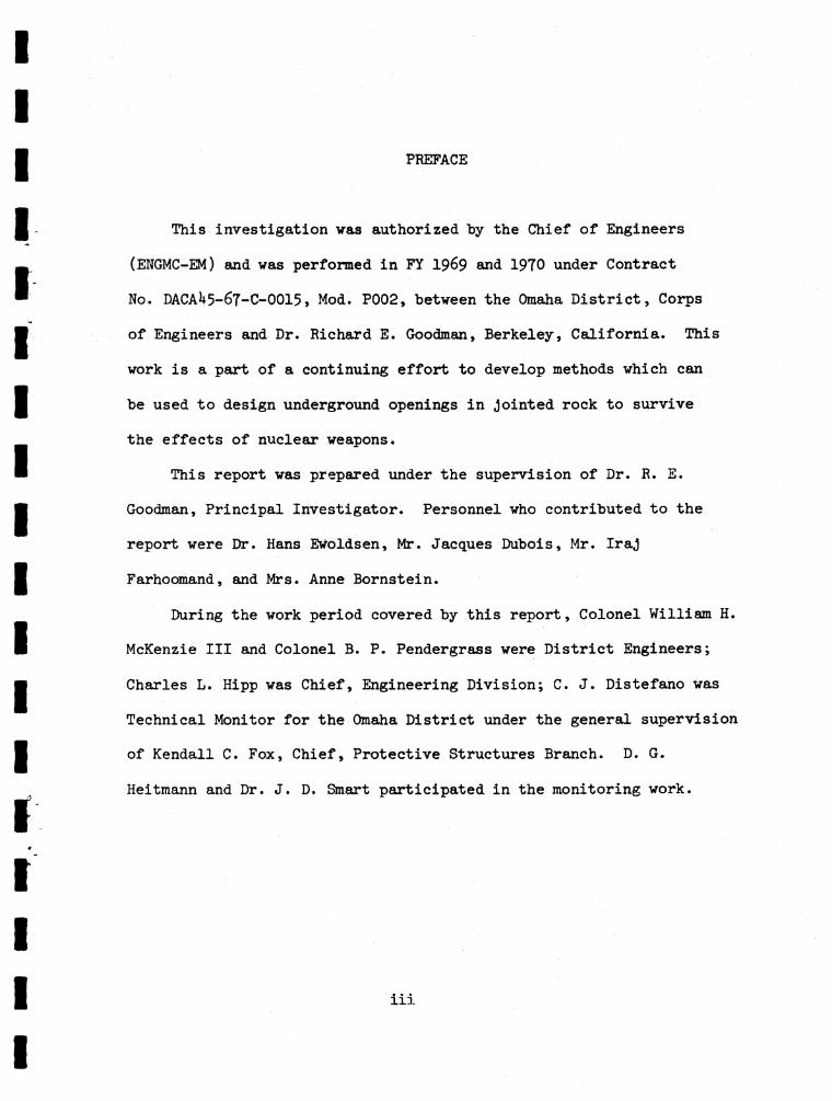
Dynamic considerations are discussed in terms of an energy balance
for the case of a plane rock wall bolted in a regular pattern which receives
a stress wave impulse from inside. The problem is examined in two ways:
First a calculation is made of the kinetic energy of the system in thei
most serious increment of time during the response, assuming the bolt to
behave elastically. Then, the total work during all of the blast response
period is considered, presuming the bolt damage to be cumulative. The
objective of these computations is to provide a basis for scaling sur
vivability conclusions from one experiment to another. Reference is made
to Hardhat and Piledriver experiments.
ii
PREFACE
This investigation was authorized by the Chief of Engineers
(ENGMC-EM) and was performed in FY 1969 and 1970 under Contract
No. DACAU5-67-C-OOI5, Mod. P002, between the Omaha District, Corps
of Engineers and Dr. Richard E. Goodman, Berkeley, California. This
work is a part of a continuing effort to develop methods which can
be used to design underground openings in jointed rock to survive
the effects of nuclear weapons.
This report was prepared under the supervision of Dr. R. E.
Goodman, Principal Investigator. Personnel who contributed to the
report were Dr. Hans EWoldsen, Mr. Jacques Dubois, Mr. Iraj
Farhoomand, and Mrs. Anne Bornstein.
During the work period covered by this report, Colonel William H.
McKenzie III and Colonel B. P. Pendergrass were District Engineers;
Charles L. Hipp was Chief, Engineering Division; C. J. Distefano was
Technical Monitor for the Omaha District under the general supervision
of Kendall C. Fox, Chief, Protective Structures Branch. D. G.
Heitmann and Dr. J. D. Smart participated in the monitoring work.
iii
TABLE OF CONTENTS
ABSTRACT----------------------------------------------------------- i
PREFACE------------------------------------------------------------ iii
NOTATION------------ viii
CONVERSION FACTORS, BRITISH TO METRIC UNITS OF MEASUREMENT------- xi
CHAPTER 1 INTRODUCTION---------------------------------------— 1
CHAPTER 2 AN ELASTIC APPROACH FOR DESIGN OF PATTERNED ROCK BOLTSUPPORTS UNDER STATIC OR QUASI-STATIC LOADING--------- 3
2.1 Approach--------------------------------------------------- * 32.2 Global Stress Field Around the Tunnel - Elastic Behavior— 52.3 The Extent of the Slip Zone---- --- 82.1+ Calculation of Rock Loads--------------------------------- 92.5 The Principle of the Design Method---------------- 102.6 Illustrative Example----------------------- 112.7 Conclusion---------- 13
CHAPTER 3 DESIGN APPROACH FOR ELASTIC-PLASTIC ROCK UNDERHYDROSTATIC LOADING----- ----------------------------- 55
3.1 Mathematical Conditions------------------------------------ 553.2 Solution for Stresses and Extent of Plastic Zone----------- 573.3 Examples------------------------------------------- ■-------- 6l
3.3.1 Example No. 1------------------------------------------ 633.3.2 Example No. 2------------------------------------------ 63
3.1+ Conclusions------------------------------------------------ 6k
CHAPTER 1+ DYNAMIC ANALYSIS OF THE TUNNEL SUPPORT PROBLEM------- 86
l+.l Introduction---------------------------------------- ---- -— 86k.2 Rigid Two Body Analysis------------------------------------ 871+.3 Elastic - Two Body Analysis------------------------------- 891+.1+ Energy Approach to Rock Bolt Problem---------------------- 90
l+.l+.l Case 1: Only Kinetic Energy Considered----------------- 921+.J+.2 Case 2: Total Work Considered------------------------ 99
1*.5 Discussion--------------------------------- 102
CHAPTER 5 EMPIRICAL APPROACH TO SUPPORT DESIGN AGAINSTBLASTS---------- 110
5.1 Definitions---- •------------------------------------------- 1105.1.1 Wave Travel Time------------------ 1105.1.2 Energy Absorption by the Support System--------------- 1115.1-3 Energy Dissipation Time of the Support System--------- 112
iv
5.2 Results of the Pile Driver Tests--------------------------- 1125.2.1 General Empirical Energy Equation------------------------ 1135.2.2 Application to Pile Driver Test------------------------ 115
5-3 Hardhat Drift---------- ----------------------------------— 1175 .1+ Conclusion--------------------------------------------- ---- 118
REFERENCES-------------------------------------------------- 119
APPENDIX I------------------------- 120
APPENDIX II— ----------------------------------------------------- 127
v
TABLES
2 .1 Economic Comparison of Rock Bolt Design------------------- 162.2 Comparison of Rock Bolt Design I--------------------------- 172.3 Comparison of Rock Bolt Design II---------------------- 183.1 Radius of 3he Plastic Zone for Various Rock Properties_— 663.2 Variation of the Plastic Zone with C--------------- 663.3 Example No. 1 Results------------------ 66
FIGURES
2 .1 Stresses Due to a Single Rock Bolt--- — ______ 192.2 Comparison of Stresses with Failure Criterion________._____ 202.3a Joint Influence Diagrams for Case (SlAl) - Horizontal
Joint------------------------------------------------------- 212.3b Joint Influence Diagrams for Case (SlAl) - 30° Joint_______ 222.3c Joint Influence Diagrams for Case (SlAl) - 60° Joint_______ 232.3d Joint Influence Diagrams for Case (SlAl) - Vertical
Joint-------- ¿k2.k& Joint Influence Diagrams for Case (S1A2) - Horizontal
Joint------------------------------------------------------- 252.4b Joint Influence Diagrams for Case (S1A2) - 30° Joint------- 262.4c Joint Influence Diagrams for Case (S1A2) - 60° Joint____ 272.4d Joint Influence Diagrams for Case (S1A2) - Vertical
Joint— ---------------------- 282.5a Joint Influence Diagrams for Case (S1A3) - Horizontal
Joint------------------------------------------------------- 292.5b Joint Influence Diagrams for Case (S1A3) - 30° Joint______ 302.5c Joint Influence Diagrams for Case (S1A3) - 60° Joint______ 312.5d Joint Influence Diagrams for Case (S1A3) - Vertical
Joint---------------------------------- 322.6a Joint Influence Diagrams for Case (S3A2) - Horizontal
Joint------------------------------------------------------- 332.6b Joint Influence Diagrams for Case (S3A2) - 30° Joint------ 342.6c Joint Influence Diagrams for Case (S3A2) - 60° Joint_____ 352.6d Joint Influence Diagrams for Case (S3A2 ) - Vertical
Joint------------ 362.7a Joint Influence Diagrams for Case (S3A3) - Horizontal
2 .7b Joint Influence Diagrams for Case (S3A3) - 30° Joint----- 382.7c Joint Influence Diagrams for Case (S3A3) - 60° Joint----- 392.7d Joint Influence Diagrams for Case (S3A3) - Vertical
Joint------- ------------------------------------ -----------2.8a Joint Influence Diagrams for Case (L2A1) - Horizontal
Joint-----------— ------------------------------------ ----- 1 22.8b Joint Influence Diagrams for Case (L2A1) - 30° Joint_____ 422.8c Joint Influence Diagrams for Case (L2A1) - 60° Joint_____ 432.8d Joint Influence Diagrams for Case (L2A1) - Vertical
Joint__________ k4
vi
2.9a Joint Influence Diagrams for Case (L2A2) - HorizontalJoint---------------------------------------------- 1+5
2.9b Joint Influence Diagrams for Case (L2A2) - 30° Joint------ 1*62.9c Joint Influence Diagrams for Case (L2A2) - 60° Joint------ 1*72.9J Joint Influence Diagrams for Case (L2A2) - Vertical
Joint— •---------------------------------------------------- 1*82.10a Joint Influence Diagrams for Case (L2A3) - Horizontal
Joint— ---- 1+92.10b Joint Influence Diagrams for Case (L2A3) - 30° Joint--- - 502.10c Joint Influence Diagrams for Case (L2A3) - 60° Joint---- 512.10d Joint Influence Diagrams for Case (L2A3) - Vertical
Joint--------- 522.11 The Rock Load--------------------- •------ ---------- :-------- 532.12 Required Ultimate Strength for Rock Bolt Support Scheme-- 5I*3.1 Plastic and Elastic Zones------------------------------ ■---- 673.2 Plastic Stress Criterion----------------------------------- 683.3 Peak and Residual Strength---------------- 693.4 Equilibrium Diagram of an Infinitesimal Element------------ 703.5 Mohr Circle andFailure Characteristics 4>r» Cr , and <J>p, Cp 713.6 Mohr Circle and Failure Characteristics <|>r> Cr , and <}>p, Cp 723.7 Mohr Circle and Failure Characteristics <|>r , Cr , and (j>p, Cp 733.8 Mohr Circle and Failure Characteristics <f>r » Cr , and <J>p, Cp 7I*3.9 Radius of Destressed Zone---------------------------------- 753.10 Radius of Destressed Zone---------------------------------- 763.11 Radius of Destressed Zone---------------------------------- 773.12 Radius of Destressed Zone----------- 783.13 Radius of Destressed Zone---------------------------------- 793.11* Radius of Destressed Zone------------------------ 803.15 Effect of Rock Bolts on Stresses---------- 813.16 Effect of Rock Bolts on Stresses--------------------------- 823.17 Effect of Rock Bolts on Stresses--------------------------- 833.18 Effect of Rock Bolts on Stresses-------------------------- 8U3.19 Effect of Rock Bolts on Stresses--------------------------- 85l+.l Typical Wave Forms for Direct Transmitted Ground Shock
from Explosions---------------------------------------------- 10Uh.2 Model for Rigid Body Analysis-------------------------------1051+.3 Rock Bolt Tension and Plate Pressure Variation with Time— 106l+.U Momentum per Unit Area----------- 107U .5 Additional Energy in a Rock Bolt under an Initial Tension
T as a Result of Elastic Stretching------------------------1081+.6 Plastic Yield Energy Absorption by the Rock Bolt-----------109
vii
NOTATION
Angle between wave front normal and wall normal
%+ V% + *r/2Function of t^ and tg (eq h-22)
- Kinetic energy
erotal- energy associated with area A of wave front
er* - Proportion of energy associated with motion perp. to tunnel
eg« - Proportion of total energy associated with motion parallel totunnel
er - Proportion of er* that is not absorbed by the rock, or reflected, thus which goes to the rock bolts
erg - Maximum energy that can be absorbed by rock bolts
es - Proportion of er ' that is not reflected or absorbed by rock and therefore is directed to the supports (same as er if supports are rock bolts)
e0 ’ - Maximum value of er ' that can be withstood by a tunnel without support
eQ - e •' per unit area; = eo'/s^ for rock bolts spaced s feet
<j>p - Peak friction angle
<j>r - Residual friction angle
p - Mass density
o - Stress of elastic wave
ar - Radial stress
<jg - Tangential stress
Og - Bolt stress increment due to blast
a_ - Initial bolt stresss
viix
Tijc
eEF
k
KK
1
M-y
M
%
n
Stress tensor
Increment of strain to reach yield in a rock holt under initial strain
Polar coordinatesTransformation tensor-direction cosines between xyz, and x'y’z' axes
AreaCross-section area of rock bolt
Constant = 8q/i;
Constant defined by equation (5-*0
Residual cohesion
Peak cohesion
Phase velocity
Phase velocity of rock bolts
StrainElastic modulus of boltsForce of rock bolts necessary to prevent any displacement
Constant - see p. 78
Constant that is determined by boundary conditions
Constant - see p. 80
Length of rigid bodies in chapter 3} length of rock bolt in chapters H and 5
MassMomentum vector per unit area
Component of momentum vector parallel to tunnel wall
Component of momentum vector perpendicular to tunnel wall
R/(tdC)
ix
p - Hydrostatic pressure (external) due to rock stress or external loading
Pg - Average internal pressure on wall of tunnel due to bolting
R - Value of r at elastic - plastic boundary
R - Radius of tunnelo
R - Range — the distance to the blast point
S - Spacing between rock bolts on a regular pattern
T - Initial bolt tension
AT - Bolt tension increment due to blast
t„ - Transit time of stress wave in rock boltB CBt - Rise time of velocity pulse
td - Duration of positive phase of velocity pulse
U - Particle displacement
V - Particle velocity
V' - Particle velocity after impact (in rigid body analysis)
Xrb - Area under rock bolt stress-strain curve up to maximum allowablestress
x
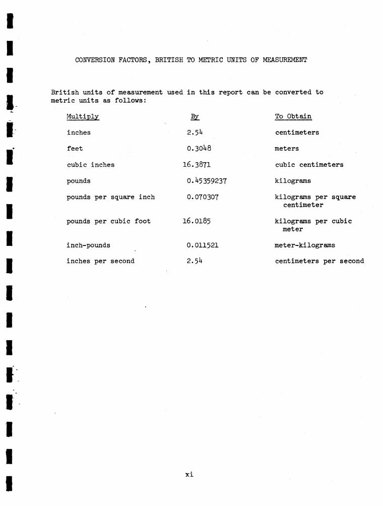
CONVERSION FACTORS, BRITISH TO METRIC UNITS OF MEASUREMENT
British units of measurement metric units as follows:
Multiply
inches
feet
cubic inches
pounds
pounds per square inch
pounds per cubic foot
inch-pounds
inches per second
used in this report can
Bj1
2 . 51*
0 . 3 0 U 8
16.3871
0.^5359237
0.070307
16.0185
0 .0 1 1 5 2 1
2.5^
be converted to
To Obtain
centimeters
meters
cubic centimeters
kilograms
kilograms per square centimeter
kilograms per cubic meter
meter-kilogr ams
centimeters per second
xi
CHAPTER 1
INTRODUCTION
In previous work, blast loading was approximated by a static
pressure, i.e., dynamic effects have been ignored. Support with rock
bolts, and with tunnel liners has been considered in particular
analyses; in addition, some basic analyses of rock bolt action were
pursued to gain an understanding of their action as structural
elements. All work has been in the framework of the Piledriver test,
that is, the underlying motive has been to obtain means for analyzing
rock performance in this test.
In this report, background gained in previous studies has been
brought to focus on the question of how to assign design parameters to
structural supports in tunnels subjected to static or dynamic loads.
First, the action of systematic bolting patterns is analyzed in
variably jointed rock masses assuming that elastic theory can be
applied. Then the case of systematic rock bolting of tunnels with a
"destressed" or "plastic" zone contained within an enveloping elastic
rock mass was considered. These first two approaches consider only
static or quasi-static loadings. The next approach attempts to
consider the dynamics of the support problem under impulsive loading.
Some of the ideas presented herein have not been tested in actual
experiments and this must be left to future studies to validate this
approach. The dynamic analysis presented is based on energy considera
tions and could be applied to tunnel liner design with some modifications.
Finally, the energy formulations are used to develop an empirical
equation for dynamic design of tunnel supports and evaluates the
constants of the equation from the results of the Piledriver test.

CHAPTER 2
AN ELASTIC APPROACH FOR DESIGN OF PATTERNED ROCK BOLT SUPPORTS
UNDER STATIC OR QUASI STATIC LOADING
2.1 APPROACH
The first uses of rock bolts were as dowels — passive
reinforcement in which the yield force of the bolts is available
as a reaction to rock load after approximately a tenth inch of
rock movement. Then pretensioning was added to bring the bolts
into their working range without additional rock movement. Many
convincing demonstrations and models entice the designer to specify
pretensioning but as yet there is no true understanding of rock
bolt behavior. Present design approach is generally based on
previous experience without a rational scheme for selecting the
principal parameters — length, spacing, prestress, and size of
rock bolts. Three theories have been advanced to try to explain
rock bolt action and to guide its design as rock reinforcement.
First, in laminated rock, the bolt stress is thought to increase
interlayer shear strength, thereby stiffening the roof into a load
carrying beam. Second, the radial confinement that is offered by
the average pressure supplied by the bolts raises the strength of
the rock around the gallery. Third, that rock bolts are depicted
as passive members preventing large deformations from destroying
the keying action of joint blocks.
Rock bolts are installed in the inner surface of an excavation
carved in an initially stressed body. At the time of installation
3
the stresses around the excavation approach the final values for
an unlined tunnel. Depending on the initial stress field, joints
in the rock, and the manner of excavation, the prebolting stress
state may approach the applicable elastic solution, eg. the Kirsch
solution for a circular tunnel, or may contain a destressed zone
of permanently deformed rock.
Some rock blocks fall out during excavation of the gallery or
remain suspended in a delicate equilibrium. Other blocks become
partially detached from the rock mass but remain entirely stable.
After installation of the rock bolts, the stress state may be
radically altered, as the bolts are tensioned to become active
structural partners with the rock. Finally, the rock in service
comes under additional live loads imposed by operation of the
gallery and the stiffness of the remaining steel exercises a passive
resistance against further rock movements.
The proportion of the available steel area that should be
assigned to the contrasting active and passive roles depends on the
combination of geological conditions, prebolt installation stress
state, and post installation live loads. Each gallery is unique
and one cannot hope for a universal design. By combining solutions
to the relevant components of the total stress field and introducing
an appropriate criterion of failure, it is possible to compare the
relative merits of trial rock bolt designs. The individual compo
nents of the final stress state are the stresses imposed by the
anchor and plate of each rock bolt, the prebolting stress field
1IIIIIIIIaaa8IIIII
around the tunnel, and the stresses imposed by live loads. The
criterion of failure most appropriate to use is that describing the
slippage of rock blocks along jointing planes. Since the behavior of
jointed rock is nonlinear, and the installation is sequential, no
linear, elastic, one-step analysis cam reproduce rock bolt action.
Initial efforts to represent rock bolts in finite element analysis
were disappointing. Success is now being achieved using incremented
loading techniques using finite element programs which model joints
and bedding planes and which represent the excavation and construction
sequence. Still something may be learned from elastic solutions as
demonstrated below.
2.2 GLOBAL STRESS FIELD AROUND THE TUNNEL - ELASTIC BEHAVIOR
Many publications give stress fields about galleries subjected
to various load conditions. Exact solutions are available for
idealized tunnel shapes in isotropic and orthotropic plastic materials,
as well as for isotropic elastic-plastic materials. Heterogeneous
materials and complex tunnel shapes have been studied by photoelastic
techniques, as well as by use of the finite-element analysis. For
the purposes of this discussion, the starting point has been the well
known Kirsch solution (Ref. l) giving the stress field about a cir
cular gallery excavated in an initially stressed, linearly elastic,
homogeneous and isotropic medium.
Simulation of the loads imposed by the rock bolt is achieved by
superposition of the stress fields of two co-linear point loads, one
5
a surface loading representing the bolt bearing plate, the other an
interior point loading representing the rock bolt anchor. The first
point load solution is the familiar Boussinesq problem (Boussinesq,
1885); the second solution vas developed by Mindlin (1963). If
desired, a more exact simulation could be achieved through the
superposition of a surface plate loading solution and an interior
point load solution. Investigations have shown that for points of
interest removed from the immediate vicinity of the ends of the
bolt, use of the point load solution is sufficient. Ewoldsen
(Ref. 2) evaluated the error involved in using point loads on a half
space to represent rock bolts on the wall of a circular tunnel. In
effect the circular wall is being replaced by a series of planes
normal to each bolt. For an 8 bolt ring, of 10,000 pound preloaded
bolts in a tunnel 16 feet in diameter, the maximum error is of the
order of 0.5 psi.
The form of the stress component expressions resulting from
superposition of the two point load solutions is:
= P * f (Xi, L) (2-1)
Where:
P = bolt loading
Xi = coordinates of the point of interest referenced to the
bolt axis ^ta
L * length of bolt
Thus for an assumed bolt length, the stress field components
for a given bolt load may be obtained by multiplying previously
6
IIiIIIIy-v.
I111MIII1I
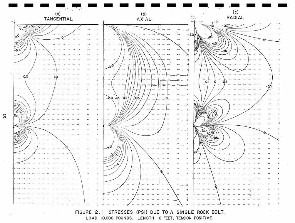
computed unit bolt load stresses by the given loading. Examples
of single rock bolt stress components are given in Figure 2.1.
In order to ascertain the global stress field existing around
the rock bolted tunnel, it is necessary to reference all stress
fields, tunnel and rock bolt, to a global coordinate system. Further,
components from individual bolts must be summed, and added to the
existing tunnel stress, at every point of interest in the global
coordinate system.
In the present example bolt stresses are initially referenced
to a cylindrical coordinate system whose axis is coincident with
the bolt axis. These bolt stresses are transformed through the use
of a second rank tensor transformation into components referenced to
the cylindrical tunnel coordinate system.
Tkl x AkiAlJTijWhere:
Amn « direction cosines between the two coordinate systems
k,l refer to tunnel coordinates
ij refer to bolt coordinates
Knowing the location and orientation of each bolt with respect to
the tunnel coordinate system, the stresses due to single bolts may
be summed since we are dealing with a linearly elastic, isotropic
medium-. This summation is accomplished by first finding the location
of the point of interest with respect to the individual bolt coordi
nate systems. This location will vary as the position and orientation
7
of each bolt with respect to the particular point is, in general,
not uniform. As the bolt stresses decrease radially as a function
of 1/r2 or greater, it is in general only necessary to consider
bolts lying within a 30° cone around a radial line from the tunnel
centerline through the point of interest. The transformed stress
components at the point contributed by the several bolts are then
summed. N
Where:
Tkl “ stress at a point due to n**1 bolt nH = total number bolts considered
The resultant multiple bolt stress field is then added to the
existing tunnel stress field.
Tkl * Vi +Tkl (2-4) total KXtunnel xrock boltsThe final transition to the desired global coordinate system is
accomplished through another second rank transformation.
Trs * Ltk.Asl\l (2-5)From this point, examination of the effects of the rock bolts under
various failure criteria is easily accomplished.
2.3 THE EXTENT OF THE SLIP ZONE
The criterion of failure adopted should reflect the way in
which the tunnel would behave if there should be no reinforcement.
In hard rock, the usual failure mode involves the relative movement
IIfI1
III1
IIIiII1
iI8
11IIItIIIIII1IIIi1
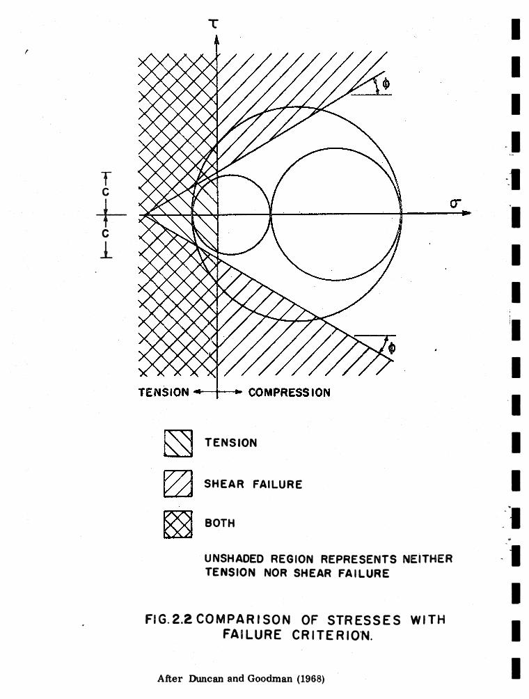
of blocks bounded by structural surfaces such as joints or bedding planes; therefore, in the illustrations presented here a criterion of failure has been selected in which the shearing strength of geological weakness planes is the sole consideration. Figure 2.2 portrays the failure criterion — a linear mohr envelope characterized by a cohesion and an angle of friction but with no tensile strength. Any stress field can be examined with such a failure criterion if
the orientations of weakness surfaces are specified.Examining each point around the tunnel in turn, it is possible
to identify the loci of points having a factor of safety of 1; any weakness surface of the given orientation passing through the locus will be critically stressed. Thus the whole region around the tunnel
is subdivided into subregions within which weakness surfaces of the given set are either over-stressed or under-stressed according to
the failure criterion. Actually no rock can be "over stressed" as the elastic stress distribution must give way to one which is everywhere acceptable. The scheme pursued here is simply a calcula
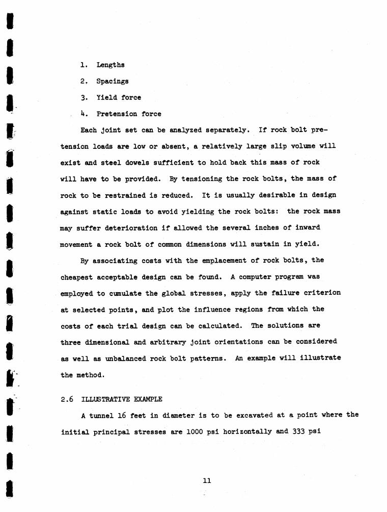
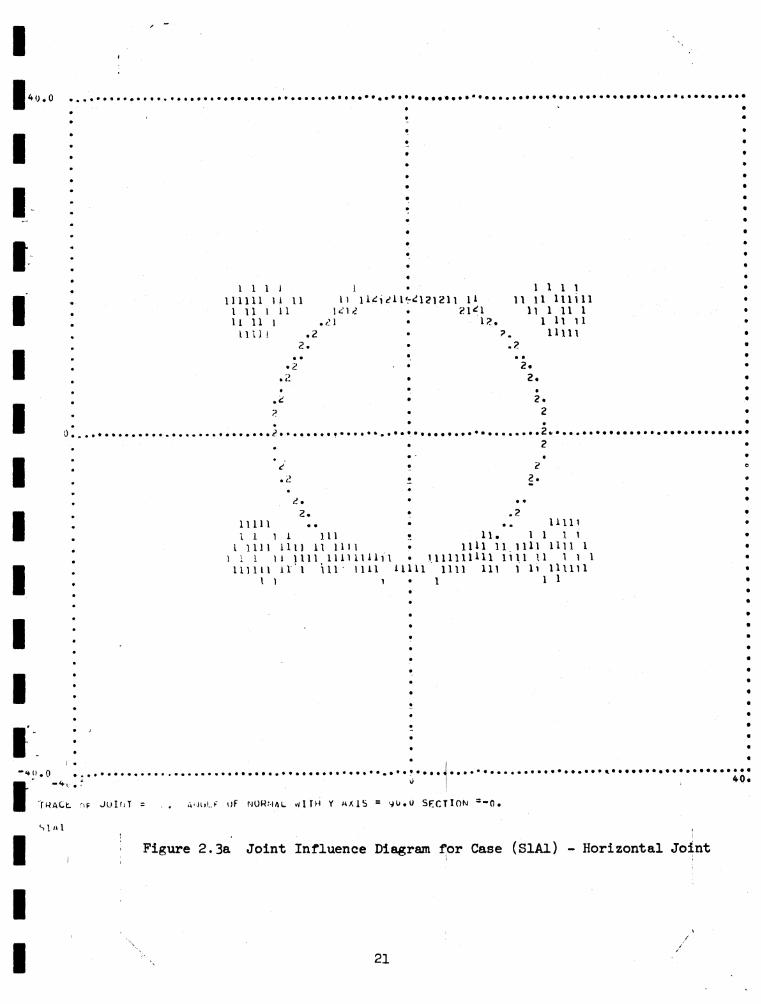
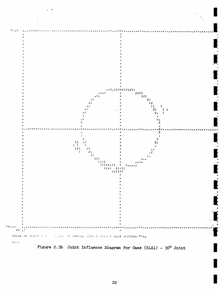
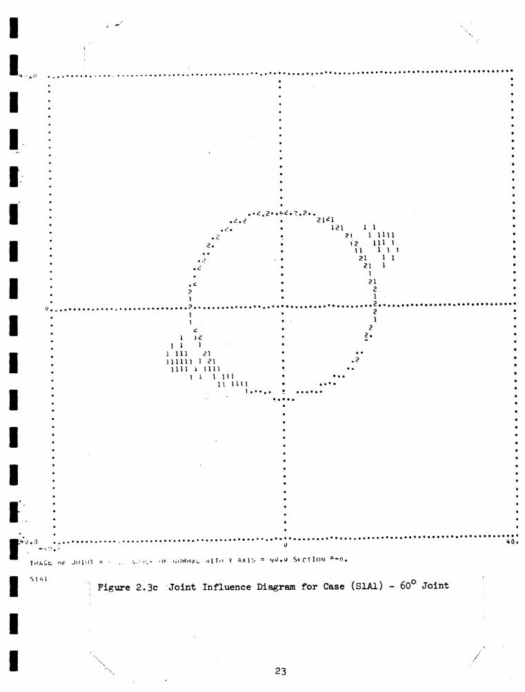
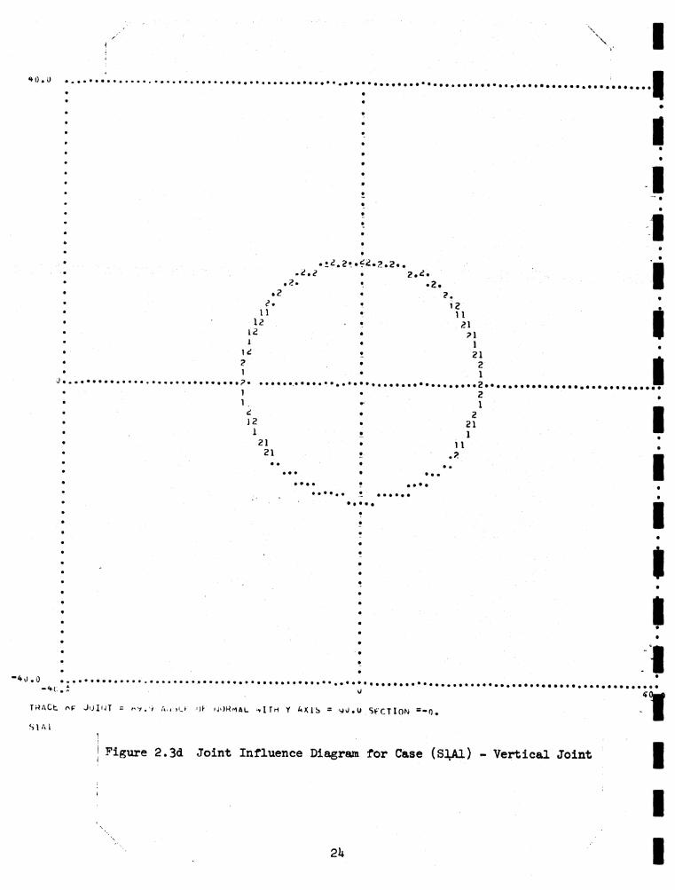
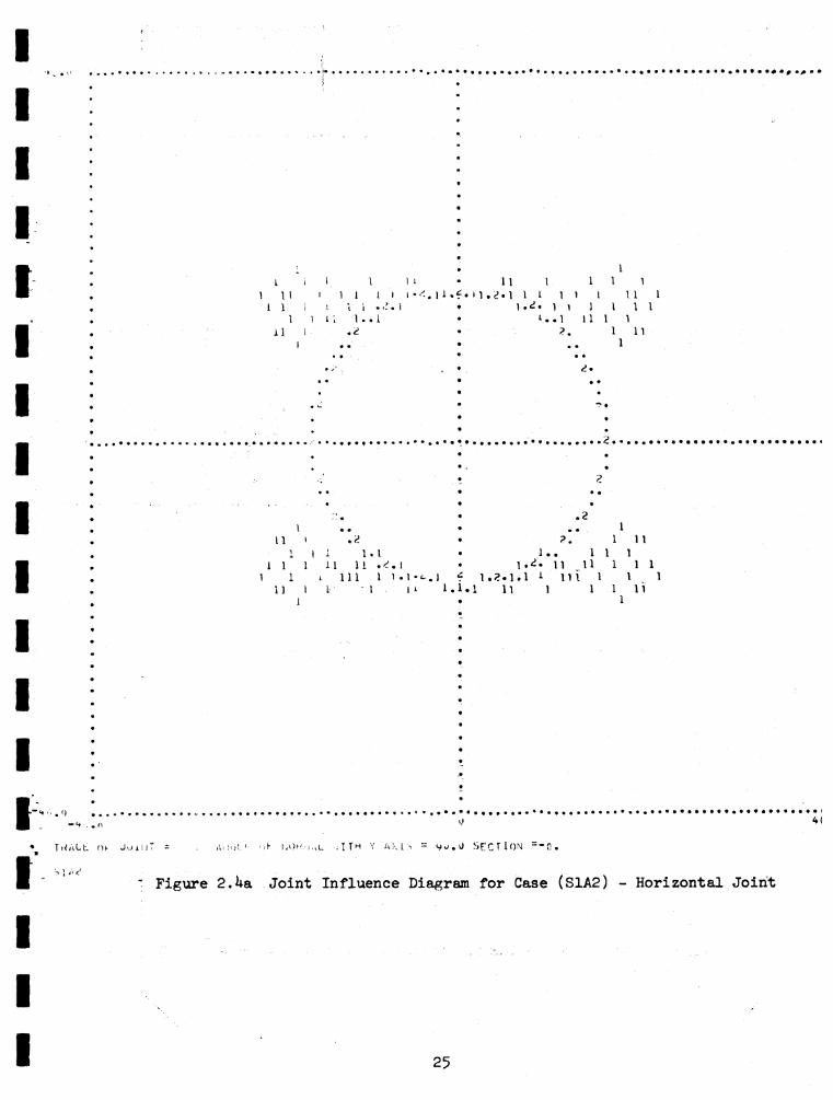
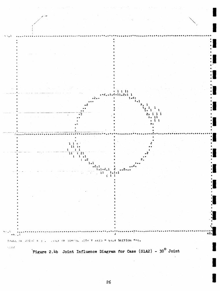
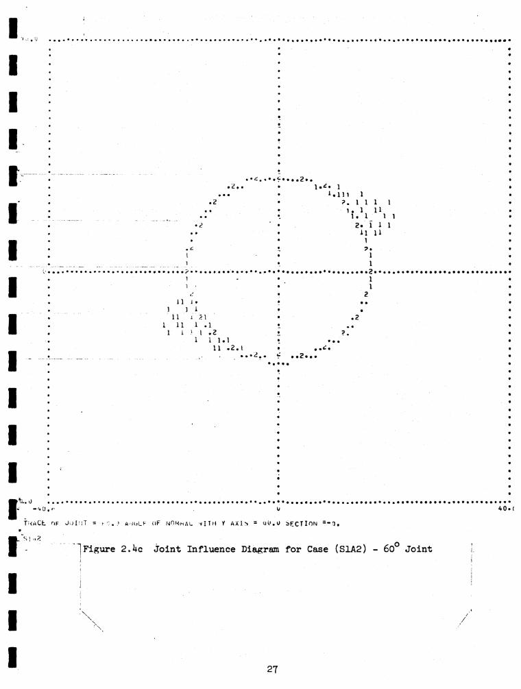
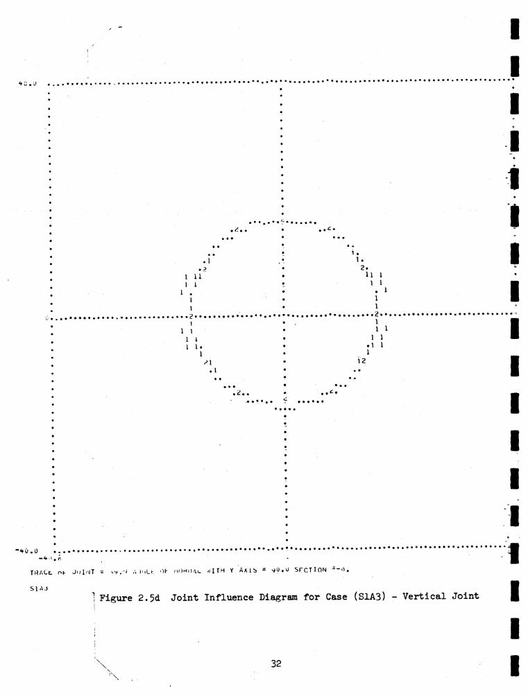
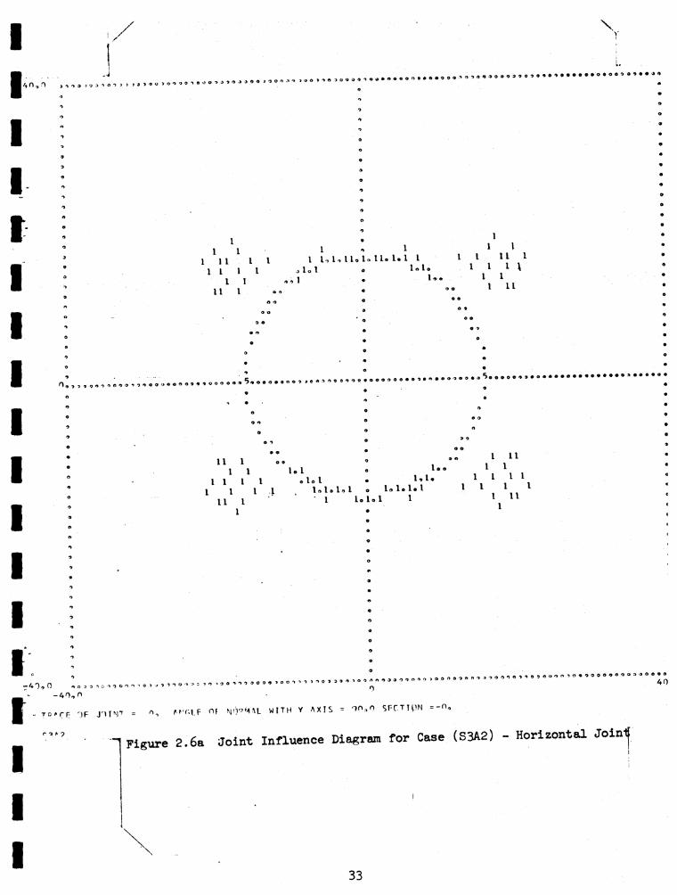
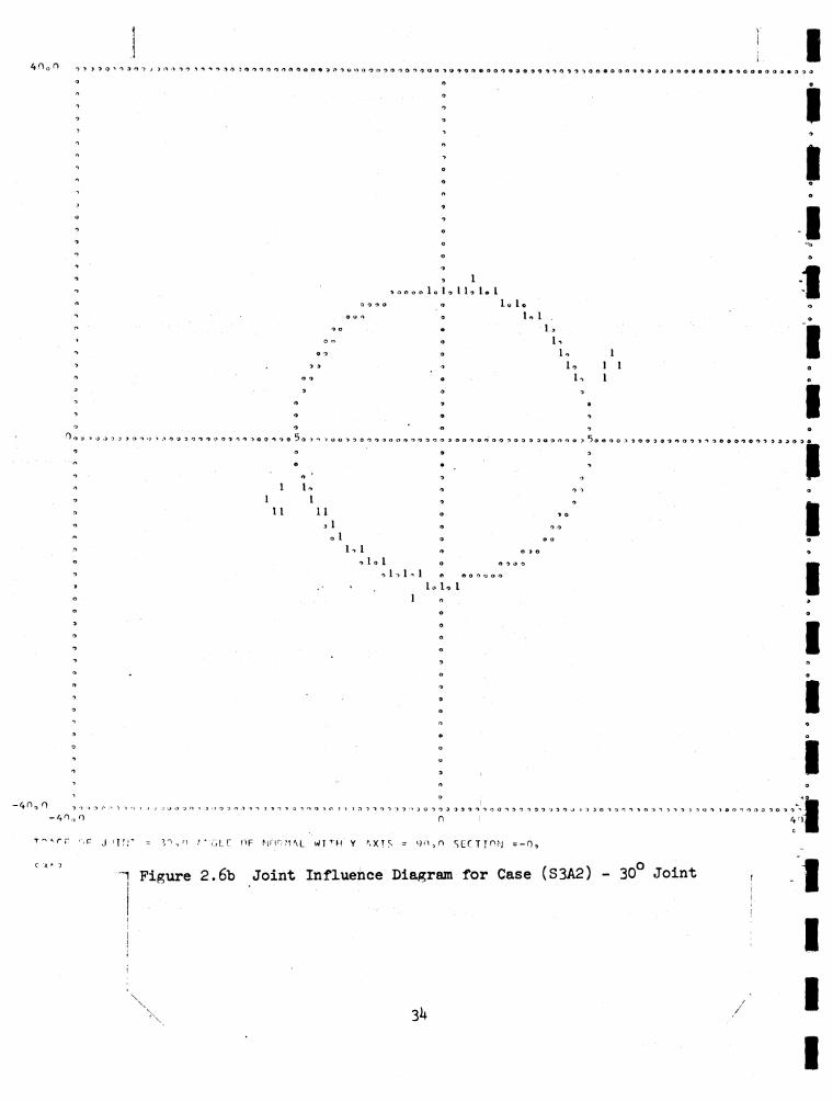
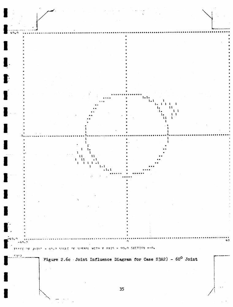
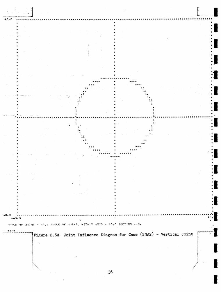
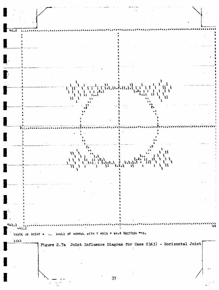
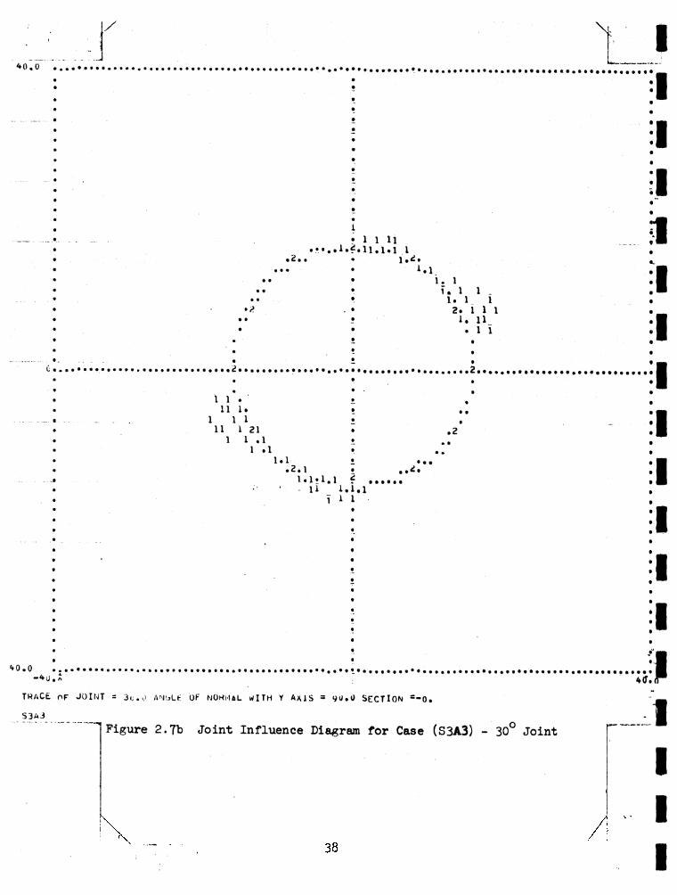
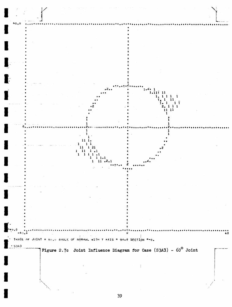
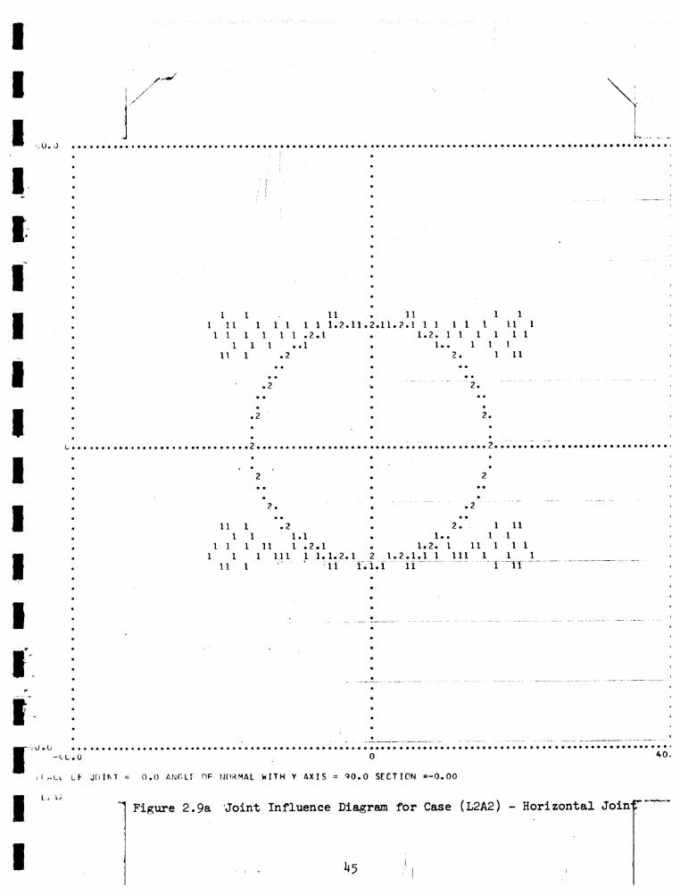
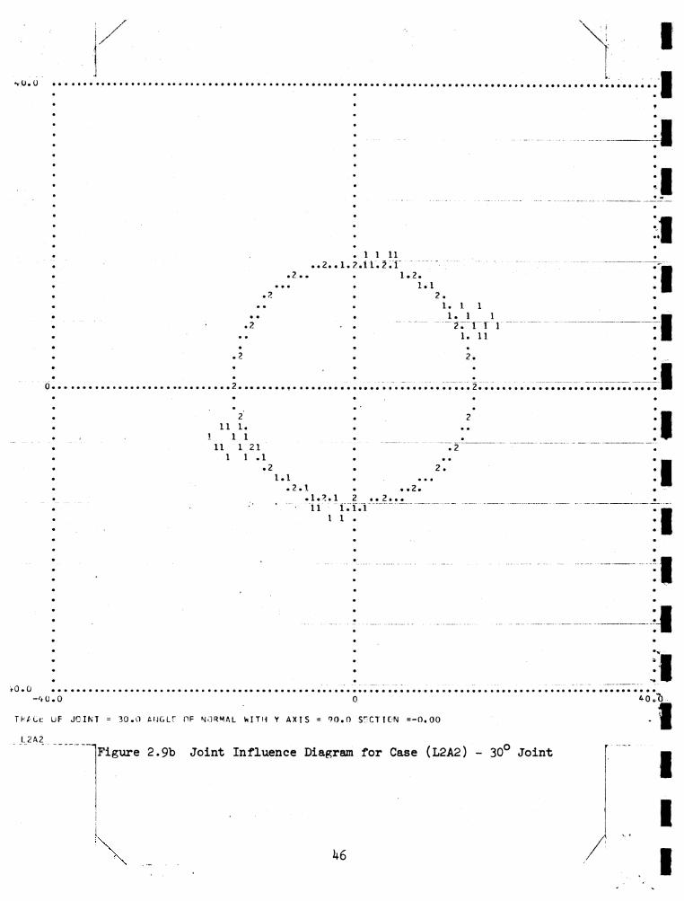
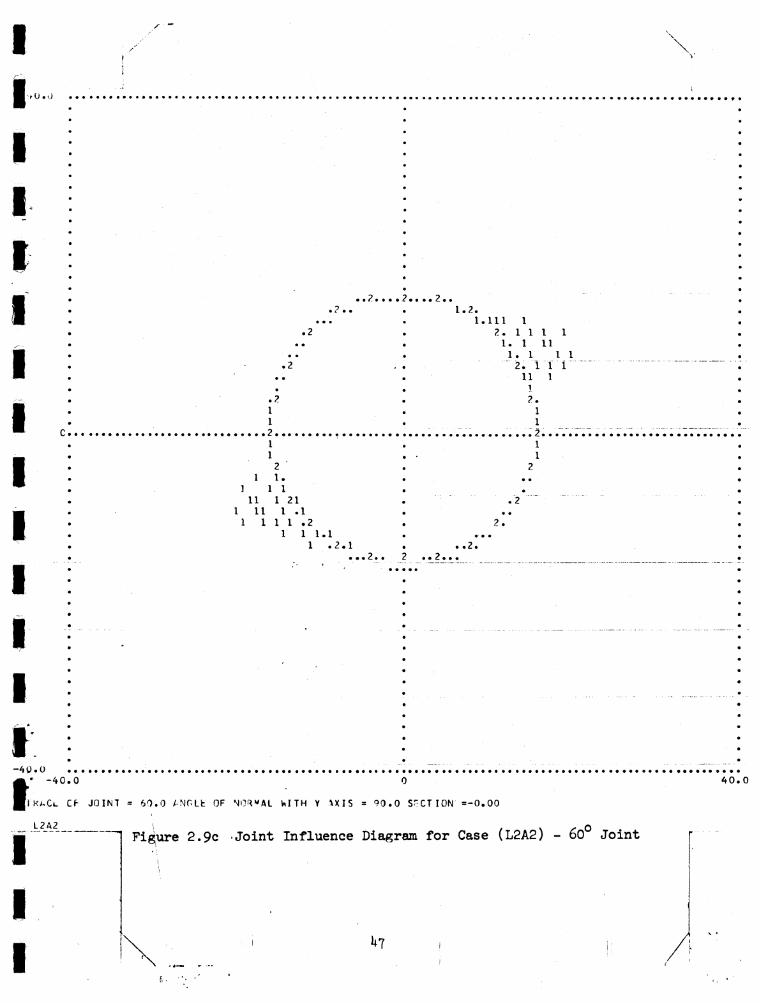
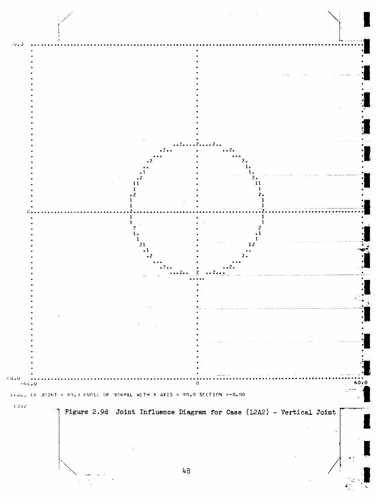
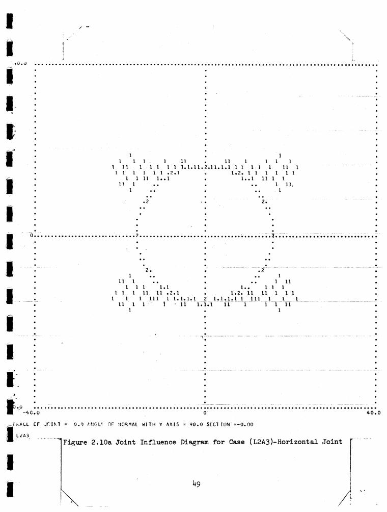
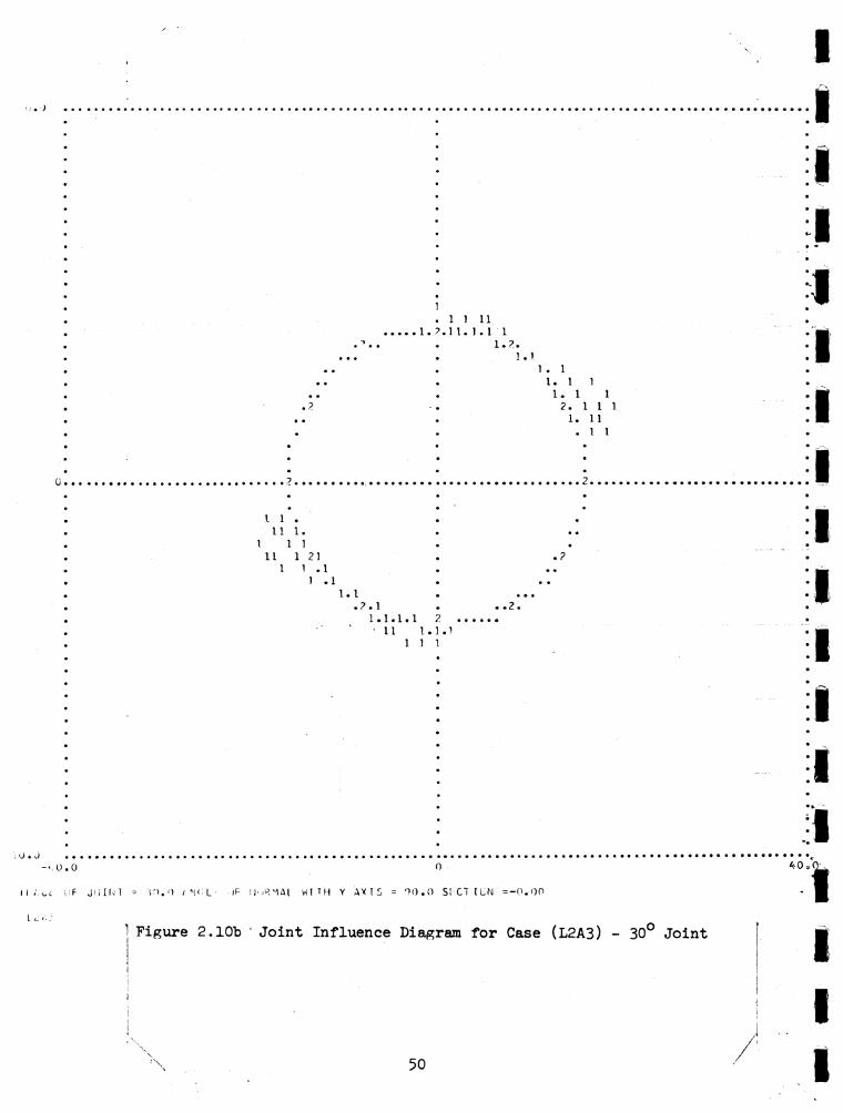
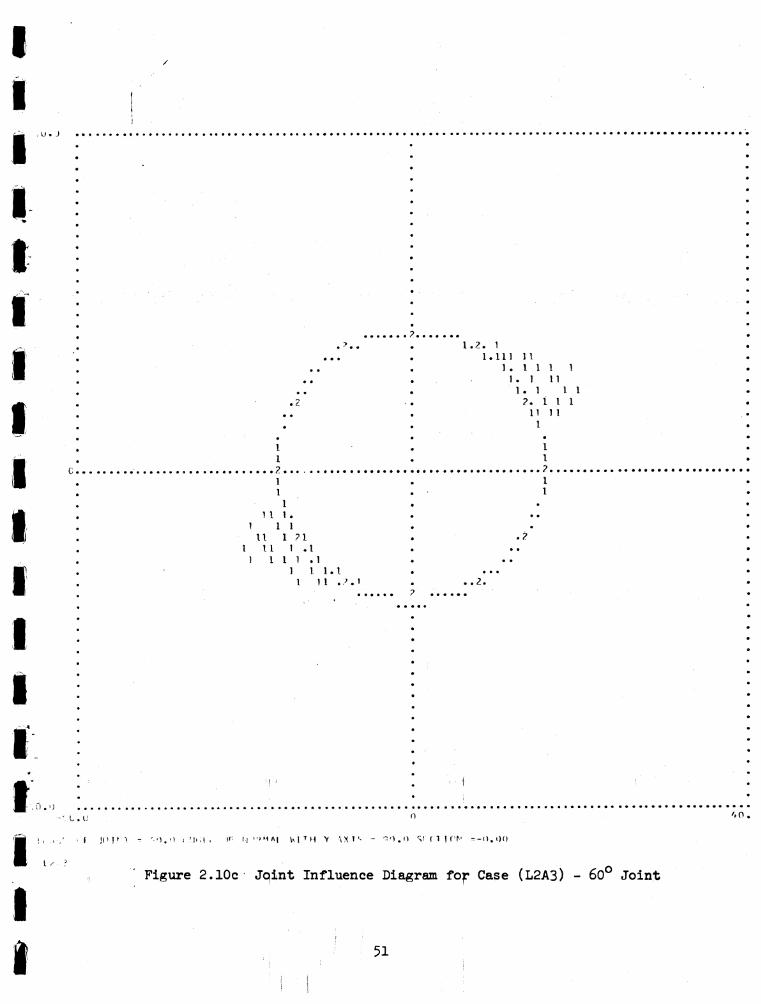
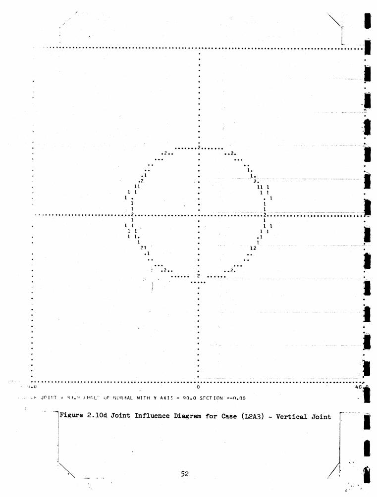
tion method making use of elastic stress distributions to estimate the maximum extent of rock requiring support. Figure 2.3-2.10
gives examples of such charts, which can be considered as joint influence diagrams to allow examination of the relative influence
of weakness planes at different positions near a tunnel.
2.1+ CALCULATION OF ROCK LOADSGravity urges the rock within the over-stressed subregions to
drop into the tunnel. An upper bound to the rock loads is therefore
9
calculated by establishing the mass of rock within the joint influence
areas. Above the tunnel, side restraint does not appreciably reduce
this load, whereas in the tunnel walls, the residual shear strength
along the joint orientation considered partially offsets the rock
load. Figure 2.11 illustrates the principle of calculation. The
rock bolts should be anchored behind the farthest extent of the
influence region. To provide an upper bound to the rock load per
bolt, it is calculated here as simply the wall area per bolt times
the maximum extent of the slip zone for any joint.
2.5 THE PRINCIPLE OF THE DESIGN METHOD
The object of the design is to achieve an optimum reduction of
the influence volume through prestressing the rock bolts, always
allowing sufficient reserve steel area to support the rock load with
the required factor of safety.
The following information must be known:
1. The diameter of the tunnel
2. The preferred orientation of each set of planar weaknesses
3. The cohesion and friction angle for each set of discontinu
ities
h. The initial principal, stresses near the tunnel
In seeking an optimum design, trial rock bolt parameters are
selected. The object is to specify the following parameters of the
rock bolts:
III1I
II888I8ft
1II810
IIII. IIVIIIIItII1II
1. Lengths
2. Spacings
3. Yield force
U. Pretension force
Each joint set can "be analyzed separately. If rock holt pre
tension loads are low or absent, a relatively large slip volume will
exist and steel dowels sufficient to hold hack this mass of rock
will have to he provided. By tensioning the rock holts, the mans of
rock to he restrained is reduced. It is usually desirable in design
against static loads to avoid yielding the rock holts: the rock mass
may suffer deterioration if allowed the several inches of inward
movement a rock holt of common dimensions will sustain in yield.
By associating costs with the emplacement of rock holts, the
cheapest acceptable design can he found. A computer program was
employed to cumulate the global stresses, apply the failure criterion
at selected points, and plot the influence regions from which the
costs of each trial design can he calculated. The solutions are
three dimensional and arbitrary joint orientations can be considered
as well as imbalanced rock holt patterns. An example will illustrate
the method.
2.6 ILLUSTRATIVE EXAMPLE
A tunnel 16 feet in diameter is to be excavated at a point where the
initial principal stresses are 1000 psi horizontally and 333 psi
11
vertically. The rock is divided by cohesionless Joints having a
friction angle of 50°. Establish the rock bolt design parameters.
Several trial designs are selected as listed in the four left
columns of Table 2.1, Part 1. The Joint influence diagrams for each
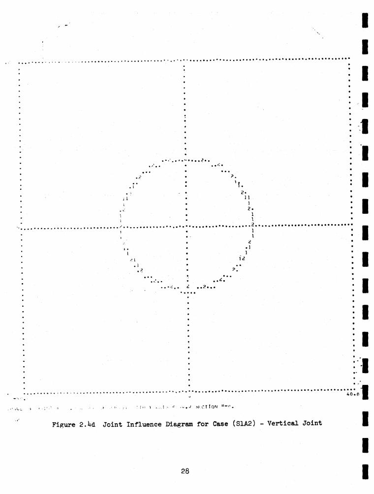
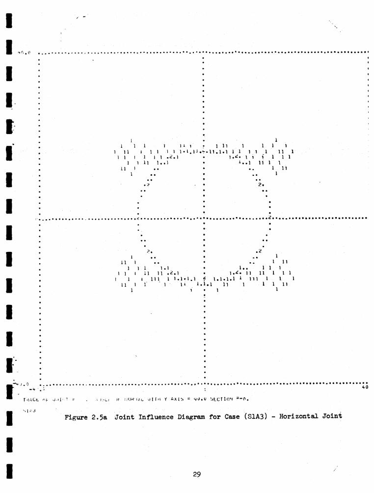
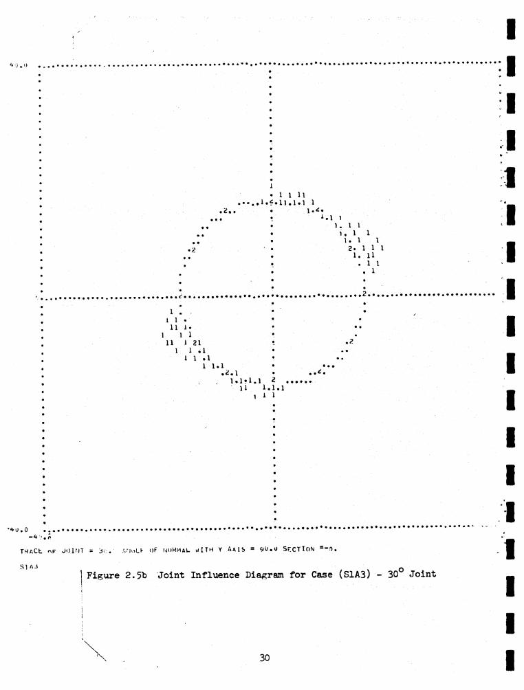
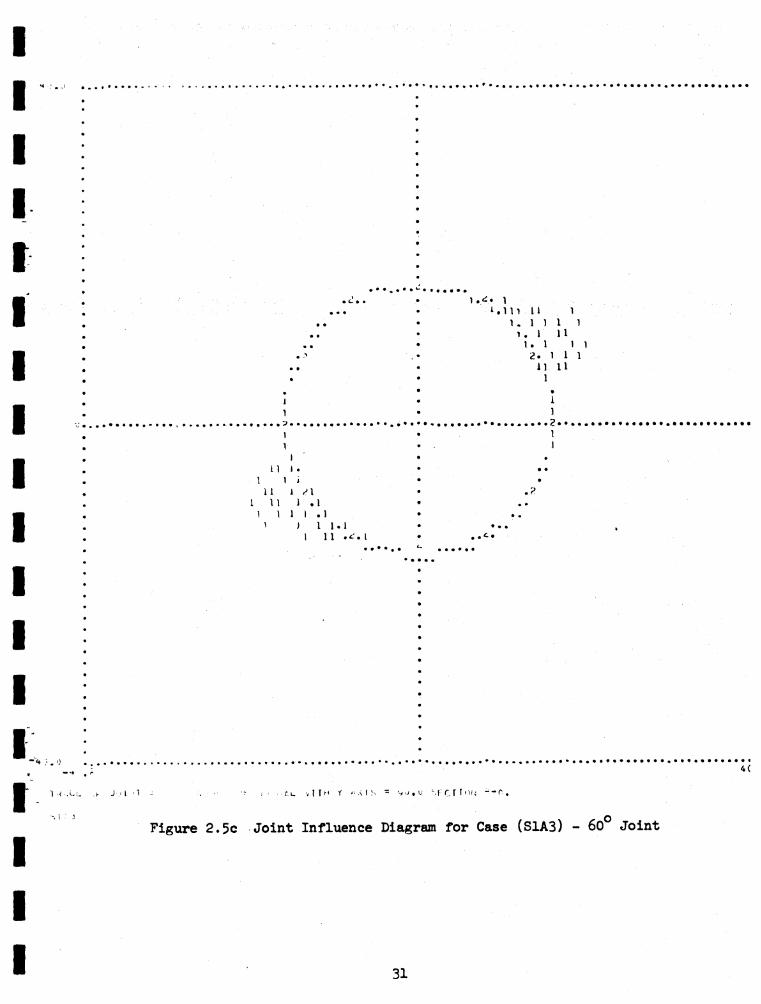
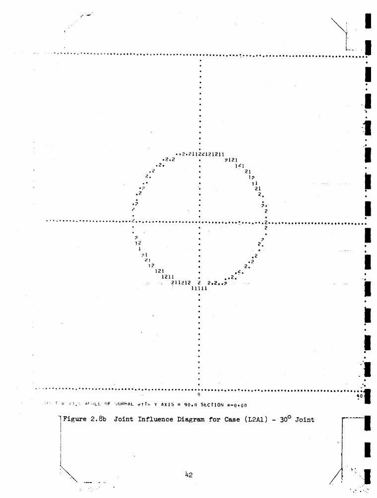
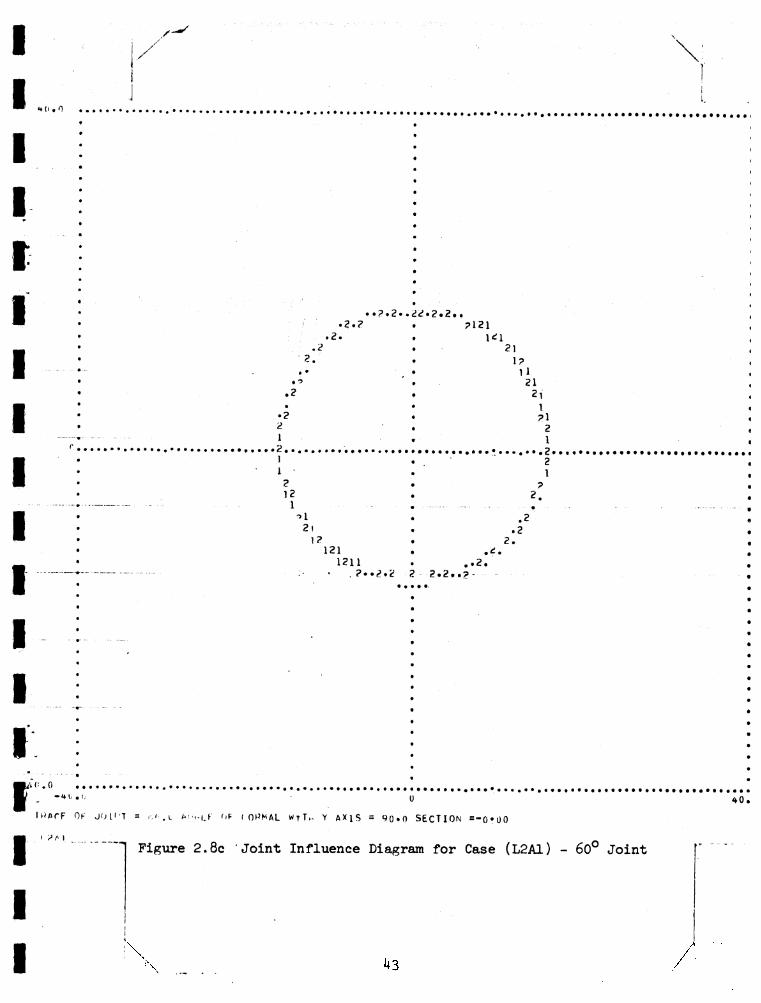
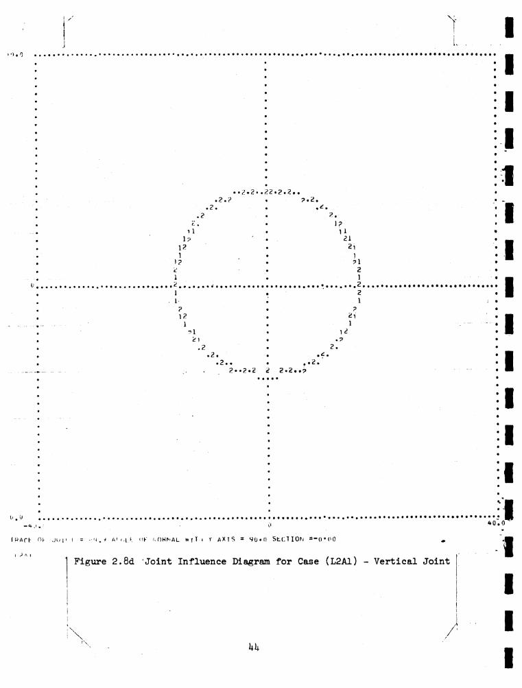
of the eight cases are presented in Figures 2.3-2.10. In these
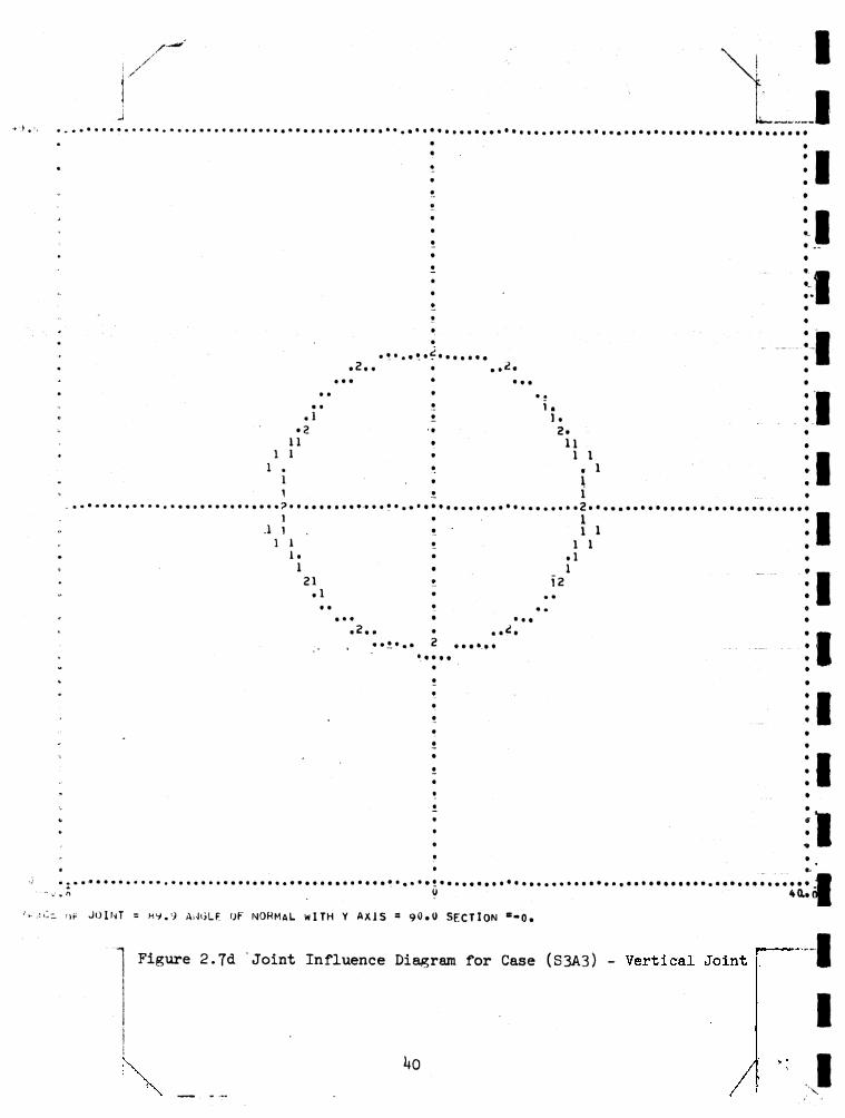
figures, "2” denotes the position of a rock bolt, while "1" denotes
a position inside the slip zone. (In cases S1A1 and L2A1, to save
computation time, bolts were included only in the region affecting
stresses in the upper half of the tunnel.) The working loads for
the bolts are the sum of the installed tension and resistance for the
rock load, whose maximum value per bolt is calculated from the height
of the biggest slip zone.
For the example cited, Table 2.1, Part 1, the use of low tensions
and wide spacings is cheapest (S1A3); however the large extent of the
slip zone is dangerous for the eight-foot bolts. Twelve-foot bolts
would be more reasonable. Table 2.1, Part 2, is for the initial
principal stresses vertically; in this instance, the eight-foot bolts
are too short unless a very close pattern is used. Table 2.1, Part 3,
is a similar computation where the tunnel is to be subjected to a 5 g
blast acceleration in the horizontal direction.
The basic idea is restated in Figure 2.12. As the bolt tension
is increased, or spacing reduced, the bolting pressure is increased
and this has the effect of reducing the rock load (curve A). Since
the rock load reduces the precompression supplied by the bolts to
12
the elastic zone, the volume of broken rock will enlarge unless
the bolting capacity is increased by an amount equal to the rock
load. The required supporting strength curve (B), the sum of
rock load and bolting pressure, displays a minimum. (The economic
minimum, however, may be situated differently.)
Prejudices concerning the style of rock bolt installations can
emerge from extensive calculations of the above sort. This, however,
is not the intention here, but rather the presentation of a particular
train of logic. Obviously, the details c m be changed and with them,
the results. The tunnel may be loaded by high or low pressures,
before or after rock bolt installations. The shape need not be
circular, the bolts need not be radial, and the design need not be
symmetric. Instead of mathematical solutions, the stress fields can\
be summed from finite element results. The criteria of failure
can represent a continuous material about the tunnel rather than
ubiquitous Joints. Only the sequence of logical steps is at issue.
The bolting scheme is pre-stressed to keep the zones of potential
rock fall from growing too large. But it must also have additional
untapped strength equal to the load of rock zones that tend to move
into the opening. Finally, the bolts must be long enough that their
anchors be well behind the slip zones.
2.7 CONCLUSION
The designer of a rock bolt reinforcement scheme has several
options. He can install ungrouted, untensioned rock anchors;
13

continuously grouted, untensioned reinforcing rods ("Perfo 'bolts");
or highly pretensioned bolts with or without protective grouting.
Prestressing tends to minimize the rock load by altering the stress
field around the gallery and by preventing rock deformations. In
the illustration presented which was based on an "elastic analysis",
significant reduction of the rock load by increasing the prestress
could not be demonstrated until the average wall pressure exerted
by the bolt pattern reached a significant percentage (about 10?) of
the initial rock stresses (Table 2 .5). This can be attained only
in certain classes of problems. A significantly lower threshold
pressure for rock load reduction by bolting is being obtained using
"nonelastic" solution methods where a degree of deformation is
tolerated. These studies are reported in the next section. It is
interesting to note that only the average rock bolt pressure and not
the length, and spacing of bolts seems to affect the extent of
reinforcement achieved (Table 2 .1+).
Ihe design approach offered here, which is an elastic analysis,
can be summarized as follows. The maximum extent of rock fall-in is
estimated. Applying the design acceleration, a total force required
for reaction c m be computed. If this is quickly applied by a rock
bolt installation, the full extent of the slip zone may not have time
to materialize, and the reinforcement system may be overdesigned. If
the function relating the slip zone volume to the bolting pattern is
determined, it is possible to balance the reinforcement scheme.
Ik
A large percentage of the cost of a rock holt surrounds the
drilling of the hole, the setting of the anchor, and tensioning
and grouting • The cost of a large bolt is therefore not much
greater than the cost of a small bolt, and it would seem the
cheapest solution to supply the full required reaction force with
a small number of large capacity bolts. However, the results of
this elastic analysis suggest that the mechanism of failure may
involve local movements that could occur between the bolts of a
coarse pattern. Thus the best design is a matter requiring geologic
and engineering analysis. The enormous differences in reinforcement
costs according to the scheme adopted demand that rational effort
be made to design the rock bolting installation.
15
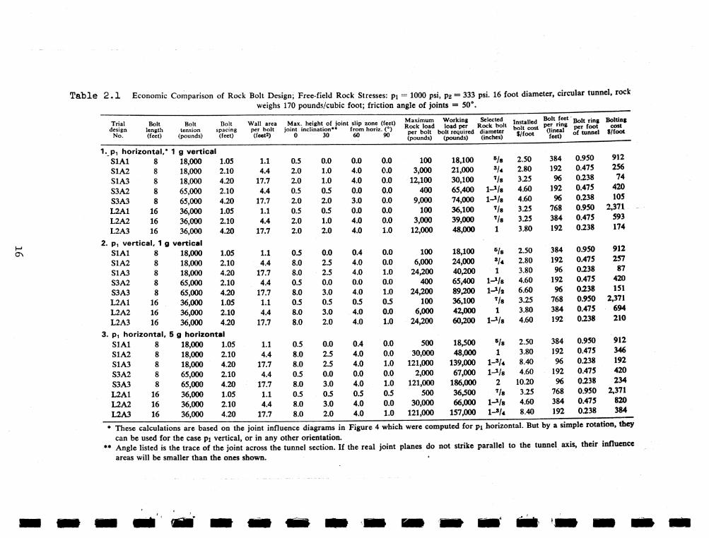
Table 2 . 1 Economic Comparison of Rock Bolt Design; Free-field Rock Stresses: pi = 1000 psi, P2 — 333 psi. 16 foot diameter, circular tunnel, rockweighs 170 pounds/cubic foot; friction angle of joints = 50°.
TrialdesignN o.
Boltlength(feet)Bolttension : (pounds)
Boltspacing(feet)
W all area per bolt (feet2)M ax. height o f joint slip zone (feet) joint inclination** from horiz. (°)0 30 60 90
M axim um R ock load per b olt (pounds)
W orking load per 1 bolt required (pounds)
Selected R ock bolt diameter (inches)
Installed b olt cost $ /fo o t
B olt feet per ring (lineal feet)
B olt ring per foo t o f tunnelB olting
cost$ /fo o t
1. Pi horizontal/ SI A l 8
1 g vertical18,000 1.05 1.1 0.5 0.0 0.0 0.0 100 18,100 DJa 2.50 384 0.950 912
S1A2 8 18,000 2.10 4.4 2.0 1.0 4.0 0.0 3,000 21,000 3U 2.80 192 0.475 256S1A3 8 18,000 4.20 17.7 2.0 1.0 4.0 0.0 12,100 30,100 Vs 3.25 96 0.238 74S3A2 8 65,000 2.10 4.4 0.5 0.5 0.0 0.0 400 65,400 1-* la 4.60 192 0.475 420S3 A3 8 65,000 4.20 17.7 2.0 2.0 3.0 0.0 9,000 74,000 U / s 4.60 96 0.238 105L2A1 16 36,000 1.05 1.1 0.5 0.5 0.0 0.0 100 36,100 Vs 3.25 768 0.950 2,371L2A2 16 36,000 2.10 4.4 2.0 1.0 4.0 0.0 3,000 39,000 Vs 3.25 384 0.475 593L2A3 16 36,000 4.20 17.7 2.0 2.0 4.0 1.0 12,000 48,000 1 3.80 192 0.238 174
2. p1 vertical, 1 g S1A1 8
vertical18,000 1.05 1.1 0.5 0.0 0.4 0.0 100 18,100 Vs 2.50 384 0.950 912
S1A2 8 18,000 2.10 4.4 8.0 2.5 4.0 0.0 6,000 24,000 V* 2.80 192 0.475 257S1A3 8 18,000 4.20 17.7 8.0 2.5 4.0 1.0 24,200 40,200 1 3.80 96 0.238 87S3A2 8 65,000 2.10 4.4 0.5 0.0 0.0 0.0 400 65,400 l-Vs 4.60 192 0.475 420S3 A3 8 65,000 4.20 17.7 8.0 3.0 4.0 1.0 24,200 89,200 l-*/a 6.60 96 0.238 151L2A1 16 36,000 1.05 1.1 0.5 0.5 0.5 0.5 100 36,100 Vs 3.25 768 0.950 2,371L2A2 16 36,000 2.10 4.4 8.0 3.0 4.0 0.0 6,000 42,000 1 3.80 384 0.475 694L2A3 16 36,000 4.20 17.7 8.0 2.0 4.0 1.0 24,200 60,200 1-V» 4.60 192 0.238 210
3. p1 horizontal,S1A1 8
5 g horizontal 18.000 1.05 1.1 0.5 0.0 0.4 0.0 500 18,500 Vs 2.50 384 0.950 912
S1A2 8 18,000 2.10 4.4 8.0 2.5 4.0 0.0 30,000 48,000 1 3.80 192 0.475 346S1A3 8 18,000 4.20 17.7 8.0 2.5 4.0 1.0 121,000 139,000 1-V* 8.40 96 0.238 192S3A2 8 65,000 2.10 4.4 0.5 0.0 0.0 0.0 2,000 67,000 l-J/8 4.60 192 0.475 420S3 A3 8 65,000 4.20 17.7 8.0 3.0 4.0 1.0 121,000 186,000 2 10.20 96 0.238 234L2A1 16 36,000 1.05 1.1 0.5 0.5 0.5 0.5 500 36,500 Vs 3.25 768 0.950 2,371L2A2 16 36,000 2.10 4.4 8.0 3.0 4.0 0.0 30,000 66,000 l-J/8 4.60 384 0.475 820L2A3 16 36,000 4.20 17.7 8.0 2.0 4.0 1.0 121,000 157,000 1-»/« 8.40 192 0.238 384
* These calculations are based on the joint influence diagrams in Figure 4 which were computed for pi horizontal. But by a simple rotation, theycan be used for the case pi vertical, or in any other orientation. .
** Angle listed is the trace of the joint across the tunnel section. If the real joint planes do not strike parallel to the tunnel axis, their in uenceareas will be smaller than the ones shown.
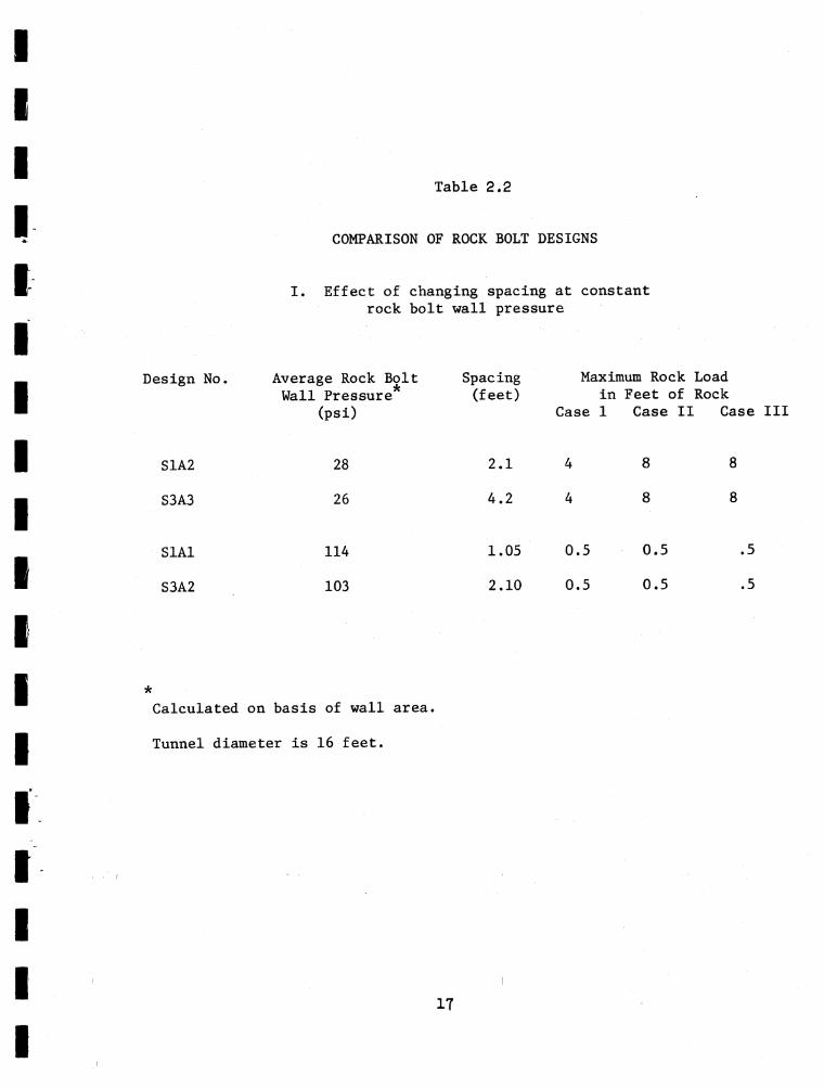
Table 2.2
COMPARISON OF ROCK BOLT DESIGNS
I. Effect of changing spacing at constant rock bolt wall pressure
Design No. Average Rock Bolt Wall Pressure
(psi)
Spacing(feet)
Maximum Rock Load in Feet of Rock
Case 1 Case II Case
S1A2 28 2.1 4 8 8
S3A3 26 4.2 4 8 8
S1A1 114 1.05 0.5 0.5 .5
S3A2 103 2.10 0.5 0.5 .5
*Calculated on basis of wall area.
Tunnel diameter is 16 feet.
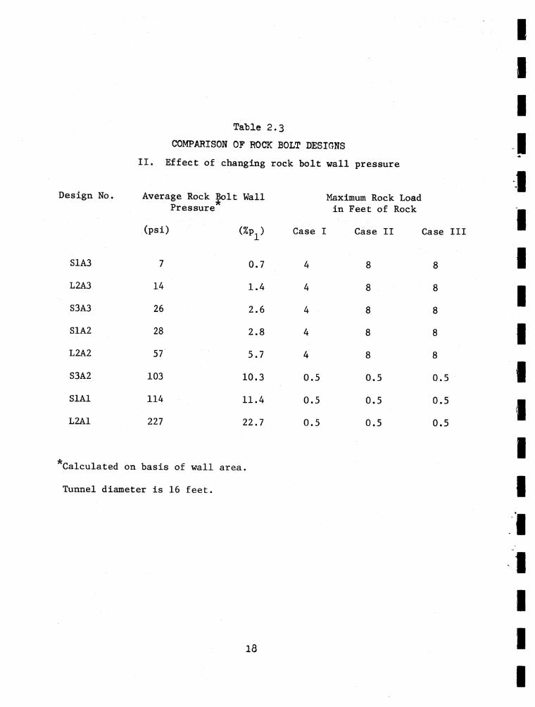
Table 2.3COMPARISON OF ROCK BOLT DESIGNS
II. Effect of changing rock bolt wall pressure
Design No. Average Rock Pressure
Bolt Wall * Maximum Rock Load in Feet of Rock
(psi) (%PX) Case I Case II Case
S1A3 7 0.7 4 8 8L2A3 14 1.4 4 8 8S3A3 26 2.6 4 8 8S1A2 28 2.8 4 8 8L2A2 57 5.7 4 8 8S3A2 103 10.3 0.5 0.5 0.5S1A1 H 4 11.4 0.5 0.5 0.5L2A1 227 22.7 0.5 0.5 0.5
*Calculated on basis of wall area.Tunnel diameter is 16 feet.
I
L O A D 10.000 POUNDS; LEN G TH 10 FEET; TENSION POSITIVE.
o-H
T
r
i
TENSION
SHEAR FAILURE
BOTH
UNSHADED REGION REPRESENTS NEITHER TENSION NOR SHEAR FAILURE
FIG.2.2 COMPARISON OF STRESSES WITH FAILURE CRITERION.
After Duncan and Goodman (1968)
*0*0
i 1 1 Jm i n } i n i u i n U n i • ¿ i
i n n .22.
n 11 ¿ 1211U ' 1 2
1 1 1 1¿121211 n n n linn
? i¿i n i n i12* i u u ?. m u
.2 • *2«
2.i n nii ii m i 11n n u ii m i
i i i u m i m u n i v iu n i i n i in n n n mi i i
.2.. i n n n. ii ii
mi n mi un i n i n n u i n n n i i i
un ni i ii inni i i i
7 r a Cl J u I f j T s
40., ANuLF OF NORMAL WITH Y a x i s = 9 0 . 0 SECT ION s ~ 0 ,
>1 A l
Figure 2.3a Joint Influence Diagram for Case (SlAl) - Horizontal Joint
21
.•¿.?U^l?i21]
• ?
11 J ?.1 1m i?!¿1n li i1111n i i u nm i uii n lii
?i*u 121l ?i i i
?A 1 12. 1?•2
* •.2
I«
Ii
Ii
I(i
I<i
I44
I• • • 4
c(4
Iaa
Iaa
IKI
I
. oT^Ce. J'vI'J!SI l
;i<M'ial v l I fi i h«:ii - gy, u AC T IO N --o#
Figure 2.3b Joint Influence Diagram for Case (SlAl) - 30° Joint
II22
.2#2• 2 -
2.• •
21 1121 ?112n
i ii nn m i i i i
2121i
2121. . • • 2
1 1 1
111] 1
1 111 min m i i
<L121¿11 21 l 1111
i 1 111n n u
• •.2
1 • « • •1
4 u. oTRACc. of J o l ' l l = >)}■ Y AA1S = yO • u S E C T I O N " - O *
S 1 a 1
40.
! Figure 2.3c Joint Influence Diagram for Case (SlAl) - 60° Joint
23
* \
<H) . U
.2.2 * • 2 m 2 • ¿•2.2...2.
2.11
1212112?1»?. ...
2.¿-?.12U
212112121
0*0
2121
2121
2211U.2
• • •..... . . . i
• • • •......
uTfíACt r'F JOINT = ^ . ‘y A,( )|J' <)K (J')Rm a L -»líH Y AXIS = SECTION =-Q •
SI Al1
1Figure 2.3d Joint Influence Diagram for Case (SlAl) - Vertical Joint
2k
i i i 1 i l1 11 i l l 1 ! I • 1 1 1I I ) ¿ i i • '• • ii i i ; 1. « lil i .2i • •
lU i i l ii 1 . 2 • 1 1 1 1 1 I l i I1.2* I l 1 1 1 1t . . l 11 1 1?. i ni
• «
. 2i l t • 2 • i 1 1
1 ! I l . l * 1 . . 1 i i1 1 1 Al 1 1 . 2 . 1 • i . ¿ * n M i l l
1 i 1 1 1 1 1 * ’l - ^ . l <r 1 . 2 . 1 . 1 X 1 1 1 1 \1 ] 1 l ‘ • 1 • !1 i 1 • 1 • 1 l i i i i l i
-*+ • • nHK Jv> i i J '
S 1 i * 2
4(- A i M j !... I A ) K ¡ . , L ; Î T H Y A U : i = 4 ^ . 0 S E C T I O N = “ 0 •
F igure 2.Ua J o in t In fluence Diagram fo r Case (S1A2) - H orizon ta l J o in t
25
x • \\
••¿»•if.2• •
• ?• •
1 1 1)•11.2*1 1A.I2. 1 1.1 1
1. 1 12 . 1 1 1 1. 11 . I l ?•
11 £ '11 I*1 11 11121 1 1.1 ! .2
2. .'.2
2 *1.1....2*11 . 1**1 *■ ..2«.1.1 i.i.i 1 1 1
. 0 4DT‘-?a L l Of- J O i ' l ! 4!>inLh Of NJK- ' AL <ITH Y AXi j , » S E C T I O N = " 0 .
Figure 2 .kb Joint Influence Diagram for Case (S1A2) - 30 Joint
26
'O . U
* 2 • •
.2
• *
»2
1*¿* 1M n i? . 1 i i i
i. i n i . i i i2 « 1 1 1Al UÌ?.11
o
ii •
11 i.1 1 i11 i ?A
1 11 1 .1 1 i ). \ . 21 i 1.1
11 . 2.1
. 2
. 2 • • «. •
-'+Ü
TNACL o f j o X f J T = f A-JOLH OF N O H ^ a l v ITH Y AXl* Ä gO.ü SEC T I O N = **0.
Si..2.
1 Figure 2.he joint Influence Diagram for Case (S1A2) - 60° Joint
4 0 . (
27
i i
l
. )I • ¿ # #
ni2 *
2.11
}¿
► 2...
40-0
ím > j 3KCTIon
Figure 2.Uà Joint Influence Diagram for Case (S1A2) - Vertical Joint
28
h r.. o
ï 1 1 1 11 1 ? I l l 1 1 1 1U 1 1 1 1 1 1 • l . l i .*■. V V . l . l 1 1 1 1 1 11 1
1 l ) 1 1 1 . ¿ . 1 1 1 Ì Í 1 1 11 1 I l 1 . . 1 A. . 1 11 1 1
I l 1 # • • • • 1 111 • • • • • 1
• • * • •• 3 • ? . .
• • • • •• • •
• • •• • •
•
, • •
• •
• • • • •• • •
? . . . ?1 • • • m • 1
11 1 • • * • • 1 111 1 1 1 . 1 w • 1 1 1
1 1 l I l 11 . ¿ . 1 1 11 U l 1 11 1 1 1 1 1 1 . 1 • 1 . 1 ? 1 . 1 , 1 . 1 X 1 1 1 1 1 1
11 1 1 1 11 1 . 1 . 1 11 1 1 l 111 1 • 1 1
J , o
T <ACL n.f- J >!■ T r
40.1 i ^ L f n Ü O W I A L w I M y Axis = VO'V StCTlON *-o9
Figure 2.5a Joint Influence Diagram for Case (S1A3) - Horizontal Joint
29
'»■ \ l . I)
• 2 • • • • •
1 . . i 1 .1 1 1 .
1 1 1 11 i 21
1 1 . 1 1 1 . 1
1 1.1 . ¿ . 1
••••••••••1• 1 1 11U f .1 1 .1 .1 11 .4 .. A. 1 1• 1. 1 1• 1 . 1 1• 1 . 1 1• 2. 1 1 1•' 1. 11• . 1 1• . 1• .• ••« •• •» • .• .• . 2• • •• . •«.
1 ^i . i . i1 A A
■9j#0
TWACt. o f JOINT = 3i:.‘ AN L.I- <)F NOHMa L WITH Y AXIS s 9^.0 SECTION *-f).
S]AJ F igure 2.5b J o in t In fluence Diagram fo r Case (S1A3) - 30 J o in t
30
h
l.<* 1M H li 11.111 1 ì « 1 11t. 1 112. 1 1 1 11 U 1
il I.I l i 11 i 21 l 11 1 •!1 1 1 1 .1
1 i 1 1 * 11 11 . ¿ . 1
- 4 ;•. o 4(1 -i-.L'. J J l '1 • f.u -, I f H r ^ À i s = V' J .U SFC r Tou - - c .
Figure 2.5c Joint Influence Diagram for Case (S1A3) - 60 Joint
31
40 . Ü
- 40.0
SI AJ] Figure 2.5<1 Joint Influence Diagram for Case (S1A3) - Vertical Joint
32
I \
» f l )) 0 j i a > 4 3 9 0 > O O '> o ® ° i ■» a » 8 a j o « * o o r I I) O 3 9 © 'J 0 0 0 9 9 0 t f © © © © 0 0 l » 0 0 0 3 13399 0 0 0 9 0 1>0 0 0 9 0 30
i i1 II 1 l l i l i l Ï
1 © 1 l l,UlUloll.Ul i
alol o l«loval o l<U I
l ll l U 1 1 I I {l 1
V I 1 1
« o
o o3 O
O *
o o
9 3 3 9 9 9 9 9 0 9 0 3 9 9 0 0 0 0 0 9 9 9 0 9 0 0 0 0 0
O
« ’
O
9
9
O
O11
1
l iO
i i
° 11
0 * 5 O 0 0 0 0 0 0 0 3 * © « 3 0 0 0 9 9 0• 0 0 0 9 0 0 0 0 9 9 0 ©O© 9 0 000* ^ 9 0 0 0 0 0 3® »0 0 0 0 0 0 0 0 0 9 3 0 0 «
3 9 O O
O 9l O il H
1 i> loi
l o l » l 9 l
lol<lo lo lo l
l lolol 1
l i l i 1 l l l
l il
— 4 O 9 O 9 O 3 3 3 9 9 o 9 9 3 O ï 'J 9 •'
- 4 0 „ 0
) o 9 9 9 0 0 0 0 3 0 0 " * 03 3 9 9 3 0 9 ‘3 9 9 0 0 9 9 0 9 9
O
> 0 0 9 0 9 0 0 9 . » 3> 0 9 9 3 9 0 9 0 0 9 0 3 0 0 9 0 0 0 0 0 0 0 9 9 0 0 0 0
4 0
T^'Cf: r)F J ' H N T
r n t 7
t r a i F Of isjfpM.M W ITH Y A X I S = 0 0 :>r» SFC .TU ÌN - - 0 ,
Figure 2.6e Joint Influence Diagram for Cane (S3A2) - Horizontal Joinj
33
1
A o 0 ® 9 : ’■■»>■» j o o o o o o o o o o o o o o o o o o n o o o o o o o o o o o o o o o o o o a o o o o o o o o o o o o o o o o o a i o o o o o o o o o o o o o o o ' o o o o o
-'♦no0 , , ,- 4 0 „ 0
'*p j >nr
» o o o o lo I® l i ® l e i s o n o ® Loieu 1 >1,1® 1 1® 1 1
i o 1
> 0 9 0 0 :> O 5 * » » 0 5 o -3 n > 0 0 0 9 0 0 0 9 0 0 0 0 0 9 0 0 9 0 0 9 0 9 0 9 9 0 0 9 0 0 0 9 0 0 9 5 o o <
1 lo1 lU 119 1
0 9 9 0 0 9 0 9 0 0 9 9 0 0 0 9 0 0
9 OO 9
lo 1lo 1
O l 9 1 o 1O 0 9 0 ®e o o o o o o
lo l, i
19 0 0 0 9 0 0 9 0 > 5 5 9 9 O O 1 > 0 9 9 9 9 9 9 -0 > 9 0 9 9 9 9 9 0 0 >9 9 0 9 9 - >9 5 9 0 ® 9 * 0 9 0 0 0 9 0 9 9 '4'ìl!■ ‘: ».» L C nf NfinMM WIrM Y ^XTS = <-?n,n SECTION =-0,
i Figure 2.6b Joint Influence Diagram for Case (S3A2) - 30° Joint
I0
1 Ioo
Io
Io0
1o0
10
9 O
10
10 *
1•»0
1e0
1©0
10
1 1III
3^
IIIIIIIIIIIIIIIrii
4 0 o 0 o o o o o o o o o o f t o a o o o o o o o o o o o o o o o o o o o o o o o o o o o o o o o o o o o o o o o o e o o o o o o o o o o o o o o
>990000
o o 0 o
O 5o o
1 o
O o 9 8 0 ' > 0 l > 0 > 0 î l ' > 0 a 0 0 î 9 0 i 0 4 « * 9 0 « 0 a 5 i > 9 9 l > ( > i » 0 |,> î 9 0 # 0 a i 0 aO l. 1
1*9 1 1 .o ' 1 1* I l 1 1, 1 i l « I. i l 1 1 -9 1o l 1 . 19 O l o l« • o o a o f
o a o o • < ioloU1 1lo 1 l l i lo il U i l
lo i 1Il 1 1
A O o ^ •> o > o ft n i f- 4 0 „ o
9 0 9 0 0 0 9 0999000* : >00 09 0 9 O 0 9 0 0 0 0 9 O 0 0 0 0 0 0 0 0 9 0 0 0 9 0 9 9 ao > 0 0 9 0 0 0 0 » 9 0 0 9 0 «
•yo^r.fi MF JHTM‘T = ' / » n , n fïGI T; n F T»RMM_ WITH Y AXIf' = ‘ QoO SECTION = - 0 «c v ?
L»—» Ó O O O O O O O O
> 0 0 0 9 0 9 0 > 0 0 0 0 0 0 0 0 040
Figure 2 .6c • J o in t In flu en ce Diagram fo r Case S3A2) - 60° J o in t
35
o » 8 0 0 ' ) ' ) 0 9 ' ) í ( » n o * o j ‘» 0 9 J o > o « i> * ' > « # o # o o ( » 9 ' > 9 ' » o o e * » n * * o « # #
o ®
O *
8 9 4 1 0 9 0 O O • O • O «
9 O O «
9 9 0
9 9
• O
«1 9 1
11 1
1 9
lolo111
0
1 . i1 9 1
9 0 3 9 0 9 9 0 0 0 0 9 0 0 0 0 0 0 0 0 *>0 0 9 0 0 0 0 9 9 0 0 0 0 1 ) 9 0 0 0 0 0 0 0 9 0 9 9 9 9 9 9 0 « 0 0 0 9 « 1 ^
i . 1i • I1 • o ilo o • i1 o 111 o 11
o 1 • OO
9 9 O 9 O
• 9 O
9 9 9 1
0 0 9 0 9 9
0 0 9
0 9 0 0
> O 9
O
9
O
9
O
9
9
O
^Oí n 03 »39300 9 93 9 9130 0 90 '> 9.1 000090.1 00«>0000»000900«00©0©00000900090000000000 9 000009100000000090000
-40*0 o
t r a c F O F J O I N T = 00, 9 A N G l . F n p N O R M A L W I T H Y A X I S = 9O „0 S E C T I O N = r * n .
rv?Figure 2.6d Joint Influence Diagram for Case (S3A2) - Vertical Joint
36
**.••••*•*•¿4»* * • • * • • » * » * • » . * » 4 1 * 4 * «kiil i it
i S l l U r y r r n ï r v a . v u
I r l i i i f*ii ì V n i i . i
i \ il . .
kk»2
kk
*VÒ.'Ò
m • • 4 k • • • • • • • • • kI » • • k k k • k • k k • 2 Vk k k k k • • k k • • • k k k • k k
» i m i l . r . i 1- i ï Si. i . J^ ■ ¡ w -
l w L 11 \ S ii
k k .............................2k
kkk2.
ÌÌ \ Y. lÌ \ 1 Yì
^ \ 11 ^ \ n \ n S . i ; \ ? i ’.v.yiï i ; ï 1\ \ 1 1 U V .i-.l it 1 1 V W
k
• k • « k k k • k k' kk • k • k k k k 2 k k • • • k k k k k k k k k k k k k ’k k • k k k '1« k
• •
k• 2
i 1 «iv. i i L ï L
ïwfe> li il i Y 1
iè
_ . i k %
■ J•
__kkki%ï
__ 3iÌ
11'I1Ì
. T 1 \ 1
rVkkl1111
_ 1 1
i
'*6
TRÀCES Va')
n‘r Joint s f(. ang'l'e or norNa'l witn v axis » $o»o section *h-ô.
I
J o in t In flu en ce Diagram fo r Case S3A3) - H o rizo n ta l J o in t
37
«*
40,0
.2..• • •..l.*
• 2
1 1 H.lM.l 11.11. 11.1 1 _ 1. 1 1 2. 1 1 1 1. U . 1 1
V
<►0.0
11.11 1.1 1 1
11 1 21 1 1.1 1 .1.2• .
1.1.2.11 • 1 i 1 • 1 i* ......U 1.1.1ill
. • 2 •
•<►0TRACE. OF JOINT = 3 a. o AN Lfc OF NORMAL WITH Y AXIS 3 90.0 SECTION *-()•S3A 3
Figure 2.Jb Joint Influence Diagram for Case (S3A3) - 30° Joint
40
1/ V
40.0
.2..• • •
• • • •.2
l.¿» 1l .U Ï 11
ï . 1 1 1 1 i-, 1 11.1. 1 1 ï2. 1 1 1
11 11 1• '11
11111 1.
1 1 1 11 121 1 11 1 .1
1 1 1 1 .1 1 11.1 1 11 .2.1
• 2
• • • » • •
- 4 0 • o ü
r ■ ■ ' ITRACI: or JOINT s feo.M AMOLE OK NORMAL WITH Y AXIS = 90.0 SECTlpN s-0.S 3 A 3
40
Figure 2.7c Joint Influence Diagram for Case (S3A3) - 60 Joint
39
•• ìC- r,f JOINT = M9.9 ANGLE OF NORMAL WITH Y AXIS = 90.0 SECTION “-0.
Figure 2.7d Joint Influence Diagram for Case (S3A3)
1»0

IIIIIIIIIIIIII
1uni i1 11 1 121? l \ 11 •?!
• 22 .
# •
112121122121211?121
1*.
11 11111
1 11 1 11 U2 .
2.
2.2
2*2
?2 .
? •* 2 .
11 1
i mii l i
l in
.?121
121 1 1121
2 ..2
.2
211212 .2 21 211? 11111
1 1m i l
l l i m l
ì
40
III
I ,, r {- Dr j » i ' T = <) . J aN'-U . OK hOPMAL WtTh Y AXIS = 9 0 . 0 SECTION s - 0 00
: J I !
Figure 2 .8 a Jo in t Influence Diagram fo r Case (L2A1) - H orizontal Jo in t
Ul
2•2.2
• 22
. . 2 . 2 1 1 2 2 1 H 1 2 U2.2 2121
1*1211?U
212
2 ?•2*22
2121?1 2 l 1?
1211211, 211212 2
11 111
..22 . 2,.2
22.
.22.
0] ' " T = *r"lt OF NORMAL w tTk Y AXIS = 90.0 StCUON =-() • 00
"Figure 2.8b Joint Influence Diagram for Case (L2A1) - 30° Joint
k2
II H(> . 0
I• • ? • 2 •.2.? ¿•2.2..
.22.. *5
.2
2121 1¿1
211?U
21 21 1?121
» 0.0
2121
22."5 l 2 1 .2*21?
121 1211
. 2♦2• *2 .2.2..?-
2.
oI ^ATF OK JO INT = i i . i a :*.-i.K OK I OPMAL WTT>- Y A X I S = 9 0 . 0 S EC T I O N = - 0»00
• i
40
Figure 2.8c Joint Influence Diagram for Case (L2A1) - 60° Joint
I ' U O
li . o
• ¿ • 2 • 22.2.2..,2.?• 2 •.2i 1 1?1?1)?21.2 .... .
?121r>\2 i.2
• 2 «.2 ..2 • • 2 • 2
?.2,.2 .2.1?1 1 21
■2i Î?121....2.
? 21 11 22 •.2.
• *2.2.2. •?
fPArt- Oh j u p I = ' < i . v Af (, t f. OK KOHhAL Y a XTS = 4 0 * 0 S t C H O N a " 0 #00
^ A I
1
40.0
Figure 2.8d Joint Influence Diagram for Case (L2A1) - Vertical Joint
1+4
/*
u.0. 0
V 0 . ( J
1 1 1 1 . 11 1 11 1 1 1 1 1 1 1 . 2 . 1 1 . 2 . 1 1 . 2 . 1 1 1 1 1 1 1 1 1
1 1 1 1 1 1 . 2 . 1 1 . 2 . 1 1 1 1 1 11 1 1 . 1 1 . 1 1 1
11 1 . 2 2 . 1 1 1• • • •
• . • • •. 2 2 .
• • • ••• • •
. 2 • 2 .• •• • m
• •, • • •
2 • 2. • • ••
• • .2 . • . 2
• • • • •11 1 . 2 • 2 . 1 1 1
l 1 1 . 1 • 1 . • 1 1l 1 1 11 1 . 2 . 1 1 . 2 . l 1 1 1 1 1
1 1 H I 1 1 . 1 . 2 . 1 2 1 . 2 . 1 . 1 1 1 1 1 1 l 11 1 1 11 1 . 1 . 1 1 1 1 n
II
- C • 0 0i I mU l F JOINT = 0.0 ANOLI OF NORMAL WITH Y AXIS = 90.0 SECTION =-0.00
l, a;;
4 0,
Figure 2.9a Joint Influence Diagram for Case (L2A2) - Horizontal Join
^5
vO.U
»2. • 11
.2
1 1 11 »11 • 2 • 1 1 .2.1.1
1. 1 1 1. i 1 2.1 1 i 1. 11 •
2 .
*0.0
211 1 .1 1 1 11 1 21
1 1 .1.2 2 .1.1
. 2 . 1 . . 2 .. 1.2 . 1 2 . . 2 ...11 1 .1.1l 1
-4 0 40*T K / C t : UF JOINT = 3 0 . 0 ANGLF OF NORMAL WITH Y AXIS = 9 0 . 0 SECTION =-0 .0 0
L 2 A 2Figure 2.9b Joint Influence Diagram for Case (L2A2) - 30° Joint
/
0.0
III1II1IIIIII-4Q.0
.2
• 211»2 • «
1.2.1 . 1 1 1 1 2. 1 1 1 1
1 . 1 11 1 . 1 1 1 2. lii
11 1 12.11
II1I
1121 l.I l l
11 1 21 1 11 l .1
1 1 1 1 .2 1 11.1 1 . 2.1
. . . 2..
.2
2 .». 2 . ..
-40.0 0IKACl CF JO INI = 60.0 /NOLfc OF NORMAL WITH Y AXIS = 90.0 SFCTI ON =-0 .00
L2A2
40.0
Figure 2.9c Joint Influence Diagram for Case (L2A2) - 60° Joint
1*7
I 2k 2Figure 2.9d Joint Influence Diagram for Case (L2A2)
U8
t 0.0i
‘1IIIIi(11IIk
I
i l l . l li i n l l i i l l.i.ii, 11 1 1 1 1 .2.1
1 1 11 1 . . 1 Il 1
l
111 1 1 1 1
. 1 1 . 1 . 1 1 1 1 1 1 l ì 11.2. 1 1 1 1 1 1
1 . . 1 11 1 1 . . 1 11,
.. 12 . ........
V
.0
2 .1 . . . . . 1
11 1 . . . 1 11 1 1 1 1.1 . ! . . 1 1 1 1 1 1 11 11 .2. 1 . 1.2. 11 11 1 1 1
1 1 1 111 l 1 . 1 . 1 . 1 2 1 . 1 . 1 . 1 1 I l i 1 1 111 l 1 Î 11 1 . 1 . 1 l i T 1 1 11
l . 1
■ I - 4 C . Ü 0
^..VkACL CF JOINT = 0 . 0 ANGL* OF NORMAL WITH V AXIS = 9 0 . 0 SLCT ION = - 0 . 00i L"s-..4 0 . 0
1
Figure 2 .10a Jo in t Influence Diagram fo r Case (L2A3)-H orizontal Jo in t
1*9
, 1. 21 1 11
, 11 .1 .11 1.?.
1.11. 1
1. 1 1 1 . 1 1
2. 1 1 1 1. 11 . 1 l
III
; 0 . J
t 1 .11 1.
1 1 1 11 121
i 1 . 1 1 .1
• 2
1.1.2.1
1.1.1. 1 2 • 11 1.1.1
1 1 1
. . 2 .
(
III1
— 0.0 0
i I o c OF Jiilfv'l - V>.0 / H( |_ OF UmPOIAI with Y AXIS = 90.0 SI C7 l LN = -0 .00
L ,F i g u r e 2 .1 0 b J o i n t I n f l u e n c e Diagram f o r Case (L2A3) - 30 ° J o i n t
40
50
X
III1I1IIIIIt
1 . 2 . 1 1 . 1 1 1 11 1.111 1 1.1 11 1.1 11
? . 1 l 1 11 11 l1l...?.
111111.1 1 1 U 1 21 l 1.1 1 .1
1 1 1 1 . 11 1 l.l1 11 . 2 . 1
.2
. 2 .
f jf U r 1 i f]<.i , it m t h v vx t sr ( i I r r ~ - 1). oo
Figure 2.10c Jqint Influence Diagram fop Case (L2A3) - 60° Joint
'.0
51
.3
.1.2
11 l 1
1 .11
. .2 ........1
I 1 1 1 l i.
121
.1
.2
I'
I
22.
1.1«2 • .....11 11 1•11
1
11 l
1 1 • 11
12
• • 22
I1I11II
'j. Ü ojnira = s j ur- normal with y axis = 90.o sfction =-o, oo
I• -
I4 GI
Figure 2 .10d Jo in t Influence Diagram fo r Case (L2A3) - V e rtic a l Jo in t 1II52
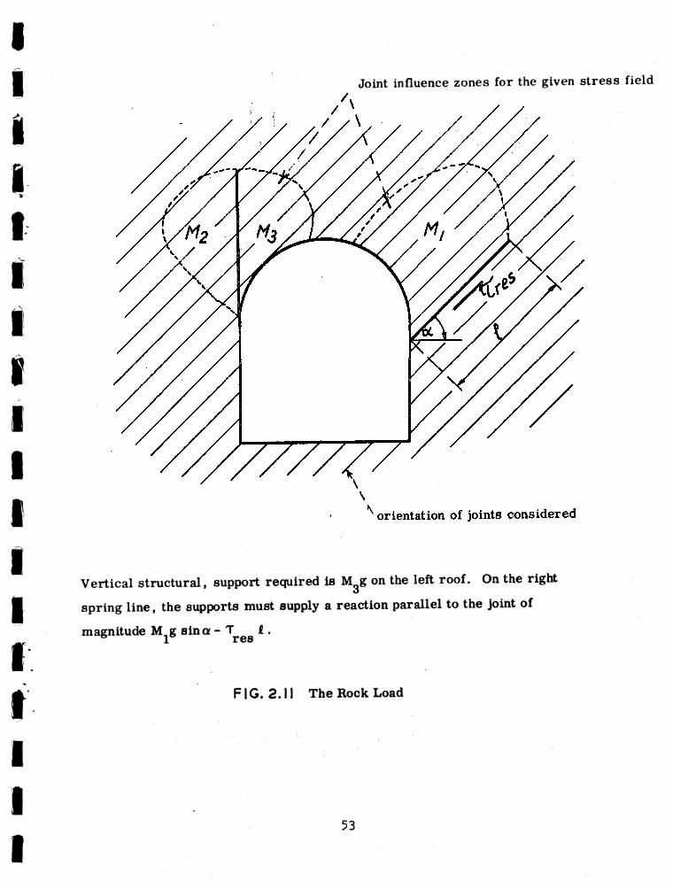
Joint influence zones for the given stress field
Vertical structural, support required is Mgg on the left roof. On the right spring line, the supports must supply a reaction parallel to the joint of magnitude M^g sin a - £ .
FIG. 2.11 The Rock Load
53
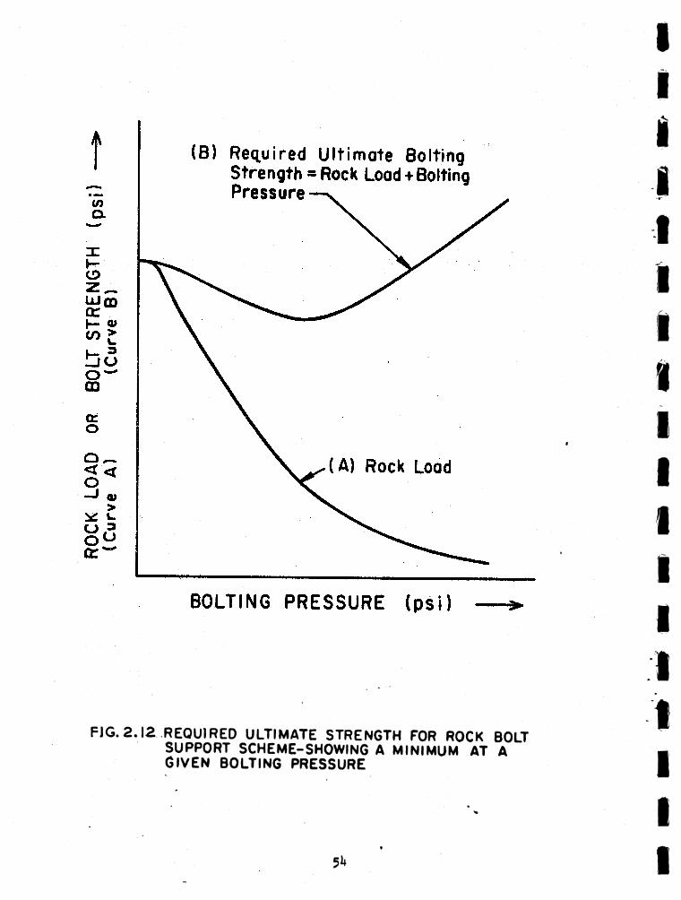
FIG. 2.12 REQUIRED ULTIMATE STRENGTH FOR ROCK BOLT SUPPORT SCHEME-SHOWING A MINIMUM AT A GIVEN BOLTING PRESSURE
5k
CHAPTER 3
IIIIII8II8KIIIIIII
DESIGN APPROACH FOR ELASTIC-PLASTIC ROCK UNDER HYDROSTATIC LOADING
Chapter 2 considered an approach to selection of rock bolt
design parameters. A specific illustration of the suggested
approach to examine the relative influences of bolt length,
spacing, prestress, and diameter made use of elastic stress
distributions assuming the rock bolts to be colinear point loads
in a linearly elastic medium. Joints were considered as a
criterion of failure, but Joint failures were not allowed to modify
the global stresses.
For simple stress states it is possible to obtain an elastic-
plastic type of solution in which the failure of specific portions
of the rock around the tunnel changes the conditions of the problem.
This chapter will draw on the logical steps of Chapter 2 to obtain
a closed form solution for design of rock bolt support of a circular
tunnel in broken rock under a hydrostatic state of stress. The
rock bolts are replaced by an average bolting pressure Pg.
13.1 MATHEMATICAL CONDITIONS
Excavation of the cavity and external loading are considered
to develop a stress state that is plastic near the opening and
elastic beyond as in Figure 3.1. The stresses in the plastic
1 Ref. 3
55
zone are constrained by the Coulomb strength characteristics of
the broken material Cr and <|>r (Figure 3.2), which may be
approximated by the residual strength parameters deduced from
direct shear tests carried to large deformation. The dimensions
of the plastic zone are fixed, on the other hand, by the criterion
of failure applicable to the rock mass at the limit of strength
and therefore by Cp and $p, the peak strength values determined
by triaxial or direct shear test. In a continuous rock mass,
or one with initially tightly closed or incipient extension joints,
Cp and <|>p are essentially the peak strength parameters for rock
substance and greatly exceed Cr and <(>r . In an open, jointed rock,
or one with shear joints, the values of Cp and <|>p may be close to
Cr and <j>r (Reference *0. See Figure 3.3.
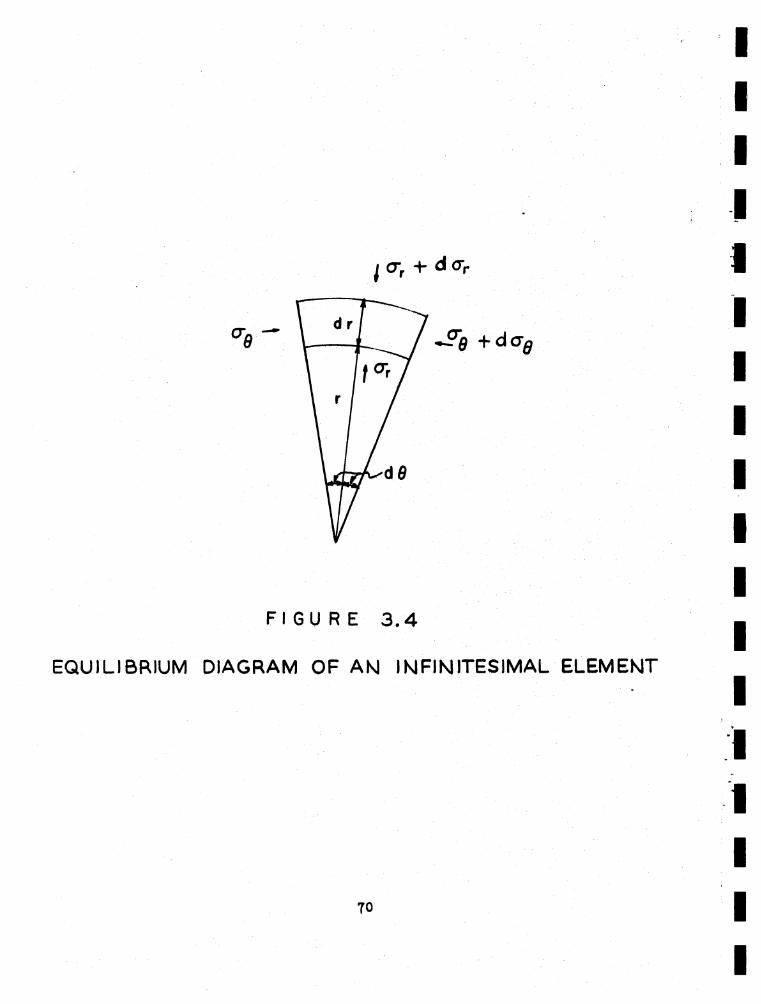
equilibrium equation (Figure 3.^)
do.
dr
0 - 0r 0 s o (3-1)
stress relationships in the plastic zone
°n + C cot 1 + sin <f>' ' 3 ? 1 * -M----- ---------- = --------- - (3-2)
o + C cot <f> 1 - sin <f>r r r r
in the elastic zone:
as r -*■ °°, a -► p, the hydrostatic external pressure or initial
stress condition. The stresses are
56
(3-3)
°0 = p * -2rwhere:
K is to be determined by the boundary conditions
3.2 SOLUTION FOR STRESSES AND EXTENT OF PLASTIC ZONE
Equation (3-2) may be solved to express o Q explicitly in terms of ar, which may then be substituted in equation (3-1). This yields
dodr
r arr
2 sin <|>r Cr cot <f>r 2 sin $l-sin 6 r 1-sin d>
1 r(3-fc)
orda
+ Crr_____cot <J>r)
dr 2 sin 6 __________ rrr (l - sin <f> ) rr
giving
°r + Cv cot * =r r rIf Rq = the radius of
boundary condition atto a pressure Pg is
2 sin <f>r1-sin <{>„ (3-5)D (r) r ^
the tunnel and D is a constant, then the
the wall of the tunnel (r = Rc) rock bolted
PB ‘
57
from (3-5)
+ Cr cot <j>r2 sin <t>r
1-sin <J>r
so that
or = - Cr cot <|>r + (PB + Cr cot <|>r) 12 sin-sin 4 ( 3-6a)
while substituting (3-6a) in (3-2) yields2 sin <j>_1+sin 4>r --------
a0 =-Cr cot d»r + - - - - - (PB + Cr cot 4r) / M l - s i n <j>rr \R°/ (3-6b)
At the elasto plastic boundary r = R and
(ar ) elastic plastic
givingK_
p - R2 = - c cot <J> + (PB + Cr cot 4>r) (02 sin 4j 1-sin 4,
(3-7)
The rock is at its peak stress at the elastic plastic boundary
so that the elastic stresses satisfy the criterion of failure
(Equation 3-2), when the peak values of $ and Cp are used for 4r and Cr respectively.
K_P + R2 + C_ cot 4 _________ _P______£
K_p “ R2 + Cp cot 4p
1 + sin P1 - sin éP
(3-8)
Equation (3-8) can be written
Kr2” = (p + Cp cot <(>p ) sin <f>p (3-9)
which can then be substituted in Equation (3-7) and solved to
give an expression for the thickness of the plastic zone.
p + Cr cot <|>r - (p + Cp cot <j>p ) sin <|>p
PB + Cr cot *r
1-sin <l>r 2 sin <t>r
(3-10*)The formulas (3-6a) and (3-6b) define the stress state in the
plastic zone, while (3-3) with K and R as given in (3-9) and (3-10)
specify the stresses in the elastic zone. However, the primary
object of the derivation is Equation (3-10) which gives the extent
of the plastic zone, and consequently the upper bound of the rock
load under gravity (for a given acceleration). (Compare with
Figure 2.12). It is seen that the rock load vs. bolting pressure
relationship depends on the external rock pressure p and the bolting
pressure PB as well as the peak and residual strength parameters.
In reality, the <|>r and Cr values should vary from truly residual
properties near the tunnel wall where large deformations can occur
to larger values not much different from the peak at points near
the elastic plastic boundary where deformations must be more
restricted.
* If <{>r = <f>p and Cr = C^, (3-10) reduces to the formula given by T. A. Lang in Ref. 3.
59
For computations herein a single (average) set of values Cr
and <j>r was adopted to characterize the entire plastic zone. The
weight of rock in the plastic zone above the tunnel is
y (R - R0 )(2R0 ). This is an upper bound to the vertical rock
load (under gravity acceleration only). (R - R ) also sets the
minimum acceptable length of rock bolts if they are installed
radially. To allow for anchor slip and to provide a margin of
safety the rock bolts should be at least (U/3) (R - RQ ) long.
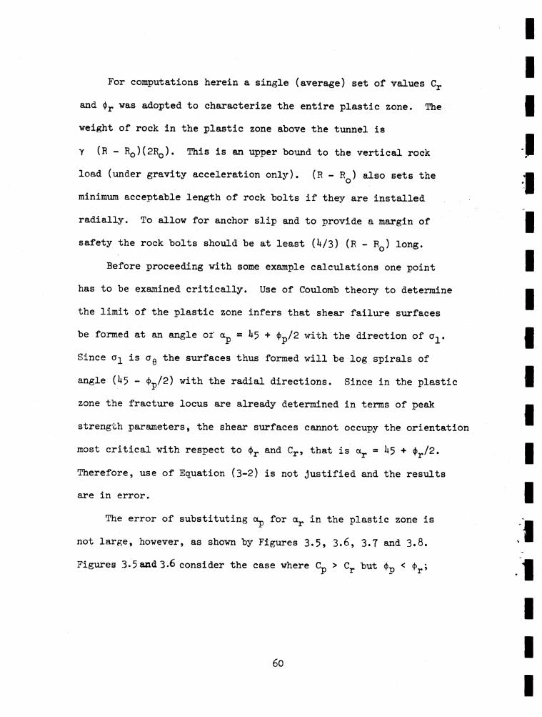
Before proceeding with some example calculations one point
has to be examined critically. Use of Coulomb theory to determine
the limit of the plastic zone infers that shear failure surfaces
be formed at an angle of otp = 1*5 + <j>p/2 with the direction of o- .
Since o-L is a0 the surfaces thus formed will be log spirals of
angle (1*5 - 4>p/2) with the radial directions. Since in the plastic
zone the fracture locus are already determined in terms of peak
strength parameters, the shear surfaces cannot occupy the orientation
most critical with respect to <}>r and Cr , that is a r = 1+5 + <|>r/2.
Therefore, use of Equation (3-2) is not justified and the results
are in error.
The error of substituting Op for a r in the plastic zone is
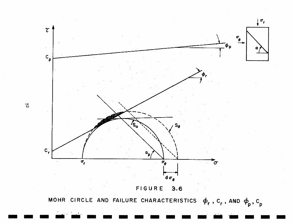
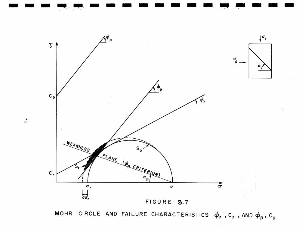
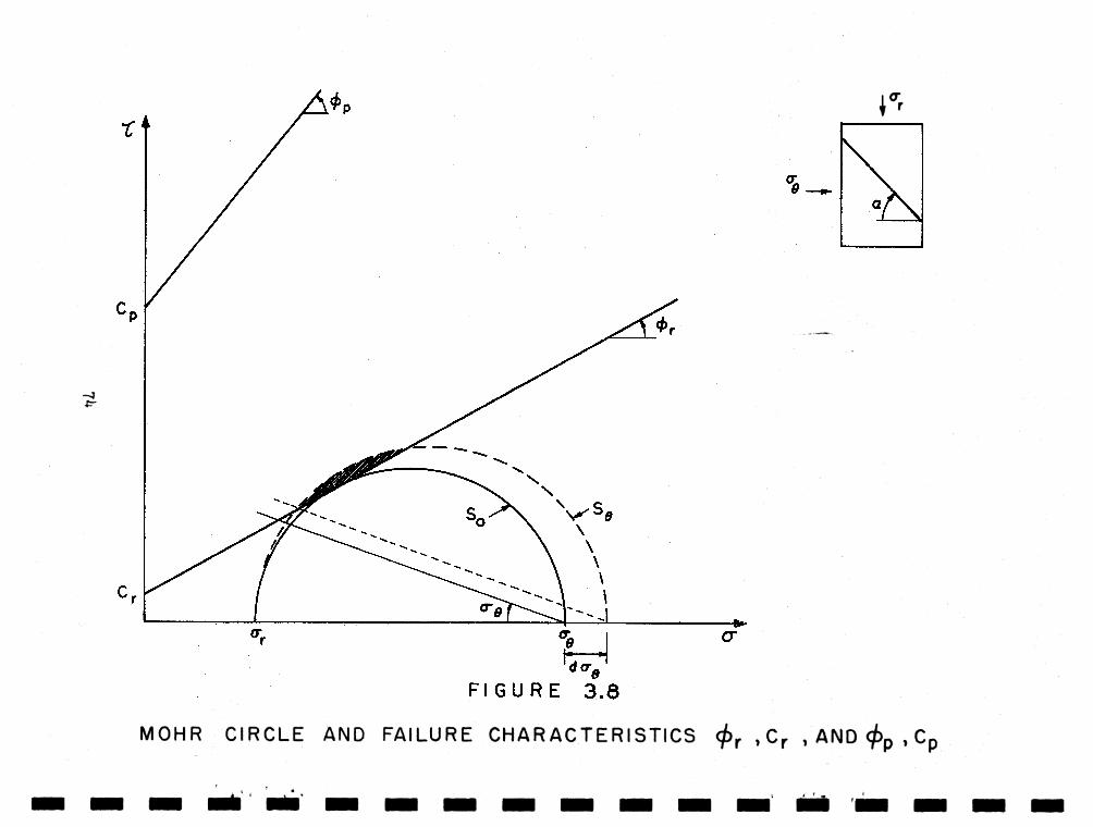
not large, however, as shown by Figures 3.5, 3.6, 3.7 and 3.8.
Figures 3.5 and 3.6 consider the case where C_ > C but 4>_. < <(> ;Jr ■* ir A
60
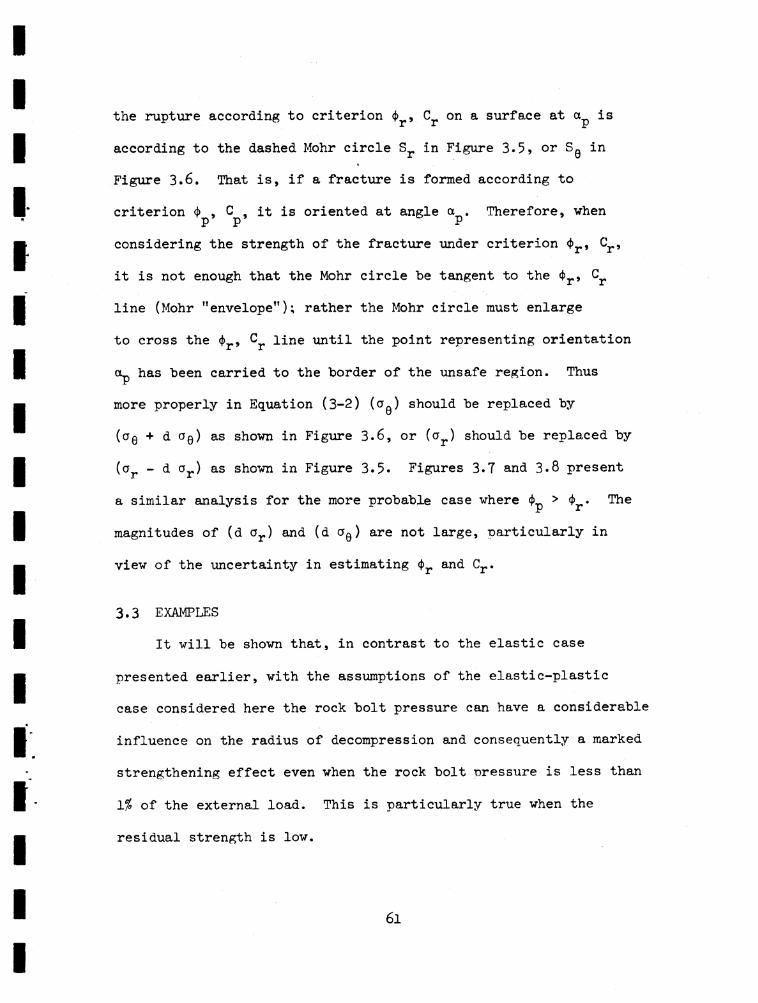
the rupture according to criterion <j>r , Cr on a surface at is
according to the dashed Mohr circle Sr in Figure 3.5, or SQ in
Figure 3.6. That is, if a fracture is formed according to
criterion 6 , C , it is oriented at angle a . Therefore, when p* p ’ e Pconsidering the strength of the fracture under criterion <t>r , Cr,
it is not enough that the Mohr circle be tangent to the 4>r , Cr
line (Mohr "envelope"); rather the Mohr circle must enlarge
to cross the <f>r, Cr line until the point representing orientation
otp has been carried to the border of the unsafe region. Thus
more properly in Equation (3-2) (Oq ) should be replaced by
(o q + d 0q ) as shown in Figure 3.6, or (ar ) should be replaced by
(or - d or) as shown in Figure 3.5. Figures 3.7 and 3.8 present
a similar analysis for the more probable case where <i>p > <f>r . The
magnitudes of (d ar) and (d a0) are not large, particularly in
view of the uncertainty in estimating <(>r and Cr .
3.3 EXAMPLES
It will be shown that, in contrast to the elastic case
presented earlier, with the assumptions of the elastic-plastic
case considered here the rock bolt pressure can have a considerable
influence on the radius of decompression and consequently a marked
strengthening effect even when the rock bolt pressure is less than
1% of the external load. This is particularly true when the
residual strength is low.
6l
Several examples have been calculated with characteristics
of the elastic material as follows: CL = 380 psi; <f> = 60°.P PFor the broken material the friction angle (<|>r ) was either
50° or 30° while the cohesion Cr was either 2 psi or 0. An
external hydrostatic pressure of 2000 psi or of 3000 psi was assumed.
The radius of the decompressed zone was calculated corresponding
to varying rock bolt pressures. For each set of properties the
curve relating bolting pressure and rock load (compare with Figure
2.12 of Chapter 2) could be sketched as presented in Figures
3.9 to 3.12. Several values of R/Rq corresponding to an external
pressure of 2000 psi are given in Table 3.1.
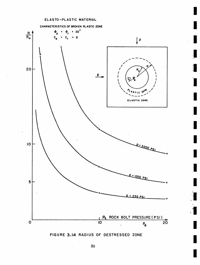
Figures 3.13 and 3.1^ show another case, — this one for a
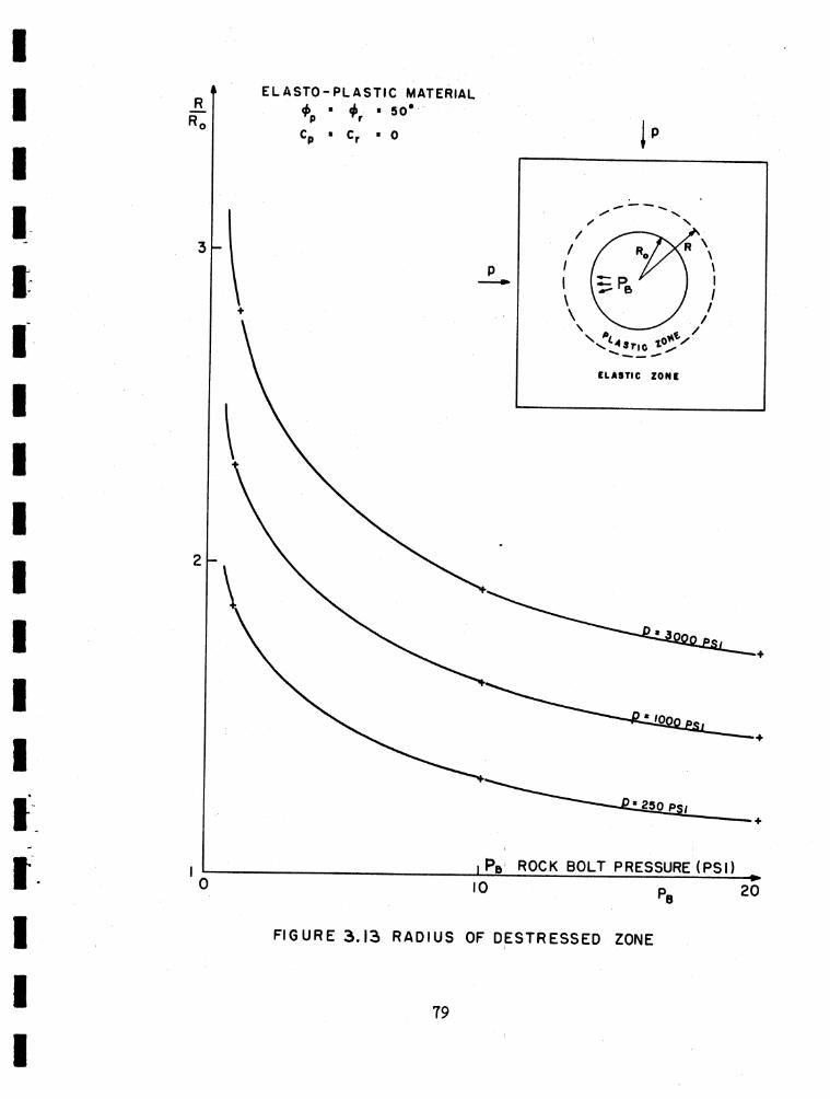
granular soil-like material in which <L, = <b and C = C . Here1 P P rthe rock bolt pressure is all that preserves the structure from
collapse. Figure 3.13 corresponds to <j> = 50°, while Figure 3.11*
corresponds to <j> = 30°. The rock load - vs. bolting pressure
functions are sketched for hydrostatic pressures of 3000, 1000,
and 250 psi.
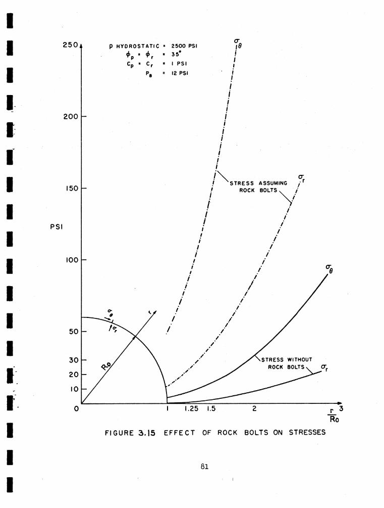
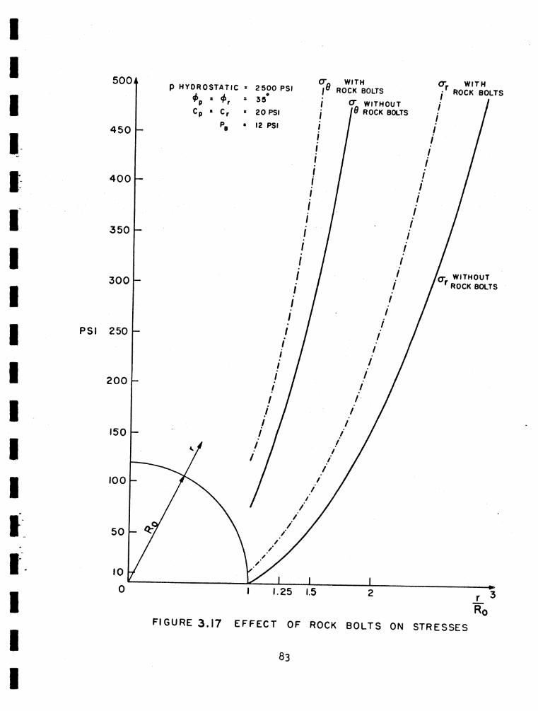
Figures 3.15 to 3.18 compare the radial and tangential stresses
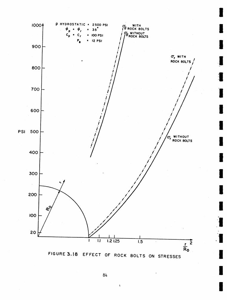
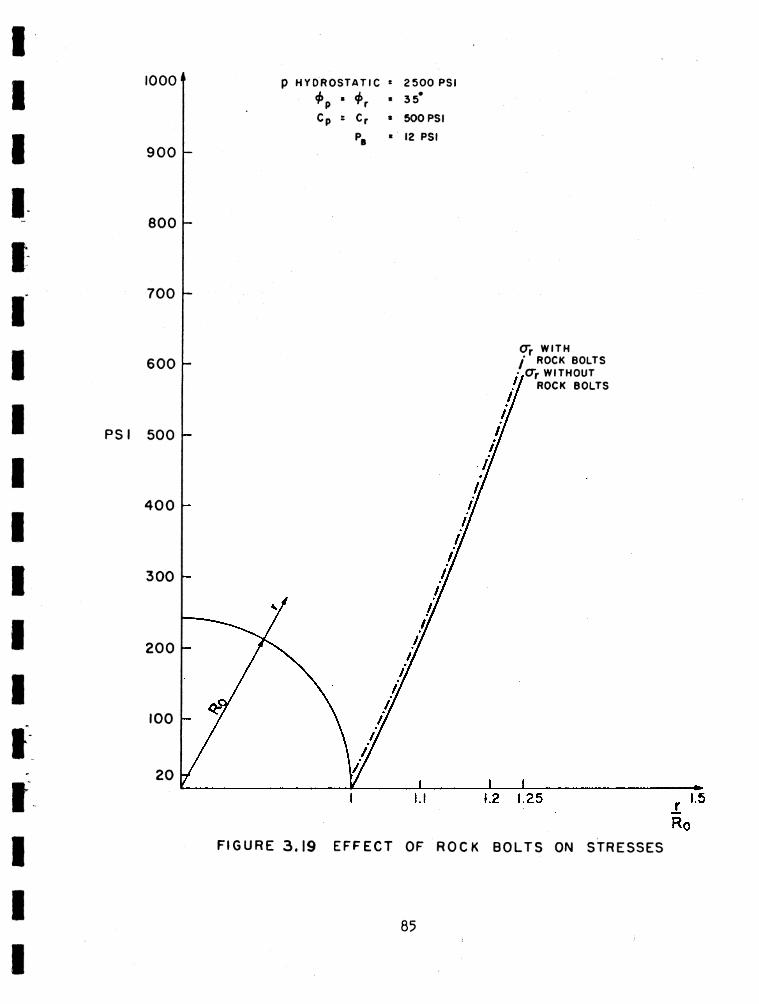
before and after rock bolting. The external hydrostatic pressure
is 2500 psi and the rock bolt pressure is 12 psi. <t>r = <j> = 35°;PCr = Cp : = 1 psi (Figure 3.15), = 5 psi (Figure 3.16), = 20 psi
62
(Figure 3.17), = 100 psi (Figure 3.18), and = 500 psi (Figure 3.19).
It is evident that the greatest relative strengthening effect
occurs when the rock is weakest. The variation R/R with C is aso
presented in Table 3.2. Design of the bolting parameters follow
from knowledge of the R/RQ vs P- relationship; as described in
Chapter 1. Two examples follow.
3.3.1 Example Ho. 1 — A 20 foot diameter tunnel (R0 =10')
is subjected to a hydrostatic residual stress of 2000 psi, and
the properties correspond to Figure 3.12 with <J>p = 60°, C = 380 psi,
<J>r = 30°, and Cr = 0. The rock weighs 1 psi per foot, and the
weight of rock to be supported is given by R/R0 . Results of the
analysis are given in Table 3.3. Since the bolts are shortest
in case 3, the economic minimum may be closer to case 3 than to
case 2. Finally, selecting a spacing of bolt; the required
size of bolt is established. If the bolt spacing is 3 feet with
total bolt pressure of 30 psi, the bolt pretension load is 39,000 lbs.
n bolt pretension load (pounds)30 = 3 x 3 x ik\ sq. in.
Pretension 7/8" bolts to 50$ of yield load to install the required
bolt pressure.' ! ' . I
3.3.2 Example No. 2 — A 20 foot diameter tunnel is subjected
to a hydrostatic pressure of 2500 psi, and the plastic zone
i
63
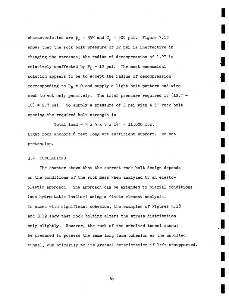
characteristics are 4>r = 35° and Cy = 500 psi. Figure 3.19
shows that the rock bolt pressure of 12 psi is ineffective in
changing the stresses; the radius of decompression of 1.27 is
relatively unaffected by PB = 1 2 psi. The most economical
solution appears to be to accept the radius of decompression
corresponding to PB = 0 and supply a light bolt pattern and wire
mesh to act only passively. The total pressure required is (12.7 -
10) = 2.7 psi. To supply a pressure of 3 psi with a 5 ’ rock bolt
spacing the required bolt strength is
Total load = 3 x 5 x 5 x l U « 11,000 lbs.
Light rock anchors 6 feet long are sufficient support. Do not
pretension.
3.H CONCLUSIONS
The chapter shows that the correct rock bolt design depends
on the conditions of the rock mass when analyzed by an elasto-
plastic approach. The approach can be extended to biaxial conditions
(non-hydrostatic loading) using a finite element analysis.
In cases with significant cohesion, the examples of Figures 3.18
and 3.19 show that rock bolting alters the stress distribution
only slightly. However, the rock of the unbolted tunnel cannot
be presumed to possess the same long term cohesion as the unbolted
tunnel, due primarily to its gradual deterioration if left unsupported.
6b
This vital aspect of rock bolt strengthening is not evaluated by
the preceding methods.
6 5
TABLE 3.1RADIUS OF PLASTIC ZONE FOR VARIOUS ROCK PROPERTIES
Figure Elastic ZoneCP(pii)
Plastic Zone
Cr(psi)
Rock Bolt Pressure (psi)
R/B0
3 .9 60° 380 50 2 1 1.66f t »1 I t f t 10 1 .3 3
3.10 f t f t 50 0 1 I .9 2f t f t f f f t 10 1.36
3.11 f f f t 30 2 1 1*.17t l f t f t I f 10 2 .1 a
3.12 f t f t 30 0 1 8.57f t f t f f f f 10 2 .7 3
TABLE 3.2VARIATION OF THE PLASTIC ZONE WITH C
C (psi) 1 5 20 100 500
R/Rq 5.02 k.kl 3.35 2.08 1.26
TABLE 3.3
EXAMPLE NO. 1 RESULTS
Rock bolt pressure P^ psi R/R0 Rock Load
psiRequired total bolt pressure
(1) 5 k.2 32 37
(2) 10 2.9 19 29
(3) 20 I.9U 9.U 30
(U) 30 I .58 5.8 36
66

r
F I G U R E 3.1
PLASTIC AND ELASTI C ZONES
67
F I G U R E 3 . 2
P L A S T I C STRESS CRITERION
68
SHEAR DISPLACEMENT
Peak a n d r e s i d 'Oa l s t r e n g t h s
69
F I GURE 3 . 4
EQUILIBRIUM DIAGRAM OF AN INFINITESIMAL ELEMENT
T O

MOHR CIRCLE AND FAILURE CHARACTERISTICS <j>r , Cf , AND <jbp , C
MOHR CIRCLE AND FAILURE CHARACTERISTICS d> ,C . AND db C* r ' r p » p
X t
- '« JU>
MOHR CIRCLE AND FAILURE CHARACTERISTICS <£r , Cr , AND <pp , Cp
MOHR CIRCLE AND FAILURE CHARACTERISTICS <£r , C r , AND <£p , Cp
75
FIGURE 3.10 RADIUS OF DESTRESSED ZONE
76
Ip
FIGURE 3.11 RADIUS OF DESTRESSED ZONE
77
78
________________________ i Pb ROCK BOLT PRESSURE (PSI)IO pB 20
FIGURE 3.13 RADIUS OF DESTRESSED ZONE
79
ELASTO-PLASTIC MATERIAL
CHARACTERISTICS OF BROKEN PLASTIC ZONE
FIGURE 3.14 RADIUS OF DESTRESSED ZONE
80
PSI
Ro
FIGURE 3 .1 5 EFFECT OF ROCK BOLTS ON STRESSES
81

82
83
81»
i
1000
900
800
700
600
500
400
300
200
100
20
p HYDROSTATIC * 2500 PSI<f»p ■ 4>r * 35*Cp s C, * 500 PSI
PB « 12 PSI
CTr WITH / ROCK BOLTS Of WITHOUT
ROCK BOLTS
F IG U RE 3.19 EFFEC T OF ROCK BO LTS ON ST R ESSES
85
CHAPTER k
DYNAMIC ANALYSIS OF THE TUNNEL SUPPORT PROBLEM
l+.l INTRODUCTION
Assume that a rock holt scheme has been accurately designed
to carry the loads caused by excavation of the tunnel in a medium
under an initial state of stress» If there is no reserve
strength in the rock bolts, a blast will cause yielding in some
of the bolts. After the blast wave passes, the support scheme
will no longer be able to sustain the steady static loads, and
the tunnel may collapse if it has not done so already. To
prevent this it is necessary to provide an additional increment
of reserve strength for the rock bolts. "How much?" is the subject of this chapter.
Dynamic loads of interest are direct ground shocks from
blasting for additions! construction or from nuclear weapons.
Earthquake waves are not discussed. Ambrasseys and Hendron
(Ref. 5) present typical wave forms for direct transmitted ground
shock from explosives (Figure lt.l). This figure will be used
as a model for the incident wave motion to be defended against.
However, the discussion is general and other model particle
velocity, time relations incident on the tunnel, could be substituted.
The problem posed by rock bolt or steel liner support against
a velocity wave such as that of Figure l».l is complex. There
86
are three interacting bodies - the "elastic zone", the "plastic
zone", and the support (see Figure 3.1). Furthermore, the
plastic zone cannot withstand a tensile wave, so that the
equations of propagation of a wave in a free-ended bar are not
wholly meaningful here. Also, internal energy absorption
mechanisms by reflections, relative slip between supports said rock,
and Joint block movements are ill-defined. In addition, in the
case of a rock bolt the steel support is "in parallel" with the
plastic zone.
k . 2 RIGID TWO BODY ANALYSIS/
It is instructive to consider, first, the one dimensional
model posed in Figure k . 2 . The shock is transmitted from material
1 to material 2, and the boundary between 1 and 2 cannot sustain
tension. It is assumed that the mass density P is constant and
that there is no longitudinal restraint. Let be the particle
velocity of material 1 before impact of 1 against 2, and let V^'
be its particle velocity after impact. - V^' is the change
of particle velocity in material 1 and similarly let V2 - V2 ' be
the change of particle velocity in material 2. Then, conservation
of momentum gives
M1 (V1 - V ) * M2 (V2 - V2') (U-l)
where , and Mg are the respective masses Conservation of energy
gives
1/2 Mx [V12 - (V.^)2] + 1/2 Mg [Vg2 - (Vg’)2] = 0 (U-2)
87

(1»~3)
Solving Equations (U-l) and (U-2) for V ' and Vg' v . = -2 M2 V2 + (Mx - M2) Vi
M! + m2
and
V-' * “2 M1 V1 + m2 - Ml) v22 ^ + m2
If the area is A,
M1 = *1 A P
and Mg = A P
Further,
v2 = 0
and
Vj = the particle velocity of the center part of material
1 due to the pressure wave.
Then,
V = -2 1 V d 1 1*■1 + *2 (U-5)
We can now calculate the kinetic energy of the "plastic zone"
acting as a rigid hody. It is( U x2 )* 1/2 Mp (V?*)2 = 1/2 pA vr
(tx + st!2)Vt 2 (U-6)
This energy is assumed to he absorbed by the support. If the
support is a rock bolt behaving elastically and is in a square
pattern with spacing S, then the area A in Equation (U-6) can be
replaced with S2 to determine the change in tension of the bolt
developed by the wave.
88
At first it might seem that such an approach could lead to
a simple, workable formula for calculation of the blast load on a
rock bolted excavation wall. However, it has severe shortcomings,
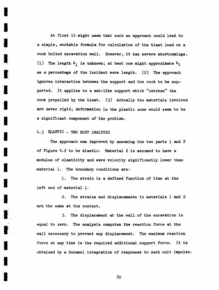
(l) The length is unknown; at best one might approximate
as a percentage of the incident wave length. (2) The approach
ignores interaction between the support and the rock to be sup
ported. It applies to a net-like support which "catches" the
rock propelled by the blast. (3) Actually the materials involved
are never rigid; deformation in the plastic zone would seem to be
a significant component of the problem.
U.3 ELASTIC - TWO BODY ANALYSIS
The approach was improved by assuming the two parts 1 and 2
of Figure k .2 to be elastic. Material 2 is assumed to have a
modulus of elasticity and wave velocity significantly lower than
material 1. The boundary conditions are:
1. The strain is a defined function of time at the
left end of material 1.
2. The strains and displacements in materials 1 and 2
are the same at the contact.
3. The displacement at the wall of the excavation is
equal to zero. The analysis computes the reaction force at the
wall necessary to prevent any displacement. The maximum reaction
force at any time is the required additional support force. It is
obtained by a Duhamel integration of responses to each unit impulse.
89
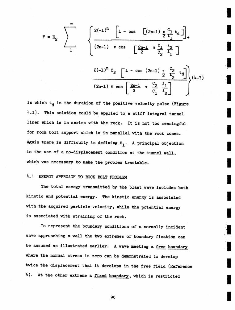
00
P * E ,<
2 (-l> ” f l - 008 [ ( *> - ! ) w7 17ra]l
(2n-l) ir cos j~2n-l ir f l f gC F "°2 -7 3
2 ( - l )n C« f l - cos (2n-l) ir C2 t 1____ L 2 T - dj (U-7)(2n-l) ir cos [2n-l
2, ik fi"1
°1 *2 J
in vhich t d i s the duration of the positive velocity pulse (Figure
Ir.l). This solution could be applied to a s t i f f in tegral tunnel
lin er vhich i s in se rie s with the rock. I t i s not too meaningful
for rock bolt support vhich i s in p a ra lle l v ith the rock zones.
Again there i s d ifficu lty in defining A principal objection
i s the use of a no-displacement condition at the tunnel v a i l ,
vhich vas necessary to make the problem tractab le .
U.U ENERGY APPROACH TO ROCK BOLT PROBLEM
The to ta l energy transmitted by the b la st vave includes both
kinetic and potential energy. The kinetic energy i s associated
vith the acquired p artic le velocity , vhile the potential energy
i s associated vith strain ing o f the rock.
To represent the boundary conditions of a normally incident
vave approaching a v a il the tvo extremes of boundary fixation can
be assumed as illu stra te d e a r lie r . A vave meeting a free boundnT*y
vhere the normal stre ss i s zero can be demonstrated to develop
twice the displacement that i t develops in the free f ie ld (Reference
6 ). At the other extreme a fixed boundary, vhich i s restric ted
90
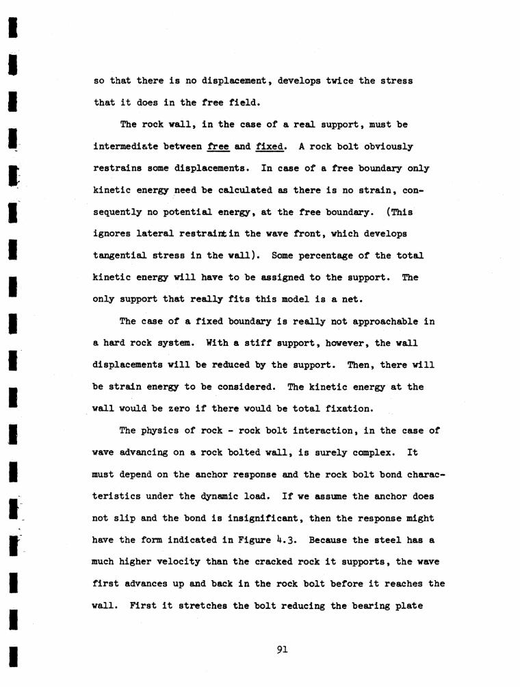
so that there is no displacement, develops twice the stress
that it does in the free field.
The rock wall, in the case of a real support, must be
intermediate between free and fixed. A rock bolt obviously
restrains some displacements. In case of a free boundary only
kinetic energy need be calculated as there is no strain, con
sequently no potential energy, at the free boundary. (This
ignores lateral restraint in the wave front, which develops
tangential stress in the wall). Some percentage of the total
kinetic energy will have to be assigned to the support. The
only support that really fits this model is a net.
The case of a fixed boundary is really not approachable in
a hard rock system. With a stiff support, however, the wall
displacements will be reduced by the support. Then, there will
be strain energy to be considered. The kinetic energy at the
wall would be zero if there would be total fixation.
The physics of rock - rock bolt interaction, in the case of
wave advancing on a rock bolted wall, is surely complex. It
must depend on the anchor response and the rock bolt bond charac
teristics under the dynamic load. If we assume the anchor does
not slip and the bond is insignificant, then the response might
have the form indicated in Figure U.3. Because the steel has a
much higher velocity than the cracked rock it supports, the wave
first advances up and back in the rock bolt before it reaches the
wall. First it stretches the bolt reducing the bearing plate
91
pressure. Later the wave displaces the wall stretching the bolt
and increasing the plate pressure at the same time. The first
response may be termed uncoupled as the bolt and the wall move
independently; the latter may be termed a coupled response as
the bolt is moved by the wall.
We will base the design approach on a determination of AT
(Figure U.3), the increase in bolt tension produced by the coupled
response. AT might be termed the maximum passive force increment
in the rock bolt. The procedure will be, approximately, to
multiply the average power of the wave in the rock by the transit
time of the wave in the rock bolt (tB ). The transit time of the
wave in the rock bolt is basic because some energy is leaving
the bolt while some is entering. The maximum duration in which
energy can be stored in the bolt, assuming the bolt to behave
elastically, is the transit time (tg) which equals the rock bolt
length divided by its velocity.
tB = (l»-8 )
where:
% is the rock bolt length
Cfi is the wave velocity in the bolt.|
That is, the latest time that energy, which enters the bolt at
time t , can still be stored in the bolt is T + tg.
•*+•1 Case 1: Only Kinetic Energy Considered
We will calculate the maximum kinetic energy of the
rock acquired by a momentum impulse beginning at time t and ending
92
at t + tfi. The momentum per unit area transmitted by the wave over time dt is odt, where o is the average stress of the wave
in the time interval (Figure U.U). Then the momentum vector
per unit area is
t * t + tBM = odt
t = T
T + tBP C V dt (U-9)
A simplified way to calculate the associated kinetic energy would
be by analogy to a rigid body. Then, the kinetic energy ejj is
ek = 1/2 MV2 (U-10)
where V is the incident particle velocity in Equation (4-9)*
(Case 2 to be considered later is more refined). Solving for the
magnitude of the particle velocity
V - I ¡S I A . . .—¡r (‘‘-idwhich gives
Ck - 1/2 Ul a 2 (ll_12)
The momentum vector has a component perpendicular to the
wall, and another parallel to the wall
M * M0 + Mr (U-13)
^ ^ i Me (H-lk)
93
A =» the area of the wave front which impinges on the wall of the
tunnel. If the rock bolts are in a square pattern with spacing
S, the wall area of interest is Ay ■ S^. Let a be the angle
between the normal (the radial direction) and the wave advance
direction, then
Also
and
then,
A = Ay cos a *
Mj. | = | M | cos a
Me | = I M I sin a
cos a
ck = 1/2
+ 1/2
o 2cos a -
2 2 Ay cos ans|M|2 sin2 a
|M|2 COg2 a
(^-15)
(1*-16)
(^-17)
The first term of Equation (U-17) gives the kinetic energy
associated with Mg which is to be dissipated parallel to the wall,
while the second term is the energy associated with S which is torbe dissipated perpendicular to the wall.
As a further simplification the kinetic energy associated
with Mg can be presumed to be tolerable because of the confinement
afforded by contiguous material.
The energy associated with Mr must be borne partly by the
rock bolts, partly by reflection of the momentum, and partly by
9k
/
internal energy absorption. Let k be the proportion of energy
which can be withstood by the rock system. Then the kinetic
energy to be taken by the bolting scheme is
c . (1 - k) A,2 co.11 a iMl2 r 2M
If the rock bolt length is l and the cross section area of the
rock bolts is A , the energy which can be taken by the bolt
assuming elastic behavior is (Figure 4.5):
e =11/2 + ^ ¿ 1 Agi (4-19)L E E Jk
where is the increase in bolt stress caused by the blast, and
is the bolt stress installed before the blast. If the initially
installed tension is T, the increase in tension ÀT required to
absorb the energy elastically is (other energy absorption
mechanisms are possible -- yielding anchor slip, or special
slipping bolts ) :
erbAsl [(AT)2 + 2TAT]
5 E (4-20)
Assuming a plastic behavior
e., * Te Ik rb p s (U-20)b
where i8 the plastic yield at load T (cf Figure 4.6)*
The mass M is calculated from the dimension of the rock body
assumed to be incapable of withstanding the blast without support.
95
This dimension is related to the rock holt if the bolts have
been properly designed. In any event the rock bolt length
defines the largest value of M. This gives
where p is the mass density of the rock.
The momentum ft can be computed by integration in a given
case. As noted, Reference 5 presents a typical wave form for
the velocity of a blast (Figure U.l). We will approximate this
by two straight lines as shown in Figure U.U. In these figures
R is the distance between the tunnel and the blast, while C is
the phase velocity of the medium.
As stated previously, the maximum duration energy is stored
in the bolt for tg equal to the transit time of the wave in the
bolt. It can be shown (Appendix 2) that the greatest momentum
that can be calculated by integration of Figure U.U over an
interval tg is as shown in Figure U.U, beginning at t such that V (r) * V (x + tB ). Let:
As shown in Appendix 2, the ruled area S of Figure k.k is given by
M = (As2) P (U-21)
(k-22)
S = Vmax (l-S2 ) (^-23)2
Since o * pCV, where C is the phase velocity and V is the particle
velocity of a solid, the momentum per unit area is then
( k -2 h )
T+tBM odt <>c W d (1-b2)
Substituting Reference 5's estimate for t^,
d ~ 2C (U-25)
where R is the distance from the blast, and C is the phase
velocity, the absolute value of momentum per unit area becomes
I A I „ oVmax ^ <1-S2)II E--- (U26)If there will be no failure, the kinetic energy associated
with the radial momentum component equals the elastic energy4r
absorbed by the rock bolt.
er “ erb
giving for an elastic rock bolt behavior
[-(l-k) S2 cos^
2p* -][ PRV___(1-B2) "12max ] As&TAT2 + TATI (U-27) 2E
The required increase in bolt tension is T given by:
[ a t2 + ta t] ^P [l-k| * W 1- s2) cos2 •
Vs_Roc. Material Blastbolt properties Characteristics
properties(lt-28)
97
where
E is the elastic modulus of the rock bolt
A_ is the area of the rock bolt s
S is the spacing of rock bolts (in a square pattern)
<- is the rock bolt length
p is the mass density of the rock
R is the distance from the blast
V is the maximum particle velocity of the incident blast m&xvave
a is the angle between the blast direction and the normal
to the rock wall
8 as defined in Equation (U-22)
k is a dimensionless coefficient indicating the percentage
of normally incident wave energy that the rock takes
without transference to the rock bolts, k is a
measure of the rock restitution, strength, and
plastic deformability. k would approach 0 for a
"plastic" zone where all.stresses corresponded to
limiting equilibrium and should approach 1 for a
hard unjointed and unweathered rock mass at inter
mediate or distant range. It also depends on the
blast intensity.
The increase in tension required to accommodate the blast
depends on the initial tension T. If T ■ 0, then AT is
98
lA R Vmax(l"e2) cos2 v (U-29)
If there is an initial tension T, then the quadratic equation can
be used to solve (U—28) for AT. Assuming a plastic behavior, er *
erb gives
(l-k) S2 Cos** a p R V (l-B2 ) max2pl u
= Te l A P s(U-30)
tep
Rock bolt energy
absorbator properties
Rock bolt properties
»(1-k), R V,max d-e2) Cos
Material Blast characteristics properties
A-31)
k.k.2 Caae 2: Total Work Considered
The above (Case l) assumed that only the momentum
component perpendicular to the wall needs to be considered in
calculating the energy to be absorbed by the rock bolt. Further
it assumes that the energy can be calculated from the momentum
by Equation A-12).
If the rock is deformable, the total work done on the
rock by the traveling wave may be a more fundamental quantity
on which to base analysis. A calculation for this case follows.
The total energy traveling during the transit time of
the rock bolt is equal to the work. Therefore,
99
T+tS
etotal “ ^
T
adU ( I t - 3 2 )
where U is the particle displacement and A is the area of the
wave considered.
The integration is contained in Appendix 2. The result is
where as before 3 is defined by Equation (U-22).
By analogy with the previous case we will divide the total
energy into a portion associated with the tangential component
of the wave motion Gq ' and a portion associated with the radial
component of the wave motion er '•
dU = Vdt
and
a a pCV
so that
T+tB
T
etotal = 3 ^ Vmax2 *d i1”**3) ( U - 3 U )
etotal * e0f + er ' ( -3 5)
100
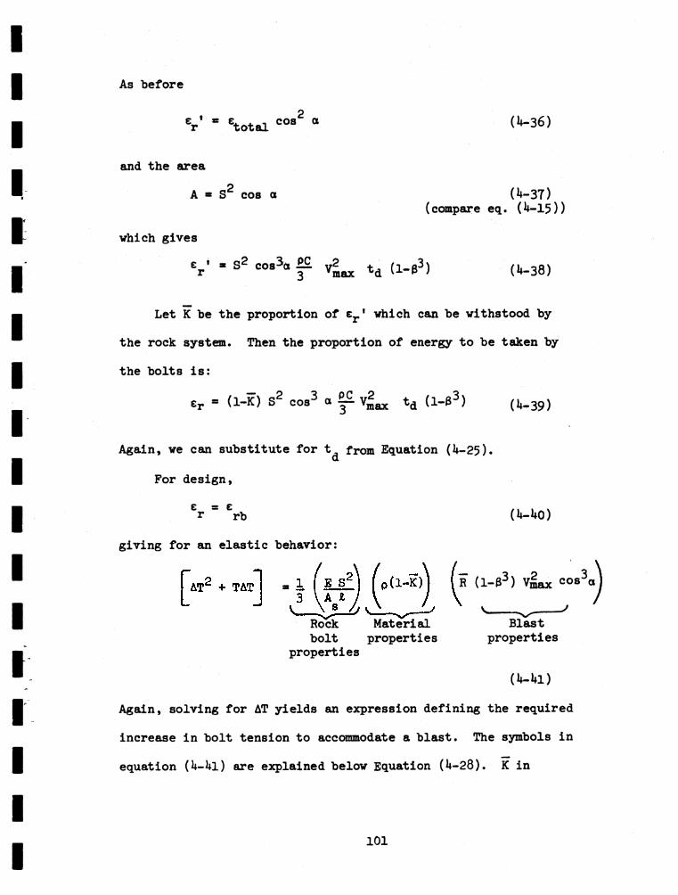
As before
etotal cos ( 1 36)
and the areaoA « S cos o (U-37)
(compare eq. (U-15))
which gives
V - S2 cos^o td (l-B3) (U—38)
Let K be the proportion of er ' vhich can be withstood by
the rock system. Then the proportion of energy to be taken by
the bolts is:
er = (1-K) S2 cos3 o V2^ td (l-S3 ) (U-39)
Again, we can substitute for t, from Equation (U-25).aFor design,
Er * Erb (U-UO)giving for an elastic behavior:
Rock Materialbolt properties
properties
R (1-B3 ) Vmax cos3«,
Blast ^ properties
(U-Ul)Again, solving for AT yields an expression defining the required
increase in bolt tension to accommodate a blast. The symbols in
equation (h—hi) are explained below Equation (h—28). K in
101
Equation (1*-Ul) must be different than k in Equation as
it is the proportion of the total energy that can be vi+nstood
by the rock in Equation (b— i»l).
For a plastic behavior, e * e givesr rb
TeP Cos 3o ( ^ g 3) (W»2)
Rock Rock Material Blastbolt bolt properties properties
energy properties behavior
k.5 DISCUSSION
Equations (lt-28) and ( U-l+1 ) could allow calculation of the
increase in bolt tension necessary to accommodate a blast. This
was the object of the analysis (compare with Figure U. 3).
According to the previous discussion, Equation (U-28) should be
closer to the correct calculation if the rock bolt system stiff
ness, as compared to the rock stiffness, is such that wall dis
placements are essentially unimpeded by the bolting pattern.
Equation (U-Ul) seems more appropriate in the case of a very stiff
rock bolt support scheme in which wall displacements are severely restricted.
This approach, however, assigns unknown rock properties to
a quantity k or K which might in fact be a non-linear function.
However, in the case of a nuclear blast the coefficients k and ÏC
depend heavily on the state of the rock, the support pressure, and
on the nature of the blast. They can be constant over a small
102
range of support pressure, and they can be very close to 1
when the support pressure is high.Some experimental data are available that allow a more
general relationship between the previous quantities and e
This chapter has calculated the energy of the traveling wave, which is, in itself a meaningful physical quantity. The next chapter will discuss how the actual support system will carry
this energy.
103
DIS
PL.
d
AC
GE
L. a
V
ELO
CIT
Y
F I G U R E 4.1
T Y P I C A L WAVE FORMS FOR DI RECT T R A N S M I T T E D GROUND SHOCK FROM E X P L OS I ONS.
FROM AMBRASSEYS AND H E l f ORON (1968) p. 221
101+
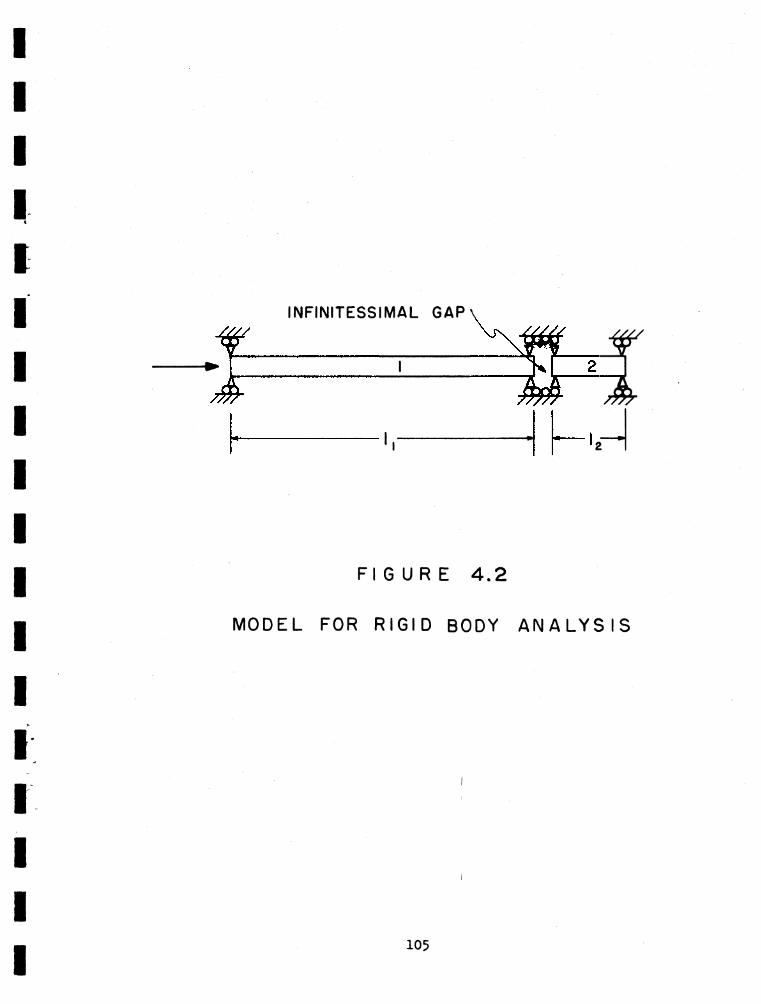
INFINITESSIMAL GAP
I
F I G U R E 4 . 2
MODEL FOR RIGID BODY ANA L Y S I S
105
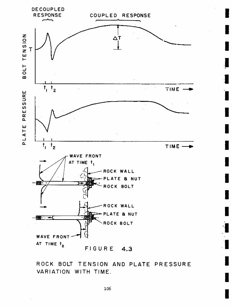
PL
AT
E
PR
ES
SU
RE
B
OLT
T
EN
SIO
N
DECOUPLEDRESPONSE C O U P L ED RESPONSE
WAVE FRONT AT TIME t,
WAVE F R O N T AT T IME t «
FI G U
ROCK W A L L
P L A T E 8 N U T
ROCK BOLT
R O C K WALL
P L A T E 8 NUT
ROCK B O L T
R E 4 . 3
ROCK BOLT T E N S I O N AND P L A T E P R E S S U R E VARI ATI ON WITH T I ME.
106
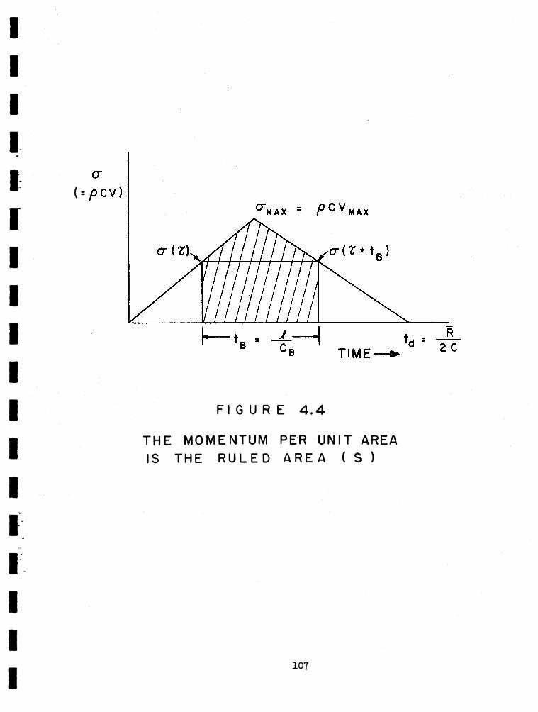
F I G U R E 4 . 4
T H E M OM EN TUM PER U N I T AREA IS T H E R U L E D A R E A ( S )
107
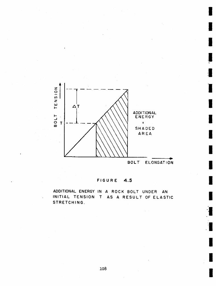
F I G U R E 4 . 5
ADDITIONAL ENERGY IN A ROCK BOLT UNDER AN INITIAL TENSION T AS A RESULT OF ELASTIC STRETCHING.
108
BO
LT
TEN
SIO
N
T
BOLT ELONGATION PER UNIT LENGTH
b= T Ag
FIG. 4 .6
PLASTIC YIELD ENERGY ABSORPTION BY THE ROCK BOLT
109
CHAPTER 5
EMPIRICAL APPROACH TO SUPPORT DESIGN AGAINST FLASTS
In this chapter the previously calculated energy quantities of
the propagating waves of the blast will be generalized to mf.tch
underground support for any kind of blast. Experimental data will
be used to find an empirical energy relationship between es , the
maximum energy that can be absorbed by the support system, and
er ', the energy normal to the wall that is transmitted by the
blast wave (compare equation (U—38) previous chapter).
5.1 DEFINITIONS
5.1.1 Wave Travel Time
In a nuclear explosion the duration t<j may not follow
the relationship of Equation (U-25). A more general form would be
where n is a constant of the type of explosive device used.
Examples
a. Data was taken from POR HOIO (draft copy), Omaha District,
Corps of Engineers, Protective Structures Branch.
110
Pile Driver Section Range (feet) td Blast ParticleWave Directi.vn Velocity
____________ __ MeasuredC Drift 9k0 106.8 1»0 fpsD Drift 8k0 90.6 53 fps
000 fps *4= st _ _ Rn T —Ztdc
C Drift: n = O.U95 D Drift: n = 0.51 nav = 0.5
b. Free field ground motion in granite measured in Pile Driver from data from W. R. Perret.
e Drift 9ko feet 66 ms 62.37D Drift 81*0 feet 62 ms 102.50
C - 18,000
C Drift: n = .79 D Drift: n ■ .75
n RtdC
5.1.2 Energy Absorption by the Support SystemThe total energy es that can be absorbed by the support
system has to be evaluated. In the rock bolt case it isT2*.
es = erb = ^rb ^s “ 2EA (5-2)where Xrb is the allowable energy absorption per unit of volume.
2In the case of ultimate strength design the second term 2EASis much smaller than the first and can be removed.
Ill
$•1.3 Energy Dissipation Time of the Support System
The blast can have a long positive duration ta (62 ms
to 106 ms in the previous examples). In these conditions the
support system might have the time to dissipate the first energy
part of the traveling wave before the arrival of the end of the wave.
This time tB is fundamental in the energy dissipation mechanism
and has been calculated previously in the case of rock bolt support.
tB *
where: l =
CB *
For other support methods another
, _LCBlength of the bolt
wave velocity in the rock bolt
expression for tg will be necessary.
5.2 RESULT OF THE PILE DRIVER TESTS
The 16' long rock bolts in C Drift were spaced at one bolt
per 3.25 square feet giving an ultimate support pressure Pr, ofBult
Bult92,000
3.25 X l U 192 psi
then pB ,— - =1.00 pounds/in'3 BRo
These results are all for a given experiment, which means the
weapon size is a constant. Thus the strain and the duration of
strain levels above some given value vary with the range according
112
to a definite function. To extrapolate the Pile Driver results
to sane other experiment, vhere strain and duration vary with
range according to a different function defined "by a different
weapon size, we will attempt to generalize the form of presentation
by calculating the energy per unit area that is tolerable.
The Pile Driver results can be expressed in the following
relationship
rB2R, A q ^ (5-3)
where: PB is the support pressure
RQ is the radius of the tunnel
cr ' is the traveling energy per unit area given in
the previous chapter (Equation h-36).
e0 is the energy per unit of area that can be
accepted without support.
e0 is a function of the rock properties and takes the place of the
quantities k and K of the previous chapter. This Equation (5-3)
can predict the safe-unsafe limit for all kinds of blasts once the
rock properties are given. Moreover the formula can be extended to
all kinds of supports.
$.2.1 General Empirical Energy Equation
Equation (5-3) can be written in a more general sense.
I 113
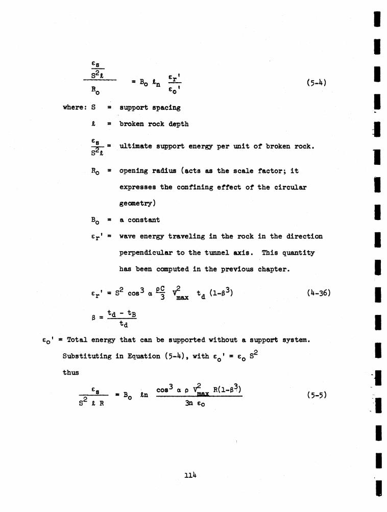
S21a Bo An
where: S 3 support spacing
A 3 broken rock depth
(5-*>
-2— 3 ultimate support energy per unit of broken rock.S ^ A
R0 3 opening radius (acts as the scale factor; it
expresses the confining effect of the circular
geometry)
B0 3 a constant
er' 3 wave energy traveling in the rock in the direction
perpendicular to the tunnel axis. This quantity
has been computed in the previous chapter.
er' 3 S2 cos3 a td (l-U3) (U-36)
e _ *d - tB td
eD' 3 Total energy that can be supported without a support system.A
Substituting in Equation (5—1*)» with e0* * eQ S thus
s2 n 3 B_ An cos'3 o p V“ R(l-B..IBM3n e0 (5-5)
I lk
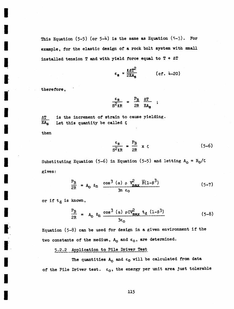
This Equation (5-5) (or 5-*0 is the same as Equation (5-3). For
example, for the elastic design of a rock holt system with small
installed tension T and with yield force equal to T + AT
AAT2 es 85 2Ei£ (cf. W20)
therefore,
es _ ATS2AR 2R EAg
AT is the increment of strain to cause yielding. EAg Let this quantity he called £
then
es- X -- « -- X £S2tR 2R
(5-6)
Substituting Equation (5-6) in Equation (5-5) and letting AQ = B0/£
gives:
7 / v ..2 — /. „3\(5-7)^ - A „ * n °°°3 («> P
or if td is known,
PB2R = A© *n
3n eQ
cos3 (a) pCV^WY td (l-e3) (5-8)3e0
Equation (5-8) can he used for design in a given environment if the
two constants of the medium, Aq and e0 , are determined.
5.2.2 Application to Pile Driver Test
The quantities Aq and e0 will he calculated from data
of the Pile Driver test. eQ , the energy per unit area Just tolerable
115
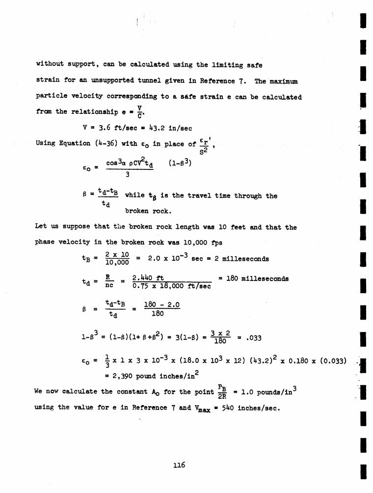
;
without support, can be calculated using the limiting safe
strain for an unsupported tunnel given in Reference 7. The maximum
particle velocity corresponding to a safe strain e can be calculated
from the relationship e ■
V * 3.6 ft/sec * 2*3.2 in/sec
Using Equation (l*-36) with e0 in place of ll! ,S2
cos3« pCV2^ (i-e3) e0 * ------ ----- i3
3 * while to is the travel time through thetdbroken rock.
Let us suppose that the broken rock length was 10 feet and that the
phase velocity in the broken rock was 10,000 fps
tB = 2 x 10 10,000
0= 2.0 x 10 sec »' 2 milleseconds
4 » _ mmR_ 2.UUO ft = 180 millesecondstd “ nc 0.75 x 18,000 ft/sec
3 =td-tfi 180 - 2.0td 180
1-83 * (l-3)(l+ B+B2) = 3(1-3) = 3 x 2180 = .033
*o * j x 1 x 3 x 10”3 x (18.0 x 103 x 12) (1*3.2)2 x 0.180 x (0.033)p■ 2,390 pound inches/in
We now calculate the constant Aq for the point 1- ® 1.0 pounds/in^2Rvising the value for e in Reference 7 and Vmax = 5l*0 inches/sec.
116
At this range
x _ __ * _ 16’ _ , 0 _ 62-1 _ 61t d = 62 ms, t B * ig-^doTn/s^T ~ l m 3 ' "62“ " 62
( l - 33) * 3(1 -$) * « k .9 x 10"2
and from Formula (5- 8 )
. . . 1 x 3 x 10”3 (5^0)2 .062 It .9 x 10-2 x (18 x 103 x 121.0 » A_ In --------------------------- --------------=----------------------- ---------
0 (3 ) (2.39 x 10³)
*o = * °*23 P°und/in3
Thus the Pile Driver data suggest a formula for the support pressure
required to insure stability of a tunnel as follows (cf. Equation (5- 6 ))
, o.23 *n 00,3 °3 x 2,390
(all units in pounds, inches and seconds)
5.3 HARDHAT DRIFT/
This can be checked against data from the Hardhat experiment
in an 8 foot diameter drift at a range of U57 feet supported by
5 foot long rock bolts. At this range the strain was 2.0 x 10“3;li j,
the maximum velocity at this range is therefore, 1.8 x 10 x 20 x 10“H =
36 ft/sec; t d = .ys' x l l boo * 0,° 3U 8econd; ^ ( l"e3) “ 2,7 x 10~2,
Then
117
psiP,.(D, 12) (0.23) tn ■Ol°~3)(36xl2)2(lfeao3xl2)(0.3l.)(2.7xl0-2)3 x 2390
PB « 22.0 x An (15.3)
Pb * 59.5 psiThe holts in this Hardhat drift were at 3 foot spacing, meaning the
required yield force per holt was
Ty = 9 x 1UU x 59.5 - 77,000 pounds
Since only 3/4" bolts were used, the gallery should have failed
according to the method of calculation. The rock in this Hardhat
drift broke to a depth of 1 1/2 to 2 feet.
5.4 CONCLUSION
An empirical relationship has been presented by the Omaha District
of the Corps of Engineers which gives the support pressure required
to preserve a given size of tunnel when subjected to a given level
of strain. By casting this relationship in the form of an energy
comparison it is possible to assess the effect of differing weapon
sizes and wave durations, thus the results of one experiment with
a given characteristic ground motion can be related to another
experiment with different wave parameters.
118
REFERENCES
1. Ambraseys, N. N. and Hendron, A. J., "dynamic Behavior of RockMasses". Rock Mechanics in Engineering Practice. Jg...i Wiley and Sons, New York, 1968. '
2. Bonssinesq, J., "Application des potentials it 1 etude de la equilibre et du movement des solides elastique", Gauthers-Viliars, Paris, 1895.
3. Duncan, J. M. and Goodman, R. E., "Finite Element Analyses of Slopes in Jointed Rock", Report No. TE-68-1, U. S. Army Engineers Waterways Experiment Station, Vicksburg, Mississippi, 1968.
1*. Ewoldsen, H. M. and McNiven, H. D., "On the Theory and Design of Rock Bolted Tunnels", Report No. 68-15, Structural Engineering Laboratory, University of California, Berkeley, 1968.
5. Goodman, R. E. "Analysis of Structures in Jointed Rock", Tech.Report No. 3, U. S. A m y Corps of Engineers, Omaha District, 1967*
6. Goodman, R. E., "Effects of Joints on the Strength of Tunnels",Tech. Report No. 5* U. S. Army Corps of Engineers, Omaha District,1968.
7. Jaeger, J. C. and Cook, G. W., Fundamentals of Rock Mechanics, sMethuen and Co. LTD., 1969.
8. Lang, T. A., "Rock Behavior and Rock Bolt Support in Large Excavations", Civil Engineering, Vol. 28, 1958.
9. Lang, T. A., Unpublished Course Notes for Rock Mechanics, 1965*
10. Kolsky, H., Stress Waves in Solids, Dover Publications, Inc.,New York, 1963.
11. Mindlin, R. D., "Force at a Point in the Interior of a Semi-infinite Solid", Proc. First Midwestern Conference of Solid Mechanics, University of Illinois, 1953.
12. Smart, J. D. and Heitmann, D. G., "Factors Which Influence Survival of Backpacked Sections Subjected to Nuclear Explosions", Operation Flint Lock, Event Pile Driver and Operation Nougat, Shot Hard Hat, to be published by U. S. Army Corps of Engineers, Omaha District, SECRET.
APPENDIX I
by Iraj Farhoomand
Elastic two body analysis applied to tunnel support problem
(see Chapter 3).
120

Assumptionsa) I and II are elasticb) Modulus of elasticity of I is different from modulus of elasticity ic) Wave is in the direction of the systemd) « *L
e) ^# l 2 1 x«—
»1¡2 - M 3
C1 C2 Aoo *1 Aoo *2 z k rX = 0
„29 U1 i 3 ui 2s3x2 4 3t2
(j) = ,xxC1
3ui.9x = p (t) for X *l,x- P(s) (1)
ou- 3u_3x
z3x for X = o ► *l,x" 2 ,x (2)
U1 = u2 for X = 0 — =► *1 - <t>2 (3)
u = 0 for
*2
(1)
(2)
( (3)
ou x -a, xA1 e + B e 'L
oux -ouxA2 e + B2 e
X = ¿2 = * = 0
with a, = — a» = — 1 C1 2 c2
P = a,ot t - o ne - e
Ol A1 - ax B1 - a2 A2 + a2 B2 =- 0
(4)
*1 - h = 0
A1 + B1 - A2 - B2 = 0
a ^ A n na2 e + b2 e = 0
(4)
121

Al “ C1 s- < V i ) - a ^
B1 e I e
(3) becomes i f we rep lace by i t s value
- V i - 2V iâ - e + B1 e + B! - Aj - B2 - 0
Í - “ V l -A y B 2 - M l e
1 - i - 2 0 .1 .1 + e 1 1
(m)
I f we rep lace A1 by i t s value in (2)
(2) g iv e s B1 = “2 A2 - \ h - P e“1 *1
a - 2 V i 1e -Il(n)
—ot 0 - a 0P l 1 iln A0 + n B - n 77“ e = mût A0 - mOL B0 - m e2 “ OL 2 2 2 2
(n - mCl ) A2 + (n + mo^) B2 »
A2 = - b2 e" 2a2Â2
- (n - mo^) B2 e-2 a2£2
1 -2V 1 , 1 -2V i ,e - 1\
■ - e - 1
- a £J
- 2 P e 1 X 1
-PL JL) B = - 2 P 1 1e
P e" a i Âl
B2 =- 2 P e“ V l
1, - 2a2 h \ f - 2a2Â2|n il - e 1 + md2 1 + eV '
1 . -2x -x 1 + e = e , x , - (e + e 'x ) = 2 e"x « X
But /- -2x “X , X -x N 0 -x . ,1 - e = e (e - e ) = 2 e sinh x
122
B„ = -2 P e-a^l
- ‘M i -a-A_ -(a.JL + M o)-a^ 4 e (sinh a^A^) e (sinh + 4 a2 e
(cosh Oj£^) (cosh 0.2^ 2 ^
B„ =
B„ *
A_ =
“OC A—
*2 ,x (V = a2 A2 e " a2 B2 6
F = E2 *2,* (V = E2 a2. a2Ä2 _a2Ä2 A2 6 - B2 e
F =- E2 s2 (P cx )
2 s M / M / M / Ä2c0 (sinh s — sinh s — - c . cosh s — (cosh s — 12 1 Cl / l c2 1 C1 c2
F =
123
tH j

Assumption; If c2 « (safe side)
P EF =
Assumption
c2
2
S = i (2 n-1) j 1 z
✓S1 i 2n_!
2
cI11
d_ds cosh x cosh s —
c2
1 G F
wG(w) wtF ^ 6
(w roots of F)
f
12k
+00 ,2 n - l V
-1acosh — I (cosh — |
( - 1 ) ° eo t
M 4 „no 2ii-l C1 . 12 W ~ i cos —y — * -s- TrC1 2 c2 K1
+00,2 n - l CL 7T
+ 2...( - D n
22 < 2 n - l 2 * ¿1c2 1 —
(2 n - l ) i r c . t
2 “ i « -1 * — s r ^
. 2 n - l n 22 *1 c° s — ^ * *7 *
+ 0 0
(2 n - l ) i r c _ t 2 c 2 ( - l , s in ------ j j — 2 -
, 2 n - l 2 . 21 ^22 c°s * j - n
F = 2 E„ ( - l ) nP (x ) s i n j
(2 n - l ) i r c 1 ( t - x )
2 JL dx
» . . 2n—1 1 . £22 t cos _ — * _ s
+ ( - 1) ” c .P ( ) s in
(2 n - l)7 r c2 ( t - x )
2 A, dx
¿2 cos2 n - l 2 . £1 1— ^ * 2 7 ”)
125
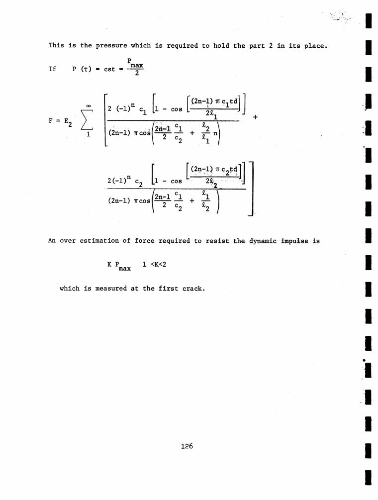
This is the pressure which is required to hold the part 2 in its place.
If P (t ) = cst max
F = E,2 (-1)“ cx 1 - COS
(2n-l) nr c. tdI 1 12 % x J J
(2n-l) ttcosI '2iHl- C12 C„
+ *2 \ 17 nl 2 i /
2(-l)n c2 |' |,1 - COS(2n-l) tt c2td^j* 2^2 4
(2n-l) tt cos I2n-l fl 2 c2
An over estimation of force required to resist the dynamic impulse is
K P 1 <K<2max
which is measured at the first crack.
126
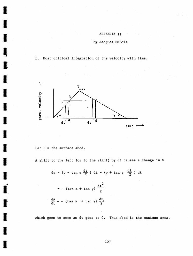
part,
velocity
APPENDIX IIby Jacques DuBois
1. Most critical integration of the velocity with time.
V
Let S = the surface abed.
A shift to the left (or to the right) by dt causes a change in S
ds * (v - tan a ) dt - (v + tan y ) dt
dt2= - (tan a + tan y)
= - (tan a + tan y)
which goes to zero as dt goes to 0. Thus abed is the maximum area
127
2. Value of the momentum integrated from to Tcr^t + tg where Tcr^t - a
in section (1) of this appendix;
time — — ---^
tB (1 - 6) td
giving
fcd " CBe = :----------
fcd
(1 - e> fcd _ vm ~ v fcd " vm
3 ym v
128
fcd id ci id/• _Momentum M = pc 1 vdt = pc / vdt - f vdt - i vdt
«yo J J JL o o t2 J
v tjs - m d (3v ) (3 tr) in L S . (Bv.) (8 (td - tr)> 2 o
32 vS1 + s2 = (tr + td - tr)
S - (S. + s 2) = Vm fcd g2 V fcd vm (1 " ß2) fcd
pcv t ,Momentum = ----2— SL (1 - g"6)
2
3. Integration of V dt the total energy
tBJlV
(1 - 3) td
t - (1 - 3) td
I 129
2 p 'd c i H -,E = p c J v 3d t = p c J v 2 d t - f v 2d t - J v 2d t = PC
2S o V "*
3 m Cs1 + s 2 >23 8vm
fcl “ o o $ \ - i -
J?ߣ3 vm 2 t d - ß ft e t r evm + % e ( t d - t r ) ßvm) (i - ß3)
130 I
DISTRIBUTION LIST
No. of Copies(Number of Copies of Report Shown in Parentheses) Form 1^73
Chief of Research and Development: Department of the Army;ATTN: CRDNCB, CRDSTI (l), CRDPES, CRDES (l); Washington,D. C. 20310 2
Chief of Engineers; Department of the Army; ATTN: CER (l),ENGAS-I (2), ENGAS-IL (1), ENGBR (l), ENGCE (l), ENGCW-E (2),ENGCW-EC (1), ENGCW-ED (l), ENGCW-EG (l), ENGCW-ES (l),ENGCW-RR (1), ENGCW-Z (l), ENGMC-D (l), ENGMC-DE, ENGMC-E (l),ENGMC-EA (1), ENGMC-ED (l), ENGMC-EP (1), ENGMC-ER (1),ENGMC-M (1), ENGME-E (l), ENGME-EF (l), ENGME-ER (l),ENGME-ET (l), ENGME-RD (2), ENGME-S (1), ENGML (1), ENGSA
Division Engineers, U. S. Army Engineer DivisionsHuntsville (2) North Pacific (2)Lower Mississippi Valley (2) Ohio River (2)Missouri River (2) South Atlantic (2)New England (2) South Pacific (2)North Atlantic (Resume only) Southwestern (2)
Directors, U. S. Army Engineer Division LaboratoriesNew England (2) South Atlantic (1)North Atlantic (2) South Pacific (1)North Pacific (2) Southwestern (2)Ohio River (2) Missouri River (2)District Engineers, U. S. Army Engineer Districts
Alaska (2) New Orleans (2)Albuqueroue (2) New York (2)Baltimore (2) Norfolk (2)Buffalo (2) Omaha (2)Charleston (2) Philadelphia (2)Chicago (2) Pittsburgh (1)Detroit (2) Portland (2)Fort Worth (2) Rock Island (2)Galveston (2) SacramentoHuntington (2) St. Louis (2)Jacksonville (2) St. Paul (2)Kansas City (2) San Francisco (2)Little Rock (2) Savannah (2)Los Angeles (2) Seattle (2)Louisville (2) Tulsa (2)Memphis (2) Vicksburg (2)Mobile (2) Walla Walla (2)Nashville (2) Wilmington
131
No. of Copies(Number of Copies of Report Shown in Parentheses) Fora ÏI+73
President; Mississippi River Commission; CE; P. 0. Box 80; Vicksburg, Mississippi 39180 (l)
Research Center Library; U. S. Army Engineer Waterways Experiment Station; P. 0. Box 631; Vicksburg,Mississippi 39180 (10)
U. S. Army Cold Regions; Research and Engineering Laboratory; (USA CRREL); Hanover, N. H. 03755 (l)
U. S. Army Engineer School Library; Thayer Hall(Bldg. 270); Fort Belvoir, Virginia 22060 1
Ballistic Research Laboratories; ATTN: AMXRD-BD;Aberdeen Proving Ground, Maryland 21005 1
Coastal Engineering Research Center; ATTN: Library;5201 Little Falls Rd. N. W.; Washington, D. C. 20016 1
U. S. Army Engineer Nuclear Cratering Group; LawrenceRadiation Laboratory; P. 0. Box 808; Livermore, Calif. 9^550 1
DEPARTMENT OF THE AIR FORCE
Research and Applications Br.; ATTN: AF/Preer;Directorate of Civil Eng.; HQ USAF; Pentagon;Washington, D. C. 20030 1
Office of Director of Defense Research and Engineering;ATTN: Director Strategic Weapons; Rocm 3E129; Pentagon,Washington, D. C. 20301 1
Headquarters, SAMS0 (AFSC); A1TN: MMHFI-Luedeking (l),XRTBN; Norton AFB, California 921*09 1
SAMS0/DEE; ATTN: William A. Platt; AF Unit Post Office;Los Angeles, California 900U5 1
DEPARTMENT OF THE NAVY
Naval Civil Engineering Laboratory; ATTN: TechnicalLibrary L31; Port Hueneme, California 9301+1 (l)
Naval Facilities Engineering Command; Navy Department;ATTN: William J. Bobisch, Chief Engineer; Washington,D. C. 20390 1
132
(Number of Copies of Report Shown in Parentheses)No. of Copies
Form lit 7 3
OTHER DOD AGENCIES
Advanced Research Projects Agency; ATTN: NuclearMonitoring Research Office; lUOO Wilson Bird.;Arlington, Va. 22209 1
Director; Defense Atomic Support Agency; Washington,D. C. 20305 (1)
Test Command; ATTN: TCDT-E; Sandia Base, New Mexico 87115 1
Administrator; Defense Documentation Center; Cameron Station;(12), Building 5; Alexandria, Virginia 2231**
Director of Defense Research and Engineering; ATTN:Assistant Director Nuclear Programs; Assistant Director Strategic Weapons; Technical Library; Washington, D. C.20301 3
OTHER GOVERNMENT AGENCIES
U. S. Bureau of Mines; ATTN: Leonard Obert, ScienceAdviser-Mining Research; Building 20, Denver Federal Center; Denver, Colorado 80225 (l)
U. S. Bureau of Mines; ATTN: J. R. McWilliams, Divisionof Mining Systems; Washington, D. C. 2021*0 (5)
U. S. Bureau of Reclamation; ATTN: M. H. Logan, Chief,Geology and Geotechnology Branch; Bldg. 67, Denver Federal Center; Denver, Colorado 80225 (l)
U. S. Bureau of Reclamation; ATTN: D. L. Misterek,Code 1512; Bldg. 56, Denver Federal Center, Denver,Colorado 80225 (l); Mr. G. B. Wallace (l)
U. S. Department of Commerce; N0AA - National Ocean Survey Lake Survey Center; 630 Federal Bldg. & U. S. Courthouse; Detroit, Michigan 1*8226 ( 2)
California Dept. Water Resources; ATTN: L. B. James,Chief Geologist; P. 0. Box 388; Sacramento, Calif. 95802 (l)
California Dept. Water Resources; ATTN: J. A. Wineland,Chief, Design Branch, Div. of Design & Construction;P. 0. Box 388, Sacramento, California 95802 (l)
133
(Number of Copies of Report Shown in Parentheses)No. of Copies
Form 1^73
OTHER GOVERNMENT AGENCIES (Gont'd)
Federal Highway Administration; bOO Seventh Street, S.W.; Washington, D. C. 20591 (l)
Federal Highway Administration; Office of Research;ATTN: W. J. Halstead, Chief, Materials Division;Washington, D. C. 20591 (l)
\
Highway Research Board; ATTN: Librarian; 2101 ConstitutionAvenue N.W.; Washington, D. C. 20bl8 (l)
U. S. Geological Survey; ATTN: H. W. Olsen, EngineeringGeology Branch; 3^5 Middlefield Road; Menlo Park,California 9b025 (l)
U. S. Geological Survey; ATTN: E. C. Robertson; AcornBldg.; 8001 Newell St.; Silver Spring, Maryland 20910 (l)
Tennessee Valley Authority; ATTN: R. B. Connelly,Manager's Office, Engineering Design and Construction;700 Union Bldg.; Knoxville, Tenn. 37902 (2)
Tennessee Valley Authority; ATTN: J. H. Coulson;300 Arnstein Bldg.; Knoxville, Tenn. 37902 (l)
FOREIGN OFFICE
Chief of Engineers; Department of the Army;ATTN: ENGME-AS; Washington, D. C. 2031b 1
FOR FORWARDING TO:
AWRE; Foulness Island; Southend-on-Sea; Essex, England 1
Canadian Forces Liaison Officer (Engr); USAMERDL,Fort Belvoir, Va. 22060 for: Dr, N. B. Hutcheon;Canadian Joint Staff; Department of Transport: Div. ofBldg. Research, National C Research Council of Canada;Ottawa; Construction Engineer; Air Service Branch;Ottawa, Ontario, Canada 5
Nova Scotia Technical College; ATTN: Dr. G. G. Meyerhof,Dept, of Civil Engineering; Halifax, N. S., Canada 1
13b
No. of Copies Fora 1^73(Number of Copies of Report Shown in Parentheses)
UNIVERSITY
1University of California; ATTN: R. E. Goodman,Assoc. Prof.; Dept, of Civil Engineering; U75 Davis Hall; Berkeley, California 9^720 (l)
University of California; ATTN: Lawrence RadiationLaboratory Technical Information Dept. L-3; P. 0. Box 808; Livermore, California 9^550 (l)
University of California; Los Alamos Scientific Laboratory; ATTN: Report Librarian; P. 0. Box 1663; Los Alamos,N. Hex. 875MColorado School of Mines; ATTN: John J. Reed, Dept, ofMining Engineering; Golden, Colorado 80U01 (l)
Cornell University; ATTN: G. A. Kiersch, Chairman;Dept, of Geological Sciences; 125 McGraw Hall,Ithaca, N. Y. 1U850 (l)
Colorado State University; Foothills Engineering Research Station; ATTN: Prof. K. S. Lane; Ft. Collins, Colorado80521 (1 )Cornell University; ATTN: Dr. D. A. Sangrey, Assoc. Prof.,Dept, of Geotechnical Engineering; School of Civil and Environmental Engineering; Ithaca, New York 1U850 (l)
Florida State University; ATTN: E. G. Henneke; School ofEngineering Science, Tallahassee, Florida 32306
Harvard University; ATTN: Prof. A. Casagrande; PierceHall; Cambridge, Mass. 02138
University of Illinois; ATTN: E. J. Cording; 2221 CE Bldg.,Urbana, Illinois 61801 (l); R. B. Peck; 2230 CE Bldg, (l)
University of Illinois; Dept, of Civil Engineering; ATTN: Dr. D. U. Deere (l); Dr. N. M. Nevmark (l); Prof. A. J.Hendron, Jr. (l); Metz Reference Roooi, B106 C. E. Bldg.; Urbana, Illinois 6l801 (l)
University of Illinois; Department of Geology; ATTN:Dr. F. A. Donath (l); F. D. Patton (l); Urbana, 111. 61801
Iowa State University; ATTN: L. V. A. Sendlein,Department of Earth Science; Ames, Iowa 50010 (1)
I 135
(Number of Copies of Report Shown in Parentheses)
UNIVERSITY (Cont*d)
Louisiana State University; ATTNj Dr. 0. A. Nance,Consultant to RAND and DASA; P. 0. Box 16006-LSU;Baton Rouge, La. 70803
Massachusetts Institute of Technology; ATTN: R. C.Hirschfeld, Room 1-330 (l); Asst. Prof. H. H. Einstein,Room 1-380 (1); Prof. W. F. Brace, Roam 5^-720 (l);Cambridge, Mass. 02139
University of Minnesota; ATTN: Prof. C. Fairhurst;Dept, of Civil and Mineral Engineering; Minneapolis,Minnesota 55^55 (l)
University of Missouri at Rolla; ATTN: Dr. N. B. Aughenbaugh, Chairman; Dept. Mining, Petr., & Geol. Engrg. (l);Dr. G. B. Clark; Director, Rock Mechanics & Explosives Research Center (l); Rolla, Missouri 65^01
University of New Mexico; Eric H. Wang Civil Engineering Research Facility; ATTN: Dr. E. Zvcyer; Dr. G. E.Triandafilidis; Mr. P. A. Abbott; Mr. D. E. Calhoun;P. 0. Box 188; University Station, Albuquerque, New Mexico 87106 H
City College of New York; Dept, of Civil Engineering;ATTN: Prof. C. A. Miller; New York, N. Y. 10031 1
Pennsylvania State University; Dept, of Architectural Engineering; ATTN: J. S. Futrick, Admin. Aide;101 Engineering "A" Bldg., diversity Park, Pa. 16802 (l)
Pennsylvania State University; ATTN: R. Stefanko,Assistant Dean, Earth & Mineral Sciences Continuing Education; 110 Mineral Sciences Building; University Park, Pa. 16801 (l)
Purdue University; School of Civil Engineering;ATTN: Prof. Wm. R. Judd; Lafayette, Indiana ¿7907 (l)
South Dakota School of Mines & Technology; Department of Mining Engineering; ATTN: Dr. E. Hoskins (l);Prof. E. H. Oshier (l); Rapid City, South Dakota 57701
University of Texas at Austin; Dept, of Petr. Engineering;ATTN: Dr. K. E. Gray; Austin, Texas 78712 (l)
No. of Copies Form 1^73
1
136

No. of Copies(Number of Copies of Report Shovn in Parentheses) Form 1473
UNIVERSITY (Confd)
Texas A & M University; Center for Tectonophysics;ATTN: Dr. Melvin Friedman (l); Prof. J. Handin,Director (l); College Station, Texas 77843
Texas A & M University; College of Geosciences; Center for Tectonophysics; College Station, Texas 77843 (l)
Utah State University; Engineering Experiment Station;ATTN: Dr. R. K. Watkins, Associate Director;Logan, Utah 84321 1
Virginia Polytechnic Institute; Mining Engineering Department; ATTN: Lawrence Adler (l); Dr. C. Haycocks (l);Blacksburg, Va. 24060
INDUSTRY
The Aerospace Corporation; P. 0. Box 5866; San Bernardino, California 92408; ATTN: S. B. Batdorf, B2/2020;M. Watson; W. Pfefferle (l) 2
Analytic Services, Inc.; ATTN: Geo. Hesselbacher;5613 Leesburg Pike; Falls Church, Va. 22041 1
Applied Theory, Inc.; ATTN: Dr. J. Trulio; 1010 WestwoodBlvd., Los Angeles, California 90024 1
AVC0 Systems Division; Research Library; 201 LowellStreet, Wilmington, Mass. OI887 1
Battelle Memorial Institute; ATTN: Dr. R. W. Klingensmith;505 King Avenue; Columbus, Ohio 43201 1
Bell Telephone Laboratories; ATTN: G. F. Weissmann,Roan 1A-105A; Mountain Avenue, Murray Hill, N. J. 07974 1
Bell Telephone Laboratories; ATTN: R. W. Mayo;Whippany Road, Whippany, N. J. 07981 1
Boeing Company - MASD Library; ATTN: 23-99 R. E. Shippfor L. E. Fleishman; P. 0. Box 3955; Seattle, Wash. 98124 1
Boeing Company - ATTN: J. A. Blaylock, 2-5410, 8C-4l;K. Levien, Orgn. 2-5511 M/S 89-70; Mr. H. G. Leistner,Aerospace Group, Research Division, M/S 89-70; P. 0. Box3999, Seattle, Washington 98124 3
137
No. of Copies Fora i r b(Number of Copies of Report Shown in Parentheses)
INDUSTRY (Contfd)
Boeing Company; ATTN: Technical Library; P. 0. Box3999; Seattle, Washington 9812It 1
Engineering Societies Library; ATTN: Howard Gordon;3t5 East l*Tth Street, New York, N. Y. 10017 (l)
General American Research Division; ATTN: Dr. L. B.Holmes; 7 ^ 9 N. Natchez Avenue; Niles, 111. 606U8 1
LIBRARY, General Electric Company Space & RESD Divs.,ATTN: Mr. L. Chasen, Manager; P. 0. Box 8555;Philadelphia, Pa. 19101 1
General Electric TEMPO; ATTN: DASIAC; P. 0. Drawer QQ,Santa Barbara, California 93102 1
General Motors Technical Center; ManufacturingDevelopment /33/; ATTN: W. M. Isbell; Warren, Mich. L8090 1
Gulf Radiation Technology; ATTN: H. R. Kratz;P. 0. Box 608; San Diego, California 92112 1
IIT Research Institute; 10 West 35th Street;ATTN: Document Library (l); Dr. K. E. McKee (l);Chicago, Illinois 6o6l6
Lockheed Missiles & Space Company, ATTN: Dr. R. E.Meyerott/C. C. Old; P. 0. Box 50U; Sunnyvale,California 9^088 2
Mueser, Rutledge, Wentworth & Johnston; ATTN: P. C.Rutledge; 1*15 Madison Avenue, New York, N. Y. 10017 1
N0AA Environmental Research Laboratories; ATTN: Dr. J. S.Rinehart; Boulder, Colorado 80302 1
The RAND Corporation; ATTN: Dr. H. L. Brode; Dr. C. C. Mow;1700 Main Street, Santa Monica, California 90U06 2
Research Analysis Corporation; ATTN: Documents Library;Route 123; McLean, Virginia 22101 1
Sandia Laboratories; ATTN: M. L. Merritt, Dept. 9150;W. R. Perret, Division 9111; P. 0. Box 5800,Albuquerque, N. M. 87115 2
138
Ho, Of Copies(Number of Copies of Report Shown in Parentheses) P o m 1^73
INDUSTRY (Cont*d)
Test Command, ATTN: TCDT-E; Sandia Base,New Mexico 87115 1
Shannon & Wilson, Inc.; ATTN: Dr. R. P. Miller;1105 N. 38th Street, Seattle, Washington 98103 (l);S. D. Wilson (1)
Southwest Research Institute; ATTN: R. C. DeHart;8500 Culebra Road; San Antonio, Texas 78228 1
Systems, Science & Software; ATTN: Document Control;P. 0. Box 1620; La Jolla, California 92037 1
TRW Systems (Rl/1138); ATTN: Norman Lipner;1 Space Park; Redondo Beach, California 90278 1
TRW Systems Group; ATTN: Dr. J. L. Merritt (l);F. A. Pieper; P. 0. Box 1310, San Bernardino,California 92U02 1
Paul Weidlinger, Consulting Engineer; 110 East 59thStreet, ATTN: Dr. M. L. Baron; New York, N. Y. 10022 1
Woodward-Clyde & Associates; ATTN: A. T. Harrigan,Librarian; P. 0. Box 2U075; Oakland, California 9^623 (l)
Woodward-Clyde & Associates; ATTN: R. L. McNeill;758 N. Batavia; Orange, California 92668 (l)
Woodward-Clyde & Associates, Inc.; ATTN: Dennis Leary;31 Orton Road; West Caldwell, New Jersey 07012 (l)
Woodward-Lundgren & Associates; ATTN: C-Y Chemg;P. 0. Box 21*075; Oakland, California 9^623 (l)
139
II
UNCLASSIFIEDSecurity C lassification
rr: • * ; ? t N . f
DOCUM ENT C O N T R O L D A TA - R & D(Security c la s s if ic a tio n o t t i t le , body o f abstrac t and indexing annotation must be entered when the o ve ra ll report Is c lase ilia d y
1. O R I G I N A T I N G A C T I V I T Y (Corporate author) 2a» R E P O R T S E C U R I T Y C L A S S ! Ft C A r f ë â
Omaha District, Corps of Engineers UNCLASSIFIEDOmaha, Nebraska 68102 2b. G R O U P
3. R E P O R T T I T L E
Static and dynamic Analysis of Rock Bolt Support
4. D E S C R I P T I V E N O T E S (Type o t report end In c lu s iv e detee)
Interim8. A U T H O R ( S ) (F irs t name, m idd le in i t ia l , le e t neme)
Richard E« Goodman and Jacques DuBois«. R E P O R T D A T E
January 19717«. T O T A L N O . O P P A O E S
lUll b . N O . O F R E F S
12B e . C O N T R A C T O R G R A N T N O .
DACAU5-67-C-OOI5 Mod. P0026. P R O J E C T N O .
UDM7Ö012A0K1TASK: 09
<*■ WORK UNIT: 002
»«. O R I G I N A T O R ' S R E P O R T N U M fe E R ( S )
Technical Report No. 6
9b. O T H E R R E P O R T N O (S ) ( A n y o t h e r n u m b e r s t h a t m a y b e a s a i g n e d t h i s r e p o r t )
10. D I S T R I B U T I O N S T A T E M E N T
Approved for public release; distributioi1 unlimited.
I I . S U P P L E M E N T A R Y N O T E S
Reference: Technical Reports Nos. 2,3 and 5s September 1966, 1967 and 1968; same originating agency
12. S P O N S O R I N G M I L I T A R Y A C T I V I T Y
Department of the ArmyOffice of the Chief of EngineersWashington, D. C. 20315
13. A B S T R A C T
This report describes progress in a continuing effort to develop and evaluate methods which can be used to design underground openings to survive blast loadings. It includes discussion of the action of rock bolts under static loads and considers aspects of the interaction between rock and rock belt under dynamic loads. Only computational methods were used in this study.
First, closed form solutions for point loads are summed and superimposed to examine stresses induced by patterns of rock bolts around tunnels in linearly elastic material. The stress fields are compared to rock strengths according to simplified failure criteria, to appreciate the relative strengthening effect of different combinations of bolt and rock parameters. It was found that very substantial bolt pressures are required, e.g., 10% of the maximum applied pressure, to restrict rock breakage in ideally elastic material.
Then elastic-plastic material behavior is considered. Stresses induced by unequilibrated line loadings on the inner circumference of the tunnel are used to simulate rock bolt patterns. It is found that the rock bolt strengthening effect can more easily be substantiated in veaker materials. For example, vhen rock inside the "plastic” zone was taken as cohesionless, less than lji of the blast pressure is a sufficiently high rock bolt pressure to provide significant strengthening effect.
dynamic considerations are discussed in terms of an energy balance for the case of a plane rock wall bolted in a regular pattern which receives a stress
p!nBr"ToS5r"77Sw3r^«^!Sc5?oSlvo5rMS9»rTJ! 51 !HiSBu?U U i m v h 1473 « M O t t t . r o i . i W Y u . « . . UNCLASSIFIED
USULABSIFUSP èecurlty Clamlficatlon
wave impulse from inside. The problem is examined in two ways: First acalculation is made of the kinetic energy of the system in the most serious increment of time during the response, assuming the holt to behave elastically. Then, the total vork during all of the blast response period is considered, presuming the bolt damage to be cumulative. The objective of these computations is to provide a basis for scaling survivability conclusions from one experiment to another. Reference is made to Hardhat and Piledriver experiments.
K E Y W O R D S L I N K A L I N KR O L E WT R O L E
Energy Absorption Elastic Analysis Elasto-Plastic Analysis Joint Influence Joint Properties Jointed Rock RockRock Bolts Rock Failure Rock Mechanics Rock Stress
III
Ihi UNCLASSIFIED
//so zs.III4IIIIIIIII1III

i
V ) aveG ì i


![REINFORCEMENT OF UNDERGROUND EXCAVATION WITH … bolt rod as a deformable rock bolt support component. The cylinder is located between the washer and the rock bolt nut [12], [23]](https://img.pdfslide.net/doc/110x75/5eaec2dc15c52910a23c3890/reinforcement-of-underground-excavation-with-bolt-rod-as-a-deformable-rock-bolt.jpg)