Research on the Common Rail Pressure Overshoot of Opposed ...€¦ · energies Article Research on the Common Rail Pressure Overshoot of Opposed-Piston Two-Stroke Diesel Engines Yi

energies

Article

Research on the Common Rail Pressure Overshoot ofOpposed-Piston Two-Stroke Diesel Engines

Yi Lu, Changlu Zhao, Zhe Zuo *, Fujun Zhang and Shuanlu Zhang

School of Mechanical Engineering, Beijing Institute of Technology, Zhongguancun South Street No.5,Beijing 100081, China; [email protected] (Y.L.); [email protected] (C.Z.); [email protected] (F.Z.);[email protected] (S.Z.)* Correspondence: [email protected]; Tel.: +86-10-6891-3637

Academic Editor: Chang Sik LeeReceived: 19 February 2017; Accepted: 20 April 2017; Published: 21 April 2017

Abstract: The common rail pressure has a direct influence on the working stability of Opposed-PistonTwo-Stroke (OP2S) diesel engines, especially on performance indexes such as power, economyand emissions. Meanwhile, the rail pressure overshoot phenomenon occurs frequently due to theoperating characteristics of OP2S diesel engines, which could lead to serious consequences. In orderto solve the rail pressure overshoot problem of OP2S diesel engines, a nonlinear concerted algorithmadding a speed state feedback was investigated. First, the nonlinear Linear Parameter Varying (LPV)model was utilized to describe the coupling relationship between the engine speed and the railpressure. The Linear Quadratic Regulator (LQR) optimal control algorithm was applied to designthe controller by the feedback of speed and rail pressure. Second, cooperating with the switchingcharacteristics of injectors, the co-simulation of MATLAB/Simulink and GT-Power was utilized toverify the validity of the control algorithm and analyze workspaces for both normal and specialsections. Finally, bench test results showed that the accuracy of the rail pressure control was inthe range of ±1 MPa, in the condition of sudden 600 r/min speed increases. In addition, the fuelmass was reduced 76.3% compared with the maximum fuel supply quantity and the rail pressurefluctuation was less than 20 MPa. The algorithm could also be appropriate for other types of commonrail system thanks to its universality.

Keywords: opposed-piston two-stroke diesel engine; common rail; pressure overshoot; LQR

1. Introduction

The Opposed-Piston Two-Stroke (OP2S) diesel engine concept, which has now been developedfor more than a century, came to being in the end of 19th century. Gilles was the first to propose theOP2S engine scheme with only one cylinder. Based on his research, Witting manufactured the firstopposed-piston engine using coal gas as fuel [1]. From then on, this technology was developed in manycountries and widely applied to different domains such as aviation, shipping and trucks. However, itsdevelopment was limited for a long time by the appearance of emission regulations [2]. In recent years,with the evolution of new materials, new techniques and internal combustion engine electronic controltechnology, many corporations including FEV, Advanced Propulsion Technologies (APT), EcoMotorsand Achates Power have launched research on OP2S engines and obtained satisfactory results [3–5],hence people have come to focus on this high power density two-stroke diesel engine format onceagain [6,7].

Benefiting from the application of electronic control, OP2S engines show stronger competitivenessin emission reductions and energy savings, especially for the electronic control high pressure commonrail system. This system had a more extensive practical value due to the superiority of its high injectionpressure and flexible injection parameters [8,9]. In order to meet the anticipated higher emission

Energies 2017, 10, 571; doi:10.3390/en10040571 www.mdpi.com/journal/energies

http://www.mdpi.com/journal/energies

http://www.mdpi.com

http://www.mdpi.com/journal/energies

Energies 2017, 10, 571 2 of 23

regulation requirements of the future, the common rail system has to supply a more accurate controlmethod for the engine combustion process and reduce the pollution generation. The key point ofcontrolling fuel injection quantity precisely is to realize the control of the combustion process. Thefuel injection quantity of common rail systems is determined by both rail pressure and injectionduration. Under the influence of high pressure operation conditions and the self-structure features ofcommon rail systems, a major pressure fluctuation would be generated inside the injector chamberwhile the needle valve of the injector is opening or closing, and the pressure wave would spreadinside the system. Catania et al. [10] studied the dynamic characteristics resulting from the pressurewave spread of common rail injection systems, and they found that the pressure fluctuation of theinjector entrance caused by water hammer was remarkable and it took a long time to recover fromit. Henein et al. [11] studied the injection characteristics and pressure fluctuation of the common railinjection system of diesel engines. They pointed out that practical injection duration was longer than thecommand duration with the rising rail pressure, which could have impact on the fuel quantity accuracy.Bianchi et al. [12] indicated the necessity of correcting the fuel injection quantity due to the pressurefluctuation characteristics inside the common rail system. On the other hand, it is also necessary tostudy rail pressure control strategies, for the reason that the accuracy of fuel-injection quantity can begrievously affected by the stability and responsiveness of the rail pressure. At present, rail pressurecontrol strategies mainly adopt the methodology combining feedforward control, open loop controland fuzzy Proportion Integration Differentiation (PID) control, and it also adjusts relevant parametersby monitoring the system working conditions in real time. By utilizing the feedforward rail pressurecontrol methodology based on the parameter self-regulation fuzzy PID algorithm, Ouyang [13,14]achieved good control effects and could satisfy the accuracy requirements of rail pressure control.Huang and Song from Shanghai Jiaotong University [15] developed a high pressure common railsystem named GD-1 with their colleagues and studied control strategies in depth. Xu and Wang [16]came up with a composite control strategy which could switch automatically between cascade controland open loop control. Their strategy appropriately solved the problem that rail pressure varied withthe change of engine working conditions, which made rail pressure respond rapidly and precisely.Zhou [17] developed a control system for high pressure common rail systems and put forward a newcylinder detection technology.

However, the OP2S diesel engine uses a hydraulic-mechanical hybrid output method, which hasan impact on the control of common rail pressure. Engine speed suddenly increases while the loadof the hydraulic pump falls sharply, then the engine speed control algorithm comes into action andimmediately reduces the fuel injection quantity, thus the engine speed would drop to a reasonablerange. In this situation, a prompt increase of speed causes an abrupt increase of fuel supply frequencyof the high pressure pump leading to a sharp rise in rail pressure. Even if the switch range of asolenoid valve could be adjusted by a conventional rail pressure control PID algorithm, a severe delaywould occur which results in a sudden rail pressure increase. Meanwhile, the engine control systemwould appropriately reduce the fuel injection quantity due to the speed rise. Under the synergy ofthese two aspects, the rail pressure would bump up and threaten the safety of the whole fuel system.Although the fuel injection quantity could be accurately maintained by the engine control system,depending on the injection adjustment characteristics as well as by adjusting the injection durationafter the rail pressure increased rapidly, the increase of injection pressure and decrease of injectionperiod would influence the injection rate, combustion and switching characteristics of the solenoidvalve, thus immediately influencing the working conditions, combustion stability and exhaust gasdeterioration. Although partial common rail systems could adjust their dynamic responsiveness byinstalling Pressure Control Valves (PCVs) at the exit of the high pressure pump, this slowed up thehigh-speed response characteristics. This technology is therefore not universally used yet. Meanwhile,the on-off of a proportional overflow valve would intensify the pressure fluctuation inside the railand impact the injection accuracy. Therefore, it is significant to study how to come up with a controlalgorithm to decrease the rail pressure overshoot by using other types of control feedback structures,

Energies 2017, 10, 571 3 of 23

without changing any oart of the existing structure of the common rail system components. Amongthe options optimal control algorithms might therefore be more suitable for common rail systems.

Through the feedback of state parameters of controlled objects, optimal control methods obtainoptimal effects and broad stability margins by coordinating the control expense and state indexes.Nowadays they play a vital role in engine control applications. Li and his co-workers [18,19] controlledthe engine speed and made it approach the expected value by making use of a linear prediction controlmethod and quasi-infinite time domain nonlinear model prediction control method. Fialho et al. [20]designed a self-adaptative active suspension controller and achieved an ideal operation result viathe combination of a linear parameter-variety controller and a nonlinear back-stepping controller.Kjergaard et al. [21] adopted an input-output linearization strategy and sliding mode control, andconducted elaborate comparative trails within classical PID control method and Linear QuadraticRegulator (LQR) control method. Yu et al. [22] demonstrated that engine torque control based onnonlinear model prediction control had good responsiveness, by means of comparing and analyzingthe direct injection engine torque control precept under feedback linearization, nonlinear modelprediction control as well as gain scheduling LQ optimal control. Furthermore, a direct relationshipbetween the rise of rail pressure and the increase of engine speed in common rail systems was beenfound. By utilizing a double-parameter speed-pressure-pressure control algorithm rather than theprimary single-parameter pressure-pressure control algorithm, the stability control requirement forrail pressure of an OP2S diesel engine could be better met. Therefore, optimal control theory, especiallythe LQR theory, could be appropriately applied to control the rail pressure. In the way of coordinatingthe control between different parameters such as engine speed and injection quantity, a decent controleffect is implemented with broad stability margin and good performance.

In order to meet the air-fuel mixture accuracy requirements under the impact of engine speed andload, the injection quantity must be measured precisely under the control of injection pressure andtiming. That is, research on control algorithms is influenced by the whole fuel injection system, so it isnecessary to establish a control-oriented model of a common rail injection system. Paolo et al. [23,24]built a flow nonlinear equilibrium model of common rail systems, and a simplified model of theinternal rail flow from the perspective of engineering practice. They also came up with a simplifiedmodel of a sliding mode control method and figured that the method was appropriate for stabilitycontrol of the common rail system nonlinear characteristics. Catania et al. [25] came up with a simplelumped parameter model of system vibration phenomena through a phenomenological analysis. Theyalso put forward a referenced simplified model aiming at one-time fluctuation effect, based on whichthe fuel quantity could be amended. This method is representative fuel quantity control of commonrail systems at present. Di Gaeta et al. [26,27] utilized a sliding mode method to control rail pressure aswell. For the purpose of stability control of rail pressure, they established a more detailed mathematicalmodel of a common rail system. Nevertheless, the most difficult part of the sliding mode controlmethod is the control signal step, which results in chattering phenomena. On account of the inherentfluctuation characteristics of rail pressure, the application of this method was partially limited.

In this paper, a common rail system mathematical model addressing the control strategy and anonlinear Linear Parameter Varying (LPV) model used to reflect the coupling relationship betweenthe engine condition and the rail pressure were established, which aimed at the problem that railpressure might suddenly increase because of a sudden change of engine speed in an OP2S dieselengine. A LQR control algorithm for speed feedback optimal generalized scheduling control wasput forward, which was based on the LPV model. In order to achieve a favorable control result onrail pressure, a MATLAB/Simulink and GT-Power co-simulation model was used to design referablecontrol parameters in offline mode. In addition, the control parameters and engine speed as wellas rail pressure were controlled concertedly. This turned out to achieve a wide stability margin andgood consistency.

Energies 2017, 10, 571 4 of 23

2. Experimental System

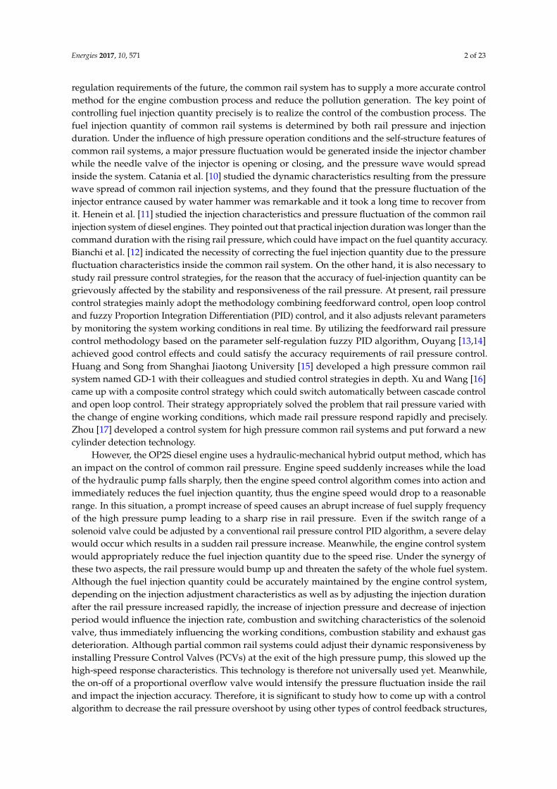
The development of the common rail system required original system experiments andcalibrations on the component test bench, in order to accomplish some steady tests of the injectionand pressure fluctuation characteristics. These processes could also verify and test the stability andperformance of the common rail control algorithm. Generally, a common rail component test bench iscomposed of an injection system pump rig, pressure sensors with both high and low sensitivity, currentclamp, a high-speed data acquisition system and fuel single injection equipment. After completing thecomponent experiments and verification, the overall test could be conducted, which mainly focusedon performance parameters, such as engine power, torque, dynamic variation and control performanceindexes. Meanwhile, some other parameters like cooling water temperature, oil temperature, intake airtemperature and pressure etc. ought to be monitored to adjust the control parameters in real time andprotect the engine from malfunctions. The engine test bench was universally made up of a completemotor, dynamometer, cooling circulatory system and monitoring system. The experimental prototypetest bench and measurement equipment are illustrated in Figure 1.

Energies 2017, 10, 571 4 of 23

2. Experimental System

The development of the common rail system required original system experiments and calibrations on the component test bench, in order to accomplish some steady tests of the injection and pressure fluctuation characteristics. These processes could also verify and test the stability and performance of the common rail control algorithm. Generally, a common rail component test bench is composed of an injection system pump rig, pressure sensors with both high and low sensitivity, current clamp, a high-speed data acquisition system and fuel single injection equipment. After completing the component experiments and verification, the overall test could be conducted, which mainly focused on performance parameters, such as engine power, torque, dynamic variation and control performance indexes. Meanwhile, some other parameters like cooling water temperature, oil temperature, intake air temperature and pressure etc. ought to be monitored to adjust the control parameters in real time and protect the engine from malfunctions. The engine test bench was universally made up of a complete motor, dynamometer, cooling circulatory system and monitoring system. The experimental prototype test bench and measurement equipment are illustrated in Figure 1.

Figure 1. Experimental prototype test bench and measurement equipment.

3. Common Rail System Model and Rail Pressure Control Algorithm

3.1. Common Rail System Model

3.1.1. OP2S Configuration

The OP2S diesel engine uses a hydraulic hybrid output method, which gets rid of the cylinder head. Each two pistons share one cylinder with a head in a level symmetrical layout and the flat combustion chamber is composed of two piston top surfaces and the cylinder wall. The injector, which injects the fuel into the combustion chamber from one side, was installed beside the cylinder jacket. It has only two strokes in a cycle and utilizes a uniflow scavenging system. The air inlet and outlet were both controlled by two pistons to accomplish the opening and closing motions, and these pistons promoted their own connecting rod mechanism respectively in order to drive the crankshaft

Figure 1. Experimental prototype test bench and measurement equipment.

3. Common Rail System Model and Rail Pressure Control Algorithm

3.1. Common Rail System Model

3.1.1. OP2S Configuration

The OP2S diesel engine uses a hydraulic hybrid output method, which gets rid of the cylinderhead. Each two pistons share one cylinder with a head in a level symmetrical layout and the flatcombustion chamber is composed of two piston top surfaces and the cylinder wall. The injector, whichinjects the fuel into the combustion chamber from one side, was installed beside the cylinder jacket.It has only two strokes in a cycle and utilizes a uniflow scavenging system. The air inlet and outletwere both controlled by two pistons to accomplish the opening and closing motions, and these pistonspromoted their own connecting rod mechanism respectively in order to drive the crankshaft by thesynchronizing mechanism. The engine structure is shown in Figure 2 and the parameters of the engineare listed in Table 1.

Energies 2017, 10, 571 5 of 23

Energies 2017, 10, 571 5 of 23

by the synchronizing mechanism. The engine structure is shown in Figure 2 and the parameters of the engine are listed in Table 1.

Figure 2. Configuration of OP2S diesel engine.

Table 1. Parameters of the OP2S diesel engine.

Parameter Item (Units) Value Number of cylinders (-) 2 Cylinder diameter (mm) 100

Stroke (mm) 110 Displacement (L) 3.4

Phase difference of the opposed-piston (°CA) 17 Maximum power (kW) 80 (2400 rpm) Maximum torque (Nm) 420 (1600 rpm)

Nominal compression ratio (-) 22 Angle of intake valve open (°CA) 116 Angle of intake valve close (°CA) 110

Angle of exhaust valve open (°CA) 100 Angle of exhaust valve close (°CA) 113

3.1.2. Fuel System Model

The configuration of the fuel system of the engine is shown in Figure 3. It consists of a low and a high-pressure circuit, including the fuel tank, a low pressure gear pump connected with the crankshaft, a high-pressure plunger pump with an electro-hydraulic proportional delivery valve, a common rail and the injector. An inline electric low pressure gear pump takes the fuel out of the tank and injects it into a low-pressure cycle. After being throttled by an electronic-hydraulic proportional valve which was driven by a Pulse Width Modulation (PWM) square wave current, adequate fuel is supplied to the high pressure pump. The nominal rail pressure was reached during compression of the high pressure pump piston and the fuel was then delivered to the pump-to-rail pipe in order to maintain the common rail pressure stability. Subsequently, the injector, which was linked to the high pressure fuel pipe and common rail, would conduct the injection process under Electronic Control Unit (ECU) control according to the injection requirements.

Figure 2. Configuration of OP2S diesel engine.

Table 1. Parameters of the OP2S diesel engine.

Parameter Item (Units) Value

Number of cylinders (-) 2Cylinder diameter (mm) 100

Stroke (mm) 110Displacement (L) 3.4

Phase difference of the opposed-piston (◦CA) 17Maximum power (kW) 80 (2400 rpm)Maximum torque (Nm) 420 (1600 rpm)

Nominal compression ratio (-) 22Angle of intake valve open (◦CA) 116Angle of intake valve close (◦CA) 110

Angle of exhaust valve open (◦CA) 100Angle of exhaust valve close (◦CA) 113

3.1.2. Fuel System Model

The configuration of the fuel system of the engine is shown in Figure 3. It consists of a low and ahigh-pressure circuit, including the fuel tank, a low pressure gear pump connected with the crankshaft,a high-pressure plunger pump with an electro-hydraulic proportional delivery valve, a common railand the injector. An inline electric low pressure gear pump takes the fuel out of the tank and injects itinto a low-pressure cycle. After being throttled by an electronic-hydraulic proportional valve whichwas driven by a Pulse Width Modulation (PWM) square wave current, adequate fuel is suppliedto the high pressure pump. The nominal rail pressure was reached during compression of the highpressure pump piston and the fuel was then delivered to the pump-to-rail pipe in order to maintainthe common rail pressure stability. Subsequently, the injector, which was linked to the high pressurefuel pipe and common rail, would conduct the injection process under Electronic Control Unit (ECU)control according to the injection requirements.

Energies 2017, 10, 571 6 of 23Energies 2017, 10, 571 6 of 23

Figure 3. A block scheme of the common rail injection system for diesel engines.

Like in the common rail system of an OP2S diesel engine, the strong nonlinearities caused by the complex flow of fuel resulted in difficulties for designing the fluid dynamic model, and an excessively detailed consideration could not help us to design a control algorithm. Thus the choice of model parameters and empirical formulas during modeling was based on the adaptability of the control target. Referring to [23], the model was divided on account of control volume, fuel dynamic pressure was described through combining together Newton’s motion law, the equation of continuity and the momentum equation. The bulk modulus formula of fluids was utilized to establish the flow-pressure differential equation, including high-pressure pump, common rail and fuel injector, based on the fuel pressure of different components in the common rail system [21]. Then, the relevant mathematical model was obtained. Fuel compressibility could be expressed by the bulk modulus formula:

f

d

d

pK

v v= −

(1)

It could be approximated by an empirical formula as:

f 1200 (1 0.6 )600

pK = ⋅ + ⋅

(2)

From (1), the following formula could be obtained:

f d

d

dp K v

dt v t= − ⋅

(3)

where, dv/dt took account of the inflow qin and outflow qout, and the volume changed dV/dt resulted from mechanical motion. Thus, Formula (3) could be written as:

fin out

d( )

d

dp K Vq q

dt v t= − ⋅ − +

(4)

V is a constant volume for all the elements in the common rail system, except the high pressure pump, therefore, it could be canceled. Both qin and qout could be obtained from the law of conservation of energy. The general flow formula of fuel flowing through the fuel orifice was as follows, which was based on Bernoulli’s Equation:

Figure 3. A block scheme of the common rail injection system for diesel engines.

Like in the common rail system of an OP2S diesel engine, the strong nonlinearities caused by thecomplex flow of fuel resulted in difficulties for designing the fluid dynamic model, and an excessivelydetailed consideration could not help us to design a control algorithm. Thus the choice of modelparameters and empirical formulas during modeling was based on the adaptability of the controltarget. Referring to [23], the model was divided on account of control volume, fuel dynamic pressurewas described through combining together Newton’s motion law, the equation of continuity and themomentum equation. The bulk modulus formula of fluids was utilized to establish the flow-pressuredifferential equation, including high-pressure pump, common rail and fuel injector, based on the fuelpressure of different components in the common rail system [21]. Then, the relevant mathematicalmodel was obtained. Fuel compressibility could be expressed by the bulk modulus formula:

Kf = −dp

dv/v(1)

It could be approximated by an empirical formula as:

Kf = 1200 · (1 + 0.6 · p600

) (2)

From (1), the following formula could be obtained:

dpdt

= −Kfv· dv

dt(3)

where, dv/dt took account of the inflow qin and outflow qout, and the volume changed dV/dt resultedfrom mechanical motion. Thus, Formula (3) could be written as:

dpdt

= −Kfv· (dV

dt− qin + qout) (4)

V is a constant volume for all the elements in the common rail system, except the high pressurepump, therefore, it could be canceled. Both qin and qout could be obtained from the law of conservation

Energies 2017, 10, 571 7 of 23

of energy. The general flow formula of fuel flowing through the fuel orifice was as follows, which wasbased on Bernoulli’s Equation:

q = sgn(δp) · c · A

√2|δp|

ρ(5)

where δp represents the pressure difference between both sides of the sectional area. The mathematicalmodel of the high pressure pump, common rail and injector of the OP2S diesel engine common railsystem could be established by using the above modeling principles.

3.1.3. High-Pressure Pump Model

A CP1H3 high pressure pump was chosen for this common rail system. Due to the complexityof its working principle, it should be simplified while modeling. Inside the triple plunger pump,pumping occurred three-times during one rotation of the camshaft. As a consequence, the rotationspeed of the camshaft should rise up to three times while the fuel should be supplied by only oneplunger in order to simplify it.

The plunger chamber volume of the high pressure pump varied with the camshaft rotation.Combined with the camshaft shape lines, the plunger chamber volume could be expressed as:

Vp(α) = Vp0 − Ap · sp(α) (6)

Considering the rate of change, the equation below could be obtained after taking the derivativeof Equation (6):

dVp

dt= −Ap ·

dsp

dt= −Ap · 2πn ·

dsp

dα(7)

where Vp0 represents the chamber volume when the plunger was at the Bottom Dead Center (BDC)

position, and the engine crankshaft was driven by the belt at a 1.125-fold rotation speed.On the basis of plunger distance variation curve related to camshaft shape lines, the fitting formula

could be obtained as:sp(α) = [2.85− 2.85 cos(0.01745α)]× 10−3 (8)

Taking the derivative of Equation (8), the following expression was obtained:

dsp(α)

dα= 4.97 sin(0.01745α)× 10−5 (9)

The pressure differential equations in each plunger chamber of the high pressure pump could beobtained as follows relating to the modeling principles:

.pp = −Kf

V(−Ap · 2πn ·

dhp

dθ+ qs − qr) (10)

After the fuel flows past the gear pump, the stepped fuel returned to the valve and the highpressure fuel pump solenoid valve were connected in parallel, which kept the fuel pressure of thesolenoid valve inlet stable and pg was around 0.5 MPa. This insured that system could work normally.The flow via the solenoid valve is as follows:

qs = sgn(pp − pg)cp Ap

√2∣∣pp − pg

∣∣ρ

· uPWM (11)

where qr could be obtained from the following equation:

qr = sgn(pr − pp)cr Ar

√2∣∣pr − pp

∣∣ρ

(12)

Energies 2017, 10, 571 8 of 23

3.1.4. Common Rail Pipe Model

Essentially, a common rail is a long, tubular, high pressure container, which stores highpressure fuel inside and distributes high pressure fuel to each injector through a fuel injection pipe.Meanwhile, the rail reduces the pressure fluctuation caused by the fuel injection procedure and fuelsupply procedure.

Considering that there is no rail deformation and no volume variation, two injectors installed inthe circumferential direction in each cylinder of the OP2S diesel engine could inject fuel at the sametime. The common rail pressure differential equation could then be obtained as:

.pr =

Kf(pr)

Vr(qr − 2 · qi,k) (13)

where, k = 1, 2, 3, 4 represent four injectors, respectively.Besides:

qi,k = sgn(pr − pi,k)ci,k Ai,k

√2|pr − pi,k|

ρ(14)

3.1.5. Fuel Injector Model

In the injector modeling process, the pressure chamber volume was regarded as approximatelyconstant. Thus, the pressure differential equation of injector pressure chamber could be obtained as:

.pi,k =

Kf(pi,k)

Vi,k(qi,k − qcyl,k) (15)

and qcyl,k could be obtained by the following equation:

qcyl,k = sgn(pi,k − pcyl,k)ci,kET,k Ai,k

√√√√2∣∣∣pi,k − pcyl,k

∣∣∣ρ

(16)

3.1.6. Fuel Quantity-Torque Transformation Model

The injection process of a common rail system is not totally independent from engine speed andload, and the fuel supply quantity is influenced by the engine speed and the injection quantity isinfluenced by load, which could cause a pressure fluctuation in the common rail. Therefore, the stateof the common rail system is directly related to the engine working conditions. However, consideringthat the engine combustion process is complicated and it is difficult to control the combustion processtimely and precisely in the actual control, it is thus quite significant to set up a simplified conversionmodel of the fuel quantity-torque faced with control implemention, which could satisfy the controlrequirements of the rail pressure overshoot problem of the common rail system. According to therelationship between engine speed and load, the conversion model of fuel quantity-torque of OP2Sdiesel engine could be simplified as:

.n =

1JEngine

(TEngine − Tload − Tf

)(17)

where JEngine represents the moment of inertia of the engine crankshaft, TEngine represents theindicated torque, Tload represents the load caused by the fuel pump, oil pump, water pump and otherattachments. Tf represents the load caused by friction and lubrication while the engine is working.

Energies 2017, 10, 571 9 of 23

Experimental calibration for mechanical losses of the OP2S diesel engine was conducted byutilizing an indicator diagram. According to the experimental data obtained on the test bench shownin Table 2, the fitted equation of drag torque and engine speed is:

Tf = 0.23 · n− 90.89 (18)

Table 2. Experimental data of the OP2S diesel engine.

Engine Speed(r/min)

Indicated Torque(N·m)

Effective Power(KW)

Mechanical Losses(KW)

Torque Losses(N·m)

900 11.111 0 11.111 117.9091200 20.962 4.712 16.250 166.8231400 32.103 10.995 21.108 218.9921600 46.007 18.848 27.159 274.606

The indicated power of the engine could be expressed as:

Pi = qcyl,k · i · Hu · ηit · n/60 (19)

where Hu represents the low heating value of diesel, in kJ/mg units i represents the number ofcylinders, ηit represents the indicated thermal efficiency, qcyl,k represents the cycle fuel injectionquantity, in mg/cyc units.

Indicated torque was expressed as:

TEngine = 9550 · qcyl,k · i · Hu · ηit/60 (20)

From the formula, the indicated torque of the engine was proportional to the cycle fuel injectionquantity. Considering that:

KT = 9550 · i · Hu · ηit/60 (21)

The expression could be transformed into:

TEngine = KT · qcyl,k (22)

According to the parameters of the OP2S diesel engine, the equation could be integrated as:

.n =

1JEngine

[2 · KTETci Ai

√2pr

ρ− (0.23n− 90.89)− Tload

](23)

3.2. Rail Pressure Control Algorithm

Considering that the common rail mathematical model has a high order and a complex form, andthe nonlinear factors make it more difficult to design the control algorithm, therefore, a simplifyingand linearizing model became a necessary objective in order to design the controller.

Currently, PID control algorithms have been widely applied for rail pressure control, but thecontrol delay problem caused by the calculation of control parameters under the state of rail pressureovershoot still exists. According to the mathematical model, it could be found that rail state isinfluenced by parameters such as speed, pressure, etc. Reaction speed and precision of the controlsystem could be enhanced with the speed feedback addition under the rail pressure control. The controltype using both rail pressure and speed as double parameter feedback has the same construction asthe classical optimal control.

Optimal control was the representative fruit of modern control theory, which gave the optimalcontrol effect of both control cost and state index harmonization, so the LQR scheduling control

Energies 2017, 10, 571 10 of 23

algorithm based on state space and the PID control algorithm optimized by optimal control areintroduced as follows.

3.2.1. Simplification of Common Rail Mathematics Model

In this paper, the major research direction was the study of influence of the speed fluctuationon rail pressure. Rail pressure was established by balancing the fuel supply flow and fuel injectionflow. The model of the high pressure fuel pump was simplified because of its complexity and toughcomputation process for fuel supply flow. The high pressure fuel pump supplied fuel three times ineach cycle of the camshaft, and it was directly proportional to speed frequency. Meanwhile, it wasinfluenced by the PWM signal which was used to control the solenoid valve so that the fuel supplyflow from the pump could be simplified using Equation (24):

qs =n60· 3 ·Vp · uPWM (24)

Like the pump, the fuel injection flow from the injector was also simplified. The injection flowrate could be obtained as follows while the pressure in injector pressure chamber was considered to beapproximately equal to that in the rail:

qcyl,k = ci,kET,k Ai,k

√2|pr|

ρ(25)

where the rail pressure pr and speed n were chosen as two states, and the system state equation couldbe obtained by:

.pr =

Kf(Pr)Vr

( n60 · 3 ·Vp · uPWM − 2 · ETci Ai

√2prρ )

.n = 1

JEngine

[2 · KTETci Ai

√2prρ − (0.23n− 90.89)− Tload

] (26)

Considering the coupling relationship between state variables and control variables, acorresponding transformation should be conducted on Equation (24), so the rail fuel quantity wastransformed into:

qs =n60· 3 ·Vp −

n60· 3 ·Vp · uPWM (27)

After the transformation, the two state parameters, namely rail pressure pr and speed n wererespectively written as x1, x2. The output parameter was still rail pressure pr, and it is written as y.Substituting other parameters of the OP2S diesel engine, the state space form of the system could beobtained as:

[ .x1.x2

]= a

−0.088 · ET

√1pr

0.456

0.1 · ET

√1pr

−0.29

[ x1

x2

]

+b

[−0.456n0

]uPWM −

[0

1.25

]Tload

y =[

1 0][ pr

n

] (28)

During the realization process of the OP2S rail pressure control, the integral error betweenreactive system current state and target state could be defined as the system error expansion, namedξe, according to the servo compensation design method. Coordination control of speed, fuel quantityand rail pressure without static error and using classical weight function-optimal control calculationmethod, the off-line design controller could be realized, by the influence of torque disturbance of

Energies 2017, 10, 571 11 of 23

load, uncertainty and model simplification compensated by the state parameters. After designing thedimension expansion of servo compensation, the system state space equation was as follows:

.x1.x2.ξe

= a

−0.088 · ET

√1pr

0.456 0

0.1 · ET√

1pr

−0.29 0

−1 0 0

x1

x2

ξe

+ b

−0.456n00

uPWM

y =[

1 0 0] x1

x2

ξe

(29)

uLQR = −Kp · x1 − Kn · x2 − Ke · x3 + Kp · pd (30)

3.2.2. LPV Linearization of the Common Rail Space Model

It could be found out that the state equation in a common rail system is influenced by thetime-variant and nonlinear parameters pr and ET via simplification of the rail model. With the controlof state feedback, the classical linear control method guarantees the system stability, but no consistencyof control effect. Therefore, the LPV method was adopted in this study for solving the problems ofcontrol system design that was affected by time-variant parameters, and achieving a stable controlof the rail pressure. With the method, some foreign experts and scholars had made efforts on thevehicle control system modeling and control domain. This was applied in the air intake system ofdiesel engines in [28] and in the time-variant parameter identification of gasoline engines in [29].In [30,31], a LPV-based scheduling method, specific to wetted wall engine parameters and enginespeed time-variant parameters was put forward. By utilizing group design of PID and PID controlparameters, the control problem of the influence of time-variant parameters to the nominal modelduring dynamic processes could be solved.

If the state matrix of a finite-dimensional system is the function of time-variant vector parameters,this sort of system is collectively called a LPV system. The time-variant vector parameter in LPV isa bounded set which can measure the specific values in real time without variety track prediction.In controller design problems of both linear time-invariant systems and linear time-variant systems,making the most of measurable information about the measurable time-variant parameters in thesystem and designing a control system with the study conclusion of linear control theory were the keypoints of utilizing the LPV system.

Directed at the rail pressure control problem, the pressure is influenced by the injection quantityand supply quantity, where injection quantity is a nonlinear function of the rail pressure state pr

and the time-variant measurable fuel injection pulse width ET. The fuel injection pulse width has atime-variant characteristic because of its variation under different engine conditions. Meanwhile itwas also influenced by wide rail pressure fluctuation and nonlinear variation under certain conditions.As a consequence, the rail pressure must be controlled by harmonizing the engine speed and injectionquantity to guarantee a stable rail pressure and to restrain the impact of rail pressure overshoot. Thecontrol principle of LPV aimed at common rail systems is shown in Figure 4. The control system woulddetect the current pressure state pr by a pressure sensor installed at the end of the common rail, andthe control deviation e was obtained by subtracting the target pressure pd from the current pressure pr.Weighted integral calculations were made on control deviation e, and finally the results are summedup to get the control parameter. The control parameter could control the electric current of the throttlevalve and adjust the opening angle of the valve through use of a duty cycle. Thus the goal of adjustingthe pressure could be attained.

Energies 2017, 10, 571 12 of 23

Energies 2017, 10, 571 12 of 23

end of the common rail, and the control deviation e was obtained by subtracting the target pressure pd from the current pressure pr. Weighted integral calculations were made on control deviation e, and finally the results are summed up to get the control parameter. The control parameter could control the electric current of the throttle valve and adjust the opening angle of the valve through use of a duty cycle. Thus the goal of adjusting the pressure could be attained.

Common railPump Fuel Flow

Fuel injection quantity & ET

prpd

Ke(pr, ET)*∫edt

Kn(pr, ET)

Kp(pr, ET)

uPWM

n

e

-

-

-

+

-

Figure 4. LPV control principle.

There were two nonlinear parameters (pr, ET) in the 3 × 3 matrix of Equation (22), which present the time-varying problem of the coefficient matrix while using the previous solution method based on the original equation. A unit gain coefficient of control variable could not be obtained. However, both of the time-varying nonlinear parameters (pr, ET) were measurable parameters. Referring to the LPV method, these measurable parameters could be substituted into the primary equation for solving, and the coefficient table, namely Kp(pr, ET), Kn(pr, ET), Ke(pr, ET) , which was directly related to those two parameters(pr, ET). This table could be updated by a look-up table program during the control implementation process, and the control equation can be shown as:

LPV p r r n r e r p r d( , ) ( , ) ( , ) ( , )u K p ET p K p ET n K p ET e dt K p ET p= − ⋅ − ⋅ + ⋅ + (31)

Hereby, for each certain condition of pr and ET, there must be a corresponding control solution that can satisfy the control expectations. The control parameters confirmed the control characteristic parameter group of the state feedback control variable K and the time-variant measurable parameters pr and ET via off-line design. The rail pressure could be controlled by different maps based on these parameters. In other words, on the basis of the LPV method, the controller parameters could be obtained by utilizing a linear control method to solve nonlinear control problems with the off-line design.

3.2.3. LQR Scheduling Control Algorithm Based on LPV Model

The LQR optimal control method possesses the advantage of computing the feedback control gain matrix [32] by providing a whole set of systems based on optimal control theory. Compared with general optimal control problems, linear quadratic type optimal control problems have two distinct features. First, most research objects of optimal control problems are multi-input multi-output dynamic systems, including single-input single-output types as an exceptional case. Second, the performance of the research system was comprehensive, flexible and practical.

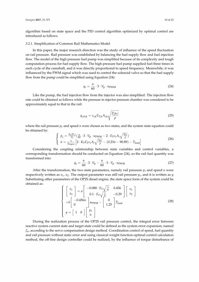
The LQR scheduling control algorithm was designed to solve the rail pressure overshoot problems based on the LPV model. Simulation and validation experiments were completed to obtain the final controller by revising the weight function. Figure 5 shows the design process.

The OP2S diesel engine common rail system has a target pressure of 60~120 Mpa under different conditions. While 60 ≤ pr ≤ 140 MPa, the step value was chosen as 20. Fuel injection characteristics were between 500 to 2500 μs and the step was chosen as 500 μs. Each pr and ET in different states were calculated with the LQR control parameter method. The rail pressure, speed and servo compensation state feedback parameter were respectively represented as Kp, Kn, Ke.

Figure 4. LPV control principle.

There were two nonlinear parameters (pr, ET) in the 3 × 3 matrix of Equation (22), which presentthe time-varying problem of the coefficient matrix while using the previous solution method basedon the original equation. A unit gain coefficient of control variable could not be obtained. However,both of the time-varying nonlinear parameters (pr, ET) were measurable parameters. Referring to theLPV method, these measurable parameters could be substituted into the primary equation for solving,and the coefficient table, namely Kp(pr, ET), Kn(pr, ET), Ke(pr, ET) , which was directly related to thosetwo parameters (pr, ET). This table could be updated by a look-up table program during the controlimplementation process, and the control equation can be shown as:

uLPV = −Kp(pr, ET) · pr − Kn(pr, ET) · n + Ke(pr, ET) ·w

e dt + Kp(pr, ET)pd (31)

Hereby, for each certain condition of pr and ET, there must be a corresponding control solutionthat can satisfy the control expectations. The control parameters confirmed the control characteristicparameter group of the state feedback control variable K and the time-variant measurable parameterspr and ET via off-line design. The rail pressure could be controlled by different maps based onthese parameters. In other words, on the basis of the LPV method, the controller parameterscould be obtained by utilizing a linear control method to solve nonlinear control problems withthe off-line design.

3.2.3. LQR Scheduling Control Algorithm Based on LPV Model

The LQR optimal control method possesses the advantage of computing the feedback controlgain matrix [32] by providing a whole set of systems based on optimal control theory. Compared withgeneral optimal control problems, linear quadratic type optimal control problems have two distinctfeatures. First, most research objects of optimal control problems are multi-input multi-output dynamicsystems, including single-input single-output types as an exceptional case. Second, the performance ofthe research system was comprehensive, flexible and practical.

The LQR scheduling control algorithm was designed to solve the rail pressure overshoot problemsbased on the LPV model. Simulation and validation experiments were completed to obtain the finalcontroller by revising the weight function. Figure 5 shows the design process.

The OP2S diesel engine common rail system has a target pressure of 60~120 Mpa under differentconditions. While 60 ≤ pr ≤ 140 MPa, the step value was chosen as 20. Fuel injection characteristicswere between 500 to 2500 µs and the step was chosen as 500 µs. Each pr and ET in different states werecalculated with the LQR control parameter method. The rail pressure, speed and servo compensationstate feedback parameter were respectively represented as Kp, Kn, Ke.


Figure 5. Design flow of the LQR scheduling control algorithm based on the LPV model.

The parameters Q and R were selected as:

[ ]1 0.1 0.1

= 0.1 1 0.1 = 1

0.1 0.1 1000

Q R

，

(32)

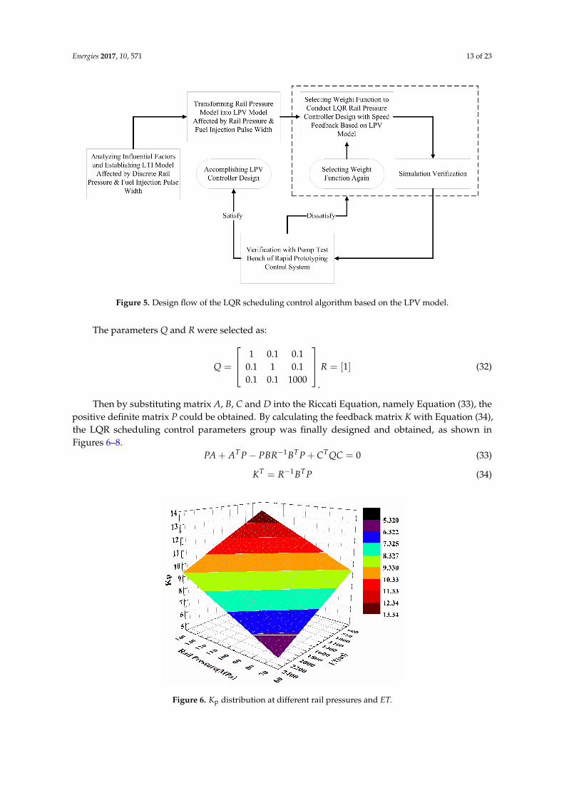
Then by substituting matrix A, B, C and D into the Riccati Equation, namely Equation (33), the positive definite matrix P could be obtained. By calculating the feedback matrix K with Equation (34), the LQR scheduling control parameters group was finally designed and obtained, as shown in Figures 6–8.

1 0T T TPA A P PBR B P C QC−+ − + = (33)

1T TK R B P−= (34)

Figure 6. Kp distribution at different rail pressures and ET.



Q =

1 0.1 0.10.1 1 0.10.1 0.1 1000

,

R = [1] (32)

Then by substituting matrix A, B, C and D into the Riccati Equation, namely Equation (33), thepositive definite matrix P could be obtained. By calculating the feedback matrix K with Equation (34),the LQR scheduling control parameters group was finally designed and obtained, as shown inFigures 6–8.

PA + AT P− PBR−1BT P + CTQC = 0 (33)

KT = R−1BT P (34)

Energies 2017, 10, 571 13 of 23



[ ]1 0.1 0.1

= 0.1 1 0.1 = 1

0.1 0.1 1000

Q R

，

(32)

Then by substituting matrix A, B, C and D into the Riccati Equation, namely Equation (33), the positive definite matrix P could be obtained. By calculating the feedback matrix K with Equation (34), the LQR scheduling control parameters group was finally designed and obtained, as shown in Figures 6–8.

1 0T T TPA A P PBR B P C QC−+ − + = (33)

1T TK R B P−= (34)

Figure 6. Kp distribution at different rail pressures and ET. Figure 6. Kp distribution at different rail pressures and ET.


Figure 7. Kn distribution at different rail pressures and ET.

Figure 8. Ke distribution at different rail pressures and ET.

3.2.4. Optimal Control PID Control Algorithm

The PID control algorithm has been optimized and the control principle is shown in Figure 9. The control system would detect the current pressure state pr by a pressure sensor installed at the end of the common rail, and the control deviation e was obtained by subtracting the desired pressure pd and the current pressure pr. Multiplication and integral calculations were made on control deviation e with different weights, and the results finally summed to get the control parameter. The control parameter could control the electric current of the throttle valve and adjust the opening angle of valve through the form of a duty cycle. Thus the goal of adjusting the pressure could be reached. The characteristic was that the integral coefficient was defined as the dimension expansion coefficient Ki, the proportionality coefficient was defined as Kp, which was the same as the system setup, and controller design was conducted by utilizing state feedback theory. Because that variable design parameters only contained the output state feedback and the integral of output state feedback, other state control effects are lacking in some aspects compared with an n-dimensional full-state feedback controller. Zhu [33] has studied in depth optimal control with PID control algorithms. Referring to his method, the PID and LQR control algorithms were combined in this paper. While Proportion (P) has the same definition as the pressure feedback coefficient Kp, integration (I) has the same definition as the error integral feedback coefficient Ke. Because of the lack


Energies 2017, 10, 571 14 of 23




The PID control algorithm has been optimized and the control principle is shown in Figure 9. The control system would detect the current pressure state pr by a pressure sensor installed at the end of the common rail, and the control deviation e was obtained by subtracting the desired pressure pd and the current pressure pr. Multiplication and integral calculations were made on control deviation e with different weights, and the results finally summed to get the control parameter. The control parameter could control the electric current of the throttle valve and adjust the opening angle of valve through the form of a duty cycle. Thus the goal of adjusting the pressure could be reached. The characteristic was that the integral coefficient was defined as the dimension expansion coefficient Ki, the proportionality coefficient was defined as Kp, which was the same as the system setup, and controller design was conducted by utilizing state feedback theory. Because that variable design parameters only contained the output state feedback and the integral of output state feedback, other state control effects are lacking in some aspects compared with an n-dimensional full-state feedback controller. Zhu [33] has studied in depth optimal control with PID control algorithms. Referring to his method, the PID and LQR control algorithms were combined in this paper. While Proportion (P) has the same definition as the pressure feedback coefficient Kp, integration (I) has the same definition as the error integral feedback coefficient Ke. Because of the lack



The PID control algorithm has been optimized and the control principle is shown in Figure 9. Thecontrol system would detect the current pressure state pr by a pressure sensor installed at the end ofthe common rail, and the control deviation e was obtained by subtracting the desired pressure pd andthe current pressure pr. Multiplication and integral calculations were made on control deviation e withdifferent weights, and the results finally summed to get the control parameter. The control parametercould control the electric current of the throttle valve and adjust the opening angle of valve through theform of a duty cycle. Thus the goal of adjusting the pressure could be reached. The characteristic wasthat the integral coefficient was defined as the dimension expansion coefficient Ki, the proportionalitycoefficient was defined as Kp, which was the same as the system setup, and controller design wasconducted by utilizing state feedback theory. Because that variable design parameters only containedthe output state feedback and the integral of output state feedback, other state control effects arelacking in some aspects compared with an n-dimensional full-state feedback controller. Zhu [33] hasstudied in depth optimal control with PID control algorithms. Referring to his method, the PID andLQR control algorithms were combined in this paper. While Proportion (P) has the same definitionas the pressure feedback coefficient Kp, integration (I) has the same definition as the error integralfeedback coefficient Ke. Because of the lack of feedback loop, the engine speed feedback coefficient Kn

Energies 2017, 10, 571 15 of 23

could only be 0, and the system could perform the calculations by setting Kn as a constant 0. Thus theoptimal PID control parameters could be theoretically obtained.

Energies 2017, 10, 571 15 of 23

of feedback loop, the engine speed feedback coefficient Kn could only be 0, and the system could perform the calculations by setting Kn as a constant 0. Thus the optimal PID control parameters could be theoretically obtained.



prpd

Ke*∫edt

Kn≡0

Kp

uPWM

n

Kpe

-

-

-

+

-

Figure 9. Control principle of PID optimized by optimal control.

3.3. Analysis of Rail Pressure Overshoot

3.3.1. Co-Simulation Model

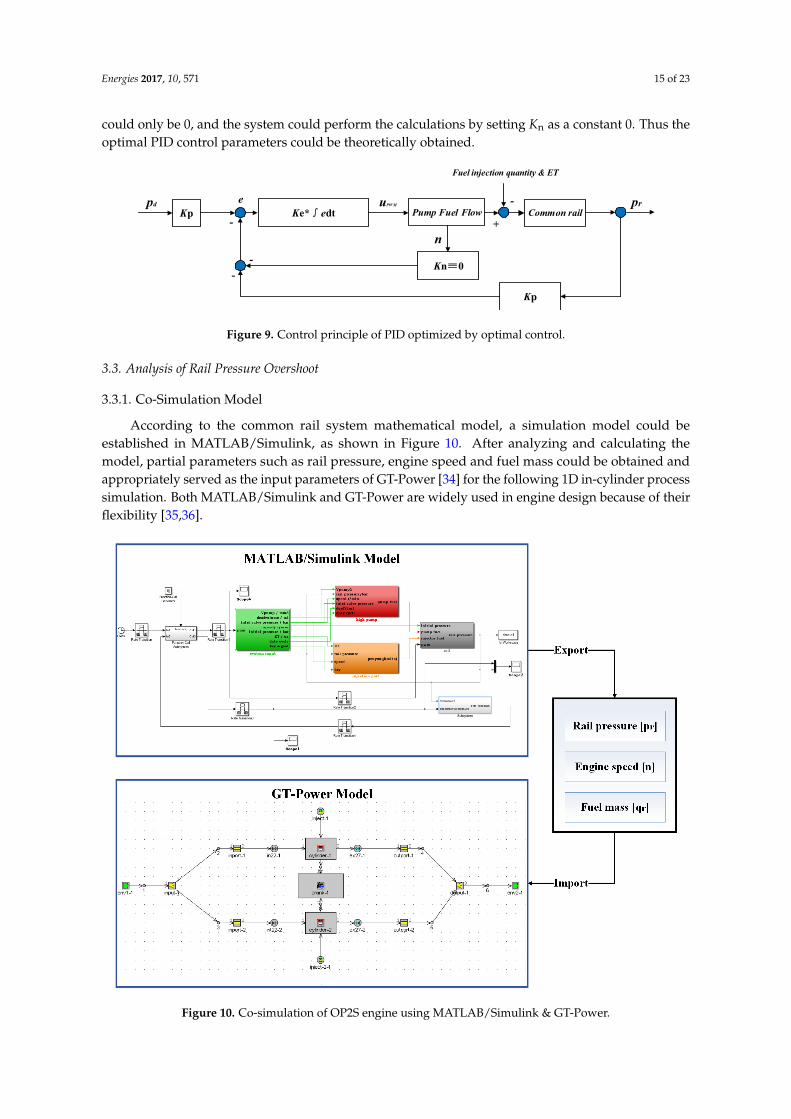
According to the common rail system mathematical model, a simulation model could be established in MATLAB/Simulink, as shown in Figure 10. After analyzing and calculating the model, partial parameters such as rail pressure, engine speed and fuel mass could be obtained and appropriately served as the input parameters of GT-Power [34] for the following 1D in-cylinder process simulation. Both MATLAB/Simulink and GT-Power are widely used in engine design because of their flexibility [35,36].

Figure 10. Co-simulation of OP2S engine using MATLAB/Simulink & GT-Power.




According to the common rail system mathematical model, a simulation model could beestablished in MATLAB/Simulink, as shown in Figure 10. After analyzing and calculating themodel, partial parameters such as rail pressure, engine speed and fuel mass could be obtained andappropriately served as the input parameters of GT-Power [34] for the following 1D in-cylinder processsimulation. Both MATLAB/Simulink and GT-Power are widely used in engine design because of theirflexibility [35,36].

Energies 2017, 10, 571 15 of 23

of feedback loop, the engine speed feedback coefficient Kn could only be 0, and the system could perform the calculations by setting Kn as a constant 0. Thus the optimal PID control parameters could be theoretically obtained.



prpd

Ke*∫edt

Kn≡0

Kp

uPWM

n

Kpe

-

-

-

+

-




According to the common rail system mathematical model, a simulation model could be established in MATLAB/Simulink, as shown in Figure 10. After analyzing and calculating the model, partial parameters such as rail pressure, engine speed and fuel mass could be obtained and appropriately served as the input parameters of GT-Power [34] for the following 1D in-cylinder process simulation. Both MATLAB/Simulink and GT-Power are widely used in engine design because of their flexibility [35,36].

Figure 10. Co-simulation of OP2S engine using MATLAB/Simulink & GT-Power. Figure 10. Co-simulation of OP2S engine using MATLAB/Simulink & GT-Power.

Energies 2017, 10, 571 16 of 23

3.3.2. Results and Analysis

The PID control algorithm could adjust the opening for the electro-hydraulic proportional throttlevalve by detecting the error between the practical and target rail pressure. The amount of adjustmentamount is related to the rail pressure error. The process for adjusting the rail pressure with the PIDalgorithm is as follows:

Before the sudden increase of engine speed, there is no significant rise for pressure since theinjection quantity had no obvious reduction. Because of the small rise in the detected pressure, thesolenoid valve closes a little, thus the inlet fuel flow mass decreases a little. On account of the influenceof the different parameters and the update period of the controlled quantity, the latter has had a weakimpact on the fuel pump and the fuel supply quantity varies inconspicuously. The rail pressure risesrapidly with the prompt reduction of the injection quantity resulting from engine speed overshoot.When the pressure overshoot is perceived and the solenoid valve is closed by the PID controller, alarge pressure overshoot has already occurred inside the rail. In conclusion, the adjustment of the PIDcontrolled quantity has a lag and the pressure varies without a quick response. The simulation result ofPID control is shown in Figure 11. According to the results, a fast rise of rail pressure, a large amountof overshoot and a slow adjustment response result, with the load quickly decreasing and the enginespeed suddenly increasing. While the power system is working or in the simulation, there might besome special working conditions. Several parameters exceeded their normal working sections andthis leads to some special working states (usually malfunction states) in the actual power system. Bymeans of simulation, the special state section was demonstrated in area marked as 1© in Figure 11,characterized by a small quantity injection under high rail pressure.

Energies 2017, 10, 571 16 of 23

3.3.2. Results and Analysis

The PID control algorithm could adjust the opening for the electro-hydraulic proportional throttle valve by detecting the error between the practical and target rail pressure. The amount of adjustment amount is related to the rail pressure error. The process for adjusting the rail pressure with the PID algorithm is as follows:

Before the sudden increase of engine speed, there is no significant rise for pressure since the injection quantity had no obvious reduction. Because of the small rise in the detected pressure, the solenoid valve closes a little, thus the inlet fuel flow mass decreases a little. On account of the influence of the different parameters and the update period of the controlled quantity, the latter has had a weak impact on the fuel pump and the fuel supply quantity varies inconspicuously. The rail pressure rises rapidly with the prompt reduction of the injection quantity resulting from engine speed overshoot. When the pressure overshoot is perceived and the solenoid valve is closed by the PID controller, a large pressure overshoot has already occurred inside the rail. In conclusion, the adjustment of the PID controlled quantity has a lag and the pressure varies without a quick response. The simulation result of PID control is shown in Figure 11. According to the results, a fast rise of rail pressure, a large amount of overshoot and a slow adjustment response result, with the load quickly decreasing and the engine speed suddenly increasing. While the power system is working or in the simulation, there might be some special working conditions. Several parameters exceeded their normal working sections and this leads to some special working states (usually malfunction states) in the actual power system. By means of simulation, the special state section was demonstrated in area marked as ① in Figure 11, characterized by a small quantity injection under high rail pressure.

Figure 11. Rail pressure, engine speed and fuel mass vs. time controlled by PID.

According to the working principles and operating requirements of the injector of a common rail system, it can control the fuel injection quantity by using a time-pressure control method. That is, by looking up the injection characteristics curve on the basis of the current rail pressure and target fuel quantity to obtain an injection duration ET and to control the cycle injection quantity. The injection characteristics curve shown in Figure 12 was obtained from the test bench shown in Figure 1. During the experiment, the first step was to adjust the rail pressure to the test value (100–140 MPa) by using the control system. After that, the injection period should be set to a constant (0.5–3.5 ms). By recording the fuel injection quantities 100 times with the single-injection instrument and taking an average, the injection characteristics curve could be obtained. The operating features of the injector of the common rail system are shown in Figure 12. When the rail pressure was 140 MPa, the minimum stable injection duration was 0.5 ms and minimum fuel mass was 9 mg. When the calculated fuel mass equaled 6.5 mg, the opening time for the injector was 0.35 ms and the expected

Figure 11. Rail pressure, engine speed and fuel mass vs. time controlled by PID.

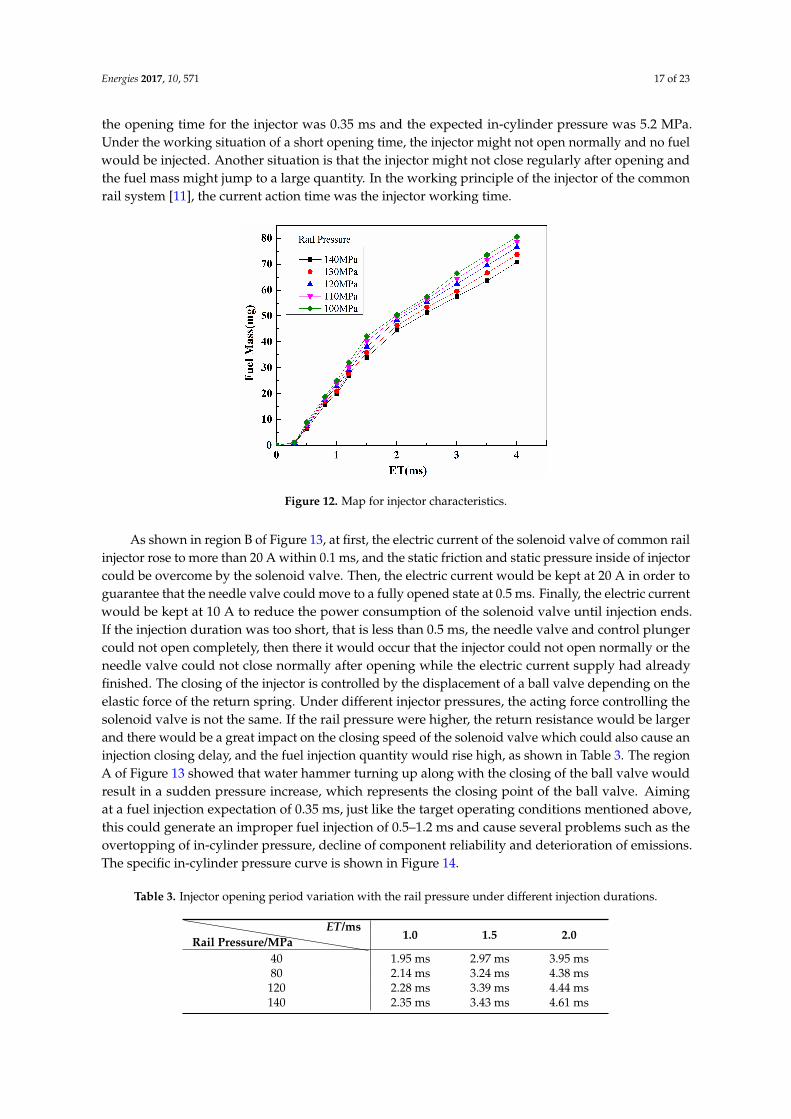
According to the working principles and operating requirements of the injector of a common railsystem, it can control the fuel injection quantity by using a time-pressure control method. That is, bylooking up the injection characteristics curve on the basis of the current rail pressure and target fuelquantity to obtain an injection duration ET and to control the cycle injection quantity. The injectioncharacteristics curve shown in Figure 12 was obtained from the test bench shown in Figure 1. Duringthe experiment, the first step was to adjust the rail pressure to the test value (100–140 MPa) by usingthe control system. After that, the injection period should be set to a constant (0.5–3.5 ms). By recordingthe fuel injection quantities 100 times with the single-injection instrument and taking an average, theinjection characteristics curve could be obtained. The operating features of the injector of the commonrail system are shown in Figure 12. When the rail pressure was 140 MPa, the minimum stable injectionduration was 0.5 ms and minimum fuel mass was 9 mg. When the calculated fuel mass equaled 6.5 mg,

Energies 2017, 10, 571 17 of 23

the opening time for the injector was 0.35 ms and the expected in-cylinder pressure was 5.2 MPa.Under the working situation of a short opening time, the injector might not open normally and no fuelwould be injected. Another situation is that the injector might not close regularly after opening andthe fuel mass might jump to a large quantity. In the working principle of the injector of the commonrail system [11], the current action time was the injector working time.

Energies 2017, 10, 571 17 of 23

in-cylinder pressure was 5.2 MPa. Under the working situation of a short opening time, the injector might not open normally and no fuel would be injected. Another situation is that the injector might not close regularly after opening and the fuel mass might jump to a large quantity. In the working principle of the injector of the common rail system [11], the current action time was the injector working time.

Figure 12. Map for injector characteristics.

As shown in region B of Figure 13, at first, the electric current of the solenoid valve of common rail injector rose to more than 20 A within 0.1 ms, and the static friction and static pressure inside of injector could be overcome by the solenoid valve. Then, the electric current would be kept at 20 A in order to guarantee that the needle valve could move to a fully opened state at 0.5 ms. Finally, the electric current would be kept at 10 A to reduce the power consumption of the solenoid valve until injection ends. If the injection duration was too short, that is less than 0.5 ms, the needle valve and control plunger could not open completely, then there it would occur that the injector could not open normally or the needle valve could not close normally after opening while the electric current supply had already finished. The closing of the injector is controlled by the displacement of a ball valve depending on the elastic force of the return spring. Under different injector pressures, the acting force controlling the solenoid valve is not the same. If the rail pressure were higher, the return resistance would be larger and there would be a great impact on the closing speed of the solenoid valve which could also cause an injection closing delay, and the fuel injection quantity would rise high, as shown in Table 3. The region A of Figure 13 showed that water hammer turning up along with the closing of the ball valve would result in a sudden pressure increase, which represents the closing point of the ball valve. Aiming at a fuel injection expectation of 0.35 ms, just like the target operating conditions mentioned above, this could generate an improper fuel injection of 0.5–1.2 ms and cause several problems such as the overtopping of in-cylinder pressure, decline of component reliability and deterioration of emissions. The specific in-cylinder pressure curve is shown in Figure 14.

Table 3. Injector opening period variation with the rail pressure under different injection durations.

ET/ms Rail Pressure/MPa

1.0 1.5 2.0

40 1.95 ms 2.97 ms 3.95 ms 80 2.14 ms 3.24 ms 4.38 ms

120 2.28 ms 3.39 ms 4.44 ms 140 2.35 ms 3.43 ms 4.61 ms

Figure 12. Map for injector characteristics.

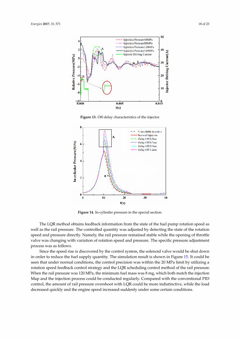
As shown in region B of Figure 13, at first, the electric current of the solenoid valve of common railinjector rose to more than 20 A within 0.1 ms, and the static friction and static pressure inside of injectorcould be overcome by the solenoid valve. Then, the electric current would be kept at 20 A in order toguarantee that the needle valve could move to a fully opened state at 0.5 ms. Finally, the electric currentwould be kept at 10 A to reduce the power consumption of the solenoid valve until injection ends.If the injection duration was too short, that is less than 0.5 ms, the needle valve and control plungercould not open completely, then there it would occur that the injector could not open normally or theneedle valve could not close normally after opening while the electric current supply had alreadyfinished. The closing of the injector is controlled by the displacement of a ball valve depending on theelastic force of the return spring. Under different injector pressures, the acting force controlling thesolenoid valve is not the same. If the rail pressure were higher, the return resistance would be largerand there would be a great impact on the closing speed of the solenoid valve which could also cause aninjection closing delay, and the fuel injection quantity would rise high, as shown in Table 3. The regionA of Figure 13 showed that water hammer turning up along with the closing of the ball valve wouldresult in a sudden pressure increase, which represents the closing point of the ball valve. Aimingat a fuel injection expectation of 0.35 ms, just like the target operating conditions mentioned above,this could generate an improper fuel injection of 0.5–1.2 ms and cause several problems such as theovertopping of in-cylinder pressure, decline of component reliability and deterioration of emissions.The specific in-cylinder pressure curve is shown in Figure 14.

Table 3. Injector opening period variation with the rail pressure under different injection durations.

Rail Pressure/MPaET/ms

1.0 1.5 2.0

40 1.95 ms 2.97 ms 3.95 ms80 2.14 ms 3.24 ms 4.38 ms120 2.28 ms 3.39 ms 4.44 ms140 2.35 ms 3.43 ms 4.61 ms


Figure 13. Off-delay characteristics of the injector.

Figure 14. In-cylinder pressure in the special section.

The LQR method obtains feedback information from the state of the fuel pump rotation speed as well as the rail pressure. The controlled quantity was adjusted by detecting the state of the rotation speed and pressure directly. Namely, the rail pressure remained stable while the opening of throttle valve was changing with variation of rotation speed and pressure. The specific pressure adjustment process was as follows.

Since the speed rise is discovered by the control system, the solenoid valve would be shut down in order to reduce the fuel supply quantity. The simulation result is shown in Figure 15. It could be seen that under normal conditions, the control precision was within the 20 MPa limit by utilizing a rotation speed feedback control strategy and the LQR scheduling control method of the rail pressure. When the rail pressure was 120 MPa, the minimum fuel mass was 8 mg, which both match the injection Map and the injection process could be conducted regularly. Compared with the conventional PID control, the amount of rail pressure overshoot with LQR could be more indistinctive, while the load decreased quickly and the engine speed increased suddenly under some certain conditions.


Energies 2017, 10, 571 18 of 23



The LQR method obtains feedback information from the state of the fuel pump rotation speed as well as the rail pressure. The controlled quantity was adjusted by detecting the state of the rotation speed and pressure directly. Namely, the rail pressure remained stable while the opening of throttle valve was changing with variation of rotation speed and pressure. The specific pressure adjustment process was as follows.

Since the speed rise is discovered by the control system, the solenoid valve would be shut down in order to reduce the fuel supply quantity. The simulation result is shown in Figure 15. It could be seen that under normal conditions, the control precision was within the 20 MPa limit by utilizing a rotation speed feedback control strategy and the LQR scheduling control method of the rail pressure. When the rail pressure was 120 MPa, the minimum fuel mass was 8 mg, which both match the injection Map and the injection process could be conducted regularly. Compared with the conventional PID control, the amount of rail pressure overshoot with LQR could be more indistinctive, while the load decreased quickly and the engine speed increased suddenly under some certain conditions.


The LQR method obtains feedback information from the state of the fuel pump rotation speed aswell as the rail pressure. The controlled quantity was adjusted by detecting the state of the rotationspeed and pressure directly. Namely, the rail pressure remained stable while the opening of throttlevalve was changing with variation of rotation speed and pressure. The specific pressure adjustmentprocess was as follows.

Since the speed rise is discovered by the control system, the solenoid valve would be shut downin order to reduce the fuel supply quantity. The simulation result is shown in Figure 15. It could beseen that under normal conditions, the control precision was within the 20 MPa limit by utilizing arotation speed feedback control strategy and the LQR scheduling control method of the rail pressure.When the rail pressure was 120 MPa, the minimum fuel mass was 8 mg, which both match the injectionMap and the injection process could be conducted regularly. Compared with the conventional PIDcontrol, the amount of rail pressure overshoot with LQR could be more indistinctive, while the loaddecreased quickly and the engine speed increased suddenly under some certain conditions.


Figure 15. Rail pressure, engine speed and fuel mass vs. time controlled by LQR.

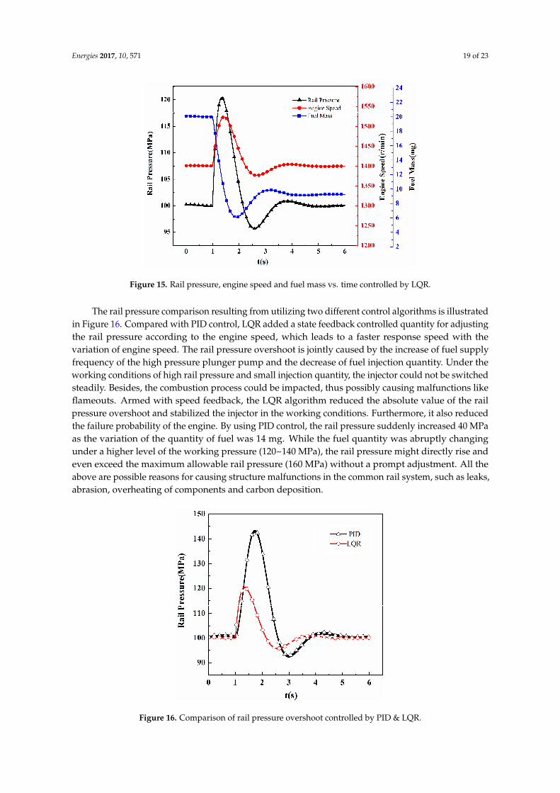
The rail pressure comparison resulting from utilizing two different control algorithms is illustrated in Figure 16. Compared with PID control, LQR added a state feedback controlled quantity for adjusting the rail pressure according to the engine speed, which leads to a faster response speed with the variation of engine speed. The rail pressure overshoot is jointly caused by the increase of fuel supply frequency of the high pressure plunger pump and the decrease of fuel injection quantity. Under the working conditions of high rail pressure and small injection quantity, the injector could not be switched steadily. Besides, the combustion process could be impacted, thus possibly causing malfunctions like flameouts. Armed with speed feedback, the LQR algorithm reduced the absolute value of the rail pressure overshoot and stabilized the injector in the working conditions. Furthermore, it also reduced the failure probability of the engine. By using PID control, the rail pressure suddenly increased 40 MPa as the variation of the quantity of fuel was 14 mg. While the fuel quantity was abruptly changing under a higher level of the working pressure (120~140 MPa), the rail pressure might directly rise and even exceed the maximum allowable rail pressure (160 MPa) without a prompt adjustment. All the above are possible reasons for causing structure malfunctions in the common rail system, such as leaks, abrasion, overheating of components and carbon deposition.

Figure 16. Comparison of rail pressure overshoot controlled by PID & LQR.


The rail pressure comparison resulting from utilizing two different control algorithms is illustratedin Figure 16. Compared with PID control, LQR added a state feedback controlled quantity for adjustingthe rail pressure according to the engine speed, which leads to a faster response speed with thevariation of engine speed. The rail pressure overshoot is jointly caused by the increase of fuel supplyfrequency of the high pressure plunger pump and the decrease of fuel injection quantity. Under theworking conditions of high rail pressure and small injection quantity, the injector could not be switchedsteadily. Besides, the combustion process could be impacted, thus possibly causing malfunctions likeflameouts. Armed with speed feedback, the LQR algorithm reduced the absolute value of the railpressure overshoot and stabilized the injector in the working conditions. Furthermore, it also reducedthe failure probability of the engine. By using PID control, the rail pressure suddenly increased 40 MPaas the variation of the quantity of fuel was 14 mg. While the fuel quantity was abruptly changingunder a higher level of the working pressure (120~140 MPa), the rail pressure might directly rise andeven exceed the maximum allowable rail pressure (160 MPa) without a prompt adjustment. All theabove are possible reasons for causing structure malfunctions in the common rail system, such as leaks,abrasion, overheating of components and carbon deposition.

Energies 2017, 10, 571 19 of 23


The rail pressure comparison resulting from utilizing two different control algorithms is illustrated in Figure 16. Compared with PID control, LQR added a state feedback controlled quantity for adjusting the rail pressure according to the engine speed, which leads to a faster response speed with the variation of engine speed. The rail pressure overshoot is jointly caused by the increase of fuel supply frequency of the high pressure plunger pump and the decrease of fuel injection quantity. Under the working conditions of high rail pressure and small injection quantity, the injector could not be switched steadily. Besides, the combustion process could be impacted, thus possibly causing malfunctions like flameouts. Armed with speed feedback, the LQR algorithm reduced the absolute value of the rail pressure overshoot and stabilized the injector in the working conditions. Furthermore, it also reduced the failure probability of the engine. By using PID control, the rail pressure suddenly increased 40 MPa as the variation of the quantity of fuel was 14 mg. While the fuel quantity was abruptly changing under a higher level of the working pressure (120~140 MPa), the rail pressure might directly rise and even exceed the maximum allowable rail pressure (160 MPa) without a prompt adjustment. All the above are possible reasons for causing structure malfunctions in the common rail system, such as leaks, abrasion, overheating of components and carbon deposition.

Figure 16. Comparison of rail pressure overshoot controlled by PID & LQR. Figure 16. Comparison of rail pressure overshoot controlled by PID & LQR.

Energies 2017, 10, 571 20 of 23

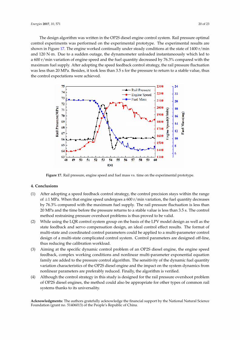
The design algorithm was written in the OP2S diesel engine control system. Rail pressure optimalcontrol experiments was performed on the experimental prototype. The experimental results areshown in Figure 17. The engine worked continually under steady conditions at the state of 1400 r/minand 120 N·m. Due to a sudden outage, the dynamometer unloaded instantaneously which led toa 600 r/min variation of engine speed and the fuel quantity decreased by 76.3% compared with themaximum fuel supply. After adopting the speed feedback control strategy, the rail pressure fluctuationwas less than 20 MPa. Besides, it took less than 3.5 s for the pressure to return to a stable value, thusthe control expectations were achieved.

Energies 2017, 10, 571 20 of 23

The design algorithm was written in the OP2S diesel engine control system. Rail pressure optimal control experiments was performed on the experimental prototype. The experimental results are shown in Figure 17. The engine worked continually under steady conditions at the state of 1400 r/min and 120 N·m. Due to a sudden outage, the dynamometer unloaded instantaneously which led to a 600 r/min variation of engine speed and the fuel quantity decreased by 76.3% compared with the maximum fuel supply. After adopting the speed feedback control strategy, the rail pressure fluctuation was less than 20 MPa. Besides, it took less than 3.5 s for the pressure to return to a stable value, thus the control expectations were achieved.

Figure 17. Rail pressure, engine speed and fuel mass vs. time on the experimental prototype.

4. Conclusions

(1) After adopting a speed feedback control strategy, the control precision stays within the range of ±1 MPa. When that engine speed undergoes a 600 r/min variation, the fuel quantity decreases by 76.3% compared with the maximum fuel supply. The rail pressure fluctuation is less than 20 MPa and the time before the pressure returns to a stable value is less than 3.5 s. The control method restraining pressure overshoot problems is thus proved to be valid.

(2) While using the LQR control system group on the basis of the LPV model design as well as the state feedback and servo compensation design, an ideal control effect results. The format of multi-state and coordinated control parameters could be applied to a multi-parameter control design of a multi-state complicated control system. Control parameters are designed off-line, thus reducing the calibration workload.

(3) Aiming at the specific dynamic control problem of an OP2S diesel engine, the engine speed feedback, complex working conditions and nonlinear multi-parameter exponential equation family are added to the pressure control algorithm. The sensitivity of the dynamic fuel quantity variation characteristics of the OP2S diesel engine and the impact on the system dynamics from nonlinear parameters are preferably reduced. Finally, the algorithm is verified.

(4) Although the control strategy in this study is designed for the rail pressure overshoot problem of OP2S diesel engines, the method could also be appropriate for other types of common rail systems thanks to its universality.

Acknowledgments: The authors gratefully acknowledge the financial support by the National Natural Science Foundation (grant no. 51406013) of the People’s Republic of China.

Author Contributions: Yi Lu and Changlu Zhao designed the simulation scheme; Yi Lu and Zhe Zuo performed the simulations; Zhe Zuo and Shuanlu Zhang analyzed the data; Yi Lu and Fujun Zhang contributed to the editing and reviewing of the document.

Figure 17. Rail pressure, engine speed and fuel mass vs. time on the experimental prototype.

4. Conclusions

(1) After adopting a speed feedback control strategy, the control precision stays within the rangeof ±1 MPa. When that engine speed undergoes a 600 r/min variation, the fuel quantity decreasesby 76.3% compared with the maximum fuel supply. The rail pressure fluctuation is less than20 MPa and the time before the pressure returns to a stable value is less than 3.5 s. The controlmethod restraining pressure overshoot problems is thus proved to be valid.

(2) While using the LQR control system group on the basis of the LPV model design as well as thestate feedback and servo compensation design, an ideal control effect results. The format ofmulti-state and coordinated control parameters could be applied to a multi-parameter controldesign of a multi-state complicated control system. Control parameters are designed off-line,thus reducing the calibration workload.

(3) Aiming at the specific dynamic control problem of an OP2S diesel engine, the engine speedfeedback, complex working conditions and nonlinear multi-parameter exponential equationfamily are added to the pressure control algorithm. The sensitivity of the dynamic fuel quantityvariation characteristics of the OP2S diesel engine and the impact on the system dynamics fromnonlinear parameters are preferably reduced. Finally, the algorithm is verified.

(4) Although the control strategy in this study is designed for the rail pressure overshoot problemof OP2S diesel engines, the method could also be appropriate for other types of common railsystems thanks to its universality.

Acknowledgments: The authors gratefully acknowledge the financial support by the National Natural ScienceFoundation (grant no. 51406013) of the People’s Republic of China.

Energies 2017, 10, 571 21 of 23

Author Contributions: Yi Lu and Changlu Zhao designed the simulation scheme; Yi Lu and Zhe Zuo performedthe simulations; Zhe Zuo and Shuanlu Zhang analyzed the data; Yi Lu and Fujun Zhang contributed to the editingand reviewing of the document.

Conflicts of Interest: The authors declare no conflict of interest.

Nomenclature

AbbreviationBDC Bottom Dead CenterECU Electronic Control UnitLPV Linear Parameter VaryingLQR Linear Quadratic RegulatorOP2S Opposed-Piston Two-StrokePCV Pressure Control ValvesPWM Pulse Width ModulationPID Proportion Integration DifferentiationSymbolsα Crank angle, degρ Fuel density, kg/m3

a Correction coefficientb Correction coefficientc Discharge coefficientET Injection pulse widthJEngine Moment of inertia in engine, kg ·m2

k Injector numberKf Fuel bulk modulus of elasticity, MPaKT Model constantsKp Rail pressure state feedback parameterKn Speed state feedback parameterKe Servo compensation state feedback parametern Crankshaft speed, r/minp Time varying fuel pressure, MPapg Constant fuel pressure,0.5MPaq Fuel flow, m3/ssp Plunger instantaneous axial displacement, mTload Load torque, N ·mu Control signalsv Instantaneous fuel volume, m3

V Constant volume, m3

Subscripts0 Initial valuecyl cylinderi injectorin flow directionout flow directionp pumpr rails solenoid valve of pumpd desired rail pressure

References

1. Pirault, J.P.; Flint, M. Opposed Piston Engines: Evolution, Use, and Future Applications; SAE International:Warrendale, PA, USA, 2009.

2. Ma, F.; Zhao, C.; Zhang, F.; Zhao, Z.; Bingham, C. Effects of Scavenging System Configuration on In-CylinderAir Flow Organization of an Opposed-Piston Two-Stroke Engine. Energies 2015, 2015, 5866–5884. [CrossRef]

http://dx.doi.org/10.3390/en8065866

Energies 2017, 10, 571 22 of 23

3. Peter, H. Opposed Piston Opposed Cylinder (OPOC) Engine for Military Ground Vehicles; SAE Technical Paper2005-01-1548; SAE International: Warrendale, PA, USA, 2005.

4. Naik, S.; Johnson, D.; Koszewnik, J.; Fromm, L.; Redon, F.; Regner, G.; Fuqua, K. Practical Applications ofOpposed-Piston Engine Technology to Reduce Fuel Consumption and Emissions; SAE Technical Paper 2013-01-2754;SAE International: Warrendale, PA, USA, 2013.

5. Regner, G.; Johnson, D.; Koszewnik, J.; Lynn, F. Modernizing the Opposed Piston, Two Stroke Engine for Clean,Efficient Transportation; SAE Technical Paper 2013-26-0114; SAE International: Warrendale, PA, USA, 2013.

6. Gharakhani, A.; Ghoniem, A.F. 3D vortex simulation of flow in an opposed-piston engine. Esaim Proc. 1999,7, 161–172. [CrossRef]

7. Regner, G.; Herold, R.E.; Wahl, M.H.; Dion, E.; Redon, F.; Johnson, D.; McIntyre, S. The Achates PowerOpposed-Piston Two-Stroke Engine: Performance and Emissions Results in a Medium-Duty Application; SAETechnical Paper 2011-01-2221; SAE International: Warrendale, PA, USA, 2011.

8. Stumpp, G.; Ricco, M. Common Rail-An Attractive Fuel Injection System for Passenger Car DI Diesel Engines.In Proceedings of the International Congress and Exposition of the Society of Automotive Engineers (SAE),Detroit, MI, USA, 26–29 February 1996.

9. Boehner, W.; Hummel, K. Common Rail Injection System for Commercial Diesel Vehicles; SAE International:Warrendale, PA, USA, 1997.

10. Catania, A.E.; Ferrari, A.; Manno, M.; Spessa, E. Experimental Investigation of Dynamic Effects onMultiple-Injection Common Rail System Performance. J. Eng. Gas Turbines Power 2008, 130, 460–466.[CrossRef]

11. Henein, N.A.; Lai, M.C.; Singh, I.P.; Zhong, L.; Han, J. Characteristics of a Common Rail Diesel Injection Systemunder Pilot and Postinjection Modes; SAE Technical Paper 2002-01-0218; SAE International: Warrendale, PA,USA, 2002.

12. Bianchi, G.M.; Falfari, S.; Pelloni, P.; Filicori, F.; Milani, M.A. Numerical and Experimental Study towards PossibleImprovements of Common Rail Injectors; SAE Technical Paper 2002-01-0500; SAE International: Warrendale, PA,USA, 2002.

13. Yang, F.Y.; Zhang, J.Y.; Wang, X.G.; Zhou, M.; Ouyang, M.G. Judgement and Application of Ignition Momentduring Engine Startup Period Based on Crankshaft Transient Acceleration Analysis. Autom. Eng. 2003, 25,111–115.

14. Song, G.M.; Yang, F.Y.; Ouyang, M.G.; Hu, L.F.; Hang, Y. Equilibrium Algorithm Research for Each IndividualCylinders of Common Rail Based on Self-Adaptive Fuzzy Control. Trans. Csice 2005, 23, 451–456.

15. Song, J.; Tian, L.Y.; Li, X.L.; Qiao, X.Q.; Huang, Z. Design of ECU for Common Rail System of Diesel Engineand Study of Injection Characteristics. Trans. Csice 2006, 24, 28–34.

16. Xu, J.; Shen, L.Z.; Wang, G.; Bi, Y. Study on Compound Control Strategy of Rail Pressure for High PressureCommon Rail Diesel Engine. Chin. Intern. Combust. Engine Eng. 2012, 33, 54–59.

17. Zhou, W.H.; Zhu, C.D.; Yu, S.U. Key technology of electronic controlled system of common-rail diesel engine.J. Zhejiang Univ. 2011, 45, 118–121.

18. Li, S.; Chen, H.; Ma, M. Model predictive control based on linear programming for engine idle speedcontrol. In Proceedings of the IEEE Conference on Mechatronics and Automation (ICMA), Changchun,China, 9–12 August 2009.

19. Li, S.; Chen, H.; Yu, S. Nonlinear model predictive control for idle speed control of SI engine. In Proceedingsof the IEEE Conference on Decision and Control Jointly with the, Chinese Control Conference, Shanghai,China, 16–18 December 2009.

20. Fialho, I.; Balas, G.J. Road adaptive active suspension design using linear parameter-varying gain-scheduling.IEEE Trans. Control Syst. Technol. 2002, 10, 43–54. [CrossRef]

21. Kjergaard, L.; Nielsen, S.; Vesterholm, T.; Hendricks, E. Advanced Nonlinear Engine Idle Speed ControlSystems. In Proceedings of the International congress and exposition of the Society of Automotive Engineers(SAE), Detroit, MI, USA, 26–29 March 1994.

22. Yu, S.T.; Zhou, X.L.; Yang, X.F.; Gong, Y.M.; Yang, L.; Zhou, B. Research on torque based control simulationmodel for electronic unit pump diesel engine. Chin. Intern. Combust. Engine Eng. 2006, 27, 29–32.

23. Lino, P.; Maione, B.; Rizzo, A. Nonlinear modeling and control of a common rail injection system for dieselengines. Appl. Math. Model. 2007, 31, 1770–1784. [CrossRef]

http://dx.doi.org/10.1051/proc:1999015

http://dx.doi.org/10.1115/1.2835353

http://dx.doi.org/10.1109/87.974337

http://dx.doi.org/10.1016/j.apm.2006.06.001

Energies 2017, 10, 571 23 of 23

24. Lino, P.; Maione, B.; Amorese, C. Modelling and predictive control of a new injection system for compressednatural gas engines. Control Eng. Pract. 2006, 16, 1216–1230. [CrossRef]

25. Catania, A.E.; Ferrari, A.; Manno, M. Development and Application of a Complete Common-Rail InjectionSystem Mathematical Model for Hydrodynamics Analysis and Diagnostics. In Proceedings of the ASMEICE Spring Technical Conference, Chicago, IL, USA, 5–7 April 2005.

26. Di Gaeta, A.; Palladino, G.F.A.; Giglio, V. A control oriented model of a Common-Rail System for GasolineDirect Injection Engine. In Proceedings of the IEEE Conference on Decision and Control jointly with theChinese Control Conference, Shanghai, China, 16–18 December 2009.

27. Di Gaeta, A.; Fiengo, G.; Palladino, A.; Giglio, V. Design and Experimental Validation of a Model-BasedInjection Pressure Controller in a Common Rail System for GDI Engine. In Proceedings of the AmericanControl Conference, San Francisco, CA, USA, 29 June–1 July 2011.

28. Wei, X.; del Re, L. Gain Scheduled H Control for Air Path Systems of Diesel Engines Using LPV Techniques.IEEE Trans. Control Syst. Technol. 2007, 15, 406. [CrossRef]

29. Salcedo, J.; Martínez, M. LPV identification of a turbocharged diesel engine. Appl. Numer. Math. 2008, 58,1553–1571. [CrossRef]

30. White, A.P.; Zhu, G.; Choi, J. Gain-scheduling control of port-fuel-injection processes. Control Eng. Pract.2011, 19, 380–394. [CrossRef]

31. Bullock, D.; Johnson, B.; Wells, R.B.; Kyte, M.; Li, Z. Hardware-in-the-loop simulation. Transp. Res. Part CEmerg. Technol. 2004, 12, 73–89. [CrossRef]

32. Heemels, W.P.M.H.; Daafouz, J.; Millerioux, G. Observer-based control of discrete-time LPV systems withuncertain parameters. IEEE Trans. Autom. Control 2010, 55, 2130–2135. [CrossRef]

33. White, A.; Zhu, G.; Choi, J. Optimal LPV control with hard constraints. Int. J. Control Autom. Syst. 2016, 14,148–162. [CrossRef]

34. GT-Power User’s Manual Version 6.2[M]; Gamma Technologies: Westmont, IL, USA, 2006.35. Ciesla, C.; Keribar, R.; Morel, T. Engine/Powertrain/Vehicle Modeling Tool Applicable to All Stages of the Design

Process; SAE Technical Paper 2000-01-0934; SAE International: Warrendale, PA, USA, 2000.36. Morel, T.; Keribar, R.; Leonard, A. Virtual Engine/Powertrain/Vehicle Simulation Tool Solves Complex Interacting

System Issues; SAE Technical Paper 2003-01-0372; SAE International: Warrendale, PA, USA, 2003.

© 2017 by the authors. Licensee MDPI, Basel, Switzerland. This article is an open accessarticle distributed under the terms and conditions of the Creative Commons Attribution(CC BY) license (http://creativecommons.org/licenses/by/4.0/).

http://dx.doi.org/10.1016/j.conengprac.2008.01.008

http://dx.doi.org/10.1109/TCST.2007.894633

http://dx.doi.org/10.1016/j.apnum.2007.09.005

http://dx.doi.org/10.1016/j.conengprac.2010.12.007

http://dx.doi.org/10.1016/j.trc.2002.10.002

http://dx.doi.org/10.1109/TAC.2010.2051072

http://dx.doi.org/10.1007/s12555-014-0248-4

http://creativecommons.org/

http://creativecommons.org/licenses/by/4.0/.

Documents

Research on the Common Rail Pressure Overshoot of Opposed ...€¦ · energies Article Research on the Common Rail Pressure Overshoot of Opposed-Piston Two-Stroke Diesel Engines Yi