Research Paper - Dallasfed.org/media/documents/research/papers/1992/... · Research Paper Federal Reserve Bank ... of the initial orthodox adjustment and acceleration of inflation,

No. 9210

COINTEGRATION AND TESTS OF A CLASSICAL HODELOFINFLATION IN ARGENTINA, BOLIVIA,

BRAZIL, MEXICO. AND PERU

by

Raul Anibal Feliz and John H. Welch

June 1992

Research Paper

Federal Reserve Bank. of Dallas

This publication was digitized and made available by the Federal Reserve Bank of Dallas' Historical Library ([email protected])

Cointegration and Tests of a Classical Model of Inflation in

Argentina, Bolivia, Brazil, Mexico, and Peru

July 1992Preliminary. Comments welcomed.

Raul Anibal FelizDivisi6n de Economia

Centro de Investigaci6n y Docencia EconomicasCarrretera Mexico-Toluca KIn. 16.5

Lomas de Santa Fe01210 Mexico D.F

Tel. 259-1210 ext. 222, Fax 570-4277

John H. WelchSenior Economist

Federal Reserve Bank of DallasResearch Department, Station K, Dallas, TX 75222,

Tel. (214)922-5165, Fax. (214)922-5194.

We would like to thank Shengyi Guo for excellent research assistance. We would also liketo thank without implicating Joe Haslag for his comments on an earlier draft of the paper.Any errors and omissions as well as any opinion, propositions, or conclusions are exclusivelyour own. The contents reflect the authors' own views and should not be associated with theFederal Reserve Bank of Dallas nor with the Federal Reserve System.

Abstract

The failure of the "heterodox" inflation stabilization attempts of the 1980s in Argentina,Brazil and Peru along with the apparent success of the more orthodox Bolivian and Mexicanstabilizations have left researchers again looking at the dynamics of inflation. This paperseeks to add to recent findings by testing whether the recent seemingly different inflationexperiences in Argentina, Bolivia, Brazil, Mexico and Peru are consistent with the newclassical model-of'-inflation. -Monetary modelsofinflation with rational expectations carrya number of testable implications. First, money growth and inflation should be cointegratedwhile the short term dynamics display temporary and stochastic dislocations from thisequilibrium relationship. Second, the equilibrium error anticipates future monetary policydue the fact that agents have superior information to that of the econometrician. Third,cointegration between money growth and inflation implies, as Campbell and Shiller (1987and 1988) show, that cross equation restrictions can be readily generated from the errorcorrection form. Our results show that the new classical model of inflation is generallyconsistent with the inflation experiences of Argentina, Bolivia, Brazil, Mexico, and Peru inspite of their supposed heterogeneity.

Introduction

The inflationary process in Latin America has received a large amount of attention

over the last decade especially after the onset of the debt crisis in 1982. In the aftermath

of the initial orthodox adjustment and acceleration of inflation, a strong revisionist version

of the old monetarist-structuralist debate emerged.' The older monetarist inflation theories

have been supplanted by rational expectations models of inflation while structuralist theories

grew into new-structuralist or "inertial" inflation theories. The failure of the "heterodox"

inflation stabilization attempts of the 1980s in Argentina, Brazil, and Peru along with the

apparent success of the more orthodox Bolivian and Mexican stabilizations have left

researchers again looking at the dynamics of inflation. This paper seeks to add to recent

findings by testing whether the recent inflation experiences in Argentina, Bolivia, Brazil,

Mexico and Peru are consistent with the new classical model of inflation.

The inflation experiences of these countries differed in the 1980s (Figures 1 - 5).'

Four of the countries attempted "heterodox" stabilization policies combining incomes policies

-with monetary and fiscal austerity: Argentina in 1985-1987, 1988, and 1989, Brazil in 1986,

1987, 1989, and 1990, Mexico in the period 1988 to the present, and Peru in 1986-1987. Only

ISee the articles in Baer and Welch (1987) for discussions of the initial adjustment whichignited the revised monetarist-structuralist debate. Sargent (1986) succinctly lays out thenew classical view of inflation. The works contained in Baer and Kerstenetzky (1964)present a good summary of the old debate.

'Good reviews on the recent inflation experiences in each of these countries includeBruno, et ai, (1991), Pastor (1989), Sachs and Morales (1988), Paredes and Sachs (1991),and Dornbusch and Edwards (1991).

1

the Mexican program proved a long term success. Four of the countries's inflation rates

reached hyperinflationary levels: Argentina in June and July 1989 and December 1989,

Bolivia in early 1985, Brazil in 1990, and Peru in 1990-1991. Only two of these countries

had brought their inflation rates back to moderate levels by 1990, Bolivia and Mexico. The

sample of countries used in this study offers a rich diversity of high inflation experiences in

1980s. The aim of this paper is to see if the classical model successfully describes the

inflationary process across these experiences.

Monetary models of inflation with rational expectations carry a number of testable

implications. First, the main tenet of monetary models is that inflation is (ultimately) a

monetary phenomenon. This precludes the existence of speculative sources of inflation. In

the context of rational expectations, speculative bubbles can theoretically emerge due the

inconsistency inherent in models where the present price level is a function of future

expected price levels [Diba and Grossman 1988a and 1988b]. Theoretically, inflation can

accelerate infinitely even though money grow remains stationary. Such bubbles, however,

would have the growth rates of prices and money continuously diverging which precludes

'cointegration between inflation and money growth. Hence, one can empirically rule out

inflationary bubbles if money growth and inflation are cointegrated. We will interpret the

non-existence of rational inflation bubbles to mean that the inflationary process is consistent

with monetary models in general.

Second, forward looking or rational expectations imply structural restrictions on the

monetary model which can be interpreted best in the context of cointegrated models. The

solution for the inflation rate in these models resembles the general form for the present

2

value models of Campbell and Shiller (1987 and 1988). Specifically, the models imply that

money growth and inflation are cointegrated in the long run while the short term dynamics

display temporary and stochastic dislocations from this equilibrium relationship. These

"disequilibria", however, in turn do not imply that the present value model is not valid. On

the contrary, the equilibrium error can be seen to anticipate future monetary policy due the

fact that agents have superior information than does the econometrician. Causality running

from the equilibrium error to money growth and inflation does not imply that the error

causes changes in the variables of the model but instead anticipates them [Campbell and

Shiller 1988: 506-507).

Cointegration between money growth and inflation, given the above interpretation,

suggests that the appropriate framework should be an error correction representation for

the two joint processes. As Campbell and Shiller (1987 and 1988) show, the cross equation

restrictions can be readily generated from the error correction form. Unfortunately,

rejection of these cross equation restrictions, however, does not lead to any clear

interpretation of the underlying inflation-money growth dynamic. The ultimate goal of the

-analysis is to gauge the ability of the model to describe the inflationary process in each of

these countries.

The paper is organized as follows. Section I presents a model of inflation in line the

with classical theory and discusses the stationarity properties of money growth and inflation.

Cross equation restrictions are developed in section II. The empirical results of the model

are shown in section III while section IV summarizes and concludes the paper.

3

I. A Classical Model of Inflation

The model starts with the money demand specification of Cagan (1956).

m, - P, = Y, - a.i, + E, (1)

where m, is the natural logarithm of the money stock, p, is the natural logarithm of the price

level, y, is the natural logarithm of real output, i, is the nominal interest rate, and e, is a zero

mean random error term all evaluated at time to' The standard assumption describes E, as

a random walk of the form

(2)

where I), is white noise.

The classical model assumes a Fisher relationship for the nominal interest rate.

(3)

where r, is the real interest rate, E["] is the expectations operator, 1T,,, = p,+. - p, is the

logarithmic inflation rate, and <P, is the information set at time 1. The model subsumes

rational expectations, i.e. individuals use all information available to them to form

expectations about future inflation rates.

'This error term can be viewed as one which is either viewed by market participants orconstructed by them. E" however, is not observed by the researcher. See Diba andGrossman (1988a) and Campbell and Shiller (1987 and 1988).

4

Real output and real interest rates are assumed to follow random walks (real output

also has a drift).

where c.>1t and c.>~ are white noise.

Y -y =y-+c.>,,-1 It(4)

(5)

Taking first differences on equation (1) and combined with equations (2) to (5) yields

the following expression.

(6)

where IJ., is the logarithmic growth of money and

(7)

is white noise.

Rearranging equation (6) yields

(8)

Taking expectations on equation (8) conditional on <P,., and solving forward n periods

into the future into equation (9) yields

5

(9)

For the evolution of inflation expectations (and thus inflation) to be stable (no

bubbles), they must satisfy the following transversality condition

(10)

If equation (10) is satisfied, the no bubbles solution to the inflation rate is

(11)

On the other hand, if the transversality condition is violated, a rational bubble can

exist. For the bubble to be consistent with expectations, it must evolve in the following way

Solutions to (14) satisfy the stochastic difference equation

(1 + a)

B'+1 - a B. = "+1

6

(12)

(13)

where the random variable C, satisfies

The solution of-inflation rate ·with a bubble is'

(14)

The presence of bubbles carries a number of implications [Diba and Grossman

1988a: 522-523]. The first is that the presence of bubbles precludes the stationarity of any

degree of differencing of the inflation series. Taking first differences of the bubble in

equation (16) using the lag operator L yields'

(16)

One could continue differencing this representation of the bubble. The ARMA

representation of equation (20), however, will never be stationary (as the root of [1-

«1 +a)/a)z] = 0 lies inside the unit circle) nor invertible. The bubble introduces a non-

'To see this note that

1E[B,.!I ~ ,-1] - B, = -B,

Ct.

Substituting this value into equation (8) yields the additive term B,.

'The following discussion follows Diba and Grossman's (1988a and 1988b).

7

stationarity which cannot be differenced away.

The presence of bubbles would also rule out cointegration between inflation and

money growth. Reconsider equation (19) which /aates

1'1:, = IJ., - j +

Suppose both inflation and money growth are stationary after first differencing ( i.e.

integrated of order 1 or I( I» and recall that the growth rate of real output is assumed to

be constant. In this classical representation, the left hand side of equation (21) is an

equilibrium relationship of inflation and money growth with cointegrating vector a' = [I,

-1] and an intercept while the right hand represents the residuals Z,. If there are no

bubbles, the residuals are stationary and inflation and money growth are cointegrated of

order (1,1). In the presence of bubbles, however, the residuals of the cointegrating

regression are not stationary. Hence, if inflation and money growth are cointegrated, no

bubbles exist. Further, cointegration of money growth and inflation rules out any non

stationarity of the unobserved variables [Diba and Grossman 1988a: 525-526]. Hamilton and

Whiteman (1985) come to similar conclusions by showing that if money growth is stationary

after d differences and inflation is stationary after differencing d times, then speculative

inflationary bubbles cannot exist.

II Cross Equation Restrictions

The new classical view of inflation posits that inflation rates are functions of current

8

and expected future money growth rates. The form of these relationships generate a set of

easily testable restrictions on the inflationary process. The inflation generation process of

the classical model without bubbles followed

11:, = j.l, - j + (18)

The task now is to derive an error correction form of the monetary growth process in order

to generate forecasts of f.I-,+j and then test the restrictions implied by equation (1).

Suppose inflation and money growth are both 1(1) and cointegrated CI(I,I). The

trick now is to generate an error correction representation of the inflationary process. Let

the time series vector X, = [71'" f.I-,]. By the Wold decomposition theorem, X, can be

represented

(1 - L)X, = C(L)v, (19)

where C(L) is a 2 x 2 matrix in the lag operator and V, is a vector white noise process with

V, = [v"" v,,].

Engle and Granger (1987) show that the corresponding ARMA representation of the

MA process of equation (2) will not be invertible and that an error correction form would

be the appropriate model choice. To see this, multiply both sides of equation (2) by the

cointegrating vector [1, -1] to gel

9

(1-L)Z, = a'(1 - L)X, = a'C(L)v,

For Z, to be stationary, Le. 1(0),

a'C(1) = 0

(20)

(21)

where 0 is a 1 x 2 vector of zeros. Hence, C(L) = C(1) + (I-L)C'(L) cannot be simply

inverted to form an AR representation of x,. Granger and Engle (1987) show that the

CI(I,I) process of equation (2) will have an error correction representation'

(1 - L)X, = A *(L)(1 - L)X, - AZ'_l + b(L)vI (22)

where A'(O) = 0, A is a vector of constants, A is a (2 x 1) vector of constants, det[C(L») =

(I-L)b(L»), and beL) is a scaler lag polynomial. As beL) is invertible, premultiplying

equation (5) by b"(L) yields

D(L)(l - L)X, = -g(L)AZ/-l + v, (23)

where D(L) = b"(L)[I-A"(L») = b"(L)A(L) and geL) = b't(L). Define the matrix M as

"The Granger Representation Theorem [Engle and Granger 1987: 255-256]. Theseresults follow from factoring the adjoint matrix of C(L).

10

and

Now

MX, = [0 ~ ITt'] = [11,]1 1 11, Z,

x, = M-1[11,] = [1 11111]

Z, 1 0 Z,

Substituting equation (30) into equation (27) yields

(24)

(25)

(26)

(27)

Since (I-L) is a scaler in L, equation (10) can be rearranged in the following way"

'See Campbell and Shiller (1988), p. 510-511. The intuition behind this reformulationlies in the fact that Z, is stationary.

11

[

(1 - L)I-I,]Jf(L) = w,

Z,(28)

In order-to~enerate .optimal forecasts of -money growth, we rewrite the VAR

representation of equation (11) in the following way

Y, = 8YH + e,

where

(l-L)I-I,

(l-L)uH

o

(29)

(l-L)I-I,_p-l

(l-L)I-I,_p0 (30)y = e =, ,

Z,w2t

0Z'_l

o

12

and e is the companion matrix of the VAR of the form

6111 6112 61lp- 2 61lp 6121 6122 6121'_1 6121'

1 0 0 0 0 0 0 0

0 1 0 0 0 0 0 0

0 0 1 0 0 0 0 0 (31)e =6211 62\2 621P- 1 621p 6221 6= 6221'_1 6221'

0 0 0 0 1 0 0 0

0 0 0 0 0 1 0 0

o 0 o 000 1 o

Optimal forecasts of the Y, will thus be generated by

(32)

One important aspect of the VAR of equation (36) is that if the cointegrated present

value model holds, Z, will "Granger-cause" changes in money growth and changes in inflation

[Campbell and Shiller 1988: 513]. If economic agents have superior information to that of

the econometrician, one would find that the equilibrium error anticipates the changes in

inflation and money growth. Hence, below we test for such a causal relationship.

Equation (1) implies a set of restrictions on the optimal forecast equation (15).

13

Recall the money demand function

(33)

Rewritmg-equation (37) in the new notation yields

Taking expectations conditional on <P'_k of equation (38) and rearranging yields

_ 1 Y Iql ] = 01 + a .-k

(35)

Let R, = [0,0, ...,0,1,0,0,...,0,0] and R2 = [1,0,...,0,0,0,0, ...,0,0]. The classical restrictions

in equation (18) can be expressed as

which are non-linear in the parameter matrix e. The Wald statistic for this test is

oj( oHt)'. (OHt)]-1 ° 2THI -- 1:9 -- HI - Xpae ae

(36)

(37)

where T is the number of observations and k. is the estimated covariance matrix of the

14

estimated a matrix.

III Empirical Results

a. Cointegration Tests

Before moving to the tests for cointegration, tests on the order of integration are in

order.' Tables 1 through 10 show the Dickey-Fuller (1979) and Phillips-Perron (1988) tests

for stationarity for money and prices in Argentina, Bolivia, Brazil, Mexico, and Peru. The

Phillips and Perron (1988) tests correct for non-normality of variables (tested for using the

Jarque and Bera (1980) tests). In Argentina, Bolivia, Brazil, Mexico, and Peru, M, money

growth and inflation are strongly stationary after differencing. In all countries, inflation is

not unambiguously 1(1) as opposed to 1(0). The cointegration tests below, however, indicate

that it is I(1) as is money growth.'

Generally, cointegration means that (non-stationary) time series variables tend to

move together such that a linear combination of them is stationary. As in the analysis

above, some have interpreted cointegration as representing a long run equilibrium

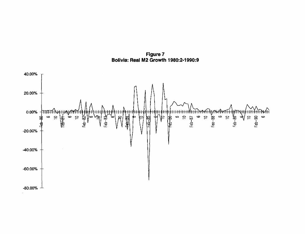
'Inflation in both countries is measured by the wholesale price index and M, was pickedas the monetary aggregate based upon cointegration tests on the money demand equation(1). The conclusions of the tests, however, do not depend on the choice of moneyaggregate. The Argentine data are quarterly observations from 1970 to 1984 and come fromINDEC. The Bolivian data are monthly observations from June 1980 to September 1990from the Banco Central de Bolivia. The Brazilian data are monthly observations from 1974to 1985 and come from the Funda"ao Getulio Vargas. The Mexican data are monthlyobservations from January 1972 to September 1989 from the Banco de Mexico IndicadoresEconomicos and from the data bank of Sie-Mexico. Finally, Peru's data are monthlyobservations from January 1983 to June 1990 from the Banco Central de Peru.

'M, was use<Uis.the money aggregate.in.all countries except Mexico. We used M, forMexico but the results hold for M, as well.

15

relationship. Differencing X, d times to generate a stationary time senes and then

estimating a VAR based upon the differenced series is inappropriate in the presence of

cointegration. Recall that if a (pxl) vector time series X, (p=2 in this case) is first

difference stationary, i.e. 1(1), and cointegrated, i.e. b= 1, there exists an error correction

form

(38)

where n = aB', B' = [B., B.] is the cointegrating vector, a' = [a., a.] is the error correction.

coefficient (or speed of adjustment). An important aspect of this theorem is that the VAR

should incorporate the long run equilibrium relationship between the levels. A VAR based

purely upon differences would exclude this relevant information in addition to displaying

infinite variance.

In general, there can exist (p-l) independent cointegrating vectors. A weakness in

the Engle and Granger (1987) approach is that it offers no clear criterion for choosing the

number of cointegrating vectors. Johansen and Juselius (1990) take a general maximum

likelihood approach to choosing the number of independent cointegrating vectors, estimating

n, a, B', and testing restrictions on a and B. Their technique is based upon the following

general version of equation (1)."

liThe n matrix is the same in equation (42) and equation (43). It can be shown that thelevel variable can take on any lag from 1 to k without affecting n. The coefficients on thelagged differenced variables, of course, change.

16

where D, is a set of seasonal dummies which sum to zero.

The analysis-'Of-thenegative' of the growth in real money balances looks at the

behavior of B' = [1, -1] of the vector time series X. = [1T" IL,]' The maximum likelihood

estimates for the cointegrating vector B' can be obtained from the following eigenvalue

problem.ll

(40)

where S;j are the residual moment matrices from the OLS regressions of aX, and x.'j, aX,.j'

j = 1,...,k-1. The estimates of B' are just the corresponding eigenvectors while the

(maximum) eigenvalues along with the trace (computed from the eigenvalues) are used as

test statistics for the rank of D. Notice that if Rank(D)=r=p, any vector is a cointegrating

vector and hence the original vector times series X, is stationary. Hence, if inflation and

money growth are 1(0), then we should find two cointegrating vectors. If Rank(D)=r<p,

then the data are I(1) and we have r cointegrating vectors. If Rank(D) =r = 0, then we find

no cointegrating vectors and a VAR based purely on the first difference of X. is appropriate.

The critical values and sizes of the test statistics appear in the appendix of Johansen and

Juselius (1990).

llThe Johansen and Juselius (1990) procedure assumes normality. The equations areestimated using RATS 3.10 software.

17

The estimated E' can then be substituted into equation (43) to derive estimates of a.

One can also impose restrictions on n in the form of individual vectors E' and a. In this

case, we are interested in testing whether E' = [1, -1]. The likelihood ratio test is

distributed as a X'(l)'

The results of the rank tests appear for Argentina in tables lla, for Bolivia in 12a,

for Brazil in tables 13a, for Mexico in 14a, and for Peru in 15a. In all cases, the trace and

maximum eigenvalue tests indicate that the n matrix is rank =1, Le. r =1, at the 5%

significance level. In other words, there is only one cointegrating vector for inflation and

money growth. This also indicates that the original time series are not stationary as the n

is not full rank, Le. equal to 2. The significant cointegrating relationships rule out rational

inflationary bubbles in each case.

Tests on the cointegrating vector appear for Argentina in table lIb, for Bolivia in

12b, for Brazil in 13b, for Mexico in 14b, and for Peru in 15b. Specifically, we test for long

run money neutrality which takes the form of testing whether E' = [1, -1]. In all countries

but Mexico, one cannot reject the neutrality of money. This anomoly probably results from

non-normalities in the series. To confirm this, a Phillips-Perron stationarity test on the

growth in real balances appears in tables lIb through 15b. In all cases, real balances

strongly reject the null hypothesis of non-stationarity.

Tables 16 through 21 present the remaining tests of the present value model. As

mentioned above," if the present value model holds, equilibrium errors, Z" should

"CUSUM tests for structural stability appear in appendix A. Even though structuralbreaks were not found, dividing the periods studied for each country did not significantlyalter the results of the paper. These tests are available upon request.

18

anticipate changes in money growth. In all countries, Z, significantly Granger-causes !J.p"

while significant causality in the other direction occurs only in Bolivia, Mexico, and Peru.

The cross equation restrictions, on the other hand, do not conform as readily to the

present value model. For all reasonable values of the semi-elasticity of money with respect

to the interest rate, a, in Argentina, Mexico and Peru, one does not reject the present value

model for an information lag of (k-1 = 1) 1 quarter. In the Bolivian and Brazilian cases, the

model is rejected for all reasonable values of a for information lags of (k-1 =) 1 month at

less than the 1% significance level while rejected (k-1) = 2 months at the 5% level for

Bolivia and at the 10% level for Brazil.

IV Conclusions

The inflation processes in Argentina, Bolivia, Brazil, Mexico, and Peru generally

conform to the implications of the new classical model in spite of its simple form. Inflation

and money growth are cointegrated in all countries ruling out speculative inflationary

bubbles. Agents apparently anticipate future changes in money growth (and, by

cointegration, inflation) in line with the rational expectations monetary model. Further, the

cross equation restrictions implied by the model are not rejected in Argentina when the

information lag is one quarter and Mexico and Peru when the information lag is one month.

These restrictions, however, are rejected in Bolivia and Brazil with a one month information

lag.

The results show that forward looking expectations do playa part in the inflation

process of all countries. Further, "speculative" sources play an insignificant role at least in

19

the medium to long term. Certainly, the model is too simple to explain many other

important aspects of inflation in these Latin American countries especially in the Brazilian

case. A more detailed structural specification incorporating forward looking variables may

improve the performance of the model.

20

References

Baer, W., and J. H. Welch, 1987, The Resurgence of Inflation in Brazil, special issue ofWorld Development 15:8.

Baer, W. and I. Kerstentzy, 1970, Inflation and Growth in Latin America. (Yale UniversityPress, New Haven).

Box, G.E.P and D.A. Pierce, 1970, Distribution of residual autocorrelations in autoregressiveintegrated moving average time series models, Journal of the American StatisticalAssociation 70, 70-79.

Campbell, J. Y., and R. F. Shiller, 1987, "Cointegration and tests of present value models,"Journal of Political Economy 95:5, 1062-1088.

-----, 1988, Interpreting cointegrated models, Journal of Economic Dynamics and Control12, 505-522.

Cagan, P., 1956, The monetary dynamics of hyperinflation," in Milton Friedman, ed.: Studiesin the Quantity Theory of Money. (The University of Chicago Press, Chicago) 25-117.

Casella, A, 1989, Testing for rational bubbles with exogenous or endogenous fundamentals:the German hyperinflation once more, Journal of Monetary Economics 24, 109-122.

Diba, B. T. and H.I. Grossman, 1988a, Explosive rational bubbles in stock prices? AmericanEconomic Review 79, 520-530.

-----, 1988b, Rational inflationary bubbles, Journal of Monetary Economics 21, 35-46

Dickey, D. A. and W.A. Fuller, 1979, Distribution of the estimators of autoregressive timeseries with a unit root, Journal of the American Statistical Association 74:66, 427-431.

Dornbusch, R. and Edwards, 1991, The Macroeconomics of Populism in Latin America.(The University of Chicago Press, Chicago).

Engle, R. F. and C.W,J. Granger, 1987, Co-integration and error correction: representation,estimation, and testing," Econometrica 55, 251-276.

Fuller, W.A. (1976): Introduction to Statistical Time Series. (John Wiley and Sons, NewYork).

21

Granger, C.W.J. and P. Newbold, 1986, Forecasting Economic Time Series. (AcademicPress, New York).

Hamilton, J.D. and C.R. Whiteman, 1985, The observable implications of self-fulfillingexpectations, Journal of Monetary Economics 16, 353-373.

Harvey, A c., 1990, The Econometric Analysis of Time Series. (Cambridge: The MITPress).

Jarque, C.M. and AK. Bera, 1980, Efficient tests for normality, homoscedasticity, and serialdependence of regression residuals, Economics Letters 6, 255-259.

Johansen, S., 1988, Statistical analysis of cointegration vectors, Journal of EconomicDynamics and Control 12, 231-254.

Johansen, S. K. Juselius, 1990, Maximum likelihood estimation and inference oncointegration - with applications to the demand for money, Oxford Bulletin ofEconomics and Statistics 52:2, 169-210.

Mann, AJ and M. Pastor, Jr., 1989, Orthodox and Heterodox Stabilizaiton Policies inBolivia and Peru: 1985-1988, Journal of Inter-American Studies and World Affairs41:4, 163-192.

Morales, J. A, 1988, Inflation stabilization in Bolivia, in M. Bruno et ai, eds., 1988 InflationStabilization. (Cambridge, MIT Press).

-----, 1991, The transition from stabilizaiton to sustained growth in Bolivia, in Michael Brunoet ai, eds., 1991, Lessons of Economic Stabilization and Its Aftermath (Cambridge,MIT Press).

'Obstfeld, M. and K. Rogoff, 1983, Speculative hyperinflations in maximizing models: can werule them out? Journal of Political Economy 91:4, 675-687.

Paredes, C.E. and J.D. Sachs, 1991, Peru's Path to Recovery: A Plan for EconomicStabilization and Growth. (The Brookings Institution, Washington D.C.)

Pastor, Jr., M. and C. Wise, 1992, Peruvian economic policy in the 1980s: from orhtodoxyto heterodoxy and back, Latin American Research Review 27:2, 83-116.

Phillips, P.C.B. and P. Perron, 1988, Testing for a unit root in time series regression,Biometrica 75:2, 335-346.

Sachs, J. D. and J.A Morales, 1988, Bolivia: 1952-1986, Country Studies No. 6(International Center for Economic Growth, San Francisco).

22

Sargent, T., 1986, The ends of four hyperinflations, in T. Sargent, 1986, RationalExpectations and Inflation (Harper and Row, Cambridge).

Schydlowsky, D., 1989, The Peruvian debacle: economic dynamics or political causes?"mimeo, Boston University.

23

Table 1Argentina: Unit Roots Tests(.a)

a, Null HY}X)thesis: Variable has a Unit Root (No TIme Trend)

Variable Augmented Dickey~Fuller Phillips-Perron

Inflation(b) ·2.19 -3.37"

Money Growth.(M,)!') ·1.77 ·2.77

b Null Hypothesis' Variable has a Unit Root (Time Trend)

Variable Augmented Dickey-Fuller Phillips-Perron

Inflation(b) ·2.67 -4.05'"

Money Growtb (M,)!') ·2.19 ·3.47"

Table 2Argentina: Unit Roo1.5 Tests(a)

a. Null Hypothesis: Variable has a Unit Root (No Time Trend)


AInflation(b) ";.81'" -11.55'"

toMoney Growtb (M,)!') -5.76'" -11.91'"

b. Null Hypothesis: Variable has a Unit Root (Time Trend)


Alnflation(b) -6.75'" -11.45'"

toMoney Growth (M,)!') -5.70'" -11.79'"

Notes: (a) Unit rool tests on the lime series variable Yl are based upon the following regression

•"it '" 11 + -rt + tIl'Yr-1 + L ¢it.6.Y,_t

'-I(i)

Dickey-Fuller tests assume normality while Phillips·Perron test make a correction for non·nonnal time series. Theorder of the autoreggressive termes, q, was chosen to render the residuals of the regression white noise according tothe Box·Pierce 0(22) statistic. The inflation regression used 1 lag while the money growth equation used 1 lag.

(b) Series showed significant non-normality either because of skewness or kurtosis by the Jarque-Bera test.

24

Table 3Bolivia: Unit Roots Tests(B)

a Null Hypothesis' Variable has a Unit Root (No Time Trend)


Inflation(b) -3.28" -451'"

Money Growth (M,)(b) ·254 -5.15'"

b. Null Hypothesis' Variable has a Unit Root (11me Trend)

Variable Augmented Dickey·Puller Phillips-Perron

Inflation(b) ·3.38' -4.65'"

Money Growth (M,)(b) ·2.60 -5.16"

Table 4Bolivia: Unit Roots Tests(.a)


Variable Augmented Dickey·Fuller Phillips-Perron

.Alnnation(b) -12.03'" -14.06"·

<1Money Growth (M,)(b) -4.05'" -23.15·"

b Null Hypothesis' Variable has a Unit Root (Time Trend)


.A.Inflation(b) -12.00··· -14.01"·

<1Money Growth (M,)(b) -4.12"· -23.23···

Notes: (a) Unit root tests on the time series variable y, are based upon the following regression

•>', "" !.L + 1:1 + "·Y,-1 + ~ "16y,~/-,

(i)

Dickey-Fuller tests assume nonnality while Phillips-Perron test make a correction for non-normal time series. Theorder of the autoreggressive termes, q, was chosen to render the residuals of the regression white noise according tothe Box-Pierce 0(22) statistic_ The inflation regression used 2 lag while the money growth equation used 10 lag.


25

Table SBrazil: Unit Roots Tests(a)



Inflation(b) -1.72 -2.84'

Money Growth (M,)(b) 0.932 -7.2JJ'"

b Null Hypothesis' Variable has a Unit Root (lime Trend)


Inflation{b) -5.41'" -7.12·"

Money Growth (M,)(b) -1.31 -11.98'"

Table 6Brazil: Unit Roots Tests{a)



AInflation(b) -14.88'" -19.97'"

~Money Growth (M,)(b) -3,82"· -38.81'"

b. Null Hypothesis: Variable has a Unit Root (lime Trend)


AInflation(b) -14.93·" -19.98"·

~Money Growth (M,)(b) 4.12·" -40.80'"

Notes: (a) Unit root tests on the time series variable Yr are based upon the following regression

•Y, = J.1 .. 'tt + .·Y,_I .. E ¢lS4.YH,., (i)

Dickey-Fuller tests assume normality while Phillips-Perron test make a correction for non-normal time series. Theorder of the autoreggressive termes, q, was chosen to render the residuals of the regression white noise according tothe Box-Pierce 0(22) statistic. The inflation regression used 1 lag while the money growth equation used 10 lags.


26

Table 7Mexico: Unit Roots Tests(a)

a Null Hypothesis: Variable has a Unit Root (No Time Trend)


Inflation(b) ·2.48 -3.87·"

Money Growth (M,l") 0.932 -7.20'"

b Null Hypothesis' Variable has a Unit Root (rime Trend)


InOation(b) ·3.58" -5.90"·

Money Growth (M,l") -1.31 -11.98"·

Table 8Mexico: Unit Roots Tests(a)

a. Null Hypothesis' Variable has a Unit Root (No Time Trend)


Alnflation(b) -10.57''' -24.57"·

Il.Money Growth (M,l") ·3.82'" -38.810

"



~Innation(b) -10.56"· ·24.53'"

Il.Money Growth (Mll'b) 4.12'" 40.80'"

Notes: (al Unit root tests on the time series variable Yt are based upon the following regression

•y! '" ~ + 'tt + .·Y,_I + E 4t,AY,-l,.,

(i)

Dickey-Fuller tests assume nonnality while Phillips-Perron test make a correction for non-nonnal time series. Theorder of the autoreggressive tennes, q, was chosen to render the residuals of the regression white noise according tothe Box-Pierce 0(22) statistic. The inflation regression used 4 lag while the money growth equation used lags.

(b) Series showed significant non-normality either because of skewness or kurtosis by the Jarque·Bera test.

27

Table 9Peru: Unit Roots Tests(a)


Variable Augmented Dickey-Fuller Phillips·Perron

Inflation(b) -1.91 ·3.88"·

Money Growth (M,)(b) 0.085 -3.44"·

b Null Hypothesis: Variable has a Unit Root (Time Trend)

Variable Augmented Dickey-Fuller Phillips.Perron

Inflation(b) -3.10 -S.79'"

Money Growth (M,)(b) -1.48 -5.96"·

Table 10Peru: Unit Roots Tests(a)


Variable Augmented Dickey-Fuller Phillips·Perron

AInfiation(b) -8.73"· -17.4S'"

AMoney Growth (M,)(b) ·3.97··· -20.04·"


Variable Augmented Dickey-Puller Phillips-Perron

AInflation(b) -8.71'" -17.39'"

AMoney Growth (M,)(b) 4.20'" ·20.71'"

Notes: (a) Unit root tests on the time series variable Yl are based upon the following regression

•Yt =- .... + tt + lIl·Y,_, + L: lIll~YI-I,., (i)

Dickey-Fuller tests assume normality while Phillips-Perron test make a correction for non·nonnal time series. Theorder of the autoreggressive termes, q, was chosen to render the residuals of the regression white noise according tothe Box·Pierce 0(22) statistic. The inflation regression used 1 lag while the money growth equation used 10 lags.

(b) Series showed significant non·normality either because of skewness or kurtosis by the Jarque-Bera test.

28

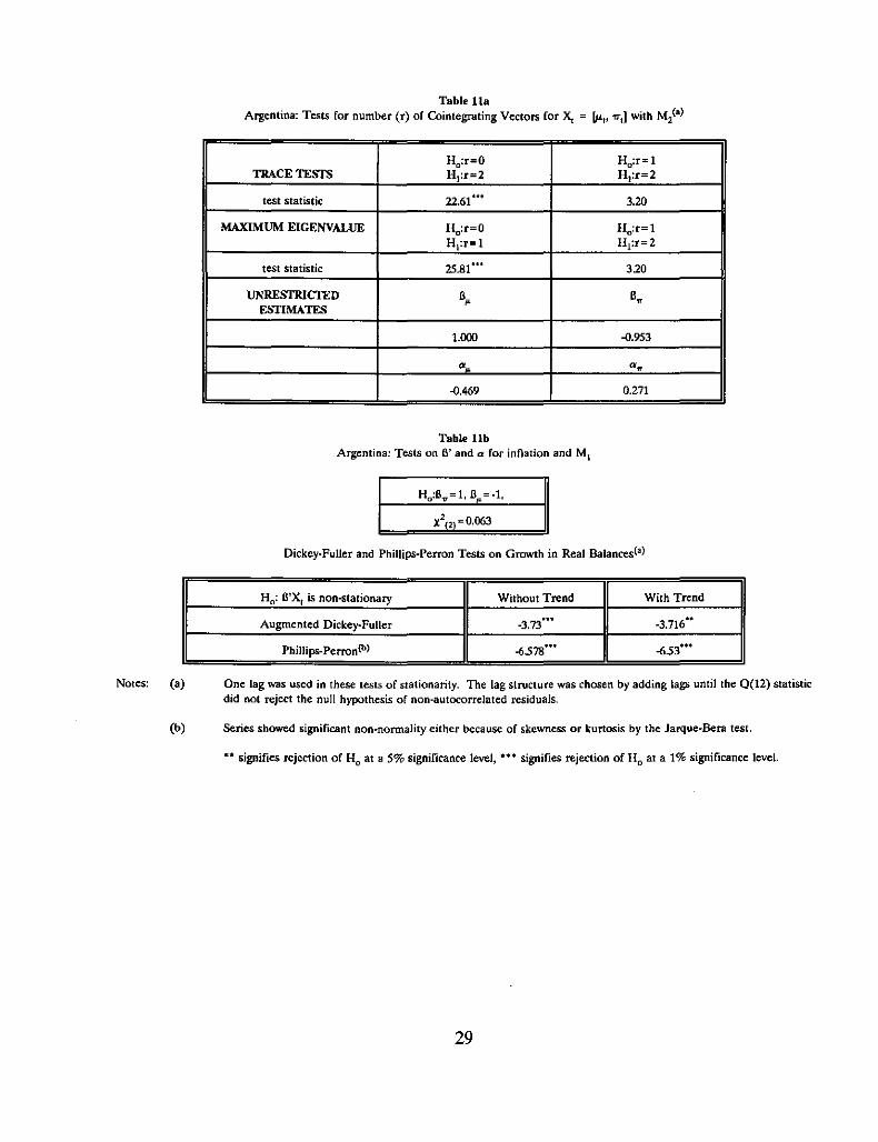
Table l1aArgentina: Tests for number (r) of Cointegrating Vectors for ~ = LuI' ?TIl with M2(a)

Ho:r=O Ho:r= 1TRACETEsrs H1:r=2 H1:r=2

test statistic 2261"· 3.20

MAXIMUM EIGENVALUE Ho:r=O Ho:r=1HI:r=1 H1:r=2

test statistic 25.81"· 320

UNRESfRlCTED B. B.ESTIMATES

1.000 -0.953

'" "'.-0.469 0.271

Table libArgentina: Tests on B' and a for inflation and M1

x'", =0.063

Dickey~Fuller and Phillips-Perron Tests on Growth in Real Balances(a)

Ho: SIX, is non-stationary Without Trend With Trend

Augmented Dickey.Fulier -3,73·" -3.716"

Phillips-Perron(b) -6578··· -653"·

Notes: (aj One lag was used in these tests of stationarity. The lag structure was chosen by adding lags until the 0(12) statisticdid not reject the null hypothesis of non-autocorrelated residuals.

(b) Series showed significant non·normality either because of skewness or kurtosis by the Jarque-Bera test.

.. signifies rejection of Ho at a 5% significance level, ... signifies rejection of Ho at a 1% significance level.

29

Table UaBolivia: Test for number (r) of Cointegrating Vectors for X. = [p.l' '1rt ] with M2(8)

Ho:r=O Ho:r=lTRACE TEsrs H1:r=2 H t :r=2

test statistic 31.39'" 2.85

MAXIMUM EIGENVALUE H,,:r=O Ho:r= 1H t :r=l H t :r=2

test statistic 2854'" 2.85

UNRESTRICTED O. O~

ESTIMATES

1.000 -0.881

'" "'~

-0.532 0.598

Table 12bBolivia: Tests on B' and Of for inflation and M2

X'(2) = 3.239'

Dickey·Puller and Phillips-Perron Tests on Growth in Real Balances(a)

Ho: S'x. is non-stationary Without Trend With Trend

Augmented Dickey-Fuller -7.84·" -3.716"

Phillips-Perron(b) -9.660'" -6.53"·

Notes: <aJ Two lags were used in these tests of stationarity. The lag structure was chosen by adding lags until the 0(12) statisticdid not reject the null hypothesis of non-autocorrelated residuals.

(b) Series showed significant non-nonnality either because of skewness or kurtosis by the Jarque-Bera test.

•• signifies rejection of Ho at a 5% significance level, ••• signifies rejection of Ho at a 1% significance level.

30

Table 13aBrazil: Tests for number (r) of Cointegrating Vectors for X. = I'"t, tJ-t] with Mz(a)

Ho:r=O Ho:r=1TRACE TESTS "l:r =2 "l:r =2

test statistic 27,66"· 0.42

MAXIMUM EIGENVALUE "o:r=O Ho:r= 1H1:r=1 H1:r=2

test statistic 28,07"· 0.42

UNRESfRlCTED B, B.ESTIMATES

1.000 .(l.907

a. a•

.(l.800 0.Q78

Table 13bBrazil: Tests on 13' and a for inDation and Mz

X'm=IA05

Dickey-Fuller and Phillips-Penon Tests on the Final B'X,(8)

Ho: 13'X. is non'1ltationary Without Trend With Trend

Augmented Dickey-Fuller -2.77· -2.78

Phillips-Perron -12.28'" -12.23'"

Notes: (aJ One lag was used in these tests of stationarity. The lag structure was chosen by adding lags until the 0(22) statisticdid not reject the null hypothesis of non-autocorrelated residuals.

.. signifies rejection of H o at a 10% significance level, U signifies rejection of H o at a S% significance level, ....signifies rejection of Ho at a 1% significance level.

31

Table 14aMexico: Tests for number (r) of Cointegrating Vectors for X. = [12",. Jitl with M, (a)

Ho:r=O Ho:r=1TRACE TESTS H1:r=2 "l: r =2

test statistic 54.75·" 5.91

MAXIMUM EIGENVALUE H,,:r=O "o:r= 1H t:r=1 . .J-It:r= 2

test statistic 48.84"· 5.91

UNRESTRICfED 6. 6~

ESTIMATES

1.000 -0.698

a. a~

-0.924 0.154

Table 14bMexico: Tests on 8' and Ct for inflation and M j

Dickey-Fuller and Phillips-Perron Tests on the Final 6'X.(a)

Ho: 6'X. is non·stationary Without Trend With Trend

Augmented Dickey-Fuller -4.'!"t•• -2.78

Phillips·Perron -18.04"· -12.23"·

Notes: (al Six lags were used in these tests of stationarity. The lag structure was chosen by adding lags until the 0(22) statisticdid not reject the null hypothesis of non·autocorrelated residuals.

,. signifies rejection of Ho at a 10% significance level, ,.,. signifies rejection of Ho at a 5% significance level, "',..signifies rejection of Ho at a 1% significance level.

32

Table 153Peru: Tests for number (r) of Cointegrating Vectors for ~ = [1ft• JoLt] with M2(8)

"o:r=O "o:r= 1TRACE TESTS ".:r=2 "1:r =2


MAXIMUM EIGENVALUE "o:r=O H o:r=1"l:r =1 '"1:r =2


RESTRICTED ESTIMATES B B~

1.000 -0.007

a. a~

-0.281 74.39

Table IShPeru: Tests on B' and a for inflation and M2

x'm =22.651'"

Dickey-Fuller and Phillips-Perron Tests on the Final B'X,(II)

"0: 8'~ is non-stationary Without Trend With Trend

Augmented Dickey-Fuller -1.922 -2.7B

Phillips-Perron ·3.91'" -12.23'"

Notes: (a) One lag was used in these tests of stationarity. The lag structure was chosen by adding lags until the Q(22) statisticdid not reject the null hypothesis of non-autocorrelated residuals.

• signifies rejection of Ho at a 10% significance level, .. signifies rejection of "0 at a 5% significance level, ...signifies rejection of "0 at a 1% significance level.

33

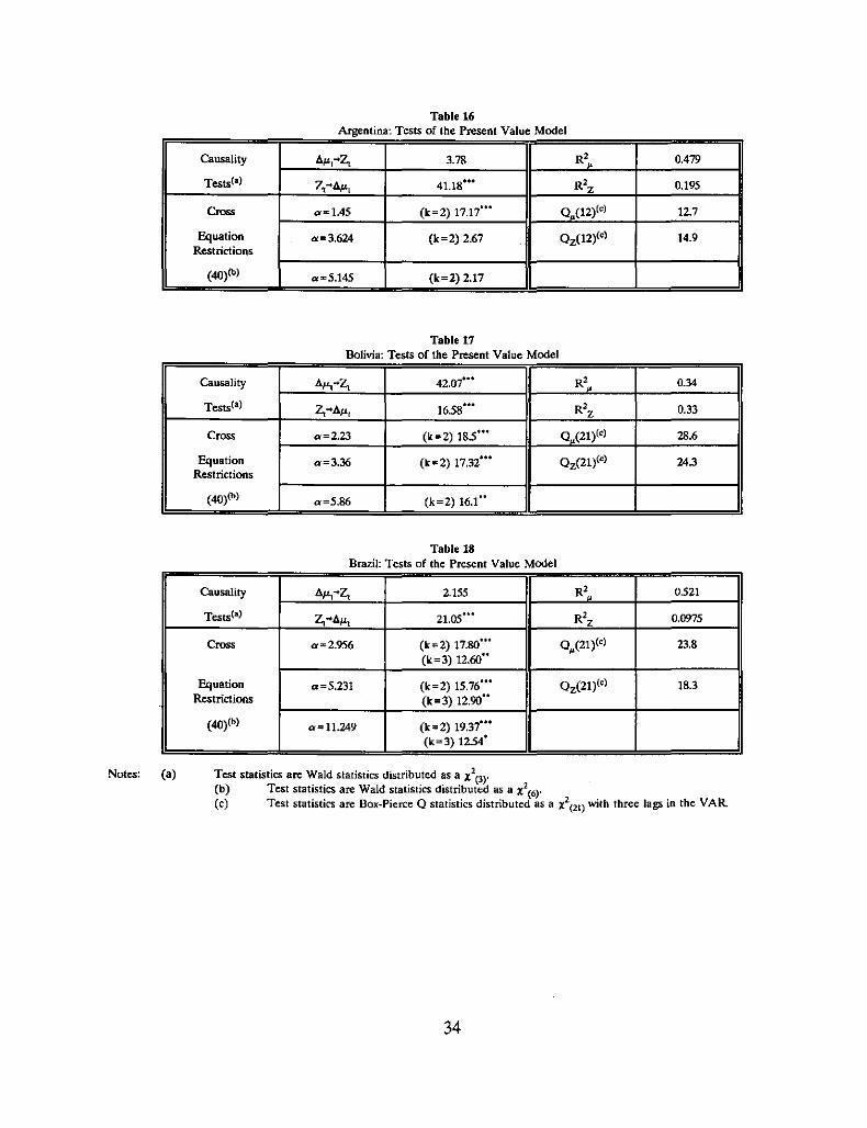
Table 16Argentina' Tests of the Present Value Model

Causality 11p.,~z, 3.78 R' 0.479

Tests(a)Z,~A", 41.18"· R' 0.195z

Cross a:o::1.45 (k=2) 17.17'" Q.(12)C') 12.7

Equation a. =3.624 (k=2) 2.67 Qz(l2)(') 14.9Restrictions

(4O)(b) a =5.145 (k=2) 2.17

Table 17Bolivia' Tests of the Present Value Model

Causality 11p.,~Z, 42.07"· R'. 0.34

Tests(a)Z,~A", 16.58'" R' 0.33z

Cross 0/=2.23 (k=2) 185'" Q.(21)C') 28.6

Equation a=3.36 (k=2) 17.31''' Qz(21)(') 24.3Restrictions

(4O)(b) «=5.86 (k=2) 16.1"

Table 18Brazil' Tests of the Present Value Model

Causality 11p.,~Z, 2.155 R'. 0521

Tests(a) z,".6.JLt 21.05'" R' 0.0975z

Cross a=2.956 (k=2) 17.80'" Q/2l)C') 23.8(k=3) 12.60"

Equation a=5.231 (k=2) 15.76'" Qz(21)C') 18.3Restrictions (k=3) 12.90"

(40)<") a= 11.249 (k=2) 19.37'''(k=3) 1254'

Notes: (a) Test statistics are Wald statistics distributed as a X2(3)'(b) Test statistics are Wald statistics distributed as a X2(6)'

(c) Test statistics are Box-Pierce 0 statistics distributed as a X2(21) with three lags in the VAR

34

Table 19Mexico' Tests of the Present Value Model

Causality Al't~Z. 15.5"" R'. 0.43

Tests(a)~"'AJ.Lt 23.67"" R' 0.01z

Croos a=2.27 (k=2) 9.29 o (21)(') 45.7

Equation «=3.24 (k=2) 9.07 Oz(21}i') 43.0Restrictions

(4O)(b) a=4.78 (k=2) 8.34

Table 20Peru' Tests of the Present Value Model

Causality AJ.Lt"'z,. 7.91u

R'. 0.43

Tests(a)Z.~lI.l't 25.17'" R' 0.01z

Croos 0=1.08 (k=2) 9.07 0.(21)(') 21.4

Equation «=3.66 (k=2) 7.07 Oz(21)(') 14.6Restrictions

(40)(b) a= 15.56 (k=2) 19.38'"

Notes: (a) Test statistics are Wald statistics distributed as a X2(3)'(b) Test statistics are Wald statistics distributed as a X2(6)'(e) Test statistics are Box·Pierce Q statistics distributed as a X2(21) with three Jags in the VAk

35

c:"!:C

J)

•--S;-co-Q

jG

l-..-:::ICC

l-

.->-

u...c- Co:!EiliC:;:;C8,..ce

~od'"

HB6~

£HB6~

£HB6~

£HB6~

£HB6~

£HL6~

£~-BL6~

£HL6~

£HL6i

£~-~m

£HL6~

£Hm

£HL6~

£l-~m

>!!~q0

9OS-q·.J

tilO~

<::.6>

9Q

).c<::

Sg-q·.J.2~

O~

:c<ll9

'iiiEgg-q•.J

~O~

<::Q

)

01'iii

90

WN0

1<ll

L9-q·.J0

1a.

....Ol

•....09

CD

01

....99-q·.J

eN

OO~

CD

;..

III9

::J;:

DIe

gg-q•.Ji!>

o.s::.O~

- e09

::Eiiitg-q·.J

:~Ol

'09

III<::.21;j

rg-q·.J=<::."

OtQ

)

§:;9

::c19-q·.J

O~

9~g-~•.J

O~9

#.#.

~~

#.#.

#.#.

00

~0

88

80

00

0ci

ci0

cici

cici

ciC

\I0

ex><D

....C

\I~

~~

Ol9l-g96lOl9l-j>96LOl9H

96

lOl9l-l9

6l

Ot9l-196lOl9l-096lOl9l-6

L6

l

Ol9l-8L

6l

019l-LL

6l

019l-9L

6t

Ol9l-gL61

O(

l'#.

~~

'#.'#.

'#.'#.

'#.'#.

00

80

00

00

00

00

00

C<0

C<,..;

<0.,;

.,fC'i

C\i~

0~,

.~m

C')C

GI.~

...-=III0);;::::-C

u.._>:c- co:::E

14.00%

12.00%

10.00%

8.00%

6.00%

4.00%

2.00%

0.00%

-2.00%

Figure 4Mexico: Monthly Inflation 1960:2-1989:9

Debt Crisisand Devaluation

Pacto Stabilization

~06-qaJ

II8~68-qaJ

Ll

8~88-qaJ

Il8~L8-qaJ

It8~98-qaJ

IIS~~s-qaJ

IIS~vs-qaJ

It8~£s-qaJ

IIS~

1-----1

1-----1

----+

---+

---+

----"-1

-ls-qaJ

CP.0Q

)Q

)...~('\IC

D.,

Q)

e:...

"g.L

l)c0

.c0

1·-

e:"

'Sj

:::J_

m-

.-c

LL

-:E

~11l

.c7ii

-)(

c~

0::!:O

l

:::JQ

j.<:

..~~

~11lC!l

"#8cico

"#8g

Figure 6Argentina: Monthly Real M2 Growth 1971:1-1984:2

30.00%

25.00%

20.00%

15.00%

10.00%

5.00%

0.00%1 I \ , , , , , 1 I 1 I

I

~~~\I\I~-5.00% , V~ V§ \/§ V V~

-10.00%

-15.00%

-20.00%

~

I

""=0>

g-qa.:l

Ol9gg-qa.:l

Ol

Q)

90

Lg-qa.:lQ

)Q

)....

Ol•N0

9coQ

)....

....s:.

l!!~~...2""U

-N::i0

iiiCIlII:III

:~'0m

'#~

'#'#

'#0

00

00

00

00

00

00

0C

\IC)l

'Yco,

4.00%

3.00% ~

2.00%

1.00%

-2.00%

-3.00% L

Figure 8Brazil: Monthly Real M2 Growth 1974:2-1985:12

A ~h,' ,11.1,

"b'~ I " ,,"!:' «> o "". «: ~ic; b ;:' «> ~ N <::> N p ~ F;< o~= <::>

I "<::>-~ I - I

f\~ ~ ~

IA

15.00%

10.00%

5.00%

0.00%

-5.00%

-10.00%

Figure 9Mexico: Real Monthly M1 Growth 1960:2 to 1989:9

69-

CD

00)

0)

....•NNco0)

-qa.:l......t::

t~

O~

9.......C

1)t'9

"'N

5J:=99-q

a.:lu:::~

Ll..t::

- c:::9

0:=IIIII::::J...C

I)D

.

qa.:l

Appendix: Tests of Stability

This appendix shows the results of CUSUM calculations for the inflation model in

Argentina, Bolivia, Brazil, Mexico, and Peru.' The CUSUMs are calculated based upon

the recursive residuals from the first equation of the VARin equation (28) in the text of

the following form

(AI)

The CUSUM series are presented in Figures Al through AS along with 5% and

10% confidence bands. None of the series cross the significance bounds indicating no

significant structural change. Sharp movements in the series, however, might indicate

structural break. Argentina, (1980-81, 1983), Bolivia (1985), Mexico (1982-83, and Peru

(1988 and 1990) show some moderate movements in the CUSUM series. Still,

permanent regime changes and structural instability do not seem to be indicated by the

data.

'For a good discussion of recursive residuals and CUSUM, see Harvey (1990).

\~

II

H961

\,

tI

f\

If

\I

I\

-£96~

If

II

f\

,J

f\

,J

I\

"I

I\:

II

\:f

I\:

fI

\:6~

If

\"

fI

\"

II

c:'!\

"f

f"'"

\"

fI

ao01

\"

ff

...,\:

II

...~\:

~I

I...

01

\"

If

ce'"\

"l-6l6~

II

CIl:E

t"::::l

\:I

I6,(1)

\"

II

.-::::l

11

.0\:

/Iiii

I'./I

c\

"/I

:;:::c\

"1/

CIlC

l\

"JI

..ce\

"fI

\"

£1/

\"

~II

\"

Hl6~

II\

"t

1/\

"£

1/\:

~II

\:~-~m

II\

"t

III:

£II

\:~

/I\

"H

l6l

/I\

"t

/I\

"£

II\:

~1/

'"0

'"0

'"0

'90

'"0

'"C

\IC

\I~

~~

~C)J

C)J,

,

B,

~•,

l,,

~l,,,

B,.,

~,,

l,•

~~

··,B

,,~

,•l

.,II

,B

,·co

·~

0· ,

Ol

,l

,O

l,

-,

li,

06

--N';':9

«co9B-JON

al

Ol

·..-

··li

:::l::E,

.21~

,,6

LL

CI)

,•~

,9

0,,

~B-JON

co,,

:?i,

II,.

'06

IIIvB-unr

,vB-JON

.,li

,

6

•~B-unr

,,~B-JON

,,II

,,•6

•,9

,,lB-JO

N,.

II,,

6,,,

~B-U

,

~0

00

00

0~

~~

"?~

,

,,

96,,

L,:

£,,-96,

,,L

,

£,

,,-,"

L:::

,-Z961,,,

C\ol,..

,,H

96

,an

,coa!

,..•£

,..,..,

M..

,1-096,ce;;!:

,,a

la!

L...

,..s,::::E

::£

.-::J

LLVJ

,"-6

m::J

,0

,L

'i:

£:

...,

"-9

mlD

,,,L

:£,H

m,,

L

,£

,,IH

L6

,,

L

,£,H

L6

,,L

,,££

00

00

00

0C

\l~

";"C)l

'?"'I'

\::t:

L\i

69\\

-UO

r1

L\\

99-uor

IL

\\L9

\-uor

\L

\99

\-uor

\IL

\,9

I-uor

\\L

\t9

\-uor

C?!\

L\

£9al

1Q

)1

-UO

ral

\.-

\L

\0

i19

-\

-UO

r':':

1L

0::1'.-\

CC"'"\

19a

lal

-uor..

'-

\::::l:E

IL

~~

\09

\Il.U

J\

-uor~

\

0\

L\

6L0

\\-uor

u\

";C\

Lal

\9L

:E\1

-uor\\

L\

LLi

-uor\

LI

9L\\

-uori

LI\

gL\\

-uor\

L1\

tL\\

-uor\

L\

£L

\-uor

\L

\lL

\-uor

5lS?

~0

00

00

00

0C

\I~

";"C)I

<?.,

~

6- uor

69- uorOlLV99- uor

01co0

L0

)0

)...

VI

...1I)eW

)9- uor

-tClCl

cpO

).....~:i!

.~::::lU

-(j)::::l

V(,)

:i..cpa..

v~9-uor

01LVv9- uor

O~LV

00

00

00

C\l

~~

Cl'"?

,

Documents

Research Paper - Dallasfed.org/media/documents/research/papers/1992/... · Research Paper Federal Reserve Bank ... of the initial orthodox adjustment and acceleration of inflation,