research papers

IUCrJ (2018). 5, 531–541 https://doi.org/10.1107/S2052252518010047 531

IUCrJISSN 2052-2525

PHYSICSjFELS

Received 8 March 2018

Accepted 11 July 2018

Edited by E. E. Lattman, University at Buffalo,

USA

Keywords: XFELs; Melbournevirus; coherent

diffractive imaging; LCLS; image reconstruction.

Supporting information: this article has

supporting information at www.iucrj.org

Considerations for three-dimensional imagereconstruction from experimental data incoherent diffractive imaging

Ida V. Lundholm,a Jonas A. Sellberg,b Tomas Ekeberg,a Max F. Hantke,c Kenta

Okamoto,a Gijs van der Schot,a Jakob Andreasson,a,d,e Anton Barty,f Johan

Bielecki,a,g Petr Bruza,e Max Bucher,h,i,j Sebastian Carron,h Benedikt J. Daurer,a

Ken Ferguson,h,k Dirk Hasse,a Jacek Krzywinski,h Daniel S. D. Larsson,a Andrew

Morgan,f Kerstin Muhlig,a Maria Muller,i Carl Nettelblad,a,l Alberto Pietrini,a

Hemanth K. N. Reddy,a Daniela Rupp,i Mario Sauppe,i Marvin Seibert,a Martin

Svenda,a Michelle Swiggers,h Nicusor Timneanu,a,m Anatoli Ulmer,i Daniel

Westphal,a Garth Williams,h,n Alessandro Zani,a Gyula Faigel,o Henry N.

Chapman,f Thomas Moller,i Christoph Bostedt,h,j,k,p Janos Hajdu,a,d Tais

Gorkhoverh,i,k and Filipe R. N. C. Maiaa,q*

aLaboratory of Molecular Biophysics, Department of Cell and Molecular Biology, Uppsala University, Husargatan 3 (Box

596), SE-751 24 Uppsala, Sweden, bBiomedical and X-ray Physics, Department of Applied Physics, AlbaNova University

Center, KTH Royal Institute of Technology, SE-106 91 Stockholm, Sweden, cUniversity of Oxford, UK, dELI Beamlines,

Institute of Physics, Czech Academy of Science, Na Slovance 2, CZ-182 21 Prague, Czech Republic, eCondensed Matter

Physics, Department of Physics, Chalmers University of Technology, Gothenburg, Sweden, fCenter for Free-Electron Laser

Science, DESY, Notkestrasse 85, 22607 Hamburg, Germany, gEuropean XFEL GmbH, Holzkoppel 4, 22869 Schenefeld,

Germany, hLinac Coherent Light Source, SLAC National Accelerator Laboratory, Stanford, California 94309, USA, iInstitut

fur Optik und Atomare Physik, Technische Universitat Berlin, Hardenbergstr. 36, 10623 Berlin, Germany, jChemical

Sciences and Engineering Division, Argonne National Laboratory, 9700 South Cass Avenue, Lemont, IL 60439, USA,kPULSE Institute and SLAC National Accelerator Laboratory, 2575 Sand Hill Road, Menlo Park, CA 94025, USA, lDivision

of Scientific Computing, Department of Information Technology, Science for Life Laboratory, Uppsala University,

Lagerhyddsvagen 2 (Box 337), SE-751 05 Uppsala, Sweden, mDepartment of Physics and Astronomy, Uppsala University,

Box 516, SE-751 20 Uppsala, Sweden, nNSLS-II, Brookhaven National Laboratory, PO Box 5000, Upton, NY 11973,

USA, oResearch Institute for Solid State Physics and Optics, 1525 Budapest, Hungary, pDepartment of Physics,

Northwestern University, 2145 Sheridan Road, Evanston, IL 60208, USA, and qNERSC, Lawrence Berkeley National

Laboratory, 1 Cyclotron Rd, Berkeley, CA 94720, USA. *Correspondence e-mail: filipe@xray.bmc.uu.se

Diffraction before destruction using X-ray free-electron lasers (XFELs) has the

potential to determine radiation-damage-free structures without the need for

crystallization. This article presents the three-dimensional reconstruction of the

Melbournevirus from single-particle X-ray diffraction patterns collected at the

LINAC Coherent Light Source (LCLS) as well as reconstructions from

simulated data exploring the consequences of different kinds of experimental

sources of noise. The reconstruction from experimental data suffers from a

strong artifact in the center of the particle. This could be reproduced with

simulated data by adding experimental background to the diffraction patterns.

In those simulations, the relative density of the artifact increases linearly with

background strength. This suggests that the artifact originates from the Fourier

transform of the relatively flat background, concentrating all power in a central

feature of limited extent. We support these findings by significantly reducing the

artifact through background removal before the phase-retrieval step. Large

amounts of blurring in the diffraction patterns were also found to introduce

diffuse artifacts, which could easily be mistaken as biologically relevant features.

Other sources of noise such as sample heterogeneity and variation of pulse

energy did not significantly degrade the quality of the reconstructions. Larger

data volumes, made possible by the recent inauguration of high repetition-rate

XFELs, allow for increased signal-to-background ratio and provide a way to

minimize these artifacts. The anticipated development of three-dimensional

Fourier-volume-assembly algorithms which are background aware is an

alternative and complementary solution, which maximizes the use of data.

1. Introduction

X-ray crystallography has for decades been the major tech-

nique to solve the structure of proteins, but one of the

bottlenecks is the production of well-diffracting crystals. The

method of flash X-ray imaging (FXI) aims to record diffrac-

tion directly from single macromolecules (Neutze et al., 2000)

and has the potential to allow structure determination of

biological particles without the time-consuming crystallization

step. By studying single particles it is possible in principle to

capture conformational substates that would otherwise not be

detectable from the averaged ensemble of a crystal. Once the

technique matures, there is a tremendous potential in FXI to

study conformational heterogeneity as well as time-resolved

structural changes of biological samples (Spence, 2017).

Instead of getting the diffraction signal enhanced by repeating

units of the protein in a crystal into strong Bragg peaks, FXI

leans on a sufficiently bright X-ray pulse. Unfortunately, the

high-intensity X-ray radiation needed to measure a single

particle’s diffraction pattern completely obliterates the sample

because of radiation damage. Theoretical work has shown that

femtosecond pulses of intense X-ray radiation produced by

free-electron lasers can outrun the key radiation-damage

processes (Neutze et al., 2000; Jurek et al., 2004; Bergh et al.,

2008) and produce a diffraction pattern of a practically

damage-free particle. This ‘diffraction before destruction’

method was successfully employed experimentally for the first

time in 2006 (Chapman, Barty, Bogan et al., 2006). Since then

the technique has been used to determine low-resolution two-

dimensional images from single diffraction patterns of several

biological samples including cells (Mancuso et al., 2010;

Seibert et al., 2010; Schot et al., 2015), cell organelles (Hantke

et al., 2014) and virus particles in two dimensions (Seibert et al.,

2011; Kassemeyer et al., 2012; Daurer et al., 2017) and three

dimensions (Ekeberg et al., 2015; Kurta et al., 2017).

In FXI, only the modulus squared of the Fourier transform

of the particle can be measured and the phase of the diffracted

wavefunction has to be determined in order to reconstruct the

object. The diffraction pattern of a single particle is contin-

uous, which makes it possible to determine the phase

computationally through an iterative process (Fienup, 1978).

Two constraints are enforced in iterative phase retrieval. The

first constrains the Fourier amplitudes to be consistent with

the experimental intensities and the second constrains the

object to reside within a limited real-space volume, also known

as the support (Marchesini et al., 2003).

For three-dimensional imaging there is the additional

problem of the unknown orientations of the particles, which

have to be retrieved in order to build up a three-dimensional

diffraction volume from which a three-dimensional image can

be reconstructed (Loh et al., 2010). Since the particles arrive in

the X-ray focus with a random orientation, the rotations have

to be determined computationally from the noisy diffraction

patterns. Imaging in three dimensions requires sample

homogeneity, either within the full data set or a homogeneous

subset of the data (Maia et al., 2009), and thus requires careful

image selection in order to obtain a good reconstruction. The

rotation problem as well as the requirement for homogeneity

of the image set makes three-dimensional imaging with FXI

more challenging than the single-shot two-dimensional

imaging case, which can be performed on non-reproducible

objects.

In the experiment, single particles are typically introduced

into the X-ray beam as a stream of free particles in a vacuum,

thereby circumventing the need for a substrate that would

yield unnecessary background scattering. Even so, back-

ground scattering from optical components of the beamline as

well as from gas used during sample delivery is still present in

the data. Assuming the sample is homogeneous, the strength

of the signal can be increased, compared with the background,

by averaging diffraction patterns with identical orientations

(Huldt et al., 2003).

In this article, we present a three-dimensional reconstruc-

tion of a 230 nm icosahedral virus, the Melbournevirus (MelV)

at 28 nm resolution from experimental FXI data. The recon-

struction contains a central region with twice the density of the

surrounding particle. This difference is larger than what would

be expected from any biological sample, pointing to it being a

reconstruction artifact. To understand what may cause this

artifact, we study the effects that background, sample

heterogeneity and diffraction-space blurring have on the

quality of FXI three-dimensional reconstructions using simu-

lated data.

2. Methods

2.1. Data collection

The experiment was performed with the LAMP instrument

(Ferguson et al., 2015) at the AMO endstation (Bozek, 2009)

of the LINAC Coherent Light Source (LCLS) free-electron

laser (Emma et al., 2010). The sample was aerosolized with a

gas-dynamic virtual nozzle (GDVN) and delivered into the

X-ray focus as a stream of isolated particles using a purpose-

built aerosol particle injector (Seibert et al., 2011; Hantke et al.,

2014). Far-field diffraction of the aerosolized particles was

detected by a pnCCD detector (Struder et al., 2010) positioned

0.732 m downstream of the interaction region and monitored

using Hummingbird (Daurer et al., 2016). The detector

consisted of two detector halves separated by 1.19 mm with a

total size of 1024� 1024 pixels and a pixel size of 75 � 75 mm.

Data were recorded during an X-ray Fourier holography

experiment (Gorkhover et al., 2018), where Xe clusters with an

average diameter of 30–120 nm were used as holographic

reference and were produced at 10–30 Hz via a supersonic

expansion from a separate cluster injector. The free-electron

laser was operated at 1.2 keV photon energy (corresponding

to an X-ray wavelength of about 1.0 nm) producing �100 fs

long pulses of �2 mJ at 120 Hz repetition rate. The X-ray

beam was focused by a pair of Kirkpatrick–Baez mirrors down

to nominally �2 � 2 mm in order to achieve intensities at the

interaction region necessary for FXI. The actual intensity on

the sample was estimated to 0.01 mJ mm�2 by performing a

research papers

532 Ida V. Lundholm et al. � Image reconstruction in coherent diffractive imaging IUCrJ (2018). 5, 531–541

low-resolution spherical fit according to x2.4 and described in

detail in Daurer et al. (2017).

2.2. Data preprocessing

Preprocessing of the raw data was performed with the

Cheetah software package (Barty et al., 2014). The relative

positions of the detector halves with respect to the X-ray beam

axis were recovered from diffraction data of Xe clusters with

intense and sharp Newton rings covering both halves, which

yielded a horizontal separation of 1.19 mm and a vertical

displacement of 0.24 mm. Electronic noise was accounted for

by (i) subtracting a dark-frame average of �4000 frames

recorded prior to the X-ray exposure, and (ii) performing a

common-mode correction where the zero-photon peak was

determined individually for each line in the detector halves

and subtracted on a shot-by-shot basis. Polarization correction

and solid-angle correction were performed as described in

Sellberg et al. (2014). Additionally, a photon background

(created from the median intensity of the last 100 non-hit

frames using Cheetah’s running background algorithm),

consisting of stray X-rays not properly focused, was

subtracted. Finally, defective pixels with non-linear detector

responses were masked out, as determined by a pixel-by-pixel

gain map with a nominal gain of 95 analog-to-digital units

(ADU) per photon. In particular, saturated pixels (above

10 000 ADU), hot pixels (90% of the last 100 frames above

5000 ADU) and noisy pixels (whose standard deviations of the

last 100 background frames are above 500 ADU) were also

considered defective.

2.3. Selection of diffraction patterns

Hit selection occurred in multiple steps. In the first stage we

used a threshold on the number of lit pixels to find hits. Pixels

with a value above 250 ADU, corresponding roughly to 3-

photon events or more, were considered lit. The minimum

number of lit pixels required to consider an image a hit was set

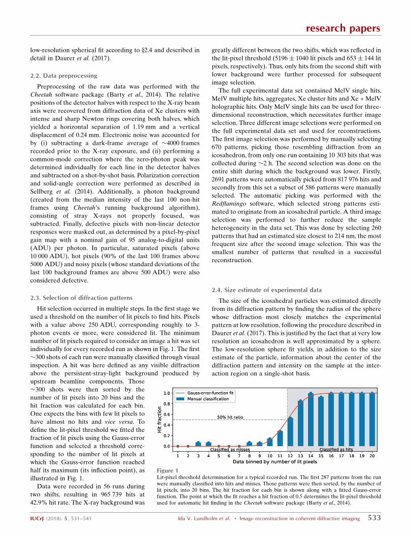
individually for every recorded run as shown in Fig. 1. The first

�300 shots of each run were manually classified through visual

inspection. A hit was here defined as any visible diffraction

above the persistent-stray-light background produced by

upstream beamline components. Those

�300 shots were then sorted by the

number of lit pixels into 20 bins and the

hit fraction was calculated for each bin.

One expects the bins with few lit pixels to

have almost no hits and vice versa. To

define the lit-pixel threshold we fitted the

fraction of lit pixels using the Gauss-error

function and selected a threshold corre-

sponding to the number of lit pixels at

which the Gauss-error function reached

half its maximum (its inflection point), as

illustrated in Fig. 1.

Data were recorded in 56 runs during

two shifts, resulting in 965 739 hits at

42.9% hit rate. The X-ray background was

greatly different between the two shifts, which was reflected in

the lit-pixel threshold (5196 � 1040 lit pixels and 653� 144 lit

pixels, respectively). Thus, only hits from the second shift with

lower background were further processed for subsequent

image selection.

The full experimental data set contained MelV single hits,

MelV multiple hits, aggregates, Xe cluster hits and Xe + MelV

holographic hits. Only MelV single hits can be used for three-

dimensional reconstruction, which necessitates further image

selection. Three different image selections were performed on

the full experimental data set and used for reconstructions.

The first image selection was performed by manually selecting

670 patterns, picking those resembling diffraction from an

icosahedron, from only one run containing 10 303 hits that was

collected during �2 h. The second selection was done on the

entire shift during which the background was lower. Firstly,

2691 patterns were automatically picked from 817 976 hits and

secondly from this set a subset of 586 patterns were manually

selected. The automatic picking was performed with the

Redflamingo software, which selected strong patterns esti-

mated to originate from an icosahedral particle. A third image

selection was performed to further reduce the sample

heterogeneity in the data set. This was done by selecting 260

patterns that had an estimated size closest to 214 nm, the most

frequent size after the second image selection. This was the

smallest number of patterns that resulted in a successful

reconstruction.

2.4. Size estimate of experimental data

The size of the icosahedral particles was estimated directly

from its diffraction pattern by finding the radius of the sphere

whose diffraction most closely matches the experimental

pattern at low resolution, following the procedure described in

Daurer et al. (2017). This is justified by the fact that at very low

resolution an icosahedron is well approximated by a sphere.

The low-resolution sphere fit yields, in addition to the size

estimate of the particle, information about the center of the

diffraction pattern and intensity on the sample at the inter-

action region on a single-shot basis.

research papers

IUCrJ (2018). 5, 531–541 Ida V. Lundholm et al. � Image reconstruction in coherent diffractive imaging 533

Figure 1Lit-pixel threshold determination for a typical recorded run. The first 287 patterns from the runwere manually classified into hits and misses. Those patterns were then sorted, by the number oflit pixels, into 20 bins. The hit fraction for each bin is shown along with a fitted Gauss-errorfunction. The point at which the fit reaches a hit fraction of 0.5 determines the lit-pixel thresholdused for automatic hit finding in the Cheetah software package (Barty et al., 2014).

2.5. Simulation of diffraction data

Two-dimensional and three-dimensional diffraction images

were simulated using the Condor software (Hantke et al.,

2016). An electron cryomicroscopy (cryo-EM) structure of

MelV (Okamoto et al., 2018) was used as input for the simu-

lations. The inside of the virus particle, not resolved in the

cryo-EM model, was set to a uniform density. The relative

electron density between capsid, membrane and interior of the

particle was estimated from a tomographic reconstruction of

MelV from cryo-EM data. 1000 diffraction images were

simulated with random particle orientations and then Poisson

sampled prior to their reconstruction. X-ray wavelength, pulse

energy and detector distance were chosen to match the

experiment.

2.6. Three-dimensional reconstruction pipeline

Three-dimensional reconstructions for experimental data

and simulated data were performed using the same pipeline.

Two-dimensional images were oriented with the EMC algo-

rithm (Expand, Maximize and Compress) (Loh & Elser, 2009;

Loh et al., 2010) using the same implementation as in Ekeberg

et al. (2015). Both simulated and experimental data were

downsampled eight times in all directions from 1024� 1024

pixels to 128� 128 pixels prior to image orientation. Experi-

mental data were also centered according to the diffraction-

pattern center that was retrieved from the sphere fit

mentioned above.

Phase retrieval in three dimensions was performed with the

Hawk software package (Maia et al., 2010). The phasing

protocol started with 6000 iterations of the RAAR algorithm

(Luke, 2005) enhanced with a positivity constraint (Marche-

sini et al., 2003). The first 1000 iterations of RAAR were run

with a large static spherical support with a 20-pixel radius

followed by 5000 iterations with a tight static spherical support

with a 12-pixel radius, corresponding to a diameter of 236 nm.

The reconstruction was then refined with 1000 iterations of

error reduction (Fienup, 1978). 1000 individual reconstruc-

tions were calculated and the final model is the average of

these. The reproducibility of the phase retrieval was checked

using the phase-retrieval transfer function (PRTF) (Chapman,

Barty, Marchesini et al., 2006). The resolution of the recon-

struction is estimated by the point at which the PRTF falls

below 1=e (Chapman, Barty, Bogan et al., 2006; Seibert et al.,

2011).

2.7. Real-space residual

The real-space residual (RSR) is a real-space validation tool

used in X-ray protein crystallography to assess the resem-

blance between the electron density calculated from experi-

mental structure factors and calculated structure factors from

the model on a residue basis (Jones et al., 1991). Here, the real-

space residual is calculated on a voxel basis and compares the

difference in electron density between the average recon-

structed model (�rec) and a support object with a uniform

density of one (�sup). The RSR was calculated for voxels

where the density of the average reconstructed model is above

10% of the maximum density according to

RSR ¼

Pj�rec � �supjPj�rec þ �supj

: ð1Þ

3. Results and discussion

3.1. MelV reconstruction from experimental data

A three-dimensional reconstruction from single-particle

diffraction data requires sample homogeneity. Only a small

fraction of the one million hits collected in this experiment are

high-quality diffraction patterns of MelV. The first step was

therefore to select those high-quality diffraction patterns. In

this work, a high-quality diffraction pattern has a strong

scattered signal and clear icosahedral features. The selected

image set must also have a small size distribution, a require-

ment for sufficient sample homogeneity to allow for a

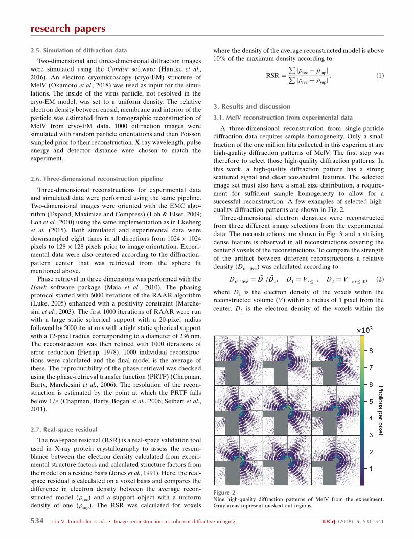
successful reconstruction. A few examples of selected high-

quality diffraction patterns are shown in Fig. 2.

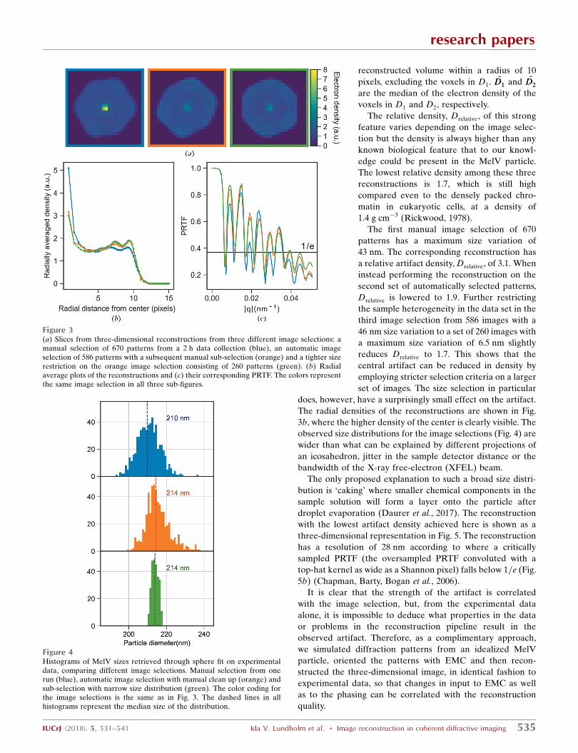
Three-dimensional electron densities were reconstructed

from three different image selections from the experimental

data. The reconstructions are shown in Fig. 3 and a striking

dense feature is observed in all reconstructions covering the

center 8 voxels of the reconstructions. To compare the strength

of the artifact between different reconstructions a relative

density (Drelative) was calculated according to

Drelative ¼~D1D1= ~D2D2; D1 ¼ Vr� 1; D2 ¼ V1< r� 10; ð2Þ

where D1 is the electron density of the voxels within the

reconstructed volume (V) within a radius of 1 pixel from the

center. D2 is the electron density of the voxels within the

research papers

534 Ida V. Lundholm et al. � Image reconstruction in coherent diffractive imaging IUCrJ (2018). 5, 531–541

Figure 2Nine high-quality diffraction patterns of MelV from the experiment.Gray areas represent masked-out regions.

reconstructed volume within a radius of 10

pixels, excluding the voxels in D1. ~D1D1 and ~D2D2

are the median of the electron density of the

voxels in D1 and D2, respectively.

The relative density, Drelative, of this strong

feature varies depending on the image selec-

tion but the density is always higher than any

known biological feature that to our knowl-

edge could be present in the MelV particle.

The lowest relative density among these three

reconstructions is 1.7, which is still high

compared even to the densely packed chro-

matin in eukaryotic cells, at a density of

1.4 g cm�3 (Rickwood, 1978).

The first manual image selection of 670

patterns has a maximum size variation of

43 nm. The corresponding reconstruction has

a relative artifact density, Drelative, of 3.1. When

instead performing the reconstruction on the

second set of automatically selected patterns,

Drelative is lowered to 1.9. Further restricting

the sample heterogeneity in the data set in the

third image selection from 586 images with a

46 nm size variation to a set of 260 images with

a maximum size variation of 6.5 nm slightly

reduces Drelative to 1.7. This shows that the

central artifact can be reduced in density by

employing stricter selection criteria on a larger

set of images. The size selection in particular

does, however, have a surprisingly small effect on the artifact.

The radial densities of the reconstructions are shown in Fig.

3b, where the higher density of the center is clearly visible. The

observed size distributions for the image selections (Fig. 4) are

wider than what can be explained by different projections of

an icosahedron, jitter in the sample detector distance or the

bandwidth of the X-ray free-electron (XFEL) beam.

The only proposed explanation to such a broad size distri-

bution is ‘caking’ where smaller chemical components in the

sample solution will form a layer onto the particle after

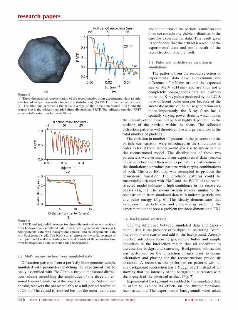
droplet evaporation (Daurer et al., 2017). The reconstruction

with the lowest artifact density achieved here is shown as a

three-dimensional representation in Fig. 5. The reconstruction

has a resolution of 28 nm according to where a critically

sampled PRTF (the oversampled PRTF convoluted with a

top-hat kernel as wide as a Shannon pixel) falls below 1=e (Fig.

5b) (Chapman, Barty, Bogan et al., 2006).

It is clear that the strength of the artifact is correlated

with the image selection, but, from the experimental data

alone, it is impossible to deduce what properties in the data

or problems in the reconstruction pipeline result in the

observed artifact. Therefore, as a complimentary approach,

we simulated diffraction patterns from an idealized MelV

particle, oriented the patterns with EMC and then recon-

structed the three-dimensional image, in identical fashion to

experimental data, so that changes in input to EMC as well

as to the phasing can be correlated with the reconstruction

quality.

research papers

IUCrJ (2018). 5, 531–541 Ida V. Lundholm et al. � Image reconstruction in coherent diffractive imaging 535

Figure 3(a) Slices from three-dimensional reconstructions from three different image selections: amanual selection of 670 patterns from a 2 h data collection (blue), an automatic imageselection of 586 patterns with a subsequent manual sub-selection (orange) and a tighter sizerestriction on the orange image selection consisting of 260 patterns (green). (b) Radialaverage plots of the reconstructions and (c) their corresponding PRTF. The colors representthe same image selection in all three sub-figures.

Figure 4Histograms of MelV sizes retrieved through sphere fit on experimentaldata, comparing different image selections. Manual selection from onerun (blue), automatic image selection with manual clean up (orange) andsub-selection with narrow size distribution (green). The color coding forthe image selections is the same as in Fig. 3. The dashed lines in allhistograms represent the median size of the distribution.

3.2. MelV reconstruction from simulated data

Diffraction patterns from a perfectly homogeneous sample

simulated with parameters matching the experiment can be

easily assembled with EMC into a three-dimensional diffrac-

tion volume resembling the amplitudes of the three-dimen-

sional Fourier transform of the object as intended. Subsequent

phasing recovers the phases reliably to a full-period resolution

of 20 nm. The capsid is resolved but not the inner membrane

and the interior of the particle is uniform and

does not contain any visible artifacts as in the

case for experimental data. This result gives

us confidence that the artifact is a result of the

experimental data and not a result of the

reconstruction pipeline itself.

3.3. Pulse and particle-size variation insimulations

The patterns from the second selection of

experimental data have a maximum size

difference of �20 nm around the expected

size of MelV (214 nm) and are thus not a

completely homogeneous data set. Further-

more, the X-ray pulses produced by the LCLS

have different pulse energies because of the

stochastic nature of the pulse generation and,

more importantly, the X-ray focus has a

spatially varying power density, which makes

the intensity of the measured pattern highly dependent on the

position of the particle within the focus. The collected

diffraction patterns will therefore have a large variation in the

total number of photons.

The variation in number of photons in the patterns and the

particle-size variation were introduced in the simulations in

order to test if these factors would give rise to any artifact in

the reconstructed model. The distributions of these two

parameters were estimated from experimental data (second

image selection) and then used as probability distributions in

the simulations to produce patterns with varying combinations

of both. The cryo-EM map was resampled to produce the

desired-size variation. The produced patterns could be

successfully oriented with EMC and the PRTF of the recon-

structed model indicates a high confidence in the recovered

phases (Fig. 6). The reconstruction is very similar to the

reconstruction from simulated data with uniform particle size

and pulse energy (Fig. 6). This clearly demonstrates that

variations in particle size and pulse-energy matching the

experiment do not pose a problem for three-dimensional FXI.

3.4. Background scattering

One big difference between simulated data and experi-

mental data is the presence of background scattering. Beam-

line components scatter and add to the background. Aerosol

injection introduces focusing gas, sample buffer and sample

impurities in the interaction region that all contribute to

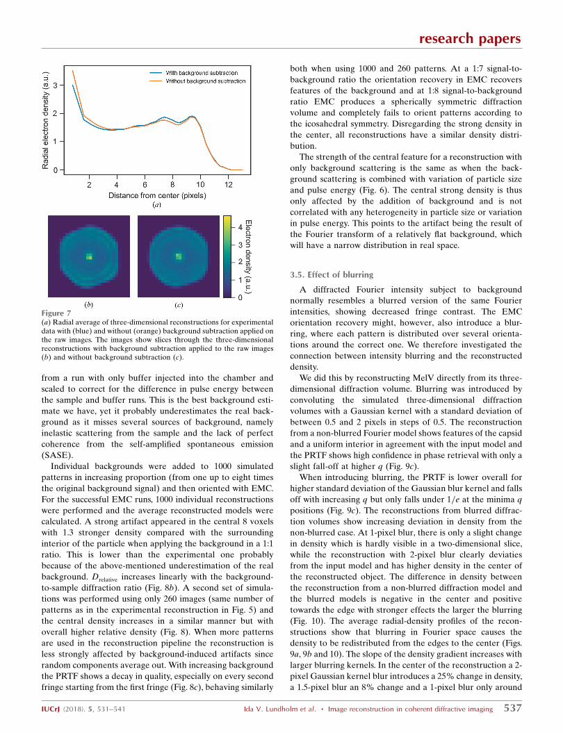
increase the background scattering. Background subtraction

was performed on the diffraction images prior to image

orientation and phasing for the reconstructions previously

discussed. A reconstruction performed on patterns without

any background subtraction has a Drelative of 2.1 instead of 1.7

showing that the intensity of the background correlates with

the strength of the observed artifact (Fig. 7).

Experimental background was added to the simulated data

in order to explore its effects on the three-dimensional

reconstructions. The experimental backgrounds were taken

research papers

536 Ida V. Lundholm et al. � Image reconstruction in coherent diffractive imaging IUCrJ (2018). 5, 531–541

Figure 5(a) Three-dimensional representation of the reconstruction from experimental data (a strictselection of 260 patterns with a limited size distribution). (b) PRTF for the reconstruction in(a). The blue line represents the radial average of the three-dimensional PRTF and theorange line is the critically sampled three-dimensional PRTF. The critically sampled PRTFshows a full-period resolution of 28 nm.

Figure 6(a) PRTF and (b) radial average for three-dimensional reconstructionsfrom homogeneous simulated data (blue), heterogeneous data (orange),homogeneous data with background (green) and heterogeneous datawith background (red). The black curve represents the radial average ofthe input model scaled according to central density of the reconstructionfrom homogeneous data without added background.

from a run with only buffer injected into the chamber and

scaled to correct for the difference in pulse energy between

the sample and buffer runs. This is the best background esti-

mate we have, yet it probably underestimates the real back-

ground as it misses several sources of background, namely

inelastic scattering from the sample and the lack of perfect

coherence from the self-amplified spontaneous emission

(SASE).

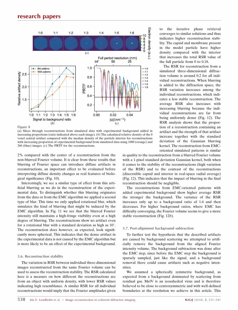
Individual backgrounds were added to 1000 simulated

patterns in increasing proportion (from one up to eight times

the original background signal) and then oriented with EMC.

For the successful EMC runs, 1000 individual reconstructions

were performed and the average reconstructed models were

calculated. A strong artifact appeared in the central 8 voxels

with 1.3 stronger density compared with the surrounding

interior of the particle when applying the background in a 1:1

ratio. This is lower than the experimental one probably

because of the above-mentioned underestimation of the real

background. Drelative increases linearly with the background-

to-sample diffraction ratio (Fig. 8b). A second set of simula-

tions was performed using only 260 images (same number of

patterns as in the experimental reconstruction in Fig. 5) and

the central density increases in a similar manner but with

overall higher relative density (Fig. 8). When more patterns

are used in the reconstruction pipeline the reconstruction is

less strongly affected by background-induced artifacts since

random components average out. With increasing background

the PRTF shows a decay in quality, especially on every second

fringe starting from the first fringe (Fig. 8c), behaving similarly

both when using 1000 and 260 patterns. At a 1:7 signal-to-

background ratio the orientation recovery in EMC recovers

features of the background and at 1:8 signal-to-background

ratio EMC produces a spherically symmetric diffraction

volume and completely fails to orient patterns according to

the icosahedral symmetry. Disregarding the strong density in

the center, all reconstructions have a similar density distri-

bution.

The strength of the central feature for a reconstruction with

only background scattering is the same as when the back-

ground scattering is combined with variation of particle size

and pulse energy (Fig. 6). The central strong density is thus

only affected by the addition of background and is not

correlated with any heterogeneity in particle size or variation

in pulse energy. This points to the artifact being the result of

the Fourier transform of a relatively flat background, which

will have a narrow distribution in real space.

3.5. Effect of blurring

A diffracted Fourier intensity subject to background

normally resembles a blurred version of the same Fourier

intensities, showing decreased fringe contrast. The EMC

orientation recovery might, however, also introduce a blur-

ring, where each pattern is distributed over several orienta-

tions around the correct one. We therefore investigated the

connection between intensity blurring and the reconstructed

density.

We did this by reconstructing MelV directly from its three-

dimensional diffraction volume. Blurring was introduced by

convoluting the simulated three-dimensional diffraction

volumes with a Gaussian kernel with a standard deviation of

between 0.5 and 2 pixels in steps of 0.5. The reconstruction

from a non-blurred Fourier model shows features of the capsid

and a uniform interior in agreement with the input model and

the PRTF shows high confidence in phase retrieval with only a

slight fall-off at higher q (Fig. 9c).

When introducing blurring, the PRTF is lower overall for

higher standard deviation of the Gaussian blur kernel and falls

off with increasing q but only falls under 1=e at the minima q

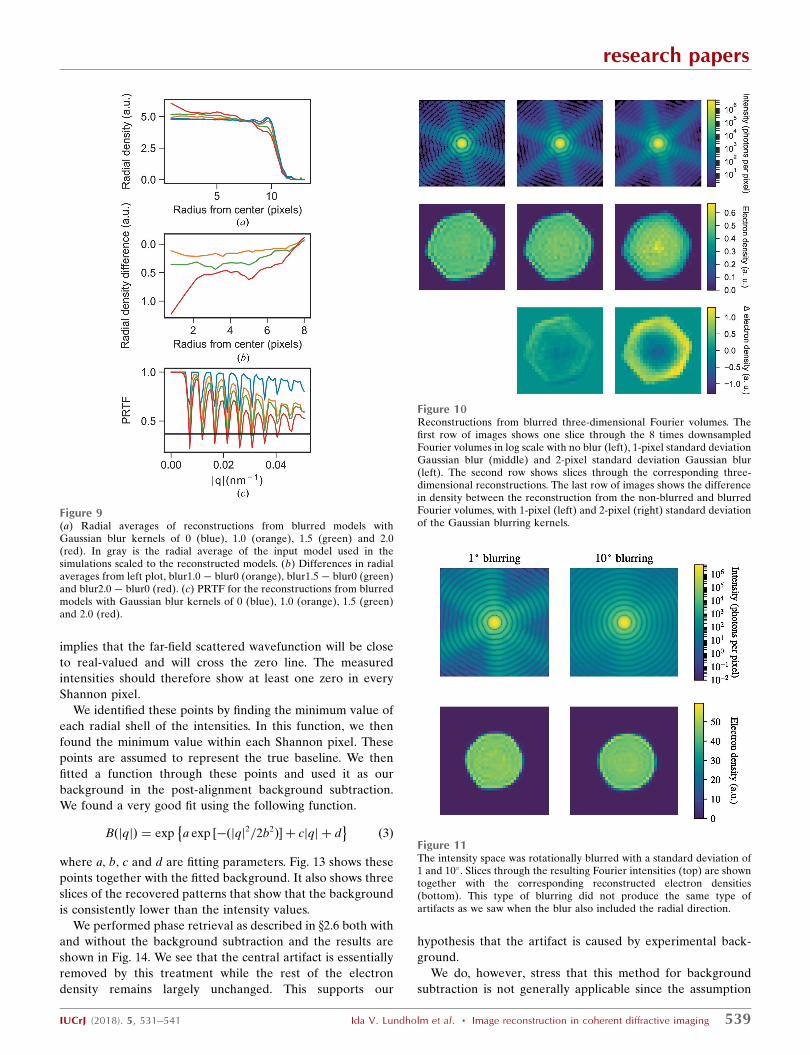
positions (Fig. 9c). The reconstructions from blurred diffrac-

tion volumes show increasing deviation in density from the

non-blurred case. At 1-pixel blur, there is only a slight change

in density which is hardly visible in a two-dimensional slice,

while the reconstruction with 2-pixel blur clearly deviaties

from the input model and has higher density in the center of

the reconstructed object. The difference in density between

the reconstruction from a non-blurred diffraction model and

the blurred models is negative in the center and positive

towards the edge with stronger effects the larger the blurring

(Fig. 10). The average radial-density profiles of the recon-

structions show that blurring in Fourier space causes the

density to be redistributed from the edges to the center (Figs.

9a, 9b and 10). The slope of the density gradient increases with

larger blurring kernels. In the center of the reconstruction a 2-

pixel Gaussian kernel blur introduces a 25% change in density,

a 1.5-pixel blur an 8% change and a 1-pixel blur only around

research papers

IUCrJ (2018). 5, 531–541 Ida V. Lundholm et al. � Image reconstruction in coherent diffractive imaging 537

Figure 7(a) Radial average of three-dimensional reconstructions for experimentaldata with (blue) and without (orange) background subtraction applied onthe raw images. The images show slices through the three-dimensionalreconstructions with background subtraction applied to the raw images(b) and without background subtraction (c).

2% compared with the center of a reconstruction from the

non-blurred Fourier volume. It is clear from these results that

blurring of Fourier space can introduce diffuse artifacts in

reconstructions, an important effect to be evaluated before

interpreting diffuse density changes as real features of biolo-

gical significance (Fig. 10).

Interestingly, we see a similar type of effect from this arti-

ficial blurring as we do in the reconstruction of the experi-

mental data. To distinguish whether this blurring originates

from the data or from the EMC algorithm we applied a second

type of blur. This time we only applied rotational blur, which

simulates the kind of blurring that might be induced by the

EMC algorithm. In Fig. 11 we see that the blurred Fourier

intensity still maintains a high-fringe visibility even at a high

degree of blurring. The reconstructions show no artifact even

for a rotational blur with a standard deviation as high as 10�.

The reconstruction does however, as expected, look signifi-

cantly more spherical. This indicates that the dense artifact in

the experimental data is not caused by the EMC algorithm but

is more likely to be an effect of the experimental background.

3.6. Reconstruction stability

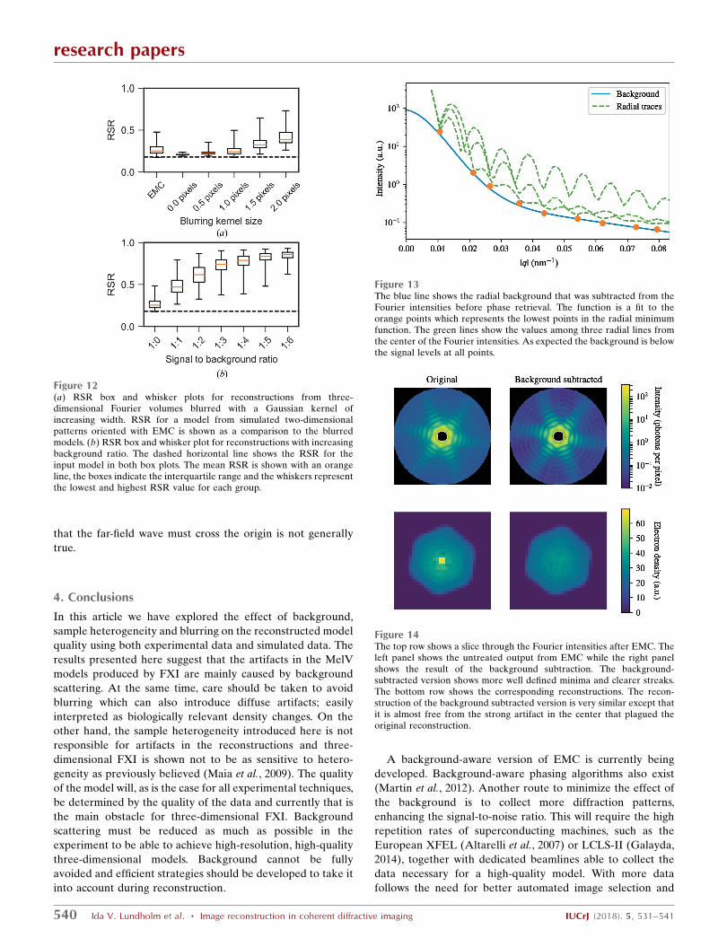
The variation in RSR between individual three-dimensional

images reconstructed from the same Fourier volume can be

used to assess the reconstruction stability. The RSR calculated

here is a measure on how different the reconstructions are

from an object with uniform density, with lower RSR values

indicating high resemblance. A similar RSR for all individual

reconstructions would imply that the Fourier amplitudes given

to the iterative phase retrieval

converges to similar solutions and thus

indicates higher reconstruction stabi-

lity. The capsid and membrane present

in the model particle have higher

density compared with the interior

that increases the total RSR value of

the full particle from 0 to 0.18.

The RSR for reconstruction from a

simulated three-dimensional diffrac-

tion volume is around 0.2 for all indi-

vidual reconstructions. When blurring

is added to the diffraction space, the

RSR variation increases among the

individual reconstructions, which indi-

cates a less stable reconstruction. The

average RSR also increases with

increasing blurring because the indi-

vidual reconstructions are far from

being uniformly dense (Fig. 12). The

RSR analysis shows that the propor-

tion of a reconstruction containing an

artifact and the strength of that artifact

increase together with the standard

deviation of the Gaussian blurring

kernel. The reconstruction from EMC-

oriented simulated patterns is similar

in quality to the reconstruction from a blurred Fourier volume

with a 1-pixel standard deviation Gaussian kernel, both when

it comes to the stability of the reconstructions (high variation

of the RSR) and to the contrast of the reconstructions

(discernible capsid and interior in real-space radial average)

(Fig. 12). This indicates that the impact of blurring in the final

reconstruction should be negligible.

The reconstructions from EMC-oriented patterns with

added experimental background show higher average RSR

the stronger the background. The variance of the RSR

increases only up to a background ratio of 1:4 and then

decreases. For higher background ratios, where EMC has

difficulty converging, the Fourier volume seems to give a more

stable reconstruction (Fig. 12b).

3.7. Post-alignment background subtraction

To further test the hypothesis that the described artifacts

are caused by background scattering we attempted to artifi-

cially remove the background from the aligned Fourier

intensity volume. The background subtraction was done after

the EMC step, since before the EMC step the background is

sparsely sampled, just like the signal, and a background

removal there could cause artifacts such as negative inten-

sities.

We assumed a spherically symmetric background, as

expected from a background dominated by scattering from

residual gas. MelV is an icosahedral virus and is therefore

believed to be close to centrosymmetric and with well-defined

boundaries at the resolution we achieve in this article. This

research papers

538 Ida V. Lundholm et al. � Image reconstruction in coherent diffractive imaging IUCrJ (2018). 5, 531–541

Figure 8(a) Slices through reconstructions from simulated data with experimental background added inincreasing proportions (ratio indicated above each image). (b) The calculated relative density of the 8voxel central artifact compared with the median density of the particle interior for reconstructionswith increasing proportion of experimental background from simulated data using 1000 (orange) and260 (blue) images. (c) The PRTF for the reconstructions.

implies that the far-field scattered wavefunction will be close

to real-valued and will cross the zero line. The measured

intensities should therefore show at least one zero in every

Shannon pixel.

We identified these points by finding the minimum value of

each radial shell of the intensities. In this function, we then

found the minimum value within each Shannon pixel. These

points are assumed to represent the true baseline. We then

fitted a function through these points and used it as our

background in the post-alignment background subtraction.

We found a very good fit using the following function.

BðjqjÞ ¼ exp a exp ½�ðjqj2=2b2Þ þ cjqj þ d� �

ð3Þ

where a, b, c and d are fitting parameters. Fig. 13 shows these

points together with the fitted background. It also shows three

slices of the recovered patterns that show that the background

is consistently lower than the intensity values.

We performed phase retrieval as described in x2.6 both with

and without the background subtraction and the results are

shown in Fig. 14. We see that the central artifact is essentially

removed by this treatment while the rest of the electron

density remains largely unchanged. This supports our

hypothesis that the artifact is caused by experimental back-

ground.

We do, however, stress that this method for background

subtraction is not generally applicable since the assumption

research papers

IUCrJ (2018). 5, 531–541 Ida V. Lundholm et al. � Image reconstruction in coherent diffractive imaging 539

Figure 9(a) Radial averages of reconstructions from blurred models withGaussian blur kernels of 0 (blue), 1.0 (orange), 1.5 (green) and 2.0(red). In gray is the radial average of the input model used in thesimulations scaled to the reconstructed models. (b) Differences in radialaverages from left plot, blur1.0 � blur0 (orange), blur1.5 � blur0 (green)and blur2.0 � blur0 (red). (c) PRTF for the reconstructions from blurredmodels with Gaussian blur kernels of 0 (blue), 1.0 (orange), 1.5 (green)and 2.0 (red).

Figure 10Reconstructions from blurred three-dimensional Fourier volumes. Thefirst row of images shows one slice through the 8 times downsampledFourier volumes in log scale with no blur (left), 1-pixel standard deviationGaussian blur (middle) and 2-pixel standard deviation Gaussian blur(left). The second row shows slices through the corresponding three-dimensional reconstructions. The last row of images shows the differencein density between the reconstruction from the non-blurred and blurredFourier volumes, with 1-pixel (left) and 2-pixel (right) standard deviationof the Gaussian blurring kernels.

Figure 11The intensity space was rotationally blurred with a standard deviation of1 and 10�. Slices through the resulting Fourier intensities (top) are showntogether with the corresponding reconstructed electron densities(bottom). This type of blurring did not produce the same type ofartifacts as we saw when the blur also included the radial direction.

that the far-field wave must cross the origin is not generally

true.

4. Conclusions

In this article we have explored the effect of background,

sample heterogeneity and blurring on the reconstructed model

quality using both experimental data and simulated data. The

results presented here suggest that the artifacts in the MelV

models produced by FXI are mainly caused by background

scattering. At the same time, care should be taken to avoid

blurring which can also introduce diffuse artifacts; easily

interpreted as biologically relevant density changes. On the

other hand, the sample heterogeneity introduced here is not

responsible for artifacts in the reconstructions and three-

dimensional FXI is shown not to be as sensitive to hetero-

geneity as previously believed (Maia et al., 2009). The quality

of the model will, as is the case for all experimental techniques,

be determined by the quality of the data and currently that is

the main obstacle for three-dimensional FXI. Background

scattering must be reduced as much as possible in the

experiment to be able to achieve high-resolution, high-quality

three-dimensional models. Background cannot be fully

avoided and efficient strategies should be developed to take it

into account during reconstruction.

A background-aware version of EMC is currently being

developed. Background-aware phasing algorithms also exist

(Martin et al., 2012). Another route to minimize the effect of

the background is to collect more diffraction patterns,

enhancing the signal-to-noise ratio. This will require the high

repetition rates of superconducting machines, such as the

European XFEL (Altarelli et al., 2007) or LCLS-II (Galayda,

2014), together with dedicated beamlines able to collect the

data necessary for a high-quality model. With more data

follows the need for better automated image selection and

research papers

540 Ida V. Lundholm et al. � Image reconstruction in coherent diffractive imaging IUCrJ (2018). 5, 531–541

Figure 12(a) RSR box and whisker plots for reconstructions from three-dimensional Fourier volumes blurred with a Gaussian kernel ofincreasing width. RSR for a model from simulated two-dimensionalpatterns oriented with EMC is shown as a comparison to the blurredmodels. (b) RSR box and whisker plot for reconstructions with increasingbackground ratio. The dashed horizontal line shows the RSR for theinput model in both box plots. The mean RSR is shown with an orangeline, the boxes indicate the interquartile range and the whiskers representthe lowest and highest RSR value for each group.

Figure 13The blue line shows the radial background that was subtracted from theFourier intensities before phase retrieval. The function is a fit to theorange points which represents the lowest points in the radial minimumfunction. The green lines show the values among three radial lines fromthe center of the Fourier intensities. As expected the background is belowthe signal levels at all points.

Figure 14The top row shows a slice through the Fourier intensities after EMC. Theleft panel shows the untreated output from EMC while the right panelshows the result of the background subtraction. The background-subtracted version shows more well defined minima and clearer streaks.The bottom row shows the corresponding reconstructions. The recon-struction of the background subtracted version is very similar except thatit is almost free from the strong artifact in the center that plagued theoriginal reconstruction.

classification procedures, where machine learning with deep

neural networks may provide a powerful tool.

Funding information

This work was supported by the Swedish Research Council,

the Knut and Alice Wallenberg Foundation, the European

Research Council, the Swedish Foundation for Strategic

Research, the Rontgen-Angstrom Cluster, the Swedish

Foundation for International Cooperation in Research and

Higher Education, the Czech Ministry of Education, Youth

and Sports as part of targeted support from the National

Programme of Sustainability II, the Chalmers Area of

Advance: Materials Science, ELIBIO (CZ.02.1.01/0.0/0.0/

15_003/0000447) from the European Regional Development

Fund, Advanced research using high intensity laser produced

photons and particles (ADONIS) (CZ.02.1.01/0.0/0.0/16_019/

0000789) from the European Regional Development Fund,

the Volkswagen foundation, the Panofsky fellowship from

SLAC, the US Department of Energy, Office of Basic Energy

Sciences, Division of Chemical Sciences, Geosciences, and

Biosciences through Argonne National Laboratory under

contract DE-AC02-06CH11357 and NKFIH K115504. We are

grateful to the scientific and technical staff of the Linac

Coherent Light Source (LCLS) for support. Use of the LCLS,

SLAC National Accelerator Laboratory, is supported by the

US Department of Energy, Office of Science, Office of Basic

Energy Sciences under Contract No. DE-AC0276SF00515.

Data were collected in July 2014 as part of proposal LC69.

References

Altarelli, M. et al. (2007). The European X-ray Free-Electron Laser.Technical Design Report 2006-097. DESY, Hamburg, Germany.

Barty, A., Kirian, R. A., Maia, F. R. N. C., Hantke, M., Yoon, C. H.,White, T. A. & Chapman, H. (2014). J. Appl. Cryst. 47, 1118–1131.

Bergh, M., Huldt, G., Tımneanu, N., Maia, F. R. N. C. & Hajdu, J.(2008). Q. Rev. Biophys. 41, 181–204.

Bozek, J. D. (2009). Eur. Phys. J. Spec. Top. 169, 129–132.Chapman, H. N., Barty, A., Bogan, M. J. et al. (2006). Nat. Phys. 2,

839–843.Chapman, H. N., Barty, A., Marchesini, S. et al. (2006). J. Opt. Soc.

Am. A, 23, 1179–200.

Daurer, B. J., Hantke, M. F., Nettelblad, C. & Maia, F. R. N. C. (2016).J. Appl. Cryst. 49, 1042–1047.

Daurer, B. J. et al. (2017). IUCrJ, 4, 251–262.Ekeberg, T. et al. (2015). Phys. Rev. Lett. 114, 098102.Emma, P. et al. (2010). Nat. Photonics, 4(9), 641–647.Ferguson, K. R. et al. (2015). J. Synchrotron Rad. 22, 492–497.Fienup, J. R. (1978). Opt. Lett. 3, 27–29.Galayda, J. N. (2014). The linac coherent light source-II project.

Technical Report, SLAC National Accelerator Laboratory, MenloPark, USA.

Gorkhover, T. et al. (2018). Nat. Photonics, 12, 150–153.Hantke, M. F., Ekeberg, T. & Maia, F. R. N. C. (2016). J. Appl. Cryst.

49, 1356–1362.Hantke, M. F. et al. (2014). Nat. Photonics, 8, 943–949.Huldt, G., Szoke, A. & Hajdu, J. (2003). J. Struct. Biol. 144,

219–227.Jones, T. A., Zou, J.-Y., Cowan, S. W. & Kjeldgaard, M. (1991). Acta

Cryst. A47, 110–119.Jurek, Z., Faigel, G. & Tegze, M. (2004). Eur. Phys. J. D. At. Mol. Opt.

Phys. 29, 217–229.Kassemeyer, S. et al. (2012). Opt. Express, 20, 4149.Kurta, R. P. et al. (2017). Phys. Rev. Lett. 119, 158102.Loh, N. D. et al. (2010). Phys. Rev. Lett. 104, 225501.Loh, N. D. & Elser, V. (2009). Phys. Rev. E, 80, 026705.Luke, D. R. (2005). Inverse Probl. 21, 37–50.Maia, F. R., Ekeberg, T., Tımneanu, N., van der Spoel, D. & Hajdu, J.

(2009). Phys. Rev. E, 80, 031905.Maia, F. R. N. C., Ekeberg, T., van der Spoel, D. & Hajdu, J. (2010). J.

Appl. Cryst. 43, 1535–1539.Mancuso, A. P. et al. (2010). New J. Phys. 12, 035003.Marchesini, S., He, H., Chapman, H. N., Hau-Riege, S. P., Noy, A.,

Howells, M. R., Weierstall, U. & Spence, J. C. (2003). Phys. Rev. B,68, 140101.

Martin, A. V. et al. (2012). Opt. Express, 20, 16650–16661.Neutze, R., Wouts, R., van der Spoel, D., Weckert, E. & Hajdu, J.

(2000). Nature, 406, 752–757.Okamoto, K., Miyazaki, N., Reddy, H. K., Hantke, M. F., Maia, F. R.,

Larsson, D. S., Abergel, C., Claverie, J. M., Hajdu, J., Murata, K. &Svenda, M. (2018). Virology, 516, 239–245.

Rickwood, D. (1978). Centrifugal separations in molecular and cellbiology, edited by G. D. Birnie and D. Rickwood, p. 219. London:Information Retrieval Ltd.

Schot, G. van der, et al. (2015). Nat. Commun. 6, 5704.Seibert, M. M. et al. (2010). J. Phys. B At. Mol. Opt. Phys. 43, 194015.Seibert, M. M. et al. (2011). Nature, 470, 78–81.Sellberg, J. A. et al. (2014). Nature, 510, 381–384.Spence, J. C. (2017). IUCrJ, 4, 322–339.Struder, L. et al. (2010). Nucl. Instrum. Methods Phys. Res. A, 614,

483–496.

research papers

IUCrJ (2018). 5, 531–541 Ida V. Lundholm et al. � Image reconstruction in coherent diffractive imaging 541