RESEARCH REPORT SERIES (Statistics #2014-02) · RESEARCH REPORT SERIES (Statistics #2014-02) Modeling the Effects of Recent Field Interventions . in the National Crime Victimization

RESEARCH REPORT SERIES (Statistics #2014-02)

Modeling the Effects of Recent Field Interventions in the National Crime Victimization Survey

Joseph L. Schafer

Center for Statistical Research & Methodology Research and Methodology Directorate

U.S. Census Bureau Washington, D.C. 20233

Report Issued: April 3, 2014 Disclaimer: This report is released to inform interested parties of research and to encourage discussion. The views expressed are those of the authors and not necessarily those of the U.S. Census Bureau.

Modeling the Effects of Recent Field Interventionsin the National Crime Victimization SurveyResearch Report Series (Statistics)Joseph L. SchaferMarch 2014RRS2014-02

Disclaimer. This report is released to informinterested parties of research and to encouragediscussion. The views expressed are those of theauthor and not necessarily those of the U.S.Census Bureau.

1 BACKGROUND

The National Crime Victimization Survey (NCVS) isa household-based demographic survey that yieldsannual national estimates of property crime andnonfatal violent crime, both reported and notreported to the police. Interviews are conductedyear-round by Census Bureau Field Representatives(FRs) through personal visit or by telephone, usinga Computer-Assisted Personal Interview (CAPI)instrument. In sampled households, persons ofage 12 and older are given screener interviews todetermine if they have been victimized during theprevious six months. If a crime is reported duringthe screener, the interview continues with anincident report to ascertain details of the event.

In 2012, NCVS field staff experienced two majorinterventions that may have affected data quality.

First, a program of refresher training and enhancedperformance monitoring, which had begun in late2011, was continued and completed in 2012. Thistraining reoriented FRs to the purpose of the NCVSand reinforced the importance of following correctprocedures, especially during screener interviews.After the training, supervisors began to monitor FRperformance using an expanded set of data qualityindicators. This program was phased in by anexperiment. Teams of FRs were randomly assignedto two cohorts. One cohort received the programin late 2011, and the other received it in early2012. More details of the program and therandomization procedure are given in Section 2. Bythe beginning of the second quarter of 2012, over98% of the experienced NCVS interviewers had

HIGHLIGHTS

NCVS field staff experienced two majorinterventions in 2012: completion of a refreshertraining and performance monitoring programwhich began the previous year, and a fieldrealignment effort which reduced the number ofCensus Bureau Regional Offices from twelve tosix. To assess the impact of these interventions,we fit Bayesian longitudinal models describingkey quality indicators and survey outcomes overa five-year period (2008–2012). After accountingfor long-term trends, annual periodic cycles,characteristics of the interviewers’ monthlyassignments, and random interviewer variation,we detected some statistically significant effectsof the interventions on the following variables.

• Response rates: Refresher training andperformance monitoring were associatedwith a modest but significant decrease inhousehold response rates in 2011 but notin 2012.

• Screener times: Refresher training andperformance monitoring produced largeand significant increases in the averageduration of the screener interview in 2011and 2012.

• Personal crime and household propertycrime: Neither the refresher training andperformance monitoring program nor fieldrealignment were associated with anysignificant changes in the collection ofcrimes in 2012.

Because no significant effects on the collectionof crimes were detected, there is no evidence tosuggest that victimization rates for 2012 orcomparisons between 2012 and previous yearswere impacted.

U.S. Department of CommerceEconomics and Statistics AdministrationU.S. CENSUS BUREAUcensus.gov

completed the training, and the performancemonitoring system was in place for all FRs. For theremainder of the year, newly hired FRs weretrained as they entered the NCVS workforce andput on the enhanced monitoring program.

Second, field operations for NCVS and all otherCensus Bureau surveys were consolidated fromtwelve Regional Offices (ROs) to six. This so-calledfield realignment was phased in during 2012. Bythe end of the year, six ROs had closed, and fieldstaff from these closing ROs were reassigned.

In this report, we present new longitudinal analysesof quality indicators and survey outcomes. Thedata come from approximately 1,900 FRs, 420,000attempted household interviews and 750,000personal contacts over the five-year period from2008 to 2012. Our immediate goal is tocharacterize the effects of refresher training,performance monitoring and field realignment, toinform us of any potential impact of theseinterventions on victimization estimates for 2012and comparisons to previous years. More broadly,these models provide a new methodologicalframework for understanding temporal patternsand trends in the NCVS and other surveys.

Our analyses focus on two key measures of dataquality (household response rate, average durationof the NCVS screener interview) and two key surveyoutcomes (incident rates for personal crimes andhousehold property crimes). In Section 2, wereview the major field interventions that took placein recent years and present graphical summaries ofhow key data-quality and outcome variables havechanged over time. In Section 3, we describe aclass of Bayesian generalized linear mixed modelswith special features that capture the time-varyingaspects of the interventions and the responsevariables. Results for the four outcomes arepresented in Sections 4–7, respectively, followedby discussion of the implications in Section 8.

2 RECENT MAJOR INTERVENTIONSAND TRENDS

Sample Size and Interviewer Workload

The NCVS, and other major demographic surveysconducted by the Census Bureau, uses a complextwo-stage design. The first stage selects PrimarySample Units (PSUs), which are single counties orgroups of counties, and the second stage selectshousing units and group quarters within the PSUs.

Although the same basic design has been usedsince 2006, the size of the survey has changedover time. Beginning in October 2010, the samplesize was boosted by about 25%, reversing somereductions that had been made three years earlier.During this so-called sample reinstatement, thenumber of interviewers was also increased.

A plot of the number of housing units selected forthe NCVS each month from 2008 to 2012 is shownin Figure 1 (a). These figures include units thatwere successfully interviewed and those that werenot, but excludes those that were determined tobe out of scope (e.g., because they were vacant ornot valid residential addresses). Prior to thesample reinstatement in late 2010, the sample sizeremained steady at about 7,000 units per month,and then rose to nearly 9,000 by the secondquarter of 2011. The number of interviewersworking for the NCVS rose over the same period, asshown in Figure 1 (b). The increases in sample sizeand staffing levels nearly offset each other, and theper-interviewer workload remained fairly steadyover time. The distribution of workload (cases perinterviewer per month) at each month is shown bythe boxplots in Figure 1 (c). The median number ofcases per month (represented by each boxplot’scenter line), and the 25th and 75th percentiles(represented by the edges of the boxes), showremarkably little variation over the five-year period.

In this report, we do not attempt to model theeffects of sample reinstatement; those effects, ifpresent, are subsumed into long-term trends andnoise. Nor do we attempt to model the impact ofthe minor changes in interviewer workload overtime. However, the wide variation in workloadwithin any given month suggests a diversity in FRexperiences which may partly explain somevariables of interest. FRs with the highestworkloads (up to 60 cases per month) tend to behighly experienced interviewers who work solelyon the NCVS. FRs with smaller workloads (as few asone case per month) may represent part-timeemployees, or they may work primarily on otherCensus Bureau surveys and receive NCVS casesonly sporadically. Each of the models that we willfit include workload as a covariate. Some of ourmodels will also include it as a denominator for arate or as a precision (inverse-variance) weight.Note that this measure of workload pertains onlyto NCVS; it does not account for work done by theFR for any other Census Bureau surveys. Workloadfor other surveys could not be included in ourmodels because it was not available for the entirefive-year period.

2 | Effects of Field Interventions in the 2012 NCVS

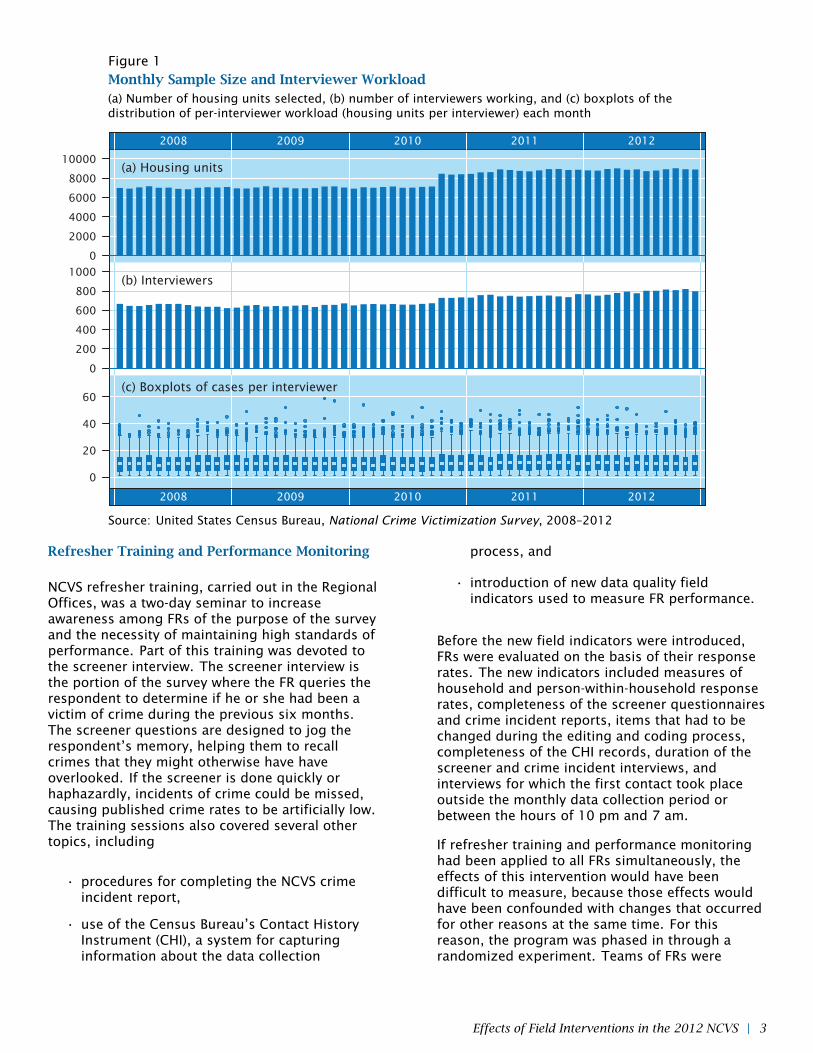
Figure 1Monthly Sample Size and Interviewer Workload(a) Number of housing units selected, (b) number of interviewers working, and (c) boxplots of thedistribution of per-interviewer workload (housing units per interviewer) each month

2008 2009 2010 2011 2012

0

2000

4000

6000

8000

10000(a) Housing units

0

200

400

600

800

1000(b) Interviewers

0

20

40

60(c) Boxplots of cases per interviewer

2008 2009 2010 2011 2012

Source: United States Census Bureau, National Crime Victimization Survey, 2008–2012

Refresher Training and Performance Monitoring

NCVS refresher training, carried out in the RegionalOffices, was a two-day seminar to increaseawareness among FRs of the purpose of the surveyand the necessity of maintaining high standards ofperformance. Part of this training was devoted tothe screener interview. The screener interview isthe portion of the survey where the FR queries therespondent to determine if he or she had been avictim of crime during the previous six months.The screener questions are designed to jog therespondent’s memory, helping them to recallcrimes that they might otherwise have haveoverlooked. If the screener is done quickly orhaphazardly, incidents of crime could be missed,causing published crime rates to be artificially low.The training sessions also covered several othertopics, including

• procedures for completing the NCVS crimeincident report,

• use of the Census Bureau’s Contact HistoryInstrument (CHI), a system for capturinginformation about the data collection

process, and

• introduction of new data quality fieldindicators used to measure FR performance.

Before the new field indicators were introduced,FRs were evaluated on the basis of their responserates. The new indicators included measures ofhousehold and person-within-household responserates, completeness of the screener questionnairesand crime incident reports, items that had to bechanged during the editing and coding process,completeness of the CHI records, duration of thescreener and crime incident interviews, andinterviews for which the first contact took placeoutside the monthly data collection period orbetween the hours of 10 pm and 7 am.

If refresher training and performance monitoringhad been applied to all FRs simultaneously, theeffects of this intervention would have beendifficult to measure, because those effects wouldhave been confounded with changes that occurredfor other reasons at the same time. For thisreason, the program was phased in through arandomized experiment. Teams of FRs were

Effects of Field Interventions in the 2012 NCVS | 3

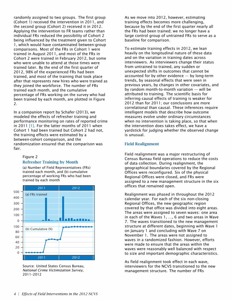
randomly assigned to two groups. The first group(Cohort 1) received the intervention in 2011, andthe second group (Cohort 2) received it in 2012.Applying the intervention to FR teams rather thanindividual FRs reduced the possibility of Cohort 2being influenced by the treatment given to Cohort1, which would have contaminated between-groupcomparisons. Most of the FRs in Cohort 1 weretrained in August 2011, and most of the FRs inCohort 2 were trained in February 2012, but somewho were unable to attend at those times weretrained later. By the end of the first quarter of2012, 98% of the experienced FRs had beentrained, and most of the training that took placeafter that represents new hires who were trained asthey joined the workforce. The number of FRstrained each month, and the cumulativepercentage of FRs working on the survey who hadbeen trained by each month, are plotted in Figure2.

In a companion report by Schafer (2013), wemodeled the effects of refresher training andperformance monitoring on rates of reported crimein 2011 [1]. For the latter months of 2011 whenCohort 1 had been trained but Cohort 2 had not,the training effects were estimated by abetween-cohort comparison, and therandomization ensured that the comparison wasfair.

Figure 2Refresher Training by Month(a) Number of Field Representatives (FRs)trained each month, and (b) cumulativepercentage of working FRs who had beentrained by each month

2011 2012

0

100

200

300

400

500(a) FRs trained

0

20

40

60

80

100(b) Cumulative (%)

2011 2012

Source: United States Census Bureau,National Crime Victimization Survey,2011–2012

As we move into 2012, however, estimatingtraining effects becomes more challenging,because by the end of the first quarter nearly allthe FRs had been trained; we no longer have alarge control group of untrained FRs to serve as abaseline for comparison.

To estimate training effects in 2012, we leanheavily on the longitudinal nature of these dataand on the variation in training dates acrossinterviewers. As interviewers change their statusfrom untrained to trained, any sudden orunexpected shifts in outcomes that cannot beaccounted for by other evidence — by long-termtrends, by seasonal effects that were seen inprevious years, by changes in other covariates, andby random month-to-month variation — will beattributed to training. The scientific basis forinferring causal effects of training is weaker for2012 than for 2011; our conclusions are morecorrelational than causal. These inferences requireintelligent models that describe how outcomemeasures evolve under ordinary circumstanceswhen no intervention is taking place, so that whenthe intervention does takes effect, we have ayardstick for judging whether the observed changeis unusual.

Field Realignment

Field realignment was a major restructuring ofCensus Bureau field operations to reduce the costsof data collection. During realignment, thegeographical boundaries covered by the RegionalOffices were reconfigured. Six of the physicalRegional Offices were closed, and FRs wereassigned to a new management structure in the sixoffices that remained open.

Realignment was phased in throughout the 2012calendar year. For each of the six non-closingRegional Offices, the new geographic regioncovered by that office was divided into eight areas.The areas were assigned to seven waves: one areain each of the Waves 1, …, 6 and two areas in Wave7. The waves transitioned to the new managementstructure at different dates, beginning with Wave 1on January 1 and concluding with Wave 7 onNovember 1. The areas were not assigned towaves in a randomized fashion. However, effortswere made to ensure that the areas within thewaves were reasonably well balanced with respectto size and important demographic characteristics.

As field realignment took effect in each wave,interviewers for the NCVS transitioned to the newmanagement structure. The number of FRs


transitioning each month, and the cumulativepercentage of FRs who had transitioned by eachmonth, are plotted in Figure 3.

To estimate the effects of field realignment, we willfollow a similar strategy as the one we outlined forrefresher training and performance monitoring. Asinterviewers switch over to the new managementstructure, any sudden shift in outcomes thatcannot be explained by long-term trends, seasonaleffects, changes in other covariates, and randommonthly variation will be attributed to realignment.The validity of this approach will depend on theveracity of the model, and its ability to describehow the outcomes evolve under ordinarycircumstances without the intervention.

Two Quality Measures

To assess the effects of refresher training,performance monitoring and field realignment, wewill model two variables that are related to dataquality.

The first quality measure is the NCVS householdresponse rate. This rate is defined as the numberof successful household interviews divided by thenumber of sampled households, excluding theunits determined to be out of scope. A plot of theresponse rate by month for the period 2008–2012

Figure 3Field Realignment by Month(a) Number of Field Representatives (FRs)transitioning each month, and (b)cumulative percentage of working FRs whohad transitioned by each month

2011 2012

0

200

400

600

800(a) FRs transitioning

0

20

40

60

80

100(b) Cumulative (%)

2011 2012


is shown in Figure 4 (a). The response rates wereslowly increasing from 2008 until the first quarterof 2010, and slowly decreasing thereafter. Thispattern may be partly explained by the 2010Decennial Census. The highly visible campaign ofpublic outreach to encourage response to theDecennial Census appears to have had the residualeffect of increasing participation in the NCVS; thisincrease around Census Day (April 1, 2010) andsubsequent decline has been seen in other CensusBureau household surveys as well. Carefulinspection of this plot also suggests the possibilityof annual seasonal effects, such as a dip inresponse rate at the end of each year during theChristmas holiday season. Thus, our efforts tomeasure the effects of refresher training and fieldrealignment take place against a backdrop ofresponse rates that have been steadily decliningfor nearly three years.

The other quality measure is the duration of thescreener interview. A plot of the average monthlyscreener time is shown in Figure 4 (b). Thisvariable sharply increased during late 2011 andearly 2012, during the period of refresher trainingand enhanced performance monitoring. We believethis happened for two reasons. First, a part of thetraining seminar was specifically devoted to thescreener interview, to teaching FRs the importanceof strictly following the protocol of askng all of thescreener questions, even though many of thosequestions seem redundant. Second, the trainingseminar introduced new policies by which themanagers were expected to monitor theperformance of their field staff. Until then, FRs hadbeen graded solely on their response rates.Screener times had averaged less than 90 seconds,and many screeners were over in less than oneminute, suggesting that many FRs were notadministering the screener as designed. Aftertraining, with the implementation of enhancedmonitoring, managers were instructed to useadditional quality measures, including screenertimes, as performance standards. A newbenchmark was set for screener times to be at least3.5 minutes (210 seconds). An increase in screenertime was essentially mandated by a change inmanagement policy. Because the training of FRsand the policy change occurred at approximatelythe same time, it is difficult to separate the effectof FR training from the effect of the policy change.

Two Survey Outcomes

In the sections ahead, we will also examine theeffects of refresher training and field realignmenton two key survey outcomes.


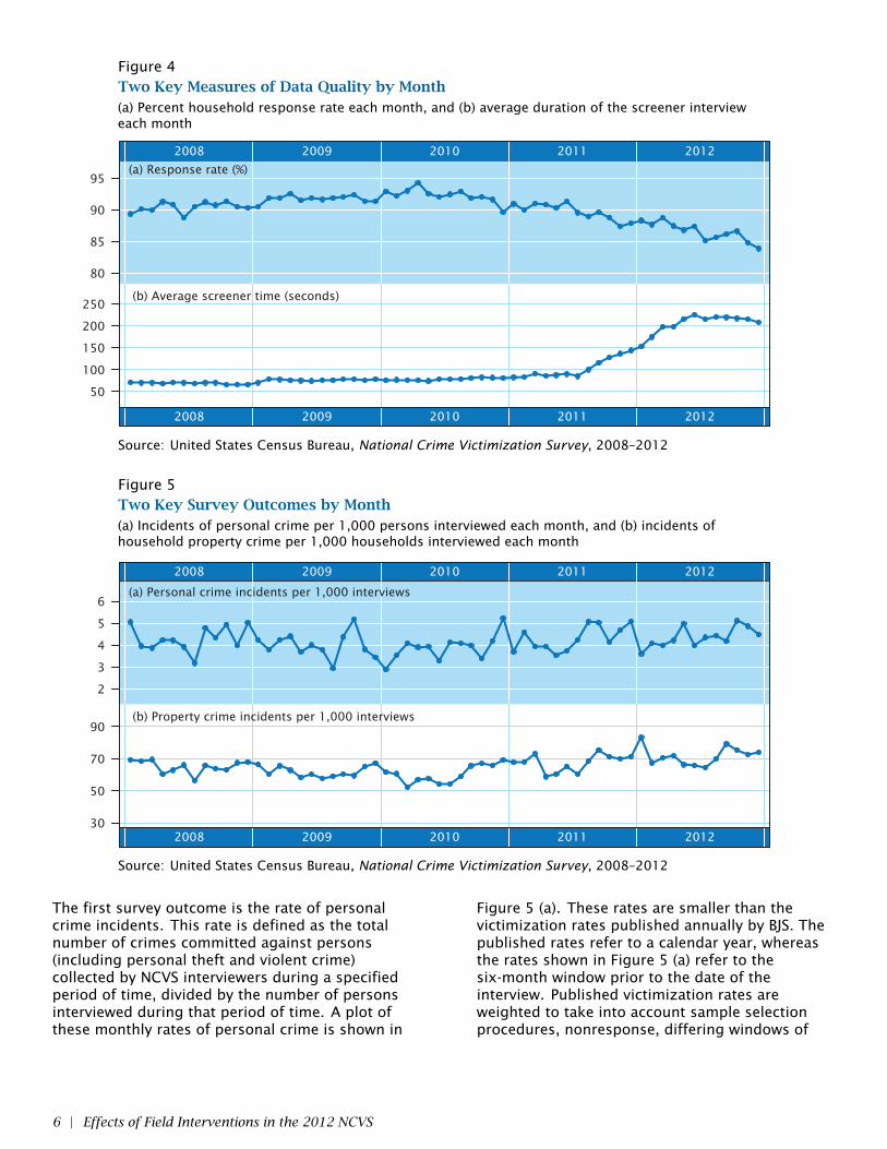
Figure 4Two Key Measures of Data Quality by Month(a) Percent household response rate each month, and (b) average duration of the screener intervieweach month

2008 2009 2010 2011 2012

(a) Response rate (%)

80

85

90

95

50

100

150

200

250(b) Average screener time (seconds)

2008 2009 2010 2011 2012


Figure 5Two Key Survey Outcomes by Month(a) Incidents of personal crime per 1,000 persons interviewed each month, and (b) incidents ofhousehold property crime per 1,000 households interviewed each month

2008 2009 2010 2011 2012

(a) Personal crime incidents per 1,000 interviews

2

3

4

5

6

30

50

70

90(b) Property crime incidents per 1,000 interviews

2008 2009 2010 2011 2012


The first survey outcome is the rate of personalcrime incidents. This rate is defined as the totalnumber of crimes committed against persons(including personal theft and violent crime)collected by NCVS interviewers during a specifiedperiod of time, divided by the number of personsinterviewed during that period of time. A plot ofthese monthly rates of personal crime is shown in

Figure 5 (a). These rates are smaller than thevictimization rates published annually by BJS. Thepublished rates refer to a calendar year, whereasthe rates shown in Figure 5 (a) refer to thesix-month window prior to the date of theinterview. Published victimization rates areweighted to take into account sample selectionprocedures, nonresponse, differing windows of


time, and the fact that some crimes have multiplevictims. Nevertheless, the two measures areclosely related, and changes in the rates shown inFigure 5 (a) will strongly affect the published rates.The rates shown in Figure 5 (a) are generally risingfrom 2010 to 2012, with fluctuations due topossible seasonal effects and noise.

Our second survey outcome is the rate ofhousehold property crime incidents. This variable,plotted in Figure 5 (b), is the number of householdproperty crimes collected by interviewers dividedby the number of households interviewed. Thisrate also appears to rise from 2010 to 2012, withpossible seasonal effects and noise.

Our previous analyses showed that refreshertraining and enhanced monitoring increased theapparent rates of personal crime and householdproperty crime during the latter months of 2011,but only among those crimes that had not beenreported to police [1]. In the sections ahead, wewill again distinguish crimes by whether or notthey were reported to police. For certain categoriesof crime, unreported crimes tend to be less seriousand harder for respondents to recall. Crimesreported to police may be more salient inrespondents’ memories and more likely to bereported to FRs during the screener interviews,whereas unreported crimes may be less salient andmore susceptible to interviewer effects andchanges in the field conditions. Relationshipsbetween salience and difficulty of recall have beendemonstrated by Miller and Groves (1985) [2] andby Czaja et al. (1994) [3].

3 MODELING STRATEGY

Basic Form of the Models

The variables plotted in Figures 4 and 5 aresummary measures for each month. But theinterventions of interest, refreshertraining/performance monitoring and fieldrealignment, took effect in different months fordifferent FRs. This variation in timing across FRs isa key part of our strategy for estimatingintervention effects. In a sense, this variation intiming across FRs provides the replication that weneed to separate the effects of the interventionfrom long-term trends and seasonal shifts thatmay be happening at the same time. To tease outthe effects of interventions from other temporalphenomena, we must disaggregate the data byinterviewers. The basic unit of analysis for each ofour models is the interviewer-month.

Measurements for interviewer-months are severelyunbalanced. From 2008 to 2012, the number ofinterviewers working for the NCVS in any givenmonth was approximately 650–800. Over theentire period, however, about 1,900 differentinterviewers worked on the survey. Some highlyexperienced FRs were present for all five years, butmany worked on the survey only sporadically, andsome were present for only a single month.Methods that require a complete or nearlycomplete series for each interviewer will not beappropriate for these data. Fortunately, the modelsthat we fit are not adversely affected by the lack ofbalance. Each interviewer contributes observationsfor however many months he or she worked for theNCVS from 2008 to 2012, and where appropriate,each month’s contribution is weighted by theinterviewer’s NCVS caseload during that month.

Each of our models will take the following generalform. Let Yij denote an aggregated outcome (e.g.,response rate) for interviewer i during month tj .We assume that

Yij ∼ F (µij ; ϕ,wij), (1)

where F is a user-specified parametric family withmean µij = E (Yij), optional dispersion parameter ϕ,and optional inverse-variance weight wij . The meanis decomposed as

g(µij) = ωij + f1( tj ) + f2( tj ) + αi + xTij β, (2)

where

• g is a user-specified link function,

• ωij is an optional offset term needed for ratemodels,

• f1 is a smooth function describing a long-termtrend,

• f2 is a periodic function describing an annualcycle,

• αi is a random effect for interviewer i ,assumed to be distributed as N(0,σ2

α),

• xij is a vector of covariates, and

• β is a vector of coefficients to be estimated.

The effects of field interventions are contained inβ, and their interpretation will depend on how thevariables in xij are coded. The reliability of thoseestimates will depend on how accurately wedescribe the long-term and annual trends in f1 andf2. For our purposes, it is best to avoid simple


parametric forms (e.g., linear or quadraticfunctions of time) which are probably unrealistic,and work with function classes that are moregeneral. Before listing the covariates in xij , wedescribe our strategy for characterizing f1 and f2.

Approximating a Long-Term Trend Using aNatural Cubic Spline

Splines are classes of functions that are flexibleenough to approximate a trend of almost anyshape. To introduce the idea, suppose that wehave a data series y1, ... , yn that represents aresponse variable recorded at times t1, ... , tn.Suppose that

yi = f (ti ) + ϵi ,

where the ϵi ’s are independent errors with meanzero and constant variance. Our goal is to estimatef , a function that is believed to be continuous andsmooth but whose shape is not otherwise known.To create a spline, we first partition the real lineinto K + 1 intervals,

(−∞, ξ1) , [ξ1, ξ2), ... , [ξK ,∞).

where the cutpoints ξ1 < ξ2 < · · · < ξK are calledknots. A spline of degree r consists of an rthdegree polynomial over each interval,

f (t) =

β00 + β01 t + ... + β0r t

r if t ∈ (−∞, ξ1),β10 + β11 t + ... + β1r t

r if t ∈ [ξ1, ξ2),...

βK0 + βK1 t + ... + βKr tr if t ∈ [ξK ,∞).

To make the function continuous and smooth, wewill apply constraints to the β’s to force f and itsfirst r − 1 derivatives to be continuous at the knots.Various methods for constructing splines areavailable. One simple method relies on thetruncated power basis. In this method, a spline ofdegree r with knots at ξ1, ... , ξK is written as

f (t) = β0 + β1 t + · · · + βr tr

+ u1 (t − ξ1)r+ + · · · + uK (t − ξK )

r+,

where

(t − ξj)r+ =

{(t − ξj)

r if t ≥ ξj ,0 otherwise.

To estimate f , we compute the r + K + 1 basisfunctions

1, t, ... , tr , (t − ξ1)r+, ... , (t − ξK )

r+

for t1, ... , tn and treat them as regressors, fitting anordinary least-squares (OLS) regression of y1, ... , ynon these variables to estimate the β’s and u’s. If alinear regression is not appropriate (e.g., if the yirepresents a proportion or rate) then we can easily

switch to a generalized linear model (e.g., logisticor loglinear regression).

To illustrate, Figure 6 shows an artificial dataset ofn = 26 observations whose measurement times areequally spaced. The line plotted in Figure 6 (a) is acubic spline with K = 5 equally spaced knots fit byOLS. Cubic splines are a popular choice, becausethey are very smooth; the knots in the fitted curveare invisible to the eye. One disadvantage shownby this example is that at the ends of the series,the fitted function becomes erratic; beyond theboundary knots (where t < ξi and t > ξk ), theestimate of f (t) is strongly pulled toward the firstand last observations (y1 and yn), causing the curveto veer off in implausible directions.

To stabilize a cubic spline near the edges of thespace, it is customary to impose additionalconstraints to require the function to be linearbeyond the boundary knots,

f ′′(t) = 0 for t ≤ ξ1 and t ≥ ξK .

A cublic spline with this constraint is called anatural cubic spline. Natural cubic splines can beconstructed in various ways. For our purposes, wewill use second divided differences of truncatedpower functions (White et al., 1998; Welham,2008) [4] [5]. Given a set of knots ξ1, ... , ξk , thenatural cubic spline is written as

f (t) = β0 + β1 t +K−1∑k=2

uk P∗k (t),

where

P∗k (t) =

16

{h−1k (t − ξk+1)

3+ − (h−1

k + h−1k−1 ) (t − ξk)

3+

+ h−1k−1 (t − ξk−1)

3+

},

and hk = (ξk+1 − ξk). To reduce collinearity, wereplace P∗

k (t) with

Pk(t) = P∗k (t) − ak − bk t,

where ak and bk are the intercept and slope fromthe ordinary least-squares regression of P∗

k (t) on tover the sample points,[

ak

bk

]=

[n

∑ni=1 ti∑n

i=1 ti∑n

i=1 t2i

]−1 [ ∑ni=1 P

∗k (ti )∑n

i=1 ti P∗k (ti )

].

The basis becomes

f (t) = β0 + β1 t +

K−1∑k=2

uk Pk(t). (3)

This representation has the attractive property that

uk = f ′′(ξk)


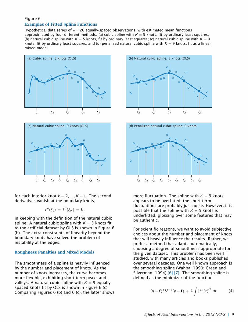
Figure 6Examples of Fitted Spline FunctionsHypothetical data series of n = 26 equally-spaced observations, with estimated mean functionsapproximated by four different methods: (a) cubic spline with K = 5 knots, fit by ordinary least squares;(b) natural cubic spline with K = 5 knots, fit by ordinary least squares; (c) natural cubic spline with K = 9knots, fit by ordinary least squares; and (d) penalized natural cubic spline with K = 9 knots, fit as a linearmixed model

(a) Cubic spline, 5 knots (OLS) (b) Natural cubic spline, 5 knots (OLS)

(c) Natural cubic spline, 9 knots (OLS) (d) Penalized natural cubic spline, 9 knots

ξ1 ξ2 ξ3 ξ4 ξ5 ξ1 ξ2 ξ3 ξ4 ξ5

ξ1 ξ2 ξ3 ξ4 ξ5 ξ6 ξ7 ξ8 ξ9 ξ1 ξ2 ξ3 ξ4 ξ5 ξ6 ξ7 ξ8 ξ9

for each interior knot k = 2, ... ,K − 1. The secondderivatives vanish at the boundary knots,

f ′′(ξ1) = f ′′(ξK ) = 0,

in keeping with the definition of the natural cubicspline. A natural cubic spline with K = 5 knots fitto the artificial dataset by OLS is shown in Figure 6(b). The extra constraints of linearity beyond theboundary knots have solved the problem ofinstability at the edges.

Roughness Penalties and Mixed Models

The smoothness of a spline is heavily influencedby the number and placement of knots. As thenumber of knots increases, the curve becomesmore flexible, exhibiting short-term peaks andvalleys. A natural cubic spline with K = 9 equallyspaced knots fit by OLS is shown in Figure 6 (c).Comparing Figures 6 (b) and 6 (c), the latter shows

more fluctuation. The spline with K = 9 knotsappears to be overfitted; the short-termfluctuations are probably just noise. However, it ispossible that the spline with K = 5 knots isunderfitted, glossing over some features that maybe authentic.

For scientific reasons, we want to avoid subjectivechoices about the number and placement of knotsthat will heavily influence the results. Rather, weprefer a method that adapts automatically,choosing a degree of smoothness appropriate forthe given dataset. This problem has been wellstudied, with many articles and books publishedover several decades. One well known approach isthe smoothing spline (Wahba, 1990; Green andSilverman, 1994) [6] [7]. The smoothing spline isdefined as the minimizer of the function

(y − f)TV−1(y − f) + λ

∫[f ′′(t)]

2dt (4)


over the space of twice-differentiable functions f ,where y = (y1, ... , yn)

T , f = ( f (t1), ... , f (tn) )T , V is the

covariance matrix of Y1, ... ,Yn, and λ is auser-specified smoothing parameter. The solutionto this minimization problem is a natural cubicspline with knots located at the design points (i.e.,at all the distinct values of ti ).

Smoothing splines have attractive theoreticalproperties, but computing them becomes timeconsuming as the number of design pointsincreases. An economical alternative is to specify agrid of knots, spaced equally over the range oft1, ... , tn or at their quantiles, and fit a spline with aroughness penalty. Variations on this approach areknown as P-splines (Eilers and Marx, 1996) [8] andpenalized splines (Ruppert, Wand and Carroll,2003) [9].

Consider a natural cubic spline model

yi = β0 + β1 ti +K−1∑k=2

uk Pk(ti ) + ϵi ,

where ϵi ∼ N(0,σ2ϵ ), and where the Pk ’s are the

basis functions shown in (3). Suppose we apply alarge number of knots ξ1, ... , ξK spaced at regularintervals. The number of knots is not crucial,provided that it is large enough that the ordinaryregression estimate will be overfitted. Estimatingthe β’s and u’s by OLS will produce a fitted curvethat exhibits too much fluctuation. However, if wetreat the u’s as random variables drawn from acommon distribution,

u2, ... , uK−1 ∼ N(0,σ2u), (5)

then we can estimate the additional variancecomponent σ2

u from the data. The model becomes

y = Xβ + Pu + ϵ, (6)

where

X =

1 t11 t2...

...1 tn

, P =

P2(t1) ... PK−1(t1)P2(t2) ... PK−1(t2)

.... . .

...P2(tn) ... PK−1(tn)

,

β = (β0,β1)T , u = (u2, u3, ... , uk−1)

T , andϵ = (ϵ1, ϵ2, ... , ϵn)

T , and where

u ∼ N(0,σ2u I),

ϵ ∼ N(0,σ2ϵV).

This is an example of a linear mixed model, alsoknown as a linear mixed-effects model. It differsfrom common examples of linear mixed models in

that the observational units j = 1, ... , n are crossedwith the random coefficients rather than nestedwithin them. Nevertheless, this model can be fitwith software packages that accommodate crossedrandom effects (e.g., PROC MIXED in SAS).Estimates of the random coefficients in u will beshrunk toward zero, producing a curve that issmoother than the OLS version. In fact, underthese basis functions, the uj ’s represent thesecond derivatives of f at the interior knots, andthe distributional assumption on u imposes aroughness penalty that is a discrete approximationto the second term in the smoothing spline (4).The fitted curve from this penalized natural cubicspline is a data-determined compromise betweenthe overfitted OLS spline and a simple linearregression of y1, ... , yn on t1, ... , tn.

To illustrate, we fit a penalized natural cubic splinewith K = 9 knots to the artificial dataset shown inFigure 6, using the linear mixed-model formulation(6). The resulting curve is plotted in Figure 6 (d).The extra distributional assumption (5) imposedon the u’s has effectively removed the short-termpeaks and valleys found in the OLS curve of Figure6 (c).

In the following way, we embed penalized naturalcubic splines into our models for NCVS data.Returning to the model shown in Equation (2), werepresent the long-term trend as

f1(t) = β0 + β1 t +K−1∑k=2

uk Pk(t), (7)

with knots ξ1, ... , ξK placed at the beginning of eachquarter-year. The first two regressors (the constantand t) are placed into the covariate vector xij , sothat β0 and β1 are subsumed into β. The basisfunctions P2(t), ... ,PK−1(t) are added to the model(2) as regressors with random coefficientsdistributed as u2, ... , uK−1 ∼ N(0,σ2

u). The resultingmodel becomes a generalized linear mixed modelwith observational units that are crossed with therandom coefficients u2, ... , uK−1.

Approximating a periodic trend by a periodiccubic spline

In addition to the long-term trend f1, we need amethod for specifying the function f2 in our model(2) that is both flexible and periodic, with a periodfixed at one year. That is, if t is expressed inyears, we need f2(t) to be continuous and smooth,with the property

f2(t) = f2(t + 1) = f2(t + 2) = · · ·

for any value of t.


Various methods for incorporating periodic trendsinto longitudinal models have been proposed. Onepopular technique is to apply a Fourier basisconsisting of sine-cosine pairs. Using a Fourierbasis, a periodic function with period T can beexpressed as

f2(t) =

M∑m=1

{δ2m−1 sin

(2πmt

T

)+ δ2m cos

(2πmt

T

)},

where δ1, ... , δ2M are coefficients to be estimated.With monthly measurements, we have 12− 1 = 11degrees of freedom available to estimate an annualcycle, so the largest number of sine-cosine pairswe can use is M = 5. While experimenting withFourier bases, we found that the resulting fittedfunction f2 exhibited implausible short-termoscillations within the year. To dampen theseshort-term oscillations, we switched to a methodbased on periodic cubic splines (Zhang, Lin andSowers, 2000) [10].

To construct a periodic spline with period T , webegin with the ordinary cubic spline

f2(t) = β0 + β1 t + β2 t2 + β3 t

3 +K∑

k=1

δj (t − ξj)3+ (8)

for coefficients β0, ... ,β3, δ1, ... , δK , with knotslocated between 0 and T . To make the splineperiodic over t ∈ [0,∞), two changes are needed.First, we replace each occurrence of t on theright-hand side of (8) with the seasonal operator

s(t) = mod(t,T ).

Second, we enforce continuity upon f and its firsttwo derivatives by imposing the constraintsf2(0) = f2(T ), f ′2(0) = f ′2(T ), and f ′′2 (0) = f ′′(T ). Withsome algebra, the constrained version of (8)becomes

f2(t) = β0 +K∑

k=1

δk P∗k ( s(t) ),

where

P∗k (s) = aks + bks

2 + cks3 + (s − ξk)

3+,

and

ak = − T (T − ξk)

2+

3(T − tk)2

2− (T − ξk)

3

T,

bk =3(T − ξk)

2− 3(T − ξk)

2

2T,

ck = − T − ξkT

,

which corrects a typographical error by Zhang, Linand Sowers (2000) [10]. Finally, we impose anadditional requirement that∫

f2(t) dt ≈ 0

by setting β0 = 0 and centering each basis functionat its average value, averaging over the designpoints of t. Let t1, t2, ... , tn denote the distinctvalues of t appearing in the dataset, and let

Pk(s) = P∗k (s) − Pk ,

where

Pk =1

n

n∑i=1

P∗k ( s(ti ) ).

The function becomes

f2(t) =

K∑k=1

ξk Pk( s(t) ).

We found that by placing K = 6 knots over thecalendar year at two-month intervals, we have beenable capture the major features of each periodictrend, but without the implausible within-yearoscillations that were an artifact of the Fourierbasis. These six periodic basis functions are placedin the covariate vector xij of our model (2), and thecorresponding coefficients are subsumed into β.

Intervention Effects

Having described the long-term and periodictrends, we now turn our attention to the effects ofthe interventions. After experimenting withdifferent ways to code the interventions, we settledon a very simple method. To account for refreshertraining and performance monitoring, we created apair of dummy indicators,

After.Training.2011ij = 1 if tj is in 2011 andinterviewer i had beentrained, 0 otherwise,

After.Training.2012ij = 1 if tj is in 2012 andinterviewer i had beentrained, 0 otherwise,

and included them as covariates in the vector xij .The corresponding elements of β become simplecontrasts (trained minus untrained) for 2011 and2012.

Similarly, we defined a dummy indicator for fieldrealignment,

After.Realignmentij = 1 if interviewer iexperienced realignmentby month tj , 0 otherwise,


so that the corresponding element of β is a simplecontrast (realigned versus not).

Information for estimating these coefficientscomes mainly from data in late 2011 and 2012when the interventions are being phased in. Datafrom earlier years may strengthen these estimatesby providing information about long-term andperiodic trends and the effects of other covariates.

Additional Covariates

In addition to the long-term and periodic trends,our models include additional covariates to adjustfor differences in the interviewers’ monthlyassignments. One key covariate, which wedescribed in Section 2, is the interviewer’scaseload,

WLHHij = number of NCVS HH’s assigned tointerviewer i during month tj .

In each of our models, this variable is included as acovariate in xij . Depending on the model, it mayalso appear as a precision weight wij or as an offsetterm ωij .

The other covariate in our models comes from theCensus Bureau’s Planning Database. The PlanningDatabase, which was created using data from the2010 Census and the American Community Survey,provides information at fine levels of geography(census block groups) that are known to be helpfulfor planning and designing surveys. One suchvariable is a national classification of block-groupsinto three clusters that represent different levels ofdifficulty for conducting census and surveyoperations. Cluster 1 represents areas whereenumeration is easy and response rates tend to behigh. Rural and suburban locations tend to fall intoCluster 1. Clusters 2 and 3 represent more heavilyurbanized areas where data collection tends to bemore difficult. By linking to the Planning Database,we were able to identify the cluster membershipfor about 88% of the housing units in NCVS. Forthe remaining 12%, the cluster could not bedetermined because key geographic informationwas missing. Exploratory analyses showed thatamong those 12%, the NCVS response rates wereunusually low, so we decided to combine themwith Clusters 2 and 3. We then aggregated thisvariable to produce a summary statistic for theinterviewer-month,

Cluster.1ij = proportion of interviewer i ’scases during month tjthat are known to belong toPlanning Database Cluster 1.

We conjectured that this covariate would have asignificant positive correlation with response ratesand a significant negative correlation to crimerates.

Fitting the Models

The models we have described are generalizedlinear mixed models with an unusual pattern ofcrossed and nested random effects. Althoughsome existing software packages (PROC NLMIXEDin SAS, the GLAMM package in Stata) are capable offitting models like these, we could not find anyavailable package that had all the capabilities weneeded. With observations for approximately42,000 interviewer-months, it is difficult to fitthese models in a reasonable amount of time.

To compute parameter estimates, we implementeda specialized Bayesian Markov chain Monte Carlo(MCMC) procedure programmed in Fortran 95 andcalled from R. For each model, the MCMC chainwas run for 25,000 cycles following a burn-inperiod of 1,000 cycles. Parameters weresubsampled and saved with a thinning interval of 5cycles, yielding a sample of 5,000 draws from theposterior distribution.

For an overview of the algorithm and the priordistributions applied to the parameters, see theTechnical Appendix by Schafer (2013) [1].

4 RESULTS FOR HOUSEHOLD RESPONSERATES

In our first model, the outcome variable is

Yij = household response rate forinterviewer i during month tj .

We assumed a binomial distribution,

Yij ∼ n−1ij Bin( nij , µij),

where nij = WLHHij is the number of householdsassigned to interviewer i during month tj . The linkfunction is logistic, and the mean function is

log(

µij

1− µij

)= f1(tj) + f2(tj) + αi + xTij β,

where f1 is a long-term trend, f2 is an annualperiodic cycle, αi is a random effect for intervieweri , xij is a vector of covariates, and β is a vector ofcoefficients.

The estimate of the long-term trend is plotted inFigure 7 (a), along with pointwise 95% error


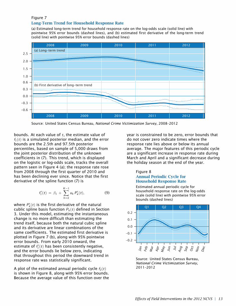
Figure 7Long-Term Trend for Household Response Rate(a) Estimated long-term trend for household response rate on the log-odds scale (solid line) withpointwise 95% error bounds (dashed lines), and (b) estimated first derivative of the long-term trend(solid line) with pointwise 95% error bounds (dashed lines)

2008 2009 2010 2011 2012

(a) Long-term trend

1.0

1.5

2.0

2.5

(b) First derivative of long-term trend

-0.6

-0.3

0.0

0.3

0.6

2008 2009 2010 2011 2012


bounds. At each value of t, the estimate value off1(t) is a simulated posterior median, and the errorbounds are the 2.5th and 97.5th posteriorpercentiles, based on sample of 5,000 draws fromthe joint posterior distribution of the unknowncoefficients in (7). This trend, which is displayedon the logistic or log-odds scale, tracks the overallpattern seen in Figure 4 (a); the response rate rosefrom 2008 through the first quarter of 2010 andhas been declining ever since. Notice that the firstderivative of the spline function (7) is

f ′1(t) = β1 +

K−1∑k=2

uk P′k(t), (9)

where P ′k(t) is the first derivative of the natural

cublic spline basis function Pk(t) defined in Section3. Under this model, estimating the instantaneouschange is no more difficult than estimating thetrend itself, because both the natural cubic splineand its derivative are linear combinations of thesame coefficients. The estimated first derivative isplotted in Figure 7 (b), along with 95% pointwiseerror bounds. From early 2010 onward, theestimate of f ′1(t) has been consistently negative,and the error bounds lie below zero, indicatingthat throughout this period the downward trend inresponse rate was statistically significant.

A plot of the estimated annual periodic cycle f2(t)is shown in Figure 8, along with 95% error bounds.Because the average value of this function over the

year is constrained to be zero, error bounds thatdo not cover zero indicate times where theresponse rate lies above or below its annualaverage. The major features of this periodic cycleare a significant increase in response rate duringMarch and April and a significant decrease duringthe holiday season at the end of the year.

Figure 8Annual Periodic Cycle forHousehold Response RateEstimated annual periodic cycle forhousehold response rate on the log-oddsscale (solid line) with pointwise 95% errorbounds (dashed lines)

Q1 Q2 Q3 Q4

-0.2

-0.1

0.0

0.1

0.2

Jan

Feb

Mar

Apr

May

Jun

Jul

Aug

Sep

Oct

Nov

Dec



Table 1: Coefficients, standard errors, andBayesian p-values from model forhousehold response rate

Coef SE p

WLHH .0011 .0009 .224

Cluster.1 .0682 .0240 .004

After.Training.2011 −.0847 .0335 .014

After.Training.2012 −.0677 .0390 .078

After.Realignment .0760 .0459 .096

Source: United State Census Bureau,National Crime Victimization Survey, 2008–2012

Estimates for the key coefficients in β are shown inTable 1, along with standard errors and simulatedp-values. In this table and all subsequent tables,the estimated coeffients and standard errors aresimulated posterior means and standarddeviations, averaged across 5,000 random drawsfrom the Bayesian posterior distribution. Thep-values are simulated Bayesian p-values, definedas one minus the probability content of thenarrowest equal-tailed posterior interval thatcovers the parameter’s null value of zero. Thesemay be interpreted in roughly the same manner assignificance values from frequentist two-tailedhypothesis tests, with a value of .05 or lessindicating an effect that is statistically significant.

In Table 1, the coefficient for WLHH (.0011) is notsignificantly different from zero (p = .224),indicating that there is little evidence of arelationship between response rates andinterviewers’ monthly workloads.

The coefficient for Cluster.1 (.0682) is positive andstatistically significant (p = .004). As expected, ahigher proportion of households located inPlanning Database Cluster 1 is associated with ahigher response rate.

Examining the coefficient for After.Training.2011(−.0847), we see that the estimated effect ofrefresher training and performance monitoring in2011 is negative and statistically significant(p = .014). The corresponding effect for 2012((−.0677)) is not significant (p = .078). Thesecoefficients pertain to the log-odds. To understandthe implications on the probability scale, supposewe start with a response rate of 90%. A change inthe log-odds of −0.0847 would reduce the rate by0.8 percentage points to 89.2%, and a change inthe log-odds of −0.0677 reduces the rate by 0.6percentage points to 89.4%. Thus, refreshertraining and performance monitoring areassociated with a modest but significant decrease

in household response rates in 2011, and asmaller, non-significant decrease in 2012.

One possible explanation for why refreshertraining and performance monitoring would reduceresponse rates is the change in perfomancestandards that were discussed in Section 2. Priorto training, FRs were evaluated solely on theirresponse rates. As the interviewers were trained,managers were instructed to begin monitoringtheir performance by additional quality measuresthat included screener times. If FRs had previouslybeen trying to convert difficult cases (householdsfor which response was unlikely) by conducting thescreeners too quickly, then we would expectresponse rates under the new performancemeasures to go down. The fact that they havegone down only slightly is relatively good news. Itseems plausible that the new measures had theintended consequence of emphasizing surveyquality over just response rates, possibly reducingfalsified and quick interviews.

The estimated coefficient for After.Realignment(.0760) is positive. Field realignment wasimplemented during 2012, a period whenresponse rates were declining. If this effect werereal, it would indicate that realignment slowed thatdecline, and the response rate after realignmentwas slightly higher (by approximately 0.7percentage points) than it would have beenwithout realignment. However, this effect is notstatistically significant (p = .096), so the evidencefor an effect of realignment is inconclusive.

5 RESULTS FOR SCREENER TIMES

For our second model, the response variable is

Yij = average screener time forinterviewer i during month tj .

We assumed a normal distribution,

Yij ∼ N(µij , σ2/nij ),

where nij is the number of persons interviewed byinterviewer i during month tj . The link function isthe identity. Preliminary analyses revealed thatthere were no discernible annual periodic effects inscreener times, so we simplified this model byremoving the periodic component. The model is

µij = f1(tj) + αi + xTij β,

where f1 is a long-term trend, αi is a random effectfor interviewer i , xij is a vector of covariates, and βis a vector of coefficients.


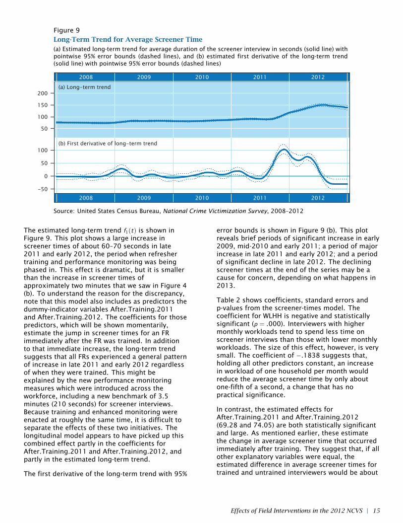
Figure 9Long-Term Trend for Average Screener Time(a) Estimated long-term trend for average duration of the screener interview in seconds (solid line) withpointwise 95% error bounds (dashed lines), and (b) estimated first derivative of the long-term trend(solid line) with pointwise 95% error bounds (dashed lines)

2008 2009 2010 2011 2012

(a) Long-term trend

50

100

150

200


-50

0

50

100

2008 2009 2010 2011 2012


The estimated long-term trend f1(t) is shown inFigure 9. This plot shows a large increase inscreener times of about 60–70 seconds in late2011 and early 2012, the period when refreshertraining and performance monitoring was beingphased in. This effect is dramatic, but it is smallerthan the increase in screener times ofapproximately two minutes that we saw in Figure 4(b). To understand the reason for the discrepancy,note that this model also includes as predictors thedummy-indicator variables After.Training.2011and After.Training.2012. The coefficients for thosepredictors, which will be shown momentarily,estimate the jump in screener times for an FRimmediately after the FR was trained. In additionto that immediate increase, the long-term trendsuggests that all FRs experienced a general patternof increase in late 2011 and early 2012 regardlessof when they were trained. This might beexplained by the new performance monitoringmeasures which were introduced across theworkforce, including a new benchmark of 3.5minutes (210 seconds) for screener interviews.Because training and enhanced monitoring wereenacted at roughly the same time, it is difficult toseparate the effects of these two initiatives. Thelongitudinal model appears to have picked up thiscombined effect partly in the coefficients forAfter.Training.2011 and After.Training.2012, andpartly in the estimated long-term trend.

The first derivative of the long-term trend with 95%

error bounds is shown in Figure 9 (b). This plotreveals brief periods of significant increase in early2009, mid-2010 and early 2011; a period of majorincrease in late 2011 and early 2012; and a periodof significant decline in late 2012. The decliningscreener times at the end of the series may be acause for concern, depending on what happens in2013.

Table 2 shows coefficients, standard errors andp-values from the screener-times model. Thecoefficient for WLHH is negative and statisticallysignificant (p = .000). Interviewers with highermonthly workloads tend to spend less time onscreener interviews than those with lower monthlyworkloads. The size of this effect, however, is verysmall. The coefficient of −.1838 suggests that,holding all other predictors constant, an increasein workload of one household per month wouldreduce the average screener time by only aboutone-fifth of a second, a change that has nopractical significance.

In contrast, the estimated effects forAfter.Training.2011 and After.Training.2012(69.28 and 74.05) are both statistically significantand large. As mentioned earlier, these estimatethe change in average screener time that occurredimmediately after training. They suggest that, if allother explanatory variables were equal, theestimated difference in average screener times fortrained and untrained interviewers would be about


Table 2: Coefficients, standard errors, andBayesian p-values from model foraverage screener time

Coef SE p

WLHH −.1838 .0390 .000

Cluster.1 −.9582 1.137 .392

After.Training.2011 69.28 1.798 .000

After.Training.2012 74.05 2.384 .000

After.Realignment 3.538 2.849 .214


70 seconds. Over the same period of time whentraining was taking place, however, the long-termtrend showed an average increase of roughly60-70 seconds. Taken together, these effectsaccount for an increase in average screener timesby about two minutes that were seen in late 2011and early 2012 as refresher training and enhancedmonitoring were being phased in.

6 RESULTS FOR PERSONAL CRIME

Our next model describes the number of incidentsof personal crime recorded during the interviewprocess. The response variable is

Yij = personal crimes discovered byinterviewer i during month tj .

This variable is assumed to have a negativebinomial distribution,

Yij ∼ NegBin(α = κ−1, β = κ−1µij ),

where κ > 0 is an unknown dispersion parameter.We applied a negative binomial model becausepreliminary analyses showed that the responseswere overdispersed relative to a Poissondistribution.

It is reasonable to believe that the number ofpersonal crimes reported by an interviewer isapproximately proportional to the number ofpersons interviewed. That is, we may suppose

µij ∝ nij ,

where nij is the number of persons interviewed byinterviewer i during month tj . Applying thisassumption, and using a logarithmic link, themodel for the mean becomes

logµij = ωij + f1(tj) + f2(tj) + αi + xTij β,

where ωij = log nij , f1(t) and f2(t) are long-term andperiodic trends, αi is a random effect forinterviewer i , and xij is a vector of covariates. Theωij on the right-hand side of the equation is calledan offset term; it is a predictor whose coefficient isassumed to be fixed at one. Alternatively, we canplace the offset to the left-hand side, so that thiscan be viewed as a loglinear model for thepersonal crime incident rate,

log(µij

nij

)= f1(tj) + f2(tj) + αi + xTij β. (10)

Plots of the estimated long-term trend ft(t), andthe estimated first derivative of the estimatedlong-term trend f ′1(t), are shown in Figure 10. Theestimate of f1(t) shows a mild decrease from 2008to 2010 and a mild increase from 2010 to 2012.Except for a period in 2009 where the errorbounds on f ′1(t) briefly dip below zero, theevidence for change is not conclusive. However,the overall pattern is consistent with the officialvictimization estimates reported annually by BJS.Except for small numbers of personal thefts(pocket picking, completed or attempted pursesnatching), most of the crime incidents included inthis model were classified as violent crimes.Truman, Langton and Planty (2013) reported thatrates of violent crime victimization rose over thelast two years (from 2010 to 2011, and from 2011to 2012) after a period of steady decline prior to2010 [11]. The curve shown in Figure 10 (a) hasthe same shape: declining from 2008 to 2010,rising from 2010 to 2012.

A plot of the estimated annual periodic cycle f2(t) isshown in Figure 11. The only feature of this cyclethat is statistically significant is a slight dip aroundthe month of July; during the rest of the calendaryear, the rate of personal crime incidents is notsignificantly different from the annual average.

Estimated coefficients, standard errors andp-values from this model are shown in Table 3.The coefficient for WLHH is small (−.0014) and notsignificantly different from zero (p = .495)). As weconjectured, the coefficient for Cluster.1 (−.2295)is negative and significant (p = .000). Interviewerswhose assignments include a higher proportion ofhousing units in Cluster 1 tend to report fewerincidents of personal crime. The coefficient forAfter.Realignment is small (−.0527) andinsignificant (p = .614), so there is no evidencethat the field realignment program of 2012affected the collection of personal crimes.


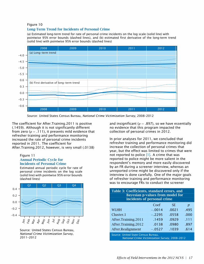
Figure 10Long-Term Trend for Incidents of Personal Crime(a) Estimated long-term trend for rate of personal crime incidents on the log scale (solid line) withpointwise 95% error bounds (dashed lines), and (b) estimated first derivative of the long-term trend(solid line) with pointwise 95% error bounds (dashed lines)

2008 2009 2010 2011 2012

(a) Long-term trend

-5.5

-5.0

-4.5

-4.0


-0.6

-0.3

0.0

0.3

0.6

2008 2009 2010 2011 2012


The coefficient for After.Training.2011 is positive(.1459). Although it is not significantly differentfrom zero (p = .111), it presents mild evidence thatrefresher training and performance monitoringincreased the rate of personal crime incidentsreported in 2011. The coefficient forAfter.Training.2012, however, is very small (.0138)

Figure 11Annual Periodic Cycle forIncidents of Personal CrimeEstimated annual periodic cycle for rate ofpersonal crime incidents on the log scale(solid line) with pointwise 95% error bounds(dashed lines)

Q1 Q2 Q3 Q4

-0.4

-0.2

0.0

0.2

0.4

Jan

Feb

Mar

Apr

May

Jun

Jul

Aug

Sep

Oct

Nov

Dec


and insignificant (p = .897), so we have essentiallyno evidence that this program impacted thecollection of personal crimes in 2012.

In prior analyses for 2011, we concluded thatrefresher training and performance monitoring didincrease the collection of personal crimes thatyear, but the effect was limited to crimes that werenot reported to police [1]. A crime that wasreported to police might be more salient in therespondent’s memory and more easily discoveredby an FR during a screener interview, whereas anunreported crime might be discovered only if theinterview is done carefully. One of the major goalsof refresher training and performance monitoringwas to encourage FRs to conduct the screener

Table 3: Coefficients, standard errors, andBayesian p-values from model forincidents of personal crime

Coef SE p

WLHH −.0014 .0021 .495

Cluster.1 −.2295 .0558 .000

After.Training.2011 .1459 .0929 .111

After.Training.2012 .0138 .0980 .897

After.Realignment −.0527 .1039 .614



Table 4: Coefficients, standard errors and Bayesian p-values from model for incidents of personal crime,classified by by whether the crime was reported to police

All personal crimes Reported to police Not reported to police

Coef SE p Coef SE p Coef SE p

WLHH −.0014 .0021 .495 −.0007 .0024 .782 −.0029 .0028 .306

Cluster.1 −.2295 .0558 .000 −.1987 .0663 .003 −.2568 .0757 .001

After.Training.2011 .1459 .0929 .111 .0224 .1178 .832 .2948 .1271 .018

After.Training.2012 .0138 .0980 .897 −.0707 .1201 .581 .0976 .1309 .456

After.Realignment −.0527 .1309 .614 −.0975 .1242 .423 .0292 .1374 .829


more carefully. Therefore, if this program had animpact on the collection of crimes, it is reasonableto think that the effect would be stronger forcrimes that were less salient.

To see if our present analyses support a similarconclusion, we applied the current model (10) justto personal crimes that were reported to police,and again to personal crimes that were notreported to police. Coefficients, standard errorsand p-values from these separate models areshown in Table 4. For crimes reported to police,the coefficient for After.Training.2011 is small(.0224) and insignificant (p = .832), but for crimesnot reported to police, the coefficient is large(.2948) and significant (p = .018). Thus, theresults for 2011 shown here are highly consistentwith what we found in our previous analyses [1].

However, these effects of training and monitoringappear to have been short-lived. The coefficientsfor After.Training.2012 shown in Table 4 are smalland insignificant. The elevation in personal crimesdue to training and monitoring seen in late 2011was apparently not sustained into 2012.

7 RESULTS FOR PROPERTY CRIME

Our final model describes incidents of householdproperty crime. The response variable is

Yij = household property crimes discovered byinterviewer i during month tj .

As in our previous model, we assume

Yij ∼ NegBin(α = κ−1, β = κ−1µij ),

where κ is a dispersion parameter. The offset is

ωij = log nij ,

where nij is the number of household interviewsconducted by interviewer i during month tj . In all

other respects, this model has the same form asthe previous one (10). The estimated long-termtrend and its first derivative are plotted in Figure12. A mild but statistically significant decline tookplace in 2008 and 2009, but from 2010 onwardthe trend is essentially flat. According to officialnational estimates published by BJS, however, therate of property crime victimization rose between2010 and 2011 and between 2011 and 2012, andboth increases were statistically significant [11][12]. We can think of several possible explanationsfor this apparent discrepancy. First, the nationalestimates were weighted to adjust for the sampledesign, nonresponse and other complications,whereas the model that generated the trends inFigure 12 was applied to raw, unweighted surveyresponses. Second, the national estimatesrepresent marginal rates, whereas the trendsshown in Figure 12 condition upon sometime-varying covariates. Third, the estimatedcurves in Figure 12 contain a fair amount of noise;in particular, the error bounds on the firstderivative are wide enough that we cannot rule outthe possibility that the rate may have increasedfrom 2010 to 2012. Although the shape of thetrends in Figure 12 do not closely mimic the trendin national estimates, the discrepancy is not largeenough to be worrisome.

The estimated annual periodic cycle for householdproperty crime is shown in Figure 13. Rates aresignificantly higher than the annual average duringthe holiday season of late November throughJanuary, and significantly lower than the annualaverage during May, June and July.

Table 5 shows estimated coefficients, standarderrors and p-values from the property-crimemodel. As in the personal-crime model, thecoefficient for WLHH is close to zero (.0022) andinsignificant (p = .086), whereas the effect ofCluster.1 is negative (−.1907) and highlysignificant (p = .000). As we conjectured, a higher


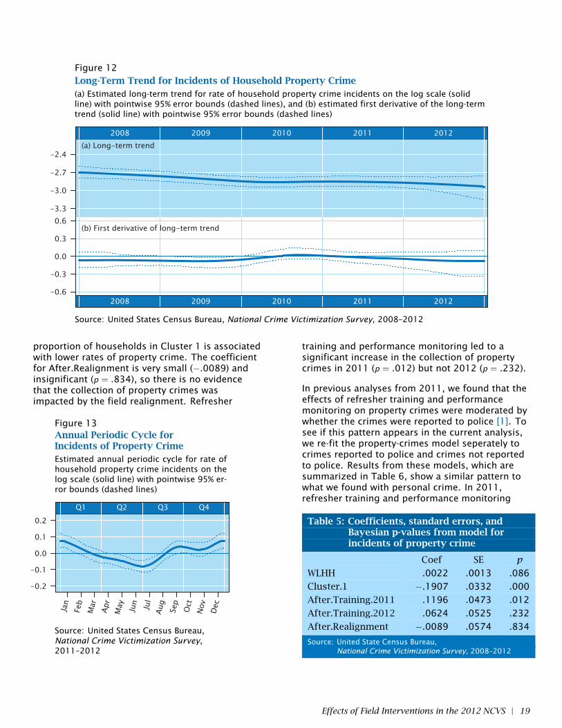
Figure 12Long-Term Trend for Incidents of Household Property Crime(a) Estimated long-term trend for rate of household property crime incidents on the log scale (solidline) with pointwise 95% error bounds (dashed lines), and (b) estimated first derivative of the long-termtrend (solid line) with pointwise 95% error bounds (dashed lines)

2008 2009 2010 2011 2012

(a) Long-term trend

-3.3

-3.0

-2.7

-2.4


-0.6

-0.3

0.0

0.3

0.6

2008 2009 2010 2011 2012


proportion of households in Cluster 1 is associatedwith lower rates of property crime. The coefficientfor After.Realignment is very small (−.0089) andinsignificant (p = .834), so there is no evidencethat the collection of property crimes wasimpacted by the field realignment. Refresher

Figure 13Annual Periodic Cycle forIncidents of Property CrimeEstimated annual periodic cycle for rate ofhousehold property crime incidents on thelog scale (solid line) with pointwise 95% er-ror bounds (dashed lines)

Q1 Q2 Q3 Q4

-0.2

-0.1

0.0

0.1

0.2

Jan

Feb

Mar

Apr

May

Jun

Jul

Aug

Sep

Oct

Nov

Dec


training and performance monitoring led to asignificant increase in the collection of propertycrimes in 2011 (p = .012) but not 2012 (p = .232).

In previous analyses from 2011, we found that theeffects of refresher training and performancemonitoring on property crimes were moderated bywhether the crimes were reported to police [1]. Tosee if this pattern appears in the current analysis,we re-fit the property-crimes model seperately tocrimes reported to police and crimes not reportedto police. Results from these models, which aresummarized in Table 6, show a similar pattern towhat we found with personal crime. In 2011,refresher training and performance monitoring

Table 5: Coefficients, standard errors, andBayesian p-values from model forincidents of property crime

Coef SE p

WLHH .0022 .0013 .086

Cluster.1 −.1907 .0332 .000

After.Training.2011 .1196 .0473 .012

After.Training.2012 .0624 .0525 .232

After.Realignment −.0089 .0574 .834



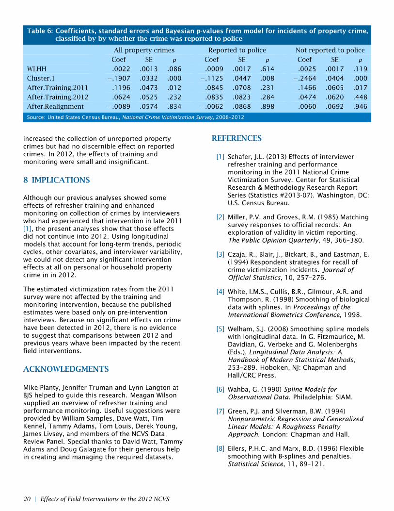
Table 6: Coefficients, standard errors and Bayesian p-values from model for incidents of property crime,classified by by whether the crime was reported to police

All property crimes Reported to police Not reported to police

Coef SE p Coef SE p Coef SE p

WLHH .0022 .0013 .086 .0009 .0017 .614 .0025 .0017 .119

Cluster.1 −.1907 .0332 .000 −.1125 .0447 .008 −.2464 .0404 .000

After.Training.2011 .1196 .0473 .012 .0845 .0708 .231 .1466 .0605 .017

After.Training.2012 .0624 .0525 .232 .0835 .0823 .284 .0474 .0620 .448

After.Realignment −.0089 .0574 .834 −.0062 .0868 .898 .0060 .0692 .946


increased the collection of unreported propertycrimes but had no discernible effect on reportedcrimes. In 2012, the effects of training andmonitoring were small and insignificant.

8 IMPLICATIONS

Although our previous analyses showed someeffects of refresher training and enhancedmonitoring on collection of crimes by interviewerswho had experienced that intervention in late 2011[1], the present analyses show that those effectsdid not continue into 2012. Using longitudinalmodels that account for long-term trends, periodiccycles, other covariates, and interviewer variability,we could not detect any significant interventioneffects at all on personal or household propertycrime in in 2012.

The estimated victimization rates from the 2011survey were not affected by the training andmonitoring intervention, because the publishedestimates were based only on pre-interventioninterviews. Because no significant effects on crimehave been detected in 2012, there is no evidenceto suggest that comparisons between 2012 andprevious years whave been impacted by the recentfield interventions.

ACKNOWLEDGMENTS

Mike Planty, Jennifer Truman and Lynn Langton atBJS helped to guide this research. Meagan Wilsonsupplied an overview of refresher training andperformance monitoring. Useful suggestions wereprovided by William Samples, Dave Watt, TimKennel, Tammy Adams, Tom Louis, Derek Young,James Livsey, and members of the NCVS DataReview Panel. Special thanks to David Watt, TammyAdams and Doug Galagate for their generous helpin creating and managing the required datasets.

REFERENCES

[1] Schafer, J.L. (2013) Effects of interviewerrefresher training and performancemonitoring in the 2011 National CrimeVictimization Survey. Center for StatisticalResearch & Methodology Research ReportSeries (Statistics #2013-07). Washington, DC:U.S. Census Bureau.

[2] Miller, P.V. and Groves, R.M. (1985) Matchingsurvey responses to official records: Anexploration of validity in victim reporting.The Public Opinion Quarterly, 49, 366–380.

[3] Czaja, R., Blair, J., Bickart, B., and Eastman, E.(1994) Respondent strategies for recall ofcrime victimization incidents. Journal ofOfficial Statistics, 10, 257–276.

[4] White, I.M.S., Cullis, B.R., Gilmour, A.R. andThompson, R. (1998) Smoothing of biologicaldata with splines. In Proceedings of theInternational Biometrics Conference, 1998.

[5] Welham, S.J. (2008) Smoothing spline modelswith longitudinal data. In G. Fitzmaurice, M.Davidian, G. Verbeke and G. Molenberghs(Eds.), Longitudinal Data Analysis: AHandbook of Modern Statistical Methods,253–289. Hoboken, NJ: Chapman andHall/CRC Press.

[6] Wahba, G. (1990) Spline Models forObservational Data. Philadelphia: SIAM.

[7] Green, P.J. and Silverman, B.W. (1994)Nonparametric Regression and GeneralizedLinear Models: A Roughness PenaltyApproach. London: Chapman and Hall.

[8] Eilers, P.H.C. and Marx, B.D. (1996) Flexiblesmoothing with B-splines and penalties.Statistical Science, 11, 89–121.


[9] Ruppert, D., Wand, M.P. and Carrol, R.J.(2003) Semiparametric Regression. NewYork: Cambridge University Press.

[10] Zhang, D., Lin, X. and Sowers, M.F. (2000)Semiparametric regression for periodiclongitudinal hormone data from multiplemenstrual cycles. Biometrics, 56, 31–39.

[11] Truman, J., Langton, L. and Planty, M. (2013)Criminal Victimization, 2012. U.S.Department of Justice, Bureau of JusticeStatistics, NCJ 243389, October 2013.

[12] Truman, J. and Planty, M. (2012) CriminalVictimization, 2011. U.S. Department ofJustice, Bureau of Justice Statistics, NCJ239437, October 2012.


Documents

RESEARCH REPORT SERIES (Statistics #2014-02) · RESEARCH REPORT SERIES (Statistics #2014-02) Modeling the Effects of Recent Field Interventions . in the National Crime Victimization