Reservoir characterization using oil-production-induced microseismicity,Clinton County, Kentucky

James T. Rutledge, Nambe Geophysical, Inc., jrutledge@lanl.gov

W. Scott Phillips, Nambe Geophysical, Inc., wsp@lanl.gov

Barbra K. Schuessler, Los Alamos National Laboratory, schuess@seismo5.lanl.gov

LA-UR 96-3066

Submitted to Tectonophysics September 9, 1996.

Accepted April 7, 1997.

Issued: Tectonophysics289 (1998) 129-152.

Text and figures can be accessed at: http://www.ees4.lanl.gov/microeq

Los Alamos National LaboratoryGeoEngineering Group / EES-4

Mail Stop D443Los Alamos, NM 87545

USA

-1-

eld,

600

erived

t rate;

a have

ed

ts or

essure

tal oil

vals

the

gle

area,

iated

thrust

slight

essure

tive

ction-

Abstract

Microseismic monitoring tests were conducted from 1993 to 1995 in the Seventy-Six oil fi

Clinton County, Kentucky. Oil is produced from low-porosity, fractured carbonate rocks at <

m depth. Downhole geophones were deployed in wells located within 120 to 250 m of new

production wells. Three tests were conducted sequentially for 91/2, 201/2, and 30 week periods

during which 110, 180 and 3237 microearthquakes were detected, respectively. Moment-d

magnitudes ranged from -2.5 to 0.9. Volumes extracted ranged from about 1300 to 1800 m3; no

injection operations were conducted. Gross changes in production rate correlate with even

event rate lags changes in production rate by 2 to 3 weeks. Hypocenters and first-motion dat

revealed previously undetected, low-angle thrust faults above and below the currently-drain

depth intervals. Production history, well logs and drill tests indicate the seismically-active faul

fractures are previously-drained intervals that have subsequently recovered to hydrostatic pr

via brine invasion. Storage capacity computed for one of these drained fractures implies to

production represents about 20% of total pore volume. Correlation of older production inter

and well-log porosity anomalies with the seismically-active faults indicate the oil reservoir in

study area is primarily a set of compartmentalized, low-angle thrust faults. Although low-an

fracture sets have not previously been considered in the exploration and development of the

the mapped thrust faults are consistent with other investigators’ interpretations of oil assoc

with secondary fracture sets occurring along deeper-seated, wrench-fault structures.

Stress determined from composite focal mechanisms indicates a near-surface (<550 m)

regime. Maximum horizontal stress direction is N15°W ±15°, rotated approximately 90° from

regional orientation. The seismic behavior is consistent with poroelastic models that predict

increases in horizontal compressive stress above and below currently-drained volumes. Pr

re-equilibration via brine invasion replacing previously-produced oil along the seismically-ac

faults should also be weakly promoting the observed seismic failure. Total estimated produ

induced stress change promoting slip is approximately 0.02 MPa.

-2-

82;

ced

s and

989;

re

;

of

g oil-

rom

ry

own

oth

rs in

d

as

with

ndary

fault.

Introduction

The technique of mapping conductive fractures using induced microseismicity has been

successfully applied in several hydraulic fracture operations (e.g. Albright and Pearson, 19

Batchelor et al., 1983; Fehler et al., 1986; Vinegar et al., 1991; Block et al., 1994; Keck and

Withers; 1994, Warpinski et al., 1995; Cornet and Jianmin, 1995; Phillips et al., 1998). Indu

seismicity and faulting has also been associated with subsurface fluid extraction (e.g. Yerke

Castle, 1976; Eberhart-Phillips and Oppenheimer, 1984; Pennington et al., 1986; Segall, 1

Grasso and Wittlinger, 1990; Teufel et al., 1991; Doser et al., 1991; Grasso, 1992) and mo

complex operations involving sequential or simultaneous extraction and pressure recovery

operations (e.g. Niitsuma et al., 1987; Davis and Pennington, 1989; Teufel and Rhett, 1992

Rutledge et al., 1994a; Deflandre et al., 1995). In this paper we demonstrate an application

mapping natural, conductive reservoir fractures on an interwell scale (100’s of meters) usin

production induced microearthquakes. Three successful monitoring tests were conducted f

1993 to 1995 in a shallow (<600 m) oil field located in Clinton County, Kentucky. Prelimina

results of the first two tests revealed low-angle reservoir fractures that were not previously kn

to exist (Rutledge et al., 1994b). New data and further evaluation of the old data indicate b

temporal and spatial relationships between the microseismicity and production.

Background

Potential for high-volume oil production has been demonstrated from shallow oil reservoi

Clinton County, Kentucky (Figure 1) (Hamilton-Smith et al., 1990). Oil is produced from low

porosity (<2%) carbonate rocks of Ordovician age, spanning the section from the Lexington

Limestone to the Knox Group, at depths <600 m (Figure 2). Comparted fracture storage an

permeability is suggested by isolated, high-volume production wells. Initial production rates

high as 64 m3 per hour and cumulative production of 16000 m3 from a single well have been

reported. Sixty-five km west of Clinton County, near Glasgow, Kentucky, narrow trends of

synclinal oil production from shallow (135 to 180 m) carbonate rocks have been associated

basement-controlled fault structures (Black, 1986a) (Figure 1). The Glasgow reservoirs are

restricted to local zones of fractured, dolomitized limestones, interpreted to be related to seco

faults and fractures, resulting from right-lateral, strike-slip reactivation of a deeper basement

Similar basement-controlled Paleozoic structures and associated dolomitization have been

-3-

rther

cline

as

r, 1992

igh-

at

igh

about

uples

s are

tem.

g

nt #1

tucky

h-

identified throughout central Kentucky (Black, 1986b). To our knowledge, no detailed

investigations of the reservoir fracture systems have been conducted that would provide fu

guidance in exploration and field development in central Kentucky.

Our study area comprises a narrow trend of new production along the Indian Creek syn

extending about 2 km ENE from the Seventy-Six oil field (Figure 1). The Seventy-Six field w

developed and abandoned in the late-1940s (Wood, 1948). Production resumed Decembe

with the completion of the Petro-Hunt # 1 Frank Summers well on the eastern margin of the

abandoned field (well FS1 of Figure 1). Microearthquakes were detected using downhole

geophone tools placed at or near reservoir depth in wells located 120 to 250 m from new, h

volume wells. Typical high-volume wells in the study area flow oil to surface for a few days

rates of 80 to 240 m3 per day and are then produced using sucker-rod pumps. Single-well,

cumulative production is on the order of 1600 to 2400 m3 over periods of 6 to 12 months.

Production along the Indian Creek syncline has been primarily from the middle-Ordovician H

Bridge Group (equivalent to the Stones River Group of Tennessee) at depths ranging from

300 to 460 m (Figure 2). The High Bridge Group consists mainly of argillaceous limestone

deposited in a shallow-marine to tidal-flat environment (Gooding et al., 1988).

Data

Data were collected using downhole, 3-component geophone tools. A mechanical arm co

the instruments to the borehole wall. The tools were equipped with 8 or 30 Hz geophones.

Downhole amplification of the geophone outputs was 60 dB. At the surface the data signal

further amplified and anti-alias filtered before input to a triggered, digital data-acquisition sys

Data were sampled at a 0.2 msec interval per channel.

The three microseismic monitoring tests were conducted sequentially, each near new,

relatively high-volume production wells. No injection activity was conducted before or durin

monitoring. The associated production wells and sequence of monitoring was 1) the Petro-Hu

Frank Summers (FS1); 2) the Meridian #1503 Frank Summers (FS2); and 3) the Ohio Ken

Oil Corporation #1 Hank Thomas (HT1) (Figure 1 and Table 1). We use the associated hig

volume production wells in referring to each monitor test.

-4-

uakes

S2 and

HT1

egan

hole

ere

single

event

wn for

) in

also

vents

uation

a

ion

igure

Table 1 summarizes the monitor periods, geophone stations and number of microearthq

detected during each test. Only one geophone tool was deployed during the FS1 test. The F

HT1 tests each had two geophones placed 183 m apart within a single monitor well. For the

test, a third geophone tool was deployed in a second monitor well 9 weeks after monitoring b

(Table 1 and Figure 1). A 1-Hz, L-4 Mark Products geophone was also buried in a shallow

(0.3 m) near monitor well M during the FS2 monitoring test. No microearthquake signals w

detected on the surface geophone. An example of an event’s 3-component waveforms from a

downhole tool is shown in Figure 3.

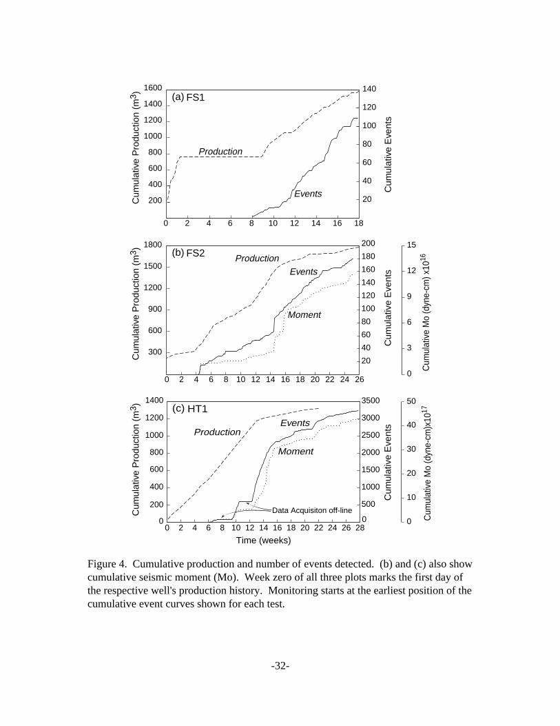
Gross production and event rates for the three monitor tests correlate, with changes in

rates lagging production rate changes by 2 to 3 weeks (Figure 4). The production curves sho

FS2 and HT1 include small contributions from other producing wells (<5% of total production

the respective study areas. Cumulative seismic moment for the FS2 and HT1 data sets are

shown (Figures 4b and 4c). We were able to obtain moment measurements for 78% of the e

comprising each of these data sets using low-frequency spectral amplitudes (Brune, 1970, eq

27). Moment-derived magnitudes (Hanks and Kanamori, 1979) range from -2.5 to 0.9 with

median of -1.0.

FS1 produced 762 m3 of oil by natural flow in the first 9 days following drilling (Figure 4a).

The well was then shut in for completion. Microseismic monitoring started week 8. Product

resumed week 9. The event rate increased during week 11, about 21/2 weeks after production

resumed. Event and production rates were fairly constant for the remainder of the FS1 test (F

4a).

Monitor Site(production

well)

Number ofEvents

Detected

Monitor Period(m/d/y)

TotalMonitorPeriod(weeks)

Downhole Geophone Stations(well: depth)

FS1 110 2/5/93 - 4/12/93 91/2 M: 335 m

FS2 180 9/17/93 - 2/8/94 201/2 M: 335 m M: 152 m

HT1 3237 1/8/95 - 8/5/95 30 GT8: 427 m GT8: 244 m BU1: 396 m

Table 1: Summary of events detected, monitor periods and geophone stations.

-5-

te

week

by a

ction

l

rate at

ion

hen

ginal

city

d put

r

g (L.

d the

to the

28,

HT1

han

es are

and the

ved at

ge

Monitoring of FS2 started 41/2 weeks after initial production (Figure 4b). The production ra

decline at week 6 has no corresponding decline in event rate. Pump rate was increased at

111/2 and is followed by an increase in event rate at week 141/2.Production decline at week 15 also

has no correlation to event rates, but the further decline in production at week 19 is followed

decrease in event rate at week 21 (Figure 4b).

The highest rates of seismicity and the strongest correlation of seismic activity with produ

were associated with the HT1 test (Figure 4c). Monitoring of HT1 began 6 weeks after initia

production. The decrease in production rate at week 13 is followed by a decrease in event

week 15. Production records for HT1 after week 22 are not available. We presume product

continued to decline from week 22 to 28. HT1 production was terminated during week 28 w

the well was deepened using an air-rotary rig. Deepening of HT1 directly connected the ori

productive interval with a water-filled (brine) fracture (located with production induced seismi

and discussed further below). HT1 was then plugged back to its original total depth (TD) an

back on-line. Production efforts were immediately terminated due to large volumes of wate

produced from the original production depth which had produced no water before deepenin

Wagoner, Ohio Kentucky Oil Corp., pers. commun., 1995). The presence of water indicate

previously produced interval was at least partially repressurized via the borehole connection

deeper fracture. A nearby lightning strike temporarily terminated monitoring beginning week

a few days before HT1 was deepened. Monitoring resumed from weeks ~301/2 to 36 during which

only 2 microearthquakes were detected (not shown in Figure 4c). In the 3 weeks before the

productive interval was inadvertently repressurized, the event rate was 120 times greater t

measured during the subsequent 51/2-week monitor period.

The correlation of the production and event rates suggests the observed microearthquak

triggered by production induced stress changes. The cumulative number of events detected

total seismic moment at the HT1 site were 18 and 37 times greater, respectively, than obser

site FS2, though comparable volumes were extracted from both locations (Figure 4). After

presenting an interpretation of the data, we will offer some speculation on the cause/effect

relationships, the 2 to 3 week lag time between production and seismicity rates and the lar

difference in cumulative seismic moment released at sites HT1 and FS2.

-6-

itor

s

three

).

were

first

and

ogs,

hole

ontal

make

tion

depth

ique

rence

the

ignal-

GT8.

with

their

re

ation

d

three

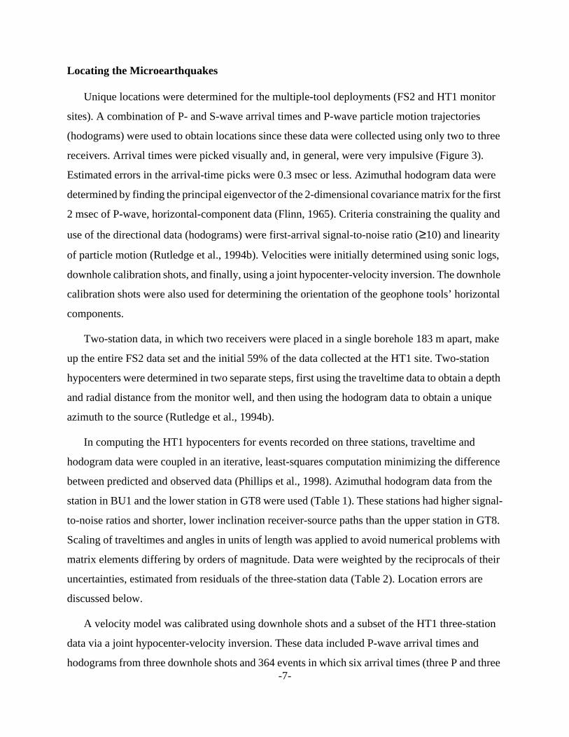
Locating the Microearthquakes

Unique locations were determined for the multiple-tool deployments (FS2 and HT1 mon

sites). A combination of P- and S-wave arrival times and P-wave particle motion trajectorie

(hodograms) were used to obtain locations since these data were collected using only two to

receivers. Arrival times were picked visually and, in general, were very impulsive (Figure 3

Estimated errors in the arrival-time picks were 0.3 msec or less. Azimuthal hodogram data

determined by finding the principal eigenvector of the 2-dimensional covariance matrix for the

2 msec of P-wave, horizontal-component data (Flinn, 1965). Criteria constraining the quality

use of the directional data (hodograms) were first-arrival signal-to-noise ratio (≥10) and linearity

of particle motion (Rutledge et al., 1994b). Velocities were initially determined using sonic l

downhole calibration shots, and finally, using a joint hypocenter-velocity inversion. The down

calibration shots were also used for determining the orientation of the geophone tools’ horiz

components.

Two-station data, in which two receivers were placed in a single borehole 183 m apart,

up the entire FS2 data set and the initial 59% of the data collected at the HT1 site. Two-sta

hypocenters were determined in two separate steps, first using the traveltime data to obtain a

and radial distance from the monitor well, and then using the hodogram data to obtain a un

azimuth to the source (Rutledge et al., 1994b).

In computing the HT1 hypocenters for events recorded on three stations, traveltime and

hodogram data were coupled in an iterative, least-squares computation minimizing the diffe

between predicted and observed data (Phillips et al., 1998). Azimuthal hodogram data from

station in BU1 and the lower station in GT8 were used (Table 1). These stations had higher s

to-noise ratios and shorter, lower inclination receiver-source paths than the upper station in

Scaling of traveltimes and angles in units of length was applied to avoid numerical problems

matrix elements differing by orders of magnitude. Data were weighted by the reciprocals of

uncertainties, estimated from residuals of the three-station data (Table 2). Location errors a

discussed below.

A velocity model was calibrated using downhole shots and a subset of the HT1 three-st

data via a joint hypocenter-velocity inversion. These data included P-wave arrival times an

hodograms from three downhole shots and 364 events in which six arrival times (three P and

-7-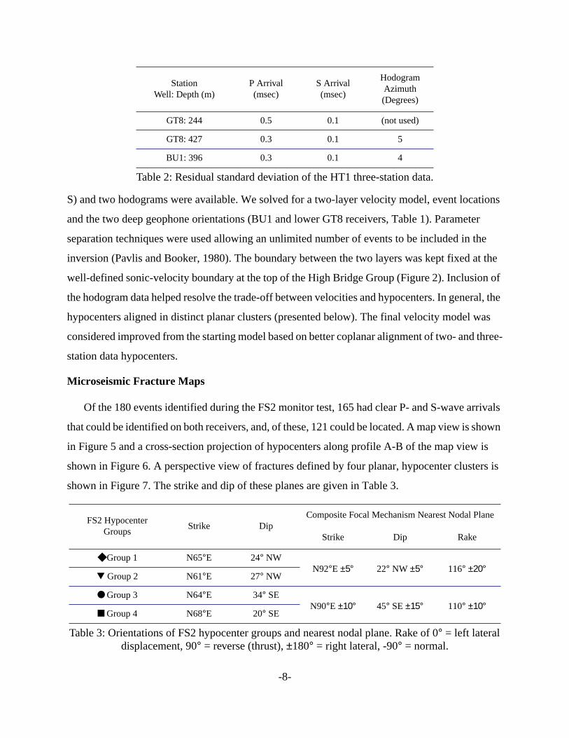

tions

ter

the

at the

of

ral, the

as

three-

rivals

hown

is

ers is

S) and two hodograms were available. We solved for a two-layer velocity model, event loca

and the two deep geophone orientations (BU1 and lower GT8 receivers, Table 1). Parame

separation techniques were used allowing an unlimited number of events to be included in

inversion (Pavlis and Booker, 1980). The boundary between the two layers was kept fixed

well-defined sonic-velocity boundary at the top of the High Bridge Group (Figure 2). Inclusion

the hodogram data helped resolve the trade-off between velocities and hypocenters. In gene

hypocenters aligned in distinct planar clusters (presented below). The final velocity model w

considered improved from the starting model based on better coplanar alignment of two- and

station data hypocenters.

Microseismic Fracture Maps

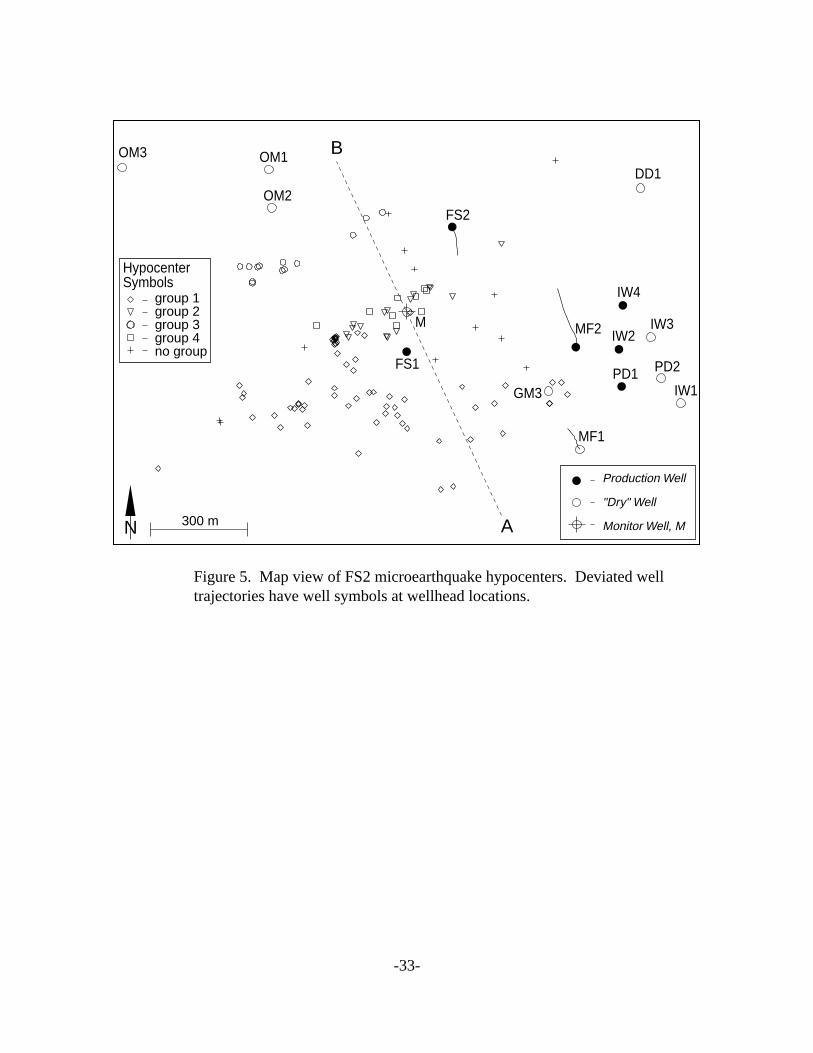
Of the 180 events identified during the FS2 monitor test, 165 had clear P- and S-wave ar

that could be identified on both receivers, and, of these, 121 could be located. A map view is s

in Figure 5 and a cross-section projection of hypocenters along profile A-B of the map view

shown in Figure 6. A perspective view of fractures defined by four planar, hypocenter clust

shown in Figure 7. The strike and dip of these planes are given in Table 3.

StationWell: Depth (m)

P Arrival(msec)

S Arrival(msec)

HodogramAzimuth(Degrees)

GT8: 244 0.5 0.1 (not used)

GT8: 427 0.3 0.1 5

BU1: 396 0.3 0.1 4

Table 2: Residual standard deviation of the HT1 three-station data.

FS2 HypocenterGroups

Strike DipComposite Focal Mechanism Nearest Nodal Plane

Strike Dip Rake

◆ Group 1 N65°E 24° NWN92°E ±5° 22° NW ±5° 116° ±20°

▼ Group 2 N61°E 27° NW

● Group 3 N64°E 34° SEN90°E ±10° 45° SE±15° 110° ±10°

■ Group 4 N68°E 20° SE

Table 3: Orientations of FS2 hypocenter groups and nearest nodal plane. Rake of 0° = left lateraldisplacement, 90° = reverse (thrust),±180° = right lateral, -90° = normal.

-8-

iew is

tion

e 8)

hown

S2

was

nal

m the

each

from

ut it

ue

igure

n

al.,

ique.

gh

these

ecting

tinct

For the HT1 microseismic data, 1719 of the 3237 events detected were located. A map v

shown in Figure 8. The majority of events (1548) are located east of well GT3. A cross-sec

projection of the events located east of GT3 along the profile line C-D of the map view (Figur

is shown in Figure 9. A perspective view of three fracture planes delineated east of GT3 is s

in Figure 10. Orientations of these planes are very similar to the fractures delineated near F

(Tables 3 and 4).

Except for the group C plane (Figure 10), grouping the hypocenters into planar clusters

accomplished by visual inspection using various 2-dimensional projections and 3-dimensio

graphic displays. The planar volumes shown in Figures 7 and 10 were then determined fro

eigenvectors of the covariance matrix of the 3-dimensional microearthquake locations within

group (Flinn, 1965). The strike and dip of the planes listed in Tables 3 and 4 were determined

the minimum eigenvectors (normals to the planes).

A hint of the group C events can be seen in the projection of Figure 9, dipping to the SE, b

is partially obscured by the events of larger group A. Group C was defined by a set of uniq

waveforms in which the S-waves observed on the upper geophone in GT8 were nodal (e.g. F

11). Comparison and grouping of waveforms, based on S to P amplitude ratios and locatio

constraints, has been used to identify planes within irregular volumes of seismicity (Roff et

1996). The identification of the group C plane (Figure 10) is a simple example of this techn

The waveforms observed on the upper geophone in GT8 are easily distinguished by the hi

amplitude P-wave and nearly nodal S-wave arrivals (e.g. Figure 11). Two hundred seven of

waveforms were identified and were found to define an elongate plane beneath, and inters

the northern edge of the larger, opposite-dipping, group A cluster (Figure 10). The very dis

seismicity boundary immediately south of GT8 is formed by this intersection (Figure 8)

HT1 HypocenterGroups

Strike DipComposite Focal Mechanism Nearest Nodal Plane

Strike Dip Rake

Group A N65°E 19° NW N47°E ±5° 27° NW ±5° 70° ±20°

Group B N82°E 17° SEN80°E ±35° 20° SE±10° 90° ±40°

Group C N67°E 16° SE

Table 4: Orientations of HT1 hypocenter groups and nearest nodal plane. Rake of 0° = left lateraldisplacement, 90° = reverse (thrust),±180° = right lateral, -90° = normal.

-9-

three-

f data

es in

rror

tance

olely

n 250

rrors

ts that

to 20

the

the

lls.

the

fit fault

single

ontal

hone

n of

(

are

lanes

-SE at

T

and 4)

Location errors

Uncertainties for both the FS2 and HT1 data were estimated from residuals of the HT1,

station data (Table 2). These errors only reflect the station-event geometry, the distribution o

types, and data uncertainties; velocity model uncertainties were not considered. Error ellips

general are linear and trend perpendicular to the event-station direction due to the larger e

contribution associated with the hodogram azimuths (Table 2). Error in depth and radial dis

from the monitor boreholes are predominantly associated with the arrival time uncertainties (s

for the two-station locations) and, hence, are smaller. For the two-station event location the

maximum axis of the error ellipsoids are horizontal and ranged between 10 and 20 m withi

m of the monitor boreholes, and up to 75 m for the most distant events (850 m).The location e

for the HT1 three-station data east of GT3 (Figures 8 and 9) range between 3 and 5 m. Even

lie close to the N-S plane through the two monitor boreholes (GT8 and BU1) have errors up

m and ellipses that are highly linear, trending E-W. Well-log porosity anomalies corroborate

intersection of the seismically-active fractures at wellbores (presented below). Accuracy of

intersection of the group-computed planes, defined by the maximum and intermediate

eigenvectors, with the log anomalies ranges from 0.5 to 3 m within 250 m of the monitor we

Fault Plane Solutions and State of Stress

Composite fault plane solutions were computed for the planar hypocenter groups using

computer program FPFIT (Reasenberg and Oppenheimer, 1985). Figure 12 shows the best

plane solutions for the FS2 and HT1 groups identified in Figures 7 and 10. Convergence to a

solution was achieved in each case. First motion data from all receiver tools were used. Horiz

component first motions were used, after correcting for tool orientation, from the deeper geop

tools with lower inclination source-receiver paths. Hypocenter planes with the same directio

dip were combined to improve the focal sphere coverage. Discrepant first motions were few≤9%) except for the HT1 group A plane (22%). However, most of the HT1 group A discrepants

associated with the GT8 upper-geophone-tool first motions which straddle one of the nodal p

where uncertainty in polarity would be greatest (Figure 12c). All four composite fault plane

solutions indicate a predominantly thrust mechanism. P axes are consistently oriented NW

near-horizontal inclination. Uncertainty within the 90% confidence limit are shown for P and

axes (Figure 12) and listed for the nodal plane closest to the mapped fault planes (Tables 3

-10-

f a

d 4).

ted

r

r-

ar

e, the

litudes

roup

e

ngle

lic

, 1996).

990)

of

nt of

h the

ding

at 5

in

rved

ce

(Reasenberg and Oppenheimer, 1985).

The four composite focal mechanisms are consistent and show fairly good agreement o

nodal plane orientation with the hypocenter-determined planes (Figure 12 and Tables 3 an

This suggests that the assumption of common mechanisms occurring along similarly-orien

rupture surfaces within the mapped planes is good. The median area of rupture surfaces fo

individual events is only about 50 m2 (Schuessler et al., 1995), whereas the larger hypocente

defined planes have areas up to 3.5 x 105 m2. S-P amplitude ratios are also consistent with coplan

orientation of the individual rupture surfaces and the larger, mapped planes. As an exampl

first motions for the group C plane recorded on the GT8 upper receiver are centered in the

compressive quadrant of Figure 12d, where, as observed (Figure 11), the P- and S-wave amp

should be anti-nodal and nodal, respectively (Aki and Richards, 1980, p. 82). The dip of the g

C plane is within 8° of the theoretical orientation at which this amplitude relationship would b

observed at the GT8 upper receiver for pure reverse-slip motion at the plane centroid. Our

observations indicate uniform sense of motion, preferentially along similarly-oriented, low-a

faults. This is in contrast to highly variable focal mechanisms observed during large hydrau

fracture operations (e.g. House and Jensen, 1987; Cornet and Jianmin, 1995; House et al.

Presumably this uniform seismic slip is controlled by the background state of stress.

Stress

Principle stress orientations and relative magnitudes were computed using Gephart’s (1

focal mechanism stress inversion computer program (FMSI) which implements the method

Gephart and Forsyth (1984). The four composite focal mechanisms are the minimum amou

data required to implement this procedure. Input data were the nodal plane orientations wit

fault planes identified, in all four cases, as the nodal plane closest to the mapped planes.

Knowledge of the correct fault planes helped constrain the solutions. The exact method of fin

the best stress model was conducted using a grid search over the entire lower hemisphere°

increments (Gephart and Forsyth, 1984). Resultant principle stress orientations are shown

Figure 13 within the 95% confidence limit. Average angular rotation required to bring the obse

fault planes and slip direction into agreement with the final model (within the 95% confiden

limit) is <5°. Maximum principle stress, , is near horizontal, trending N15°W ±15°. The smallσ1

-11-

and

itude

e

icated

near-

rom

regime

o the

More

red

alous

ess

ealed

se

story.

as

number of focal mechanisms and the similar orientations of active faults observed leave the

orientations more poorly resolved (Figure 13). Correspondingly, the relative stress magn

R (where ) was poorly resolved, ranging from 0.65 to 0.95 within th

95% confidence limit.

Relatively high compressive stress at the shallow depths (<550 m) of the study area is ind

by the thrust type fault-plane solutions and the stress inversion. Evans (1989) has shown a

surface (<600 m) thrust stress regime to be ubiquitous throughout the Appalachian Basin f

eastern Kentucky to western New York. Our data indicate that this same near-surface stress

persists further south and west. Orientation of maximum horizontal stress (SH) at our shallow depth

of measurements (SH= ) is rotated approximately 90° from the regional direction. SH is

consistently oriented ENE-WSW from the U.S. midcontinent region, west of our study area, t

eastern side of the Appalachians (Zoback and Zoback, 1980; Evans, 1989; Zoback, 1992).

specifically, in central Kentucky SH direction would be expected to be between values measu

in eastern (N51°E) and western (N81°W) Kentucky (Plumb and Cox, 1987). The rotation of SH

from expected regional orientation may be due to local structural control. Further, this anom

stress orientation may only exist at shallow depth due to variation in principle horizontal str

gradients at the near surface, resulting in SH and Sh being flipped with respect to orientation at

greater depth (Sh=minimum horizontal stress).

Interpretation

At both production sites along the Indian Creek syncline, the microearthquakes have rev

sets of low-angle thrust faults within and immediately above the High Bridge formation. The

thrust faults strike about N65°E and dip to both the NW and SE at angles ranging from

approximately 15° to 35° (Tables 3 and 4). Below, we summarize the relationship of the

seismically-active fractures with respect to production, local geology and inferred pressure hi

Seismically-Active Fractures and Production

The seismically-active fractures occur away from or outside of currently-drained depth

intervals. While monitoring FS2, 95% of the fluid volume extracted in the immediate area w

σ2

σ3

R σ2 σ1–( ) σ3 σ1–( )⁄=

σ1

-12-

r

r

, the

p and

up 1)

ly to

ave

rs

M is

was

ter

tary

t it is

M in

ave

67 m

sity-

pth.)

ould

ent to

p 1

produced from FS2 (about 1750 m3). Well FS1 was intermittently on-line during the FS2 monito

period and contributed about 2% (40 m3) of the oil production plus some small volume of wate

(water volume records were not kept). The other 3% (48 m3) came from well PD1 during the last

5 weeks of monitoring (Figures 5, 6 and 7). Along the strike direction of the mapped planes

production-depth interval of FS2 projects close to the two minor fractures delineated by

hypocenters groups 2 and 4 (Figure 6), but is located east of these fractures as seen in ma

perspective views (Figures 5 and 7, respectively). The largest seismically-active fracture (gro

is clearly outside of the production depth intervals of FS2 and FS1 (Figures 6 and 7).

A similar relationship was observed during monitoring of HT1; 97% of the fluid volume

extracted during monitoring was produced from HT1 (> 1300 m3). The seismicity occurs both

above and below the production interval of HT1 (Figures 9 and 10) and, in map view, primari

the west of HT1 (Figure 8).

The seismically-active fractures have been partially drained by previous production and h

subsequently been resaturated with brine (water).Three of the fractures mapped on the Summe

lease are intersected by the monitor well M (hypocenter groups 1, 2 and 4 of Figure 7). Well

an old production well drilled in the late 1940’s, identified as the Summers #3 well in Wood

(1948), and is currently water-filled, uncased and obstructed at 378 m. The original TD of M

489 m which puts the well termination at the base of the major fracture defined by hypocen

group 1 (Figures 6 and 7). When drilled, cable-tool drilling was used in the area. Like air-ro

drilling, cable-tool drilling is typically terminated when substantial fluid flow is encountered.

There are no records of the depth intervals produced or volumes extracted from well M, bu

likely that the group 1 fracture intersected at the original TD was at least partially drained by

the late 1940’s. Whether group 2 and 4 fractures were originally water or oil filled, they would h

undergone some drainage during drilling. The intersection of the group 2 fracture at about 2

depth is corroborated with a density-derived porosity anomaly from 267 to 269 m. (The den

log interval was terminated above the group 4 fracture intersecting well M at about 366 m de

Since well M is open to formation and water filled, the three fractures intersecting the well sh

be at hydrostatic pressure. The group 1 plane was intersected by well GM3, drilled subsequ

monitoring, in April, 1995. Brine was encountered at 313 m where GM3 intersects the grou

plane (Figures 5, 6 and 7).

-13-

T2,

with

p-dip

r

hen

rature-

y

f 725

-line

not

).

er

drill

with

ek

group

brine.

ay

ure 14

ion

n

sts

t on

with

ame

At the HT1 site the seismically-active fractures and production history show a similar

relationship. In map view the main seismic zone is bounded by older production wells, GT1, G

GT3 and GT4 (Figure 8). Production depth intervals of GT1, GT2 and GT4 intersect or align

the seismically-active fractures (Figures 9 and 10). GT4’s production interval intersects the u

side of the A fracture. GT2’s upper production interval intersects the B fracture and its lowe

production interval, brought on-line after deepening the well, aligns with the C fracture. The

productive interval of GT1 aligns with the A fracture’s down-dip side (Figures 9 and 10). W

deepened, GT2 also intersected the up-dip side of the A fracture and is correlated with tempe

and neutron-porosity log anomalies. GT2 did not produce oil from the A fracture, most likel

because of partial drainage already underway from GT1 and GT4. A cumulative oil volume o

m3 was extracted from these 3 wells in the 9 months proceeding monitoring. Only GT1 was on

with HT1 during monitoring, and it only contributed an additional 25 m3 of oil. Small volumes of

water (brine) were also produced from GT1, GT2 and GT4 (water production records were

kept). HT1 produced no water (L. Wagoner, Ohio Kentucky Oil Corp., pers. commun., 1995

A test well, GT10, was drilled by the Ohio Kentucky Oil Corporation (OKOC) into the low

edge of the group A fracture after 5 months of monitoring. No fluid was encountered until the

bit reached the group A fracture at 432 m (Figures 8, 9 and 10). The fracture produced brine

drill-string air circulation (air rotary drilling) and drilling was immediately terminated. One we

later, OKOC deepened HT1 and also encountered brine when the well intersected the same

A fracture further up dip at 404 m (Figures 9 and 10). Below, we discuss the source of the

Production wells PD1, IW2, IW4 and MF2 (Figures 5, 6, and 7) are located about halfw

between the FS2 and HT1 monitor sites. These four wells are also shown unmarked in Fig

in between the FS2 and HT1 hypocenters. A cumulative 719 m3 of oil was extracted from PD1,

IW2 and IW4. MF2 was a potential producer but was never put on-line due to well complet

problems. Ninety-one percent of the oil (654 m3) was produced during the 11-month gap betwee

the FS2 and HT1 geophone deployments (Table 1). Production from PD1 spanned both te

contributing only 48 m3 during FS2 monitoring and 17 m3 during HT1 monitoring. Along the

strike direction of the active fractures, production-depth intervals of PD1, IW2 and IW4 projec

or close to the group 1 fracture (Figures 6 and 7). The HT1 group A cluster aligns at depth

group 1 when plotted with respect to the same elevation and is probably extension of the s

-14-

is

set

ecting

or

the

l of

tured,

here

um

82, p.

r

nly be

can

y the

The

ll-log

a

is

tion of

ar

esume

lly-

ature

structure. The extent of east-west permeability continuity along the group 1 - group A fault

unknown.

Along the Indian Creek syncline, the oil reservoir in the High Bridge Group is primarily a

of comparted, low-angle thrust faults. This conclusion follows from the correlation of the older

production depth intervals and the mapped, low-angle thrust faults. Logged boreholes inters

the seismically-active fractures show distinct porosity-log anomalies (density, neutron and/

temperature) over 1 to 2 m intervals. Density-neutron porosity logs are shown in Figure 15 for

seismically-active productive interval of GT1 and the seismically-inactive productive interva

HT1. These are examples in which the boreholes were not enlarged or irregular over the frac

productive zones, allowing reliable log-porosity estimates to be obtained. Over the intervals w

the density-derived porosity exceeds the neutron porosity (the gas-crossover effect), maxim

porosity is estimated as the root-mean-square (rms) of the two peak log values (Asquith, 19

68). Using the log values averaged over 1 m of thehighest porosity intervals exhibiting crossove

as inputs to the rms computation, gives a 7% average porosity for both the GT1 and HT1

productive zones. The 1 m thickness associated with the average porosity estimates can o

considered a maximum thickness of the porous, fracture intervals since the displayed logs

represents data smoothed or averaged over larger depth intervals. From these values, we

roughly estimate an upper limit of a mapped fracture’s pore volume.

For the group A fracture we estimated pore volume using the surface area delineated b

microseismicity and fracture-zone thickness and porosity estimated from the GT1 log data.

active area of the fracture mapped east of GT3 is approximately 300 by 100 m. Using the we

estimate of 7% porosity developed over a 1 m interval gives a total pore volume of 2100 m3.

Productive intervals of GT1 and GT4, which align with the group A fracture zone, produced

cumulative 402 m3 of oil or 19% of the fracture’s computed pore volume.

The correlation of the event rates and HT1 production suggests that the microseismicity

triggered by the current-production induced stress changes (Figure 4c). The spatial correla

the microseismicity to past production in turn suggests that current drainage follows a simil

pattern. Based on these inferences and the similarity of the log responses (Figure 15), we pr

that HT1 also produces from a low-angle fracture oriented similar to the adjacent, seismica

active fractures. A plane formed by the productive intervals of HT1, GT3 and a weak temper

-15-

HT1

illed

ith

maly

(the

log

GT2

tivity

, are

strike

in the

fracture

bout

in

also

ip

face

ain in

y

Creek

995).

ting

anomaly in GT10, at 354 m, strikes N72°E and dips 22° SE, consistent with the mapped thrust-

faults (Tables 3 and 4 and Figure 10). GT3 was the second, single largest producer in the

monitor area (544 m3) and also produced at a depth interval between the seismically-active

fractures. The inferred fracture would have been partially drained by GT3 before HT1 was dr

and intersected it further down dip (Figure 10). Initial production response supports this

interpretation. GT3 initially flowed oil to surface, HT1 did not. Test well GT10 aligns closest w

HT1 and GT3 along strike of the microseismic mapped structures, and its temperature ano

gives the third point defining the plane. The GT10 log showed no other significant anomalies

group A fracture intersected at TD could not be spanned by the logging tool). There are no

anomalies indicating the inferred fracture intersects the surrounding production wells GT1,

and GT4. Production history also indicates these wells have very poor or no hydraulic conduc

with the volume drained by HT1. Permeability and porosity of the inferred fracture, therefore

developed over a narrow zone in the dip direction (<60 m at S18°E). The narrow zone of seismicity

extends about 850 m SW of HT1 (Figure 8) suggesting an extensive pressure response in the

direction. Evidence of immediate pressure communication between wells has been observed

area at distances greater than 1 km and has been interpreted as intersection with a common

(J.H. Perkins, Petro-Hunt, Inc., pers. commun., 1996).

Local Geologic Structure

Historical displacements along the imaged thrust faults are small with vertical throws of a

1 m or less (Hamilton-Smith, 1995). Detailed log correlations show about 1 m of thickening

section just above the group 2 mapped thrust fault (Figure 7). The observed thickening could

be due to local infill sedimentation. We can conclude that total historical displacements in d

direction do not exceed about 2 m.

The east-west trending Indian Creek syncline is a very low-relief structure mapped

predominantly from Mississippian outcrops (Lewis and Thaden, 1962, 1965). Local subsur

expression of the structure at the top of the High Bridge Group is shown in Figure 1 and ag

Figure 14 with the FS2 and HT1 microearthquake locations. The surface structure is clearl

associated with a basement graben seen on a reflection seismic profile crossing the Indian

syncline near wells FS1 and FS2 (S.K. Jones, Meridian Exploration Corp., pers. commun., 1

The structural low propagates upward with diminished relief and depositional infilling sugges

-16-

ent-

ling

acture/

with

lying

nly

h en

ing,

e

y

ure

rvoir

es.

ells

gh-

n

sured

ld

(oil

l

episodic, Paleozoic reactivation of the basement structure (Hamilton-Smith, 1995). Basem

controlled wrench faults have been associated with synclinal oil production from shallow,

fractured, Ordovician carbonates 65 km west of Clinton County (Black, 1986a). Recent dril

programs along the Indian Creek syncline have been based on a similar interpretation of fr

lineament patterns delineated on side-looking airborne radar images. Features associated

these structures are secondary faults and fold axes lying en echelon along the main, under

fault, formed by strike-slip displacement of the deeper fault (Harding, 1974). In Kentucky, o

near vertical fracture sets have been considered in the wrench-fault interpretations, althoug

echelon thrust faults should also be expected with convergent, strike-slip movement (Hard

1974). The significant result of the microseismic monitoring has been the identification of th

small-displacement thrust faults and their association with oil production. Though previousl

unidentified, these structures, lying along and striking oblique (~N65°E) to the east-west trending

Indian Creek syncline (Figure 14), are consistent with Hamilton-Smith’s (1995) and local

operators’ right-lateral, wrench-fault interpretations.

Pressure History

In this section we attempt to describe the reservoir pressure history and estimate press

changes that may be inducing the observed microseismicity. In the absence of known rese

pressure measurements, we base this description on some simple assumptions and field

observations that at least allow us to arrive at reasonable limits of reservoir pressure chang

Initial production in the study area is characterized by high-volume flow to the surface. W

are typically put on pump within a few days of discovery as pressure declines. Based on hi

volume flow to surface, it has been suggested that the reservoirs are initially overpressured

(Hamilton-Smith, et al., 1990; Hamilton-Smith, 1995). Hydrostatic head alone, however, ca

account for the observed flow. Well FS1, for example, flowed 236 m3 to a tank battery elevated

about 12 meters above the wellhead within the first 24 hours of production. Water levels mea

in static wells open to reservoir depth correspond to 3 m below the FS1 wellhead. This cou

support a column of oil in FS1 from the production depth at 305 m to 63 m above the wellhead

density = 0.82 g/cm3 (Hamilton-Smith, 1995)). Brine in the geologic section and gas in the oi

would increase the oil’s buoyancy.

-17-

icated

and

tion).

along

slip.

servoir

th far-

ssure

as a

r, the

ths

y the

rom

and

sion

,

rom

p

al

e

The drained fractures eventually recover to hydrostatic pressure via brine invasion as ind

by fluid levels in wells intersecting the seismically-active fractures. Water levels in well M

(Figures 6 and 7) were repeatedly measured at 13 m depth (247 m elevation) throughout

monitoring. Well GT2 connects with the seismically-active fractures at the HT1 site (Figures 9

10) and was also water-filled to the near surface during monitoring (37 m depth, 249 m eleva

If the reservoir is initially overpressured it implies that a net pore-pressure decrease occurs

fractures from pre-drainage to subsequent hydrostatic recovery, which would inhibit seismic

Therefore, the observed seismic failure along the pressure-cycled fractures suggests the re

cannot be overpressured. We assume instead that the reservoirs are initially in equilibrium wi

field pore pressure (hydrostatic) so that little or no net pressure change results from the pre

cycling. In fact, a small pressure increase should occur along the pressure-cycled fractures

result of produced oil being replaced with denser brine (discussed further below).

The evidence of brine invasion along the previously productive fractures with eventual

hydrostatic pressure recovery suggests a natural water drive is active in the area. Howeve

water drive is very poorly connected to the productive fractures via natural reservoir flow pa

and is unable to maintain reservoir pressure during drainage. Pressure decline is evident b

short duration of flow to the surface. Hydraulic isolation of the productive fractures is evident f

very low to nonexistent water (brine) production during the wells’ short productive histories

the highly comparted nature of production from adjacent, sequentially drilled wells. Brine inva

and pressure recovery of the drained fractures is often facilitated by open-well completions

allowing direct communication between permeable zones at different depths.

An upper limit of reservoir pressure decline would be due to complete removal of fluid f

the production well by pumping. This limit is reasonable because as pressure declines, pum

capacity can surpass inflow to the wells. Pumping is then cycled allowing intermittent, parti

fluid-level recovery in the well. Assuming the reservoir was initially at hydrostatic pressure,

emptying the well is equivalent to a pressure drop (∆p) by removal of about 300 m of brine. Using

an assumed density of sea water (ρ=1.03 gm/cm3) ∆p = -3 MPa. Pressure reduction away from th

borehole would be less.

-18-

rved

s due

ive

e

tress

nd

e. At

ions

e of

994).

d a

Pa.

h

hereby

ment

on

,

Production-Induced Stress Change

We consider two possible mechanisms by which production may be promoting the obse

seismic slip: 1) increased horizontal compression above and below currently drained volume

to poroelastic effects, and 2) reduction of effective normal stress across previously product

fractures due to brine replacing oil.

Poroelastic stresses will be generated outside a drained volume due to contraction of th

reservoir rock accompanying production (e.g. Segall, 1989). The magnitude of horizontal s

change∆σh centered just above or below an axisymmetric, flat-lying ellipsoidal volume

undergoing uniform pressure change∆p is given by whereα is the Biot

coefficient,υ is Poisson’s ratio and a1 and a3 are the reservoir semi-major axes in horizontal a

vertical directions, respectively (Segall and Fitzgerald, 1998). Compressive stress is positiv

the HT1 site a3/a1 = 0.5 m/30 m = 0.017 corresponding to the inferred, drained fracture dimens

in theσ3-σ1 plane (a3 from HT1 well log, Figure 15, and a1 from the length along dip direction,

Figure 10).α = 0.43 was determined using a log-derived porosity of 7% and an empirical curv

α versus porosity for carbonate rocks (Laurent et al., 1990) as summarized by Segall et al. (1

υ = 0.36 was determined from the seismic velocities (Figure 2). Using these parameters an

pressure drop <3 MPa,∆σh outside the currently-drained volume at the HT1 site is <0.008 M

Pressure re-equilibration of the previously productive fractures by replacement of oil wit

denser brine will result in a small pore pressure increase relative to pre-drained pressure, t

decreasing effective normal stress across the fracture. Uniform drainage and brine replace

along the fractures will result in a pressure increase∆p =∆V∆ρgh where∆V is the portion of pore

volume produced as oil,∆ρ is the density difference of brine and oil, g is gravitational accelerati

and h is the height of the fracture due to its dip. For the group A fracture, (Figures 9 and 10)∆V

= 19% (presented above),∆ρ = (1.03 - 0.82) = 0.21 gm/cm3, and h = 35 m maximum, giving a

maximum∆p = 0.014 MPa along the deepest portion of the seismically-active fracture.

∆σh α– ∆p1 2υ–1 υ–

--------------- π

4---

a3

a1-----=

-19-

hips

s the

nce of

-

l, slip

n

across

.

d by

lastic

ges are

rence

of pore

ering

ns of

tic

all as 0.01

lastic

f tidal-

one to

pends

ble

ated,

panying

ociated

ear

of

.

stress,

Discussion

Both triggering mechanisms seem plausible in light of the spatial and temporal relations

observed between production and seismicity. The temporal correlations (Figure 4) suggest

seismicity is triggered by current-production induced stress changes, and the spatial occurre

the seismicity is similar to that expected for Segall’s (1989) poroelastic model of extraction

induced stress changes for relatively flat-lying drainage volumes. Consistent with the mode

is inhibited along the currently-drained fracture (e.g. the inferred, aseismic fracture shown i

Figure 10) because the effective stress loading predominantly increases the normal stress

the fracture; reverse slip is triggered on fractures above and below the drained volume (e.g

fractures A, B and C of Figure 10) due to small increases in horizontal compression induce

production. As is our case, reverse faulting triggered above or below the reservoir by poroe

compression would only be expected within a thrust stress regime because the stress chan

so small (Segall, 1992; Segall et al., 1994; Segall and Fitzgerald, 1998). In addition, the occur

of seismicity along the surrounding, pre-drained fractures also suggests that the mechanism

pressure increase, or reducing effective normal stress via brine invasion, may itself be trigg

shear slip or at least driving the pressure-cycled fractures closer to shear failure.

Magnitude of total estimated stress change promoting slip is about 0.02 MPa. Correlatio

increased aftershock activity occurring in regions where computed, mainshock-induced sta

stress has also increased, suggests earthquakes can be triggered by stress changes as sm

to 0.05 MPa (Reasenberg and Simpson, 1992; Stein et al., 1992). Our estimated limit of poroe

stress change outside currently-drained volumes (<0.008 MPa) is approaching magnitudes o

induced stress change (0.005 MPa, Stacey, 1969, p. 217) and may not be great enough al

trigger slip. The relative importance of the poroelastic and oil-replacement stress changes de

on the log porosity estimates, though total stress change will not vary much within reasona

limits of porosity. If, for example, the logs used are not representative of the overall fracture

porosity away from the boreholes, and fracture pore volume is actually larger than we estim

then the poroelastic-induced compression increases and the pore-pressure change accom

oil replacement becomes smaller. As in the studies cited above, the small stress changes ass

with seismicity implies that the active fractures or faults are already critically stressed for sh

failure within the background state of stress, and, in our case, further implies a correlation

critically stressed reservoir fractures with production (porosity and permeability anomalies)

Seismicity triggered by small stress changes, in turn, should reflect the background state of

-20-

ve

d HT1

during

). Wells

(group

ically-

ional

ion or

n well

if the

d event

the

ssure

but the

ssure

n. The

ved

fter

more

mall-

vals

. The

ations

exhibiting uniform focal mechanism on similarly oriented faults, consistent with what we ha

observed (Figure 12).

The discrepancy in number of events and total seismic moment observed at the FS2 an

sites (Figure 4) may be due to the older production history near the FS2 site. Events rates

the FS1 test were comparable to the subsequent and adjacent FS2 test (Table 1 and Figure 4

FS1 and FS2 are located on the margins of the older Seventy-Six oil field, developed and

abandoned in the late 1940s (Figure 14). The most seismically-active fracture at the FS2 site

1, Figure 7) was probably productive 45 to 50 years ago, whereas, at the HT1 site, the seism

active fractures were produced in the 7 months before HT1 came on-line. Release of addit

strain energy at the FS1-FS2 production site could have occurred during the earlier product

more gradually over the intervening 45 to 50 years before production activity resumed.

Finally, we computed pressure response versus time at 150 m distance from a productio

using Theis’s (1935) solution for a confined aquifer (Freeze and Cherry, 1979, p. 317) to see

response provided any insights to the 2 to 3 week delays observed between production an

rates. One-hundred-fifty meters corresponds to the horizontal distance from the HT1 well to

center of the most seismically-active fracture (group A, Figures 8, 9 and 10). Computed pre

decline and recovery magnitudes varied for a range of reasonable hydrogeologic properties,

delay characteristics were similar in all cases. As shown in the example of Figure 16, the pre

response at 150 m is strongly affected almost immediately by step-rate changes in productio

response curves for pressure within the currently-drained fracture do not explain the obser

delays unless some pressure thresholds controlling failure rate are crossed 2 to 3 weeks a

production-rate changes. Determining what the pressure thresholds might be would require

accurate knowledge of the reservoir’s hydrogeologic properties.

Conclusions

Mapping the production-induced microseismicity has revealed previously undetected, s

displacement, low-angle thrust faults. Correlation of these faults with older production inter

and well-log porosity anomalies indicates that these types of features should be considered

potentially important drilling targets in the continued exploration and development of the area

microseismicity only reveals those fractures or faults with a propensity to slip due to their

orientation with respect to the current state of stress. Barton et al. (1995) have shown correl

-21-

less

ations.

n (e.g.

may

onal

gh

s

higher

lts are

lower

ng,

offer

r

ovide

tures

ature

ce the

Steve

ht,

udy.

y

for

uy

land.

of much higher permeability along fractures oriented optimally for shear failure than fractures

critically stressed in current stress fields. Our study appears to further support those correl

Surface lineament and outcrop studies indicate a complex variety of fracture sets in the regio

Black, 1986b; Hamilton-Smith, 1995). Other fracture sets or faults present in the study area

play an important role in compartmentalizing the productive, low-angle faults.

The small-displacement thrust faults pose a difficult exploration problem using conventi

seismic reflection data; they are too thin (<2 m) to be imaged directly and do not have enou

vertical throw to resolve bedding discontinuities. Consideration of the low-angle fractures a

exploration targets will probably require inference from other features such as the deeper,

relief basement structures seen on reflection seismic data in the area. If the shallow thrust fau

indeed associated with a basement-controlled wrench structure, then they may be part of f

structures, steepening and converging with the main fault zone at greater depth (see Hardi

1990).

The identification of the productive, low-angle fractures also has implications for field

development. Drilling horizontal or deviated wells at these shallow depths does not appear to

any advantage in increasing the probability of intersecting productive fractures. Dip meter o

formation microscanning logs would be useful in determining orientations of low-angle,

productive fractures, enabling interwell correlation and mapping of pay zones, and further, pr

guidance in offset well placement. Interwell correlation and mapping of the conductive frac

will also allow improved planning in plug-and-abandonment operations so as to avoid prem

water invasion of pay zones. Pressure maintenance operations could also be attempted on

conductive fracture zones between wells have been mapped.

Acknowledgment

We thank Dave Anderson, Tom Fairbanks, Grady Rhodes, Rick Flora, Joel Duran and

Harthun for their many hours contributed to field work. We gratefully acknowledge Jim Albrig

Jay Bertram, Jim Drahovzal and Bob Hanold for their efforts in initiating and supporting this st

Don Dreesen, Terry Hamilton-Smith, Hunt Perkins, Steve Jones, Lynn Wagoner and Harve

Young provided valuable discussions on data interpretation. Thanks to Wayne Pennington

providing helpful guidance in determining log-porosity estimates. We are also grateful to G

Tallent and the late Frank Summers for allowing us to place monitoring equipment on their

-22-

ogy

dian

ory

es,

tion:

.H.

,

by

o. Eng.

r.

ent

n

. J.

This work was supported by the U.S. Department of Energy’s Natural Gas and Oil Technol

Partnership. Participants included the Ohio Kentucky Oil Corporation, Petro-Hunt, Inc., Meri

Exploration Corp., Ramco Energy Corporation, Petro-7, Inc., Los Alamos National Laborat

and the Kentucky Geological Survey. Sonic-log data was provided by Touchwood Resourc

Michael P. Hanratty, Polaris Energy and Trey Exploration, Inc.

References

Albright, J.N. and Pearson, C.F., 1982. Acoustic emissions as a tool for hydraulic fracture loca

experience at the Fenton Hill hot dry rock site. Soc. of Petro. Eng. J., 523-530.

Aki, K. and Richards, P.G., 1980. Quantitative seismology, theory and methods, volume 1. W

Freeman and Co., San Francisco.

Asquith, G. 1982, Basic well log analysis for geologist. Am. Assoc. Petro. Geologists, Tulsa

Oklahoma.

Barton, C.A., Zoback, M.D. and Moos, D., 1995. Fluid flow along potentially active faults in

crystalline rock. Geology, 23, 683-686.

Batchelor, A.S., Baria, R. and Hearn, K., 1983. Monitoring the effects of hydraulic stimulation

microseismic event location, a case study. SPE paper 12109, presented at 58th Soc. Petr

Annual Technical Conference and Exhibition, San Francisco, California.

Black, D.F.B., 1986a. Oil in dolomitized limestone reservoirs in Kentucky. In: M.J. Aldrich, J

and A.W. Laughlin (Editors), Proceedings of the 6th International Conference on Basem

Tectonics. Int. Basement Tectonics Assoc., Inc., Salt Lake City, Utah.

Black, D.F.B., 1986b. Basement faulting in Kentucky. In: M.J. Aldrich, Jr. and A.W. Laughli

(Editors), Proceedings of the 6th International Conference on Basement Tectonics. Int.

Basement Tectonics Assoc., Inc., Salt Lake City, Utah.

Block, L.V., Cheng, C.H., Fehler, M.C. and Phillips, W.S., 1994. Seismic imaging using

microearthquakes induced by hydraulic fracturing. Geophysics, 59, 102-112.

Brune, J., 1970. Tectonic stress and the spectra of seismic shear waves from earthquakes

Geophys. Res., 75, 4997-5009.

-23-

ation

d of

are

-986.

elation

roc.

ew

ake

stress

uake

Cornet, F.H. and Jianmin, Y., 1995. Analysis of induced seismicity for stress field determin

and pore pressure mapping. Pure Appl. Geophys., 145, 677-700.

Davis, S.D. and Pennington, W.D., 1989. Induced seismic deformation in the Cogdell oil fiel

west Texas. Bull. Seism. Soc. Am., 79, 1477-1494.

Deflandre, J.P., Laurent, J., Michon, D. and Blondin, E., 1995. Microseismic surveying and

repeated VSPs for monitoring an underground gas storage reservoir using permanent

geophones. First Break, 13, 129-138.

Doser, D.I., Baker, M.R. and Mason, D.B., 1991. Seismicity in the War-Wink gas field, Delaw

Basin, Texas, and its relationship to petroleum production. Bull. Seism. Soc. Am., 81, 971

Eberhart-Phillips, D. and Oppenheimer, D.H., 1984. Induced seismicity in The Geysers

geothermal area, California. J. Geophys. Res., 89, 1191-1207.

Evans, K.F., 1989. Appalachian stress study 3. Regional scale stress variations and their r

to structure and contemporary tectonics. J. Geophys. Res., 94, 17619-17645.

Fehler, M., House L. and Kaieda, H., 1986. Seismic monitoring of hydraulic fracturing:

Techniques for determining fluid flow paths and state of stress away from a wellbore. In: P

27th U.S. Symposium on Rock Mechanics. Tuscaloosa, Alabama, June 23-25.

Flinn, E.A., 1965. Signal analysis using rectilinearity and direction of particle motion. Proc.

I.E.E.E., 53, 1725-1743.

Freeze, R.A. and Cherry, J.A., 1979. Groundwater. Prentice-Hall, Inc., Englewood Cliffs, N

Jersey.

Gephart, J.W., 1990. FMSI: A FORTRAN program for inverting fault/slickenslide and earthqu

focal mechanism data to obtain regional stress tensor. Comput. Geosci., 16, 953-989.

Gephart, J.W. and Forsyth, D.W., 1984. An improved method for determining the regional

tensor using earthquake focal mechanism data: application to the San Fernando earthq

sequence. J. Geophys. Res., 89, 9305-9320.

-24-

rvoir

eek

etro.

. Pure

ll.

y:

h-

11,

348-

logist

a and

ulic

on in

Gooding, P.J., Kuhnhenn, G.L. and Kiefer, J.D., 1988. Depositional environments and rese

characteristics of the Lower Ordovician Knox Group and the Middle Ordovician Wells Cr

Dolomite and High Bridge Group, Cumberland County, south-central Kentucky. In: R.

Smosna (Editor), A walk through the Paleozoic of the Appalachian Basin. Am. Assoc. P

Geologist Eastern Section Meeting., Core Workshop Guidebook, 19-29.

Grasso, J.R., 1992. Mechanics of seismic instabilities induced by recovery of hydrocarbons

Appl. Geophys., 139, 507-534.

Grasso, J.R. and Wittlinger, G., 1990. Ten years of seismic monitoring over a gas field. Bu

Seism. Soc. Am., 80, 450-473.

Hamilton-Smith, T., 1995. Stress, seismicity and structure of shallow fractured carbonate

reservoirs of Clinton County, Kentucky.: Final report for Los Alamos National Laborator

Kentucky Geological Survey Open-File Report, OF-95-02, 143p.

Hamilton-Smith, T., Nuttall, B.C., Gooding, P.J., Walker, D. and Drahovzal, J.A., 1990. Hig

volume oil discovery in Clinton County, Kentucky. Kentucky Geological Survey, Series

Information Circular 33.

Hanks, T.C. and Kanamori, H., 1979. A moment magnitude scale. J. Geophys. Res., 84, 2

2350.

Harding, T.P., 1974. Petroleum traps associated with wrench faults. Am. Assoc. Petro. Geo

Bull., 58, 1290-1304.

Harding, T.P., 1990. Identification of wrench faults using subsurface structural data: Criteri

pitfalls. Am. Assoc. Petro. Geologist Bull., 74, 1590-1609.

House, L. and Jensen, B., 1987. Focal mechanisms of microearthquakes induced by hydra

injection in crystalline rock (abstract). Eos, Trans. Am. Geophys. Union, Fall Meeting.

House, L., Flores, R. and Withers, R., 1996. Microearthquakes induced by a hydraulic injecti

sedimentary rock, East Texas. Soc. Explor. Geophys. 66th Annual Meeting, Extended

Abstracts.

-25-

ste

Soc.

avior of

ean

cky.

e,

ation

phys.

n of

fields

.5 km

uter

al

stress

Keck, R.G. and Withers, R.J., 1994. A field demonstration of hydraulic fracturing for solid wa

injection with real-time passive seismic monitoring. SPE paper 28495, presented at 69th

Petro. Eng. Annual Technical Conference and Exhibition, New Orleans, Louisianna.

Laurent, J., Bouteca, M. and Sarda, J.P., 1990. Pore pressure influence in poroelastic beh

rocks: Experimental studies and results. In: EUROPEC90: Increasing the Margin; Europ

Petroleum Conference, Soc. Petro. Eng., Richardson, Texas, 385-392.

Lewis, R.Q., Sr. and Thaden, R.E., 1962. Geology of the Wolf Creek Dam quadrangle, Kentu

U.S. Geological Survey Map GQ-177.

Lewis, R.Q., Sr. and Thaden, R.E., 1965. Geologic map of the Cumberland City quadrangl

southern Kentucky. U.S. Geological Survey Map GQ-475.

Niitsuma, H., Chubachi, N. and Takanohashi, M., 1987. Acoustic emission analysis of a

geothermal reservoir and its application to reservoir control. Geothermics, 16, 47-60.

Pavlis, G.L. and Booker, J.R., 1980. The mixed discrete-continuous inverse problem: applic

to simultaneous determination of earthquake hypocenters and velocity structure. J. Geo

Res., 85, 4801-4810.

Pennington, W.D., Davis, S.D., Carlson, S.M., Dupree, J. and Ewing T.E., 1986. The evolutio

seismic barriers and asperities caused by the depressuring of fault planes in oil and gas

of South Texas. Bull. Seism. Soc. Am., 76, 939-948.

Phillips, W.S., Fairbanks, T.D., Rutledge, J.T. and Anderson, D.W., 1998. Induced

microearthquake patterns and oil-producing fracture systems in the Austin Chalk.

Tectonophysics, this volume.

Plumb, R.A. and Cox, J.W., 1987. Stress direction in eastern North America determined to 4

from borehole elongation measurements. J. Geophys. Res., 92, 4805-4816.

Reasenberg, P. and Oppenheimer, D., 1985. FPFIT, FPPLOT and FPPAGE: Fortran comp

programs for calculating and displaying earthquake fault-plane solutions. U.S. Geologic

Survey, Open-File Report 85-0739.

Reasenberg, P.A. and Simpson, R.W., 1992. Response of regional seismicity to the static

changes produced by the Loma Prieta earthquake. Science, 255, 1687-1690.

-26-

d

.,

nal

uring

Soc.

ans.

Appl.

y near

ndreas

328-

sure

U.S.

Roff, A., Phillips, W.S. and Brown, D.W., 1996. Joint structures determined by clustering

microearthquakes using waveform amplitude ratios. Int. J. Rock Mech. and Min. Sci. an

Geomech. Abstr., 33, 627-639.

Rutledge, J.T., Faibanks, T.D., Albright, J.N., Boade, R.R., Dangerfield, J. and Landa, G.H

1994a. Reservoir seismicity at the Ekofisk oil field. In: Proceedings EUROCK 94, Rock

mechanics in petroleum engineering, Soc. Petro. Eng. / Int. Soc. Rock Mech. Internatio

Conference, A. A. Balkema, Rotterdam, 589-595.

Rutledge, J.T., Phillips, W.S., Roff, A., Albright, J.N., Hamilton-Smith, T., Jones, S.K. and

Kimmich, K.C., 1994b. Subsurface fracture mapping using microearthquakes detected d

primary oil production, Clinton County, Kentucky. SPE paper 28384, presented at 69th

Petro. Eng. Annual Technical Conference and Exhibition, New Orleans, Louisianna.

Schuessler, B.K., Rutledge, J.T. and Phillips, W.S., 1995. Source parameters of induced

microearthquakes in a shallow oil reservoir, Clinton County, Kentucky (abstract). Eos, Tr

Am. Geophys. Union, Fall Meeting.

Segall, P., 1989. Earthquakes triggered by fluid extraction. Geology, 17, 942-946.

Segall, P., 1992. Induced stresses due to fluid extraction from axisymmetric reservoirs. Pure

Geophys., 139, 535-560.

Segall, P. and Fitzgerald, S., 1998. A note on induced stress changes in hydrocarbon and

geothermal reservoirs. Tectonophysics, this volume.

Segall, P., Grasso, J.R. and Mossop, A., 1994. Poroelastic stressing and induced seismicit

the Lacq gas field, southwestern France. J. Geophys. Res., 99, 15423-15438.

Stacey, F.D., 1969. Physics of the Earth. John Wiley and Sons, Inc., New York.

Stein, R.S., King, G.C.P. and Lin, J., 1992. Change in failure stress on the southern San A

fault system caused by the 1992 magnitude = 7.4 Landers earthquake. Science, 258, 1

1332.

Teufel, L.W., Rhett. D.W. and Farrel, H.E., 1991. Effect of reservoir depletion and pore pres

drawdown on in situ stress and deformation in the Ekofisk field, North Sea. Proc. 32nd

Symposium on Rock Mechanics, Norman, Oklahoma.

-27-

ld.

d

te and

, 519-

pel,

lic

hnical

5.

aper

,

OF-

Eng.

a. J.

.

Teufel, L.W. and Rhett. D.W., 1992. Failure of chalk during waterflooding of the Ekofisk fie

SPE paper 24911, presented at 67th Soc. Petro. Eng. Annual Technical Conference an

Exhibition, Washington, D.C.

Theis, C.V., 1935. The relation between the lowering of the piezometric surface and the ra

duration of discharge of a well using groundwater storage. Trans. Am. Geophys. Union, 2

524.

Vinegar, H.J., Wills, P.B., DeMartini, D.C., Shylapobersky, J., Deeg, W.F., Adair, R.G., Woer

J.C., Fix, J.E. and Sorrels, G.G., 1991. Active and passive seismic imaging of a hydrau

fracture in diatomite. SPE paper 22756, presented at 66th Soc. Petro. Eng. Annual Tec

Conference and Exhibition, Dallas, Texas.

Warpinski, N.R., Engler, B.P., Young, C.J., Peterson, R., Branagan, P.T. and Fix, J.E., 199

Microseismic mapping of hydraulic fractures using multi-level wireline receivers. SPE p

30507, presented at 70th Soc. Petro. Eng. Annual Technical Conference and Exhibition

Dallas, Texas.

Wood, E.B., 1948. The Seventy-six oil pool: Kentucky Geological Survey Open-File Report

48-01, 10p.

Yerkes, R.F. and Castle, R.O., 1976. Seismicity and faulting attributable to fluid extraction.

Geol., 10, 151-167.

Zoback, M.L., 1992. Stress field constraints of intraplate seismicity in eastern North Americ

Geophys. Res., 97, 11761-11782.

Zoback, M.L. and Zoback, M.D., 1980. State of stress in the conterminous United States. J

Geophys. Res., 85, 6113-6156.

-28-

-29-

����������

���������� Cinc

inna

ti Arc

h

����������

���������

������

������

������

Missouri

Indiana

Kentucky

Tennessee

WestVirginia

Virginia

Ohio

Illinois

ILLINOISBASIN

APPALACHIAN

BASINClintonCounty

Glasgow Oil Fields

200 kmMISSISSIPPIEMBAYMENT

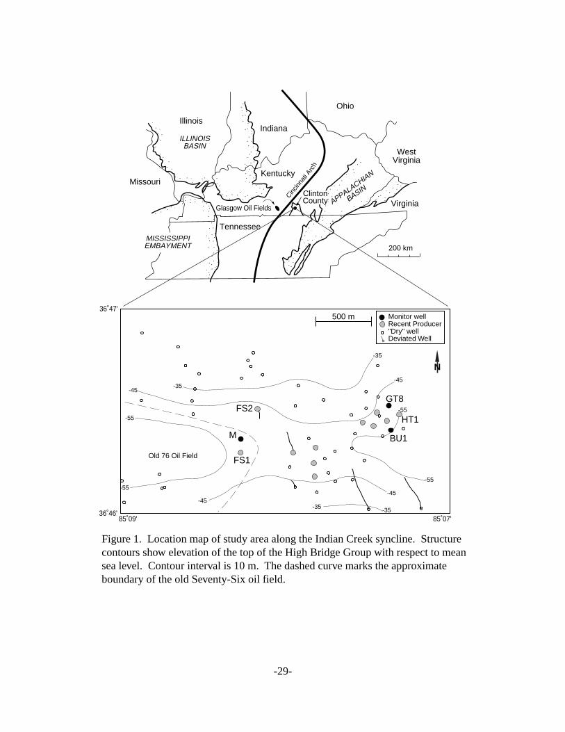
Figure 1. Location map of study area along the Indian Creek syncline. Structurecontours show elevation of the top of the High Bridge Group with respect to meansea level. Contour interval is 10 m. The dashed curve marks the approximate boundary of the old Seventy-Six oil field.

500 m

-35-45

-55

-55

-45-45

-35 -35

-55

-55

-45

-35

Old 76 Oil Field

FS2

M

FS1

BU1

HT1

GT8

36˚47'

36˚46'85˚09' 85˚07'

N

Monitor wellRecent Producer"Dry" wellDeviated Well

-30-

St. Louis, Warsaw & Fort PayneChattanooga ShaleCumberland, Leipers,and Clays Ferry

Lexington Limestone

High Bridge Group

Wells Creek DolomiteKnox Group

Mississippian

Geologic Period Formation

VelocityModel

Devonian

Upper and Middle Ordovician

Lower Ordovician

0

100

200

300

400

500

6005.5 6.0 6.5

km/s

Depth (m

)

Vp=6.04 km/s

Vs=2.93 km/s

Vp=6.37 km/s

Vs=2.95 km/s

Sonic Velocity

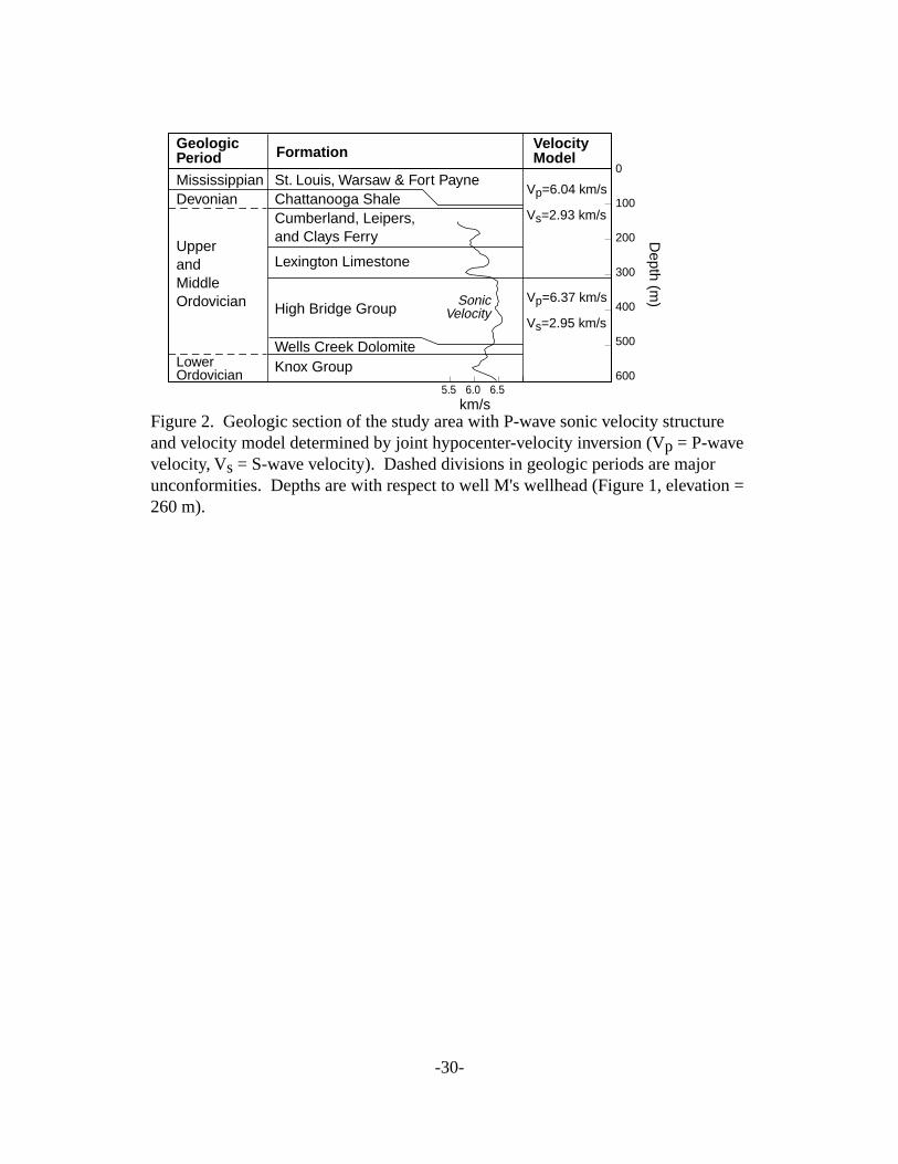
Figure 2. Geologic section of the study area with P-wave sonic velocity structureand velocity model determined by joint hypocenter-velocity inversion (Vp = P-wave velocity, Vs = S-wave velocity). Dashed divisions in geologic periods are majorunconformities. Depths are with respect to well M's wellhead (Figure 1, elevation =260 m).

-31-

0 0.1 0.2 0.3 0.4Time (sec)

V

H1

H2

P S

Figure 3. A representative microearthquake 3-component waveform recorded on the lowergeophone tool during FS2 monitoring (Table 1). V is the vertical component, H1 and H2 arethe two horizontal components. P- and S-wave arrivals are shown. All three traces areplotted at the same relative amplitude scale.

-32-

Cum

ulat

ive

Eve

nts

Cum

ulat

ive

Pro

duct

ion

(m3 )

Cum

ulat

ive

Pro

duct

ion

(m3 )

Cum

ulat

ive

Pro

duct

ion

(m3 )

140

120

100

80

60

40

20

1600

1400

1200

1000

800

600

400

200

0 2 4 6 8 10 12 14 16 18

0 2 4 6 8 10 12 14 16 18 20 22 24 26 28

Time (weeks)

1400

1200

1000

800

600

400

200

0

3500

3000

2500

2000

1500

1000

500

0 0

10

20

30

40

50

Cum

ulat

ive

Eve

nts

Cum

ulat

ive

Mo

(dyn

e-cm

)x10

17

FS1

FS2

HT1

(a)

(b)

(c)

Production

Production

Production

Events

Events

Events

Moment

Moment

Data Acquisiton off-line

0 2 4 6 8 10 12 14 16 18 20 22 24 26

20

0

3

6

9

12

15

40

60

80

100

120

140

160

180

2001800

1500

1200

900

600

300

Cum

ulat

ive

Eve

nts

Cum

ulat

ive

Mo

(dyn

e-cm

) x10

16

Figure 4. Cumulative production and number of events detected. (b) and (c) also showcumulative seismic moment (Mo). Week zero of all three plots marks the first day ofthe respective well's production history. Monitoring starts at the earliest position of thecumulative event curves shown for each test.

-33-

300 m A

B

N

OM3 OM1

OM2FS2

FS1

DD1

IW4

IW3IW2MF2

PD1 PD2

IW1GM3

MF1

M

Production Well

"Dry" Well

Monitor Well, M

group 1group 2group 3group 4no group

HypocenterSymbols

Figure 5. Map view of FS2 microearthquake hypocenters. Deviated welltrajectories have well symbols at wellhead locations.

-34-

0

150

300

450

600

Dep

th (

m)

A BPD1IW

2MF2

IW4

FS1MGM3

FS2

High Bridge Group

Knox Group

group 1group 2group 3group 4no group

Hypocenters

originalTD

Figure 6. Depth-section projection of FS2 hypocenters along profile A-B of Figure 5. Projection of production and monitor wells are also shown. Dashed horizontal lines markthe approximate tops of the High Bridge and Knox Groups. Depth is with respect to wellheadof M (elevation = 260 m). Well M is shown dashed from an obstruction at 378 m to its originalTD at 489 m. The square symbol along GM3 marks the depth at which brine was produced. No vertical exaggeration.

GeophoneProduction Zone✩

✩ ✩ ✩ ✩ ✩

1

23

4

-35-

0

150

300

450

600

Dep

th (

m)

N

PD1 IW2GM3 MF2

IW4

FS1 MFS2

150 m150 m

WHypocenter Groups

Group 1Group 2Group 3Group 4

produced brineOriginal TD

Figure 7. A perspective view of the fracture planes defined by FS2 hypocenter groups 1 through 4. The planar volumes were determined from the eigenvectors fitting thedistribution of microearthquake locations within each group. Dimensions of the planarvolumes exclude 10% of the extreme outer event locations in each dimension, so that outlying hypocenters do not affect the size and shape of the volumes defined by themajority of events. Hypocenters outside or near the boundaries of the planes are alsodisplayed. Well M is shown dashed from an obstruction at 378 m to its original TD at489 m. Production intervals are shown with horizontal bars along wellbore terminations.GM3 produced brine where it intersected the group 1 plane.

12

3

4

-36-

N 100 m GT8

BU1

Monitor well"Dry" wellProduction wellMicroearthquake

IW4

GT3

GT1GT10

GT2GT4

HT1

C1DD4

IW5

GT5

ET1

HW4

GTU9

B1

D

C

Figure 8. Map view of HT1 microearthquake hypocenters.

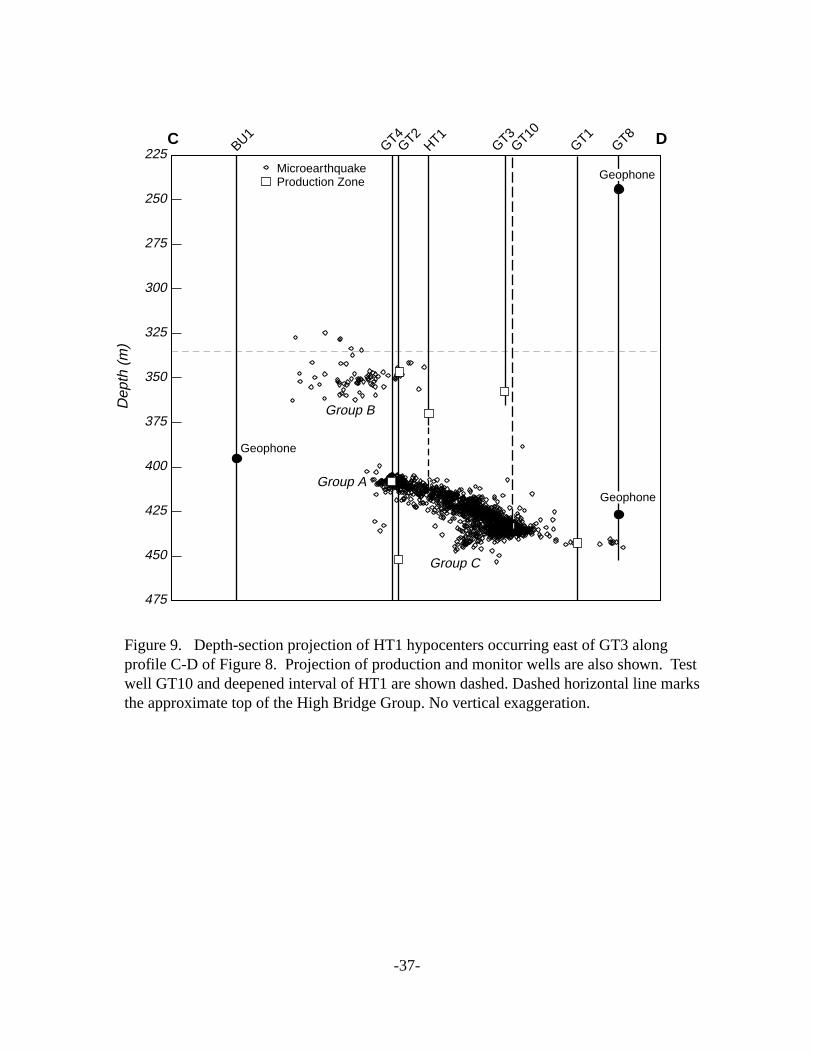
-37-

475

450

425

400

375

350

325

300

275

250

225

Dep

th (

m)

GT4BU1

GT2HT1

GT3GT10

GT1GT8C D

Geophone

Geophone

Geophone

Group B

Group A

Group C

Production ZoneMicroearthquake

Figure 9. Depth-section projection of HT1 hypocenters occurring east of GT3 alongprofile C-D of Figure 8. Projection of production and monitor wells are also shown. Testwell GT10 and deepened interval of HT1 are shown dashed. Dashed horizontal line marksthe approximate top of the High Bridge Group. No vertical exaggeration.

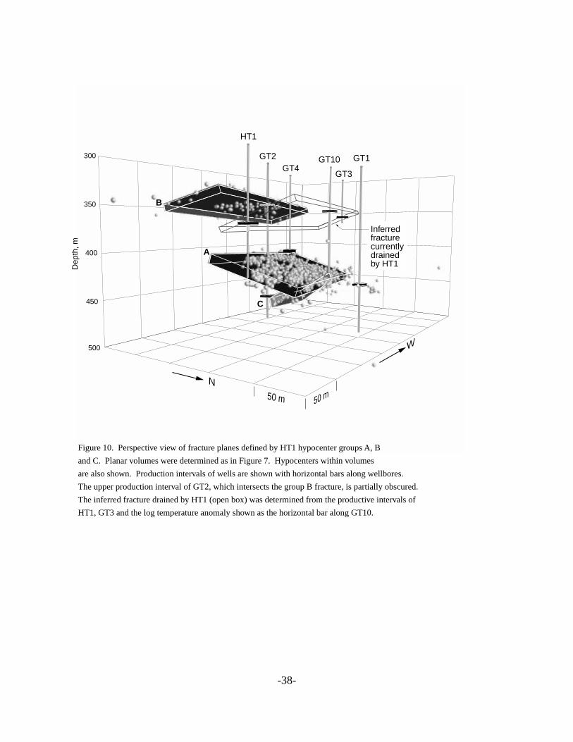
-38-

HT1

GT2GT4

GT10

GT3

GT1300

350

400

450

500

Dep

th, m

B

A

C

50 m 50 m

N

W

Inferredfracturecurrentlydrainedby HT1

Figure 10. Perspective view of fracture planes defined by HT1 hypocenter groups A, B

and C. Planar volumes were determined as in Figure 7. Hypocenters within volumes

are also shown. Production intervals of wells are shown with horizontal bars along wellbores.

The upper production interval of GT2, which intersects the group B fracture, is partially obscured.

The inferred fracture drained by HT1 (open box) was determined from the productive intervals of

HT1, GT3 and the log temperature anomaly shown as the horizontal bar along GT10.

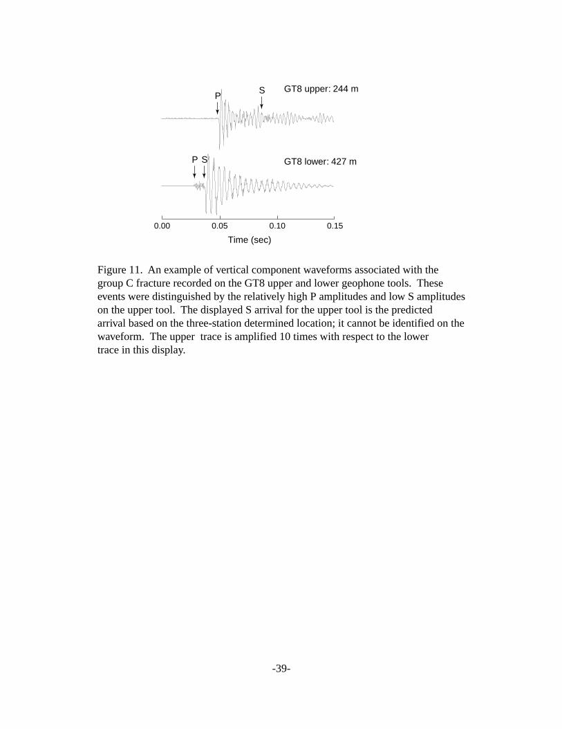
-39-

0.00 0.05 0.10 0.15

Time (sec)

GT8 upper: 244 m

GT8 lower: 427 mP

P

S

S

Figure 11. An example of vertical component waveforms associated with the group C fracture recorded on the GT8 upper and lower geophone tools. Theseevents were distinguished by the relatively high P amplitudes and low S amplitudeson the upper tool. The displayed S arrival for the upper tool is the predictedarrival based on the three-station determined location; it cannot be identified on thewaveform. The upper trace is amplified 10 times with respect to the lowertrace in this display.

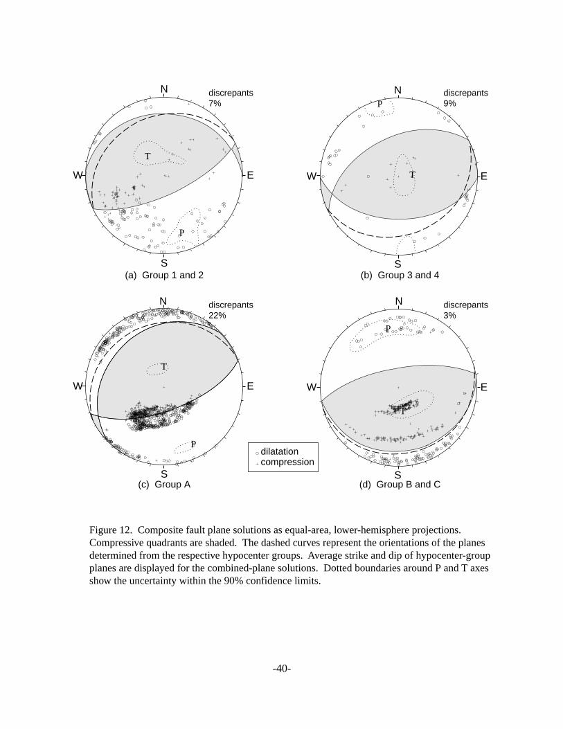
-40-

compressiondilatation

T

P

N

T

P

N

T

P

N

S S

W WE E

S S

W WE E

T

P

N

(a) Group 1 and 2 (b) Group 3 and 4

(c) Group A (d) Group B and C

discrepants7%

discrepants9%

discrepants22%

discrepants3%

Figure 12. Composite fault plane solutions as equal-area, lower-hemisphere projections.Compressive quadrants are shaded. The dashed curves represent the orientations of the planesdetermined from the respective hypocenter groups. Average strike and dip of hypocenter-groupplanes are displayed for the combined-plane solutions. Dotted boundaries around P and T axesshow the uncertainty within the 90% confidence limits.

-41-

Nσ1

σ2

σ3

Figure 13. Principle stress orientations determined from the composite focalmechanisms. Equal-area, lower-hemisphere projection.

-42-

500 m

-35-45

-55

-55

-45

-45

-35-35

-55

-55

-45

-35

FS2

BU1

FS1

36˚47'

36˚46'85˚09' 85˚07'

N

M

FS2 MicroearthquakesHT1 Microearthquakes

Monitor wellRecent Producer"Dry" well

Deviated Well

GT8

HT1

Old 76 Oil Field

Figure 14. Structure map of the top of High Bridge Group with FS2 and HT1 seismicity. Contoursshow elevation with respect to mean sea level at 10 m intervals. The dashed curve marks the approximate boundary of the old Seventy-Six oil field.

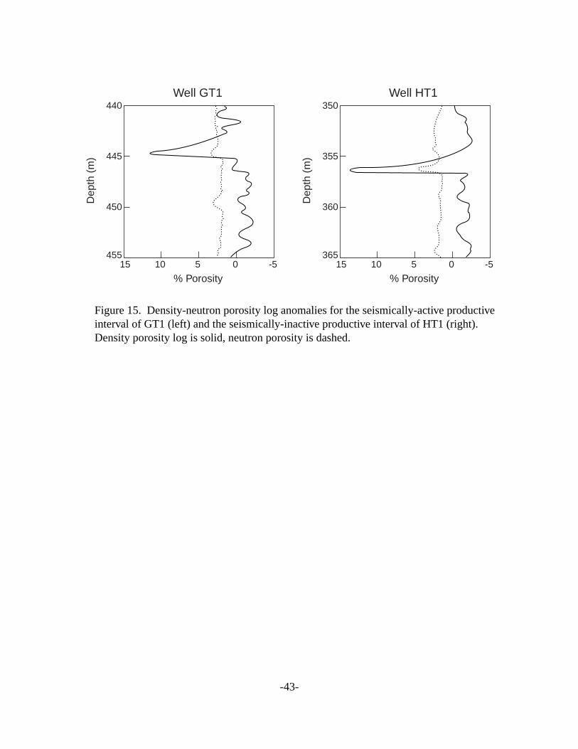
-43-

440

445

450

455

Dep

th (

m)

15 10 5 0 -5

% Porosity15 10 0 -5

% Porosity5

350

355

360

365

Dep

th (

m)

Well GT1 Well HT1

Figure 15. Density-neutron porosity log anomalies for the seismically-active productiveinterval of GT1 (left) and the seismically-inactive productive interval of HT1 (right). Density porosity log is solid, neutron porosity is dashed.

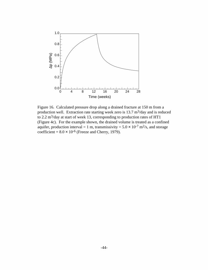
-44-

Time (weeks)0 4 8 12 16 20 24 28

∆p (

MP

a)

1.0

0.8

0.6

0.4

0.2

0.0

Figure 16. Calculated pressure drop along a drained fracture at 150 m from aproduction well. Extraction rate starting week zero is 13.7 m3/day and is reducedto 2.2 m3/day at start of week 13, corresponding to production rates of HT1(Figure 4c). For the example shown, the drained volume is treated as a confinedaquifer, production interval = 1 m, transmissivity = 5.0 × 10-7 m2/s, and storagecoefficient = 8.0 × 10-6 (Freeze and Cherry, 1979).