Fuel 116 (2014) 39–48

Contents lists available at ScienceDirect

Fuel

journal homepage: www.elsevier .com/locate / fuel

Reservoir oil viscosity determination using a rigorous approach

0016-2361/$ - see front matter � 2013 Elsevier Ltd. All rights reserved.http://dx.doi.org/10.1016/j.fuel.2013.07.072

⇑ Corresponding author at: Institut de Recherche en Génie Chimique et Pétrolier(IRGCP), Paris Cedex, France.

E-mail address: a.h.m@irgcp.fr (A.H. Mohammadi).

Abdolhossein Hemmati-Sarapardeh a, Amin Shokrollahi a, Afshin Tatar b, Farhad Gharagheizi c,d,Amir H. Mohammadi c,e,⇑, Ali Naseri f

a Department of Chemical and Petroleum Engineering, Sharif University of Technology, Tehran, Iranb Department of Chemical Engineering, Sahand University of Technology, Tabriz, Iranc Thermodynamics Research Unit, School of Chemical Engineering, University of KwaZulu-Natal, Howard College Campus, King George V Avenue, Durban 4041, South Africad Department of Chemical Engineering, Buinzahra Branch, Islamic Azad University, Buinzahra, Irane Institut de Recherche en Génie Chimique et Pétrolier (IRGCP), Paris Cedex, Francef EOR Department, Research Institute of Petroleum Industry (RIPI), Tehran, Iran

h i g h l i g h t s

� Reliable viscosity models for oil systems have been developed.� A large database consisting of over 1000 data have been used to develop them.� Their reliability is successfully examined against independent data.

a r t i c l e i n f o

Article history:Received 26 November 2012Received in revised form 14 April 2013Accepted 18 July 2013Available online 2 August 2013

Keywords:Crude oil viscosityModelReservoir fluidPVTSupport vector machine

a b s t r a c t

Viscosity of crude oil is a fundamental factor in simulating reservoirs, forecasting production as well asplanning thermal enhanced oil recovery methods which make its accurate determination necessary.Experimental determination of reservoir oil viscosity is costly and time consuming. Hence, searchingfor quick and accurate determination of reservoir oil viscosity is inevitable. The objective of this studyis to present a reliable, and predictive model namely, Least-Squares Support Vector Machine (LSSVM)to predict reservoir oil viscosity. To this end, three LSSVM models have been developed for predictionof reservoir oil viscosity in the three regions including, under-saturated, saturated and dead oil. Thesemodels have been developed and tested using more than 1000 series of experimental PVT data of Iranianoil reservoirs. These data include oil API gravity, reservoir temperature, solution gas oil ratio, and satura-tion pressure. The ranges of data used to develop these new models cover almost all Iranian oil reservoirsPVT data and consequently the developed models could be reliable for prediction of other Iranian oil res-ervoirs viscosities. In-depth comparative studies have been carried out between these new models andthe most frequently used oil viscosity correlations for prediction of reservoir oil viscosity. The resultsshow that the developed LSSVM models significantly outperform the existing correlations and providepredictions in acceptable agreement with experimental data. Furthermore, it is shown that the proposedmodels are capable of simulating the actual physical trend of the oil viscosity with variation of oil APIgravity, temperature, and pressure.

� 2013 Elsevier Ltd. All rights reserved.

1. Introduction

Viscosity of crude oil is an important parameter for evaluatingperformance of the reservoir, reservoir simulation, designing pro-duction facilities and utilizing the best scenario for production[1–5]. Hence, accurate determination of this parameter is crucialfor the petroleum industry. The common approach to determinethe viscosity is laboratory analysis on the bottomhole samples or

recombined liquids and gases collected from the separators atthe surface. When PVT data are not available, in order to save timeand cost, fluid properties are determined by empirical correlationsand equations of state (EOS).

Depending on the input variables, it is possible to divide corre-lations used for determining oil viscosity in two classes [4]: Thefirst class uses common oil field data such as reservoir tempera-ture, saturation pressure, oil API gravity, and solution gas oil ratio.The second one is empirical or semi-empirical models that usesome characteristics not used in the first approach such as reser-voir fluid composition, critical temperature, acentric factor, pourpoint temperature, molar mass, and normal boiling point [6–8].

Nomenclature

AARD Average Absolute Relative DeviationsAPI oil API gravityEi percent relative errorGOR gas oil ratio, SCF/STBLSSVM Least-Squares Supported Vector MachineN number of data pointsP pressure, MPaPb bubble point pressure, MPaR2 squared correlation coefficientsRMSE Root Mean Square Error

SCF standard cubic feetSTB standard tank barrelSTD Standard Deviation ErrorsT temperature, Klo oil viscosity, cPlob bubble point oil viscosity, cPlod dead oil viscosity, cP

40 A. Hemmati-Sarapardeh et al. / Fuel 116 (2014) 39–48

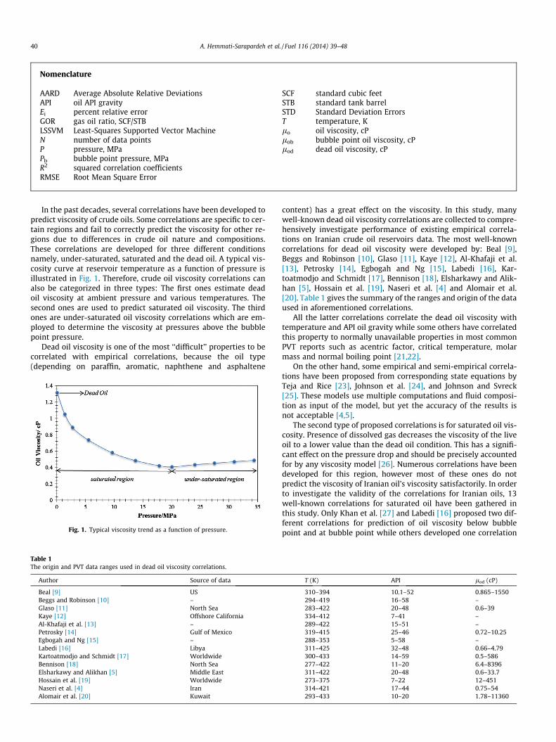
In the past decades, several correlations have been developed topredict viscosity of crude oils. Some correlations are specific to cer-tain regions and fail to correctly predict the viscosity for other re-gions due to differences in crude oil nature and compositions.These correlations are developed for three different conditionsnamely, under-saturated, saturated and the dead oil. A typical vis-cosity curve at reservoir temperature as a function of pressure isillustrated in Fig. 1. Therefore, crude oil viscosity correlations canalso be categorized in three types: The first ones estimate deadoil viscosity at ambient pressure and various temperatures. Thesecond ones are used to predict saturated oil viscosity. The thirdones are under-saturated oil viscosity correlations which are em-ployed to determine the viscosity at pressures above the bubblepoint pressure.

Dead oil viscosity is one of the most ‘‘difficult’’ properties to becorrelated with empirical correlations, because the oil type(depending on paraffin, aromatic, naphthene and asphaltene

Fig. 1. Typical viscosity trend as a function of pressure.

Table 1The origin and PVT data ranges used in dead oil viscosity correlations.

Author Source of data

Beal [9] USBeggs and Robinson [10] –Glaso [11] North SeaKaye [12] Offshore CaliforniaAl-Khafaji et al. [13] –Petrosky [14] Gulf of MexicoEgbogah and Ng [15] –Labedi [16] LibyaKartoatmodjo and Schmidt [17] WorldwideBennison [18] North SeaElsharkawy and Alikhan [5] Middle EastHossain et al. [19] WorldwideNaseri et al. [4] IranAlomair et al. [20] Kuwait

content) has a great effect on the viscosity. In this study, manywell-known dead oil viscosity correlations are collected to compre-hensively investigate performance of existing empirical correla-tions on Iranian crude oil reservoirs data. The most well-knowncorrelations for dead oil viscosity were developed by: Beal [9],Beggs and Robinson [10], Glaso [11], Kaye [12], Al-Khafaji et al.[13], Petrosky [14], Egbogah and Ng [15], Labedi [16], Kar-toatmodjo and Schmidt [17], Bennison [18], Elsharkawy and Alik-han [5], Hossain et al. [19], Naseri et al. [4] and Alomair et al.[20]. Table 1 gives the summary of the ranges and origin of the dataused in aforementioned correlations.

All the latter correlations correlate the dead oil viscosity withtemperature and API oil gravity while some others have correlatedthis property to normally unavailable properties in most commonPVT reports such as acentric factor, critical temperature, molarmass and normal boiling point [21,22].

On the other hand, some empirical and semi-empirical correla-tions have been proposed from corresponding state equations byTeja and Rice [23], Johnson et al. [24], and Johnson and Svreck[25]. These models use multiple computations and fluid composi-tion as input of the model, but yet the accuracy of the results isnot acceptable [4,5].

The second type of proposed correlations is for saturated oil vis-cosity. Presence of dissolved gas decreases the viscosity of the liveoil to a lower value than the dead oil condition. This has a signifi-cant effect on the pressure drop and should be precisely accountedfor by any viscosity model [26]. Numerous correlations have beendeveloped for this region, however most of these ones do notpredict the viscosity of Iranian oil’s viscosity satisfactorily. In orderto investigate the validity of the correlations for Iranian oils, 13well-known correlations for saturated oil have been gathered inthis study. Only Khan et al. [27] and Labedi [16] proposed two dif-ferent correlations for prediction of oil viscosity below bubblepoint and at bubble point while others developed one correlation

T (K) API lod (cP)

310–394 10.1–52 0.865–1550294–419 16–58 –283–422 20–48 0.6–39334–412 7–41 –289–422 15–51 –319–415 25–46 0.72–10.25288–353 5–58 –311–425 32–48 0.66–4.79300–433 14–59 0.5–586277–422 11–20 6.4–8396311–422 20–48 0.6–33.7273–375 7–22 12–451314–421 17–44 0.75–54293–433 10–20 1.78–11360

Table 2The origin and PVT data ranges used in saturated oil viscosity correlations.

Author Source of data Solution GOR (SCF/STB) Saturation pressure (MPa) lo (cP)

Chew and Connally 1 [28] US 51–3544 0.91–38.92 0.37–50Chew and Connally 2 [28] US 51–3544 0.91–38.92 0.37–50Chew and Connally 3 [28] US 51–3544 0.91–38.92 0.37–50Beggs and Robinson [10] – 20–2070 0.91–36.30 –Al-Khafaji et al. [13] – 0–2100 – –Khan et al. [27] Saudi Arabia 24–1901 0.74–29.75 0.13–77.4Petrosky [14] Gulf of Mexico 21–1855 10.85–65.85 0.21–7.4Labedi [16] Libya 13–3533 0.41–43.83 0.115–3.72Kartoatmodjo and Schmidt [17] Worldwide 2.3–572 0.10–41.74 0.1–6.3Elsharkawy and Alikhan [5] Middle East 10–3600 0.69–25.51 0.05–21Hossain et al. [19] Worldwide 19–493 0.83–43.24 3.6–360Naseri et al. [4] Iran 255–4116 2.89–40.68 0.11–18.15Bergman and Sutton [26] Worldwide 6–6525 0.45–71.02 0.21–4277

A. Hemmati-Sarapardeh et al. / Fuel 116 (2014) 39–48 41

for saturated oil. Some correlations consider saturated oil viscosityas a function of dead oil viscosity and solution gas oil ratio and theothers introduce it as a function of dead oil viscosity and saturationpressure. Available correlations in literature are Chew andConnally 1 [28], Chew and Connally 2 [28], Chew and Connally 3[28], Beggs and Robinson [10], Al-Khafaji et al. [13], Khan et al.[27], Petrosky [14], Labedi [16], Kartoatmodjo and Schmidt [17],Elsharkawy and Alikhan [5], Hossain et al. [19], Naseri et al. [4],and Bergman and Sutton [26]. Table 2 illustrates the origin andranges of the data used in the aforementioned correlations.

The last type is under-saturated oil viscosity correlations. Sincethe solution gas oil ratio is constant in this region, pressure is themain parameter that controls viscosity. Lots of models are pro-posed for prediction of viscosity in this region [5,9,14,16,17,19,27,29–35]. Some of these correlations regard the viscosity as afunction of pressure, bubble point pressure, and bubble point oilviscosity, while the others additionally have involved API oil grav-ity and dead oil viscosity at their correlations [5,16]. Available cor-relations for under-saturated oil viscosity are: Beal [9], Vazquezand Beggs [35], Khan et al. [27], Petrosky [14], Labedi [16], Orbeyand Sandler [32], Kartoatmodjo and Schmidt [17], Elsharkawyand Alikhan [5], and Hossain et al. [19]. The summery of the origin

Table 3The origin and PVT data ranges used in under-saturated oil viscosity correlations.

Author Source of data P (MPa)

Beal [9] US –Vazquez and Beggs [35] Worldwide 0.87–65.50Khan et al. [27] Saudi Arabia –Petrosky [14] Gulf of Mexico 11.03–70.67Labedi [16] Libya –Orbey and Sandler [32] – 5.10–100.00Kartoatmodjo and Schmidt [17] Worldwide 0.17–41.47Elsharkawy and Alikhan [5] Middle East 8.87–68.94Hossain et al. [19] Worldwide 2.07–23.44

Table 4Ranges and their corresponding statistical parameters of the input/output data used for d

Model Parameter M

Dead oil Temperature (K) 2Oil gravity (API)Dead oil viscosity (cP)

Saturated oil viscosity Saturation pressure (MPa)Dead oil viscosity (cP)Saturated oil viscosity (cP)

Under-saturated oil viscosity Bubble point pressure (MPa)Bubble point viscosity (cP)Pressure (MPa)Under-saturated oilviscosity (cP)

and ranges of the data used in the aforementioned correlations arepresented in Table 3.

The aim of the present study is to develop a novel model,namely Least Squares Supported Vector Machine (LSSVM) [36]for predicting the oil viscosity. For this purpose, based on morethan 1000 Iranian oil reservoirs data, three new models are pro-posed for prediction of the under-saturated, saturated and deadoil viscosities. A quantitative and qualitative analysis of the modelis carried out to establish the adequacy and accuracy of the model.In addition, in order to evaluate the performance of the newly pro-posed models against the other ones, both statistical and graphicalerror analyses are utilized simultaneously.

2. Model development

2.1. Database

Reliability of the models for prediction of properties and phasebehaviors of fluids generally depends on the comprehensiveness ofthe employed dataset for their development [37–42]. Hence, morethan 1000 series of experimental PVT data of Iranian oil reservoirs

Pb (MPa) lob (cP) lo (cP)

– 0.142–127 0.16–315– – 0.117–1480.74–33.05 0.13–77.4 0.13–7110.85–65.86 0.211–3.546 0.22–4.090.41–43.84 0.115–3.72 –– 0.217–3.1 0.225–7.30.17–32.92 0.168–184.86 0.168–517.03– – 0.2–5.70.83–43.24 3.6–360 3–517

eveloping the models.

inimum Maximum Average Standard deviation

83.15 416.48 353.06 42.8417.30 43.56 29.32 7.00

0.39 69.50 7.41 11.44

1.09 39.31 11.76 7.500.55 37.18 4.55 5.050.18 25.58 1.92 2.59

5.03 35.27 17.56 7.810.18 18.16 1.62 2.195.03 86.18 25.38 11.630.18 31.00 1.84 2.97

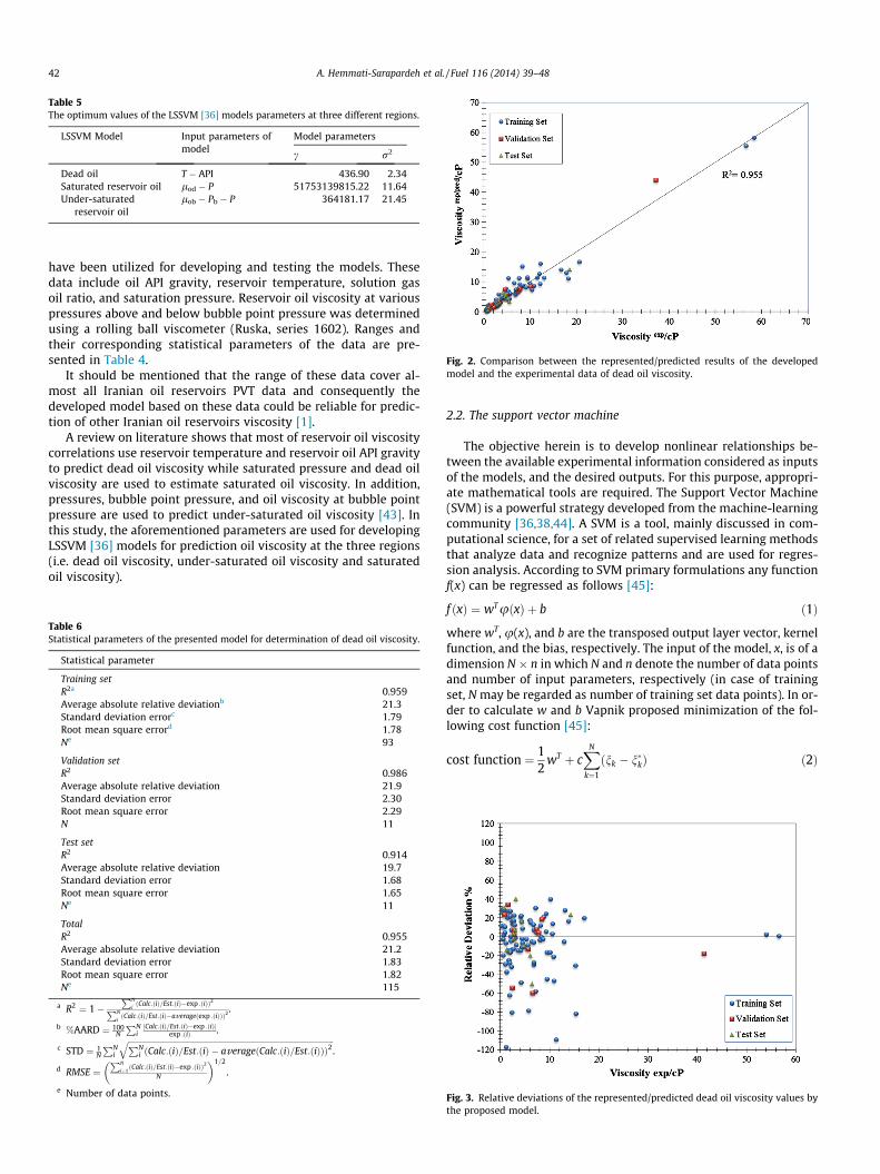
Fig. 2. Comparison between the represented/predicted results of the developedmodel and the experimental data of dead oil viscosity.

Table 5The optimum values of the LSSVM [36] models parameters at three different regions.

LSSVM Model Input parameters ofmodel

Model parameters

c r2

Dead oil T � API 436.90 2.34Saturated reservoir oil lod � P 51753139815.22 11.64Under-saturated

reservoir oillob � Pb � P 364181.17 21.45

42 A. Hemmati-Sarapardeh et al. / Fuel 116 (2014) 39–48

have been utilized for developing and testing the models. Thesedata include oil API gravity, reservoir temperature, solution gasoil ratio, and saturation pressure. Reservoir oil viscosity at variouspressures above and below bubble point pressure was determinedusing a rolling ball viscometer (Ruska, series 1602). Ranges andtheir corresponding statistical parameters of the data are pre-sented in Table 4.

It should be mentioned that the range of these data cover al-most all Iranian oil reservoirs PVT data and consequently thedeveloped model based on these data could be reliable for predic-tion of other Iranian oil reservoirs viscosity [1].

A review on literature shows that most of reservoir oil viscositycorrelations use reservoir temperature and reservoir oil API gravityto predict dead oil viscosity while saturated pressure and dead oilviscosity are used to estimate saturated oil viscosity. In addition,pressures, bubble point pressure, and oil viscosity at bubble pointpressure are used to predict under-saturated oil viscosity [43]. Inthis study, the aforementioned parameters are used for developingLSSVM [36] models for prediction oil viscosity at the three regions(i.e. dead oil viscosity, under-saturated oil viscosity and saturatedoil viscosity).

Table 6Statistical parameters of the presented model for determination of dead oil viscosity.

Statistical parameter

Training setR2a 0.959Average absolute relative deviationb 21.3Standard deviation errorc 1.79Root mean square errord 1.78Ne 93

Validation setR2 0.986Average absolute relative deviation 21.9Standard deviation error 2.30Root mean square error 2.29N 11

Test setR2 0.914Average absolute relative deviation 19.7Standard deviation error 1.68Root mean square error 1.65Ne 11

TotalR2 0.955Average absolute relative deviation 21.2Standard deviation error 1.83Root mean square error 1.82Ne 115

a R2 ¼ 1�PN

iðCalc:ðiÞ=Est:ðiÞ�exp :ðiÞÞ2PN

iðCalc:ðiÞ=Est:ðiÞ�averageðexp :ðiÞÞÞ2

.

b %AARD ¼ 100N

PNijCalc:ðiÞ=Est:ðiÞ�exp :ðiÞj

exp :ðiÞ .

c STD ¼ 1N

PNi

ffiffiffiffiffiffiffiffiffiffiffiffiffiffiffiffiffiffiffiffiffiffiffiffiffiffiffiffiffiffiffiffiffiffiffiffiffiffiffiffiffiffiffiffiffiffiffiffiffiffiffiffiffiffiffiffiffiffiffiffiffiffiffiffiffiffiffiffiffiffiffiffiffiffiffiffiffiffiffiffiffiffiffiffiffiffiffiffiffiffiffiffiffiffiffiffiffiffiffiffiffiffiPNi ðCalc:ðiÞ=Est:ðiÞ � averageðCalc:ðiÞ=Est:ðiÞÞÞ2

q.

d RMSE ¼PN

i¼1ðCalc:ðiÞ=Est:ðiÞ�exp :ðiÞÞ2

N

� �1=2

.

e Number of data points.

2.2. The support vector machine

The objective herein is to develop nonlinear relationships be-tween the available experimental information considered as inputsof the models, and the desired outputs. For this purpose, appropri-ate mathematical tools are required. The Support Vector Machine(SVM) is a powerful strategy developed from the machine-learningcommunity [36,38,44]. A SVM is a tool, mainly discussed in com-putational science, for a set of related supervised learning methodsthat analyze data and recognize patterns and are used for regres-sion analysis. According to SVM primary formulations any functionf(x) can be regressed as follows [45]:

f ðxÞ ¼ wTuðxÞ þ b ð1Þ

where wT, u(x), and b are the transposed output layer vector, kernelfunction, and the bias, respectively. The input of the model, x, is of adimension N � n in which N and n denote the number of data pointsand number of input parameters, respectively (in case of trainingset, N may be regarded as number of training set data points). In or-der to calculate w and b Vapnik proposed minimization of the fol-lowing cost function [45]:

cost function ¼ 12

wT þ cXN

k¼1

ðnk � n�kÞ ð2Þ

Fig. 3. Relative deviations of the represented/predicted dead oil viscosity values bythe proposed model.

Table 7Comparison between the performances of LSSVM [36] model and common correla-tions for prediction of dead oil viscosity.

Author AARD, % R2 RMSE

Beal [9] 891 0.1088 83.14Beggs and Robinson [10] 217 0.0376 245.05Glaso [11] 33.41 0.9270 3.84Kaye [12] 52.05 0.2268 10.19Al-Khafaji et al. [13] 29.97 0.7283 6.04Petrosky [14] 41.62 0.8695 4.18Egbogah and Ng [15] 55.60 0.9208 3.26Labedi [16] 178 0.3910 14.95Kartoatmodjo and Schmidt [17] 36.89 0.9065 4.50Bennison [18] 70.97 0.6689 12.25Elsharkawy and Alikhan [5] 72.92 0.9065 13.25Hossain et al. [19] 68.92 0.6000 16.24Naseri et al. [4] 27.57 0.8233 3.88Alomair et al. [20] 72.42 0.8275 6.36LSSVM Model (this study) 21.2 0.955 1.82

Fig. 4. Trend of dead oil viscosity changes versus oil API gravity at differentisotherms (this study).

Fig. 5. Comparison between the represented/predicted results of the developedmodel and the experimental data of saturated oil viscosity.

Fig. 6. Relative deviations of the represented/predicted saturated oil viscosityvalues by proposed model.

Table 8Statistical parameters of the presented model for determination of saturated oilviscosity.

Statistical parameter

Training setR2 0.988Average absolute relative deviation 13.5Standard deviation error 0.31Root mean square error 0.31N 323

Validation setR2 0.976Average absolute relative deviation 13.6Standard deviation error 0.24Root mean square error 0.24N 40

Test setR2 0.838Average absolute relative deviation 13.2Standard deviation error 0.77Root mean square error 0.77N 40

TotalR2 0.979Average absolute relative deviation 14.6Standard deviation error 0.38Root mean square error 0.38N 403

Table 9Comparison between the performances of LSSVM [36] model and common correla-tions for prediction of saturated oil viscosity.

Author AARD (%) R2 RMSE

Chew and Connally 1 [28] 29.64 0.823818 1.18Chew and Connally 2 [28] 39.64 0.799963 1.46Chew and Connally 3 [28] Out of range 0 Out of rangeBeggs and Robinson [10] 31.90 0.532063 1.35Al-Khafaji et al. [13] 20.79 0.799255 1.32Khan et al. [27] Out of range 0 Out of rangePetrosky [14] 27.33 0.739977 1.14Labedi [16] 249 0.428383 3.70Kartoatmodjo and Schmidt [17] 25.71 0.789565 1.11Elsharkawy and Alikhan [5] 24.45 0.657688 1.20Hossain et al. [19] Out of range 0 Out of rangeNaseri et al. [4] 52.32 0.567231 1.38Bergman and Sutton [26] 26.70 0.733941 1.15LSSVM Model (this study) 14.6 0.979 0.38

A. Hemmati-Sarapardeh et al. / Fuel 116 (2014) 39–48 43

Subjected to the following constraint:

yk �wTuðxkÞ � b 6 eþ nk; k ¼ 1;2; . . . ;N

wTuðxkÞ þ b� yk 6 eþ n�k; k ¼ 1;2; . . . ;N

nk; n�k 6 0; k ¼ 1;2; . . . ;N

8><>: ð3Þ

where xk and yk are kth data point input and kth data pointoutput, respectively. The e is the fixed precision of the function

Fig. 7. Comparison between experimental data and predicted values provided bynew proposed LSSVM [36] model for reservoir oil viscosity of four saturatedsamples .

Table 10Statistical parameters of the presented model for determination of under-saturatedoil viscosity.

Statistical parameter

Training setR2 0.999Average absolute relative deviation 1.5Standard deviation error 0.03Root mean square error 0.03N 418

Validation setR2 0.999Average absolute relative deviation 1.3Standard deviation error 0.05Root mean square error 0.05N 52

Test setR2 0.999Average absolute relative deviation 1.4Standard deviation error 0.04Root mean square error 0.04N 52

TotalR2 0.999Average absolute relative deviation 1.4Standard deviation error 0.04Root mean square error 0.04N 522

44 A. Hemmati-Sarapardeh et al. / Fuel 116 (2014) 39–48

approximation. The nk and n�k are slack variables. It is obvious thatwhen we choose a small e to develop a very accurate model, somedata points may be outside of the e precision. This may result ininfeasible solution. Therefore, we should use slack parameters todefine the allowed margin of error. The c > 0 is the tuning parameterof the SVM which determines the amount of the deviation from thedesired e. In other words, c is one of the tuning parameters of theSVM. In order to minimize the cost function depicted in Eq. (2)along with its constraints presented in Eq. (3), we should use theLagrangian for this problem as follows [45]:

Lða; a�Þ ¼ �12

XN

k;l¼1

ðak � a�kÞðal � a�l ÞKðxk; xlÞ � eXN

k¼1

ðak � a�kÞ

þXN

k¼1

ykðak � a�kÞ ð4Þ

Fig. 8. Percent relative error distribution of the most accurate satur

XN

k¼1

ðak � a�kÞ ¼ 0; ak; a�k 2 ½0; c� ð4aÞ

Kðxk; xlÞ ¼ uðxkÞTuðxlÞ; k ¼ 1;2; . . . ;N ð4bÞ

where ak and a�k are Lagrangin multipliers. Finally, the final form ofthe SVM is obtained as follows:

ated oil viscosity correlations and proposed LSSVM [36] model.

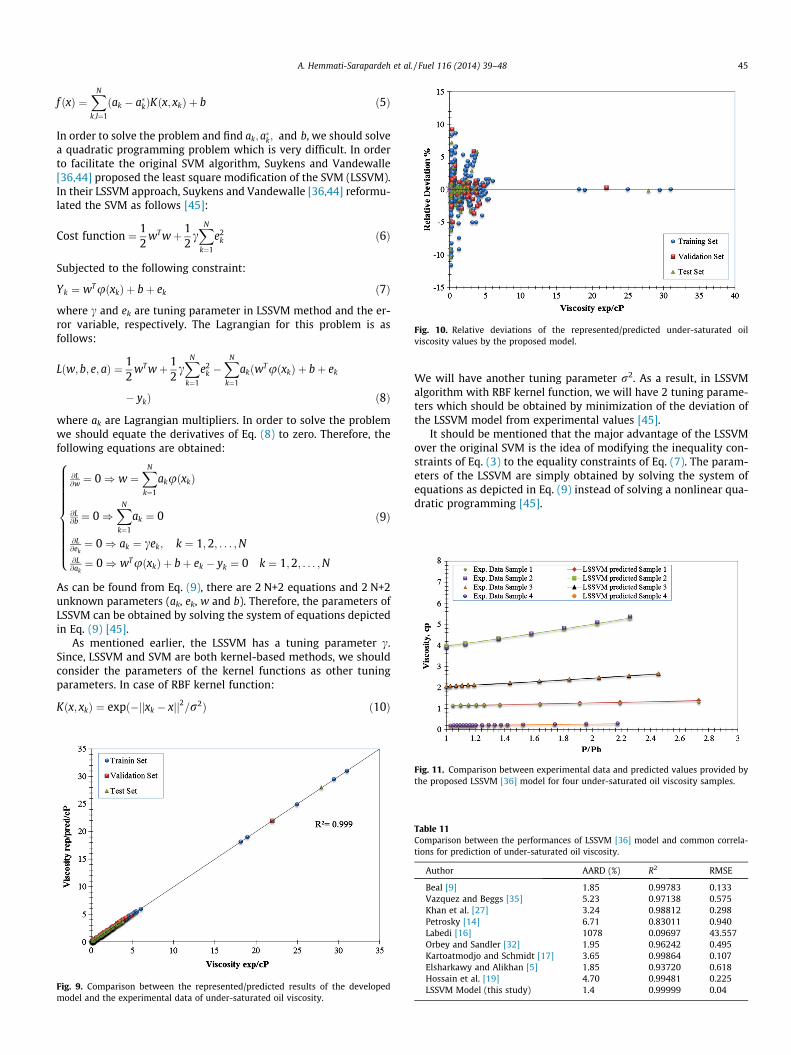
Fig. 10. Relative deviations of the represented/predicted under-saturated oilviscosity values by the proposed model.

A. Hemmati-Sarapardeh et al. / Fuel 116 (2014) 39–48 45

f ðxÞ ¼XN

k;l¼1

ðak � a�kÞKðx; xkÞ þ b ð5Þ

In order to solve the problem and find ak; a�k; and b, we should solvea quadratic programming problem which is very difficult. In orderto facilitate the original SVM algorithm, Suykens and Vandewalle[36,44] proposed the least square modification of the SVM (LSSVM).In their LSSVM approach, Suykens and Vandewalle [36,44] reformu-lated the SVM as follows [45]:

Cost function ¼ 12

wT wþ 12cXN

k¼1

e2k ð6Þ

Subjected to the following constraint:

Yk ¼ wTuðxkÞ þ bþ ek ð7Þ

where c and ek are tuning parameter in LSSVM method and the er-ror variable, respectively. The Lagrangian for this problem is asfollows:

Lðw; b; e; aÞ ¼ 12

wT wþ 12cXN

k¼1

e2k �

XN

k¼1

akðwTuðxkÞ þ bþ ek

� ykÞ ð8Þ

where ak are Lagrangian multipliers. In order to solve the problemwe should equate the derivatives of Eq. (8) to zero. Therefore, thefollowing equations are obtained:

@L@w ¼ 0) w ¼

XN

k¼1

akuðxkÞ

@L@b ¼ 0)

XN

k¼1

ak ¼ 0

@L@ek¼ 0) ak ¼ cek; k ¼ 1;2; . . . ;N

@L@ak¼ 0) wTuðxkÞ þ bþ ek � yk ¼ 0 k ¼ 1;2; . . . ;N

8>>>>>>>>>><>>>>>>>>>>:

ð9Þ

As can be found from Eq. (9), there are 2 N+2 equations and 2 N+2unknown parameters (ak, ek, w and b). Therefore, the parameters ofLSSVM can be obtained by solving the system of equations depictedin Eq. (9) [45].

As mentioned earlier, the LSSVM has a tuning parameter c.Since, LSSVM and SVM are both kernel-based methods, we shouldconsider the parameters of the kernel functions as other tuningparameters. In case of RBF kernel function:

Kðx; xkÞ ¼ expð�jjxk � xjj2=r2Þ ð10Þ

Fig. 9. Comparison between the represented/predicted results of the developedmodel and the experimental data of under-saturated oil viscosity.

We will have another tuning parameter r2. As a result, in LSSVMalgorithm with RBF kernel function, we will have 2 tuning parame-ters which should be obtained by minimization of the deviation ofthe LSSVM model from experimental values [45].

It should be mentioned that the major advantage of the LSSVMover the original SVM is the idea of modifying the inequality con-straints of Eq. (3) to the equality constraints of Eq. (7). The param-eters of the LSSVM are simply obtained by solving the system ofequations as depicted in Eq. (9) instead of solving a nonlinear qua-dratic programming [45].

Fig. 11. Comparison between experimental data and predicted values provided bythe proposed LSSVM [36] model for four under-saturated oil viscosity samples.

Table 11Comparison between the performances of LSSVM [36] model and common correla-tions for prediction of under-saturated oil viscosity.

Author AARD (%) R2 RMSE

Beal [9] 1.85 0.99783 0.133Vazquez and Beggs [35] 5.23 0.97138 0.575Khan et al. [27] 3.24 0.98812 0.298Petrosky [14] 6.71 0.83011 0.940Labedi [16] 1078 0.09697 43.557Orbey and Sandler [32] 1.95 0.96242 0.495Kartoatmodjo and Schmidt [17] 3.65 0.99864 0.107Elsharkawy and Alikhan [5] 1.85 0.93720 0.618Hossain et al. [19] 4.70 0.99481 0.225LSSVM Model (this study) 1.4 0.99999 0.04

46 A. Hemmati-Sarapardeh et al. / Fuel 116 (2014) 39–48

2.3. Computational procedure

In the next step, the database is divided into three sub data setsincluding the ‘‘Training’’ set, the ‘‘Optimization’’ set, and the ‘‘Test’’set. Generally, the ‘‘Training’’ set is used to generate the modelstructure, the ‘‘Optimization’’ set is applied for optimization ofthe model and the ‘‘Test (prediction)’’ set is used to investigateits prediction capability and validity [37–39,46]. The databasewas split randomly into three sub data sets: For this purpose, about80%, 10%, and 10% of the main data set were randomly selected forthe ‘‘Training’’ set, the ‘‘Optimization’’ set, and the ‘‘Test’’ set,respectively. The effect of the percent allocation of the three subdata sets from the database on the accuracy of the final modelhas been studied elsewhere [37,39]. In distribution of the datathrough the three sub data sets, we generally perform many distri-butions to avoid the local accumulations of the data in the feasibleregion of the problem. As a result, the acceptable distribution is theone with homogeneous accumulations of the data on the domainof the three sub data sets [39].

3. Results and discussion

In this study, three LSSVM [36] models were developed to pre-dict the viscosity of dead oil, saturated reservoir oil and under-sat-urated reservoir oil, as mentioned earlier. Furthermore, predictionperformance of the newly proposed models was compared againstall well-known previously published correlations by means of sta-tistical and graphical error analyses.

The values of the probable global optima of all three modelsincluding r2 and c are reported in Table 5. It should be stated thatdetermination of these values are not generally simple and thenumbers of the reported digits are normally obtained by sensitivityanalysis of the overall errors of the optimization procedure to thecorresponding values [37,47]. Furthermore, Simulating Annealing(SA) technique was applied in this study [48,49].

Table 6 indicates the statistical parameters of the proposedmodel for prediction of dead oil viscosity, including Average Abso-lute Relative Deviations (AARD), Root Mean Square Errors (RMSE),

Fig. 12. Percent relative error distribution of the most accurate under-sat

squared correlation coefficients (R2), and Standard Deviation Errors(STD). A comparison between the predicted dead oil viscosity val-ues and the experimental values and relative error distribution forexperimental data points are demonstrated in Figs. 2 and 3,respectively.

To investigate the validity of the proposed LSSVM [36] modelfor dead oil viscosity, all previously published correlations havebeen selected for comparison. As mentioned earlier, dead oil vis-cosity is generally a ‘‘difficult’’ property to be correlated. Table 7shows the results of all the correlations compared to the LSSVM[36] model. According to this table, the developed model givesan AARD of 21.2%, R2 of 0.955, and RMSE of 1.82.

Fig. 4 shows the trend of changes in dead oil viscosity withincreasing API gravity of oil at various temperatures. As a generalrule, dead oil viscosity decreases with an increase in the oil APIgravity [50,51]. Furthermore, a general reduction in dead oil vis-cosity is expected with increasing temperature, and this effect ismore sensible at lower temperatures [50,51]. As can be seen fromFig. 4, this trend is captured by the proposed LSSVM [36] model fordead oil viscosity.

Next model was developed for estimation of saturated reservoiroil viscosity. Comparison between the results of predictions madeby proposed LSSVM [36] model, and the corresponding experimen-tal viscosity values for saturated reservoir oil is illustrated in Fig. 5.Furthermore, Fig. 6 shows relative error distribution of proposedmodel. Its statistical parameters for prediction of saturated reser-voir oil viscosity are reported in Table 8.

The efficiency of the model for saturated oil viscosity was alsotested against all well-known correlations and results are dis-played in Table 9. According to this table the values of AARD, R2,and RMSE are 14.6%, 0.979, and 0.38 respectively. Statistical andgraphical error analysis demonstrate that the proposed LSSVM[36] model outperforms previously published correlations .

To make sure that the proposed model is reliable, the validity ofmodel should be checked. For this purpose, the resulted trend fromthe proposed model [36] was checked by four experimental datasamples. Fig. 7 demonstrates experimental and predicted viscosi-ties made by the new LSSVM [36] model for four samples. It is

urated oil viscosity correlations and the proposed LSSVM [36] model.

A. Hemmati-Sarapardeh et al. / Fuel 116 (2014) 39–48 47

evident by increasing pressure ultimately to the bubble point pres-sure, viscosity of saturated reservoir oil decreases. This developedmodel successfully captured this trend and made predictions mar-velously in close agreement with experimental data (see Fig. 7).Moreover, the accuracy of the proposed model corresponding tothe ratio of pressure to the bubble point pressure, and also threeof the most precise correlations namely, Elsharkawy and Alikhan[5], Al-Khafaji et al. [13], and Kartoatmodjo and Schmidt [17] werevisually checked. Fig. 8, shows this comparison. It is clear that theproposed model has the smaller error range and least scatteraround zero error line.

The last model is constructed for prediction of under-saturatedoil viscosity. Statistical parameters of the developed model for esti-mation of under-saturated reservoir oil viscosity are presented inTable 10. A comparison between estimated values of under-satu-rated reservoir oil viscosity by the recommended model and exper-imental values is illustrated in Fig. 9. A tight cloud of points about45� line for training, validation and testing data sets indicates therobustness of this model. The percent relative error distributionfor all experimental data points is shown in Fig. 10. In the case oftrend analysis, the behavior of model [36] prediction is in goodagreement with the experimental data (see Fig. 11). In order toinvestigate the efficiency of the proposed model against all previ-ously published ones, statistical parameters are displayed in Ta-ble 11. This table reveals that the proposed model’s efficiency isthe best. Furthermore, the corresponding diagram for relative errordistribution versus the ratio of pressure to bubble point pressure isillustrated in Fig. 12. In this case, the relative error distribution ofthe new model is closer to the zero line in comparison with theother ones.

4. Conclusions

Several empirical viscosity correlations were evaluated using alarge data bank of the Iranian oil reservoirs. Initially, the previouslypublished correlations were analyzed for Iranian oil reservoirin three regions including, under-saturated, saturated and deadoil. Average Absolute Relative Deviation has been considered asthe main screening criteria. It was found that for the dead oil con-dition, all the published correlations have high error, however Na-seri et al. [4], Glaso [11], and Al-Khafaji et al. [13] exhibit moreaccuracy for prediction the dead oil viscosity of Iranian oil reser-voirs. For Iranian oil reservoirs, saturated oil viscosity correlationsshow more accuracy than the dead oil’s ones and Elsharkawy andAlikhan [5], Al-Khafaji et al. [13], and Kartoatmodjo and Schmidt[17] correlations give the best results for this region. At the nextstep, all the correlations were tested for under-saturated oil region.Except the Labedi [16] correlation, all the correlations showacceptable accuracy, however, Elsharkawy and Alikhan [5], Beal[9], and Orbey and Sandler [32] correlations had the highest accu-racies among the others. Finally, LSSVM models were developed forpredicting oil viscosity at three conditions of dead oil, under-satu-rated oil, saturated oil, using a large data bank of Iranian oil reser-voirs. The range of used data [1] for developing the new modelscover all Iranian oil reservoirs and consequently, these developedmodels can be reliable for predicting of other Iranian oil reservoirsviscosities. However, for application of these developed LSSVM[36] models, the limitations of the data ranges upon with the mod-els have been developed, should be considered. In addition, a com-parison among the LSSVM [36] models and other well-knowncorrelations was presented and it was found that the accuracy ofthe proposed models was better than the previously publishedcorrelations; however the present model uses just two parameters(r2 and c). Moreover, it was demonstrated that the proposedmodels are capable of simulating the actual physical trend of the

oil viscosity with variation of oil API gravity, temperature, andpressure. The LSSVM [36] models can be implemented in anyreservoir simulator software and it is expected that they providebetter accuracy and performance for crude oil viscosity than thepreviously published ones.

References

[1] Hemmati-Sarapardeh A, Khishvand M, Naseri A, Mohammadi AH. Towardreservoir oil viscosity correlation. Chem Eng Sci 2013;90:53–68.

[2] Ikiensikimama SS, Ogboja O. Evaluation of empirically derived oil viscositycorrelations for the Niger Delta crude. J Petrol Sci Eng 2009;69:214–8.

[3] Al-Marhoun MA. Evaluation of empirically derived PVT properties for MiddleEast crude oils. J Petrol Sci Eng 2004;42:209–21.

[4] Naseri A, Nikazar M, Mousavi Dehghani SA. A correlation approach forprediction of crude oil viscosities. J Petrol Sci Eng 2005;47:163–74.

[5] Elsharkawy A, Alikhan A. Models for predicting the viscosity of Middle Eastcrude oils. Fuel 1999;78:891–903.

[6] Xu D-H, Khurana AK. A simple and efficient approach for improving theprediction of reservoir fluid viscosity. In: SPE Asia pacific oil and gasconference 1996 Copyright 1996. Adelaide, Australia: Society of PetroleumEngineers, Inc.; 1996.

[7] Ahrabi F, Ashcroft SJ, Shearn RB. High pressure volumetric phase compositionand viscosity data for a North Sea crude oil and NGL. Chem Eng Res Des1987;65:63–73.

[8] Little JE, Kennedy HT. Calculating the viscosity of hydrocarbon systems withpressure temperature and composition. Soc Pet Eng J 1968;6:157–62.

[9] Beal C. The viscosity of air, water, natural gas, crude oil and Its associated gasesat oil field temperatures and pressures. Trans. AIME 1946.

[10] Beggs H, Robinson J. Estimating the viscosity of crude oil systems. J PetrolTechnol 1975;27:1140–1.

[11] Glaso O. Generalized pressure–volume-temperature correlations. SPE J PetTechnol 1980;32:785–95.

[12] Kaye SE. Offshore California viscosity correlations. In: COFRC, TS85000940;August 1985.

[13] Al-Khafaji A, Abdul-Majeed G, Hassoon S. Viscosity correlation for dead, liveand undersaturated crude oils. J Pet Res 1987;6:1–16.

[14] Petrosky GEJ. PVT correlations for gulf of mexico crude oils, MSC thesis,University of Southwestern Louisiana, Lufayette, Louisiana, USA; 1990.

[15] Egbogah EO, Ng JT. An improved temperature–viscosity correlation for crudeoil systems. J Petrol Sci Eng 1990;4:197–200.

[16] Labedi R. Improved correlations for predicting the viscosity of light crudes. JPetrol Sci Eng 1992;8:221–34.

[17] Kartoatmodjo T, Schmidt Z. Large data bank improves crude physical propertycorrelations. Oil Gas J 1994;92:51–5.

[18] Bennison T. Prediction of heavy oil viscosity. In: IBC heavy oil fielddevelopment conference, London; 1998.

[19] Hossain MS, Sarica C, Zhang HQ, Rhyne L, Greenhill K. Assessment anddevelopment of heavy oil viscosity correlations. In: SPE international thermaloperations and heavy oil symposium, Calgary, Canada; 2005.

[20] Alomair OA, Elsharkawy AM, Alkandari HA. Viscosity prediction of kuwaitiheavy crudes at elevated temperatures. In: SPE heavy oil conference andexhibition. Kuwait City, Kuwait: Society of Petroleum Engineers; 2011.

[21] Svrcek W, Mehrotra A. One parameter correlation for bitumen viscosity. ChemEng Res Des 1988;66:323–7.

[22] Mehrotra AK. Generalized one-parameter viscosity equation for light andmedium liquid hydrocarbons. Ind Eng Chem Res 1991;30:1367–72.

[23] Teja A, Rice P. Generalized corresponding states method for the viscosities ofliquid mixtures. Ind Eng Chem Fundam 1981;20:77–81.

[24] Johnson SE, Svrcek WY, Mehrotra AK. Viscosity prediction of Athabascabitumen using the extended principle of corresponding states. Ind Eng ChemRes 1987;26:2290–8.

[25] Johnson SE, Svrcek WY. J Can Pet Technol 1991;26(5):60.[26] Bergman DF, Sutton RP. An update to viscosity correlations for gas-saturated

crude oils. In: SPE annual technical conference and exhibition. Anaheim,California, USA: Society of Petroleum Engineers; 2007.

[27] Khan S, Al-Marhoun M, Duffuaa S, Abu-Khamsin S. Viscosity correlations forSaudi Arabian crude oils. In: SPE middle east oil show, Manama, Bahrain; 1987.

[28] Chew J-N, Connally CA. A viscosity correlation for gas-saturated crude oils.Trans. AIME 1959.

[29] Abdul-Majeed GH, Clark KK, Salman NH. New correlation for estimating theviscosity of undersaturated crude oils. J Can Pet Technol 1990;29.

[30] Almehaideb RA. Improved PVT correlations for UAE crude oils. In: Middle eastoil show and conference, 1997 Copyright 1997. Bahrain: Society of PetroleumEngineers, Inc.; 1997.

[31] Dindoruk B, Christman PG. PVT properties and viscosity correlations for gulf ofMexico oils. In: SPE annual technical conference and exhibition, 2001. NewOrleans, Louisiana: Society of Petroleum Engineers Inc.; 2001.

[32] Orbey H, Sandler SI. Prediction of the viscosity of liquid hydrocarbons and theirmixtures as a function of temperature and pressure. Can J Chem Eng1993;71:437–46.

[33] Sutton RP, Bergman DF. Undersaturated oil viscosity correlation for adverseconditions. In: SPE annual technical conference and exhibition. San Antonio,Texas, USA: Society of Petroleum Engineers; 2006.

48 A. Hemmati-Sarapardeh et al. / Fuel 116 (2014) 39–48

[34] Sutton RP, Farshad F. Evaluation of empirically derived PVT properties for Gulfof Mexico crude oils. SPE Reservoir Eng (Society of Petroleum Engineers)1990;5:79–86. 13172.

[35] Vazquez M, Beggs HD. Correlations for fluid physical property prediction. SPE JPet Technol 1980;32:968–70.

[36] Suykens J, Vandewalle J. Least squares support vector machine classifiers.Neural Process Lett 1999;9:293–300.

[37] Gharagheizi F, Eslamimanesh A, Farjood F, Mohammadi AH, Richon D.Solubility parameters of nonelectrolyte organic compounds: determinationusing quantitative structure–property relationship strategy. Ind Eng Chem Res2011;50:11382–95.

[38] Eslamimanesh A, Gharagheizi F, Illbeigi M, Mohammadi AH, Fazlali A, RichonD. Phase equilibrium modeling of clathrate hydrates of methane, carbondioxide, nitrogen, and hydrogen+water soluble organic promoters usingSupport Vector Machine algorithm. Fluid Phase Equilib 2012;316:34–45.

[39] Eslamimanesh A, Gharagheizi F, Mohammadi AH, Richon D. Phase equilibriummodeling of structure H clathrate hydrates of methane + water ‘‘Insoluble’’hydrocarbon promoter using QSPR molecular approach. J Chem Eng Data2011;56:3775–93.

[40] Rafiee-Taghanaki S, Arabloo M, Chamkalani A, Amani M, Zargari MH,Adelzadeh MR. Implementation of SVM framework to estimate PVTproperties of reservoir oil. Fluid Phase Equilib 2013;346:25–32.

[41] Ahmadi MA, Ebadi M, Shokrollahi A, Majidi SMJ. Evolving artificial neuralnetwork and imperialist competitive algorithm for prediction oil flow rate ofthe reservoir. Appl Soft Comput 2013;13:1085–98.

[42] Chamkalani A, Nareh’ei MA, Chamkalani R, Zargari MH, Dehestani-ArdakaniMR, Farzam M. Soft computing method for prediction of CO2 corrosion in flowlines based on neural network approach. Chem Eng Commun2013;200:731–47.

[43] Omole O, Falode O, Deng DA. Prediction of Nigerian crude oil viscosity usingartificial neural network. Pet Coal 2009;51:181–8.

[44] Pelckmans K, Suykens JAK, Van Gestel T, De Brabanter J, Lukas L, Hamers B,et al., LS-SVMlab: a matlab/c toolbox for least squares support vectormachines. Tutorial, KULeuven-ESAT. Leuven, Belgium; 2002.

[45] Suykens JAK, Van Gestel T, De Brabanter J, De Moor B, Vandewalle J. Leastsquares support vector machines. World Scientific Publishing Company; 2002.Incorporated.

[46] Chamkalani A, Mohammadi AH, Eslamimanesh A, Gharagheizi F, Richon D.Diagnosis of asphaltene stability in crude oil through ‘‘two parameters’’ SVMmodel. Chem Eng Sci 2012;81:202–8.

[47] Gharagheizi F. QSPR analysis for intrinsic viscosity of polymer solutions bymeans of GA-MLR and RBFNN. Comput Mater Sci 2007;40:159–67.

[48] Xavier-de-Souza S, Suykens JAK, Vandewalle J, Bollé D. Coupled simulatedannealing. IEEE Trans Syst, Man, Cyber, Part B: Cyber 2010;40:320–35.

[49] Corana A, Marchesi M, Martini C, Ridella S. Minimizing multimodal functionsof continuous variables with the ‘‘simulated annealing’’ algorithm Corrigendafor this article is available here. ACM Transactions on Mathematical Software(TOMS) 1987;13:262–80.

[50] Ahmed T. Reservoir engineering handbook. Gulf Professional Publishing; 2006.[51] Reid RC, Prausnitz JM, Poling BE. The properties of gases and liquids; 1987.