Embed Size (px)
Citation preview
AN ABSTRACT OF THE THESIS OF
BEHROOZ SATVAT for the degree of MASTER OF SCIENCE
in Chemical Engineering presented on August 14, 1975
Title: RESIDENCE TIME DISTRIBUTION IN TUBULAR FLOW
VESSELS WITH MULTIPLE BliFFLES_
Abstract approved: Redacted for PrivacyThoa; J. Fiyerald
The residence time distribution in a tubular flow vessel with
multiple baffles has been investigated. Length of sections between
the baffles, orifice diameter to vessel diameter ratio, and the flow
rates were varied, with the flow always in the laminar regime.
Conductivity measurements, involving tracer impulse response,
were used to evaluate the concentrations in three of the tubular
vessels six sections. Laguerre polynomial approximation was used
to smooth the time dependent concentration related curves.
A dependency on the flow conditions in the previous sections
was found for all twelve cases studied. Accordingly, the individual
residence time distributions were dependent upon each other; hence
the individual residence time distributions did not convolute to give
an overall residence time distribution and large deviation from plug
flow within the tubular vessel existed.
RESIDENCE TIME DISTRIBUTION IN TUBULAR FLOWVESSELS WITH MULTIPLE BAFFLES
by
Behrooz Satvat
A THESIS
submitted to
Oregon State University
in partial fulfillment ofthe requirements for the
degree of
Master of Science
Completed August 1975
Commencement June 1976

APPROVED:
Redacted for PrivacyPrOfessor of Ch ngin wing
in char f major
Redacted for Privacyimosaac...
Head of Department of Chemical Engineering
Redacted for PrivacyDean of Graduate School"
Date thesis is presented August 14_,_ 1975
Typed by A & S Bookkeeping/Typing for Behrooz Satvat

ACKNOWLEDGEMENTS
I would like to take this opportunity to express my sincere
appreciation to my major professor and thesis advisor, Dr. Thomas
J. Fitzgerald, who guided, aided, and encouraged me in every
aspect of this work.
I wish to thank Department of Chemical Engineering, Dr.
Charles E. Wicks, Head, for providing the facilities during this
study.
I also wish to thank Mr. William Johnson for his prompt and
able assistance.
And finally, I would like to thank my wonderful wife, Taraneh,
for her encouragement and understanding.
TABLE OF CONTENTS
Page
INTRODUCTION 1
EXPERIMENTAL EQUIPMENT 7
THEORY OF CALCULATIONS 16
ANALYZING THE DATA 21
RESULTS 58
CONCLUSION 59
BIBLIOGRAPHY 61
NOMENCLATURE 62
APPENDIX A 63
APPENDIX B 71
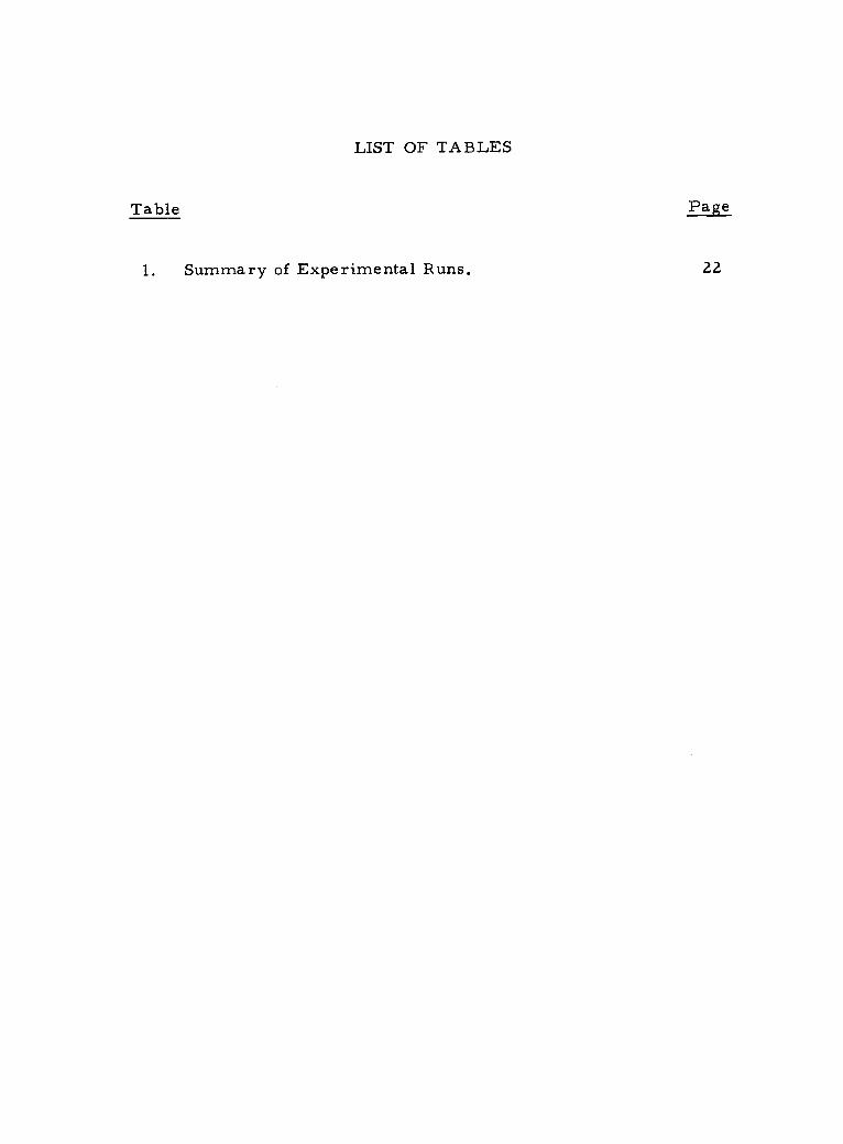
LIST OF TABLES
Table Page
1. Summary of Experimental Runs. 22
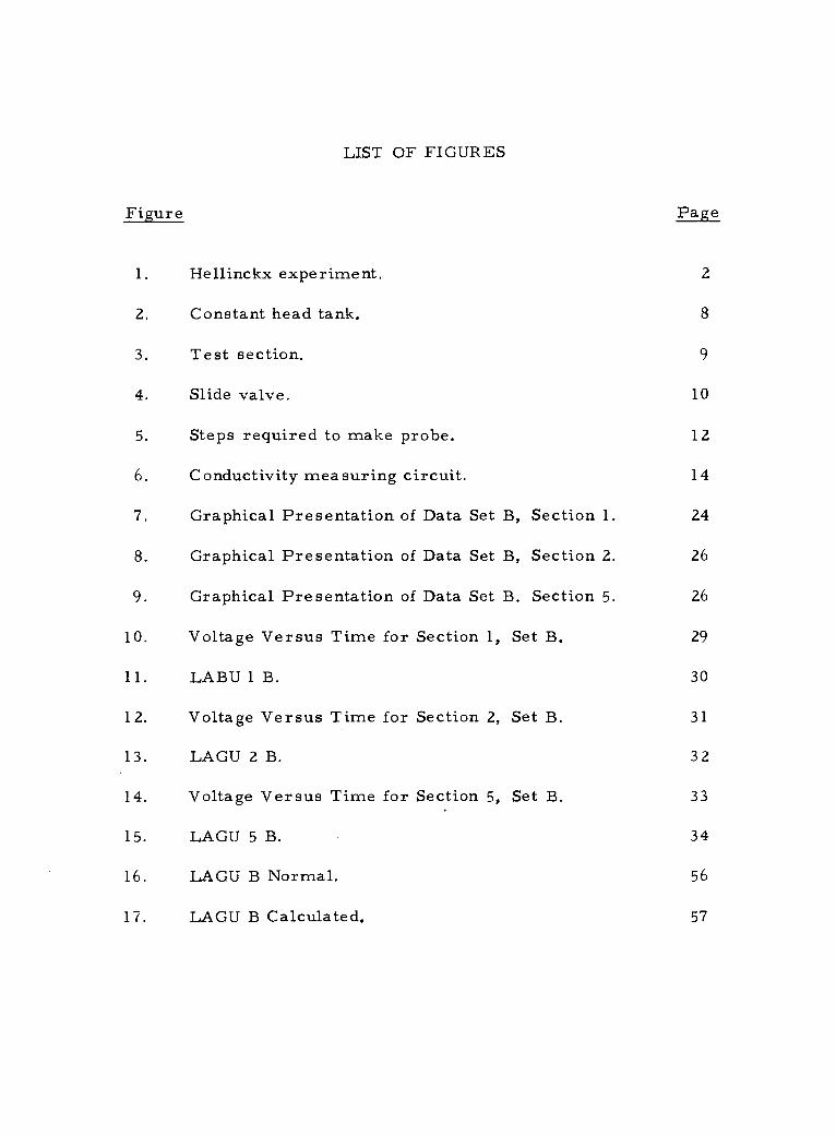
LIST OF FIGURES
Figure Page
1. Hellinckx experiment. 2
2. Constant head tank. 8
3. Test section. 9
4. Slide valve. 10
5. Steps required to make probe. 12
6. Conductivity measuring circuit. 14
7. Graphical Presentation of Data Set B, Section 1. 24
8. Graphical Presentation of Data Set B, Section 2. 26
9. Graphical Presentation of Data Set B. Section 5. 26
10. Voltage Versus Time for Section 1, Set B. 29
11. LABU 1 B. 30
12. Voltage Versus Time for Section 2, Set B. 31
13. LAGU 2 B. 3 2
14. Voltage Versus Time for Section 5, Set B. 33
15. LAGU 5 B. 34
16. LAGU B Normal. 56
17. LAGU B Calculated. 57
RESIDENCE TIME DISTRIBUTION IN TUBULAR FLOWVESSELS WITH MULTIPLE BAFFLES
INTRODUCTION
Plug flow is the flow for which all fluid elements have the
same residence time distribution and there is negligible diffusion
relative to the bulk flow. Fluid moves through the reactor with no
mixing of earlier and later entering fluid. In other words, there
is no backmixing of fluid elements of different ages.
Plug flow is desirable in most cases where chemical or nuclear
reactors are used. For most flow reactions where high conversion
and good product selectivity are needed, the optimal residence time
distribution, (RTD), is that of plug flow, where all molecules spend
the same amount of time in the vessel. Plug flow is also required
in true countercurrent mass transfer and heat transfer.
In most cases using tubular vessels, circular baffles are used
in order to prevent gross backmixing and to approach more closely
the condition of plug flow. The effect of these baffles on total
residence time distribution is not yet known. The main objective
of this project was to study the effectiveness of baffles for improving
the plug flow characteristics within tubular vessels.
L. J. Hellinckx et al. (1972) studied this problem for a flow
system made up of consecutive compartments. They assumed that
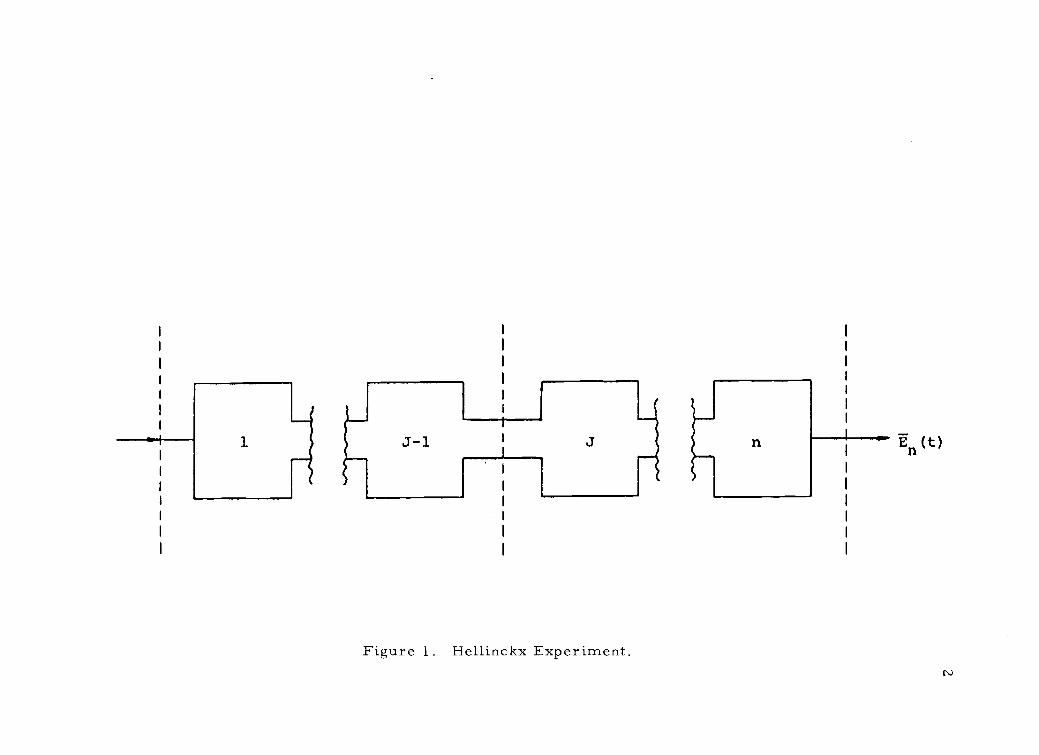
Figure 1. Hellinckx Experiment.
En (t)
N)

3
the consecutive flow regions of the systemwere independent.
They selected a flow system consisting of (n) successive flow
regions as shown in Figure 1. For each flow region they defined a
function G.(
t ) such that the E.(t), the overall age distribution function
in the effluent system j, is given as a function of the overallEj- 1
age distribution function in the effluent of system j-1, and of the
function G.(t).
where
E.( t ) = G.(e)E. (t-e)dec)
j j- 1
G. (e) = the age spectrum generating function.
This integral implies that G. and E. are independent; if they areJ- 1
not independent, then the best that can be done is as follows:
Suppose G* is the conditional probability that a molecule
remains in the last section an amount of time t - \, given that the
same molecule spent a total time X. in the first (j-1) sections;
accordingly,
i.(t) (X )G*(t-X , x )dX.J -1
Clearly G* (t-X ,X ) is a 2-place function depending on both (t-X )
and X and can be integrated over X but cannot be factored into the
product of two independent probability density functions as indicated
4
in Hellinckx article; therefore, Hellinckx approach does not appear
to be correct.
S. Veeraraghavan and P. L. Silveston (1971) studied the
influence of vessel dimensions and fluid velocity on resident time
distribution. They found that the length to diameter ratio, 1/D
exerts the major influence on the RTD. At 1/D< 2. 5, the RTD
resembles the response to a pulse signal of a well-stirred vessel
with bypassing. Both Reynolds Number, NRe, and nozzle to vessel
diameter ratio, d/D, effect the RTD. At 1/ D>5. 2, NRe and d/D
were found to have negligible affect on the RTD. In this experiment,
as will be explained in detail later, the first ratio used was
30 inches1/D - - 7. 50 ;4 inches
this is greater than 5. 2. The second ratio used was
15 inches1/D = - 3. 75 ;4 inches
this is between the two limiting ratio values of 2.6 and 5.2.
Suppose there are two vessels which are connected to each
other; further suppose it takes "t" seconds for a molecule of fluid
to go through these two vessels. If each molecule remains I
seconds in the first vessel it will stay in the second vessel (t-T)
seconds. The only case in which it can be said that the overall
residence time distribution is equal to the convolution of the RTD's

5
in each vessel is when the residence time distribution in one vessel
is independent of the RTD in the other. In this particular case:
where:
E1(T)
E2(t-T)
tEoverall (t) = f E
1(T)E
2(t-T)dT
0
= residence time distribution in the first vessel
= residence time distribution in the second vessel
Eoverall (t) = total residence time distribution.
Accordingly a series of n stirred tanks, each with an RTD of 1/T
exp (-t/T); has an overall RTD of (t/T)I1-1 exp (-t/T), which is the
n-fold convolution of 1/T exp (-t/T) with itself. But if the residence
time of a molecule in one vessel is dependent on its residence time
distribution in a preceding one, then the convolution will not work.
For example, in two adjacent sections of pipe through which the
fluid flows as laminar streamlines, it can be seen that for a length
of AL, the RTD will be
2AL 1 A2 (v-- ) 3 U
0(t-LV )
c t
for the total length of L, the RTD will be
L 12 (v ) 2 uo (t-c t
which is not the multiple convolution of
6
AL 2 1 AL2 (-) t 3 UO (t--
c-V )
c
In this project, as will be discussed in detail later, the residence
time distribution in each section will be found. It will then be
tested to see if the residence time distributions convolute to each
other.
7
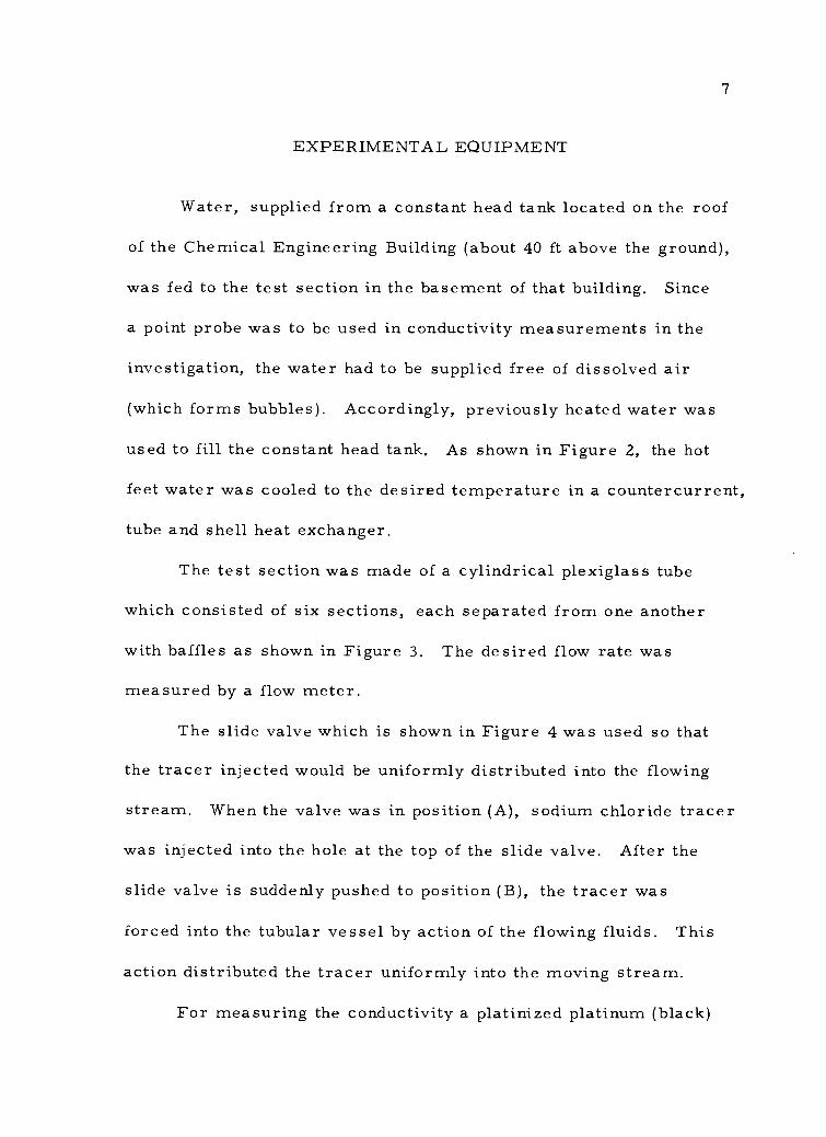
EXPERIMENTAL EQUIPMENT
Water, supplied from a constant head tank located on the roof
of the Chemical Engineering Building (about 40 ft above the ground),
was fed to the test section in the basement of that building. Since
a point probe was to be used in conductivity measurements in the
investigation, the water had to be supplied free of dissolved air
(which forms bubbles). Accordingly, previously heated water was
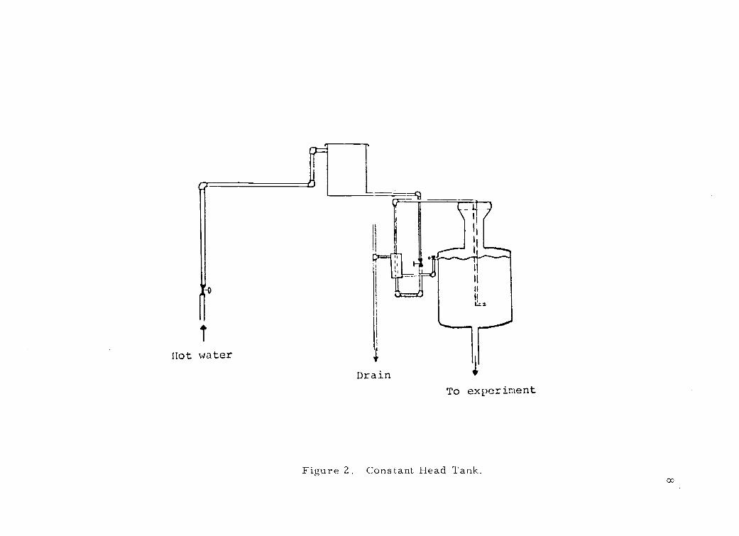
used to fill the constant head tank. As shown in Figure 2, the hot
feet water was cooled to the desired temperature in a countercurrent,
tube and shell heat exchanger.
The test section was made of a cylindrical plexiglass tube
which consisted of six sections, each separated from one another
with baffles as shown in Figure 3. The desired flow rate was
measured by a flow meter.
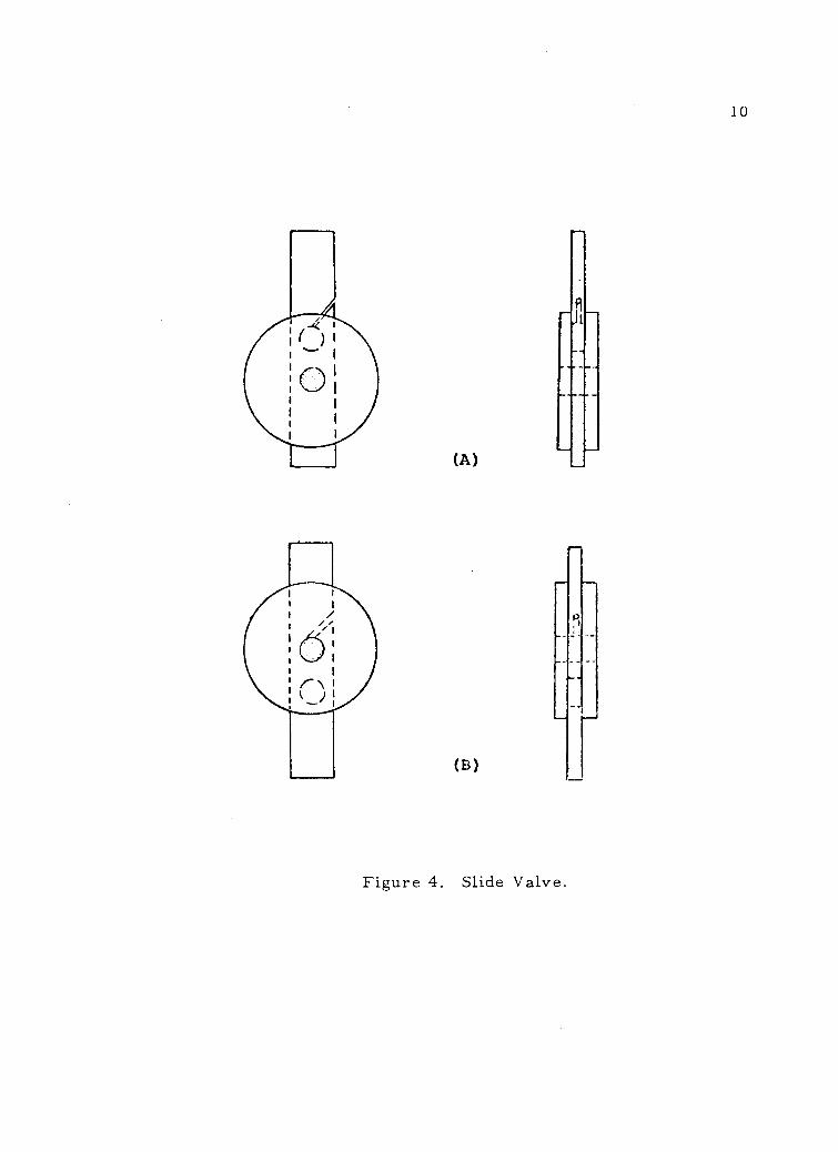
The slide valve which is shown in Figure 4 was used so that
the tracer injected would be uniformly distributed into the flowing
stream. When the valve was in position (A), sodium chloride tracer
was injected into the hole at the top of the slide valve. After the
slide valve is suddenly pushed to position (B), the tracer was
forced into the tubular vessel by action of the flowing fluids. This
action distributed the tracer uniformly into the moving stream.
For measuring the conductivity a platinized platinum (black)
Not water 4
Drain
I,
1
I
1
Lz.z
%......-. ---
To experiment
Figure 2. Constant Head Tank.CO

From constant head tank
Pro:Je connected to a conductivity monitoring circuit
Slide valve
Drain
Figure 3. Test Section.
(A)
(B)
r-
Figure 4. Slide Valve.
9JI
10
11
electrode was used. This method was introduced by Kohlrausch in
the late 1890's for the measurement of the conductivity of electrolytic
solutions (Geddes, 1972). Since Kohlrausch's time, the platinum-
black electrode has been used with gaseous hydrogen as the standard
reference electrode; it is still the most practical and accurate
electrode for electrolytic conductivity cells because the electrode-
electrolyte impedance is reduced to a very low value by the platini-
zation process. The method advocated by Kohlrausch is still used
to produce a platinum black deposit on platinum electrode. The
electrode is first cleaned thoroughly and placed in a solution of
0. 025N hydrochloric acid containing 3% platinum chloride and
0. 025% lead acetate. Failure to include the lead acetate results in
a stronger deposit having a velvety black appearance. A direct
current is passed through the solution via a large-area platinum
anode, and the electrode to be blackened is made the cathode. In
these cases both cathode and anode are made of platinum.
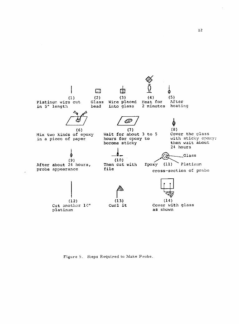
A twenty-thousandths inch diameter platinum wire which had
been cut into a five-inch length was used to make the conductivity
probe. The step-by-step production of the probe is illustrated in
Figure 5.
The conductivity probe used in this experiment measured
the potential difference when ions were transferred through the
water flowing in the tubular vessels. This voltage difference was
(1)
Platinum wire cutin 5" length
12
(2) (3) (4) (5)
Glass Wire placed Heat for Afterbead into glass 2 minutes heating
(6) (7)
Mix two kinds of epoxy Wait for about 3 to 5in a piece of paper hours for epoxy to
become sticky
(9)After about 24 hours,probe appearance
(12)Cut another 10"platinum
(10)Then cut withfile
(13)Curl it
(t)
(8)Cover the glasswith sticky epoxy;then wait about24 hours
Glass
Epoxy (11) Platinum
cross-section of probe
Figure 5. Steps Required to Make Probe.
(14)Cover with glassas shown
13
directly related to the concentration of sodium chloride tracer.
By using a point probe the conductivity can be measured at
a point. Since the surface area of a point electrode is much
smaller than that of a wire ring electrode, the current flow, and
thus the conductance through the probe, will be proportional to the
concentration near the point electrode (Khang, 1975). The fluid
conductivity near the coiled wire has very little effect on the cur-
rent flow while the conductance of the fluid close to the point elec-
trode will affect the current flow through the probe.
The putput signal from the amplifier, Number 1 in Figure 6,
was amplitude modulated with a carrier frequency given by the sine
wave signal generator. The carrier frequency was much higher
than the frequencies of the concentration signal. Since the output
signal picked up noises whose frequencies were higher and lower
than the carrier frequency, a band pass filter was used to block
frequencies which were much higher or much lower than the
carrier frequency.
Because a single diode produces an offset which is appreciable
when input voltage is small, an operational amplifier with two diodes
of the same characteristic was used as a precision rectifier.
The output signal still had high frequency components associ-
ated with the carrier frequency. By using a low pass filter the
high frequency components were removed without adding a
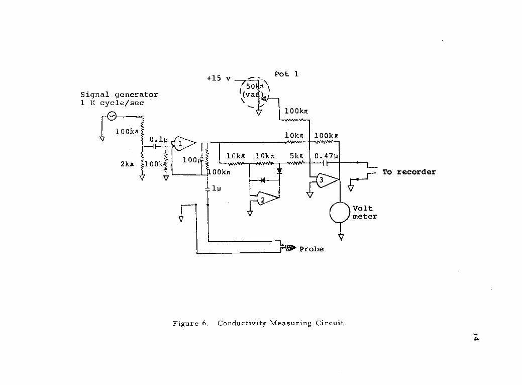
Signal generator1 K cycle /sec
100kni0.1p
2kx 100k }
+15 v
100
50 ft
(va
Pot 1
100kn
10ki 100kx
1Ckn 10kg 510t 0.47p
Probe
s*
0 Voltmeter
V
Figure 6. Conductivity Measuring Circuit.
To recorder
15
significant time constant to the system. In this experiment the sig-
nal generator has an amplitude of 2 volts and a frequency 1 of KHz.
16
THEORY OF CALCULATIONS
The conductivity was measured at three different points after
the first, second, and fifth sections. This permitted the evaluation
of the residence time distribution functions after the first, second,
and fifth sections.
After finding the tracer output, plots were obtained (for which
the equations were unknown to the experimenter). Since there were
noises on the curves, it was decided to smooth each of the curves
by using Laguerre polynomial.
Approximate each impulse response curve, F(t), by
F(t) = A L +A L +A L +A L +.A L +A L0 0 1 1 2 2 3 3 4 4 5 5
where L0, L1, L2, L3, L4, L5. . . are orthonormal. For finding
AO both sides of this equation were multiplied by L0.
L0F(t) = A
0 0L2+A
1LOLL +A
2L
0L
2+A
3L
0L3 +. .
By taking an indefinite integral of both sides of the equation, one
obtains
CO OD CO
r- L0F(t)dt = f A
0 0L 2dt
+ f A1LOL1 dt + f A2L0
L2dt
+ . .
0 0 0 0
The property of orthonormality reduces this equation to
co
L0
F(t)dt = A00
By the same method, A1, A2, . . An can be determined.
co
A0
= f L0(t)F(t)dt
0
Al = LI (t)F(t)dtf0
co
A2 = f L2(t)F(t)dt
0
co
A3 = r L3(t)F(t)dt
0
co
A4 = r L4(t)F(t)dt
0
co
A5 = L5(t)F(t)dt
0
According to Solodovnikov (1960), each of the time dependent
Laguerre functions can be expressed by:
v-k+1/2/2tv 2v-1/2 v-12v tLy(t) = e-t 2v+1
+. . . +v! (v-1)!
v! (-1)k
k![(v-k)!] 2tv-k -+ . . . + 21/2 (-1)vl
17
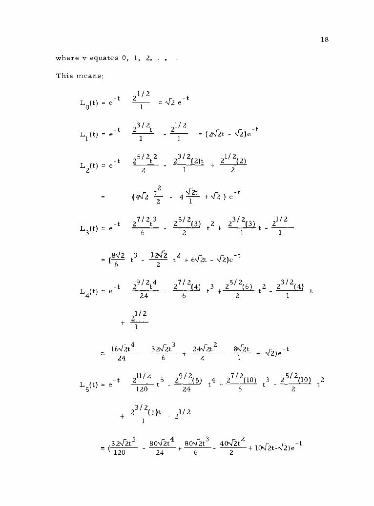
18
where v equates 0, 1, 2. .
This means:
1/2L
0(t) = e-t
14-2 e-t
1/2Ll(t) e-t 2
1
3/2t 2
1- (2\r2t t
23/2
(_2)t 21/2(2)2
L (t) = e-t 25/2t22 1 2
t2(4v2 2 44-2t
+ ) et
1
7/2 3 25/2(3) t2 23/2(3) 21/2L
3(t) = e-t 2
6
t2 1 6 1
r= (r2 t 3 122 t2 + 6\r2t N2)e
-t6 2
9/242 (4)7/2
3 25/2(6) 2 23/2(4)L
4(t) e-t 2
24t
6t + t
21/21
r 4 r 3 .1-16N/2t 3 2NI 2f 24N 2f 8Nr2t .r -t
+ Ni 2)e24 6 2 1
-t 211/2 5 29/2(5j t+4 27/2(10) t3 25/2(10) taL (t) = e
5 120 24 6 2
23/2(5)t- 21/2
1
324-2t5 804-2t4 80\r2t3 40,4-2t2 -t10Nr2t-N 2)e
120 24 6 2
By knowing F(t) data from the experiment and knowing L1,
L2, L3, . . Laguerre polynomial coefficients can be obtained by
numerical integration. This provides all of the terms of the
Laguerre polynomial:
F(t) = A0
L0
+A1L
1+A
2L2+ .
Accordingly, the Laguerre polynomial approximation can be
obtained for each of the three measured sections of the test tubular
vessel.
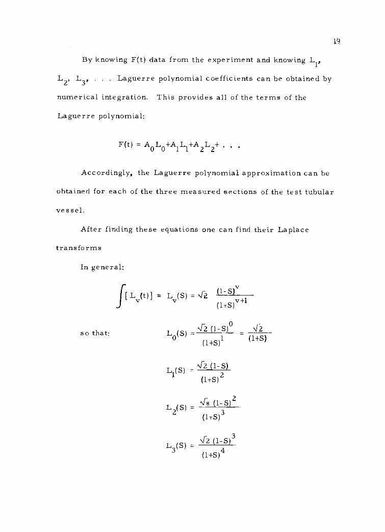
After finding these equations one can find their Laplace
transforms
In general:
so that:
Lv(t), = Lv(s) = 42 (1- S)v
L (S) 4-2 (1-S)° 4-20
(1+S)1(1+S)
(S) - T2 (1-S)L1
(1+S)2
4-s (1-S)2L 2(S) - 3(1+S)
L3(S)
4-2 (1-S)3
(1+S)4
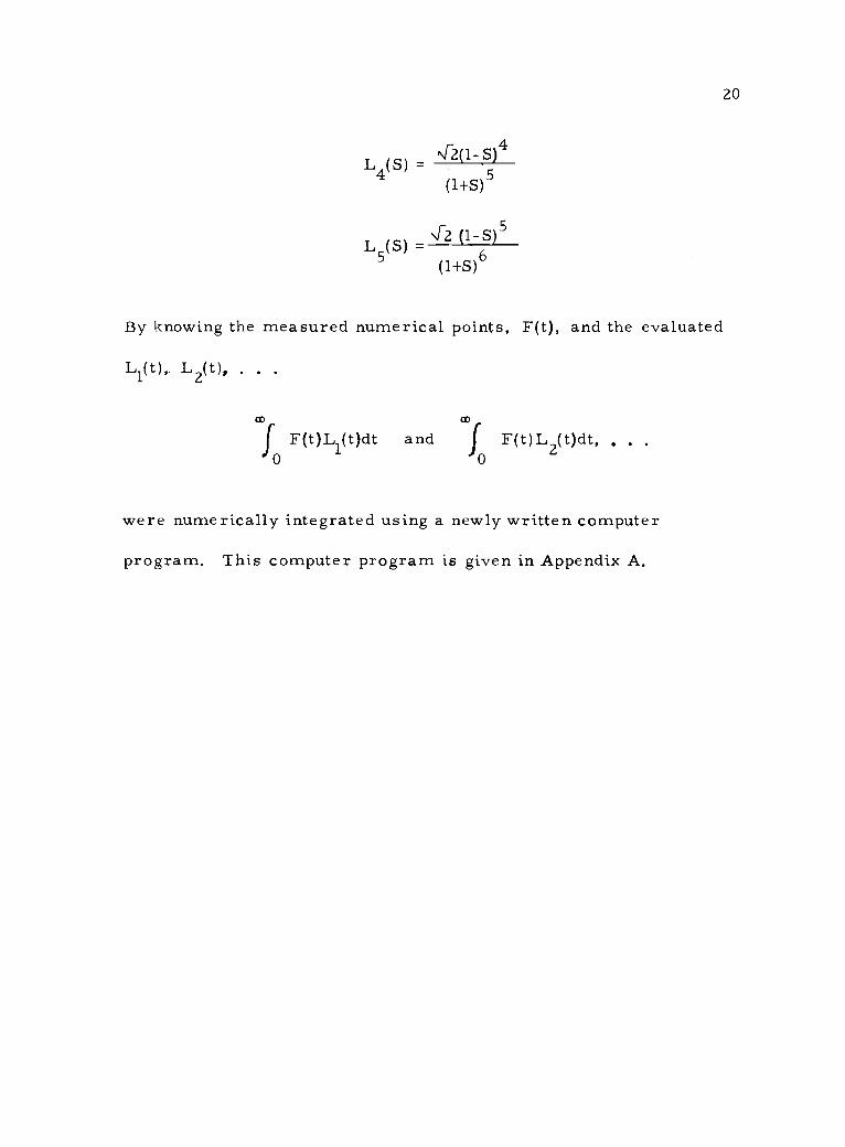
20
L4(S) -[2(l S)4
5(1+S)
4-2 (1-S)5L 5(S) -(1+S)
6
By knowing the measured numerical points, F(t), and the evaluated
L (t), L2(t), .
co co
F(t)Li(t)dt and f F(t)L2(t)dt,0 0
were numerically integrated using a newly written computer
program. This computer program is given in Appendix A.
21
ANALYZING THE DATA
Water from the constant-head tank was introduced into the test
section at a predetermined flow rate. After the system had reached
steady state, a tracer containing 15 grams of NaC1 per 200 cubic
centimeters of water was injected into the hole provided in the slide
valve. This tracer was instantaneously distributed uniformly into
the flowing water stream by pushing the slide valve into its second
position. By use of the probe which was installed inside the pipe,
the conductivity of the water was measured and recorded on a
plotter as a plot of the potential difference, v, versus the time, t.
Digitizing produced a set of numbers (almost 50 points per
inch). By using the Laguerre function, the curve was smoothed;
this resulted in a set of graphs as shown in Figures 10 through 15.
To find the convolution integral of two of these graphs the Laplace
transform of each graph was taken and then multiplied by the
transform of the other graph.
Twelve sets of data were experimentally measured to include
two different lengths of individualized sections, two different orifice
diameter to tube diameter ratio and three different flow rates.
Table 1. summarizes the experimental parameters for each
set of data.
In the digitizing, 50 points per inch were read and the data
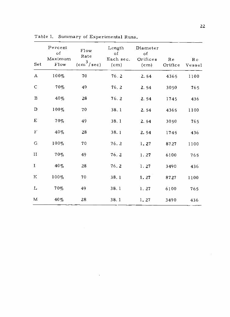
22
Table 1. Summary of Experimental Runs.
Set
Percentof
MaximumFlow
FlowRate
(cm3/sec)
Lengthof
Each sec.(cm)
Diameterof
Orifices(cm)
ReOrifice
ReVessel
A 100% 70 76. 2 2.54 4365 1100
C 70% 49 76. 2 2. 54 3050 765
B 40% 28 76. 2 2. 54 1745 436
D 100% 70 38. 1 2.54 4365 1100
E 70% 49 38. 1 2. 54 3050 765
F 40% 28 38. 1 2. 54 1745 436
G 100% 70 76. 2 1. 27 87 27 1100
H 70% 49 76. 2 1. 27 6100 765
I 40% 28 76. 2 1. 27 3490 436
K 100% 70 38. 1 1.27 8727 1100
L 70% 49 38. 1 1. 27 6100 765
M 40% 28 38. 1 1. 27 3490 436

23
points were stored (for example, set B was stored in *CHEMB).
Then by using computer programs "LISTER" and "EDITOR",
"GRAPH 1B" (data points for Section 1, set B), "GRAPH 2B"
(data points for Section 2, Set B) and "GRAPH 5B" (data points for
Section 5, Set B) were obtained. Program "LISTER" put a counter
for each number. Program "EDITOR" separated the data for each
section and put the data for each section in a special file. Both
computer programs are given in Appendix A.
To illustrate the calculations, consider Set B:
Set B: pipe diameter 10. 16 cm = 4 inches
Section 1 baffle orifice diameter 2. 54 cm = 1 inch
length of each section 76. 2 cm = 30 inches
40% flow rate
v = 40% flow rate = 28 cubic centimeters/sec
V = volume of each section = (Tr D 2 /4)L
V =3.144 1593 (42) 30 = 3.769911 x 102 inch3
or V = (3. 769911 x 102) (2. 54)3 = 6178 cm 3
V 6178 220.64 secv 28
N for V equal to 220. 64 = 551, where N is the
equivalent digitized number
24
0 =N Nh
N- NV h
M = N- Nh
0 216 5510
2461 N
86.40 220.64 984. 4
0 1 6.7015>- 8
0 335 2245
Figure 7. Graphical Presentation of Data Set B, Section
If h1
is used to designate the dead time, or time after the tracer
-7` M
is first introduced before the first voltage response, the plot
indicates:
hl = 86.40 sec
Nh = 216 digitized points1
t =V= time of backmixing - v hl
t = 220. 64-86. 40 = 134. 24 sec
N for t = 335 digitized points
25
With this information a computer program "SATVAT", was used
to obtain A0, A1, , A5 for the Laguerre function. Pro-
gram "SATVAT" involved a trapezoidal rule which calculated
A0
=
co cc
fF(t)L0 (t)dt, Al = F(t)L1(t)dt,0
co
A5 f F(t)L5(t)dt0
This computer program is located in Appendix A with the other
programs used in this study.
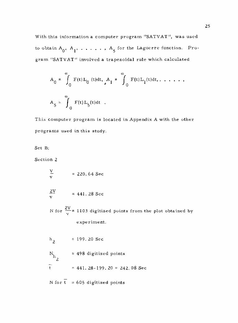
Set B:
Section 2
V
2V
= 220. 64 Sec
= 441.28 Sec
N for 2Vv = 1103 digitized points from the plot obtained by
experiment.
h2
= 199. 20 Sec
Nh = 498 digitized points2
t = 441. 28-199. 20 = 242. 08 Sec
N for t = 605 digitized points
0
Figure
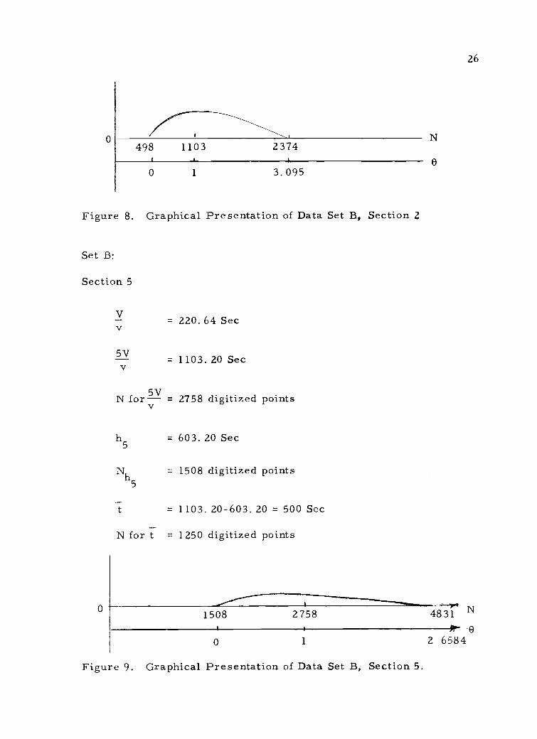
Set B:
Section
0
26
N498 1103 2374
0
8. Graphical
5
V
5V
1 3. 095
Presentation of Data Set B, Section 2
= 220.64 Sec
= 1103. 20 Sec
-- 2758 digitized points
= 603. 20 Sec
= 1508 digitized points
= 1103.20-603.20 = 500 Sec
= 1250 digitized points
N for
h5
Nh5
t
N for t
1508 2758 483T N*-
0 1 2e
6584
Figure 9. Graphical Presentation of Data Set B, Section 5.
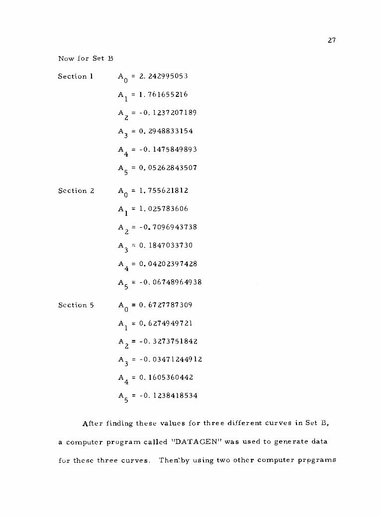
Now for Set B
Section 1
Section 2
Section 5
A0 = 2.242995053
Al = 1.761655216
A2 = -0.1237207189
A3 = 0.2948833154
A4 = -0.1475849893
A5 = 0.05262843507
A0 = 1.755621812
Al = 1.025783606
A2 = -0.7096943738
A3 = 0.1847033730
A4 = 0.04202397428
A5 = -0.06748964938
A0
= 0.6727787309
Al = 0.6274949721
A2 = -0.3273751842
A3 = -0.03471244912
A4 = 0.1605360442
A5 = -0.1238418534
27
After finding these values for three different curves in Set B,
a computer program called "DATAGEN" was used to generate data
for these three curves. Then lby using two other computer prpgrams

28
called "PLOT" and "PLOTTER", *GRAPH 1B and LAGU 1B (which
is its equivalent Laguerre function) were plotted. The same process
was repeated for *GRAPH 2B, LAGU 2B and *GRAPH 5B, LAGU 5B.
The computer programs are in Appendix A.
Before convoluting the curves, each curve must be normalized.
This required that
co
fF(t)dt0
be equal to one.
For graph 1B each of the coefficients were divided by
5.771202340 which was the value of
co
fF(t)dt0
when using the old coefficients. This normalized the curve and
produced a new set of coefficients:
A0
= 2.242995053/5.771202340 = 0.3886529913
Al = 1.761655216/5.771202340 = 0.3052492552
A2 = -0.1237207189/5.771202340 = -0.02143759855
A3 = 0.2948833154/5.771202340 = 0.05109564663
A4 = -0.1475849893/5.771202340 = -0.02557265897
A5 = 0.5262843507/5.771202340 = 0.00911914570

L J(,-1 1 I I 1:7 (7 5 E El N N 371 37i [C. f'
NI Cl L IC El I Cl G El ClI_ LI1 L:71
L U L J L j J L
Figure 10. Voltage Versus Time for Section 1, Set B.
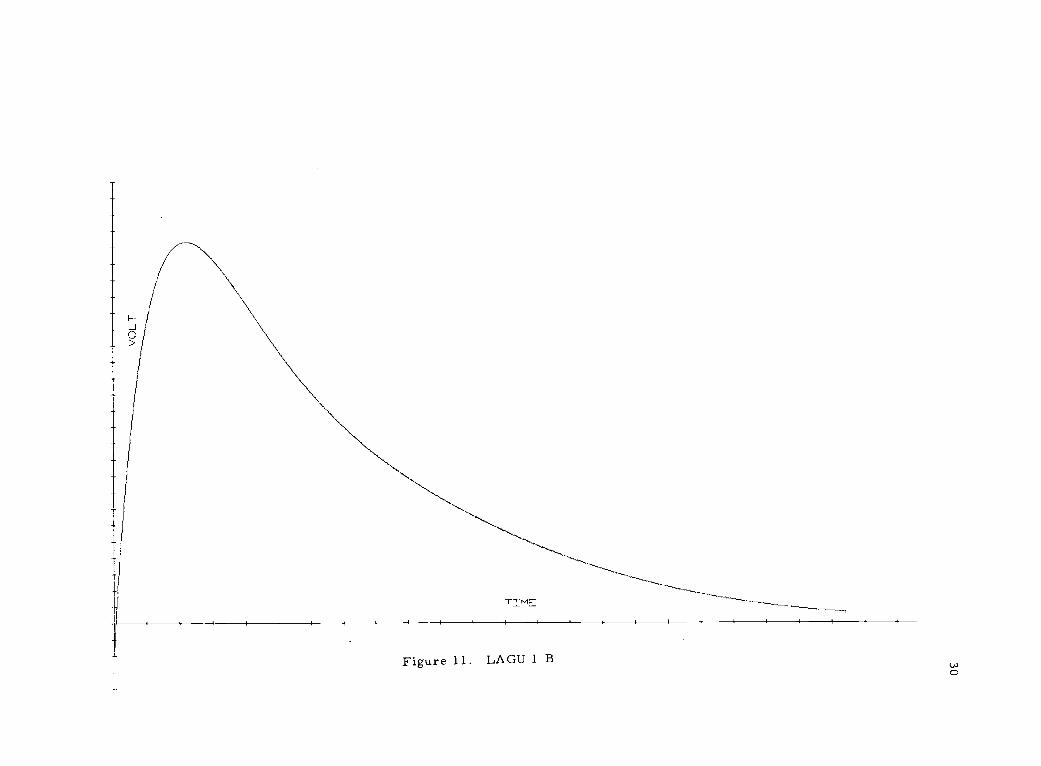
Figure 11. LAGU 1 B

t
FJ
0 Fs Fs 1\i;
1\:) [Ti Liri
1\-_J 1.4 W I I VI Lrl CF; i Oi JJ CC Iil LilM Li 1 0 D 1 [Ti N Ell U I 'J [Ti Li
[1 Ll [1 Li 113 U D Li Li Li Li LJ LJ D 1.1 D Li Li
Figure 12. Voltage Versus Time for Section 2, Set B.
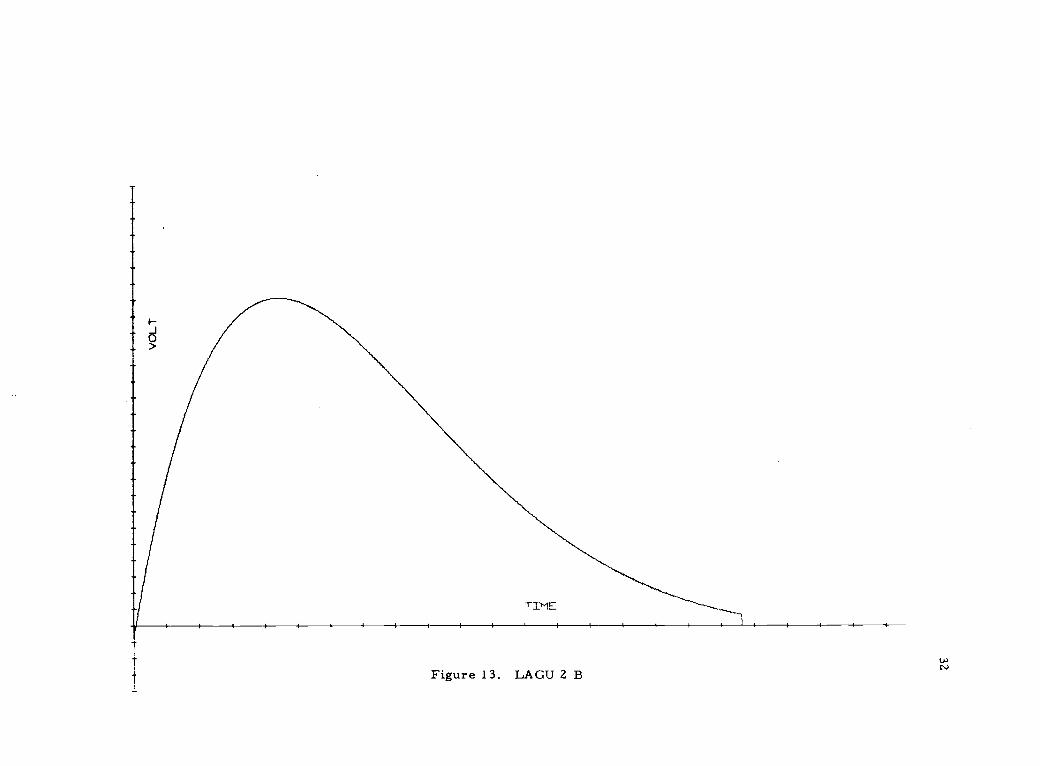
Figure 13. LAGU 2 B
T
1 CD F' F' 10 10 10 LA LA 1 1 1 MMEIVk) M ,11 N) CFI 1 3) M 1 M 10
LI
1 1 1 t-1111 11111 1111 11
\I M0]
01
CD W Li310
1' P.
1P.
03
I"
100
I"F'M
I" P.10ILi
I"100
I"L
100
I" I" I" P. I" V' I"LA 1 1 I in in Cr M0] I Co to ori r. 1
L.1
M Vt.-)
V0
P.3] 0
131113
F'Wto
F'LO
(T)
tJ
Figure 14. Voltage Versus Time for Section 5, Set B.

0_>
4111f111111-L
11114141111111111
Figure 15. LAGU 5 B
IIIIIIIII
35
The Laguerre function with these coefficients can then be
normalized.
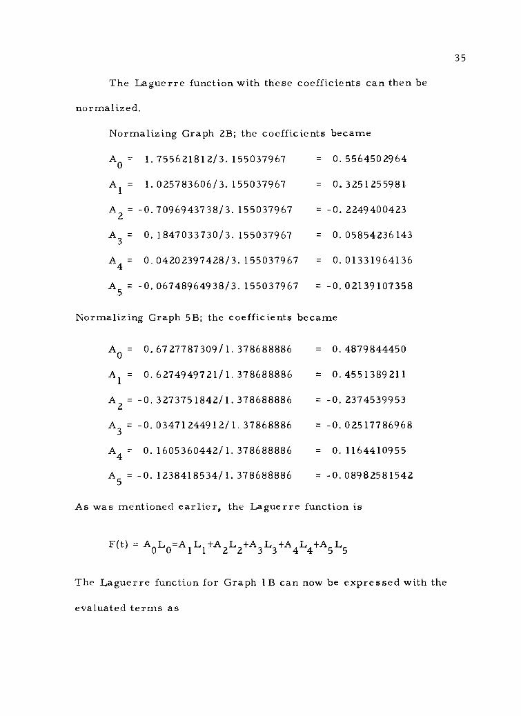
Normalizing Graph 2B; the coefficients became
A0
= 1. 755621812/3. 155037967 = 0. 5564502964
Al = 1. 025783606/3. 155037967 = 0.3251255981
A2 = -0.7096943738/3. 155037967 = -0. 2249400423
A3 = O. 1847033730/3. 155037967 = 0.05854236143
A4 = O. 04202397428/3. 155037967 = O. 01331964136
A5 = -0.06748964938/3. 155037967 = 0.02139107358
Normalizing Graph 5B; the coefficients became
A0
= O. 6727787309/1. 378688886 = 0.4879844450
Al = O. 6274949721/1. 378688886 = 0.4551389211
A2 = -0. 3273751842/1. 378688886 = -0. 2374539953
A3 = -0. 03471244912/1. 37868886 = -O. 02517786968
A4 = O. 1605360442/1. 378688886 = 0, 1164410955
A5 = -0. 1238418534/1. 378688886 = - 0.08982581542
As was mentioned earlier, the Laguerre function is
F(t) = A L =A L +A L +A L +A L +A L0 0 1 1 2 2 3 3 4 4 5 5
The Laguerre function for Graph 1B can now be expressed with the
evaluated terms as
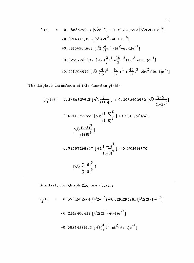
f1(t) =
36
r0. 3886529913 [ '[2e -t ] + 0. 305249552 [Nr2(2t-l)e -t
- 0. 02143759855 [4-2,(2t2-4t+l)e-t]
+0. 05109564663 [ (1t3
0. 02557265897 [4-2 (3t4
+0. 0911914570 [4-2 t5 -
-6t 2+6t-1)e -t]
16 3 2--3- t +12t -8t+1)e-t]
10 40 3 2t4 + t -20t +10t-fle -t
3 3
The Laplace transform of this function yields
r r (1-S{f1(t)}= 0. 3886529913 [v2 ](1+S)
+ 0. 3052492552 [V22]
(1+S)
c12-0. 02143759855 ] +0. 05109564663[4-2
(1+S)
[4-2(1-5)3
(1+5)4
4-0. (1-S)5 + 0.091191457002557265897 [4-2
(1+S)
(1+5)6
Similarly for Graph 2B, one obtains
rf2(t) = 0. 5564502964 [v2e -t ] +0. 3251255981 [4-2(2t-l)et]
-0. 2249400423 [42(2t -4t+l)e-t]
r 4 3 2+0. 05854236143 [V2(-3 t -6t +6t-l)e -t
37
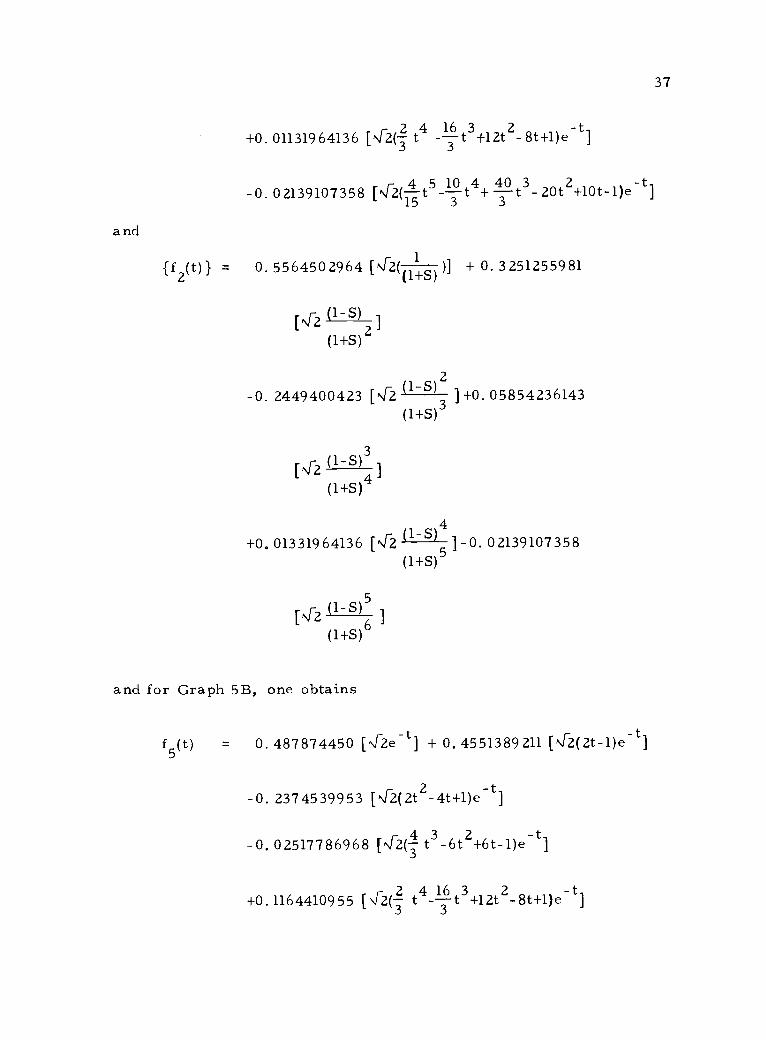
+0.
-0.
and
{f2(t)} = 0.
2 1601131964136 [
rN./2(.-i t
4---3-t
02139107358 [4-2(-1-t5_10
15
3+12t
t4+
+ 0.
2-8t+l)e -t]
40 3_t 20t2+10t-1)e-t]3
32512559815564502964 [4-2((1 )]
(1 -S)
(1+s)
2
-0. 1 +0. 058542361432449400423 [4-2 ]
(1 +S)3
(1-S)3
(1+S)4
+0. P--S)4
-0. 0213910735801331964136 [42 ](1 +S)
and for Graph 5B, one obtains
f5(t) = 0. 487874450 [4-2e t] + O. 4551389211 [4-2(2t-1)e t]
-0. 2374539953 [Nr2(2t2
-4t+1)e-t
r 4-0. 02517786968 [\12(3 t3 -6t 2+6t-l)e -tI
16+0.1164410955 [\/r 2(-
2t4--
3t
3+12t
2 -8t+l)e-t]
38
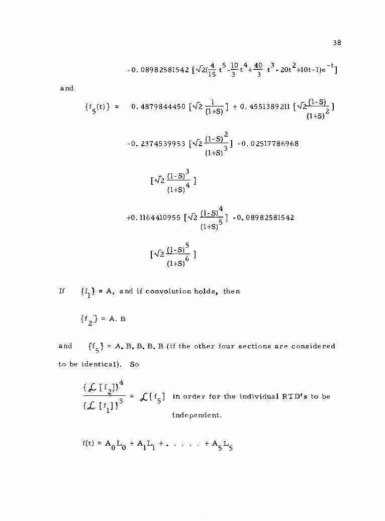
and
{f5(t) } =
-0.
0.
-0.
0 3_08982581542 [4-2(il t5 -3 tit4 20t2+10t-1)e-t]t
(14879844450 [42(1+S)
+ 0. 4551389 211 [N ]
(1+S)
c122374539953 [4-2 ] -0.02517786968
(1+S)
(1-5)3
(1+S)4
4+0.1164410955 14-2 1.---l-S)5 "I -0. 08982581542
(1+S)
5 ,
(1+S)6
If {f1} = A, and if convolution holds, then
= A. B
and {f5} = A. B. B. B. B (if the other four sections are considered
to be identical). So
= dC [ f5] in order for the individual RTD's to be
independent.
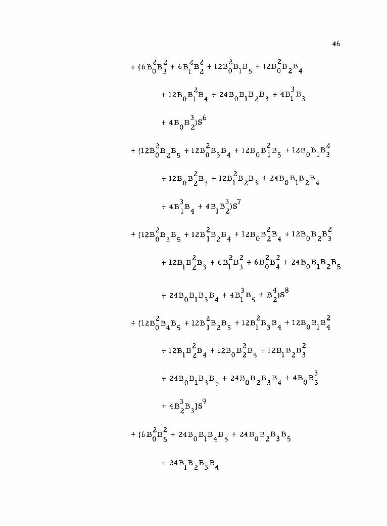
f(t) = AoLo + A1L1 + + A5
L5
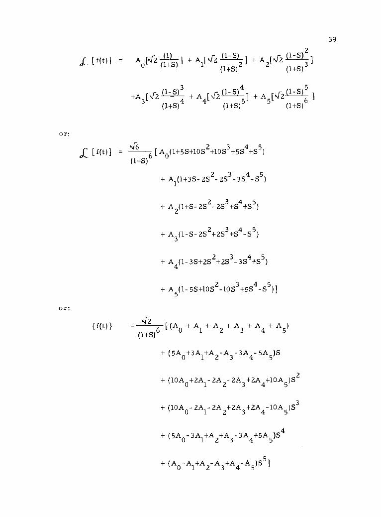
or:
or:
2
Jc [f(t)] = A [Nr2 (1) ]r,r, (1-S) + A [Nr2 (1-S) ]
0 (1+S ) 2(1+S)
2(1+S)
3
+A 31N-2(1 -S)3
+ A 4[ 42(1-S) + A 5r 42 (1-S)6
1
(1+S) (1+S) (1+S)
4-60C [ f(t)] _ [A0(1+5S+10S2+10S3+5S4+S5)(1+S)
{ f (t )}
+ A1(1+3S- 2S
2- 2S
3 -3S4-S5)
+ A2
(1+S- 2S2-
2S3+S 4
+S5)
+ A3(1 -S- 2S2+2S3
+S4- S5 )
+ A4
(1- 3S+2S2
+2S3
- 3S4
+S5)
+ A5(1 -5S+1052 -1053 +554 -S5)]
4-2 [ (A0 + Al + A2 + A3 + A4 + A5)(1+S)
+ ( 5A0 +3A1 +A 2- A3 3A4- 5A5)S
+ (10A0
+2A1-
2A 2- 2A3+2A
4+10A
5)S2
+ (10A 0- 2A1-
2A2+2A
3+2A
4-10A
5)S3
+ (5A 0-3A1+A
2+A
3-3A 4+5A 5)S4
+ (A0-A 1+A 2-A3
+A4-A5 )S5]
39
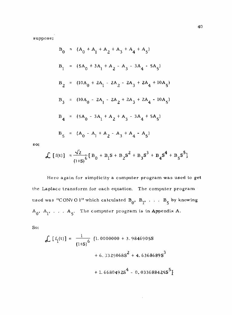
suppose:
B0 =
B1 =
B2 =
B3 =
B4 =
B5 =
so:
(A0 + + A2 + A3 + A4 + A5)
(5A0 + 3A1 + A2 A3 3A4 - 5A5)
(10A0 + 2A1 - 2A2 2A3 + 2A4 + 10A5)
(10A0 - 2A1 2A2 + 2A3 + 2A4 - 10A5)
(5A0 3A1 + A2 + A3 3A4 + 5A5)
(A0 Al + A2 - A3 + A4 A5)
dl.. [f(O] 4-2 [ B0 + B1S + B2S2 + B353 + B4
S4 + B 555](1+S)
40
Here again for simplicity a computer program was used to get
the Laplace transform for each equation. The computer program
used was "C ONV 0 1" which calculated B0, B1, . . . B5 by knowing
A0, Al, . . A5. The computer program is in Appendix A.
So:
L{yo] 1 {1. 0000000 + 3. 9846905S(1+S)
+ 6. 3325068S2 + 4. 636868953
+ 1. 6680492S4
O. 033688425S5}

[f 20] - 1 {1. 0000000 + 5. 0079315S(1+S)
6
+ 8. 9947915S 2+ 8. 0917999S3
+ 2.1122166S4 0. 024673770551
[ f5(t)] 1
{1. 0000000 + 5.2225050S(1+S)6
+ 7. 9903209S2 + 7. 8138965S3
+ O. 018980490S4 + 0. 037952272S 5}
Now what will be for, [f(O] }2?
[f(0] 122,,F-21
- " '1 [ BO + B1S
+ B2S2 + B3
S3 + B4
+ B S5]2
(1+S)
(4-2) 26) [ BO
2 + 2B OBIS + (2B0
B2 1
+ B 2)S2
(1+S)
+ (2BOB3
+ 2B1B
2)S3
+ (2B0B4 + 2B1B
3+ B 2)S4
+ (2BOB5
+ 2B1B
4+ 2B2B3)S5
+ (2B1
B5
+ 2B2
B4 3
+ B 2)S6
+ (2B2
B5 + 2B3
B4
)S7
+(2B3
B5 4
+ B2)S8 + 2B4
B5
S9 + B5
S10]
41
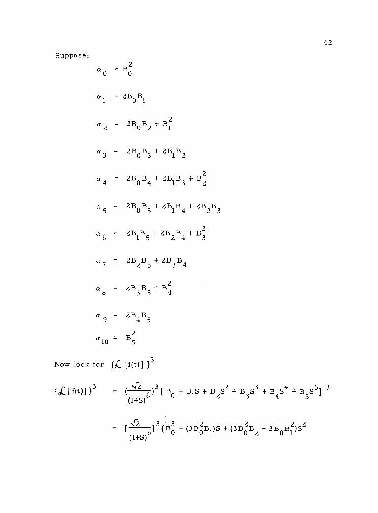
Suppose:
42
a = B0 0
= 2B Ba1 0 1
2
a = 2B B + B22 0 2 1
a3
= 2BOB3
+ 2B1B2
a4
= 2BOB4
+ 2B1 B3 + B23 2
a5
= 2BOB5
+ 2B1B4 + 2B
2B3
a6
= 2B1B5 + 2B
2B
4+ B2
3
a7 = 2B2B5 + 2B
3B4
a8 = 2B B + B23 5 4
= 2B4
B5
2
a10 = B5
Now look for
{0C[f(t)] }3
{k[f(t)] }3
4 2)
3B
0+B1 S+B
2S2+B
3S3 +B
4S4 +B 555]
3
(1+S)6
['f2 ]3
(1+S)-6 + (3B
0
2B
1)S+ (3B O2 B2 + 3B
OB12
)S2
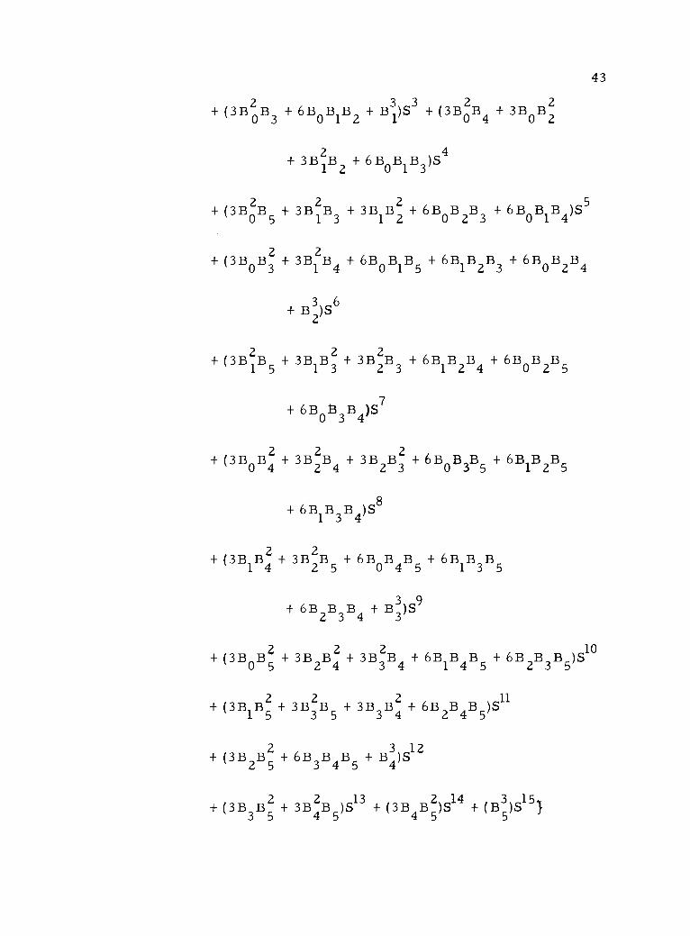
43
+ (3B0
B3
+ 6B0
B1
B2 + B 13 )S3
+ (3B O2 B4 + 3BOB2
2
+ 3B 2B2
+ 6B0
B1B
3)S4
+ (3B 2B5
+ 3B1
2B3 + 3B
1B2
2+ 6B
0B
2B3 + 6B
0B
1B
4)S5
0
+ (3B0 3
2B + 3B
1
2B4 + 6B0
BIB5 + 6B1
B2
B3 + 6B0
B2
B4
+ B 3
2)S6
+ (3B 2B5
+ 3B1 3B2
2+ 3B 2B
3+ 6B
1B
2B4 + 6B
0B
2B5
1
+ 6B0
133
B4
)S7
+ (3BOB4
2 + 3B B4 + 3B2
B32
+ 6B0
B3B5 + 6B
1B
2B5
+ 6B1B
3B
4)S8
+ (3B1B2 + 3B 2B
5+ 6B
0B
4B5 + 6B
1B
3B5
4 2
+ 6B2
B3
B4 + B 33 )S9
+ (3B0 5
B2 + 3B
2B4
2 + 3B3
2B4 + 6B1
B4
B5 + 6B2B3B5)S10
+ (3B1B5
2 + 3B 2B5
+ 3B3 4
B2 + 6B2
B4
B5
)S11
3+ (3B2B5
2 + 6B B4 B + B4
)S12
3 4 5
+ (3B3 5
B24
+ 3B 2B5
)S13 + (3B4
B2
)S14 + (B5
3)S
15}

suppose:
{ f (t ) 1 } 3
44
Nrz- [ ]3 {C0 + CiS + C
2S2 +
(1+S)
where
Co =
C1 =
C2 =
C3 =
C4 =
C5 =
C6 =
+ C14
S14 + C15
S15}
BO3
3B O2 B1
3B 2B2
+ 3B B20 0 1
3B02 B3 + 6B
0B
1B2 + B1
3
3BOB4
+ 3B0 2 1
B2 + 3B 1B2 + 6B0
B1
B3
23B O2 B5 + 3B
2B3
+ 3B1B2 6B
0B
2B
3+ 6B
0B
1B4
3BOB3
2 + 3B1
2 B4 + 6B 0BIB5 + 6B1B
2B3 + 6B
0B
2B4
+ B32
C7 = 3B2B
5+ 3B
1B3
2
2+ 3B 2B
3+ 6B
1B
2B4 + 6B
0B
2B5
1
+ 6B0
B3
B4
2C8 = 3B
OB4+ 3B
2
2 B4 + 3B2
B32 + 6B
0B
3B5 + 6B
1B
2B5
+ 6B1B
3B4

45
C9
= 3B1B2 + 3B 22
B5
+ 6B0
B4
B5 + 6B1B
3B5 + 6B
2B
3B4
+ B33
C10 = 3B0
B2 + 3B2 4 3B2 + 3B 2B
4+ 6B
1B
4B5 + 6B2B3B5
C11 = 3B1
B2 + 3B 2B5
+ 3B3 4
B2 + 6 B2B4B55 3
3C12 = 3B
2
2B + 6B
3B
4B5 + B4
5
2C13 = 3B3 B5B + 3B4
B52
C14 = 3B B24 5
3C15 = B5
Now look for [f(O] 14
{ [f(t)] }4 = [ ]4{130 + B1S + B
2S2 + B
3S3 B
4S4 + B
5S5} 4
(1+S)
= Bo4 + (4B 3B )S + (4B 3B + 6B
0
2B
1
2)S2
0 0 2
+ (4BOB3
+ 12B2
B1B
2+ 4B
0 1B
3)S3
0
3+ (4BOB4
+ 12B0
B1B3 + 12B
oB
2B2
+ 6B 2B + B
4)S4
1
22
+ (4B3B+ 12B
OB1
2B3 + 12B0
B1B
4 0+ 12B 2 B B
5 2
2 3+ 12B
0B
1B2 + 4B
1 B 2)55
46
+ (6B O2 B32 + 6B 2
B2 + 12B0
B1B
5 0
2+ 12B B B2 2 4
+ 12BOB1
2B4 + 24B0
B1B
2B3 + 4B
1
3B3
+ 4B0
B2)S
6
+ (12B2
B2
B5
+ 12B2
B3
B4
+ 12B0
B12 B5 + 12B
0B
1B3
2
+ 12B0
22
B B3
+ 12B2
B2
B3
+ 24B0
B1B
2B4
3+ 4B 3B + 4B
1B
2)S7
1
+ (12B 2 B B + 12B1B B4 + 12B
0 2B
2B4
+ 12B0
B B23 5
22 3
2+ 12B
1
22
B B3 1 3
2+ 6B 2B + 6B O2 B4 + 24B
0B
1B
2B5
+ 24B0
B1B
3B4 + 4B 3B
5 2+ B4
)S8
+ (12B02
B4
B5 + 12B2 B B + 12B
1
2B
3B4 + 12B
0B
1B4
21 2 5
+ 12B B2B + 12B B 2B + 12B B B21 4 0 2 1 2 3
3+ 24B
0B
1B
3B5 + 24B
0B
2B
3B4 + 4B
OB3
+ 4B3B3
)S9
+ (6B O2 B52 + 24B
0B
1B
4B5 + 24B
0B
2B
3B5
+ 24B1B
2B
3B4
47
+ 12B2 B B + 12B
0B B2 + 12B
1B
22 B5 + 12B
0 3B
2B1 3 5 2 4
+ 6B2
B21 4
3+ 6B 2
B2 + 4B B3 + 4B2
B4)S
10
2 3 1
+ (12B0
B1B5
2 + 24B0
B2
B4
B5 + 12B1
B4
B5
+
+ 12B0 3B B
5+ 12B
1B
3
2B4
+ 12B2 B B
3 4
2+ 24B
1B
2B
3B5 + 12B
0B
3B4 + 12B
1B
2B4 + 4B 32
B5
+ 4B2
B3
)S11
+ (24B0
B3
B4
B5 + 24B1
B2
B4
B5 + 12B0
B2
B2
+ 12B B1 3
B5
2+ 12B
1B
3B4 + 12B B
3B
5+ 12B B
3
2 B4 + 6B1
2B
25
3+ 6B 2
B2 + 4BOB4
+ B 34 )S12
2 4
2+ (12B
0B
3B5
2+ 12B
1B
2B5 + 12B
0 4B
2B5 2
+ 12B 2 B B4 5
+ 12B2
B3
B4
3+ 12B B B + 24B
1B
3B
4B5 + 4B
1B4 + 4B
3
3B
4)S13
2 3
2
5
48
+ (12B0
B4
B2 + 12B1B
3B5
2 + 12B1 4
2B B5
+ 24B2
B3
B4B5
+ 6132B2 + 6B 2
B2 + 4B B3 + 4B3
3B
5)S14
3 4 2 5 2 4
3+ (4BOB5
+ 12B B B2 + 12B2
B3
B52 + 12B B 2B
1 4 2 4 5
+ 12B 2B
3 4B
5
+ 4B3
B 4)S15
2 2 2 4+ (4B
1B5 + 12B
2B
4B5 12B
3B
4B5 + 6B
3B5 + B
4)S16
+ (4B2B5 + 12B
3B
4 5 4+ 4B
3B5
)S17
+ (4B B32+ 6B B2
)S18 + (4B B 3)S19 + (B 54 )S
203 5 4 4
it means:
{ If(t)1}4 =4-2 {D0 + D1S + D
2S2 + D
3S3 +
where
(1+S)
+ D19
S19 +D20S20}
D = B0 0
4
D1 = 4BOB1
D2 = 4B3B2
+ 6B02 B12
D3 = 4B 30 B +12B B B + 4B B33 0
21 2 0 1
49
2D4 = 4B3B
4+ 12B
0B
1B3
0 2+ 6B 2 B2 + 12B
OB12B2 + B14
D5 = 4B30
B5 0
+ 12B0
2B
1B4
2+ 12B B2
B3
+ 12BOB1
2B3
+ 12B0
B1B2
2+ 4B
1
3B
2
D6 = 12B0
B1B5 + 12B 2
B2
B4
+ 12B0
B2B
4+ 6B 2 B2
0 3
6B 2 B2 + 24B0
B1B
2B3 + 4B
1
3B
3+ 4B
0B3
1 2
D7 = 12B2
B2
B5 0
+ 12B2
B3
B4
+ 12B0
B2B
5+ 12B
0B B2
0 1 3
+ 12B0
z2
BB3
2+ 12B
1B
2B3 + 24B
0B
1B
2B4
+ 4B1
3 B4 + 4B1B3
2D8 = 12B
0B
3B5 + 12B
1
2B
2B4 + 12B
0B
2
2 B4 + 12B0
B2
B32
+ 12B1B
2B3 1
+ 6B 2B2 + 6B 2 B42 + 24B
0B
1B
2B5
0
+ 24B0
B1
B3
B4 + 4B1
3B
5+ B24
D9 = 12B0
2B
4B5 + 12B 2
1B
2B5 + 12B 2B B + 12B
0B
1B4
21 3 4
+ 12B1
2
2B B
4+ 12B
0 2B
2B5
+ 12B1B
2B2
+ 24B0
B1B
3B5 + 24B
0B
2B
3B4 + 4B
OB33
50
D10 = 6 B O2 B52 + 24B
0B
1B
4B5 + 24B
0B
2B
3B5 + 24B
1B
2B
3B4
f- 12B1
B3
B5
+ 12B0
B2
B2 + 12B1B
22 B5 + 12B
0 3B
2B4
+ 6B 2B2 + 6B 2B2 + 4B B3 4B
3B1 2 3 1 3 4
D11
= 12B0
B1 B52 + 24B
0B
2B
4B5 + 12B B
4B
5+ 12B
0 3
2B B1 5
2+ 12B1
B3
2B4 + 24B1
B2
B3
B5 + 12B0
B3
B4
2+ 12B1
B2B4 + 4B 3B
+ 4B B3 12B 2 B B5 2 3 3 4
D12 = 24B0B3B4B5 + 24B1B 2
B4
B5 + 12B0
B2
B2 + 12B1B
3
2B5
+ 12B1
B3 4
2B + 12B
2B
3B
5+ 12B 2 3B
2B4 1
+ 6B 2 B2
+ 6B 2 B2 + 4B B3 + B42 4 0 3
D13 = 12B B B2 + 12B1
B2
B52
+ 1213 B2B + 12B2 B B0 3 0 4 5 2 4 5
3+ 12B B3
B2 + 12B2 3B B
5+ 24B
1B
3B
4B5 + 4B
1B4
+ 4B 3B3 4
2D14 = 12B0
B4
B5 + 12B1
B3
B2 + 12B1 4
B2B
5+ 24B2B3B4B5
2 3 3+ 6B 2B2 + 6B
2B5
2+ 4B
2B4 + 4B B
4 3 5
51
D15 = 4BOB5
3 + 12B1
B4
B2 + 12B2
B3
B2 + 12B 2 4B2B
5
+ 12B3
2B
4B5 + 4B
3B4
2D16 = 4B1B5 + 12B B B2 + 12B
3B
4B5
2+ 6B B2 + B42 4 3 4
3D17 = 4B2
B53 + 12B
3B
4B5
2+ 4B
4B5
D18 = 4B3 5
B3 + 6B 2B2
5
D19 = 4B B34 5
4D20 = B5
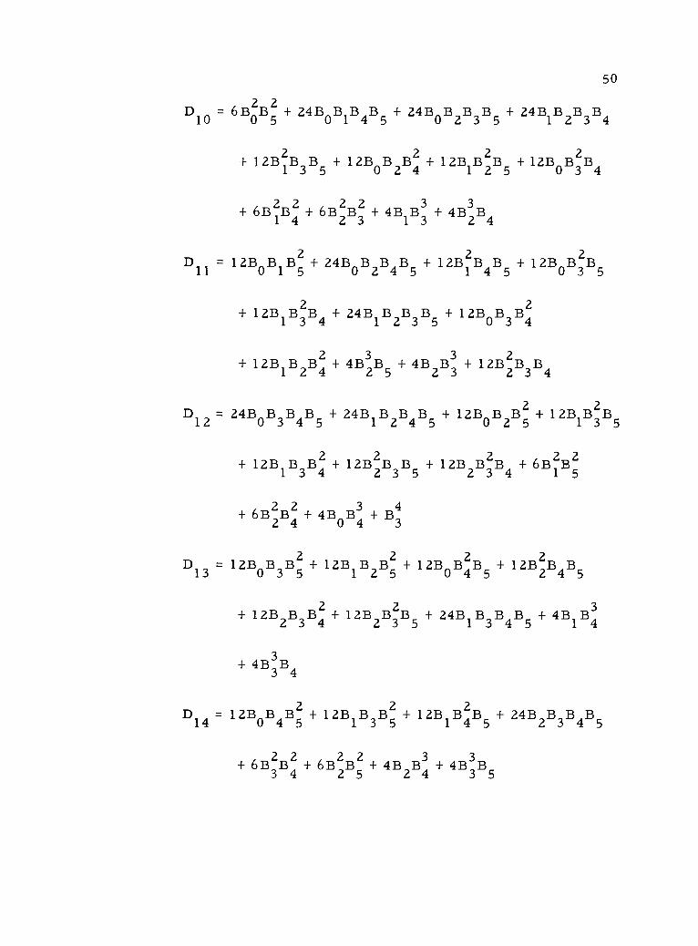
Again by use of two computer programs called "CONVO 3" and
"C ONV 0 4" the values were obtained for [ f1(t)]3 [ f2(t)]4
by knowing .A0, A1, . . . , A5 for each section. The computer
programs are in Appendix A.
So for Set B:
{GC [f1(t)] }34-2
}3 {0. 35355339 + (4. 2264026)S
(1+S)
+ (23. 557544)S2 + (80. 814188)S3
+ (190. 14209)S4 + (323. 92282)S5
+ (410. 99906)S6 + (392. 76455)57

+ (281. 55377)S8
+ (148. 03460)59
+ (54.155596)S10
+ (12.1655851)S11
+ (1. 0957813)S12
(0. 093838570)S13
+ (0. 0020079207)S14
(0. 000013517523)515}
{L [ f2(0 4-2] 1 4= { }4 {0. 25 + (5. 0079315)S + (46. 613858)S
2
(1+S)
+ (268. 82350)S3 + (1079. 0363)S 4
+ (3204. 1002)S5 + (7288. 3963)S6
+ (12953. 243)S7
+ (18154. 257)S8
+ (200800. 821)S9 + (17401. 922)S10
+ (11619. 7)S11 + (5807. 7446)S12
+ (2071. 3252)S13 + (483. 6146)S14
+ (63. 198096)S15 + (2. 3983112)S16
- (0. 20143417)S17 + (0. 0039526217)&8
- (0. 00003172817)S19
+ (0. 0000000926578205201
52
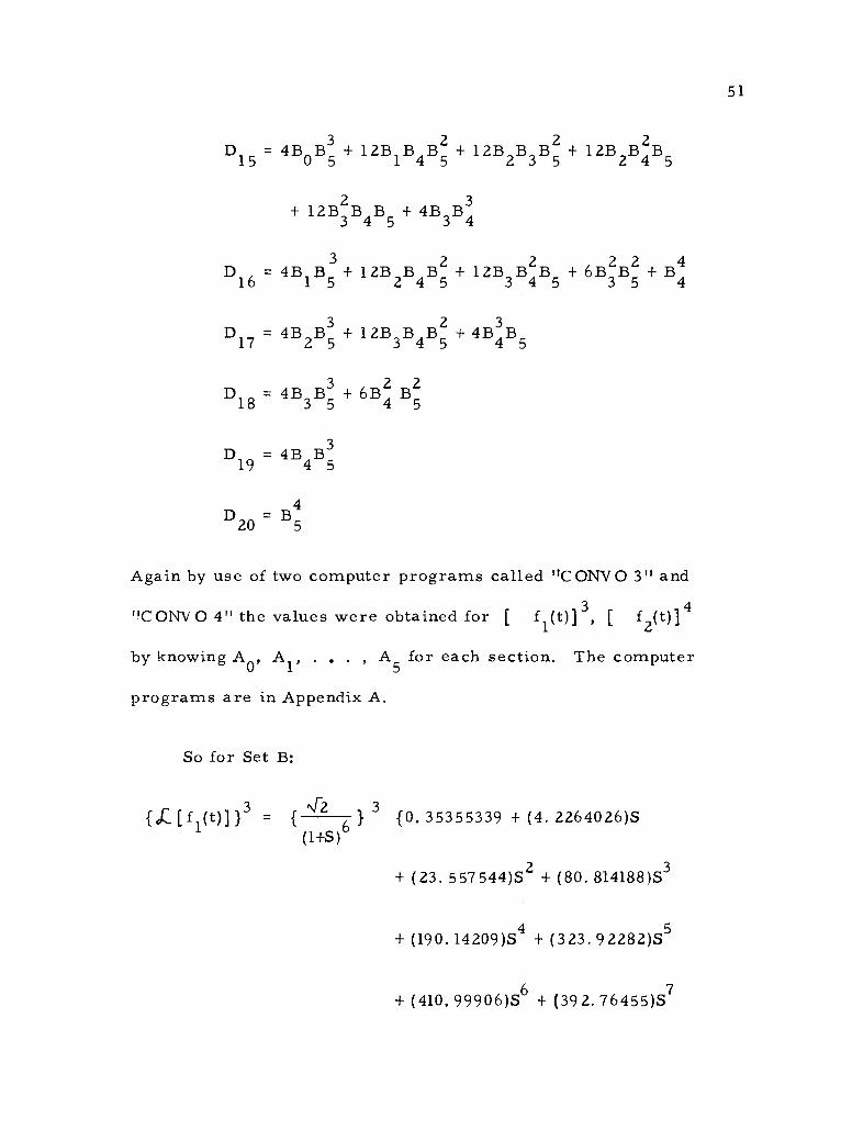
Now calculate
4-2 4
VEl2(t)114 1+S
fsk [fi (OW 2 3
(1+S)
0. 25 + (5. 0079315)S+ (46. 613858)52 + . . .
0. 35355339 + (4. 2264026)S + (23. 557544)52..
After dividing and throwing away all the terms after S5,
{4 [f2(t)] }4 ,4-2[ O. 70710678 + (5. 7117641)S
[fl (t)] }- (1+S)
Or:
+ (16. 449975S 2 + (21. 495731)S3
+ (13. 076777)S4 (5. 7708116)55]
1- [1. 0000000 + (8. 0776543)S(1+S)-
+ (23. 263778S2 + (30. 399554)S 3
+ (18. 493355)S4(8. 16116)55]
53
54
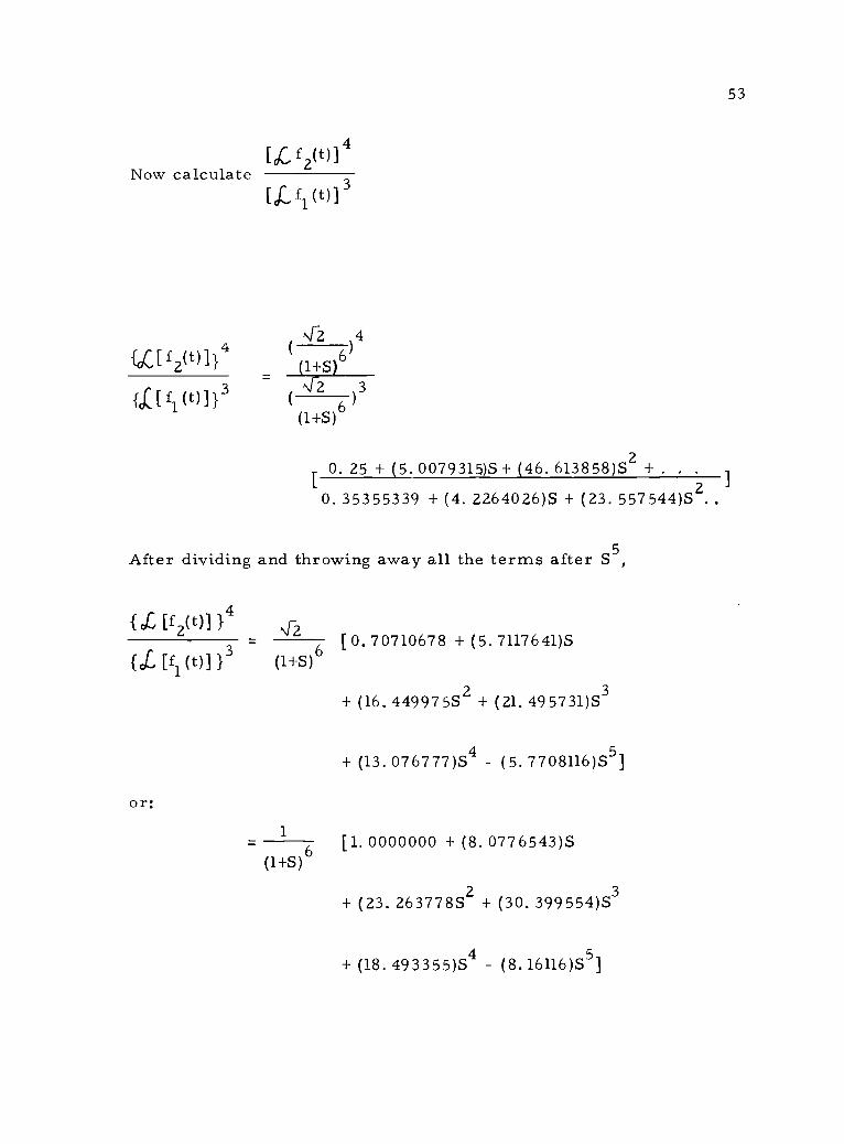
but it was earlier shown that
[ f5(0] - 1 [1. 0000000 + (5. 2225050)S(1+S)
+ (7. 9903209)S 2 + (7. 8138965)S3
+ (0. 018980490)S4
+ (0. 037952272)S51
Now invert
[aC f2(t)] 4
[oG fl (0] 3
from previous calculations, it was shown that
BO = AO + Al = A2 + A3 + A4 + A5
B1 = 5A0
+ 3A1
+ A2 A3 - 3A4
- 5A5
B2 = 10A0
+ 2A1
- 2A2
2A3
+ 2A4
+ 10A5
B3 = 10A0
- 2A1
2A2
+ 2A3
+ 2A4
-10A5
B4 = 5A - 3A1
+ A2 + A3 - 3A4
+ 5A5

55
so by some basic algebra one can get:
1AO = 32 [BO + B1 + B2 + B3 + B4 + B5]
1Al =-32 [5B0
+ 3B1
+ B2 - B3 3B4 5B 5]
1A2 = 3 [10B0
+ 2B1
- 2B2
2B3
+ 2B4
+ 10B5]
1A3 =-3 [10B0
2B1
2B 2+ 2B3
+ 2B4 10B 5]
1A4 = 32 [ 5B0 3B1 + B2 + B3 3B4 + 5B5]
1A5 =72 [BO - B1 + B2 B3 + B4 - B5]
For simplicity, program "INVERSE" was used which gave
values of A0, A1, . . . , A5 by knowing B0, B1, . . . , B5. Then
again by using program "DATAGEN 5" and "PLOTTER 5" the nor-
mal curve for section 5 and also the curve for inverting
[Jf2(t)]4
[GC, fl fit)] 3
were plotted in Figures 16 and 17.
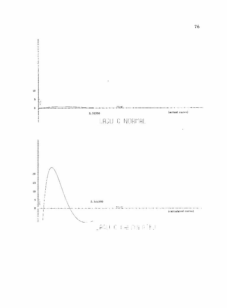
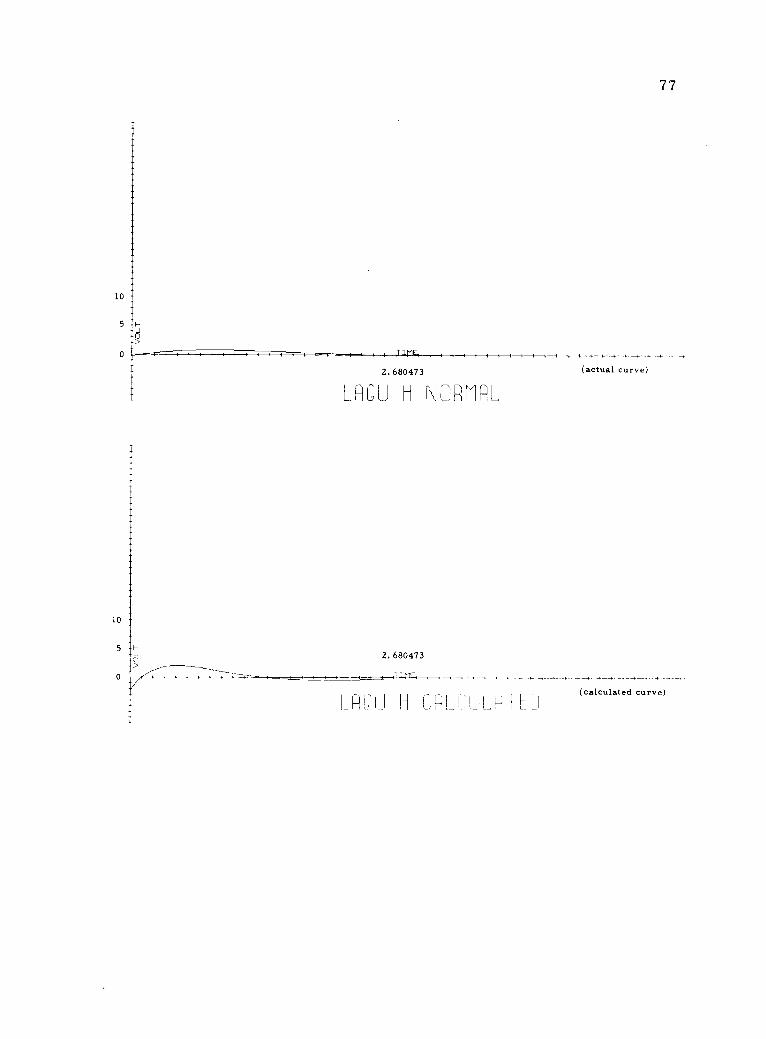
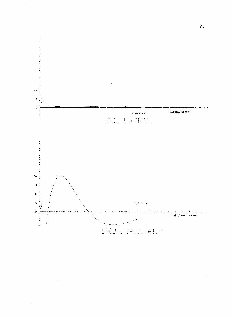
As it is seen for set B, the two curves are completely dif-
ferent so it was concluded that the residence time distribution in
one section is not independent of the RTD in the second one.

2.6584
Figure 16. LAGU B NORMAL
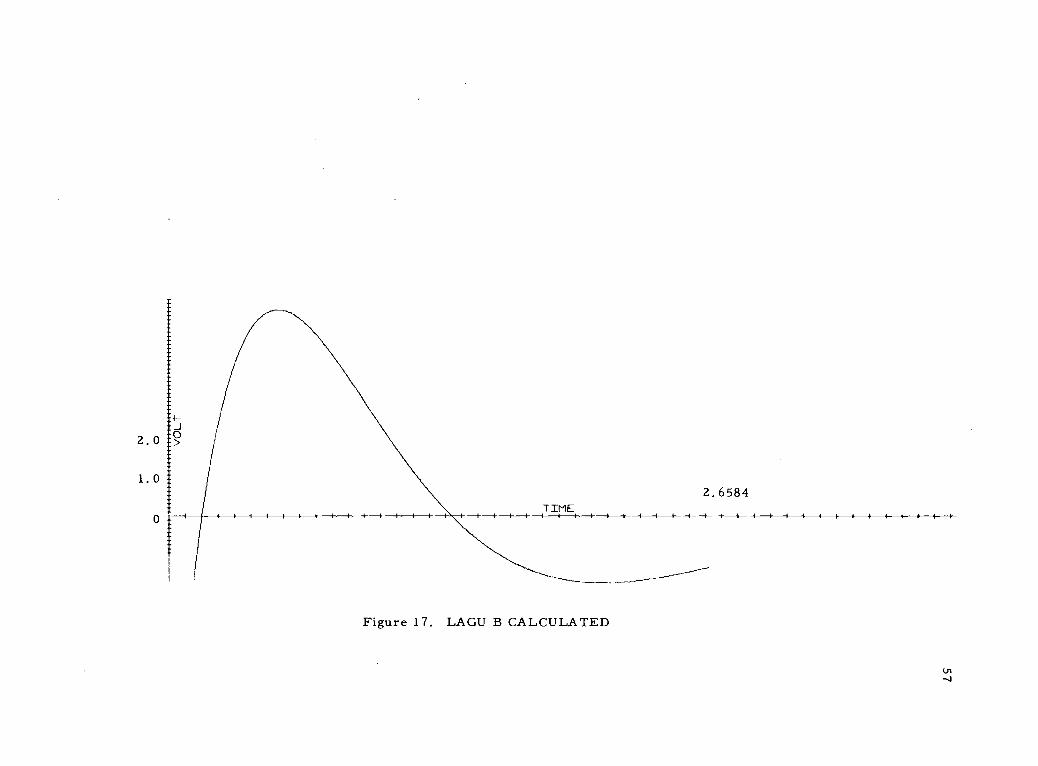
2.6584TIME1111 11111111141 1111 1111 11111111111111 1111
Figure 17. LAGU B CALCULATED
58
RESULTS
The same data analysis procedure was followed for the other
sets and the following results were determined:
Set A
Set B
Set C
Set D
Set E
Set F
Set G
Set H
Set I
Set K
Set L
Set M
do not convolute
do not convolute
do not convolute
do not convolute
do not convolute
do not convolute
do not convolute
do not convolute
do not convolute
do not convolute
do not convolute
do not convolute
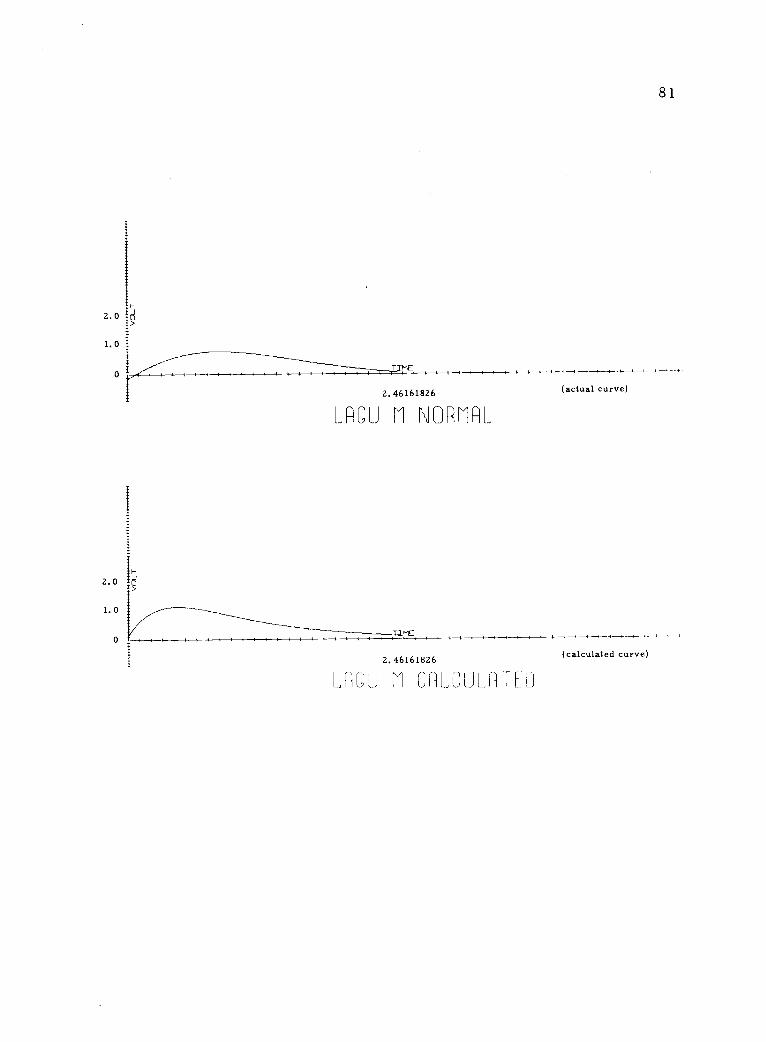
the final curves for each set of data are presented in Appendix B.
59
CONCLUSION
In all of the cases investigated the residence time distribution
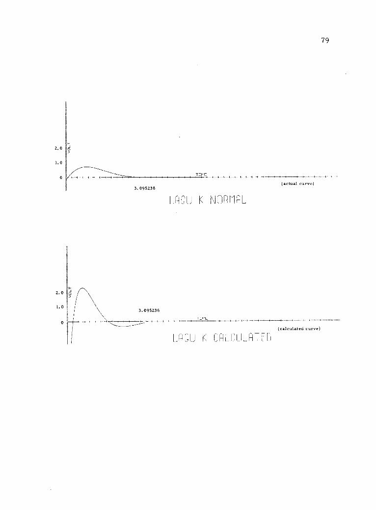
of each of the individual sections were found to be dependent upon the
preceding sections; i. e. , not independent of each other. Even though
the graphs of set L and M initially indicate independence between
the sections, evaluation of the dead time for each graph of these
two sets proved that there is dependency between the sections. In
the case of independence, (as indicated by the existence of convolu-
tion), the following relationship of dead time must be satisfied.
4 dead time for graph obtained after second section
-3 dead time for graph obtained after first section
= dead time for graph obtained after fifth section .
For set L, the dead time relationship is 4(9.6)-3(5.2)=.8
sec, while the actual dead time for 5th section, set L is 27.6 sec,
and for set M, 4(26.4)-(13.6) = 64.8 sec, while the actual dead
time for 5th section, set M is 166 sec.
Since no independence existed for all of the cases investi-
gated, the residence time distribution of each of the individualized
sections were also dependent upon each other. This interdependency
indicates that deviation from convolution always existed. Because
of this dependency there is no way to evaluate the residence time
60
distribution in a single section. A direct flow visualization will
be necessary to find the type of coupling which exists between
the flow patterns in adjacent sections.

61
BIBLIOGRAPHY
1. Geddes, L. A. , "Electrodes and the measurement ofbioelectric events,,, (1972).
2. Hellinckx, L. J., H. M. Olin and J. Rijckmans, "Residencetime distributions in compartmented reactors, " Proceedingsof the Fifth European Symposium on Chemical ReactionEngineering (1972).
3. Khang, S. J. and Fitzgerald, T. J. , HA new probe and circuitfor measuring electrolyte conductivity', Industrial andEngineering Chemistry Fundamentals May (1975).
4. Leruch, V. G., Markin, V. S. and Chirmadzhen, Yu, A.,"On hydrodynamic missing in a model of a porous mediumwith stagnant zones,H Chemical Engineering Sci., Vol 22(1967).
5. Levenspiel, 0. , "Chemical Reaction Engineering, HJohn Wiley and Sons, Inc., New York (1962).
6. Schwan, H. P., "Electrode polarization impedance andmeasurements in biological materials,,, Ann. N. Y.Acad. Science (1968).
7. Solodovnikov, V. V. , "Introduction to the statisticaldynamics of automatic control systems, I, Dover Publi-cations, New York (1960).
8. Veeraraghavan, S. and T. L. Silveston, Canadian Journalof Chemical Engineering, Vol. 49 (1971).
9. Wen, C. Y. and Cheng, S. F., "Dynamic response equa-tion for various reactor models', Canadian Journal ofChemical Engineering, Vol. 43 (1965).
10. Zwietering, T. N. , "The degree of mixing in continuousflow systems,H Chemical Engineering Science Vol. 11,(1959),

APPENDICES

62
NOMENCLATURE
A Laguerre coefficient
d baffle orifice diameter
D pipe diameter
E age distribution function
F,f Laguerre polynomial
G age spectrum generating function*
G conditional probability
h dead time
1 length of each section
L Laguerre function
M digitized points number starting after dead time
N digitized points number starting after injecting tracert time
t time of backmixing
v volumetric flow rate
volume of each section
shifting time
63
APPENDIX A
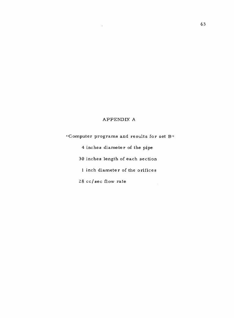
It Computer programs and results for set B"
4 inches diameter of the pipe
30 inches length of each section
1 inch diameter of the orifices
28 cc/sec flow rate

PROGRAM LISTERCC BEHROOZ SATVAT / OSU CHEMICAL ENGINEERING PROGRAM EDITORC JUNE 20, 1974 CC BEHR001 SATVAT / OSU CHEMICAL ENGINEERING.
INTEGER COUNTER, BUFF, OUTUNIT " JUNE 20. 1974DIMENSION BUFF(22) CDATA (INUNIT=1), INTEGER BEGINOXoENDIROX,POINTERO,BUFFOUTUNIT(OUTUNIT=2), DIMENSION 0UFF122)IBUFF=1, DATA (POINTER=1),(LENGTH=10001
2, WRITE (61 0000)3, NOFG=FFINI60/41 DO 70 I1 =14140FG5 OUTUNIT=I1A161; CALL EQUIP tOUTUNIT0HFILE 1
7, WRITE 1610001) Ila, NOFS=FFIN(60)9, DO 60 I2=100FS10, WRITE (6100021 1211, BEGINDX=FFIN(60)12, 10 IF (POINTERBEG/NOXI 3094092013, 20 STOP 0000114, 30 P=O
INTER=POINTER+1
16oGO
FTN1101
40 IF (I2eLTeNOFS) GO TO 4518, WRITE 12194 ENDINDX=FF Nt60)20, LENGTH=END NDX-.41EGINDX.121, 45 MAX=POINTE +LENGTH22) FLAG=0
WRITE COUTUNIT,200)BUFF 47 00 50 14=1,22COUTNER=0 IF (POINTER.LT.MAX) GO TO 49
10 00 20 1=1,22 FLAG=1BUFF(I)=FIN(INUNIT) GO TO 55IF (BUFF(DoE0o99999) GO TO 30 49 BUFF(I4)=FIN(1)
20 CONTINUE 50 POINTER=POINTER.1WRITE (OUTUNIT,100)COUNTER,BUFF 55 J=14..1COUNTER=COUNTER+22 WRITE (OUTUNIT0003)(BUFF(I),I=toJ)GO TO 10 FI 4oNOToFLAG) GO TO 47
30 J=..-1 60 CONTINUEWRITE (OUTUNIT,1001COUNTERo(BUFF(I),I=1,J) ENOFILE OUTUNITSTOP WRITE (610005)11OUTUNIT
100 FORMAT (* $15*/*2215) 70 LENGTH=1000 ,
200 FORMAT (*1*6X,110(**//* *6)(022151$ $6X,110(**)/1 STOPENO 9000 FORMAT l* NUMBER OF GRAPHS A*1
9001 FORMAT (* NUMBER OF SETS IN GRAPHII2* A*)9002 FORMAT 1* INDEX c THE 1ST ELEMENT OF SET*I2* A*19003 FORMAT (2215)9004 FORMAT I* INDEX OF THE LAST ELEMENT OF SET*I2
* (LAST SET) AA9005 FORMAT (*-11DITTED FILE OF GRAPH*I2* IS WRITTEN*
* ONTO LUN*I2)END

PROGRAM SATVATIO PROGRAM SATVAT2BDIMENSION P(2500) DIMENSION P(2500)READ(2.10) (P(N),N=1.2500) READ(2.10) (P(N)04=1.2500)
10 FORMAT(22F5.0) 10 FORMAT(22F5.0)WRITE(3.100) (P(NI.N=1001.100E) WRITE(3.100) (P(N).W1.20)
100 FORMAT(4X.5E10.3) 11.40 FCRMAT(4X.5E10.3)AREA0=0. AREA0=0.AREA1=0. AREA1=0.AREA2=0. AREA2=0.AREA3=0. AREA3=0.AREA4=0. AREA4=0.AREA5=0. AREA5=0.1.1=210. 12=490.00 50 N=L1.2500 00 50 N=12.2500M =(. -L1 M=N-L2XM=M XM=4THETA=XM/335. THETA=XM/605.W =EXP(- THETA) W=EXPI-THETA)V=SORT(2.0) Y=SORT(2.0)FLO=(W).(Y) FLO=01).(Y)FL1=(W).(THETWHETA-1.).(Y) FL1=01).(THETA+THETA-1.).(Y)FL2=(W).(THETA.(THETA+THETA-4.)+1.).(Y) FL2=01).(THETA.(THETA+THETA-4.)+1.).(Y)FL3=(W).(THETA.(THETA.((4./3.)+THETA-6.)+6.)-1.).(5) Fl3=(W).(THETA.(TMETA(14./3.)*THETA-6.)+6.)-1.).(Y)FL4=(W),ITHETA.(THETA.(THETA((2./3.)THETA-(16./3.)) FL4=(W).(THETA.(THETA.(THETA.((2./3.)*TMETA-(16./3.))5+12.1-8.1.1.1(V) '4.12.1 -8.1+1.1.(5)FL5=04).(THETA(THETA.(THETA*(THETA.(14./15.).THETA FL5=(W).(THETA.(THETA*(THETA.(TMETA.4(4./15.).THETA-.-(10./3.))*(40./3.))-20.)4.10.)-1.).(V) .S-(10./3.))4.(40./30)-20.1,10.)-1.).(Y)PR000=1P(N)/100.).(FLO/335.) PRODO=(PIN)/100.).(FLO/605.)PRO01=(P(N)/100.).(FL1/335.) PROD1=(P(N)/100.),IFL1/605.)PR002=(PIN)/100.)*(FL2/335.) PROD2=(P(N)/100.)*(FL2/605.)PROD3=(P(N)/100.).(FL3/335.) PROD3=(P(N)/100.)*(FL3/605.1PROC14=(P(N)/100.).(FL4/335.) PROD4=(P(N)/100.).(FL4/605.)PR005=(P(N)/100.).(FL5/335.) PROD5=(P(N)/100.)*(FL5/605.)AREAO=AREA04,PRODO AREAO=AREAO4PRODOAREA1=AREAIIPROD1 AREA1=AREA1+PROD1AREA2=AREA2+PROD2 AREA2=AREA2+PR002AREA3=AREA34FR003 AREA3=AREA3+PROD3AREA4=AREA40,0004 AREA4=AREA4+PR0D4
50 AREA5=AREA5+PR0D5 50 AREA5=AREA5+PROO5WRITE(3.201 AREAO.AREA1.AREA2.APEA3.APEA4.AREA5 WRITE(3.20) AREAO.AFEA1.AREA2.AREA3.AREA4.AREA5
20 PORMAT(3)(AREA0=t.E20.9///3X.YAREA1=*,E20.9////3X. 20 FORMATI3X.WAREAO=S.E20.9//3X.*AREA1=i.E20.9///3X..1*AREA2=*.E20.9///3XSAREA3=t.020.5/1/3X. 5tAREA2=XtE20.9///3X.tAREA3=$.E20.9///3X.5XAREA4=$.020.9///3X.*AREA5=0.020.9) SWAREA4=$.E20.9///3X.WAREA5=$.020.91ENC ENO
PROGRAM SATVAT5BDIMENSION P(4890)READ(2.10) (PIN).N=1.4090)
10 FORMATI22F5.0)WRITE(3.100) (P(N).W2150.2160)
IGO FORMAT(4X.5E10.314REA0=0.4REA1=0.AREA2=0.4REA3=0.AREA4=0.AREA5=0.L5=1520.DO 50 N=15.4090M=N-15XM=MTHETA=XM/1250.W=EXP(-THETA)Y=SQRT(2.0)FLO=(W)*(Y)F11=(W)(THETWHETA-1.).(Y)FL2=($4) (THETA.(THETA+THETA-4.)+1.)(5)FL3=(W).(THETA.(THETA.1(4./3.)THET4-6.14.6.)-1.).(5)FL4=(W).(TMETA.(THETA.(THETA((2./3.)*THETA-(16./3.))s+12.)-8.)+1-1.(5)Fl5=(W1.(THETA.(THETA(THETA.(THETA.114./15.)*THETA(10./3.))4.(40./3.))-20.)+10.)-1.).(5)
PR0D0=(P(N)/100.)(FLO/1250.)PROD1=(P(N)/100.).(FL1/1250.)PR002=(P(N)/100.)*(FL2/1250.)PR003=(P(N)/100.)*(FL3/1250.)PR004=(P(N)/100.).(FL4/1255.)PROD5=(P(N)/100.).(FL5/1250.)APEAO=APEA04-00000AREA1=AREA14.PR001AREA2=AREA2+PROO2AREA3=AREA3+PR0D3AREA4=AREA44.RR004
50 AREA5=AREA5.PR0D5WRITE(3.20) AREAO.APEA1,AREA2,APEA3,AgEA4,APEA5
20 FORMAT(3X.tAREA0=f,E2C.9///3X.FAREA1=t.E2C.9///3X.StAREA2=2.E23..///30./AREA3=1.122.9///3X.I(AREA4=*.E20.9///3X.200E05=0.020.9) a"ENO LIT
PROGRAM DATAGEN1B PROGRAM DATAGEN2BDIMENSION BUFFER (101 DIMENSION BUFFER (10)F03=4./3. F03=4./3.103=2.13. 103=2.13.SIXT03=16./3. SIXTD3=16./3.F015=4.115. F015=4./15.TEN03=10./3. TEND3=10./3.FORTY03=40./3. FORTYD3=40./3.AO=FFIN(48) AO=FFIN(481A1=FFIN(481 A1=FFIN(48)A2=FFIN(481 A2=FFIN(48)A3=FFIN(48) A3=FFIN(48)A4=FFIN1481 A4=FFIN(481A5=FFIN148) A5=FFIN(48)SORT2=SORT(2.01 SORT2=SORT(2.0)T=0.0 T=0.0
1000 0 1=1.10 10 00 20 1=1.10T2=T2T T2=T.TT3=T2.1. T3=T2.1T4=73.1 T4=131.15=147 15=74.1Y=SORT2EXP1-TI Y=SORT2EXP(-71
(A0+111.1T+T-1.0).A2.(1"212-4.0.11.01 (A0011.(T.T-1.01+A2.(T2442-4.0T+1.0)r63(F03'13-6.012+6.01-1.01 +113(F0313-6.0.124.6.07-1.0)4(4(10314-SIXTD31312.012-8.0.1 rA4 (103+14-SIO(10313+12.0.12-15.01+1.0) +1.01.(15(F015T5-TEND3T4FORTY03,(3 A5.(F015T5-TEND3T4FORTYD3T3-20.01*T+10.0.1-1.01) -20.0*T.T.10.0.T-1.0)1
BUFFER(I)= 5.100.0 BUFFER(I)=Y.100.01=7+0.002985 1=1+0.0016529IF(T.GE.6.7013251 ;0 TO 30 IFIT.GE.3.07935) GO TO 30
20 CONTINUE 20 CONTINUEWRITE (2.100) BUFFER WRITE (2.100) BUFFERGO TO 10 GO TO 10
30 J=I-1 30 J=I-1WRITE (2.100)(BUFFER(I),I=1.J) WRITE (2.100)(BUFFER(I),I=11)STOP STOP
100 FORMAT (5E14.61 100 FORMAT (5E14.61ENO END
PROGRAM DATAGEN5BDIMENSION BUFFER (101FD3=4./3.103=2./3.SIXTD3=16./3.F015=4./15.TEND3=10./3.FORTY03=40./3.AO=FFIN(48)AI=FFIN(48)A2=FFIN(481A3=FFIN(48)A4=FFIN(481A5=FFIN(48)SORT2=SORT(2.0)1=0.0
10 DO 20 1=1.1012=TTT3=T2TT4=1"3T15=T4.1"Y=SORT2EXP1-T1
(A0+1111144-1.0A2(T24J2-4.0.7+1.01+03(F03.13-6.0.12+6.0.1-1.01114.(103.T4-SIXT93T3.12.012-8.0T
+1.0).115.(F015.15-TE403.14+FORTY0313-20.0.1.1+10.0.T-1.011
OUFFER(I1=Y100.0T=T+0.0008IF(T.GE.2.6584) GO TO 30
20 CONTIN UE2WRITE 1.100 SUFFER
GO TO IU30 J=I-1
WRITE 12.100118UFFER(I1.1=1,11STOP
100 Fry?mAT (5E14.61END
CN

PROGRAM PLOT19 PROGRAM PLCT2BINTEGER TEMP1.YESNO INTEGER TEMP1.YESNOWRITE (61.100) WRITE (61,1001
10 READ (60. 200) YESNO 10 READ I60,2001YESNOIF (YESNO.EQ.ANO A) STOP 1 IF (YESNO.EQ.ANO A) STOP 1IF (YESNO.EQ.AYES A) GO TO 15 IF (YESNO.EQ.AYES *1 GO TO 15GO TO 10 GO TO 10
15 CALL PLOTLUN (3) 15 CALL PLOTLUN (3)CALL ERASE CALL ERASECALL FSCALE (.4.2..5..00.1 CALL FSCALE (.4.2.5..80.1CALL AXIS (-10..2471..-40.310..100..10.) CALL AXIS (-10..2371..-40.,310..100.,10.)REWIND 1 REWIND 1
XX=0.0 =0.020 Y =FIN(1)FI=20 Y
CALL PLOT (X.Y,1.0) CALL PLOT (X.Y.101X=X+1.0 X=X+1.0IF (X.LE.2460.1 GO TO 20 IF (X.LE.2360.) GO TO 20CALL PLOT (1200.,10..0.0) CALL PLOT (1200.,10.,0 0)CALL WRITEY (1..0..0HTIMEX=100.
1 C(.1.11ilo0NRITEY (1.0..8HTIME )
30 CALL PLOT (X.-10.0,0.01 30 CALL PLOT (X.-10.0.0.0)TEMP1=X0.4 TEMP1=X+0.4CALL XLATE (TEMPI TEMP) CALL XLATE ITEMPI,TEMP)CALL WRITEY (1..-90..TEMP) CALL WRITEY (1.,- 90.,TEMP)
XX=X+100.0 =X+100.0IF (X.LE.2500.01 GO TO 30 IF (X.LE.2500.01 GO TO 30CALL PLOT (70.130.,0,01 CALL PLOT 170..130..0.0)CALL WRITEY (1..90..8HVOLT 1 CALL WRITEY (1..90.05HVOLT 1
CALL PAGE CALL PAGECALL BYENOW CALL BYENOW
100 FORMAT (A WARNING A/ 100 FORMAT (A WARNING */A BEFCRE THE RUN ALL CF THE FOLLOWING FILES,/ A BEFORE THE RUN ALL OF THE FOLLOWING FILES*/* MUST BE DEFINED AS SHC1041*/ A MUST BE DEFINED AS sHowts,i l'EOUIP.1=FIRST PLOT DATAm*/ A i!EQUIP,1=.(FIRST PLOT DATA'$/A ?!EQUIP,3=PLOTf/ *
A ?LABEL,3/cYOLR NAME)*// AtEQUIP.3=PLOTA/?LABEL.3/4YOUR NAMEm*//
AREADY+A) AREADYmA1200 FORMAT (Al.) 200 FORMAT (A4)
END ENDPROGRAM PLOT58INTEGER TEMP1,YESNDWRITE (61,1001
10 READ (60.200)YESNOIF (YESNO.ECI.ANO *1 STOP 1IF (YESNO.ED.AYES A) GO TO 15GO TO 10
15 CALL PLOTLUN (3)CALL ERASECALL FSCALE (.2.2..5.00.1CALL AXIS (-10.4041..-40..310..100..10.)REWIND i
20 Y=FIN(1)CALL PLOT (X0.1.0)X=X+1.0IF (X.LE.4030.1 GO TO 20CALL PLOT 12300..10.90,01CALL WRITEY (1..0.HTIME )
X=100.30 CALL PLOT (X.-10.0,0,0)
TEMP1=X*0.4CALL XLATE (TEMP1,TEMP1CALL WRITEY (1..-90..TEMP1X=X+100.0IF (X.LE.5000.0) GO TO 30CALL PLOT (70.,130..0.0)CALL WRITEY (1..90.0HVOLT )
CALL PAGECALL BYENCM
100 FORMAT (A WARNING */A BEFORE THE RUN ALL CF THE FCLLCWIMG FILES,/A MUST BE DEFINEC AS SHCWNI$/A ?EOUIP.1.<F/PST PLOT DATAm*/A .EOUIP.3=PLOTA/A 2LAREL.3/<YOUP NAMEm*//AREADY.A)
200 FORMAT (A4)ENO

PROGRAM PLOTTERIB PROGRAM PLOTTER2BINTEGER YESNO INTEGER YESNOWRITE (61,100) WRITE (61,100)
10 READ (60.200)YESNO 10 READ (60.200)YESNOIF (YESNO.EQ.*NO *) STOP 1 IF (YESNO.EQ.tNO I) STOP 1IF (YESNO.EQ.*YES *) GO TO 15 IF (YESNO.E0.*YES *) GO TO 15GO TO 10 GO TO 10
15 CALL PLOTLUN (3) 15 CALL PLOTLUN (3)CALL ERASE CALL ERASECALL FSCALE (.4.2..5..00.) CALL FSCALE (.4.2..5..80.)CALL AXIS (-10..2471..-40.,310.,100.,10.) CALL AXIS (-10..2371..-40..310.,100..10.)REWIND 1 REWIND 1X=0.0 X=0.0
20 Y.-FIN(1) 20 Y=FIN(1)CALL PLOT (X.Y.1.0) CALL PLOT (X,Y.1.0)X=X+1.0 X=X+1.0IF (X.LE.2244.) GO TO 20 IF (X.LE.1062.) GO TO 20CALL PLOT (1200..10..0,0) CALL PLOT (1200..10..0.0)CALL WRITEY (1..0..SHTIME ) CALL WRITEY (1..0..8HTIME )
X=100. X=100.CALL PLOT (X.-10.0.0.0) CALL PLOT (X,-10.0.0,0)CALL PLOT (70..170..0.0) CALL PLOT (70..170.,0,0)CALL WRITEY (1.00..0HVOLT I CALL WRITEY (1..90..8HVOLT )
CALL PAGE CALL PAGECALL BYENOW CALL BYENOW
100 FORMAT (* WARNING .*/ 100 FORMAT (f WARNING v*/t BEFORE THE RUN ALL OF THE FOLLCWING FILES*/ $ BEFORE THE RUN ALL OF THE FOLLOWING FILES*/t MUST BE DEFINEC AS SHCWN(t/ $ MUST BE DEFINEC AS SHOWNWf ?!EOUIP.1=<PLCT DATA*/ t EQUIP.1=<PLOT DATA>*/t ?EOUIPO=PLOT$/ $ ?EQUIP.3=PLO1*/$ 2LABEL.3/(YOUR NAME)*// f I'LAREL.3/(YOUR NAMEs4//* READYN*) *READYN*)
200 FORMAT (A4) 200 FORMAT (A4)END END
PROGRAM PLOTTER5BINTEGER YESNOWRITE (61,100)
10 READ (60.20J)YESNOIF (YESNO.EQ.*NO *) STOP 1IF (YESNO.EQ.*YES El GO TO 15GO TO 1J
15 CALL PLOTLUN (3)CALL ERASECALL FSCALECALL AXIS (-10.,4870.,-40..310..100..10.)REWIND 1X=0.0
20 Y=FIN(1)CALL PLOT (X.Y.1.01X=X+1.0IF (X.LE.3322.) GO TO 2JCALL PLOT (2300..1)..00)CALL WRITEY t1..0..8HTIMEX=13J.CALL PLOT (X,-10.0.0.0)CALL PLOT (74.'170..0.0)CALL WRITEY 11..90..8HVOLTCALL PAGECALL BYENOW
130 FORMAT lt WARNING .E/$ BEFORE THE RUN ALL OF THE FCLLCWING FILES*/$ MUST BE DEFINED AS SHOWN((/
?EQUI'.1=sFIRST PLOT DATA>*/t l'EQUIP.3=PLOT*/t I'LABEL,3/(YOUR NAME>f//IREADY.$)
200 FORMAT (A4)EN(
50
PROGRAM CONVO1A 0=TTYIN (1.5HAO=A 1.=TT YINC15HAl=A2=TTYIN (15HA2=
3=TTYIN(15HA3=A4=TT YINC15MA4=A5=TTYIN (1511 A5=130=A0+Al+A2+ A3+A4+ A5131=15.)*(A0) 4(3. )*(A1)+A 2-A3- ( 3. )*(A4) (5. )* (A5)82=(10. )A( AO )+ )*(A/) (20* ( A2)-12.)* ( A3 )+ (2 )*( A4)
5+ (10. )* (A5)133=( 10. )*(A0 )-(2. /*IAD.- (2. )' A2)+ (20* (A3)+ (2V't A4)5.-(10.)*(A5)
B4= (5.)*(A0)-.. (3. )* ( AD+ A2+A3 13. /*OM+ (5. )* (A5)85=A0A1 +A2-...A3+A445WRITE (61. 50) 80,81,82,83,84,85FORMAT(//1)(14130=tvE14.7//1X,*81=$,E14.7//1X1482=*,
5E14.7 // /X 9*83=*, E14.7// /X, *84, E1.4. 7//1X, SB5=t95ENDE/ 4.7//)
50
PROGRAM CONVO3A 0=TTYIN(15HAO=A1=TTYIN(15MA1=A2=TTYIN(15MA2= 1
A 3=TT YIN (15MA3=A4=TraN115MA4=A5=TTYIN(15HA5=80=A0+A1 +A2+A3+A4+A581=15.1* (AO) +13. )*(A1.1+A2113-.. (3 .) 1A41 (5A* (AS)82=1/0. ),(A0)+12. 1,(011) - (20* (A2)*(2.)*(A3) (2.)*(A4)
54(10. /*(115)B3=( /0. )*(A0)-(2 PA(Al) -12.)* ( A21+12. )*(13)+12: )1114)5 (10.1*(115)F14=(5.)*(A01-13. /*( Al) +A2+A3- t3. )44(A4)+ (541* 145)85=A0-Al+A2-A3+116-ASWRITE (61950) 60,61,82,83,131,,B5FORMAT (//1)(9$60=*,E14.7//1X,*(11=#,E14.71/1X,1182,
5.E14.7//1X9*B3=i*E14.7//iXotB4***E14.7//1X9*115**95E14.7///)C0 =180)* (B0)'180/C17-(3.1*(130)*(80)*(01)C2=13./4'1E10 ) (BO )*(132)(3.)*(80)*(131)*(111)C3=(3.)*(60)(80)*(83)+ (6.1*(130)*(81)482)
5+ (1311*(81)*(81)C4=460*(130) 401131)*(831+ (3. )*(81)*(81)*(82)
1+ (3, )4((10)*(92)*(821+113.)*(130)*(00)*(94)C5=13.) 44130),1180 )*(85)*(6.11110)*(11)10141
5+ (6.)*(130)*(82)*(133).(3.118/)*(8111*(133154 (3.1 *(81)41(82)* (132)C6=(6.)*(60)*(B/),(95)+16.149(11)*(82)*(11315+ 16.1*(80)( 92) (841+(3.1*(30 1*(93)*(83)
( 3. ) 4(E11)( 81)* (041.(132)*(112)*(82 )C7=(6.)*(80)(B2)*(f15)+ (6.1*(B0)(93)(1341(6.1*(131)182)*(1341+(3.)1111),(01P,1851(3. ) 4481)* MI* (133).(3.)*(1121*(92)*(113)
C0 =46.) (80),(B3)*(135)+ 16. )41(1)11(B2 /*tintIs (6. )"(81)*(133)* (136).(3.)*(11.1* 118411* 184)54 (3. )*(82)*(132)* (84)4(3.)*(81)*(83)*(133 )C9=(6.)*(130)(BM)*(B15)4. (6.) *(8111113 /*(BS)
(6.)*(82)*(133)* (E14)+(3. )*(131),(1061* 18415+ ( 3. )*(82)*(132)* (135)+(83)*(83)*(133 )C10= ( 3.1*(130)(85),(85) +(6e) (B1)11134) (BS)
54 (6.)*( 92)*(133)* ( 85 )4(3. ) (82 )4' (114)* Mt).14 (3. )*(133)*( 83)* UMC11= ( 3. )(B1),(65)*(85) + 16. )41 (62)*(84)* IBS)
5. (3. ) *(133)*(133)*(85)4( 3. )*(83)*(84)* (134)C12= ( 3. )*(132 )*(135 ) *(n) +Me)* W3)*1134)4'1135)
5+ (WO 41134)*( 84)C13= 3. )*(83 )*(85 )4'185) + (3. )1' (134)*84)*I135)C14= ( 3. )184)*(85)*(135)C15=185)*(135)4(85)WRITE(61,200) CO,C1,C2,C3,C4,C5,C6,C7,C15,C9,C101,
SC1/9C/21,C13,C14,C15200 FORMAT(1X,ACO 14,E14.7//lAtiC1 =tip
5E14. 7//1X,SC3 =1,E16.7//1X9*C4 =*,E14.7//1X,* 5 =4.1E14.?//1X,n6 149E14.7//1X.*C7 =4,E14.7//1)(11 =it,5E14.7/Y1)(9/C9 =it ,E16.7//1X,*C10=*,E14.7//1X, *C11=lt,SE14.7//1)(91tC12=1,E14.7//1X,SC13=S,E14.7///X,*(14=*,5E14.7//1X9*C15=*,E14.7)
END
0N3 (2.hi35 '*=5VOXT//L'opT3'S=tWXT/W473.$=E110X1 /Wti35 .i.ZVOXI//L'AT3'$=TWXT//Lti3'$.01WXT//)11/1.1b0A OS
510"/ViV62VTV'OV (05.I9)31I(M CS8-178+£8-Z13416-081 *('2£/T)=5V (58*(s)+479(£)-f0+28+18+(£)-09+(5))+(2£/T)=4711 (SO.(0T)-#78+13)+£8:42)+20+(2)-T8*(2)-08+101))+V2i/*TI.EV (SO.(0T)0,9+12/+£8*(E)-28+(3)-78*(2)+08.(01))+1'3£/T)=ZV (59.(5)-10(£)-£8-28+TB+(£)+03+(5))+(2£/T)=TV (30048+£8+213+.18+00)+('ZSV'T)=0V
=SOHST)NIA11 =58 =II8NST)NIA11=110 .EOHST)NIA11.£0 =ZONST/NIA11=28 =TEINSI)NIA11=TE =09HST)NIA11=09
3S(3ANI 141/b90bd
0143 (L47135 'f=0200(W/L'hT3'$=6TWX7//i*,T3'$=OTWXT//V1135 ':=LI3OXT/W4I3.:=9TO0)(1//ihT3';=STOOXT//L4735 '$=4TOOXT//L'ht3'$=ETOOXT//L"13.$=2TO,'XT/W1+T35
`i=ITOt`XT//LhT3`$.0111,)(T//L'AT3Y= bOYXT,//L.7T35 '1= 900)(T//LAT3'4= LOY'XT//1+T3'1. 90*.XT/1247T35 'Y= X1 //Lor53'$= h0t.)(T//LAT31= £0/Xi//17733 '$= 20*.X7//L'AT3'$= TOPXS//1"7T3'$= 00$XTIJANNO3 onT
OZ0.6T0.9-10eLTO '9TOSTO47.10`£T05 '2[0`TTO`OLO`60`90.4.0.90.50`470£020`TO '00 (00T`T9)31INN
(5EI)..(58)158)+(5EI)=020 ISb) +11S8):(S9).(.70): (71=6T 0
IS9)*(S9)(478)(178)+1'9) +(S13)(S8)+ISO)+(£8)+1170 (S9)+ItO)+1,78)+14791+1/) (S9)+ISO)+(qN) :SW+ (SO).(ZU)+C";)=110 (48)(h8)+(+781+(+43)5
(58).(5e).(Fe)(£E1)(91+(513)(481 09).(£13)*( 2T) (S8)+158).(h9)*(2811+(ZT)(S8).(S9)+1S8)+(18)( ,;)=9TO (419)+13)+1A9)+(£0).141) + (S9 )+(4,13)+ (£13)+, (£9)+1'2T) +5
(Se) (ha )(78)*(39)+ l'ZI/+(S9)+IS8)+ (£B)+128)+131) +5 (SE)*(S9)+1,713)+113>+(2T) +(Sal +1S13)+(SO)+(081(h)=SIO
(SE1)(£8)+1£8)+(lii)+(h)(re)IAO)+(t8)(213)1147)+5 ISO)*ISEI)+(313)+(2131+( 9) +0,8)+(t81:1£13)+(£01+1 '9) 5 (SW+ 019 1(£0)+(28)(42)*(S13)+(tO)+ (h13)+1T8)+(2T) +5
(SID+ 198)+1 £13)+118).12T)+198 )+ ISB)(hEI )+(09)+ ('ZI)=+/TO
(78)+(£81+1£01+1£0)+ ( 7) +5 (t+2)*(h9)*(q8) (TO)+1'.71+ (Si3)+09)+ (Eel (TO):( "13) 5 (SO)+, (ill)+, (28)+120+1' 21)+1,70)+(tEll QED +IN) +( '2T) +5
101B)*(3131+(20)+12T)+1S9)(76)+ (+JO) +109)*I ZT) +5 (58)* (S8) 138)+ ITEI):( ZT)+ (SEi). (SE)+(98)+109)+('ZT)=FIG
1£81 +1i131+(F8)+ UN) +5 (1713)+178)+(halr(00): (7)+ (.76)+1,A1)+(29):(28)+ 19) +3
(S81+(SO)+(18)+1TE1)+(*9)+179)+1£01+ (Ea) (28)( ZI) +5 150)+(£8)+1291:128)+ ('ZT)+1+70 )+(781+ (£81+ (T9)+( 21) +5
(SED+ (£8 )+(£8 )*( TEI),( '21)+(Sa)(SEil (2B)+(08)+121) 45 (S8)*(,78) +129)+118): 0112) (S6)*(78)+1£13)+108)+( "72 1=ZT
(F6)+(r0):(£6)+(28)+ t "71 +5 (SO)+129)+(28)+12S)+( '471+ (478)+0713) +1ZO)*(Ii3)*( 21) +5
(.10)+076 )*(£0)+1081+ lZT)+ISE1)+1£13): (ZO)+ (TO)( t2) +5 MD+ (ZED+ (201+(213)+12T)+178)+1£9)+120)+(T9) r( 2T) +5
(SO)+(iA)+(£131108):(2T)+(S9)+1,7b):(T8)+(t8)+1211+5 (99): loal) +(OB) + ( 02)+ ( ',/2) + (Se). I S91:17131+ (M.( 21)=TT 0
148)*128)+128)+128)Wh)+(E8)*(00),(E81 ,(T9)*1..1)+5 128)1£81+128)+(20)+19)+11713)+Itli3)+ITO):(TO)+ ( 9) +5 148). (29):(£9)*( 08) +I 21)4199) +(ZS) + (28) +ITO) +I 2T) +5
11+8)*(1,9)+(Z81+(06)*(2114(SO)+1£13): (SBI ITO)+1'2I) +5 (110). (Eel+ (28)+( TO) +1172)4(913 ) *MD (Za) +(M.( h2) +5
( S8) (.7131+ (SO>+ (081+(47?)+ISO) +1S131*(09)+ ( 08)+19 )=OT 0 (£13)+128) +(38)+(28). (...?) +5
(£9)+(Z 0):(£8)*(001+ ( ") + (h9)+1£81+ (201+(013):147Z) +5 198)+1281:(T13):(08). ()21+ (28)+1£13)+ (2131+(18)+( '21)45
(S9)+(28 ).(281109)+1'21)+178)+128)+128)+118) +1 '2T) +5 (+19)+(h3)(TB)+108).(2T)+(79)+1£81 (18):(18)+(2T) +5
(S9)+120)(T13) (TO)+12T)+(SEI)+119)+1013)+(0131+ ("2T)=60 (213)+(29):(Z8)+ (all +5
(98).(T 8)*(18). I "1)+1.03 )*(£9)* (TE1)*(09)*( '4,21 45 (S9).(281+(T 8).+(00)+( 412)+ (0/81.(18) .(013 )*(011)*( 9) +5
(E8)+(f 8)+(T91+(Tb)+1'9)+1£13)+(28) (28)+ ITO) +( ZT) +5 (£0)+ (28)+( 20)+1013)+( 21)4 (478 )+(213): (281 +108)+12T) +5
1+19)(213)+IT13)+(T3):(2S)+(S8)(£13)+(09).(013)+1ZT)=90 121:11+128)120)+(113)+ ( "7)+5 (A8)+119)+II9):(TO)+(?)(1721+(28)(TO)+(09)+( 4721+5
(213)+(29 )+(T8)+( T9)+1 21) 4128 ).(213). eel+ (013)+121)+5 (£81+ (19 )+ (TO)+(n),121)+(S8)+(i6). (T8):(08)+( ZT) +5
(h8)+(£81+108)+(0a).(ZT)+(69)*(213)(013)(091+( 'ZI)=LO (38)+1313)*(28):(08)+ l'h)+1£13)+(T8)+(TB)+(t8). 11) +5
(£81+ (29)+1S9)1013)( AZ)+138)+(ZO) +UM+ ITO)+I'9) +5 (23)+(03)+108)(09)+(9)+(478)(T8)+ (S8)+(08)+( ZT) +5
1,191+(Z8)+108): (oa)*(2T).(sE) (16)(08):(08)+1'2T)=90 (28)+IT8)+(TE1)+(T8)+( 471+ (28).(39)+ (TO) (DO) +( "ZT) +5 (£8)+(T8)*(1e1 +(08)+1ZT)+(£13)+(20)+(03)+(08)*( 2T) +5
(h3)+(i3) +(08)+(013) :( ZT)41S9)*(081+ (08)+1001+ lh)=S0 (TO) +MI+ (T8 )*( T9) +5 (33)+(TO)+(i8)(08):( 2114 (Z13)+(ZO)+(03 )*(013 1, (9) +5
(£8) :(T8):(09)(091+13T)+(AO)+(08)+(081+ (DOI+ (17).:A0 (18)+(113)+(TEI)+(08)+( "7) +5
(28):(T8)+(09)(00)+1'2I)+(£81(013)+(08) 108)147)=£0 IT131+ (T6 )+(08).(08)+(' 9)+129) +(OA+ ( 081+ ( 08)+1*/)=20
I T9):(013).(08)*(09) + ('17)=T (09).109).(08) :(00) =00 I /// '47T35
'i=530XT//L'.773'$=119i'XT//P4T3.*=EBY'XT//1*,7135 '2=291'XI//L'4 T3'$=T80(IY/L'47T3'$=0BOXI//)11/W803 OS
58h81820'7000 (05.T9)31IdM SI/ -.710+VV -ZV+TV -09=S9
(511)+('S)+10/)(£)-£V+2V+(iV)+1£)-(011)+1S)=176 (99)+1 0T) -5
(*IV)+(21+(£V)+(2)412V1+021-111/1+( Z)-(0,1)+( '01)=28 (991..-( OT ) +5
1,7V)+1 2) +IEV) ( 2)-(29)+("2)- (TV)+(*2)+ (09)+IOT)=28 (SY)+('S)-(6711)+121-£V-211+(117)+( £110V)+1'S)=TS3 59+.79+09+29+19+09.08 =GVHST/NIA11=S11 =PsVHSTINIAll=hV
=EVHST)NIALL=E V =2VHSTINIA11=211
=TVHST/NIA11=T V =OVHST)NIAll=n11
ft° ANO3 WV 6908d
71
APPENDIX B
Final Results For All Sets
10
5
0 I I 4
,-----------,,
/
3. 9050
NuRn=1
(actual curve)
3.9050 (calculated curve)
L. C
72
2.0 o
1.0
73
TIME
L C
2.91715
C \OR'RL
2.91715
C CRLCULRTEfi
(actual curve)
(calculated curve)
5.0
4.0
3.0
2.0
1.0
0
74
TIME
4.087156 (actual curve)
LA, \OR'
LA
4.087156
TIME
L
(calculated curve)
-4-

L
2.836770
OR\IAL
75
(calculated curve)
0
2.32350
LP
2.322350
T1Mr
G NORL1HL
n
-4-
(actual curve)
(calculated curve)
76
10
5
O
0 4 4-,
10
5
2.680473
LRGLI \(actual curve)
R'AL
2.680473
(calculated curve)_H,171 H iL 11
77
10
20
15
10
5
LA:b
2.625579
2.625579
I -4
bL I bb ,2 L: LI r= T
(actual curve)
(calculated curve)
78
79
3.095238
(calculated curve)
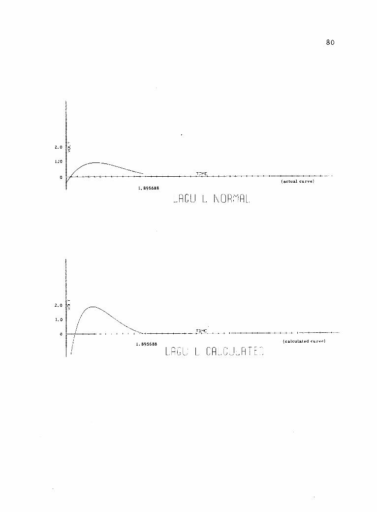
1.895688
L R- L \DR 'RL
(actual curve)
80
1.895688
LR L :Th,RL11PIT D
(calculated curve)
2.0
1.0
2.0 d
1.0
LR,_
TIME
2.46161826
\OR'AL
ME
(actual curve)
2.46161826
LAG_ CRLC_LRTE
(calculated curve)
81