Residual periodograms for regularization - NISTBRust/pubs/Unfolding/InvProbs2008.pdf · Residual periodograms for choosing regularization parameters for ill-posed problems ... Bayesian

IOP PUBLISHING INVERSE PROBLEMS

Inverse Problems 24 (2008) 034005 (30pp) doi:10.1088/0266-5611/24/3/034005

Residual periodograms for choosing regularizationparameters for ill-posed problems

Bert W Rust1 and Dianne P O’Leary1,2

1 Mathematical and Computational Sciences Division, National Institute of Standards andTechnology, Gaithersburg, MD 20899, USA2 Computer Science Department and Institute for Advanced Computer Studies,University of Maryland, College Park, MD 20742, USA

E-mail: [email protected] and [email protected]

Received 28 June 2007, in final form 6 October 2007Published 23 May 2008Online at stacks.iop.org/IP/24/034005

AbstractConsider an ill-posed problem transformed if necessary so that the errors inthe data are independent identically normally distributed with mean zero andvariance 1. We survey regularization and parameter selection from a linearalgebra and statistics viewpoint and compare the statistical distributions ofregularized estimates of the solution and the residual. We discuss methodsfor choosing a regularization parameter in order to assure that the residualfor the model is statistically plausible. Ideally, as proposed by Rust (1998Tech. Rep. NISTIR 6131, 2000 Comput. Sci. Stat. 32 333–47 ), the resultsof candidate parameter choices should be evaluated by plotting the resultingresidual along with its periodogram and its cumulative periodogram, butsometimes an automated choice is needed. We evaluate a method for choosingthe regularization parameter that makes the residuals as close as possible towhite noise, using a diagnostic test based on the periodogram. We comparethis method with standard techniques such as the discrepancy principle, theL-curve and generalized cross validation, showing that it performs better ontwo new test problems as well as a variety of standard problems.

1. Introduction

Systems of first kind integral equations,

yi ≡ y(ti) =∫ b

a

K(ti, ξ)x(ξ) dξ + εi, i = 1, 2, . . . , m, (1.1)

are routinely used to model instrument distortions in measuring an unknown function x(ξ).The Ki(ξ) ≡ K(ti, ξ) are known (previously measured or calculated) response functions of

0266-5611/08/034005+30$30.00 © 2008 IOP Publishing Ltd Printed in the UK 1

http://dx.doi.org/10.1088/0266-5611/24/3/034005

mailto:[email protected]

mailto:[email protected]

http://stacks.iop.org/ IP/24/034005

Inverse Problems 24 (2008) 034005 B W Rust and D P O’Leary

the instrument, the yi are measurements made on a discrete mesh t1, t2, . . . , tm, and the εi arerandom, zero-mean measuring errors. Discretizing gives a linear regression model

y = Kx∗ + ε, (1.2)

where y is the m-vector of measurements, K is a known m × n matrix, with m � n, andx∗ is an unknown n-vector whose components are either discrete values of x(ξ) on somemesh ξ1, ξ2, . . . , ξn, or are the unknown coefficients in a truncated expansion for x(ξ). Anexample of such a discretization is given in appendix A. The vector ε is an m-vector of randommeasuring errors satisfying

E(ε) = 0, E(εεT ) = S2, (1.3)

where E is the expectation operator, 0 is the zero vector and S2 is the positive definite variancematrix3 for ε. When the measurement errors are statistically uncorrelated, the variance matrixis diagonal:

S2 = diag(s2

1 , s22 , . . . , s2

m

), (1.4)

where s1, s2, . . . , sm are the standard deviations of the errors. When the errors are correlated,the model can be transformed to have a diagonal variance matrix by premultiplying (1.2) bythe inverse of the lower triangular Cholesky factor of S2.

Estimates of S are often readily available along with the data values y, since goodexperimenters routinely provide estimates of the error as ±1-sigma error bars on the plottedpoints. The variances can be estimated as the squares of the half-lengths of the bars}. Ananalyst who fails to use this information implicitly assumes that S2 = s2Im, where Im isthe mth-order identity matrix and s is an unknown scalar that can be, but usually is not,estimated from the sum of squared residuals for the least squares solution. Using all availableinformation on the variances can greatly improve estimates of x.

In the following it will be assumed that S is a known matrix and that the errors aresamples from a multivariate normal distribution, i.e., that ε ∼ N(0, S2). In section 2, theseassumptions will be used to rescale the problem so that the scaled errors η = S−1ε ∼ N(0, Im)

and to derive a statistical diagnostic for estimates of the solution vector. In section 3 weuse this scaling on a variant of the well-known Phillips problem [23]; the ordinary leastsquares estimate is calculated and found to be unsatisfactory. In section 4 we discussthe families of solutions formed from Tikhonov estimation and from the truncated singularvalue decomposition (TSVD), among which an acceptable estimate of the solution can often befound, and derive their statistical properties. Section 5 discusses rules for choosing among theestimates. In section 6 we illustrate these ideas on a test problem. The new diagnostics can beused to specify high-quality Tikhonov and TSVD estimates, but in both cases, the L-curve andminimum generalized cross validation (GCV) criteria give unacceptable results. In section 7we discuss how the parameter choice method can be automated, and we present results ona variety of standard test problems in section 8. In section 9 the methods are successfullyapplied to real-world measurements of the energy spectrum of neutrons produced by a certainnuclear reaction. Finally, section 10 gives a brief discussion of algorithmic considerations andof how the new method can be extended when the knowledge of the measurement errors is notas complete as might be desired.

In some important ill-posed problems, extra information is available about the solution; forexample, we might know that x(ξ) is non-negative or monotonic. Including such constraintscan be important in achieving a good solution using techniques such as penalized maximumlikelihood, Bayesian methods, maximum entropy, etc (see for example [2, 4, 19, 24, 29]), but

3 This matrix is often called the covariance matrix.

2


we do not consider such constraints here. Neither do we consider the important question ofrobustness of our methods when our assumptions on the distribution of the error are violated.

This paper is meant to be expository, providing an overview of methods for choosingregularization parameters. At the same time, it contains some original contributions. Wecompare the statistical distributions of regularized estimates of the solution and the residualfor discretized ill-posed problems; we highlight a particularly promising and underutilizedset of statistical techniques that we have found useful in judging the quality of a solution;we propose a way to automate the evaluation when necessary, and we present two new testproblems4 useful for evaluating numerical methods. Some of this material is taken from [26].

2. Properties of the model’s residual

Our linear regression model can be written as

y = Kx∗ + ε, ε ∼ N(0, S2), (2.5)

as stated in (1.2), but it is advantageous to scale it with the matrix S−1. Let

b ≡ S−1y, A ≡ S−1K, η ≡ S−1ε. (2.6)

Note that by a standard theorem of multivariate statistics [1, theorem 2.4.4], η ∼N(S−10, S−1S2[S−1]T ), so the scaled model can be written as

b = Ax∗ + η, η ∼ N(0, Im). (2.7)

As a consequence, another standard theorem [17, p 140] gives ‖η‖2 ∼ χ2(m), where χ2(m) isthe Chi-squared distribution with m degrees of freedom. The advantage of our scaling is thatwe now can see how a reasonable residual to the model should behave. Let x̃ be an estimateof x∗ and let

r̃ = b − Ax̃ (2.8)

be the corresponding residual vector. Since the regression model can also be written as

η = b − Ax∗, (2.9)

it is clear that x̃ is acceptable only if r̃ is a plausible sample from the distribution from whichη is drawn. Since

E{‖η‖2} = m, Var{‖η‖2} = 2m, (2.10)

these two quantities provide rough bounds for the ‖r̃‖2 that might be expected from a reasonableestimate of x∗: an estimate that gives

m −√

2m � ‖b − Ax̃‖2 � m +√

2m (2.11)

would be reasonable, but any x̃ with ‖r̃‖2 outside the interval [m − 2√

2m,m + 2√

2m] wouldbe suspect. These indicators can be sharpened and quantified by using percentiles of thecumulative distribution function for χ2(m).

We will see in section 5 how to use this information in choosing among a family ofpossible regularized estimates for x∗.

4 The data for the Burrus problem in section 9 and a MATLAB program for the Phillips variant defined in the appendixare available at www.cs.umd.edu/users/oleary/bwr.

3

http://www.cs.umd.edu/users/oleary/bwr


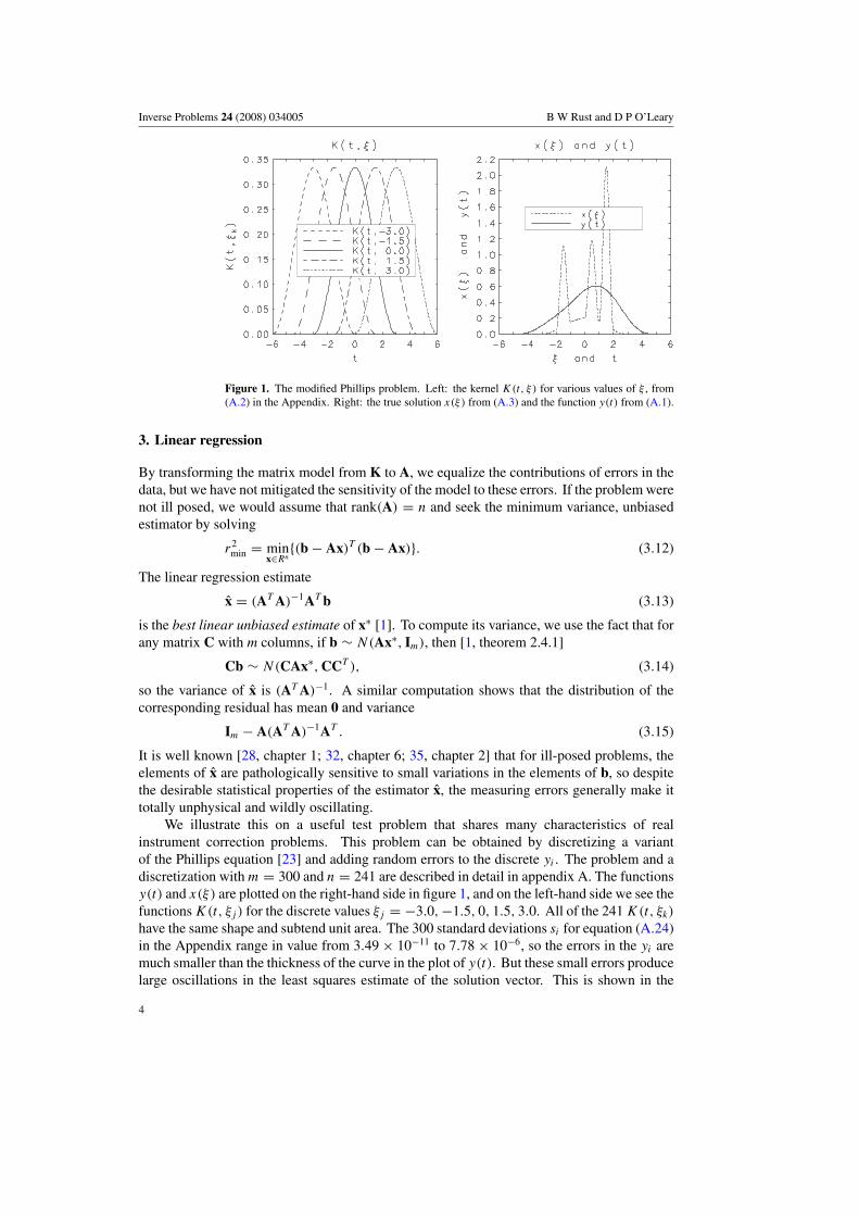
Figure 1. The modified Phillips problem. Left: the kernel K(t, ξ) for various values of ξ , from(A.2) in the Appendix. Right: the true solution x(ξ) from (A.3) and the function y(t) from (A.1).

3. Linear regression

By transforming the matrix model from K to A, we equalize the contributions of errors in thedata, but we have not mitigated the sensitivity of the model to these errors. If the problem werenot ill posed, we would assume that rank(A) = n and seek the minimum variance, unbiasedestimator by solving

r2min = min

x∈Rn{(b − Ax)T (b − Ax)}. (3.12)

The linear regression estimate

x̂ = (AT A)−1AT b (3.13)

is the best linear unbiased estimate of x∗ [1]. To compute its variance, we use the fact that forany matrix C with m columns, if b ∼ N(Ax∗, Im), then [1, theorem 2.4.1]

Cb ∼ N(CAx∗, CCT ), (3.14)

so the variance of x̂ is (AT A)−1. A similar computation shows that the distribution of thecorresponding residual has mean 0 and variance

Im − A(AT A)−1AT . (3.15)

It is well known [28, chapter 1; 32, chapter 6; 35, chapter 2] that for ill-posed problems, theelements of x̂ are pathologically sensitive to small variations in the elements of b, so despitethe desirable statistical properties of the estimator x̂, the measuring errors generally make ittotally unphysical and wildly oscillating.

We illustrate this on a useful test problem that shares many characteristics of realinstrument correction problems. This problem can be obtained by discretizing a variantof the Phillips equation [23] and adding random errors to the discrete yi . The problem and adiscretization with m = 300 and n = 241 are described in detail in appendix A. The functionsy(t) and x(ξ) are plotted on the right-hand side in figure 1, and on the left-hand side we see thefunctions K(t, ξj ) for the discrete values ξj = −3.0,−1.5, 0, 1.5, 3.0. All of the 241 K(t, ξk)

have the same shape and subtend unit area. The 300 standard deviations si for equation (A.24)in the Appendix range in value from 3.49 × 10−11 to 7.78 × 10−6, so the errors in the yi aremuch smaller than the thickness of the curve in the plot of y(t). But these small errors producelarge oscillations in the least squares estimate of the solution vector. This is shown in the

4


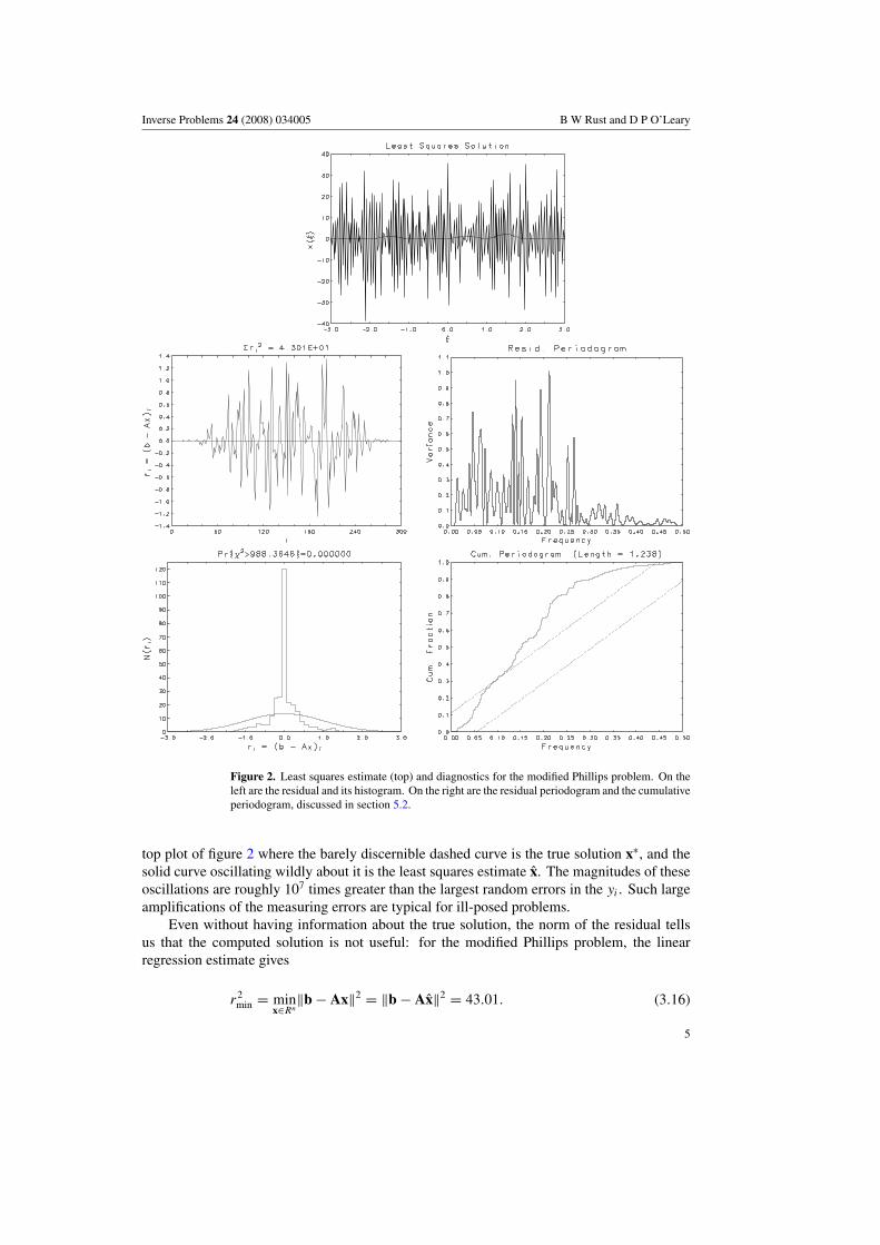
Figure 2. Least squares estimate (top) and diagnostics for the modified Phillips problem. On theleft are the residual and its histogram. On the right are the residual periodogram and the cumulativeperiodogram, discussed in section 5.2.

top plot of figure 2 where the barely discernible dashed curve is the true solution x∗, and thesolid curve oscillating wildly about it is the least squares estimate x̂. The magnitudes of theseoscillations are roughly 107 times greater than the largest random errors in the yi . Such largeamplifications of the measuring errors are typical for ill-posed problems.

Even without having information about the true solution, the norm of the residual tellsus that the computed solution is not useful: for the modified Phillips problem, the linearregression estimate gives

r2min = min

x∈Rn‖b − Ax‖2 = ‖b − Ax̂‖2 = 43.01. (3.16)

5


By (2.10), E{‖b−Ax∗‖2} = 300, with standard deviation√

600 = 24.49, so r2min is more than

10 standard deviations smaller than the expected value.To improve our estimate, we need a family of regularized solution estimates that are not

so sensitive to errors, and some means for choosing among those estimates.

4. Regularized solution estimates

Insight into the failure of the least squares method is obtained by use of the singular valuedecomposition (SVD) of A:

A = UΣVT =U[Σ1

O

]VT , Σ1 = diag(σ1, σ2, . . . , σn). (4.17)

Here σ1 � σ2 � · · · � σn � 0, and

UT U = Im = UUT , VT V = In = VVT . (4.18)

If the m × m matrix U is partitioned

U = [U1, U2], (4.19)

with U1 being an m × n submatrix, then it can be shown by substituting into (3.13) [8,section 5.5.3] that the least squares solution satisfies

VT x̂ = Σ−11 UT

1 b, (4.20)

and that

r2min = ‖b − Ax̂‖2 = ∥∥UT

2 b∥∥2

. (4.21)

These last two equations can also be written as

(VT x̂)i = (UT b)i

σi

, i = 1, 2, . . . , n, (4.22)

and

r2min = ‖b − Ax̂‖2 =

m∑i=n+1

(UT b)2i . (4.23)

Using the SVD of A, we can compute A = U1Σ1VT and

A(AT A)−1AT = U1UT1 . (4.24)

This analysis leads to two families of regularized solutions: truncated SVD (TSVD) andTikhonov regularization.

4.1. The truncated SVD family of regularized solutions

For the modified Phillips problem, the value of r2min defined by (3.16) is too small by ten

standard deviations, which suggest that some of the (UT b)i values in the sequence (4.22)more properly belong to the sum in (4.23). This reasoning leads to the idea of truncatingthe decomposition. This is accomplished by choosing a value p < n and replacing Σ1 by atruncated matrix

Σtr = diag(σ1, . . . , σp, 0, . . . , 0) (4.25)

whose pseudo-inverse is

Σ†tr = diag

(1

σ1, . . . ,

1

σp

, 0, . . . , 0

). (4.26)

6


Figure 3. Singular values (squares) and first n elements of |UT b| (circles) for the modified Phillipsproblem.

Then (4.22) and (4.23) are replaced by

(VT x̃

)i=⎧⎨⎩

1

σi

(UT b)i, i = 1, 2, . . . , p,

0, i = p + 1, . . . , n.

(4.27)

From this, we can compute

‖b − Ax̃‖2 =m∑

i=p+1

(UT b)2i . (4.28)

The above approach was first suggested by Golub and Kahan [6] who noted its similarity to thetheoretical treatment given by Smithies [27, chapter 8] for the singular functions and singularvalues of first kind integral equations. One of the first to use it was Richard Hanson [14] whosuggested that the threshold should be the smallest integer p such that

m∑i=p+1

(UT b)2i < m. (4.29)

In view of (2.10), this seems a very sensible choice. Another choice [7] is to seek a clear gapin the distribution of the σi and to zero all those on the low side. Unfortunately, most ill-posedproblems have no gap.

As an example, we see no gap in the plot of the singular values for the modified Phillipsproblem, marked with squares in figure 3, which also shows the elements of |UT b| plotted asconnected circles. The largest and smallest singular values are

σ1(A) = 2.882 × 105, σ241(A) = 2.622 × 10−2. (4.30)

with ratio (condition number) cond(A) = 1.099 × 107. The relative accuracy is εmach =2.22 × 10−16, so there is no reason to assume that the numerical rank of A is less than n. Yetthe problem obviously needs some truncation to prevent the estimate from capturing variancethat properly belongs to the residuals.

We note that the TSVD solution estimate (4.27) can also be obtained by zeroingcomponents of UT b corresponding to small singular values rather than zeroing the singularvalues of A, as noted by Golub and Kahan [6].

7


4.2. The Tikhonov family of regularized solutions

An alternative to setting small singular values to zero is to instead increase them so that theylead to a smaller contribution to the solution estimate; see (4.22). Although this strategy isgenerally attributed to Tikhonov [30], it was also pioneered by Phillips [23] and Twomey [31].A statistical variant, called ridge regression, was also independently developed by Hoerl andKennard [15, 16]. In the Tikhonov method, we add a small increment to each singular value.For the large singular values this has little effect, but for the small ones it can greatly diminishthe noise contributed by the components of U1

T b corresponding to those values.The Tikhonov regularization estimate is given by

x̃λ = (AT A + λ2In)−1AT b, (4.31)

where λ is a parameter chosen to balance the competing demands of fidelity to themeasurements and insensitivity to measurement errors. This interpretation of λ comes fromthe fact that the vector x̃λ is the solution to the minimization problem

minx

‖b − Ax‖2 + λ2‖x‖2. (4.32)

Using the SVD, it can be computed as

(VT x̃)i = σi

σ 2i + λ2

(UT b)i, i = 1, 2, . . . , n, (4.33)

which can be compared to the TSVD value (4.27). The corresponding residual norm-squaredis

r̃2min = ‖b − Ax̃‖2 =

n∑i=1

(λ2

σ 2i + λ2

)2

(UT b)2i +

m∑i=n+1

(UT b)2i , (4.34)

which compares to the TSVD value (4.28).

4.3. The statistical distributions of our estimators

In this section we use the SVD of the matrix A to derive formulas for the means and variancesof the estimators obtained from least squares and from our regularized algorithms. We willrepeatedly make use of several useful properties of the SVD. First, since the columns of U andV form orthonormal bases, we have the properties UT U = Im and VT V = In. Second, sinceΣ is an m × n matrix that is nonzero only on the main diagonal, we will call its top n × n

block Σ1 and denote the n × m pseudo-inverse of Σ by

Σ† = [Σ†1 0

], (4.35)

where the pseudo-inverse of a square diagonal matrix is formed by replacing the nonzerodiagonal entries by their inverses. To make expressions simpler we will assume that A andtherefore Σ1 are full rank so that Σ†

1 = Σ−11 and Σ†Σ = In. We will also make use of the

partitioning of U in equation (4.19), and the fact that diagonal matrices commute. We havethree kinds of solution estimates for problem (1.2): the least squares estimate, the TSVDestimate and the Tikhonov estimate. Referring to equations (4.22), (4.27) and (4.33), we seethat all of these estimates have a similar form. In fact, for all of them,

VT x = FΣ†UT b, (4.36)

8


where F is an n × n diagonal matrix specific to each method. The entries of F are called filterfactors [11]. For the ordinary least squares estimate, F is the identity matrix. For Tikhonovregularization, the j th diagonal element of F is

fj = σ 2j

σ 2j + λ2

. (4.37)

For TSVD, the first p diagonal entries of F are 1 and the others are zero.So in each case we can write the solution estimate as

x = VFΣ†UT b≡ Cb. (4.38)

From this we see that under the assumption that b ∼ N(Ax∗, Im), x has a normal distribution.We can compute the mean and variance of the distribution by using (3.14). We see, by settingC = VFΣ†UT and b∗ = Ax∗, that the mean of x is

Cb∗ = VFΣ†UT Ax∗ (4.39)

= VFΣ†UT UΣVT x∗ (4.40)

= VFVT x∗ (4.41)

= x∗ − V(In − F)VT x∗, (4.42)

and the variance of x is

CCT = VFΣ†UT U(Σ†)T FVT (4.43)

= VF2(Σ2

1

)−1VT . (4.44)

We see from these expressions that x is a biased estimator if F �= In, i.e., if we use a Tikhonovestimate with λ �= 0 or a TSVD estimate with p < n. We also see that the variance of theestimator decreases as the filter factors decrease. Therefore the variance decreases as theTikhonov parameter λ increases and as the TSVD parameter p decreases.

We can make a similar computation for the residual. Let F̆ denote the m × m matrix thatis zero except for the matrix F in its upper left block. In terms of F and the SVD of A, theresidual can be expressed as

r = b − Ax (4.45)

= b − (UΣVT )VFΣ†UT b (4.46)

= U(Im − F̆)UT b (4.47)

= U2UT2 b + U1(In − F)UT

1 b. (4.48)

Note that U2UT2 b is the residual for least squares. Since r = Cb, where we redefine

C = U(Im − F̆)UT , we see that r is normally distributed with mean

CAx∗ = U(Im − F̆)UT UΣVT x∗ (4.49)

= U(Im − F̆)ΣVT x∗ (4.50)

= Ax∗ − U1FΣ1VT x∗ (4.51)

= U1Σ1VT x∗ − U1FΣ1VT x∗ (4.52)

= U1(In − F)Σ1VT x∗. (4.53)

9


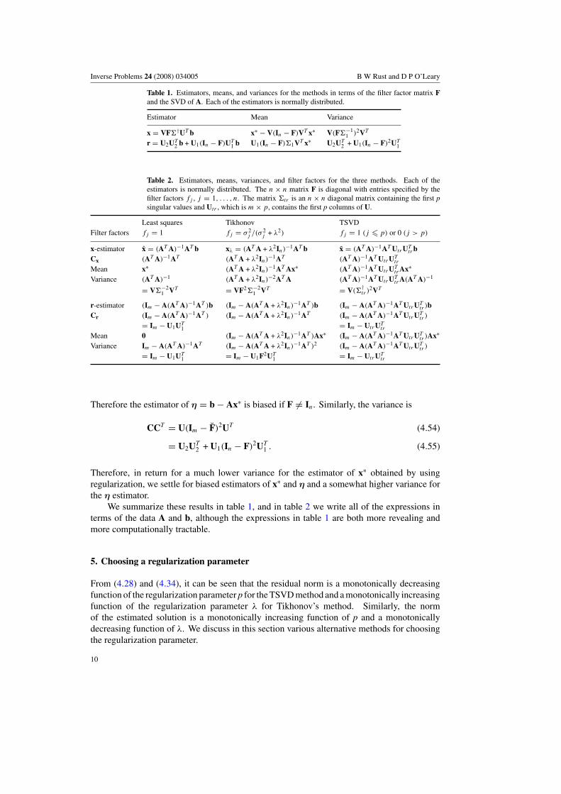
Table 1. Estimators, means, and variances for the methods in terms of the filter factor matrix Fand the SVD of A. Each of the estimators is normally distributed.

Estimator Mean Variance

x = VF�†UT b x∗ − V(In − F)VT x∗ V(F�−11 )2VT

r = U2UT2 b + U1(In − F)UT

1 b U1(In − F)�1VT x∗ U2UT2 + U1(In − F)2UT

1

Table 2. Estimators, means, variances, and filter factors for the three methods. Each of theestimators is normally distributed. The n × n matrix F is diagonal with entries specified by thefilter factors fj , j = 1, . . . , n. The matrix �tr is an n × n diagonal matrix containing the first psingular values and Utr , which is m × p, contains the first p columns of U.

Least squares Tikhonov TSVDFilter factors fj = 1 fj = σ 2

j /(σ 2j + λ2) fj = 1 (j � p) or 0 (j > p)

x-estimator x̂ = (AT A)−1AT b xλ = (AT A + λ2In)−1AT b x̃ = (AT A)−1AT UtrUT

trbCx (AT A)−1AT (AT A + λ2In)

−1AT (AT A)−1AT UtrUTtr

Mean x∗ (AT A + λ2In)−1AT Ax∗ (AT A)−1AT UtrUT

trAx∗

Variance (AT A)−1 (AT A + λ2In)−2AT A (AT A)−1AT UtrUT

trA(AT A)−1

= V�−21 VT = VF2�−2

1 VT = V(�†tr )

2VT

r-estimator (Im − A(AT A)−1AT )b (Im − A(AT A + λ2In)−1AT )b (Im − A(AT A)−1AT UtrUT

tr )bCr (Im − A(AT A)−1AT ) (Im − A(AT A + λ2In)

−1AT (Im − A(AT A)−1AT UtrUTtr )

= Im − U1UT1 = Im − UtrUT

tr

Mean 0 (Im − A(AT A + λ2In)−1AT )Ax∗ (Im − A(AT A)−1AT UtrUT

tr )Ax∗

Variance Im − A(AT A)−1AT (Im − A(AT A + λ2In)−1AT )2 (Im − A(AT A)−1AT UtrUT

tr )

= Im − U1UT1 = Im − U1F2UT

1 = Im − UtrUTtr

Therefore the estimator of η = b − Ax∗ is biased if F �= In. Similarly, the variance is

CCT = U(Im − F̆)2UT (4.54)

= U2UT2 + U1(In − F)2UT

1 . (4.55)

Therefore, in return for a much lower variance for the estimator of x∗ obtained by usingregularization, we settle for biased estimators of x∗ and η and a somewhat higher variance forthe η estimator.

We summarize these results in table 1, and in table 2 we write all of the expressions interms of the data A and b, although the expressions in table 1 are both more revealing andmore computationally tractable.

5. Choosing a regularization parameter

From (4.28) and (4.34), it can be seen that the residual norm is a monotonically decreasingfunction of the regularization parameter p for the TSVD method and a monotonically increasingfunction of the regularization parameter λ for Tikhonov’s method. Similarly, the normof the estimated solution is a monotonically increasing function of p and a monotonicallydecreasing function of λ. We discuss in this section various alternative methods for choosingthe regularization parameter.

10


5.1. Well-known methods

There are three common methods for choosing the regularization parameter.The most basic choice of regularization parameter is via Morozov’s discrepancy principle

[22]. This method chooses the regularization parameter so that the norm of the residual isapproximately equal to its expected value, given in (2.10).

An alternate strategy for Tikhonov regularization is to choose λ to minimize thegeneralized cross-validation (GCV) function

G(λ) =m∑

k=1

[bk − (Ax̃(k)

λ

)k

]2, (5.56)

where x̃(k)λ is the estimate when the kth measurement bk is omitted. The basic idea, first

introduced by Wahba [34], is to choose λ to make Ax̃λ the best overall predictor for missingdata values. The formulation for TSVD is similar, but in this case G(p) is a discrete functionrather than a continuous one.

A third strategy, often used when the error cannot be assumed to be normally distributed,is based on the L-curve first introduced by Hanson and Lawson [19] and further developed byHansen [9] and [11, chapter 4]. In current use, the L-curve for Tikhonov regularization is a plotof log ‖x̃λ‖ versus log ‖b − Ax̃λ‖ for a range of positive values of λ. The graph on the left offigure 5 is an L-curve plot for the modified Phillips problem. The λ chosen corresponds to thepoint in the corner where the curvature of the curve is maximized. A method for calculatingthis point has been described by Hansen and O’Leary [13], and Hansen [10] provides MATLAB

software for doing the calculations. The L-curve for TSVD is defined in a similar way, butconsists of discrete points for various values of p; curvature can be defined as the curvature ofa smoothing cubic spline.

5.2. Diagnostics based on statistical properties of the residual and its periodogram

Rust [25] (see also [26]) suggested several diagnostics for judging the acceptability of aregularized solution x̃ with residual r̃ using properties of the true residual η = r∗.

Diagnostic 1. The residual norm-squared should be within two standard deviations of theexpected value of ‖η‖2, which is m; in other words, ‖r̃‖2 ∈ [m − 2

√2m,m + 2

√2m]. This is

a way to quantify the Morozov discrepancy principle.

Diagnostic 2. The elements of η are drawn from a N(0, 1) distribution, and a graph of theelements of r̃ should look like samples from this distribution. (In fact, a histogram of theentries of r̃ should look like a bell curve.)

Diagnostic 3. We consider the elements of both η and r̃ as time series, with the index i(i = 1, . . . , m) taken to be the time variable. Since η ∼ N(0, Im), the ηi form a white noiseseries. Therefore the residuals r̃ for an acceptable estimate should constitute a realization ofsuch a series.

A formal test of diagnostics 2 and 3, used by Rust [25], is based on a plot of theperiodogram [5, chapter 7], which is an estimate of the power spectrum on the frequencyinterval 0 � f � 1

2T, where T is the sample spacing for the time variable. Here, the time

variable is the element number i, so T = 1. The periodogram is formed by zero-padding thetime series to a convenient length N (e.g., a power of 2), taking the discrete Fourier transformof this zero-padded series, and taking the squares of the absolute values of the first half ofthe coefficients. This gives us the periodogram z of values corresponding to the frequencies

11


k/NT , k = 0, . . . , N/2. The cumulative periodogram c is the vector of partial sums of theperiodogram, normalized by the sum of all of the elements; i.e.,

ck =∑k

j=0 zj∑N/2j=0 zj

, (5.57)

where z and c are vectors with (N + 1) components. The variance in a white noise recordis distributed uniformly on the interval 0 � f � 1

2T.5 Of course, no real noise record could

have such an even distribution of variance, but on average over many samples, the distributionwould approach that uniformity, and in the limit the periodogram would be flat. This meansthat a plot of the elements of c versus their frequencies fk = k/NT would be a straight linepassing through the origin with slope 2/NT . Since the Fourier transform of the residuals isobtained by a linear transformation with an orthogonal matrix, the real and imaginary partsof the transform would remain independently, normally distributed. This implies that theperiodogram ordinates would be multiples of independent χ2(2) samples and hence that theck would be distributed like an ordered sample of size N/2 from a uniform (0,1) distribution.A test of the hypothesis that the residuals are white noise can be obtained by constructing thetwo lines parallel to the one above, passing through the points (f, c) = (0,±δ), where δ is the5% point for the Kolomogorov–Smirnov statistics for a sample of size m/2. These two linesdefine a 95% confidence band for white noise. More details on this procedure can be found inFuller [5, pp 363–6].

Therefore, the ideal cumulative periodogram is a straight line between 0 and 1 as thefrequency varies between 0 and 0.5, so we expect its length to be close to 1.118 (takingT = 1). Quantitative measures for diagnostics 2 and 3 can be based on the length of thecumulative periodogram (estimated as the length of the piecewise linear interpolant to thecumulative periodogram) and on the number of samples outside the 95% confidence band.These measures, along with the residual norm-squared for diagnostic 1, comprise our numericaldiagnostics, which we use in conjunction with the plots of the residual vector, its periodogramand its cumulative periodogram.

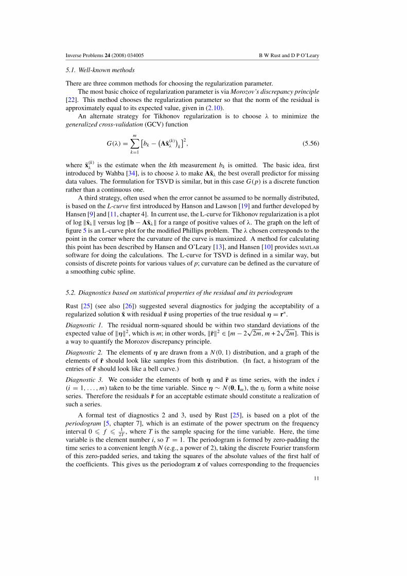
As an example, we apply these diagnostics to the linear regression estimate x̂ (see(3.13)) for the modified Phillips problem discussed in section 3. Using these diagnostics,we see that this estimate of the solution is not reasonable. We have already observed that‖r̂‖2 = 43.01, which is outside the ±2σ confidence interval [251.02, 348.98], so diagnostic1 is violated. The components of the residual r̂ are plotted against i in the middle left infigure 2, with their histogram displayed in the bottom left. They do not look like samples froma N(0, 1) distribution, so diagnostic 2 is violated. By considering plots of the periodogramand cumulative periodogram on the right in the figure, we see that diagnostic 3 is violated.The middle-right graph in figure 2 is a plot of a periodogram estimate at 4097 equally spacedfrequency points on the interval [0, 0.5]. For white noise, the variance would be distributeduniformly, but there is much more power on [0, 0.25] than on [0.25, 0.5] so the residuals areprobably not white noise. The cumulative periodogram is the solid curve at the bottom rightof figure 2. The title gives the length of this curve, which can be compared with the value1.11803 expected for pure white noise. The dashed lines enclose a 95% confidence band forwhite noise. We expect that the ordinates for a white noise series should lie outside this bandfor at most 5% of the frequencies. Since 2803 of the 4096 lie outside the band, it is clear thatthe least squares residuals are not white noise. Thus, the linear regression estimate fails allthree diagnostics and is not an acceptable solution. For comparison, the true solution x∗ withresidual η passes all three diagnostics, as illustrated in figure 4.5 This interval defines the Nyquist band, and the power spectrum for white noise is constant at all frequencies in thisband, since the autocorrelation function for white noise is zero for all lags except lag 0.

12


Figure 4. True solution (top) and diagnostics for the modified Phillips problem. On the leftare the residual and its histogram. On the right are the residual periodogram and the cumulativeperiodogram.

In [25], Rust suggested choosing a parameter that passed all three of the diagnostics givenabove. Later Hansen, Kilmer and Kjeldsen [12] proposed choosing the parameter by either oftwo methods.

• Choosing the most regularized solution estimate for which the cumulative periodogramlies within the 95% confidence interval.

• Minimizing the sum of the absolute values of the difference between components of cand the straight line passing through the origin with slope 2/NT .

The first method tends to undersmooth, since we would expect 5% of the samples to lieoutside the confidence interval. For similar reasons, the second method is also too stringent.

13


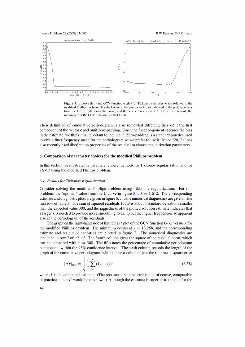
Figure 5. L-curve (left) and GCV function (right) for Tikhonov estimates to the solution to themodified Phillips problem. For the L-Curve, the parameter λ (not indicated in the plot) increasesfrom the left to right along the curve, and the ‘corner’ occurs at λ ≈ 1.612. In contrast, theminimizer for the GCV function is λ ≈ 13.268.

Their definition of cumulative periodogram is also somewhat different; they omit the firstcomponent of the vector c and omit zero-padding. Since the first component captures the biasin the estimate, we think it is important to include it. Zero-padding is a standard practice usedto give a finer frequency mesh for the periodogram so we prefer to use it. Mead [20, 21] hasalso recently used distribution properties of the residual to choose regularization parameters.

6. Comparison of parameter choices for the modified Phillips problem

In this section we illustrate the parameter choice methods for Tikhonov regularization and forTSVD using the modified Phillips problem.

6.1. Results for Tikhonov regularization

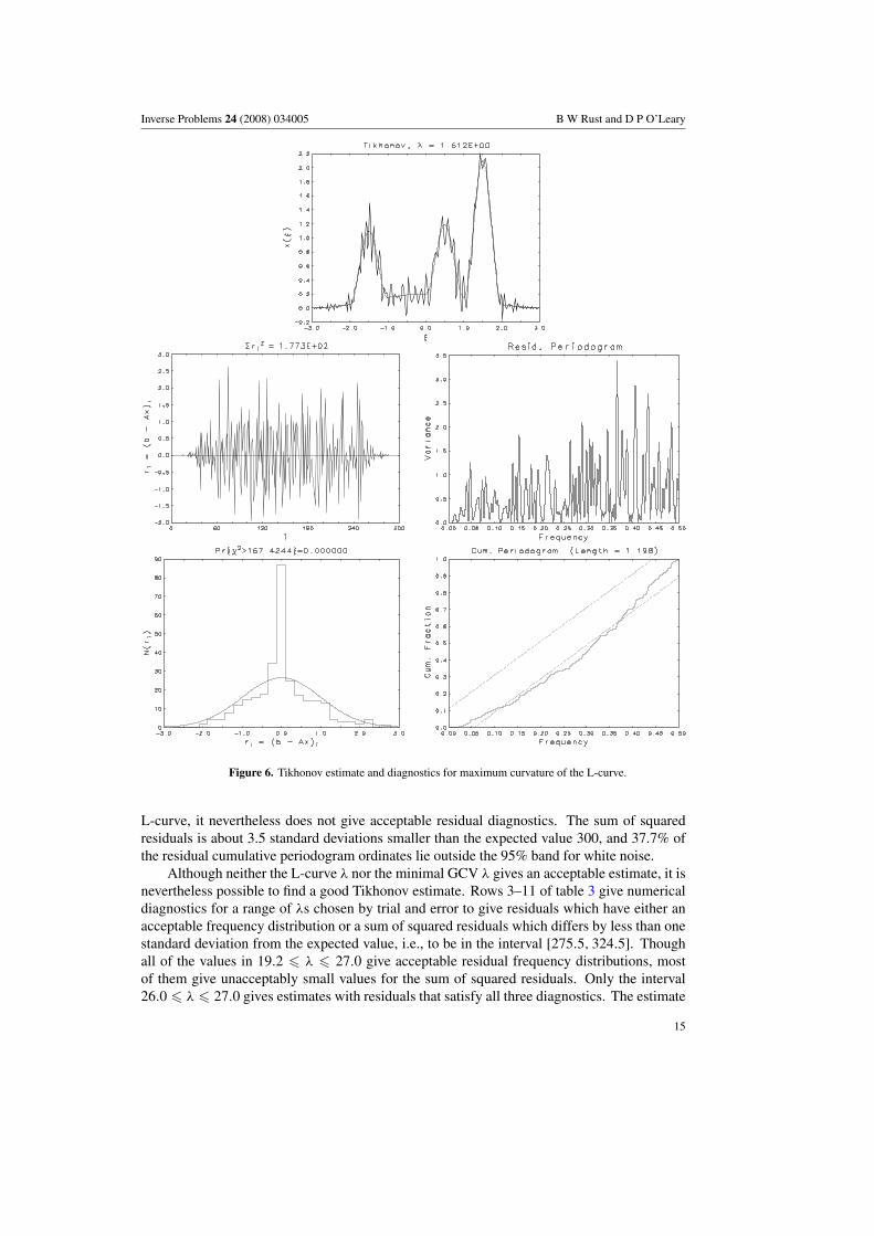
Consider solving the modified Phillips problem using Tikhonov regularization. For thisproblem, the ‘optimal’ value from the L-curve in figure 5 is λ = 1.612. The correspondingestimate and diagnostic plots are given in figure 6, and the numerical diagnostics are given in thefirst row of table 3. The sum of squared residuals 177.3 is about 5 standard deviations smallerthan the expected value 300, and the jaggedness of the plotted solution estimate indicates thata larger λ is needed to provide more smoothing to damp out the higher frequencies so apparentalso in the periodogram of the residuals.

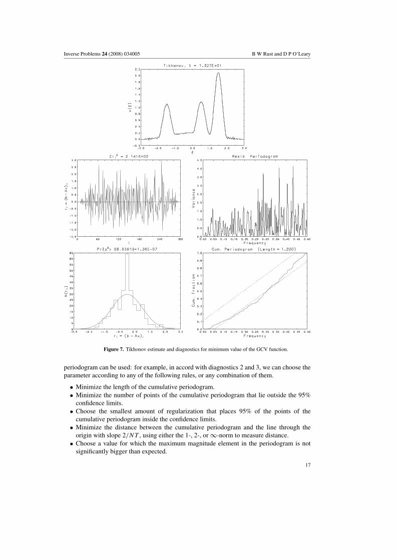
The graph on the right-hand side of figure 5 is a plot of the GCV function G(λ) versus λ forthe modified Phillips problem. The minimum occurs at λ = 13.268, and the correspondingestimate and residual diagnostics are plotted in figure 7. The numerical diagnostics aretabulated in row 2 of table 3. The fourth column gives the square of the residual norm, whichcan be compared with m = 300. The fifth notes the percentage of cumulative periodogramcomponents within the 95% confidence interval. The sixth column records the length of thegraph of the cumulative periodogram, while the next column gives the root mean square error

|x|rms ≡√√√√1

n

n∑j=1

(x̃j − x∗j )2, (6.58)

where x̃ is the computed estimate. (The root-mean-square error is not, of course, computablein practice, since x∗ would be unknown.) Although the estimate is superior to the one for the

14


Figure 6. Tikhonov estimate and diagnostics for maximum curvature of the L-curve.

L-curve, it nevertheless does not give acceptable residual diagnostics. The sum of squaredresiduals is about 3.5 standard deviations smaller than the expected value 300, and 37.7% ofthe residual cumulative periodogram ordinates lie outside the 95% band for white noise.

Although neither the L-curve λ nor the minimal GCV λ gives an acceptable estimate, it isnevertheless possible to find a good Tikhonov estimate. Rows 3–11 of table 3 give numericaldiagnostics for a range of λs chosen by trial and error to give residuals which have either anacceptable frequency distribution or a sum of squared residuals which differs by less than onestandard deviation from the expected value, i.e., to be in the interval [275.5, 324.5]. Thoughall of the values in 19.2 � λ � 27.0 give acceptable residual frequency distributions, mostof them give unacceptably small values for the sum of squared residuals. Only the interval26.0 � λ � 27.0 gives estimates with residuals that satisfy all three diagnostics. The estimate

15


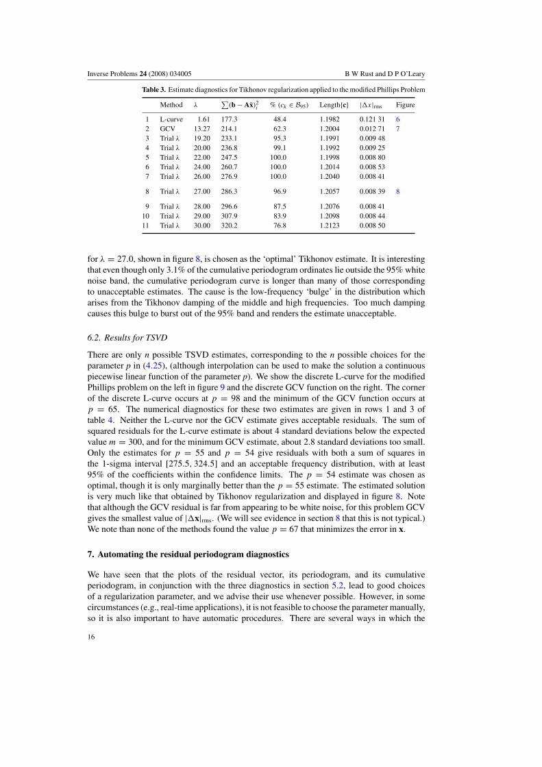
Table 3. Estimate diagnostics for Tikhonov regularization applied to the modified Phillips Problem

Method λ∑

(b − Ax̃)2i % (ck ∈ B95) Length{c} |x|rms Figure

1 L-curve 1.61 177.3 48.4 1.1982 0.121 31 62 GCV 13.27 214.1 62.3 1.2004 0.012 71 73 Trial λ 19.20 233.1 95.3 1.1991 0.009 484 Trial λ 20.00 236.8 99.1 1.1992 0.009 255 Trial λ 22.00 247.5 100.0 1.1998 0.008 806 Trial λ 24.00 260.7 100.0 1.2014 0.008 537 Trial λ 26.00 276.9 100.0 1.2040 0.008 41

8 Trial λ 27.00 286.3 96.9 1.2057 0.008 39 8

9 Trial λ 28.00 296.6 87.5 1.2076 0.008 4110 Trial λ 29.00 307.9 83.9 1.2098 0.008 4411 Trial λ 30.00 320.2 76.8 1.2123 0.008 50

for λ = 27.0, shown in figure 8, is chosen as the ‘optimal’ Tikhonov estimate. It is interestingthat even though only 3.1% of the cumulative periodogram ordinates lie outside the 95% whitenoise band, the cumulative periodogram curve is longer than many of those correspondingto unacceptable estimates. The cause is the low-frequency ‘bulge’ in the distribution whicharises from the Tikhonov damping of the middle and high frequencies. Too much dampingcauses this bulge to burst out of the 95% band and renders the estimate unacceptable.

6.2. Results for TSVD

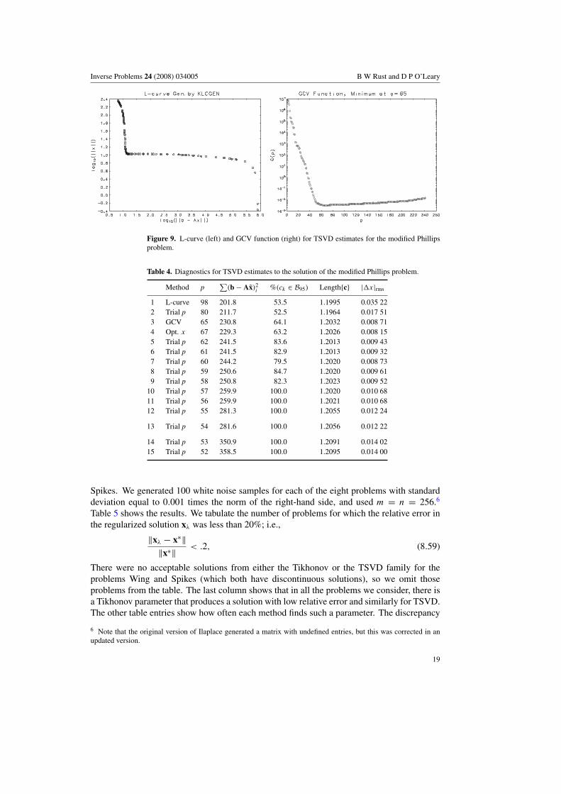
There are only n possible TSVD estimates, corresponding to the n possible choices for theparameter p in (4.25), (although interpolation can be used to make the solution a continuouspiecewise linear function of the parameter p). We show the discrete L-curve for the modifiedPhillips problem on the left in figure 9 and the discrete GCV function on the right. The cornerof the discrete L-curve occurs at p = 98 and the minimum of the GCV function occurs atp = 65. The numerical diagnostics for these two estimates are given in rows 1 and 3 oftable 4. Neither the L-curve nor the GCV estimate gives acceptable residuals. The sum ofsquared residuals for the L-curve estimate is about 4 standard deviations below the expectedvalue m = 300, and for the minimum GCV estimate, about 2.8 standard deviations too small.Only the estimates for p = 55 and p = 54 give residuals with both a sum of squares inthe 1-sigma interval [275.5, 324.5] and an acceptable frequency distribution, with at least95% of the coefficients within the confidence limits. The p = 54 estimate was chosen asoptimal, though it is only marginally better than the p = 55 estimate. The estimated solutionis very much like that obtained by Tikhonov regularization and displayed in figure 8. Notethat although the GCV residual is far from appearing to be white noise, for this problem GCVgives the smallest value of |x|rms. (We will see evidence in section 8 that this is not typical.)We note than none of the methods found the value p = 67 that minimizes the error in x.

7. Automating the residual periodogram diagnostics

We have seen that the plots of the residual vector, its periodogram, and its cumulativeperiodogram, in conjunction with the three diagnostics in section 5.2, lead to good choicesof a regularization parameter, and we advise their use whenever possible. However, in somecircumstances (e.g., real-time applications), it is not feasible to choose the parameter manually,so it is also important to have automatic procedures. There are several ways in which the

16


Figure 7. Tikhonov estimate and diagnostics for minimum value of the GCV function.

periodogram can be used: for example, in accord with diagnostics 2 and 3, we can choose theparameter according to any of the following rules, or any combination of them.

• Minimize the length of the cumulative periodogram.• Minimize the number of points of the cumulative periodogram that lie outside the 95%

confidence limits.• Choose the smallest amount of regularization that places 95% of the points of the

cumulative periodogram inside the confidence limits.• Minimize the distance between the cumulative periodogram and the line through the

origin with slope 2/NT , using either the 1-, 2-, or ∞-norm to measure distance.• Choose a value for which the maximum magnitude element in the periodogram is not

significantly bigger than expected.

17


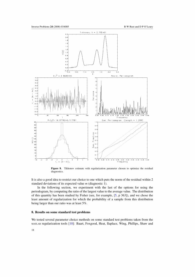
Figure 8. Tikhonov estimate with regularization parameter chosen to optimize the residualdiagnostics.

It is also a good idea to restrict our choice to one which puts the norm of the residual within 2standard deviations of its expected value m (diagnostic 1).

In the following section, we experiment with the last of the options for using theperiodogram, by computing the ratio of the largest value to the average value. The distributionof this quantity has been studied by Fisher (see, for example, [5, p 363]), and we chose theleast amount of regularization for which the probability of a sample from this distributionbeing larger than our ratio was at least 5%.

8. Results on some standard test problems

We tested several parameter choice methods on some standard test problems taken from theMATLAB regularization tools [10]: Baart, Foxgood, Heat, Ilaplace, Wing, Phillips, Shaw and

18


Figure 9. L-curve (left) and GCV function (right) for TSVD estimates for the modified Phillipsproblem.

Table 4. Diagnostics for TSVD estimates to the solution of the modified Phillips problem.

Method p∑

(b − Ax̃)2i %(ck ∈ B95) Length{c} |x|rms

1 L-curve 98 201.8 53.5 1.1995 0.035 222 Trial p 80 211.7 52.5 1.1964 0.017 513 GCV 65 230.8 64.1 1.2032 0.008 714 Opt. x 67 229.3 63.2 1.2026 0.008 155 Trial p 62 241.5 83.6 1.2013 0.009 436 Trial p 61 241.5 82.9 1.2013 0.009 327 Trial p 60 244.2 79.5 1.2020 0.008 738 Trial p 59 250.6 84.7 1.2020 0.009 619 Trial p 58 250.8 82.3 1.2023 0.009 52

10 Trial p 57 259.9 100.0 1.2020 0.010 6811 Trial p 56 259.9 100.0 1.2021 0.010 6812 Trial p 55 281.3 100.0 1.2055 0.012 24

13 Trial p 54 281.6 100.0 1.2056 0.012 22

14 Trial p 53 350.9 100.0 1.2091 0.014 0215 Trial p 52 358.5 100.0 1.2095 0.014 00

Spikes. We generated 100 white noise samples for each of the eight problems with standarddeviation equal to 0.001 times the norm of the right-hand side, and used m = n = 256.6

Table 5 shows the results. We tabulate the number of problems for which the relative error inthe regularized solution xλ was less than 20%; i.e.,

‖xλ − x∗‖‖x∗‖ < .2, (8.59)

There were no acceptable solutions from either the Tikhonov or the TSVD family for theproblems Wing and Spikes (which both have discontinuous solutions), so we omit thoseproblems from the table. The last column shows that in all the problems we consider, there isa Tikhonov parameter that produces a solution with low relative error and similarly for TSVD.The other table entries show how often each method finds such a parameter. The discrepancy

6 Note that the original version of Ilaplace generated a matrix with undefined entries, but this was corrected in anupdated version.

19


Table 5. Number of solutions with relative error less than 20%.

Problem Method PFT Discr. GCV L-Curve HKK Optimal

Bart Tikhonov 96 59 67 75 98 100TSVD 93 58 70 37 97 100

Foxgood Tikhonov 98 58 81 76 99 100TSVD 96 58 79 35 99 100

Heat Tikhonov 91 84 86 4 99 100TSVD 67 62 86 21 35 100

Ilaplace Tikhonov 95 68 81 88 99 100TSVD 96 68 81 78 99 100

Phillips Tikhonov 100 91 100 87 100 100TSVD 99 89 96 37 97 100

Shaw Tikhonov 99 59 80 79 99 100TSVD 96 60 88 69 98 100

Overall Tikhonov 579 419 495 409 594 600(97%) (70%) (83%) (68%) (99%) (100%)

TSVD 547 395 500 277 525 600(91%) (66%) (83%) (46%) (88%) (100%)

principle (Discr.), which chooses the parameter for which the residual norm is closest to itsexpected value, is a rather reliable method, producing a solution with low relative error forTikhonov on 70% of the examples and for TSVD on 66% of the examples. The GCV workseven better, with an acceptable solution in 83% of the examples, despite the fact that the GCVfunction is notorious for being flat, making it difficult to find a minimizer. The L-curve isslightly less reliable than the discrepancy principle, but still works well in about 68% of theproblems for Tikhonov and 46% for TSVD. Often it fails due to a bad estimate of the locationof the corner, since it is easily fooled by roughness in the curve. The periodogram with Fishertest (PFT) is quite reliable, finding an acceptable solution for 97% of the problems whenusing the Tikhonov method and 91% when using TSVD. This is comparable to the resultsfor the method of Hansen, Kilmer and Kjeldsen (HKK), but their method has the statisticalflaws of ignoring the first component of the periodogram and of demanding that 100% ofthe cumulative periodogram values lie within a 95% confidence interval. Based on these andother tests, we conclude that many variants of parameter choice methods based on residualperiodograms are quite effective.

9. A real-world example

In the previous section we demonstrated the effectiveness of using the Fisher test on theperiodogram in order to automatically determine a regularization parameter. In this sectionwe demonstrate how a spectroscopy problem can be solved using manual application of thediagnostics.

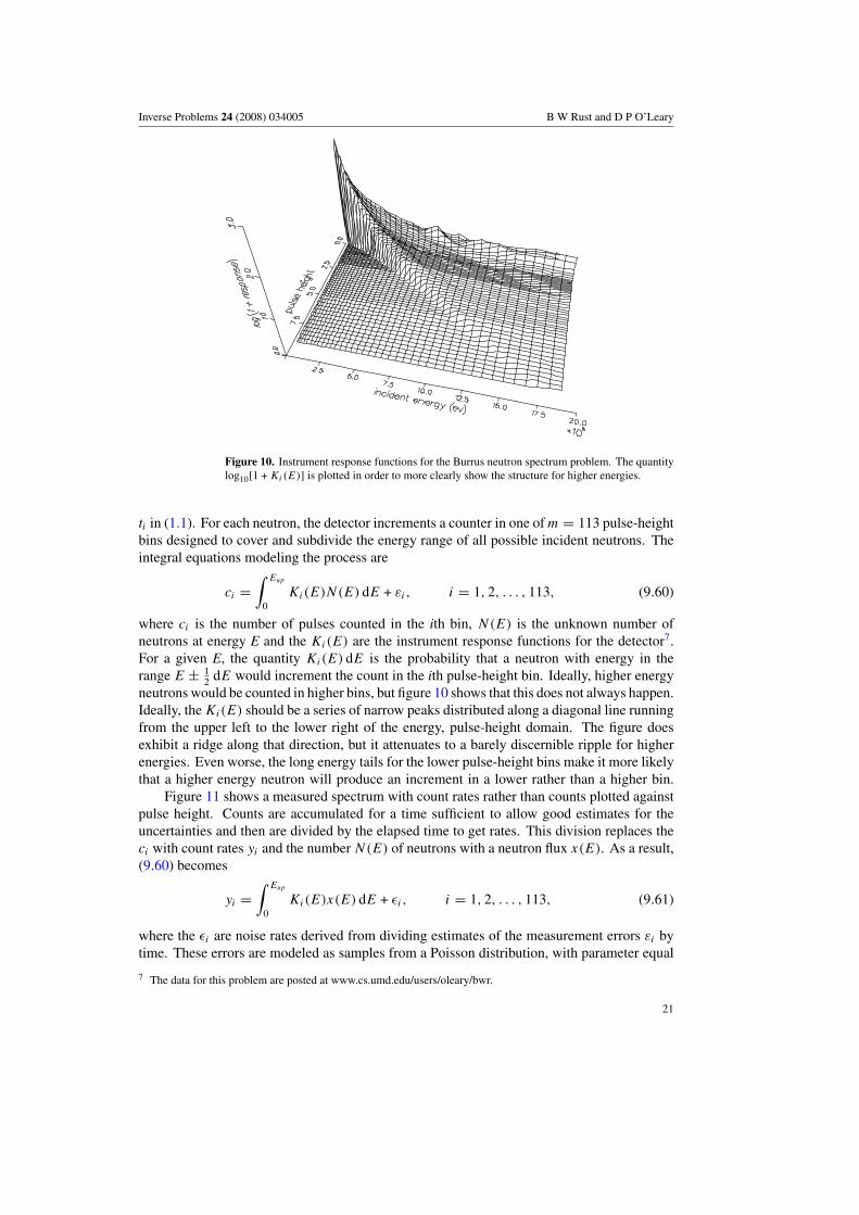
Measurements of nuclear radiation spectra are an important source of ill-posed problems.Consider the energy spectrum of neutrons produced by the reaction T (d, n)4He, i.e. tritiumnuclei bombarded with deuterons to produce helium nuclei and the neutrons being measured.If the bombarding particles are monoenergetic then so are the neutrons produced. Although theneutrons are monoenergetic, the measuring instrument both smears and distorts the expectedspectrum. The instrument in question, an NE-213 spectrometer, has been described byVerbinski et al [33] and Burrus and Verbinski [3]. Its response functions are plotted infigure 10, where incident energy corresponds to the variable ξ and pulse height to the variable

20


Figure 10. Instrument response functions for the Burrus neutron spectrum problem. The quantitylog10[1 + Ki(E)] is plotted in order to more clearly show the structure for higher energies.

ti in (1.1). For each neutron, the detector increments a counter in one of m = 113 pulse-heightbins designed to cover and subdivide the energy range of all possible incident neutrons. Theintegral equations modeling the process are

ci =∫ Eup

0Ki(E)N(E) dE + εi, i = 1, 2, . . . , 113, (9.60)

where ci is the number of pulses counted in the ith bin, N(E) is the unknown number ofneutrons at energy E and the Ki(E) are the instrument response functions for the detector7.For a given E, the quantity Ki(E) dE is the probability that a neutron with energy in therange E ± 1

2 dE would increment the count in the ith pulse-height bin. Ideally, higher energyneutrons would be counted in higher bins, but figure 10 shows that this does not always happen.Ideally, the Ki(E) should be a series of narrow peaks distributed along a diagonal line runningfrom the upper left to the lower right of the energy, pulse-height domain. The figure doesexhibit a ridge along that direction, but it attenuates to a barely discernible ripple for higherenergies. Even worse, the long energy tails for the lower pulse-height bins make it more likelythat a higher energy neutron will produce an increment in a lower rather than a higher bin.

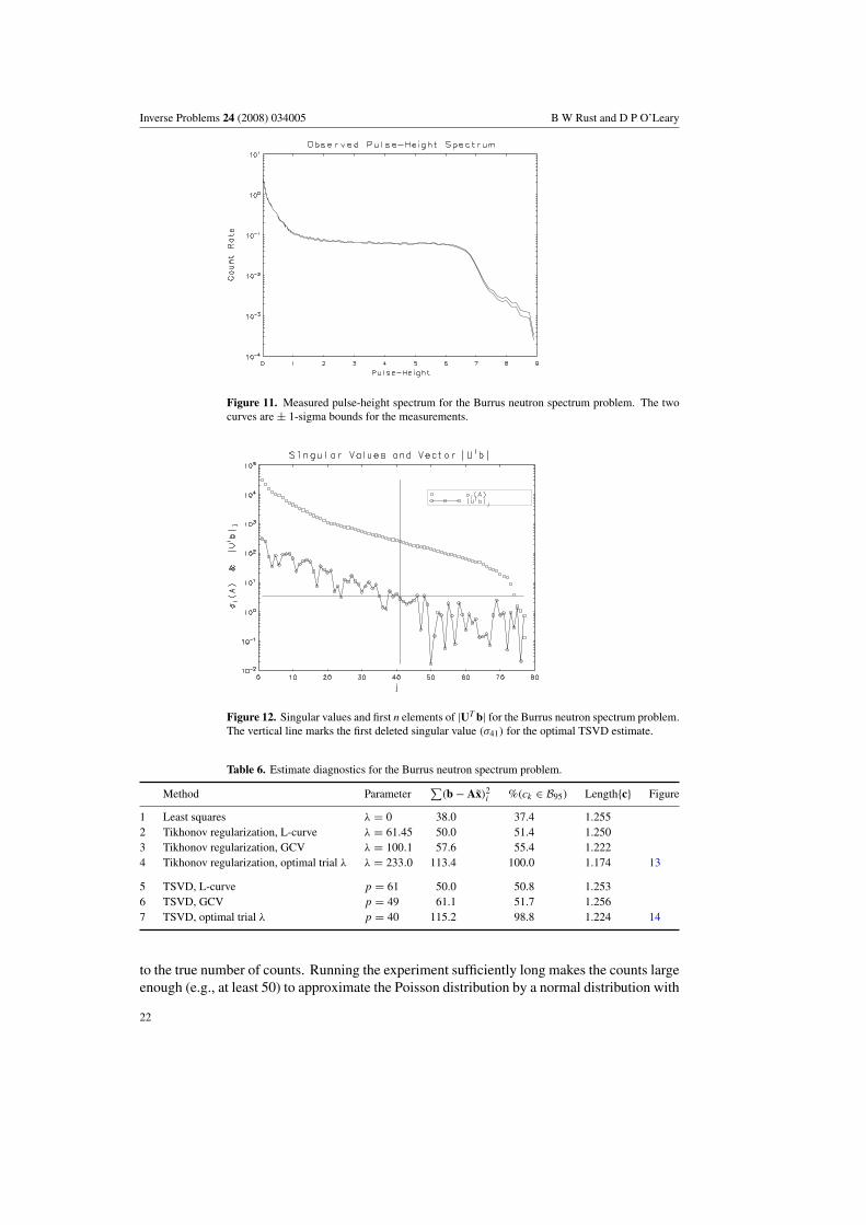
Figure 11 shows a measured spectrum with count rates rather than counts plotted againstpulse height. Counts are accumulated for a time sufficient to allow good estimates for theuncertainties and then are divided by the elapsed time to get rates. This division replaces theci with count rates yi and the number N(E) of neutrons with a neutron flux x(E). As a result,(9.60) becomes

yi =∫ Eup

0Ki(E)x(E) dE + εi, i = 1, 2, . . . , 113, (9.61)

where the εi are noise rates derived from dividing estimates of the measurement errors εi bytime. These errors are modeled as samples from a Poisson distribution, with parameter equal

7 The data for this problem are posted at www.cs.umd.edu/users/oleary/bwr.

21


Figure 11. Measured pulse-height spectrum for the Burrus neutron spectrum problem. The twocurves are ± 1-sigma bounds for the measurements.

Figure 12. Singular values and first n elements of |UT b| for the Burrus neutron spectrum problem.The vertical line marks the first deleted singular value (σ41) for the optimal TSVD estimate.

Table 6. Estimate diagnostics for the Burrus neutron spectrum problem.

Method Parameter∑

(b − Ax̃)2i %(ck ∈ B95) Length{c} Figure

1 Least squares λ = 0 38.0 37.4 1.2552 Tikhonov regularization, L-curve λ = 61.45 50.0 51.4 1.2503 Tikhonov regularization, GCV λ = 100.1 57.6 55.4 1.2224 Tikhonov regularization, optimal trial λ λ = 233.0 113.4 100.0 1.174 13

5 TSVD, L-curve p = 61 50.0 50.8 1.2536 TSVD, GCV p = 49 61.1 51.7 1.2567 TSVD, optimal trial λ p = 40 115.2 98.8 1.224 14

to the true number of counts. Running the experiment sufficiently long makes the counts largeenough (e.g., at least 50) to approximate the Poisson distribution by a normal distribution with

22


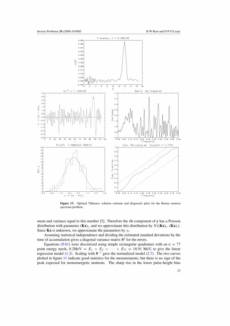
Figure 13. Optimal Tikhonov solution estimate and diagnostic plots for the Burrus neutronspectrum problem.

mean and variance equal to this number [5]. Therefore the ith component of y has a Poissondistribution with parameter (Kx)i , and we approximate this distribution by N((Kx)i, (Kx)i).Since Kx is unknown, we approximate the parameters by yi .

Assuming statistical independence and dividing the estimated standard deviations by thetime of accumulation gives a diagonal variance matrix S2 for the errors.

Equations (9.61) were discretized using simple rectangular quadrature with an n = 77point energy mesh, 0.2MeV = E1 < E2 < · · · < E77 = 18.91 MeV, to give the linearregression model (1.2). Scaling with S−1 gave the normalized model (2.7). The two curvesplotted in figure 11 indicate good statistics for the measurements, but there is no sign of thepeak expected for monoenergetic neutrons. The sharp rise in the lower pulse-height bins

23


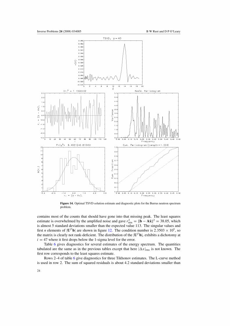
Figure 14. Optimal TSVD solution estimate and diagnostic plots for the Burrus neutron spectrumproblem.

contains most of the counts that should have gone into that missing peak. The least squaresestimate is overwhelmed by the amplified noise and gave r2

min = ‖b − Ax̂‖2 = 38.05, whichis almost 5 standard deviations smaller than the expected value 113. The singular values andfirst n elements of |UT b| are shown in figure 12. The condition number is 2.3503 × 105, sothe matrix is clearly not rank-deficient. The distribution of the |UT b|i exhibits a dichotomy ati = 47 where it first drops below the 1-sigma level for the error.

Table 6 gives diagnostics for several estimates of the energy spectrum. The quantitiestabulated are the same as in the previous tables except that here |x|rms is not known. Thefirst row corresponds to the least squares estimate.

Rows 2–4 of table 6 give diagnostics for three Tikhonov estimates. The L-curve methodis used in row 2. The sum of squared residuals is about 4.2 standard deviations smaller than

24


the expected value, and an excess of higher frequencies rendered the frequency distributionof the residuals unacceptable. In row 3, the smoothing constant is chosen to minimize theGCV function. The sum of squared residuals is about 3.7 standard deviations smaller thanthe expected value, and the frequency distribution of the residuals is unacceptable. For theestimate in row 4, the smoothing constant is chosen by trial and error to give a sum of squaredresiduals close to the expected value 113. The estimated solution and diagnostic plots aregiven in figure 13.

Rows 5–7 of table 6 give diagnostics for three estimates obtained from the TSVDmethod. For rows 5 and 6, the truncation parameters are chosen by the L-curve and minimumGCV methods, respectively. The estimate and diagnostics are very similar to those for thecorresponding Tikhonov estimates (rows 1 and 2): the estimated solution is reasonable but theresidual is unacceptable. Row 7 gives the diagnostics for the optimal TSVD truncation. Thesolution estimate and diagnostic plots are given in figure 14.

10. Discussion and conclusions

For ill-posed problems with errors dominated by the measurement uncertainties in y, theinstability in the solution estimate is attributable to components of the measurements whichare overwhelmed by those uncertainties. In general, these components do not correspondexactly to specific elements of y. When possible, we advocate scaling the problem by S−1 totransform it to one in which the errors all have unit variance. Regularization methods can thenbe used to reduce the influence of the error. Ideally, the results of candidate parameter choicesshould be evaluated by plotting the resulting residual along with its periodogram and itscumulative periodogram and examining the numerical diagnostics. Sometimes an automatedchoice is needed, and in such cases we advise using diagnostics based on the norm of theresidual and the periodogram of the residual to choose or validate the choice of a regularizationparameter.

To apply either the manual or the automatic methods for parameter choice, one need onlybe able to compute the Fourier coefficients of the (zero-padded) residual for various valuesof the regularization parameter. Thus all of these numerical diagnostics are inexpensive tocompute, so they can be used for two- and three-dimensional problems, even if regularizationmethods other than the SVD-based ones discussed here are used. They can be used, forexample, in conjunction with iterative regularization methods [18] or even with nonlinearmodels.

Of course, there is no guarantee that the estimate resulting from our parameter choicemethod will be close to the true solution, since (quite likely) the assumption that the errors η

are N(0, Im) may only be an approximation. Even if the assumption is good, noise may belarge enough to overwhelm important components of the signal. To recover such componentsit is necessary to repeat the measurements multiple times or with more accuracy.

Acknowledgments

BWR would like to thank Drs W R Burrus and R E Funderlic for the initial inspiration. Wethank Drs A S Carasso, K J Coakley, D E Gilsinn, K A Remington, and the anonymousreferees for their reviews and suggestions and Dr M G Vangel for suggestions for improvingthe statistical aspects of this manuscript. We are grateful to Drs M E Kilmer and P C Hansenfor sharing their software. The work of the second author was supported in part by theNational Science Foundation under grant CCF 0514213. The views expressed here are those

25


of the authors alone, not necessarily those of NIST or NSF. Certain commercial productsare identified in order to specify adequately experimental procedures. In no case does suchidentification imply recommendation or endorsement by NIST, nor does it imply that the itemsidentified are necessarily the best available for the purpose.

Appendix A. A variant of the Phillips problem

A useful test problem which shares many of the characteristics of real instrument correctionproblems is obtained by discretizing a variant of the well-known [23] Phillips equation. Thismodified Phillips problem can be written as

y(t) =∫ 3

−3K(t, ξ)x(ξ) dξ, −6 � t � 6, (A.1)

with the kernel given by

K(t, ξ) =⎧⎨⎩

1

6

{1 + cos

[π3

(ξ − t)]}

, |ξ − t | � 3, |t | � 6,

0, otherwise,(A.2)

and the exact solution by

x(ξ) = β(ξ) +3∑

k=1

ck(ξ), (A.3)

where

β(ξ) =⎧⎨⎩α0

[1 + cos

(π

3ξ)]

, |ξ | � 3,

0, |ξ | > 3,

(A.4)

and

ck(ξ) ={

αk{1 + cos[2π(ξ − ψk)]}, |ξ − ψk| � 12 ,

0, otherwise,(A.5)

with amplitude constants αk and centering constants ψk chosen to be

α0 = 0.1, α1 = 0.5, α2 = 0.5, α3 = 1.0,

ψ1 = −1.5, ψ2 = 0.5, ψ3 = 1.5.(A.6)

The kernel differs from the Phillips original only in the inclusion of the normalizing factor 16

which is added to assure that for any ξ ,∫ 3+ξ

−3+ξ

K(t, ξ) dt = 1. (A.7)

For a measuring instrument this condition assures that conservation laws are not violated.Plots of K(t, ξ) for 5 representative values of ξ are given on the left in figure 1.

The exact solution to the original Phillips problem appears in a scaled down formas the β(ξ) term in the solution to the new problem. The scaling constant α0 is chosento reduce the original Phillips solution to the role of a background function on which tosuperimpose the three discrete peaks represented by the ck(ξ) terms. The three points ξ = ψk

are the centers of these peaks and the constants 2αk are their heights above the background.The new solution function is plotted as a dashed line on the right in figure 1.

26


These changes in the Phillips problem are designed to make it more challenging and morereminiscent of real-world instrument correction problems. Unfortunately, they also make therepresentation of the function y(t) more complicated. Substituting (A.3) into (A.1) gives

y(t) =∫ 3

−3K(t, ξ)β(ξ) dξ +

3∑k=1

∫ 3

−3K(t, ξ)ck(ξ) dξ, −6 � t � 6, (A.8)

but care must be exercised in evaluating these integrals because K(t, ξ) = 0 on half of therectangular domain {(t, ξ)|−6 � t � 6,−3 � ξ � 3} and each of the ck(ξ) is zero everywhereexcept on the interval ψk − 1

2 � ξ � ψk + 12 . The last equation can also be written as

y(t) = B(t) +3∑

k=1

Ck(t), (A.9)

where

B(t) ≡∫ 3

−3K(t, ξ)β(ξ) dξ, (A.10)

and

Ck(t) ≡∫ ψk+ 1

2

ψk− 12

K(t, ξ)ck(ξ) dξ, k = 1, 2, 3. (A.11)

Evaluating the integral for B(t) gives

B(t) = 1

6α0

{(6 − |t |)

[1 +

1

2cos(π

3t)]

+9

2πsin(π

3|t |)}

, −6 � t � 6, (A.12)

and the integrals for Ck(t) can be written as

Ck(t) = 16αkLk(t), k = 1, 2, 3, (A.13)

where

L1(t) =

⎧⎪⎪⎪⎪⎪⎪⎪⎪⎪⎪⎪⎪⎪⎪⎪⎪⎪⎪⎪⎪⎪⎪⎪⎨⎪⎪⎪⎪⎪⎪⎪⎪⎪⎪⎪⎪⎪⎪⎪⎪⎪⎪⎪⎪⎪⎪⎪⎩

0, −6 � t � −5,

t + 5 + 12π

sin[π(2t + 9)] + 3π

sin[

π3 (t + 2)

]+ 3

10π

{sin[π(2t + 8)] − sin

[π3 (t − 1)

]}+ 3

14π

{sin[π(2t + 10)] + sin

[π3 (t + 5)

]}, −5 � t � −4,

1 + 3π

{− sin[

π3 (1 + t)

]+ sin

[π3 (2 + t)

]}+ 3

10π

{sin[

π3 (4 + t)

]+ sin

[π3 (1 − t)

]}+ 3

14π

{sin[

π3 (2 − t)

]+ sin

[π3 (5 + t)

]}, −4 � t � 1,

2 − t + 12π

sin[π(3 − 2t)] − 3π

sin[

π3 (t + 1)

]+ 3

10π

{sin[

π3 (t + 4)

]+ sin [π(2 − 2t)]

}+ 3

14π

{sin[

π3 (2 − t)

]+ sin [π(4 − 2t)]

}, 1 � t � 2,

0, 2 � t � 6,

(A.14)

27


L2(t) =

⎧⎪⎪⎪⎪⎪⎪⎪⎪⎪⎪⎪⎪⎪⎪⎪⎪⎪⎪⎪⎪⎪⎪⎪⎨⎪⎪⎪⎪⎪⎪⎪⎪⎪⎪⎪⎪⎪⎪⎪⎪⎪⎪⎪⎪⎪⎪⎪⎩

0, −6 � t � −3,

t + 3 + 12π

sin[π(2t + 5)] + 3π

sin[

π3 t]

+ 310π

{sin[π(2t + 4)] − sin

[π3 (t − 3)

]}+ 3

14π

{sin[π(2t + 6)] + sin

[π3 (t + 3)

]}, −3 � t � −2,

1 + 3π

{sin[

π3 (1 − t)

]+ sin

[π3 t]}

+ 310π

{sin[

π3 (2 + t)

]+ sin

[π3 (3 − t)

]}+ 3

14π

{sin[

π3 (4 − t)

]+ sin

[π3 (3 + t)

]}, −2 � t � 3,

4 − t + 12π

sin[π(7 − 2t)] + 3π

sin[

π3 (1 − t)

]+ 3

10π

{sin[

π3 (t + 2)

]− sin [π(2t − 6)]}

+ 314π

{sin[

π3 (4 − t)

]− sin [π(2t − 8)]}, 3 � t � 4,

0, 4 � t � 6,

(A.15)

and

L3(t) =

⎧⎪⎪⎪⎪⎪⎪⎪⎪⎪⎪⎪⎪⎪⎪⎪⎪⎪⎪⎪⎪⎪⎪⎪⎨⎪⎪⎪⎪⎪⎪⎪⎪⎪⎪⎪⎪⎪⎪⎪⎪⎪⎪⎪⎪⎪⎪⎪⎩

0, −6 � t � −2,

t + 2 + 12π

sin[π(2t + 3)] + 3π

sin[

π3 (t − 1)

]+ 3

10π

{sin[π(2t + 2)] − sin

[π3 (t − 4)

]}+ 3

14π

{sin[π(2t + 4)] + sin

[π3 (t + 2)

]}, −2 � t � −1,

1 + 3π

{sin[

π3 (2 − t)

]− sin[

π3 (1 − t)

]}+ 3

10π

{sin[

π3 (1 + t)

]− sin[

π3 (t − 4)

]}+ 3

14π

{sin[

π3 (5 − t)

]+ sin

[π3 (2 + t)

]}, −1 � t � 4,

5 − t − 12π

sin[π(2t − 9)] + 3π

sin[

π3 (2 − t)

]+ 3

10π

{sin[

π3 (t + 1)

]− sin [π(2t − 8)]}

+ 314π

{− sin[

π3 (t − 5)

]− sin [π(2t − 10)]}, 4 � t � 5,

0, 5 � t � 6,

(A.16)

The function y(t) is plotted as the solid curve on the right in figure 1. All of the details ofthe three peaks are so smeared together by the convolution with the kernel function that thereis no hint of any structure in the underlying x(ξ).

The modified Phillips problem is discretized by choosing m = 300 equally spaced meshpoints on the interval −5.9625 � t � 5.9625 to give

y(ti) =∫ 3

−3K(ti, ξ)x(ξ) dξ, i = 1, 2, . . . , 300, (A.17)

and by replacing each of the integrals by an n = 241 point trapezoidal quadrature sum, i.e.,∫ 3

−3K(ti, ξ)x(ξ) dξ ≈

241∑j=1

ωjK(ti, ξj )x(ξj ), i = 1, . . . , 300, (A.18)

where the ξj are 241 equally spaced mesh points on the interval −3.0 � ξ � 3.0, and

(ω1, ω2, ω3, . . . , ω240, ω241) = 1

2

6

n − 1× (1, 2, 2, . . . , 2, 1). (A.19)

Defining the n-vector x∗ and the m-vector y∗ by

x∗j = x(ξj ), j = 1, 2, . . . , 241,

y∗i = y(ti), i = 1, 2, . . . , 300,

(A.20)

28


and the m × n matrix K by

Ki,j = ωjK(ti, ξj ), i = 1, 2, . . . , 300,

j = 1, 2, . . . , 241,(A.21)

gives

y∗ = Kx∗ + δ, (A.22)

where δ is an m-vector of quadrature errors. A crucial assumption in replacing the integralswith quadrature sums is that the value of n is chosen large enough so that the δi are smallrelative to the random measuring errors εi . To assure that this assumption is satisfied for thetest problem, the elements of the vector y∗ were computed from the matrix-vector product

y∗ = Kx∗ (A.23)

rather than from (A.9)–(A.16). More precisely, the matrix elements Ki,j were computed from(A.2), (A.19), (A.21), the vector elements x∗

j were computed from (A.3)–(A.6), and the vectory∗ is then computed from (A.23). The ‘measured’ vector y was then obtained by addingrandom perturbations to the elements of this y∗. Each perturbation was chosen independentlyfrom a normal distribution with mean zero and standard deviation si = (10−5)

√y∗

i , so thevariance matrix is

S2 = diag(s2

1 , s22 , . . . , s2

300

), si = (10−5)

√y∗

i . (A.24)

References

[1] Anderson T W 1958 An Introduction to Multivariate Statistical Analysis (New York: Wiley)[2] Bertero M and Boccacci P 1998 Introduction to Inverse Problems in Imaging (Bristol: Institute of Physics

Publishing)[3] Burrus W and Verbinski V 1969 Fast neutron spectroscopy with thick organic scintillators Nucl. Instrum.

Methods 67 181–96[4] Engl H, Hanke M and Neubauer A 1996 Regularization of Inverse Problems (Dordrecht: Kluwer)[5] Fuller W A 1996 Introduction to Statistical Time Series (New York: Wiley)[6] Golub G and Kahan W 1965 Calculating the singular values and pseudo-inverse of a matrix J. Soc. Ind. Appl.

Math.: Ser. B Numer. Anal. 2 205–24[7] Golub G H, Klema V and Stewart G W 1976 Rank degeneracy and least squares problems, Tech. Rep. STAN-

CS-76-559, August 1976, Computer Science Department, Stanford University, CA[8] Golub G H and Van Loan C F 1996 Matrix Computations 3rd edn (Baltimore: John Hopkins University Press)[9] Hansen P C 1992 Analysis of discrete ill-posed problems by means of the L-curve SIAM Rev. 34 561–80

[10] Hansen P C 1994 Regularization tools: a MATLAB package for analysis and solution of discrete ill-posed problemsNumer. Algorithms 6 1–35

[11] Hansen P C 1998 Rank-Deficient and Discrete Ill-Posed Problems Numerical Aspects of Linear Inversion(Philadelphia, PA: SIAM)

[12] Hansen P C, Kilmer M E and Kjeldsen R H 2006 Exploiting residual information in the parameter choice fordiscrete ill-posed problems Biomed. Instrum. Technol. 46 41–59

[13] Hansen P C and O’Leary D P 1993 The use of the L-curve in the regularization of discrete ill-posed problemsSIAM J. Sci. Comput. 14 1487–503

[14] Hanson R J 1971 A numerical method for solving Fredholm integral equations of the first kind using singularvalues SIAM J. Numer. Anal. 8 616–22

[15] Hoerl A E and Kennard R W 1970 Ridge regression: Applications to nonorthogonal problems Technometrics12 69–82

[16] Hoerl A E and Kennard R W 1970 Ridge regression: biased estimation for nonorthogonal problemsTechnometrics 12 55–67

[17] Hogg R V and Craig A T 1965 Introduction to Mathematical Statistics 2nd edn (New York: Macmillan)[18] Kilmer M E and O’Leary D P 2001 Choosing regularization parameters in iterative methods for ill-posed

problems SIAM J. Matrix Anal. Appl. 22 1204–21

29

http://dx.doi.org/10.1016/0029-554X(69)90446-7

http://dx.doi.org/10.1137/1034115

http://dx.doi.org/10.1007/BF02149761

http://dx.doi.org/10.1137/0914086

http://dx.doi.org/10.1137/0708058

http://dx.doi.org/10.2307/1267352

http://dx.doi.org/10.2307/1267351

http://dx.doi.org/10.1137/S0895479899345960


[19] Lawson C L and Hanson R J 1974 Solving Least Squares Problems (Englewood Cliffs, NJ: Prentice-Hall)Lawson C L and Hanson R J 1995 Solving Least Squares Problems (Philidelphia, PA: SIAM) (reprinted)

[20] Mead J and Renaut R A 2007 The χ2-curve method of parameter estimation for generalized Tikhonovregularization Tech. Rep.

[21] Mead J L 2007 Parameter estimation: A new approach to weighting a priori information J. Inv. Ill-PosedProblems 15 1–21

[22] Morozov V A 1966 On the solution of functional equations by the method of regularization Sov. Math.—Dokl.7 414–7

[23] Phillips D L 1962 A technique for the numerical solution of certain integral equations of the first kind J. Assoc.Comput. Mach. 9 84–97

[24] Rust B and Burrus W 1972 Mathematical Programming and the Numerical Solution of Linear Equations (NewYork: Elsevier)

[25] Rust B W 2000 Parameter selection for constrained solutions to ill-posed problems Comput. Sci. Stat. 32 333–47[26] Rust B W 1998 Truncating the singular value decomposition for ill-posed problems Tech. Rep. NISTIR 6131

National Institute of Standards and Technology, US Department of Commerce, Gaithersburg, MD[27] Smithies F 1958 Integral Equations (Cambridge Tracts in Mathematics and Mathematical Physics vol. 49)

(New York: Cambridge University Press)[28] Tarantola A 1987 Inverse Problem Theory (Amsterdam: Elsevier)[29] Tikhonov A 1995 Numerical Methods for the Solution of Ill-Posed Problems (Berlin: Springer)[30] Tikhonov A N 1963 Solution of incorrectly formulated problems and the regularization method Sov. Math.—

Dokl. 4 501–4[31] Twomey S 1963 On the numerical solution of Fredholm integral equations of the first kind by inversion of the

linear system produced by quadrature J. Assoc. Comput. Mach. 10 97–101[32] Twomey S 1977 Introduction to the Mathematics of Inversion in Remote Sensing and Indirect Measurements

(Amsterdam: Elsevier)[33] Verbinski V, Burrus W, Love T, Zobel W, Hill N and Textor R 1968 Calibration of an organic scintillator for

neutron spectrometry Nucl. Instrum. Methods 65 8–25[34] Wahba G 1977 Practical approximate solutions to linear operator equations when the data are noisy SIAM J.

Numer. Anal. 14 651–67[35] Wing G M 1991 A Primer on Integral Equations of the First Kind: The problem of deconvolution and unfolding,

With the assistance of J D Zahrt (Philadelphia, PA: SIAM)

30

http://dx.doi.org/10.1515/JIIP.2007.001

http://dx.doi.org/10.1016/0029-554X(68)90003-7

http://dx.doi.org/10.1137/0714044

Documents

Residual periodograms for regularization - NISTBRust/pubs/Unfolding/InvProbs2008.pdf · Residual periodograms for choosing regularization parameters for ill-posed problems ... Bayesian