Resilience of the electrical CIGRE benchmark model at ...oops.uni-oldenburg.de/3490/1/ANNAPALAU.pdf · scope of the project RESCCUE, which finalizes by April 2020, the present project

Academic year 2016-2017

Resilience of the electrical CIGRE benchmark model at medium voltage and low voltage

Full Name of Student: Anna Palau Mayo, [email protected] Core Provider: University of Oldenburg Ammerländer Heerstraße, 114-118, D-26129

Oldenburg, Germany

Specialisation: Renewable Energy Facilities and Grid Integration CIRCE Research Institute (University of Zaragoza) Campus Río Ebro, Calle Mariano Esquilor Gómez, 15, 50018, Zaragoza, Spain

Host Organization: Catalonia Institute for Energy Research (IREC) Jardins de les Dones de Negre, floor 1º 2ª, 08930, Sant Adrià de Besòs (Barcelona), Spain

Academic Supervisor: Prof. Dr. C. Agert [email protected]

Dr. H.G. Holtorf [email protected]

Submission Date: December 4th, 2017

mailto:[email protected]



1

Resilience of the electrical CIGRE benchmark model at medium voltage and low voltage

Table of Contents

Summary Tables ....................................................................................................................... 3

Summary Figures ..................................................................................................................... 4

Abstract ..................................................................................................................................... 5

Glossary .................................................................................................................................... 6

1. Introduction and Motivation ................................................................................................ 7

2. Literature Review ............................................................................................................... 7

2.1. Distribution Power Systems in Europe ......................................................................... 7

2.2. Resilience in Europe .................................................................................................. 12

2.3. Interdependencies and Critical Infrastructure ............................................................ 15

2.4. Assessment of impacts in critical events ................................................................... 16

2.5. Applicable resilience measures ................................................................................. 17

3. Methodology .................................................................................................................... 18

3.1. CIGRE benchmark model .......................................................................................... 18

3.1.1. Medium voltage network ..................................................................................... 19

3.1.2. Low voltage network ........................................................................................... 20

3.2. DIgSILENT PowerFactory ......................................................................................... 22

3.2.1. Base Model and Distributed Generation Model ................................................... 25

3.2.2. Scenarios and Static Analysis ............................................................................. 25

4. Results and Discussion ................................................................................................... 27

4.1. Normal Operation with the Base Model ..................................................................... 27

4.1.1. Radial Configuration ............................................................................................ 27

4.1.2. Meshed Configuration ......................................................................................... 31

4.2. Contingency with the Base Model .............................................................................. 33



4.3. Contingency with Distributed Generation ................................................................... 40


4.3.1.1. Renewable penetration capacity of 20% ....................................................... 40


2

4.3.1.3. Renewable penetration capacity of 100% ..................................................... 44




4.3.2.3. Renewable penetration capacity of 100% ..................................................... 50

5. Conclusions ..................................................................................................................... 53

Acknowledgements ................................................................................................................. 54

References ............................................................................................................................. 55

3

Summary Tables

Table 1 - Annual limits of the zonal quality indices [18]........................................................... 13 Table 2- European CIGRE MV Load parameters [own source] .............................................. 20 Table 3 - European CIGRE LV Load parameters [own source] .............................................. 22

Table 4 – Line parameters in normal conditions and radial operation [own source] ............... 30 Table 5 - Transformer parameters in normal conditions and radial operation [own source] ... 30 Table 6 - Line parameters in normal conditions and meshed operation [own source] ............ 32 Table 7 - Transformer parameters in normal conditions and meshed operation [own source] 33 Table 8- Line parameters in a radial topology with a contingency [own source] ..................... 36

Table 9 – Transformer parameters in a radial topology with a contingency [own source] ....... 37 Table 10 - Line parameters in a meshed topology with a contingency [own source] .............. 38 Table 11 - Transformer parameters in a meshed topology with a contingency [own source].. 39

Table 12 – Line parameters under a contingency in a radial topology with 20% of renewable penetration capacity [own source] .......................................................................................... 42 Table 13 - Transformer parameters under a contingency in a radial topology with 20% of renewable penetration capacity [own source] ......................................................................... 42 Table 14 - Line parameters under a contingency in a radial topology with 50% of renewable penetration capacity [own source] .......................................................................................... 44 Table 15 - Transformer parameters under a contingency in a radial topology with 50% of renewable penetration capacity [own source] ......................................................................... 44

Table 16 - Line parameters under a contingency in a radial topology with 100% of renewable penetration capacity [own source] .......................................................................................... 45

Table 17 - Transformer parameters under a contingency in a radial topology with 100% of renewable penetration capacity [own source] ......................................................................... 46 Table 18 – Line parameters under a contingency in a meshed topology with 20% of renewable penetration capacity [own source] ......................................................................... 48

Table 19 - Transformer parameters under a contingency in a meshed topology with 20% of renewable penetration capacity [own source] ......................................................................... 48 Table 20 - Line parameters under a contingency in a meshed topology with 50% of renewable penetration capacity [own source] .......................................................................................... 50 Table 21 - Transformer parameters under a contingency in a meshed topology with 50% of renewable penetration capacity [own source] ......................................................................... 50 Table 22 – Line parameters under a contingency in a meshed topology with 100% of renewable penetration capacity [own source] ......................................................................... 51 Table 23 - Transformer parameters under a contingency in a meshed topology with 100% of renewable penetration capacity [own source] ......................................................................... 52

4

Summary Figures

Figure 1-Overview of (a) a conventional electrical system and (b) a smart grid [1] ................... 8 Figure 2 – Share of renewable energy in the EU members in 2015 [7] .................................... 9 Figure 3 – Typical structures of MV grids [9] ........................................................................... 11 Figure 4 – Occurrence and economic damage of natural disasters in OECD countries [13] .. 12

Figure 5- Conceptual resilience curve [16] .............................................................................. 13 Figure 6 - Overview of the blackout effects [17] ...................................................................... 14 Figure 7 - Impacts of an electricity failure on other supply services [22] ................................. 16 Figure 8 - Adaptation and Mitigation measures in climate change [24] ................................... 17 Figure 9 - European CIGRE MV distribution system [29] ........................................................ 19

Figure 10 - European CIGRE LV distribution system [29] ....................................................... 21 Figure 11 – (a) HV Grid and (b) Substation 1 with DIgSILENT [own source] .......................... 23

Figure 12 - Overview of the MV distribution network with DIgSILENT in radial topology [own source] .................................................................................................................................... 23 Figure 13 – (a) Distribution Centre 2 and (b) Distribution Centre 3 with lumped loads with DIgSILENT [own source] ........................................................................................................ 24

Figure 14 - (a) LV Grid and b) close-up view of the LV Grid with DIgSILENT [own source].... 24 Figure 15 - Procedure of the simulations run for each network topology [own source] ........... 26 Figure 16 - Voltage level at the MV buses in normal conditions and radial operation [own source] .................................................................................................................................... 27 Figure 17 – Voltage level at the LV buses in normal conditions and radial operation [own source] .................................................................................................................................... 28 Figure 18 - Voltage profile at buses in Feeder 1 in normal conditions and radial operation [own source] ........................................................................................................................... 29

Figure 19 - Voltage level at the MV buses in normal conditions and meshed operation [own source] .................................................................................................................................... 31 Figure 20 - Voltage level at the LV buses in normal conditions and meshed operation [own source] .................................................................................................................................... 32

Figure 21 - Overview of the distribution in a radial topology with a contingency [own source] 34 Figure 22 - Voltage level at the MV buses in a radial topology with a contingency [own source] ................................................................................................................................................ 35 Figure 23 - Voltage level at the LV buses in a radial topology with a contingency [own source] ................................................................................................................................................ 35 Figure 24 - Voltage level at the MV buses in a meshed topology with a contingency [own source] .................................................................................................................................... 37 Figure 25 - Voltage level at the LV buses in a meshed topology with a contingency [own source] .................................................................................................................................... 38

Figure 26 - Voltage level at the MV buses under a contingency in a radial topology with 20% of renewable penetration capacity [own source] ..................................................................... 41 Figure 27 - Voltage level at the LV buses under a contingency in a radial topology with 20% of renewable penetration capacity [own source] ......................................................................... 41

Figure 28- Voltage level at the MV buses under a contingency in a radial topology with 50% of renewable penetration capacity .............................................................................................. 43 Figure 29 - Voltage level at the LV buses under a contingency in a radial topology with 50% of renewable penetration capacity .............................................................................................. 43

5

Figure 30 - Voltage level at the MV buses under a contingency in a radial topology with 100% of renewable penetration capacity .......................................................................................... 45

Figure 31 - Voltage level at the MV buses under a contingency in a meshed topology with 20% of renewable penetration capacity [own source] ............................................................. 47

Figure 32 - Voltage level at the LV buses under a contingency in a meshed topology with 20% of renewable penetration capacity [own source] ..................................................................... 47 Figure 33 - Voltage level at the MV buses under a contingency in a meshed topology with 50% of renewable penetration capacity [own source] ............................................................. 49 Figure 34 - Voltage level at the LV buses under a contingency in a meshed topology with 50% of renewable penetration capacity [own source] ..................................................................... 49 Figure 35 - Voltage level at the MV buses under a contingency in a meshed topology with 100% of renewable penetration capacity [own source] ........................................................... 51

Abstract

The world of energy is transitioning into a scenario where the consumer is becoming a main player. Production of energy at low levels of the energy scheme, such as residential and commercial users, is setting as a trend and technology must keep on developing to tackle this transition.

As decarbonisation is shedding light to new alternative generation sources and new operating methods such as distributed generation and energetic islands, Distribution System Operators play a decisive role in the implementation of new technologies and regulatory framework in order to address such new challenges.

In parallel to the energetic transition, climate change is more evident than ever before. Natural hazards are increasingly impacting the world. The need of having a coordinated and fast response in front of such disruptive events leads to the concept of resilience. The capacity to adapt and recover from such events is essential to decrease their impact.

The current master thesis aims at analysing the effects of integrating renewable distributed generation in a distribution level in order to increase grid resilience as well as to ensure power supply to the system demand.

Keywords: distributed generation, renewable energy, microgrid, island mode, resilience, meshed grid.

6

Glossary

AC Alternate Current

CI Critical Infrastructure

DER Distributed Energy Resource

DG Distributed Generation

DSO Distribution System Operator

EC European Commission

FACTS Flexible Alternate Current Transmission System

HV High Voltage

IEEE Institute of Electrical and Electronics Engineers

IPCC Intergovernmental Panel on Climate Change

MV Medium Voltage

NDP Non-Delivered Power

LV Low Voltage

p.u. per unit

TSO Transmission System Operator

V2G Vehicle-to-Grid

7

1. Introduction and Motivation

The present project is englobed within the project RESCCUE (RESilience to cope with Climate Change in Urban arEas), funded by the European Union’s Horizon 2020 Research and Innovation Programme. The Catalonia Institute for Energy Research (IREC) is participating in the electrical section of the city of Barcelona, with the aim of modelling and simulating the response of the urban grid during river and sea-level rise. In line with the scope of the project RESCCUE, which finalizes by April 2020, the present project offers an initial glance by analysing the static behaviour of a European electric benchmark model at medium voltage and low voltage.

The European target of reaching in 2050 an electric consumption of 55% coming from renewable energy is one of the two main drivers for the present study, which will focus on the capacity of integrating Distributed Generation (DG) units along the distribution power system from a high-level electrical perspective. The second driver for the present study is the growing need of increasing resilience through the integration of DG units and meshing the grid, as natural hazards are escalating at a fast speed.

The research question of this thesis aims at discovering which distribution network characteristics e.g. different Distributed Generation (DG) penetration levels, offer the highest resilience from a static analysis perspective. Moreover, other specific findings such as voltage profiles and loading of network components are meant to be discussed.

The present study is divided in five sections. In the current chapter 1, the introduction and motivation of the project have been presented. Afterwards, in chapter 2, the state of the art is addressed. In general terms, this section will cover the structure of a distribution network, the definition of resilience, and the challenges and possible measures applicable in increasing resilience. Later, in chapter 3, the benchmark model on which the project is based is presented, together with the application of such model in DIgSILENT PowerFactory. In chapter 4, the results and consequent discussion of the simulations are presented. And finally, in chapter 5, conclusions of the thesis are stated.

2. Literature Review

2.1. Distribution Power Systems in Europe

Historically, the design of the electrical network has been integrated vertically and centralized, with great generating power plants supplying energy to a great number of customers after going across long line distances. From the beginning of alternate current (AC) with Nikola Tesla and George Westinghouse to the present energetic transition the world is facing, the concept of generation and consumption has changed considerably. The whole electrical sector is changing its current paradigm, thanks to the appearance of renewable energy sources and ICT technologies. The new energetic model is working towards a decentralized and distributed energy system, where the customer will get empowered by playing a key role in the definition of new energetic regulatory frameworks, yet to come. In Figure 1, the past and the future of the electrical system can be observed:

8

(a)

(b)

Figure 1-Overview of (a) a conventional electrical system and (b) a smart grid [1]

The traditional system of generation-consumption observed in Figure 1a has a unidirectional power flow, where initially the electricity is transported across long overhead lines at high voltages (HV), above 36 kV, in order to reduce the losses in what is known as the transmission system. Nevertheless, some HV segments of the grid are also considered part of the distribution grid. Continuously the voltage is stepped down at the primary substations (usually 110/20 kV or 45/20 kV transformers) to medium voltage (MV) levels, between 1kV and 36 kV. At this point, some large industrial consumers are connected directly to this MV level. Once at medium voltage, power continues flowing until secondary substations (usually 20/0.4 kV transformers), also known as distribution centers, are reached. Within the latter, voltage is stepped down to low voltage (LV), below 1kV, at which commercial and residential consumers are supplied. An important concept in a distribution grid is a feeder, which is a cable or line connecting a substation to a zone (various loads) fed by that substation [2].

The increasing penetration of fluctuating renewable distributed energy resources (DERs) leads to new technical challenges, such as [3]:

- Frequency stability: need of maintaining the frequency within a certain range in the AC network. New measures e.g. synthetic inertia are to be implemented as power electronics present in renewable generators does not supply the inertia of conventional generators.

- Voltage stability: regulating of the voltage level within a certain range in order to foresee future network collapses or to apply real-time controls. For example, power factor and reactive power controls will help to achieve higher level of renewable integration.

- Dynamic operation: trajectory of a system between an initial unstable state and a final stable state. Real-time control of the grid component requires a smart grid, with sensors and operational set points applicable to any voltage level.

- Protection scheme: adapting conventional protective devices designed for unidirectional power flow into a new protection system designed for a bi-directional power flow and a short-circuit current of power electronics.

- Grid Codes: definition of the requirements for the connection, operation and market related codes to ensure the security and safety of the grid. Nowadays, the Transmission System Operator (TSO) determines these codes at a national level. The need of defining codes at a distribution level is undoubtingly urgent for a greater renewable penetration.

Apart from the technological aspects, there are also challenges associated to the variability of renewable energies: back-up power, strategies for conventional power plants, energy spilling, upward and downward ramps of generators, forecast errors and network

9

developments [4]. But there is not a unique solution which is adaptable to any system demand during the energetic transition. Factors such as the ones described below depend greatly on the country and these are essential in the design of the new network:

- Peak demand: limiting parameter in the design of a power system.

- Interconnection: interchange of electricity among countries depending on the level of adaptable infrastructures between one country and another.

- Geographic distribution of renewable resources: location of the generating sources depending on the orography and natural resources.

- Flexibility of dispatchable units: capacity of (dis)connection from the generating units or power adjustment capabilities.

- Grid strength: index calculated at the point of common coupling. The higher the short-circuit power, the more faults a grid is able to withstand without suffering any severe disruption.

Renewable energy resources play the central role in the energetic transition and therefore, as stated previously, all the challenges and related factors must be addressed in order to make the decarbonisation objectives possible through smart, sustainable and inclusive growth. Along these lines, the European Commission (EC) is presently funding sustainable-related projects within the EU Framework Programme for Research and Innovation called Horizon 2020, which englobes projects allocated within the time frame between 2014 and 2020 [5]. Moreover, the EC published in February of 2017 a Winter Package of measures to lead the energetic transition with the goals of accelerating the innovation on clear energy and increasing buildings’ efficiency. In terms of numbers, the target by 2030 of 27% of the final energy consumption from renewable sources has been set, and in Figure 2, the last data gathered by the EC can be observed. The last and most restrictive target set by the EC is regarding electrical consumption coming from renewable sources, which is set by 2050 at 55%, while the high renewable energy scenario is setting a 97% renewable fraction [6]. Therefore, in order to be in line with the sustainable objectives of EC, the electricity in the XXI century is about putting the following concepts on the first page: digital, two-way communication, distributed generation, remote controlling and monitoring, automatic restoration, adaptive protection and active role of consumers. In summary, smart grids are coming.

Figure 2 – Share of renewable energy in the EU members in 2015 [7]

10

The network part of interest within the present study is the distribution power system, as renewable energy generators are gaining ground over conventional generators. The distribution network, operating between 400V and 20kV, is the final stage before electricity is supplied to consumers. Therefore Distribution System Operators (DSOs), as responsible agents for the functioning of the distribution grid, will become very important agents in the new energetic model as technological advancements are to be implemented in order to reach a smart grid. The main goal of a DSO is to ensure the quality of service supplied to end-users by taking into account both the generation and the consumption. As Red Eléctrica de España states, the distribution network implies proper planning and operation, with technological advancements having a major impact on them [4].

At the planning stage, long-term scenarios are taken into consideration to decide on new investments and standard infrastructures. There are certain specific aspects to be covered during the planning stage of a network: first of all, considering the connection of customers (residential, industrial and commercial) and of distributed generation; second of all, the study of the necessary capacity for critical scenarios; third of all, the minimization power losses and fourth of all, the maintenance of voltage levels within certain limits [2].

Regarding the capacity of the system under critical scenarios, power flow outputs are useful for DSOs especially when it comes to the integration of renewable energy, as power flow calculations shed light on the renewable capacity of a grid. Regarding voltage levels, acceptable ranges of voltage depend on the DSO operating the network, but in Europe DSO limits usually range between 0.9 p.u. and 1.1 p.u within the MV grid. It is essential to note down that Distribution System Operators (DSOs) deal with lumped loads at MV, meaning that the LV grid is usually not even modelled for simplicity reasons. The losses in the distribution system are mainly due to lines and transformers [8]. With regards to the distribution lines, all real power which is lost in the power flow is due to ohmic losses. Since ohmic losses are a function of the square of the current flowing through the lines, current magnitude has a big impact on such. The current magnitude in the line is both dependent on the amount of apparent power flowing through (the higher the power transmitted, the higher the current flowing and hence the higher the ohmic losses are) and the operating voltage of the line (the higher the voltage, the lower the current flowing) [8]. In transformers, there are ohmic and core losses involved, although the majority are core losses, which are related to eddy currents. The eddy current or core losses in an energized transformer are practically constant and therefore they can be considered unaffected by the load, being the manufacturer parameters essential in determining transformer losses [8]. The ohmic losses in a transformer are defined as in a line. In Equation 1, network losses are calculated by considering both the lines and transformer losses:

𝑁𝑒𝑡𝑤𝑜𝑟𝑘 𝑙𝑜𝑠𝑠𝑒𝑠 (%) = 𝐿𝑜𝑠𝑠𝑒𝑠𝐻𝑉/𝑀𝑉 + 𝐿𝑜𝑠𝑠𝑒𝑠𝑀𝑉 𝑙𝑖𝑛𝑒𝑠 + 𝐿𝑜𝑠𝑠𝑒𝑠𝑀𝑉/𝐿𝑉 + 𝐿𝑜𝑠𝑠𝑒𝑠𝐿𝑉 𝑙𝑖𝑛𝑒𝑠

𝐺𝑒𝑛𝑒𝑟𝑎𝑡𝑖𝑜𝑛𝑒𝑥𝑡𝑒𝑟𝑛𝑎𝑙 𝑔𝑟𝑖𝑑 + 𝐺𝑒𝑛𝑒𝑟𝑎𝑡𝑖𝑜𝑛𝐷𝐺 𝑢𝑛𝑖𝑡𝑠 𝑥 100

(1)

During the operation stage, short-term and real-time scenarios are considered with a few objectives to be accomplished. First of all, voltage levels must be secure when the load scenarios change by implementing a real-time voltage regulation and reconfiguration of the grid. Second of all, service restoration during contingency must be achieved by offline and online plans. The third and last objective is to maintain the continuity of supply during previously planned outages [4]. Regarding the previously mentioned voltage levels, what are the real- time voltage control measures that a DSO can apply? The truth is that the available resources of a DSO at the moment are limited compared to those of a TSO. Measures can be categorized in four groups [9]: voltage and reactive power control of generators, energy storage systems, transformer tap controls, and capacitor banks, shunt resistances or Flexible Alternate Current

11

Transmission System (FACTS). Out of the four measures described, DSOs in Spain, for example, can only modify DSO-owned resources during control studies and therefore, simply the transformer tap position and the capacitor banks are applied as measures to ensure the correct voltage levels at real-time.

Depending on the type of structure of a grid, a system can be classified as radial, ring or meshed [2]:

- Radial configuration: there is only one possible path for the power to flow from the source (a substation) to the load. In a system with radial configuration, separate feeders leave one same substation and the load is only fed by one substation at a time. This configuration is the simplest and most cost-effective but it also suffers two important drawback as loads are only fed by a single substation and loads close to the substation might be heavily loaded. These days, radial systems are used in rural areas and for short distances.

- Ring configuration: the circuit starts at a primary substation and various loads are fed until the loop closes by returning to that same primary substation. Continuity of supply is improved with this configuration, leading to less voltage fluctuations and more reliability as loads are supplied by more than two feeders at a time.

- Meshed configuration: there is a feeder energized by two or more primary substations. A meshed system is widely used for heavy loads such as industrial or commercial loads since continuity of supply is of great importance. Voltage drop is reduced between the points of interconnection within the grid.

In Figure 3, different grid configurations can be observed with regard to the degree of supply continuity. While HV grids have a meshed structure and operation, the urban MV grids in Europe have a meshed topology but their operation is usually radial since the latter implies less automation, and therefore less economical investment. The meshed configuration is applied, in most of the cases, only when there is an outage and a reconfiguration of the network in order to continue supplying is necessary (through the opening or closing of switches). Meanwhile, LV grids are operated radially not just for economic purposes but also because secondary substations feed a much lower number of customers. It is important to remark the fact that in LV networks, the unbalance is highly present as loads are widely monophasic, while the overall system balance is three-phase, and therefore, phase-balancing is to be dealt with. This power balance issue is expected to gain importance due to renewable energy penetration at consumer levels, which leads to the new figure of prosumers.

Figure 3 – Typical structures of MV grids [9]

12

2.2. Resilience in Europe

Electricity in the 21st century is exposed to major threats which can be classified as either intentional or non-intentional. As non-intentional threats, natural hazards, accidental threats and systemic threats are considered. The former relate to earthquakes, hurricanes, heat waves, floods, etc., the second refers to failures in grid components and in human decisions while the latter recalls to structural failures of a power system such as an uncontrolled integration of renewable energies [10]. By focusing first on a global view, natural hazards have severely struck the world this 2017. Hurricanes Irma, Harvey and Maria are just some of the long list of natural disasters. According to the National Oceanic and Atmospheric Administration (NOAA), by the end of the 21st century and due to global warming, tropical cyclones will be from 2% to 11% more intense than present cyclones [11]. Natural hazard events have also increased the past years in the OECD countries (Figure 4). An important point to remark is that worldwide urban population is meant to grow from 54% to 66% by 2050 and urban electricity demand is meant to increase from 51% to 58% between 2006 and 2030, which evidences the need of having a resilience strategy management in cities [12].

Figure 4 – Occurrence and economic damage of natural disasters in OECD countries [13]

The capability to anticipate, prepare, respond and recover from extreme events is known as resilience. The importance of addressing resilience, especially regarding natural hazards, is considered in Europe as crucial in reducing the impact and losses related to disastrous events (Figure 5). For example, in 2014 the EU introduced the Resilience Marker in all Humanitarian Implementation Plans. The objective of such index, with four criteria, is to reduce the risks and to increase human coping capacities [14]. In the same line of support to resilience, the EC also published in 30th September of 2015 the summary report of Building a resilient Europe in a globalised world as a result of the JRC-EPSC annual conference [15]. The main take-aways were the launch of a technical advice centre for risk and management assessments and the need to have a policy approach. The investment in resilience within the EC is patent in numerous projects addressing the issue, as for example, RESCCUE, BRIGAID, RESILENS, SMR, RESIN or IRENE. For instance, within the RESCCUE Project, the distribution power system of Barcelona will be modelled and simulated regarding the impact of coastal and river floods as well as heavy rainfalls. These climate variables in Barcelona are the ones with highest impact on the distribution system according to the DSO. Primary substations, secondary

13

substations and overhead lines are highly vulnerable to precipitations, while all the previous assets plus underground cabling can be severely damaged in case of coastal and river flood [13]. As evidence of the correlation between natural disasters and electrical components, in the province of Girona (Catalonia), heavy rainfalls and “wet snow” swept the region on 8th March of 2010. Due to the “wet snow”, accretion on power lines was produced, which affected around 3,400 power towers and in consequence, several line breakings and subsequent supplies were interrupted. On top of that, short-circuits caused the destruction of numerous trees in the areas [13].

Figure 5- Conceptual resilience curve [16]

Even though not caused by natural hazards, the European power system blackout on November 4th of 2006 is a great proof of how important resilience is to the electric system. As usually, the interconnection of Europe led to East-West power flows due to excess wind production in Germany. As it had happened already several times in the past, a specific 380 kV line was disconnected by the TSO RWE in the Northern Germany area in order to allow the transport of the ship “Norwegian Pearl”. Before granting the opening of such line, RWE runned an “N-1” analysis with the outage of that line to check that the criterion was met [17]. The “N-k” criterion is a basic operation carried out by TSOs during static and dynamic studies to guarantee the continuity of supply, with no interruptions at all, in case of the loss of service of k components in the network. Regarding a DSO, not even the “N-1” criterion is mandatory and therefore customers can be left with no electricity supply (but certain requirements do fix the duration and frequency of interruptions) [9]. For example, distribution level criteria is regulated in Spain with certain thresholds depending on the size of the supplied area, as it can be observed in the following Table 1, where TIEPI stands for the annual hours the total system demand is interrupted and NIEPI stands for the total annual number of interruptions the system suffers compared to the installed load.

Table 1 - Annual limits of the zonal quality indices [18]

TIEPI (hours) NIEPI (interruptions)

Urban zone 2 4

Semiurban zone 4 6

14

Concentrated rural zone 8 10

Scattered rural zone 12 15

Going back to Europe’s major blackout, the results of applying the “N-1” analysis confirmed that the RWE grid would become highly loaded but safe. The reality is that a part of the grid turned out as overloaded above its limits. The grid was not safe anymore and due to rushes, a manoeuvre was made and it happened to have the opposite effect to what was expected. For that reason, current in a certain line was above the tripping value and therefore the line was automatically tripped. Consequently, a cascading effect occurred, causing the tripping of various HV lines, which resulted in the split of Northern Germany’s power system into three areas, with great unbalance in each one of them (Figure 6). The unbalance of the Western area grew so high that a severe frequency excursion was induced and as a result, around 15 million residential loads were interrupted across Europe [17]. The lessons learnt from this European blackout proved the need of previously, during the planning stage, running static studies in order to make sure design parameters are within range e.g. transformer capacity, thermal limits of lines and bus voltages.

Figure 6 - Overview of the blackout effects [17]

During a power system planning, as mentioned earlier, static studies are essential to check the preparedness of the system. To cope with static resilience, contingency analysis are performed in order to give DSOs information on possible states of the system. Such security static simulations allow to run hypothethical outage scenarios to check which electrical components violate a given set of constraints. Most of the times, contingency analysis just assume the outage of a single component, which coincides with the most overloaded electrical component e.g. a line with the highest power flow in normal operating conditions [19]. Most of the faults happen in the MV system (around 90%) and these have to do with the outage of cables and generators, which cause mainly two types of violations: low voltage and thermal overloading [20]. Low voltage takes place at the buses of the power system and it means that the voltage measured at the bus is below the inferior limit allowed, which is set by the DSO of each power system. The method of correcting such low voltage is by supplying reactive current to increase the bus voltage back to normal conditions. Line thermal limits occur when the power being transported is above the rated power and therefore, the current amplitude flowing through

15

the lines is above thermal limits [19]. In summary, contingency analysis are the key to know about the current and future potential resilience capacity of a power system.

2.3. Interdependencies and Critical Infrastructure

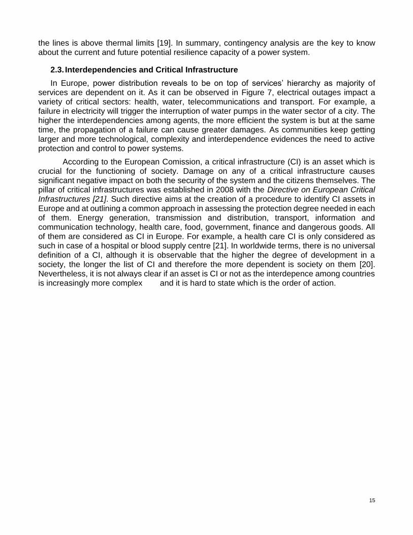
In Europe, power distribution reveals to be on top of services’ hierarchy as majority of services are dependent on it. As it can be observed in Figure 7, electrical outages impact a variety of critical sectors: health, water, telecommunications and transport. For example, a failure in electricity will trigger the interruption of water pumps in the water sector of a city. The higher the interdependencies among agents, the more efficient the system is but at the same time, the propagation of a failure can cause greater damages. As communities keep getting larger and more technological, complexity and interdependence evidences the need to active protection and control to power systems.

According to the European Comission, a critical infrastructure (CI) is an asset which is crucial for the functioning of society. Damage on any of a critical infrastructure causes significant negative impact on both the security of the system and the citizens themselves. The pillar of critical infrastructures was established in 2008 with the Directive on European Critical Infrastructures [21]. Such directive aims at the creation of a procedure to identify CI assets in Europe and at outlining a common approach in assessing the protection degree needed in each of them. Energy generation, transmission and distribution, transport, information and communication technology, health care, food, government, finance and dangerous goods. All of them are considered as CI in Europe. For example, a health care CI is only considered as such in case of a hospital or blood supply centre [21]. In worldwide terms, there is no universal definition of a CI, although it is observable that the higher the degree of development in a society, the longer the list of CI and therefore the more dependent is society on them [20]. Nevertheless, it is not always clear if an asset is CI or not as the interdepence among countries is increasingly more complex and it is hard to state which is the order of action.

16

Figure 7 - Impacts of an electricity failure on other supply services [22]

2.4. Assessment of impacts in critical events

The need to strengthen the continuity of supply has resulted in the description of a set various resilience management assessment tools in European projects, such as RESILENS. The objective of such project is to develop a “European Resilience Management Guideline” able to support all critical infrastructures in case of outages and to tackle cascading effects. The proposed assessment is both quantitative and qualitative, which are both reflected on the operational procedure proposed. The assessment encompasses three stages: 1. pre-fault (prepare, prevent and protect), 2. during fault (mitigate, absorb and adapt) and 3. post-fault (respond, recover and learn). For each stage, there are three levels: physical, operational and organizational. And for every intersection of the matrix, a set of indices are calculated [23]. Until now, all resilience projects carried out under European funding, including RESILENS, have been outlining generic strategies to increase resilience, leaving the specific solutions for each service open to debate. The novelty of the RESCCUE project, which is being developed at the moment, is a multi-sectorial approach with specific problems and solutions. For instance, in the electrical sector of Barcelona, static analysis will be carried out to study the outcome of the system in relation to CIs and other city services, such as water management.

17

It is crucial to differentiate between the concept resilience and reliability. The latter refers to the power quality delivered by the system and for which the Institute of Electrical and Electronics Engineers (IEEE), in the Standard 1366, proposed to quantify based on the continuity of supply, resulting in three main system-oriented categories: generation/transmission, customer and load. Most of the indices specified by IEEE need information about the reliability of the system, i.e. duration and frequency of the interruptions. As per data limitations of the present study, only the index of Non-Delivered Power (NDP) is calculated, which is included within the generation/transmission system-oriented indices and it is defined as the power not supplied by the system during a failure i.e. the load unsupplied.

Even though reliability and resilience are interlinked, they are not mutually inclusive. While reliability is seen as the objective of the power system, resilience deals with the preparedness and response to extreme events. As per the present times, stating resilience metrics of a power system is an on-going complex task as it must take into consideration the influence of man-made operational decisions, interconnectedness between generation and consumers or the degree of DG units in the system. Therefore, for the project under study, a mix between planning conditions (described in chapter 2.1) and the NDP index are considered to analyse the resilience of the power system.

2.5. Applicable resilience measures

The Intergovernmental Panel on Climate Change (IPCC) states in its report on Climate Change in 2014 that adaptation and mitigation measures are complementary in addressing climate change response. Both measures must be under certain enabling factors such as effective institutions, access to information and environmentally-friendly infrastructures. Adaptation refers to the procedure of adjustment to current or expected future climate effects in order to soften or avoid such harm while mitigation measures deal with the reduction of emissions of fossil fuel-based sources [24]. Adaptation and mitigation are both considered essential to increase the resilience of a power system but certainly, there are trade-offs and synergies among each other, as observed in Figure 8, in which exemplary actions are described.

Figure 8 - Adaptation and Mitigation measures in climate change [24]

18

As specific electrical actions to improve the resilience of distribution power systems, a list of adaptation and mitigation measures are described below:

- Meshed operation: supply continuity is strengthened as loads rely on more than one feeder. For example, in case of a failure, a meshed network results in reduced voltage drops and power losses, compared to a radial network [20]. Especially in cities, where underground lines are highly present, the meshed configuration in the network is more logic than ever as underground repair is very slow compared to overground reparation [20].

- Integration of DG units: the decentralization of the power system by placing DG units enhances the continuity of supply. Spatial diversification of renewable generators and energy storage, including vehicle-to-grid (V2G), enable to lessen the stress of network components and to decrease the vulnerability in critical events. Moreover, redundancy is crucial in resilience e.g. increasing number of renewable generating units and storage as back-up of conventional systems [25]. DG units reduce system losses as distance between generation and consumption is shortened and DG also decreases peak power demand, which is the base for designing new installations. The more renewable DG, the less dependence on foreign primary resources.

- Islanded microgrids: during a blackout, DG units can disconnect from the main grid to keep on supplying loads (especially critical loads), which gives flexibility to the system for repairing damaged components. In the earthquake and tsunami that struck Japan in 2011, and the consequent damage to the Fukushima nuclear power plant, the batteries of electric vehicles served as back-up generation. Such novelty resulted in the rocketing of V2G capabilities [26]. Regulatory frameworks, dynamic controls, interconnection switches and storage are essential in forming a microgrid for load restoration [27].

- Automation and communication: in a decentralised distribution grid, remotely-controlled switches will allow self-healing or automatic reconfiguration after a failure. In self-healing, there is an emergency stage where the system is quickly placed under safer conditions and secondly, a restoration stage where re-shaping of the grid happens but changing settings automatically [27]. Communication and especially local communication becomes essential if the network is performing as a microgrid.

3. Methodology

In the present study, a testing distribution system is modelled and used for simulations in order to analyse the resilience of MV and LV networks during a contingency. The static studies carried out serve as a base for further static and dynamic analysis that will be carried out within the RESCCUE Project.

The testing system model is based on the European version of the CIGRE benchmark system of 2013, as described in chapter 3.1. The model is implemented and simulated with the software DIgSILENT PowerFactory 2017, as described in chapter 3.2.

3.1. CIGRE benchmark model

To have a clear idea on the order of magnitude of the CIGRE benchmark model at MV and LV and how it can be replicated, it is helpful to know the electrical consumption of a city. For instance, in the case of Barcelona, the total electrical consumption in 2015 was of 6,781 GWh, out of which 2,156 GWh belonged to residential consumption [28].

19

For confidential reasons, the specific characteristics of the single components in the CIGRE benchmark will not be described although a general overview will be given.

3.1.1. Medium voltage network

The system at MV is three-phase and it can have either radial or meshed topology, depending on the combination of the switches, as observed in Figure 9.

Figure 9 - European CIGRE MV distribution system [29]

A description of the three phase MV system at a frequency of 50 Hz is given (refer to Figure 9):

- HV Bus and external grid: there is one bus at 110kV connected to an external grid, which represents the HV grid equivalent.

- Primary Substations: there are two substations of HV/MV with 110/20kV transformers, both with 25 MVA of rated power. The transformers have an on-load automatic control on the MV side regarding the tap position, which allows the voltage to range between 0.9 p.u. and 1.1 p.u. The HV side has a no-load tap position control with a voltage ranging from 0.95 p.u. to 1.05 p.u.

- Feeders: there are two MV feeders, each one fed from one primary substation.

20

- MV Buses: there are 14 ungrounded buses at 20kV.

- MV Loads: there are 46,215 kVA balanced peak loads (three-phase and in wye connection) which are represented as lumped with MV/LV transformers (with no control actions). It is important to state that the loads at Bus 1 and Bus 12 represent 87% of the total load of the modelled network since they represent additional feeders that are not part of Feeder 1 nor Feeder 2. In the following Table 2, the list of MV loads can be observed:

Table 2- European CIGRE MV Load parameters [own source]

Bus

Apparent Power, S [kVA] Power Factor, pf

Residential Commercial/ Industrial

Residential Commercial/ Industrial

1 15300 5100 0.98 0.95

2 - - - -

3 285 265 0.97 0.85

4 445 - 0.97 -

5 750 - 0.97 -

6 565 - 0.97 -

7 - 90 - 0.85

8 605 - 0.97 -

9 - 675 - 0.85

10 490 80 0.97 0.85

11 340 - 0.97 -

12 15300 5280 0.98 0.95

13 - 40 - 0.85

14 215 390 0.97 0.85

- Switches: there are three switches (S1, S2 and S3) and two modes (open or close) which result in eight possible configurations (observe Figure 9 for further clarification).

- Lines: the lines in Feeder 1 are underground while the lines in Feeder 2 are over ground. Both lines are untransposed (mutual coupling between phases) and therefore unbalance in the system is present.

3.1.2. Low voltage network

The system at LV is three-phase and it has a radial topology, as observed in Figure 10.

21

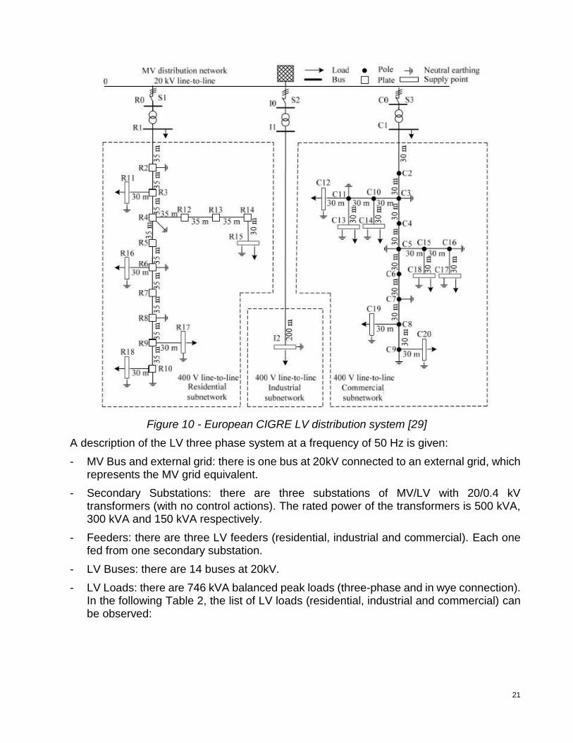
Figure 10 - European CIGRE LV distribution system [29]

A description of the LV three phase system at a frequency of 50 Hz is given:

- MV Bus and external grid: there is one bus at 20kV connected to an external grid, which represents the MV grid equivalent.

- Secondary Substations: there are three substations of MV/LV with 20/0.4 kV transformers (with no control actions). The rated power of the transformers is 500 kVA, 300 kVA and 150 kVA respectively.

- Feeders: there are three LV feeders (residential, industrial and commercial). Each one fed from one secondary substation.

- LV Buses: there are 14 buses at 20kV.

- LV Loads: there are 746 kVA balanced peak loads (three-phase and in wye connection). In the following Table 2, the list of LV loads (residential, industrial and commercial) can be observed:

22

Table 3 - European CIGRE LV Load parameters [own source]

Bus Apparent Power, S [kVA] Power Factor, pf

R1 200 0.95

R11 15 0.95

R15 52 0.95

R16 55 0.95

R17 35 0.95

R18 47 0.95

I2 100 0.85

C1 120 0.90

C12 20 0.90

C13 20 0.90

C14 25 0.90

C17 25 0.90

C18 8 0.90

C19 16 0.90

C20 8 0.90

- Lines: lines in the residential and industrial feeders are underground while lines in the commercial feeder are overhead. Both lines are untransposed (mutual coupling between phases) and therefore unbalance in the system is present.

3.2. DIgSILENT PowerFactory

The modelling and simulations are implemented in DIgSILENT 2017, a power system analysis software. The models of MV and LV seen in Figure 9 and Figure 10, respectively, are combined together for the purpose of the study. The MV system is modelled with lumped loads, except for Bus 2, in which the insertion of the LV grid into the MV grid takes place, even though at a DSO level, studies are generally carried out only with the MV model. The only reason why the LV grid is modelled at Bus 2 is to be aware of the response at the last distribution network part before arriving to the end consumers.

As observed in Figure 11a), the grid at 100kV consists of the HV equivalent grid and Bus 0, both present in previous Figure 9. In Figure 11b), Substation 1 is observed and it stands for both the HV/MV transformer and Bus 1, present in previous Figure 9 (parallel structure is modelled for Substation 2, which includes Bus 12).

23

(a)

(b)

Figure 11 – (a) HV Grid and (b) Substation 1 with DIgSILENT [own source]

Regarding the buses within Feeder 1 and Feeder 2 observed in Figure 9, each one of the buses belongs to a Distribution Centre within DIgSILENT in order to resemble reality, as obseved in Figure 12, where the two big circles represent Substations and the twelve small circles represent Distribution Centres. Feeder 1 encompasses the following Distribution Centres: 2, 3, 4, 5, 6, 7, 8, 9, 10 and 11. For Feeder 2, both Distribution Centre 13 and 14 are included.

Figure 12 - Overview of the MV distribution network with DIgSILENT in radial topology [own source]

24

In Figure 13a), the unique Distribution Centre 2 with the LV integrated (randomly chosen) is observed. In Figure 13b), the Distribution Centre 3 with MV aggregated loads is representative of how the remaining ten Distribution Centres are modelled.

(a)

(b)

Figure 13 – (a) Distribution Centre 2 and (b) Distribution Centre 3 with lumped loads with DIgSILENT [own source]

Finally, in Figure 14, the LV distribution network is modelled. As observable, in the LV grid there are other feeders appearing since voltage has been stepped down. There are the residential, the industrial and the commercial feeders, which always operate radially.

(a)

(b)

Figure 14 - (a) LV Grid and b) close-up view of the LV Grid with DIgSILENT [own source]

Before running the simulations for the present study, an initial validation of the network modelled with DIgSILENT is carried out based on the power flow results given by the CIGRE benchmark model of 2013, with no simulation software specified. Concerning the voltage in the buses of the MV grid (Figure 9), DIgSILENT results have a maximum error of 1.67% compared to CIGRE results and regarding the voltage in the buses of the LV grid (Figure 10), DIgSILENT results have a maximum error of 1.80% compared to CIGRE results. From such errors, it can be stated that the model properly fits with the one used and proposed by CIGRE.

25

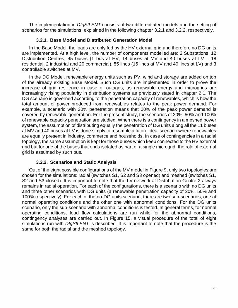
The implementation in DIgSILENT consists of two differentiated models and the setting of scenarios for the simulations, explained in the following chapter 3.2.1 and 3.2.2, respectively.

3.2.1. Base Model and Distributed Generation Model

In the Base Model, the loads are only fed by the HV external grid and therefore no DG units are implemented. At a high level, the number of components modelled are: 2 Substations, 12 Distribution Centres, 45 buses (1 bus at HV, 14 buses at MV and 40 buses at LV – 18 residential, 2 industrial and 20 commercial), 55 lines (15 lines at MV and 40 lines at LV) and 3 controllable switches at MV.

In the DG Model, renewable energy units such as PV, wind and storage are added on top of the already existing Base Model. Such DG units are implemented in order to prove the increase of grid resilience in case of outages, as renewable energy and microgrids are increasingly rising popularity in distribution systems as previously stated in chapter 2.1. The DG scenario is governed according to the penetration capacity of renewables, which is how the total amount of power produced from renewables relates to the peak power demand. For example, a scenario with 20% penetration means that 20% of the peak power demand is covered by renewable generation. For the present study, the scenarios of 20%, 50% and 100% of renewable capacity penetration are studied. When there is a contingency in a meshed power system, the assumption of distributing equally the penetration of DG units along all the 11 buses at MV and 40 buses at LV is done simply to resemble a future ideal scenario where renewables are equally present in industry, commerce and households. In case of contingencies in a radial topology, the same assumption is kept for those buses which keep connected to the HV external grid but for one of the buses that ends isolated as part of a single microgrid, the role of external grid is assumed by such bus.

3.2.2. Scenarios and Static Analysis

Out of the eight possible configurations of the MV model in Figure 9, only two topologies are chosen for the simulations: radial (switches S1, S2 and S3 opened) and meshed (switches S1, S2 and S3 closed). It is important to note that the LV network at Distribution Centre 2 always remains in radial operation. For each of the configurations, there is a scenario with no DG units and three other scenarios with DG units (a renewable penetration capacity of 20%, 50% and 100% respectively). For each of the no-DG units scenario, there are two sub-scenarios, one at normal operating conditions and the other one with abnormal conditions. For the DG units scenario, only the sub-scenario with abnormal conditions is tested. In general terms, for normal operating conditions, load flow calculations are run while for the abnormal conditions, contingency analyses are carried out. In Figure 15, a visual procedure of the total of eight simulations run with DIgSILENT is described. It is important to note that the procedure is the same for both the radial and the meshed topology.

26

Figure 15 - Procedure of the simulations run for each network topology [own source]

In order to analyse the behaviour of the grid in static mode and to find out how resilient it is, both load flow and contingency analysis are carried out. The power flow undergoing during both load flow and contingency analysis is balanced according to the reference/slack machine, which must ensure the power balance of the network. Being a reference machine means that both the active and reactive power are a result of the power flow while voltage magnitude and phase shift are fixed. When the grid is connected to the main HV equivalent grid, such external grid plays the role of the reference machine. But when there is a static contingency and a part of the network becomes islanded, DIgSILENT’s limitations force to place a reference machine, a synchronous generator, in the new microgrid formed in order for the power flow to run properly. Out of all the Distribution Centres that remain islanded as one single microgrid during the contingency event, and after several “trial-and-error”, Bus 9 within the Distribution Centre 9 is chosen to have the reference machine connected. The latter is simply chosen for software limitation purposes since an islanded microgrid must contain a reference machine in order to run the simulation on DIgSILENT. Therefore, such software limitations regarding static analyses with islanded microgrid, leads to initially fixing the amount of load to be supplied e.g. 20% of the load is supplied when there is a renewable penetration capacity of 20%.

The contingency analyses carried out during all Sub-scenario 2 cases consist of the outage of the line connecting Distribution Centre 3 to Distribution Centre 8. The choice of such line has been chosen randomly, since it is supposed to resemble a real-life situation in which the failed component is not necessarily the element with the highest load. For instance, in heavy rainfalls, the most probable component to trip in a city might simply be one of the numerous underground lines.

27

4. Results and Discussion

The process described in chapter 3.2 leads to an analysis where the results obtained from the ten simulations, five for radial topology and five for meshed topology, outlined in Figure 15 are evaluated. Regarding the nomenclature used for the Busbars in the present analysis, both buses at MV and LV keep the names observed in Figure 9 and Figure 10, respectively. When referring in terms of Substations and Distribution Centres, the nomenclature is that of Figure 12. Due to the large number of results, these are discussed immediately after the presentation of such.

4.1. Normal Operation with the Base Model

The present simulation resembles the situation of normal operating conditions in a network with no DG units and being the HV external grid the only component supplying power to the loads.

4.1.1. Radial Configuration

In a radial topology, where loads are only connected to one Distribution Centre, the voltage level at each bus is shown in Figure 16 and Figure 17.

Figure 16 - Voltage level at the MV buses in normal conditions and radial operation [own source]

28

Figure 17 – Voltage level at the LV buses in normal conditions and radial operation [own source]

It can be seen in Figure 16 that the voltage at Bus 1 is at 1.025 p.u., which is 2.5% above the rated voltage of 20kV. Throughout the MV grid the voltage does not drop below 0.979 p.u. (Bus 11). Therefore, voltage level remains within the acceptable DSO range of 0.9 and 1.1 p.u. Regarding Figure 17, the voltage level at the 0.4 kV grid is between 0.889 p.u. in Bus C13 and 0.969 p.u. in Bus R1. At present times, DSOs do not analyse the LV grids and therefore the results cannot be compared to a real-life voltage range.

In the following Figure 18, the voltage profile within Substation 1 and Feeder 1 can be observed, where the x-axis represents the distance in km and the y-axis represents the voltage level in p.u.

29

Figure 18 - Voltage profile at buses in Feeder 1 in normal conditions and radial operation [own source]

In the above graph, it is patent how the distance influences voltage level. Since the lines in the network are untransposed and hence they add unbalance to the system, it is clear that the further away from Substation 1, the more the voltage drops. But voltage drop is not only dependant on the length of the path, but also to the amount of loads interrupting the path. For instance, Bus 11 presents the lowest voltage in the MV grid but Bus 7 is the one at highest distance from the supply. Since there are fewer loads to feed before reaching Bus 7, the voltage drop is not as accentuated. Therefore, the amount of loads affects more the voltage drop than the unbalances of lines. With respect to the buses in the LV grid Figure 18, shows a visual picture where all the LV buses suffer a considerable voltage drop in comparison to the MV buses, as expected. Moreover, during the simulation, each line with a loading superior to 80% of its capacity is considered overloaded and hence appeared as red coloured. In this case, overloading only occurs in the line connecting Bus C3 to Bus C10. In the following Table 4, a list of the five most loaded lines in the LV and MV grid is shown.

30

Table 4 – Line parameters in normal conditions and radial operation [own source]

Line Loading [%] Losses [kW] Active Power [MW] Reactive Power [Mvar]

C3-C10 97.31 1.29 0.06 0.03

C10-C11 60.12 0.49 0.04 0.02

C1-C2 56.25 1.68 0.12 0.06

C2-C3 56.25 1.68 0.12 0.06

R6-R16 54.25 0.53 -0.05 -0.02

1-2 48.40 50.95 5.15 1.84

2-3 41.47 58.77 4.39 1.40

3-8 20.58 4.26 2.12 0.73

3-4 16.08 1.22 1.71 0.38

9-8 14.36 0.51 -1.45 -0.58

It is observable how lines in the MV grid are less loaded, which is due to the fact that the cables are designed at a higher nominal current. In a hypothetical case where load is added further down Bus C10, the line C3-C10 should be replaced by one with greater capacity as it is already overstressed. Meanwhile, losses, active and reactive power are of bigger magnitude in the MV grid as the power flowing through the lines is considerably greater.

There are zero unsupplied loads, NDP is zero, since all the power is being supplied by the external grid, which works as a reference machine and is in charge of supplying a total of 48.69 MVA. The total load of the network is 46.96 MVA, which is lower than the generation of the external grid because the network suffers losses and the external grid needs to, obviously, supply power to meet the load requirements. By applying Equation 1, the losses in the network are calculated.

𝑁𝑒𝑡𝑤𝑜𝑟𝑘 𝑙𝑜𝑠𝑠𝑒𝑠 (%) = (0.238 + 0.36 + 0.002 + 0.02) 𝑀𝑊

45.75 𝑀𝑊𝑥 100 = 1.36 %

It is remarkable to state that transformer losses are mainly due to core losses and therefore they just depend on the transformer manufacturing settings. Observing at the network losses, both MV and LV lines suffer greater losses than transformers. Comparing lines, power flow has a bigger influence on the losses since in the MV lines the power flowing is greater as there is more load downstream and therefore, more current is flowing, which leads to greater ohmic losses.

In Table 5, the loading of the transformers is analyzed, as the grid expansion capacity is highly dependent on the transformers.

Table 5 - Transformer parameters in normal conditions and radial operation [own source]

Transformer Loading [%]

31

MV/LV Residential 86.92

MV/LV Industrial 72.33

MV/LV Commercial 87.63

HV/MV Substation 2 87.51


It can be observed how all transformers are working close to their nominal capacity, which is common in real life networks. In Substation 1, the transformer is working above its nominal capacity since the technical parameters introduced in PowerFactory might be too limiting, although such parameters have been chosen as the adequate after the model validation mentioned in chapter 3.2. Anyways, since the future in electrical is moving towards renewable DG, a transformer working close to nominal capacities is not a critical issue as their loading will be decreased.

4.1.2. Meshed Configuration

When meshing the MV grid, loads are no longer fed from just one single point and therefore the resilience of the grid increases. In Figure 19 and Figure 20 the voltage level within the network is shown.

Figure 19 - Voltage level at the MV buses in normal conditions and meshed operation [own source]

32

Figure 20 - Voltage level at the LV buses in normal conditions and meshed operation [own source]

Observing Figure 19, voltage at the MV meshed grid ranges from 0.981 p.u. to 1.024 p.u., which compared to the voltage at the MV radial grid shown in Figure 16 leads to the expected results. In a meshed grid, the voltage deviations from the rated value are less frequent as the power flow has more path possibilities. Regarding Figure 20, the voltage level at the LV grid is between 0.886 p.u. and 0.968 p.u. The latter cannot be stated as acceptable or not since DSOs only work at MV levels when performing static studies.

The amount of power that the lines in the system are able to withstand sheds light to the expansion capacity of the grid. Again, the superior limit of 80% loaded is considered and all lines above this value are considered overloaded and hence expansion constraints. In Table 6, a list of the five most lines in the LV and MV grid is shown.

Table 6 - Line parameters in normal conditions and meshed operation [own source]


C3-C10 97.63 1.29 0.06 0.03

C10-C11 60.32 0.49 0.04 0.02

C2-C3 56.43 1.69 0.12 0.06

C1-C2 56.43 1.69 0.12 0.06

R6-R16 54.33 0.53 -0.05 -0.02

1-2 35.88 27.85 3.22 2.42

2-3 29.34 29.06 2.48 2.05

3-4 17.16 1.39 1.60 0.95

12-13 15.32 36.35 2.51 -0.43

13-14 15.15 21.75 2.44 -0.48

33

Again, as in the radial topology, lines in the MV grid are less loaded because the designing of the lines in terms of nominal current has considered bigger tolerances. Compared to the loadings during radial operation seen in Table 4, lines 3-8 and 9-8 are no longer in the top 5 and they present a decrease in loading of 29.55% and 24.23%, respectively. The reason is that the load in Bus 8 is now being fed from both Bus 3 and Bus 14, and hence distributing the power flow between two lines now. At the same time, Bus 9 is now also receiving power from both Bus 8 and Bus 10. In support to the last statements, lines 12-13 and 13-14 observed in Table 6 are significantly more loaded as they are now supplying more loads with the closure of switch S1.

All loads are supplied during a meshed operation with no outages. The 48.72 MVA of apparent power generated is fully coming from the HV equivalent external grid, while the total load is 46.96 MVA. As stated in chapter 4.1.1, the difference of 1.76 MVA is generated to counteract the unbalances of the network. By applying Equation 1, the losses in the network are calculated.


45.82 𝑀𝑊𝑥 100 = 1.42 %

During normal operating conditions, losses appear to be greater in a meshed topology than in a radial topology (chapter 4.1.1). As described in chapter 3.1, the unbalance in the network is provoked mainly by lines and therefore, in meshed operation there are connected three new lines, which imply higher losses simply because the global distance to be run by the power is bigger and therefore the losses increase.

In Table 7 the loading of the transformers is analyzed as the grid expansion capacity is highly dependent on the transformers.

Table 7 - Transformer parameters in normal conditions and meshed operation [own source]







With respect to Table 5 during radial operation, it is observable how the MV/LV transformers do not present significant changes in loading, unlike the HV/MV transformer in Substation 1. The latter decreases loading by 6.86% as Substation 1 is now connected to Substation 2 and therefore releasing congestion as the majority of the load was connected to Substation 1 in radial mode. On the contrary, the HV/MV transformer in Substation 2 is now increasing its loading by 6.97%.

4.2. Contingency with the Base Model

The outage of the line connecting Bus 3 to Bus 8 is carried out to analyse the response and resilience of the network with no DG units and therefore with the HV equivalent grid as the only source of supply.

34


In a radial topology under a contingency, the effects can be visually supported with

Figure 21, where the unsupplied Distribution Centres are coloured in grey.

Figure 21 - Overview of the distribution in a radial topology with a contingency [own source]

With the outage of line 3-8, a cascading effect takes place as all the distribution centres dependent on Distribution Centre 3, i.e. Distribution Centre 7, 8, 9, 10 and 11 become de-energized. Simultaneously, there is the tripping of all the lines interconnecting such points. In the following Figure 22 and Figure 23, the voltage profile at the MV and LV grid are shown.

35

Figure 22 - Voltage level at the MV buses in a radial topology with a contingency [own source]

Figure 23 - Voltage level at the LV buses in a radial topology with a contingency [own source]

Regarding the MV buses, and neglecting those de-energized, the voltage ranges from 0.996 p.u. to 1.031 p.u. As expected, the voltage at the buses is close to the nominal value as Feeder 1 is significantly diminished in terms of load and line lengths with the de-energization of five distribution centres. The buses at the LV grid with the lowest and highest voltage level, C13 and R1 respectively, are once again the same ones as in the scenarios of chapter 4.1.

Regarding the lines parameters after the contingency analysis, in Table 8 the five most loaded lines of both the MV and LV grid is shown.

36

Table 8- Line parameters in a radial topology with a contingency [own source]


C3-C10 82.85 0.95 0.05 0.03

C10-C11 50.88 0.36 0.03 0.02

R6-R16 48.33 0.44 -0.05 -0.02

C2-C3 48.03 1.25 0.10 0.05

C1-C2 48.03 1.25 0.10 0.05

1-2 26.71 15.55 2.91 0.85

2-3 20.42 14.19 2.23 0.54

3-4 15.65 1.16 1.71 0.38

4-5 11.70 0.59 1.28 0.28

5-6 5.06 0.30 0.55 0.11

With the outage of line 3-8, now there are only left a total of five lines being fed by Substation 1. Comparing the results in Table 8 with the results in Table 6, the loadings have decreased considerably in the lines connecting the buses upstream of Bus 3. Once again, the line C3-C10 is already working at 82.85% of its capacity and therefore, in case of adding loads downstream, the cable type should be changed to one with greater nominal current. As expected, losses and both active and reactive power are of bigger magnitude in the MV grid than in the LV grid.

Due to this contingency, all loads connected to the de-energized buses are unsupplied. Therefore, the NDP equals 2.28 MVA and the total amount of load supplied is dropped to 44.68 MVA, Meanwhile, the power supplied by the external grid has now a value of 46.13 MVA. The difference between the consumed and generated power is now shorter than in the scenario of chapter 4.1.1 simply because the amount of losses of the network, which have the cause in the untransposed lines and transformers, have shortened as the network power demand has also shortened with this outage. By applying Equation 1, the losses in the network are calculated.


43.55 𝑀𝑊𝑥 100 = 1.12 %

Observing at the network losses, again, both MV and LV lines suffer bigger losses than transformers. As there is now a contingency and load is left unsupplied, the power flowing through lines is decreased and therefore losses in this case are lower than in the radial topology under normal operation (chapter 4.1.1).

In Table 9, the loading of the transformers in the network can be observed in order to plan a possible future expansion of the system.

37

Table 9 – Transformer parameters in a radial topology with a contingency [own source]







In parallel to what has already been stated previously during this chapter, all the transformers within the affected Substation 1 and Feeder 1 present a decrease in loading as the amount of supplied load has decreased as well.


In an outage event, the meshed operation of the grid increase resilience as loads which would have been unsupplied in a radial mode can now be supplied. In Figure 24 and Figure 25, the voltage level within the network is shown.

Figure 24 - Voltage level at the MV buses in a meshed topology with a contingency [own source]

38

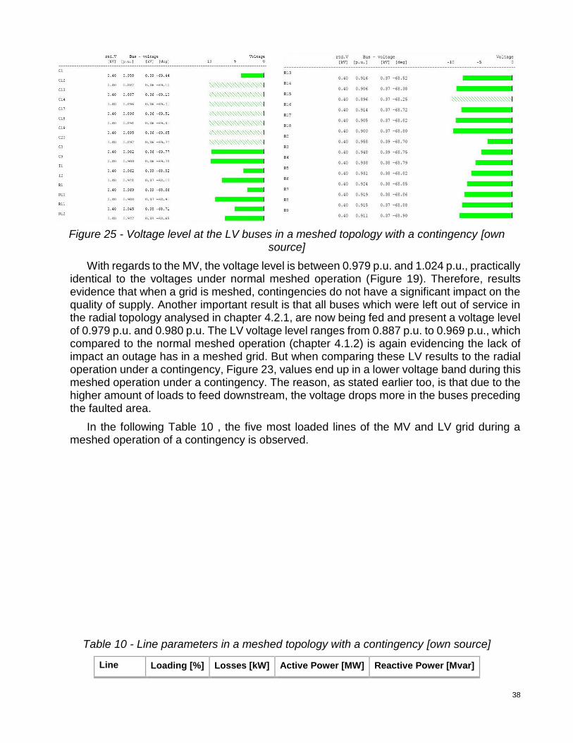
Figure 25 - Voltage level at the LV buses in a meshed topology with a contingency [own source]

With regards to the MV, the voltage level is between 0.979 p.u. and 1.024 p.u., practically identical to the voltages under normal meshed operation (Figure 19). Therefore, results evidence that when a grid is meshed, contingencies do not have a significant impact on the quality of supply. Another important result is that all buses which were left out of service in the radial topology analysed in chapter 4.2.1, are now being fed and present a voltage level of 0.979 p.u. and 0.980 p.u. The LV voltage level ranges from 0.887 p.u. to 0.969 p.u., which compared to the normal meshed operation (chapter 4.1.2) is again evidencing the lack of impact an outage has in a meshed grid. But when comparing these LV results to the radial operation under a contingency, Figure 23, values end up in a lower voltage band during this meshed operation under a contingency. The reason, as stated earlier too, is that due to the higher amount of loads to feed downstream, the voltage drops more in the buses preceding the faulted area.

In the following Table 10 , the five most loaded lines of the MV and LV grid during a meshed operation of a contingency is observed.

Table 10 - Line parameters in a meshed topology with a contingency [own source]


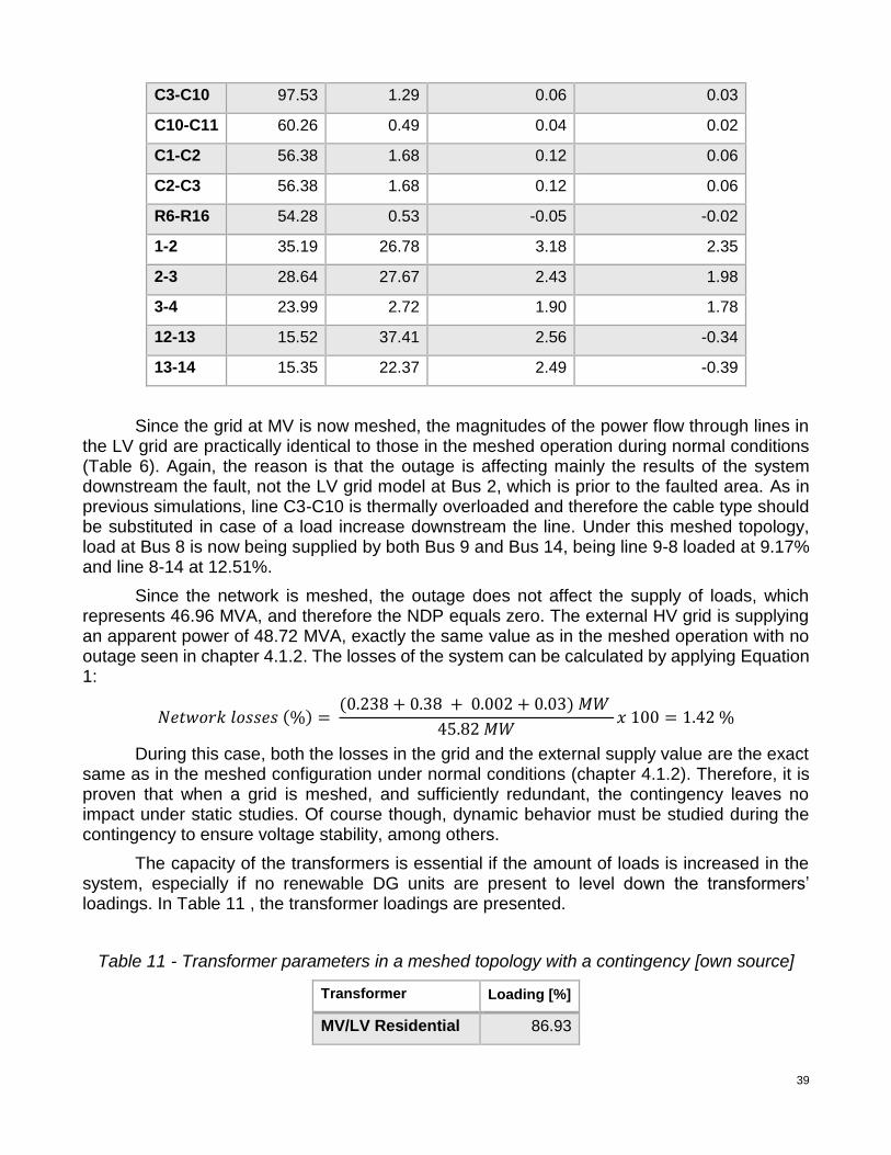
39

C3-C10 97.53 1.29 0.06 0.03

C10-C11 60.26 0.49 0.04 0.02

C1-C2 56.38 1.68 0.12 0.06

C2-C3 56.38 1.68 0.12 0.06

R6-R16 54.28 0.53 -0.05 -0.02

1-2 35.19 26.78 3.18 2.35

2-3 28.64 27.67 2.43 1.98

3-4 23.99 2.72 1.90 1.78

12-13 15.52 37.41 2.56 -0.34

13-14 15.35 22.37 2.49 -0.39

Since the grid at MV is now meshed, the magnitudes of the power flow through lines in the LV grid are practically identical to those in the meshed operation during normal conditions (Table 6). Again, the reason is that the outage is affecting mainly the results of the system downstream the fault, not the LV grid model at Bus 2, which is prior to the faulted area. As in previous simulations, line C3-C10 is thermally overloaded and therefore the cable type should be substituted in case of a load increase downstream the line. Under this meshed topology, load at Bus 8 is now being supplied by both Bus 9 and Bus 14, being line 9-8 loaded at 9.17% and line 8-14 at 12.51%.

Since the network is meshed, the outage does not affect the supply of loads, which represents 46.96 MVA, and therefore the NDP equals zero. The external HV grid is supplying an apparent power of 48.72 MVA, exactly the same value as in the meshed operation with no outage seen in chapter 4.1.2. The losses of the system can be calculated by applying Equation 1:


45.82 𝑀𝑊𝑥 100 = 1.42 %

During this case, both the losses in the grid and the external supply value are the exact same as in the meshed configuration under normal conditions (chapter 4.1.2). Therefore, it is proven that when a grid is meshed, and sufficiently redundant, the contingency leaves no impact under static studies. Of course though, dynamic behavior must be studied during the contingency to ensure voltage stability, among others.

The capacity of the transformers is essential if the amount of loads is increased in the system, especially if no renewable DG units are present to level down the transformers’ loadings. In Table 11 , the transformer loadings are presented.

Table 11 - Transformer parameters in a meshed topology with a contingency [own source]



40





All the transformers are working close to its nominal capacity, being the transformer at Substation 1 above its capacity. Once again, differences between the results of a meshed topology under normal operations or a contingency are so insignificant that it can be stated that when a grid is meshed, resilience is assured.

4.3. Contingency with Distributed Generation

Under a contingency event such as the outage of the line connecting the Distribution Centre 3 to the Distribution Centre 8, the DG units along the grid will supply the necessary power, together with the HV external grid, to keep the system balanced under steady state. The results obtained with the different amounts of renewable DG penetration capacity aim to prove the increase of resilience after a fault.


After a fault, if a radial topology with DG is implemented in the network, the results depend highly on the percentage of renewable penetration capacity, especially in the faulted area. In the following chapters, percentages of 20%, 50% and 100% of renewable penetration capacity are analysed. During the studies, each load to be supplied is demanding its peak load, although the necessary load shedding is implemented in order to keep the system balanced.

4.3.1.1. Renewable penetration capacity of 20%

The amount of load supplied from renewable DG units is 20%, while the remaining 80% of the load is supplied by the external grid. In the following Figure 26 and Figure 27, the voltage levels can be observed.

41

Figure 26 - Voltage level at the MV buses under a contingency in a radial topology with 20% of renewable penetration capacity [own source]

Figure 27 - Voltage level at the LV buses under a contingency in a radial topology with 20% of renewable penetration capacity [own source]

By adding DG units, the MV grid has improved voltage levels in all buses, being now the voltage range between 0.998 p.u. and 1.032. Therefore, by only applying a distributed renewable penetration of 20% in an outage event, the voltage level has already improved compared to the energized buses of chapter 4.2.1. For example, the Distribution Centres 7,8,9,10 and 11, which were out of service during the outage under a radial topology with no DG units, are now at nominal voltage. Regarding the LV grid, whose voltage level goes from 0.932 p.u. to 0.995 p.u., it makes sense to compare results to the radial configuration under normal conditions (chapter 4.1.1) to analyse the difference between feeding the buses with DG units or with the external grid. With the implementation of the DG units, it can be observed how the lower voltage limit increases by 4.3% while the upper voltage limit increases by 2.6%.

With regards to the line loadings, in Table 12 , the most loaded line in the LV and MV grid can be observed.

42

Table 12 – Line parameters under a contingency in a radial topology with 20% of renewable penetration capacity [own source]


C3-C10 74.47 0.75 0.05 0.02

1-2 21.49 10.02 2.35 0.64

In this present radial configuration, all line loadings have been found to be the lowest analysed so far, which is the expected behaviour since distributed renewable sources give flexibility to the system and release electrical stress in lines and transformers. The loading of the lines observed is simply due to the 80% of remaining load supply that is coming from the external grid. Therefore, the more renewable DG units implemented, the less electrical stress all the grid components will suffer, a fact that is also proven by looking at the transformer loadings in Table 13. Evidently, there are added challenges, as explained in chapter 2.1, as adapting technology and dealing with the variability of renewable sources.

Table 13 - Transformer parameters under a contingency in a radial topology with 20% of renewable penetration capacity [own source]







In the unfaulted area, all loads are fed, while the on-outage area that has become a single microgrid suffers losses in the load supply. In total, the loads supplied add up to 45.14 MVA, which translates to 1.82 MVA of NDP or 4% of the supply lost. Regarding the total losses in the network, in Equation 1 the value is calculated.


(34.84 + 9.08) 𝑀𝑊𝑥 100 = 0.78 %

Network losses, as expected, decrease significantly compared to all previous results since with the implementation of DG, generation is now closer to consumption, and therefore line power flows are reduced since local renewable sources are attached directly to the same node as the load. Converter losses have not been considered in the analysis.


By applying a renewable penetration capacity of 50% in the grid and the remaining 50% coming from the external grid, the MV results with respect to voltage level are seen in Figure 28 and Figure 29.

43

Figure 28- Voltage level at the MV buses under a contingency in a radial topology with 50% of renewable penetration capacity

Figure 29 - Voltage level at the LV buses under a contingency in a radial topology with 50% of renewable penetration capacity

The MV voltage is ranging now from 1 p.u. to 1.036 p.u and for the first time in the present study, the voltage level is never below the nominal in the MV grid. The fact that the voltage is increased proves the challenges of integrating DG, as the voltage profile in a network is threatened of increasing above the acceptable limits of a DSO. The fact that static studies evidence increase in voltage due to the converters of the DG, dynamic simulations gain importance in order to maintain voltage stability with the penetration of distributed renewable energy. Regarding the LV voltage levels, the profile is exactly the same as in Figure 27 but values vary slightly, being the voltage lower limit a 4.6% higher and the upper voltage limit a 2.1% higher.

In Table 14, the lines with the highest loading in both the LV and MV network are observed.

44

Table 14 - Line parameters under a contingency in a radial topology with 50% of renewable penetration capacity [own source]


C3-C10 44.50 0.27 0.03 0.01

1-2 13.12 3.74 1.46 0.30

With respect to the case of 20% renewable penetration in chapter 4.3.1.1, the loading now in the LV line C3-C10 has decreased by 29.97% while the MV line 1-2 has decreased by 8.37%. It can be assured that the impact DG units have on LV lines is greater than in MV lines. When analysing the DG impact on transformers, Table 15 shows the results to be analysed.








Meanwhile, DG impact presents no great differences between HV/MV and MV/LV transformers. In average, HV/MV transformers decrease by 27.86% while MV/LV transformers only by a 24.76% when comparing to the 20% renewable case. Therefore, it cannot be affirmed that transformers in the LV grid suffer more or less the DG impact than those in the MV grid.

The load supplied during this case is 45.80 MVA, which means that there are 1.16 MVA of NDP or 2% of load loss. If looking at the network losses, the value can be calculated by applying Equation 1.


(21.75 + 22.72) 𝑀𝑊𝑥 100 = 0.42%

Under a renewable penetration capacity of 50%, network losses are practically non-existent. The low amount of power flowing through lines leads to losses which are practically zero.


By having all load supplied from DG units, voltage levels have the values seen in Figure 30.

45

Figure 30 - Voltage level at the MV buses under a contingency in a radial topology with 100% of renewable penetration capacity

The voltage level at MV within this case is ranging from 1 p.u. to 1.052 p.u., which compared to the 50% renewable case presented in 4.3.1.2 represents an increase in the upper bound voltage of 1.6%. The resulted voltage range goes is line with the typical voltage range of DSOs, which is placed in ±10%. Therefore, in terms of static studies, DG units do not present a problem for the network tolerances in terms of voltage. Still, rapid increases in voltage due to sudden increase of photovoltaic panels, for example, evidences the need of having an active and real-time control over grid with a high penetration of renewable energy. Regarding the LV level, all buses in the grid are at exactly 1.051 p.u., which shows the stability the grid gains when the generation is decentralized.

With regards to line parameters, values of the most loaded lines in both the LV and MV can be observed in Table 16.

Table 16 - Line parameters under a contingency in a radial topology with 100% of renewable penetration capacity [own source]


C3-C10 0.00 0.00 0.00 0.00

1-2 1.73 0.05 0.00 -0.20

In line with the stability in the voltage level at the LV grid, the lines in the LV grid present such a small power flow that it can be rounded to zero when there are only two decimals. In the MV line 1-2 though, losses are more significant simply because the amount of power flowing is bigger. The reason why there is power flowing through lines is because transformers have inherent manufacturing losses and therefore the external grid, as a reference machine, has to balance out the power. When paying attention to the transformers, Table 17 shows the results to be analysed.

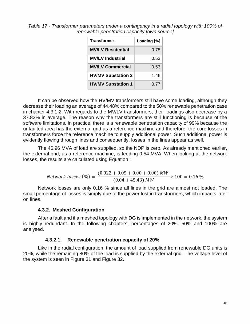
46








It can be observed how the HV/MV transformers still have some loading, although they decrease their loading an average of 44.48% compared to the 50% renewable penetration case in chapter 4.3.1.2. With regards to the MV/LV transformers, their loadings also decrease by a 37.82% in average. The reason why the transformers are still functioning is because of the software limitations. In practice, there is a renewable penetration capacity of 99% because the unfaulted area has the external grid as a reference machine and therefore, the core losses in transformers force the reference machine to supply additional power. Such additional power is evidently flowing through lines and consequently, losses in the lines appear as well.

The 46.96 MVA of load are supplied, so the NDP is zero. As already mentioned earlier, the external grid, as a reference machine, is feeding 0.54 MVA. When looking at the network losses, the results are calculated using Equation 1


(0.04 + 45.43) 𝑀𝑊𝑥 100 = 0.16 %

Network losses are only 0.16 % since all lines in the grid are almost not loaded. The small percentage of losses is simply due to the power lost in transformers, which impacts later on lines.


After a fault and if a meshed topology with DG is implemented in the network, the system is highly redundant. In the following chapters, percentages of 20%, 50% and 100% are analysed.


Like in the radial configuration, the amount of load supplied from renewable DG units is 20%, while the remaining 80% of the load is supplied by the external grid. The voltage level of the system is seen in Figure 31 and Figure 32.

47

Figure 31 - Voltage level at the MV buses under a contingency in a meshed topology with 20% of renewable penetration capacity [own source]

Figure 32 - Voltage level at the LV buses under a contingency in a meshed topology with 20% of renewable penetration capacity [own source]

In the MV system, the voltage ranges from 0.990 p.u. to 1.031 p.u., which compared to the 20% penetration in radial mode (chapter 4.3.1.1) evidences the difference between a meshed and a radial system on the faulted area. In the radial mode, all the buses on the faulted area form a single power island and their voltage level is exactly the nominal voltage. Meanwhile, in this meshed mode, there is no isolation of the faulted area and the voltage is no longer the nominal but a lower voltage. Clearly, in case of a fault, it is more stable to maintain the faulted area isolated than to mesh it with the unfaulted grid. The LV system, as it always has a radial operation, behaves as expected. Since the bus from where the LV system is connected, Bus 2, is now at 1.016 p.u. while in the radial mode with 20% penetration (chapter 4.3.1.1) it was at 1.025 p.u., all the voltage in the LV buses present lower values.

The most loaded line in both the LV and MV grid are presented in Table 18.

48

Table 18 – Line parameters under a contingency in a meshed topology with 20% of renewable penetration capacity [own source]


C3-C10 75.13 0.77 0.05 0.02

1-2 30.34 19.94 2.70 2.11

The C3-C10 line is below 80% loaded, and it is around 20% less loaded than in the case of meshed operation and no DG units under a contingency (chapter 4.2.2). As expected, this decrease in loading is due to the penetration of renewable energy, which releases line stresses. When observing line 1-2 and comparing it to the chapter 4.2.2 results too, the decrease in loading is exactly 4.85%. Since the MV grid is the only part of the network meshed, it is remarkable to state that when the penetration of renewables is 20%, the most loaded line in the MV grid decreases by around 5% its stress.

As the grid is meshed, all the 46.96 MVA of load are fully supplied by both the external grid and the DG units. This time, the HV grid is feeding 38.70 MVA while the DG units are supplying 9.39 MVA. The total losses in the network are calculated with Equation 1:


(36.61 + 9.08) 𝑀𝑊𝑥 100 = 0.95 %

Evidently, network losses are decreased compared to the case with no DG units (chapter 4.2.2) since lines suffer less stress and therefore losses are automatically decreased as well. With DG units introduced in the system, the loading of transformers is decreased as it can be observed in Table 19.

Table 19 - Transformer parameters under a contingency in a meshed topology with 20% of renewable penetration capacity [own source]







Again, if comparing to the case with no DG units seen in chapter 4.2.2, all transformers in the network are 20% less loaded. The HV/MV transformer of Substation 1 is at risk of overloading in case of a load increase in the system as it is already 80.80% loaded.


With a 50% capacity of renewable penetration, voltage value of both the MV and LV system in the network can be observed in Figure 33 and Figure 34, respectively.

49


Figure 34 - Voltage level at the LV buses under a contingency in a meshed topology with 50% of renewable penetration capacity [own source]

Due to a 50% of renewable penetration and a meshed operation, the voltage profile at MV is now between 1.009 p.u. and 1.037 p.u., being the Distribution Centres 7,8,9, 10 and 11 at a higher voltage than the nominal while in the radial operation simulated in chapter 4.3.1.2 those Distribution Centres were at nominal voltage. Therefore, it is proven that on the on-outaged area, voltage stability is better assured if the area is isolated than if it is meshed with the unfaulted zones. Besides, the more meshed the grid is, the higher level of automation and communication in order to keep the system balanced since with this static study, the increase of voltage is clearly perceived when moving from a radial to a meshed topology. If comparing the LV voltage level, the lower voltage limit increases by 4.9% while the upper voltage bound increases by 2.5%.

The most loaded lines in both the MV and LV grid are presented in Table 20.

50

Table 20 - Line parameters under a contingency in a meshed topology with 50% of renewable penetration capacity [own source]


C3-C10 44.73 0.27 0.03 0.01

1-2 20.27 8.84 1.80 1.42

As expected, stress in lines decrease compared to the case of 20% renewable penetration in chapter 4.3.2.1. But the important point in terms of line loadings is to compare the actual loading of the line 1-2 at the MV grid, which is the only part of the network meshed, to the results obtained in chapter 4.2.2. Line 1-2, during a renewable penetration capacity of 50%, reduces its loading value by 14.92%.

Again, the NDP is zero as the grid is meshed and therefore the total amount of load i.e. 46.96 MVA, is supplied. With such degree of DG penetration, the HV equivalent grid provides 23.98 MVA while the DG units supply 23.48 MVA. With regards to the network losses, Equation 1 is used to calculate them.


(22.84 + 22.71) 𝑀𝑊𝑥 100 = 0.50 %

If with 20% renewable penetration capacity the network losses already decreased (chapter 4.3.2.1), with a 50% penetration losses are half that value. Observing transformer losses, ohmic losses have decreased since power transmitters has decrease but there is still a significant amount of losses due to core losses, which only depend on the manufacturing settings. Like it has occurred with line loadings, transformer loadings observed in Table 21 are also expected to decrease with a higher percentage of DG.








When comparing the above results to the case with no DG units studied in chapter 4.2.2, the loading in transformers suffers an average reduction of 45.79% and therefore there is now sufficient transformer capacity to deal with a load increase.


The voltage levels of a network with a capacity of 100% renewable penetration can be observed in Figure 35.

51


The voltage level at MV is ranging between 1.021 p.u. and 1.047 p.u. These results can be compared to the case in chapter 4.2.2 in order to analyse the impact of 100% penetration of DG when a contingency occurs. For instance, the effect of DG units involves an increase in the low voltage bound of 4.2% and an increase of 2.3%. Therefore, it can be affirmed that DG affects significantly to the increase of voltage levels in the MV grid. If MV voltage results are compared to the case in chapter 4.3.1.3, the influence of turning a grid into meshed operation is analysed. The low voltage bound is now increased by 2.1% and therefore it is no longer at 1 p.u. In summary, when a contingency takes place in a grid, it is more stable in terms of voltage to keep the faulted area operating islanded with DG units than to connect it to the unfaulted area of the network. Such statement sheds light to a new energetic system where a big network is broken down into several islanded microgrids which are fed by DG units, even if no contingency has taken place. With regards to the LV grid, all buses in the grid are at exactly 1.042 p.u., which evidences how stable the voltage can be in a radial grid when all the generation is coming from DG units.

In Table 22, it is observed how the historically most loaded line in the LV grid have such a small order of magnitude in their power flow that it is rounded to zero when only two decimals are considered.

Table 22 – Line parameters under a contingency in a meshed topology with 100% of renewable penetration capacity [own source]


C3-C10 0.00 0.00 0.00 0.00

1-2 6.62 0.90 0.44 0.57

Moreover, such microgrids are more resilient if buses within the microgrid are interconnected, or meshed, as losses in the lines are decreased compared to the radial

52

topology under 100% of renewable penetration analysed in chapter 4.3.1.3. Therefore, such results evidence the positive impact on power quality that microgrids give. By studying a contingency analysis, it is made clear that even though no contingency takes place in the system, a network with several islanded microgrids, a cluster, is clearly a resilient system. The only added challenge is the necessary local communication between electrical components within the microgrid, especially during the dynamic behaviour of the system and until a new stable state is achieved.

All load is fully supplied since the grid is meshed. The reason why there is still an amount, even though very small, of power being supplied by the HV external grid is because of software limitations, as explained in earlier chapters. In terms of network losses, Equation 1 is used to calculate the corresponding value.


(0.05 + 45.43) 𝑀𝑊𝑥 100 = 0.41 %

Evidently, network losses are practically non-existent since power flowing through lines and transformers is reduced since the external grid is only providing now 0.49 MVA. The transformers’ loading is present in Table 23.








In line with the behaviour of the lines, the transformers are also practically unloaded. For example, the HV/MV transformers decrease their loadings an average of 81.52% while the MV/LV transformers decrease by 93.65% when comparing the above results to the case with no DG units studied in chapter 4.2.2.

53

5. Conclusions

This project has proven that the greater the renewable penetration capacity of DG at a distribution level and the operation of the grid in a meshed topology, the greater is the level of resilience of the system, as the network is more redundant to face outages. By modelling the CIGRE benchmark model and simulating power flows under normal and abnormal operating conditions, a consequent analysis of results is carried out.

Under normal operating conditions, just before the outage takes place, the network is simulated under a radial and a meshed configuration. In the radial case, voltage decreases the further distant the load is from the feeder, but voltage is also dependant on the amount of loads upstream the studied bus. For example, Bus 11 in the MV system presents the lowest voltage without being the most distant node from the reference machine, while Bus 7 is the most distant node from the reference machine but its voltage is higher than Bus 11 since there are less loads to feed prior to Bus 7. Therefore, the amount of loads affects more the voltage drop than the losses of lines. When the grid is meshed, the voltage range is narrowed and voltage deviations from the nominal value are less frequent. During a meshed operation, certain power lines decrease loadings while others increase loading, which evidences the need of carrying out such static analysis in order to plan a new network design or a modification on the current scenario. For example, in a meshed operation, Bus 8 is being fed from Bus 3, as in the radial case, and also from Bus 14. Therefore the line from Bus 3 to Bus 8 presents a 29.55% line loading reduction compared to this same line in radial operation due to an added connection from Bus 14 to Bus 8.

During the outage of a line, contingency analyses are carried out for both a radial and a meshed mode. In the radial topology, when there is a contingency, voltage levels of the energized zone are closer to the nominal value since there is fewer load to feed downstream, and therefore a reduction in power supply with a consequent reduction in power losses. The faulted area becomes unsupplied during a radial operation, and therefore the resilience of the system suffers a reduction. In a meshed scenario, the redundancy of the system allows the load to be fully supplied under a contingency, which evidences the lack of impact a contingency has on a meshed grid in terms of power quality.

Finally, with the implementation of DG in the system under a contingency, improvements with regards to power quality are introduced. Firstly, under a radial mode and a 20% renewable penetration capacity, voltage range is narrowed down and the MV profile already achieves the acceptable voltage range of a DSO. After the outage, the islanded power system has suffered an 80% of load shedding in order to maintain the grid balanced. Therefore, by only feeding 20% of the peak load, the voltage level of the isolated power system is the nominal voltage as all generation is close to the consumption. For the first time in the study, the stress suffered by lines and transformers is significantly decreased due to the implementation of DG. Moreover, the impact of DG on line loadings is greater on LV than MV since stress reduction is more accentuated in LV than in MV. In the meshed topology, the previously islanded microgrid is no longer isolated and it presents now a worse voltage profile. Clearly, it is more stable to maintain the faulted area isolated than to mesh it with the unfaulted grid. The creation of several islanded microgrids, or clusterization, is proven to be beneficial without the need of having a contingency. Secondly, when there is a renewable penetration capacity of 50%, the behaviour for both the radial and meshed topology is a replicate of the 20% scenario. The only difference is the expected decrease in line and transformer loadings, as well as in power losses, as a higher percentage of loads are being supplied by DG units. Thirdly, with a 100% of penetration capacity, the MV level at the radial topology is kept within the DSO acceptable boundary of

54

±10%. With regards to the buses at LV, the value is the same for all of them and hence it is proven how the impact of DG in terms of voltage is more positive on LV than MV. Due to software limitations, not 100% but 99% is the value of the penetration capacity since the inherent manufacturing losses of transformers force the HV external grid, which is the reference machine, to supply a certain amount of power in order to maintain the power balance. Once again, as previously stated, network losses are smaller and voltage levels are closer to the acceptable value when the faulted area is isolated than when it is meshed with the system in the unfaulted area. In summary, this project sheds light to breaking down big power systems into a cluster of microgrids during normal operating conditions.

As future research, there are further developments to implement on a steady-state analysis such as introducing voltage-current curves of electric vehicles as V2G is taking shape. In the field of transient studies, a self-healing technique with a planned optimization which maximizes the quality of power supply is spotted. The latter could provide an automatic reconfiguration of a network through the clusterization of microgrids.

Acknowledgements

I would like to thank my team colleagues in Power Systems at IREC for their willingness to help me at any time and for creating a positive work atmosphere. I would also like to thank Hans for always being available during the project supervision and for his infectious enthusiasm.

55

References

[1] European Distribution System Operation. (August, 2017). Why smart grids? Available: https://www.edsoforsmartgrids.eu/home/why-smart-grids/

[2] A. K. Virk, "Maximum Loading of Radial Distribution Networks," Master of Engineering in Power Systems & Electrical Drivers, Electrical and Instrumentation Engineering Department, Thapar University, 2009.

[3] ACCIONA, "Challenges and Technology Trends for the Grid Integration of Renewable Power Generation," ed: Universidad de Zaragoza, 2017.

[4] Red Eléctrica de España, "Challenges for integration of Renewable Energy," ed: Universidad de Zaragoza, 2017.

[5] Directorate-General for Research and Innovation, "Horizon 2020 in brief," European Commission, Luxembourg, 2014.

[6] European Commission, "Clean Energy For All Europeans," ed. Brussels: European Commission, 2016.

[7] European Commission. (2017, August, 2017). Eurostat Statistics Explained. Available: http://ec.europa.eu/eurostat/statistics-explained/index.php/File:Infographic_REN-2004-2015.png

[8] E. Benedict, Collins, T., Gotham, D., Hoffman, S., Karipides, D., "Losses in Electric Power Systems," ECE Technical Reports, 1992.

[9] Fundación CIRCE, "Distribution network operation and planning for quality of service improvement," ed: Universidad de Zaragoza, 2017.

[10] Ass. Prof. Tao Huang, "Understanding natural, accidental and malicious threats against secure operation of power systems," ed: Politecnico di Torino - Dipartimento Energia, 2017.

[11] Ava Mohsenin, "Are We Seeing An Unusual Number Of Natural Disasters In 2017?," in Forbes, ed, 2017.

[12] International Energy Agency (IEA), "World Energy Outlook," International Energy Agency, Paris, 2008.

[13] S. Vela, "Identification of Potential Hazards for Urban Strategic Services produced by Extreme Events," public deliverable (RESCCUE Project), 2017.

[14] European Commission, "Resilience Marker," European Commission, 2014. [15] European Commission, "Summary Report," in Building a resilient Europe in a globalised

world, Brussels, 2015: Joint Research Centre. [16] M. Panteli and P. Mancarella, Modeling and Evaluating the Resilience of Critical

Electrical Power Infrastructure to Extreme Weather Events. 2015, pp. 1-10. [17] Union for the Coordinator of Transmission of Electricity (UCTE), "Final Report- System

Disturbance on 4 November 2006," UCTE, Brussels. [18] Dirección General de Política Energética y Minas. (October, 2017). Calidad de

Continuidad en el Suministro Eléctrico. Available: http://www6.mityc.es/aplicaciones/energia/electricidad/Calidad/que_es_calidad.htm

[19] V. J. Mishra and M. D. Khardenvis, "Contingency analysis of power system," in Electrical, Electronics and Computer Science (SCEECS), 2012 IEEE Students' Conference on, 2012, pp. 1-4.

[20] K. Forssén and K. Mäki, "Resilience of finnish electricity distribution networks against extreme weather conditions," in CIRED Workshop 2016, 2016, pp. 1-4.

[21] Council of the European Union. (2008). Council Directive 2008/114/EC. [22] London Resilience Team, "Anytown - Infrastructure Interdependencies and Resilience,"

ed, 2013.

https://www.edsoforsmartgrids.eu/home/why-smart-grids/

http://ec.europa.eu/eurostat/statistics-explained/index.php/File:Infographic_REN-2004-2015.png

http://ec.europa.eu/eurostat/statistics-explained/index.php/File:Infographic_REN-2004-2015.png

http://www6.mityc.es/aplicaciones/energia/electricidad/Calidad/que_es_calidad.htm

56

[23] "Development of the Methodological Framework of the European Resilience Management Guidance (ERMG)," http://resilens.eu/, public deliverable (RESILENS Project), 2016.

[24] Intergovernmental Panel on Climate Change (IPCC), "Climate Change 2014: Synthesis Report," Contribution of Working Groups I, II and III to the Fifth Assessment Report of IPCC, Geneva, 2014.

[25] S. Stout, Hotchkiss, E., "Distributed Energy Generation for Climate Resilience," ed. Minnesota: National Adaptation Forum, National Renewable Energy Laboratory (NREL), 2017.

[26] Ken Belson, "Electric Vehicles Aid Relief Efforts in Japan," in The New York Times, ed, 2011.

[27] C. M. Colson, M. H. Nehrir, and R. W. Gunderson, "Distributed multi-agent microgrids: a decentralized approach to resilient power system self-healing," in 2011 4th International Symposium on Resilient Control Systems, 2011, pp. 83-88.

[28] Ajuntament de Barcelona. (2017, September, 2017). Statistical yearbook of Barcelona city. Year 2017. Income, consumption and prices. Electricity 2012-2016. Available: http://www.bcn.cat/estadistica/angles/dades/anuari/cap14/C1404010.htm

[29] CIGRE, "Benchmark Systems for Network Integration of Renewable and Distributed Energy Resources," (confidential) 2013.

http://resilens.eu/

http://www.bcn.cat/estadistica/angles/dades/anuari/cap14/C1404010.htm

Documents

Resilience of the electrical CIGRE benchmark model at ...oops.uni-oldenburg.de/3490/1/ANNAPALAU.pdf · scope of the project RESCCUE, which finalizes by April 2020, the present project