Embed Size (px)
Citation preview
HAL Id: tel-03042626https://tel.archives-ouvertes.fr/tel-03042626
Submitted on 7 Dec 2020
HAL is a multi-disciplinary open accessarchive for the deposit and dissemination of sci-entific research documents, whether they are pub-lished or not. The documents may come fromteaching and research institutions in France orabroad, or from public or private research centers.
L’archive ouverte pluridisciplinaire HAL, estdestinée au dépôt et à la diffusion de documentsscientifiques de niveau recherche, publiés ou non,émanant des établissements d’enseignement et derecherche français ou étrangers, des laboratoirespublics ou privés.
Resilient microgrids with high dynamic stability in thepresence of massive integration of variable renewables
Kevin Banjar Nahor
To cite this version:Kevin Banjar Nahor. Resilient microgrids with high dynamic stability in the presence of massiveintegration of variable renewables. Electric power. Université Grenoble Alpes, 2019. English. �NNT :2019GREAT093�. �tel-03042626�
THÈSE
Pour obtenir le grade de
DOCTEUR DE LA COMMUNAUTE UNIVERSITE GRENOBLE ALPES
Spécialité : Génie Electrique Arrêté ministériel : 25 mai 2016
Présentée par
Kevin Marojahan BANJAR NAHOR Thèse dirigée par Nouredine HADJSAID préparée au sein du Laboratoire de Génie Electrique de Grenoble (G2elab) dans l'École Doctorale Electronique, Electrotechnique, Automatique, et Traitement du Signal (EEATS)
Micro-réseau résilient à haute stabilité dynamique en présence d’une intégration massive des énergies renouvelables variables
Thèse soutenue publiquement le 6 décembre 2019, devant le jury composé de : Madame Corinne ALONSO Professeure, LAAS Présidente
Monsieur Jean-Claude VANNIER Professeur, Supelec Examinateur
Monsieur Georges KARINIOTAKIS Directeur de recherche, MINES ParisTech Rapporteur
Monsieur Nouredine HADJSAID Professeur, Grenoble INP Directeur
Monsieur Ngapuli SINISUKA Professeur, Institut Teknologi Bandung Co-Directeur
Monsieur Lauric GARBUIO Maître de conférences, Grenoble INP Encadrant
Monsieur Vincent DEBUSSCHERE Maître de conférences, Grenoble INP Encadrant
Madame Thi-Thu-Ha PHAM Docteur, Schneider Electric Invité
Monsieur Eddie WIDIONO Fondateur et président, Initiative de réseau intelligent en Indonésie Invité


THESIS
To obtain the title of
DOCTEUR DE LA COMMUNAUTE UNIVERSITE GRENOBLE ALPES
Specialty : Electrical Engineering Ministerial decree : 25 May 2016
Presented by
Kevin Marojahan BANJAR NAHOR Thesis supervised by Nouredine HADJSAID prepared at Grenoble Electrical Engineering Laboratory (G2elab) in the Ecole Doctorale for Electronics, Power Systems, Automatic Control, and Signal Processing (EEATS)
Resilient microgrids with high dynamic stability in the presence of massive integration of variable renewables
Thesis publicly defended on 6 December 2019 before the jury composed of: Ms. Corinne ALONSO Professor, LAAS President
Mr. Jean-Claude VANNIER Professor, Supelec Examiner
Mr. Georges KARINIOTAKIS Research Director, MINES ParisTech Reviewer
Mr. Nouredine HADJSAID Professor, Grenoble INP Director
Mr. Ngapuli SINISUKA Professor, Institut Teknologi Bandung Co-Director
Mr. Lauric GARBUIO Associate Professor, Grenoble INP Supervisor
Mr. Vincent DEBUSSCHERE Associate Professor, Grenoble INP Supervisor
Ms. Thi-Thu-Ha PHAM Doctor, Schneider Electric Invited
Mr. Eddie WIDIONO Founder et chairman, Indonesia Smart Grid Initiative Invited


i
Abstract
This thesis deals with the stability issues introduced by the interconnection of massive renewables into
an isolated microgrid. This research aims to identify the problems related to the topic, the indices to help
understand the issues, and the strategy to enhance microgrid stability from the power system point of view.
In the first part, a state of the art on the evolution of power stability is addressed. A short history of
power system stability since its first identification and how it has evolved is firstly presented. This part also
provides a literature review of the power system stability, including its classification, and how it has evolved
due to two reasons: the microgrid concept and the trend towards the integration of more inverter-based
generation. A review of the practical indices for grid stability assessment is also reported, including the ones
that we propose. This part is also useful for analyzing the positioning of this PhD research.
The second part of thesis presents the efforts to enhance the dynamic stability of microgrids
characterized by massive renewable penetration. The main challenges and the current efforts are reviewed,
which have shown that the current solutions focus on maintaining the philosophy of a classical power grid.
With the advent of more intermittent energy, the current efforts have proven to be costly. Therefore, a new
perspective is proposed. Here, the generating elements and the customers are exposed with higher deviations
in voltage and frequency, which are necessary so that that the power equilibrium and the stability of the
microgrid can be maintained. This perspective is suitable with the microgrid concept to realize the dream of
universal electricity.
The concept is then developed into a novel regulation strategy in which the system frequency and
voltage are maintained in such a way to keep their ratio essentially constant around 1 (p.u. voltage to p.u.
frequency). This strategy can potentially be implemented on all grid forming technologies. The benefits of
employing this strategy include assurance that the electrical machinery is not harmed, plug-and-play feature,
compatibility with current grid-tied inverter technologies, and no need for fast communication systems.
Finally, this proposed strategy is easy to implement and does not require revolution in terms of power system
equipment and control. This implementation of this concept provides a very valuable piece of flexibility:
time, which enhances the resilience and stability of a microgrid. However, wider frequency and voltage
deviations occur and have to be accepted by all the actors within the microgrid. A validation through
computer simulations in Power Factory and real-time hardware in the loop experiments has been carried out
with satisfactory results.
Keywords: stability, microgrids, renewables, inverter, grid forming

ii
Acknowledgements
First of all, I would like to sincerely express my gratitude towards all external defense committee
members: Prof. Corinne Alonso, Prof. Jean-Claude Vannier, Dr. Georges Kariniotakis, Mr Eddie Widiono
for your time to evaluate the thesis manuscript and for your constructive comments. From the bottom of my
heart, I am also indebted to my excellent supervisors: Prof. Nouredine Hadjsaid, Prof. Ngapuli Sinisuka, Dr.
Lauric Garbuio, Dr. Vincent Debusschere, and Dr. Thi-Thu Ha Pham for your supervision and
encouragement which made it possible for me to finish my PhD.
I would not forget to thank my friends and colleagues in Grenoble. Each and every one in Indonesian
student association, thank you very much for creating a familiar environment in Grenoble, to make me feel
like home when I needed the most. I would like to name some: Andy, Alif, Samuel, Mas Joko, Mbak Sita,
Tika, Ditya, Puti, Mas Marwan, Mbak Rini, Mbak Anike, Mbak Inge dan mas Erwin, Tika, Raihan, Adi,
Ali, Mbak Dwi, Mbak Isti, and the others that I might have forgotten to mention here, but surely everyone
is unforgettable in my mind! I would like to take this wonderful opportunity to thank everyone in SYREL
(power system team) group in G2elab: Vannak, Alexander, Felix, Bhargav, Nikolas, Stéphane, Mahana,
Audrey, Ali, Pierre, Mamadou, Lalitha, Jonathan, Kim, Rafael, Jesus, Marcos, Anne, Laure, and the OPLAT
teams for the warm friendship and fruitful conversations. None of this would have been possible without
the help and support of G2elab’s technical team, thank you Cedric and Antoine, thank you very much.
I wish to express my gratitude to my parents and brothers, to my grandma and to my cousins and my
extended family members for your support and encouragement. I am also extremely thankful to Afriana,
my other half. Thank you for being you and thank you for staying on this long ride.
I would like also to acknowledge the financial support from Indonesia Endowment Fund for Education
(LPDP) for financing my PhD in Grenoble, which has made it possible for me to reach this level comfortably
and successfully. I would like also to extend my gratitude towards all LPDP staff which is always helpful
and responsive.
Thank you!
Kevin M. Banjar-Nahor
iii
Table of Contents
Abstract .......................................................................................................................................................... i
Acknowledgements ....................................................................................................................................... ii
Table of Contents ......................................................................................................................................... iii
List of Tables ............................................................................................................................................... vii
List of Figures ............................................................................................................................................ viii
List of Abbreviations ................................................................................................................................... xii
Chapter 1 – General Introduction .................................................................................................................. 1
1.1. Context .......................................................................................................................................... 1
1.2. Problem Statement ........................................................................................................................ 2
1.3. Principal Contributions .................................................................................................................. 3
1.3.1. Power System Stability and its Classification ....................................................................... 3
1.3.2. Indices of microgrid stability ................................................................................................. 3
1.3.3. Strategy to preserve microgrid stability operating with massive VRES ............................... 4
1.4. Organization of the Thesis............................................................................................................. 5
Power System Stability in Microgrids ........................................................................................................... 6
Chapter 2 – State of the Art on the Evolution of Power System Stability..................................................... 7
2.1. Introduction ................................................................................................................................... 7
2.2. Classical Stability Classifications .................................................................................................. 9
2.2.1. Rotor Angle Stability ........................................................................................................... 10
2.2.2. Frequency Stability .............................................................................................................. 13
2.2.3. Voltage Stability .................................................................................................................. 15
2.3. Simulation Tools ......................................................................................................................... 17
2.3.1. Power System Stability Simulations ................................................................................... 17
2.3.2. List of Software Programs and Their Comparison .............................................................. 20
2.4. Power Systems ............................................................................................................................ 22
2.4.1. Introduction ......................................................................................................................... 22
2.4.2. Present and Future Development ......................................................................................... 25
2.4.3. The need for Flexibility ....................................................................................................... 31
2.4.4. Components ......................................................................................................................... 34
2.4.5. Regulation and Standards .................................................................................................... 39
iv
2.5. Microgrids ................................................................................................................................... 44
2.5.1. Introduction ......................................................................................................................... 44
2.5.2. Stability Behavior ................................................................................................................ 47
2.5.3. Lessons from non-land-based Microgrids ........................................................................... 53
2.5.4. Real Operational Microgrids ............................................................................................... 57
2.5.5. Challenges in Power System Stability in Microgrids (Weak Grid) ..................................... 58
2.6. Conclusion ................................................................................................................................... 59
Chapter 3 – Methods and Indices for Microgrid Stability Assessment ....................................................... 61
3.1. Critical Clearing Time ................................................................................................................. 61
3.1.1. Traditional Critical Clearing Time ...................................................................................... 62
3.1.2. Proposed Critical Clearing Time ......................................................................................... 62
3.2. Renewable Penetration ................................................................................................................ 64
3.2.1. Percentage of Annual Energy Generated ............................................................................. 65
3.2.2. Percentage of Total System Installed Capacity ................................................................... 65
3.2.3. Percentage of Peak Load Demand ....................................................................................... 66
3.2.4. Percentage of Instantaneous System Load .......................................................................... 66
3.3. Frequency Excursion ................................................................................................................... 67
3.3.1. Frequency Nadir .................................................................................................................. 68
3.3.2. ROCOF ................................................................................................................................ 68
3.4. Indices based on PV and QV Curves .......................................................................................... 69
3.5. Proposed New Indices ................................................................................................................. 70
3.6. Conclusion ................................................................................................................................... 75
Efforts to preserve power system dynamic stability in microgrids characterized by massive levels of
renewables ................................................................................................................................................... 76
Chapter 4 Efforts to Accommodate Massive Shares of VRES in Future Power Grids ............................... 77
4.1. Introduction ................................................................................................................................. 77
4.2. Main Challenges .......................................................................................................................... 78
4.2.1. Variability and Predictability .............................................................................................. 79
4.2.2. Low inertia .......................................................................................................................... 80
4.2.3. Additional Challenges for Microgrids ................................................................................. 81
4.3. Current Efforts ............................................................................................................................. 82
4.3.1. Efforts to improve predictability ......................................................................................... 82
4.3.2. Regulatory Efforts ............................................................................................................... 82

v
4.3.3. Operational Efforts .............................................................................................................. 86
4.3.4. Technical Efforts ................................................................................................................. 86
4.4. New Perspective on Quality of Supply ....................................................................................... 90
4.4.1. Driving force of Renewables ............................................................................................... 90
4.4.2. Views on Electric Power Quality and Grid Operation ........................................................ 91
4.4.3. Views on Energy Security, Reliability and Operating States .............................................. 93
4.5. Conclusion ................................................................................................................................... 98
Chapter 5 Voltage to frequency ratio regulation and its features ................................................................ 99
5.1. Background ................................................................................................................................. 99
5.2. Concept and Implementation ..................................................................................................... 101
5.2.1. Concept .............................................................................................................................. 101
5.2.2. Implementation on Synchronous Condenser ..................................................................... 106
5.2.3. Implementation on Grid Forming Inverter ........................................................................ 108
5.2.4. Features ............................................................................................................................. 110
5.3. Consequences of the larger voltage and frequency deviations in V/f strategy .......................... 112
5.3.1. Consequences of voltage excursion ................................................................................... 113
5.3.2. Consequences of frequency excursion .............................................................................. 113
5.3.3. Further Discussion on the Consequences of the V/f strategy ............................................ 115
5.4. Impact of V/f regulation on grid supporting elements .............................................................. 119
5.5. Possible Application in Microgrids ........................................................................................... 124
5.6. Conclusion ................................................................................................................................. 125
Chapter 6 Performance of the voltage to frequency regulation in Time-Domain Simulations ................. 127
6.1. V/f regulation applied on Synchronous Condensers ................................................................. 127
6.1.1. Load impact ....................................................................................................................... 132
6.1.2. Generation Impact ............................................................................................................. 134
6.1.3. Short Circuit ...................................................................................................................... 136
6.1.4. Islanding ............................................................................................................................ 137
6.2. V/f regulation applied on Grid Forming Inverters ..................................................................... 139
6.2.1. Load impact ....................................................................................................................... 140
6.2.2. Generation Impact ............................................................................................................. 143
6.2.3. Short Circuit ...................................................................................................................... 146
6.2.4. Islanding ............................................................................................................................ 149
6.2.5. Comment on the voltage recovery problem ...................................................................... 151

vi
6.3. Comparison with the Present Grid Forming Solutions .............................................................. 152
6.4. Conclusion ................................................................................................................................. 155
Chapter 7 Validation of the voltage to frequency regulation through Real-time HIL Simulations ........... 157
7.1. Introduction to Hardware in-the-loop Real-Time Simulation ................................................... 157
7.2. Validation Plan .......................................................................................................................... 158
7.2.1. Set-Up and Modeling ........................................................................................................ 158
7.2.2. Blackstart ........................................................................................................................... 161
7.2.3. Scenario 1: Load Variation with the V/f regulation .......................................................... 162
7.2.4. Scenario 2: Generation variation with the V/f regulation .................................................. 163
7.2.5. Scenario 3: Short Circuit with the V/f regulation .............................................................. 163
7.3. Results and Validation ............................................................................................................... 163
7.3.1. Blackstart ........................................................................................................................... 163
7.3.2. Scenario 1: Load Variation with the V/f regulation .......................................................... 165
7.3.3. Scenario 2: Generation Variation ...................................................................................... 168
7.3.4. Scenario 3: Short Circuit ................................................................................................... 169
7.4. Conclusion ................................................................................................................................. 170
Conclusions, Perspectives, References, and Summary in French ............................................................. 171
Chapter 8 General Conclusions and Future Work ..................................................................................... 173
8.1. General Conclusions .................................................................................................................. 173
8.2. Future Work .............................................................................................................................. 175
Publications ............................................................................................................................................... 177
Other Contributions ................................................................................................................................... 178
References ................................................................................................................................................. 179
Résume de thèse en Français ..................................................................................................................... 200

vii
List of Tables
Table 2.1 – List of Well-Known Simulation Tools ..................................................................................... 20
Table 2.2 – Comparison of Basic Capabilities of several simulation tools ................................................ 20
Table 2.3 – Further Comparison Concerning some Potentially Required Features .................................... 21
Table 2.4 – Key Points of System Modeling in Several Simulation Tools ................................................ 21
Table 2.5 – Comparison of Today’s Grid and Smart Grid [65], [66] ......................................................... 25
Table 2.6 – Classifications of DGs [70] ...................................................................................................... 27
Table 2.7 – Comparison of supply voltage requirements of microgrids according to some standards [78] 29
Table 2.8 – Characteristics of Energy Storage Systems [71], [84] .............................................................. 30
Table 2.9 – Summary of load modelling [88], [90]–[93] ............................................................................ 35
Table 2.10 – History of IEEE 1547 ............................................................................................................. 42
Table 2.11 – Comparison of North American Standards ............................................................................ 44
Table 2.12 - General Comparison Among Three Types of Microgrids [143]–[146] .................................. 53
Table 2.13 – Selected Operational Islanded Microgrids ............................................................................. 57
Table 3.1 – Critical Clearing Time Transformation .................................................................................... 63
Table 3.2 – Some Voltage Stability Indices ................................................................................................ 70
Table 3.3 – Factors Influencing Power System Stability ............................................................................ 71
Table 3.4 – Proposed Indices of VRES Penetration for Microgrid Stability Assessment ........................... 73
Table 3.5 – Indices and their Criteria .......................................................................................................... 74
Table 4.1 – Comparison of Several Frequency Ride Trough Requirements [142] ..................................... 83
Table 5.1 – Separation of Roles among Power System Elements in Normal Operation ........................... 101
Table 5.2 – Load proportion and coefficients in a typical residential microgrid in Indonesia .................. 103
Table 6.1 – Load proportion and coefficients for the simulations ............................................................. 131
Table 6.2 – Data and Parameters for the simulations with synchronous condensers ................................ 131
Table 6.3 – Simulated Load Impacts ......................................................................................................... 133
Table 6.4 – Simulated Generation Impacts ............................................................................................... 134
Table 6.5 – Data and Parameters the simulations with grid forming inverters ......................................... 139
Table 6.6 – Load proportion and coefficients for the simulations ............................................................ 140
Table 6.7 – Simulated Load Impacts ......................................................................................................... 141
Table 6.8 – Simulated Generation Impacts ............................................................................................... 144
Table 6.9 – Comparison of the current grid forming solutions ................................................................. 152
Table 7.1 – List of input and output signals processed by RT-Lab ........................................................... 159
Table 7.2 – Initial conditions for the dynamic scenarios ........................................................................... 164
Table 7.3 – Impact of the degraded state to domestic loads ...................................................................... 167

viii
List of Figures
Figure 2.1 – Planned Construction of VRES plants in Indonesia ................................................................. 9
Figure 2.2 – Classification of Power System Stability according to IEEE/CIGRE Joint Task Force [26] . 10
Figure 2.3 – Simple Model of Generator connected to an infinity bus [38] ................................................ 11
Figure 2.4 – Frequency Trajectory, Conventional Power Systems ............................................................. 14
Figure 2.5 – Dynamic Hierarchy of Load-Frequency Control Processes [40] ............................................ 14
Figure 2.7 – Comparison of RMS and EMT Simulation Results [53] ....................................................... 19
Figure 2.8 – Shares of Simulation Tools Usage for Power System Stability Analysis ............................... 22
Figure 2.9 – Impact of PV penetration on island networks in case of loss of generation [58] .................... 24
Figure 2.10 – Scenarios for Emerging Power Systems [85] ........................................................................ 31
Figure 2.11 – The key elements for the transition to power systems relying almost entirely on variable
renewable resources [87] ........................................................................................................................ 33
Figure 2.12 – Power Factory’s General Load Model to approximate the behavior of non-linear dynamic
loads [92] ................................................................................................................................................ 36
Figure 2.13 – Power Factory’s General Load Model to approximate the behavior of non-linear dynamic
loads [94] ................................................................................................................................................ 37
Figure 2.14 – Simplified representation of grid-connected power converters. (a) grid forming, (b) grid-
feeding, (c) current sources based grid supporting, and (d) voltage sources based grid supporting [95]
................................................................................................................................................................ 38
Figure 2.15 – Microgrids and their Value Propositions [130] ..................................................................... 45
Figure 2.16 – Classification of Microgrid Applications [131] .................................................................... 46
Figure 2.17 – Stability Classifications in Microgrids in Literature ............................................................. 51
Figure 2.18 –Microgrid Stability Classification and the Associated Issues Treated in This Research ....... 53
Figure 3.1 – Flowchart of the algorithm of CCT Calculation ..................................................................... 64
Figure 3.2 – Illustration of Frequency Response Following a generation-demand imbalance ................... 68
Figure 3.3 – Typical PV Curves at constant Power Factor ......................................................................... 70
Figure 3.4 – Illustration of Flexibility in Dynamic Balancing ................................................................... 72
Figure 3.5 – Illustration of Variables Used in Design Indices ................................................................... 74
Figure 4.1 – Power System Operating States according to Kundur [29] .................................................... 78
Figure 4.2 – types of power active power imbalance according to ENTSO-E [40] .................................... 79
Figure 4.3 – Comparison of Several Voltage Ride Trough Requirements [142] ........................................ 83
Figure 4.4 – Comparison of the requirements of IEC/IEEE vs. the Nordic Grid Code [182] ..................... 84
Figure 4.5 – Power Capability Requirement during Under Frequency [182] ............................................. 85
Figure 4.6 – Synchronous condenser structure ............................................................................................ 87
Figure 4.7 – General structure of virtual synchronous machine .................................................................. 89
Figure 4.8 – Voltage characteristics of electricity supplied by public distribution systems required by EN
50160 ...................................................................................................................................................... 92
Figure 4.9 – Ranges of operation of universal power supply [230] ............................................................ 93
Figure 4.10 – Resilience Trapezoid associated with a disruptive event [233] ............................................ 94
Figure 4.11 – Operation States in Microgrids with Massive Levels of VRES ............................................ 96
ix
Figure 4.12 – Classical Operation with N-1 criterion, normal operating state based on classical philosophy
(a) Battery-VRES (e.g. PV) (b) Diesel-VRES-Curtailment ................................................................... 96
Figure 4.13 – Operation with the new philosophy, Emphasizing on Demand Response and Depending on
the Operational Objective (a) 1 MVA-Battery-VRES-DR (b) Battery only in charging mode-VRES-DR
(c) Dump Load-Curtailment-DR ............................................................................................................ 97
Figure 4.14 – Step-by-step Electricity Development enabling Adaptive Investment, VRES development as
one of the main objectives ...................................................................................................................... 98
Figure 5.1 – Roles in Microgrids with massive VRES and the Desired Behavior .................................... 102
Figure 5.2 – Impact of terminal voltage and/or frequency on a typical residential microgrid .................. 104
Figure 5.3 – Comparison of traditional regulation vs V/f regulation when N-1 criterion in power
generation is not satisfied ..................................................................................................................... 105
Figure 5.4 – Modification on AVR of synchronous machines (ESAC8B Model), V/f ratio = 1 .............. 107
Figure 5.5 – Implementation of V/f strategy on synchronous machine’s AVR (ESAC8B Model),
changeable V/f ratio ............................................................................................................................. 107
Figure 5.6 – Implementation of V/f strategy on Synchronous Condenser as a grid former (a) classical AVR
(b) V/f regulation .................................................................................................................................. 108
Figure 5.7 – Implementation of V/f strategy on Grid Forming Inverters .................................................. 109
Figure 5.8 – Indirect Voltage Control of Grid Forming Inverters for V/f implementation ....................... 110
Figure 5.9 – Impact of V/f ratio on active power demand in a typical residential microgrid ................... 111
Figure 5.10 – Torque-speed characteristic curves for speeds below base speed (nominal speed at 1800
rpm), line voltage is derated linearly with frequency [250] ................................................................. 115
Figure 5.11 – Simplified system for P-V curve construction .................................................................... 116
Figure 5.12 – PV Curves illustrating voltage stability changes either due to voltage or frequency variation
.............................................................................................................................................................. 116
Figure 5.13 – Voltage stability changes due to the V/f strategy (a) Typical V(P) curves (b) operating point
progress upon load increase ................................................................................................................. 118
Figure 5.14 – Voltage stability due to V/f strategy: Importance of P(V,f) ................................................ 119
Figure 5.15 – Schematic diagram of a simple two-bus network ............................................................... 120
Figure 5.16 – Impact of current injection of grid supporting elements on PCC Voltage during short Circuit
(a) system R/X =0 (b) system R/X = 0.578 (c) system R/X = 1 .......................................................... 121
Figure 5.17 – Simple network for dynamic voltage support study with the V/f strategy .......................... 122
Figure 5.18 – Time domain simulations of different grid supporting element’s dynamic voltage support
strategies during short circuit and voltage recovery period (a) Trajectory of PCC Voltage (b) Trajectory
of Grid Former Frequency (c) Trajectory of Relative rotor angle with respect to the reference machine
.............................................................................................................................................................. 123
Figure 5.19 – Single Line Diagram showing different classes of loads in Sendai Microgrid [258] ......... 125
Figure 6.1 – Schematic diagram of a simple two-bus network ................................................................. 127
Figure 6.2 – Rotor Response superimposed on Power Angle Curve (a) lossless network (b) distribution
network ................................................................................................................................................. 129
Figure 6.3 – Time domain Rotor Response with respect to reference angle following a 500ms short circuit
at t=1s (a) Rotor Angle (b) Rotor Speed .............................................................................................. 130
Figure 6.4 – Power Capability Curve of PV and battery Inverters as a function of terminal voltage [260],
[261] ..................................................................................................................................................... 131
x
Figure 6.5 – Simple Microgrid Under Consideration for V/F Implementation on Synchronous Condensers
.............................................................................................................................................................. 132
Figure 6.6 – V/f strategy performance following load impacts, implementation on synchronous condensers
(a) measurement at grid formers (b) PV Inverters (c) Loads ............................................................... 134
Figure 6.7 – V/f strategy performance following generation impacts, implementation on synchronous
condensers (a) measurement at grid formers (b) PV Inverters (c) Loads ............................................. 135
Figure 6.8 – V/f strategy performance following a short circuit, implementation on synchronous
condensers (a) measurement at grid formers (b) PV Inverters (c) Loads ............................................. 137
Figure 6.9 – V/f strategy performance following system mitosis, implementation on synchronous
condensers (a) measurement at grid formers (b) PV Inverters (c) Loads ............................................. 138
Figure 6.10 – Simple Microgrid under Consideration for V/F Implementation on Grid Forming Converters
.............................................................................................................................................................. 140
Figure 6.11 – V/f strategy performance following load impacts, implementation on grid forming
converters, impedance load (a) measurement at grid formers (b) PV Inverters (c) Loads ................... 142
Figure 6.12 – V/f strategy performance following load impacts, implementation on grid forming
converters, residential-commercial loads (a) measurement at grid formers (b) PV Inverters (c) Load 143
Figure 6.13 – V/f strategy performance following generation impacts, implementation on grid forming
converters, impedance load (a) measurement at grid formers (b) PV Inverters (c) Loads ................... 145
Figure 6.14 – V/f strategy performance following generation impacts, implementation on grid forming
converters, residential-commercial load (a) measurement at grid formers (b) PV Inverters (c) Loads 146
Figure 6.15 – V/f strategy performance following a short circuit, implementation on grid forming
converters, impedance load (a) measurement at grid formers (b) PV Inverters (c) Loads ................... 147
Figure 6.16 – V/f strategy performance following a short circuit, implementation on grid forming
converters, residential-commercial load (a) measurement at grid formers (b) PV Inverters (c) Loads 148
Figure 6.17 – V/f strategy performance following system mitosis, implementation on grid forming
converters, impedance load (a) measurement at grid formers (b) PV Inverters (c) Loads ................... 150
Figure 6.18 – V/f strategy performance following system mitosis, implementation on grid forming
converters, residential-commercial load (a) measurement at grid formers (b) PV Inverters (c) Loads 151
Figure 6.19 – Single Line Diagram of the test system .............................................................................. 153
Figure 6.20 – Comparison of different grid forming solutions, primary reserves are available for all
solutions except for V/f-implemented grid formers ............................................................................. 154
Figure 6.21 – Time-domain response of different grid forming solutions upon a load impact event ....... 155
Figure 7.1 – Set-up of the experiment in the Hardware-in-the-loop platform........................................... 158
Figure 7.2 – Real time HIL test bench in G2Elab ..................................................................................... 158
Figure 7.3 – RT-lab model created in Simulink ........................................................................................ 159
Figure 7.4 – Overview of the PV model in RT-Lab .................................................................................. 160
Figure 7.5 – Overview of the ZIP load model in RT-Lab ......................................................................... 160
Figure 7.6 – Single line diagram of the microgrid in the real time HIL experiment ................................. 161
Figure 7.7 – Overview of the Excitation system based on the V/f regulation modeled in RT-Lab .......... 161
Figure 7.8 – Voltage measurement during the synchronous condenser starting – Blackstart phase 1 ...... 164
Figure 7.9 – Voltage measurement following the AC amplifier operation mode switching – Blackstart
phase 2 .................................................................................................................................................. 164
Figure 7.10 – Measured terminal voltage upon a physical load impact, 900 W step increase followed by
900 W shedding .................................................................................................................................... 166

xi
Figure 7.11 – Measured terminal voltage upon a simulated load impact, 1-minute 900 W ramp increase166
Figure 7.12 – Measured terminal voltage upon a simulated generation variation, 8-s 900 W ramp decrease
.............................................................................................................................................................. 169
Figure 7.13 – Measured terminal voltage upon a simulated short circuit with high fault impedance ....... 170

xii
List of Abbreviations
AVR Automatic voltage regulator
BPS Bulk Power System
CCT Critical Clearing Time
CHP Combined heat and power
DAE Differential algebraic equations
DER Distributed energy resources
DG Distributed generation
DR Demand response
DRTS Digital real-time simulation
DSO Distribution system operator
EMT Electromagnetic transient
EU European Union
EV Electric Vehicles
HV High voltage
IBG Inverter-Based Generation
LV Low voltage
MG Microgrid
MV Medium voltage
ODE Ordinary differential equations
PCC Point of common coupling
PE Power Electronics
PEIPS Power Electronic Interfaced Power
Sources
PLL Phase locked loop
PLN Perusahaan Listrik Negara
(Indonesian Electricity Company)
PUC Public Utility Commission
PVR Primary voltage regulation
R/X Resistance to reactance ratio
RES Renewable Energy Sources
RMS Root mean square
ROCOF Rate of change of frequency
SCR Short Circuit Ratio
SI Synthetic Inertia
SPG Solar power generation
SVR Secondary voltage regulation
TS Electromechanical Transient
Analysis
TSI Total System Inertia
TVR Tertiary voltage regulation
UPS Uninterruptible power supply
VRE Variable renewable energy
VRES Variable renewable energy sources
VSM Virtual synchronous machine
X/R Reactance to resistance ratio
V/f Voltage to frequency ratio
WPG Wind power generation

1
Chapter 1 – General Introduction
1.1. Context
The past few decades has marked rapid evolution in electrical power sector that includes a major
shift in significant operational aspects due to several key issues. One of the key issues is the climate
change, which has led countries all over the globe to act collectively to slow down the temperature
increase by reducing CO2 emissions. This consequently has caused a paradigm shift, especially in the
way the electricity is produced. Renewable energy sources have been prioritized ever since. The way
to handle their production variability thus has become critical. Technological advancements are
catching up therewith.
Natural disasters that happened in the past few years have made engineers pay special attention
to resilience in their designs. Resilience is defined as the ability to respond, adapt to, and recover
upon a disruptive event. Microgrids are often brought on the table when the resilience is desired. By
consensus, microgrid is defined as an integrated energy system consisting of distributed energy
resources and multiple electrical loads operating as single autonomous grid. When a macrogrid is
composed of a number of microgrids, a total blackout could possibly be better anticipated.
Microgrid is often seen as an important part of smart grids. However, the term “microgrid” itself
is not standardized. Although there is a consensus on its main characteristics, the notions of size,
technical requirements, and main objectives are often diverse. Some researchers consider a building
such as data center or even a house to be a microgrid, thus pushing the advantages of a DC backbone
[1], [2], while some others consider a small power system with the capacity of hundreds of kilowatts
up to tens of megawatts to be a microgrid [3], [4], which is often constructed based on AC
technologies. Another remark is that an intelligent central control system and a rapid communication
system are often assumed to be available in the microgrid [5]–[7], thus enabling the execution of
complex algorithms and the exchange of measurements and command signals.
Judging from the necessary investment for the installation and operation of the state-of-the-art
elements required in the theoretical definition of (smart)-microgrid, it is sometimes difficult to justify
the profitability aspect as the cost is high [8], especially in low human development index (HDI) areas
which exhibit low productivity. An island in an emerging country which is inhabited by villagers
could be thought of as an example. This means such microgrids most probably do not enjoy much
flexibility, computational power and intelligence. However, electricity is still crucial in such areas in

Chapter 1 – General Introduction
2
order to boost the local economic growth [8]–[10]. The same situation can be presumed regarding the
role of microgrids in post-disaster recovery, as discussed in [11].
1.2. Problem Statement
Transition towards more renewable energy affects electrical power systems in many aspects.
Traditionally, the generation side is dominated by dispatchable generators, meaning that the active
power produced can be easily controlled. However, the situation is changing since more variable
renewable energy sources (VRES) are integrated into power systems. Consequently, both production
and consumption constantly fluctuate, which might worsen the power system stability. The system
becomes more prone to disturbance, and may suffer more blackouts.
Power system operation and control strategies were developed based on the classic assumption
that the generation side is dispatchable and can be controlled to satisfy the demand at any given time.
Frequency controls (i.e. primary, secondary, tertiary controls) evolved based on this assumption. With
the transition in the generation side, which becomes less controllable, this assumption may not hold
true anymore. System operators have taken a number of actions to ensure that the assumption is still
somewhat acceptable so that the classical controls and protections are still applicable. Such actions
include the use of available flexibility, including stand-by fast-response generators, storage capacity,
interconnection capacity to adjacent grids, and demand response, in addition to the limitation of
VRES penetration level.
Microgrid in the form of small independent power system is often the beginning of a power grid.
It may grow into a larger grid, and eventually become a macrogrid in the future. However, to ensure
the reliability and resilience of the grid, engineers and researchers are now thinking of dividing a
microgrid into a number of microgrids. Each microgrid has to be capable of functioning when the
main macrogrid is down due to disruptive events. Some crucial challenges arise from this vision.
Upon disruptive events, we believe that a microgrid has to survive with minimum computational
power and communication. It furthermore has to be able to deal with massive penetration of variable
renewables with limited flexibility, thus minimum amount of dispatchable sources. In this regard, we
would also like to challenge the renewable limitation strategy, for instance the VRES limit of 30% in
France, which has also been in force in a number of French overseas departments and regions.
In order to tackle these challenges, we carried out this PhD research, focusing on standalone AC
microgrids, with a peak load ranging from 1 MW to 100 MW. Such characteristics are displayed by
either newly-constructed power grids in rural areas and on small islands or microgrids serving as the
last resort following disruptive events which strike a macrogrid. Consequently, these microgrids may

Chapter 1 – General Introduction
3
consist of elements normally available in today’s AC grids, such as generators, transformers,
batteries, PVs and other non-dispatchable sources, medium voltage distribution lines, and loads.
The main question that we address in this PhD research is how the grid will evolve with new
requirements, notably massive variable renewable energy penetration of up to 100%. Important issues
are identified and then strategies to preserve power system dynamic stability are rethought.
Considering that evolution is normally better accepted than revolution, the control strategies to
preserve power system stability are developed around the classical power system control strategies.
This is done to ensure that the solutions will be easily understood by engineers and researchers
accustomed to the classical notion of power system stability.
1.3. Principal Contributions
The contributions of this thesis concern a number of key issues in standalone microgrids with
limited computational power and communications in the presence of massive penetration of variable
renewables. They are presented as follows.
1.3.1. Power System Stability and its Classification
The contributions include:
C.1. State of the art of the evolution of power system stability and its classification
The text-book knowledge on power system stability is based on the behavior of
synchronous machine. With the interconnected of more inverter-based generations in
power grids, the power system stability needs to depend less on or even independent of
synchronous machines. The reviewed topics include general power system stability
problem and classification, simulation tools, changes in regulation strategy and grid
standards.
C.2. Identification of the challenges in microgrids operating with massive variable renewable
energy sources (VRES) connected via inverters and efforts to tackle the issues
Microgrids have different behavior compared to large interconnected grids which
brings along new challenges. These challenges need to be tackled in order for the
microgrid to function reliable as expected. The key challenges and the efforts to
accommodate massive VRES in microgrids are discussed.
1.3.2. Indices of microgrid stability
With regard to the development of the indices dealing with microgrid stability, the contributions
of this research are as follows:
C.3. State of the art of indices used in power system stability assessment

Chapter 1 – General Introduction
4
The definition, approach, and significance of indices such as critical clearing time,
renewable energy penetration level, frequency excursion, and indices derived from
eigenvalue analysis and PV/QV curves are reviewed.
C.4. Updated definition of critical clearing time
The classical critical clearing time calculation is based on the behavior of
synchronous machines. This definition has to be updated with the advent of more inverter-
based generators in the grid.
C.5. New indices for preliminary microgrid stability assessment
As the limit of variable renewable penetration varies on a case-per-case basis, new
indices are necessary as a guide in the design and operations of microgrids. The new
indices are introduced based on practical requirements of maintaining power supply and
balance stability. They are useful and practical for microgrid planning and operation
purposes.
1.3.3. Strategy to preserve microgrid stability operating with massive VRES
The contributions in the strategies to preserve microgrid stability are listed as follows.
C.6. Novel views on quality of supply of grids functioning with massive VRES
The needs of the society which are served by the means of electric energy evolve
over time. As the electric power systems were mostly developed in the 20th century,
several changes have occurred in the society of the 21st century. The views on the issue
are discussed and novel views to help accommodate massive VRES in power systems,
notable microgrids, are proposed.
C.7. Analysis of better current injection strategies under a fault taking into account the typical
X/R ratio in microgrids
Due to the domination of medium voltage distribution network in microgrids,
characterized by a value of X/R close to unity, a compromise between active and reactive
current injections is necessary in order to maintain both frequency and voltage stability.
This current injection strategy performs satisfactorily with the V/f regulation proposed in
this thesis.
C.8. Development of V/F strategy to preserve the dynamic stability of microgrids
Power quality requirements in microgrids are less stringent. Furthermore, the
operation in degraded mode can be carried out when necessary. This opens up the
possibility of exploiting the system flexibility through voltage and frequency variation.
Chapter 1 – General Introduction
5
The developed strategy is capable of reducing the operational cost of primary reserve and
the dependency on communication and computation infrastructure while assuring power
system stability. Furthermore, this strategy appears to be promising and may open new
possibilities in power system operation strategy.
C.9. Validation of V/f strategy in real-time hardware-in-the-loop platform
The strategy proposed in C.8 is validated on simple power systems through computer
simulations and real-time hardware in the loop experiments in the laboratory. Promising
results were achieved.
1.4. Organization of the Thesis
This thesis is organized in three parts, composed of eight chapters. The first chapter, chapter 1,
introduces the context, problem statement, and main contributions of the work. Part I, consisting of
chapters 2 and 3, deals with the topic of power system stability in microgrids. Chapter 2 presents the
classical perspective on power system stability and how it is expected to change in the future due to
the shift in power grids towards more renewable production and microgrid vision. Chapter 3 addresses
the methods and indices useful for dynamic stability assessment and how they could be adjusted to
accommodate the fundamental changes in the future grids.
In Part II, the efforts to preserve power system dynamic stability in microgrids characterized by
massive level of renewables are addressed. This part comprises Chapter 4, Chapter 5, Chapter 6 and
Chapter 7. Chapter 4 discusses the efforts to smooth the transition to future power systems. This
chapter summarizes the state of the art of the topic and presents the main ideas inspiring the V/f
strategy which will be discussed more thoroughly in the chapters that follow. The principles of V/f
strategy, the control schemes, and associated consequences are presented in Chapter 5. In Chapter 6,
the simulation scenarios and results are discussed. A comparison among the grid forming solutions
to deal with inverter based generation (IBG) is also reviewed. Chapter 7 presents the experimentation
setup in the real-time hardware-in-the-loop platform, the scenarios, and the results that serve as a
means to verify the effectiveness of the proposed control strategy.
Part III is composed of Chapter 8, a list of references, a list of publications, and a brief summary
in French. The conclusion and the perspective of the work are delivered in Chapter 8.
PART I
Power System Stability in Microgrids
7
Chapter 2 – State of the Art on the Evolution of
Power System Stability
In this chapter, the state of the art on the evolution of power stability is presented. A short history
of power system stability since its first identification and how it has evolved is reported. It also
provides a literature review of the power system stability, including its classification, and how it has
evolved due to two reasons: the microgrid concept and the trend towards the integration of more
inverter-based generation.
2.1. Introduction
Power system stability was recognized as a problem as early as the 1920s, during which a power
system was typically composed of remote power plants supplying electricity to load centers over long
distances [12]. In 1920, Steinmetz published a paper discussing the stability of a 230 MW power
system [13]. He observed a phenomenon which appeared to be transient angle instability and provided
analysis of the issue. In this early period, exciters and short circuit clearance were slow. Engineers
put more focus on steady state and transient rotor angle instability, hence synchronizing torque was
often studied.
With the technological advancements such as faster exciters and fast fault clearance, in addition
to the new challenges such as interconnections and operations close to the thermal limits, the
dependence on the controls increased. Generator problems, including the modeling of synchronous
machine and its controls, became the new emphasis of stability studies. The assessment was carried
out with numerical integration methods. The equations were initially solved manually in a very
simplified way with numerical integration or graphical method (equal-area criterion) [14] before
1950s. The development of the computer in 1950s brought much improvement on power system
stability studies. It enabled the simulation (notably in time-domain) of complex power systems with
detailed element and control models. New categories of power system stability began to emerge, i.e.
frequency stability in 1970s-1980s [15]–[18], small signal stability [19]–[21] and voltage stability in
1980s [22]–[25].
In 2004, IEEE/CIGRE Joint Task Force on Stability Terms and Definitions defined power
system stability as the ability of an electric power system, for a given initial operating condition, to

Chapter 2 – State of the Art on the Evolution of Power System Stability
8
regain a state of operating equilibrium after being subjected to a physical disturbance, with most
system variables bounded so that practically the entire system remains intact [26]. This definition is
applicable to the interconnected power system as a whole. Instability can be displayed by a run-away
or run-down situation, such as a gradual increase in angular separation of generator rotors, or a
continuous drop in bus voltages, that may cause an outage in a major portion of the power system.
Anderson and Fouad published the first version of their book devoted to power system control
and stability in 1977 [27]. The second version came out in 2003 [28]. In the book, it is stated that if
the oscillatory response of a power system during the transient period following a disturbance is
damped and the system settles in a finite time to a new steady operating condition, the system is
stable. The system is considered unstable if it the system does not fulfill the criteria of being stable
according to that definition. The stability problems addressed in the book are strongly associated with
the behavior of synchronous machines and other parameters affecting the synchronous machines,
such as tie lines and line capacitances.
In 1994, Kundur published a book entitled “Power System Stability and Control” [29]. This
textbook is considered one of the main references in the domain of power system stability. Kundur
analyzed the issues of power system stability mostly based on the behavior of synchronous machines,
loads, and their associated controls based on time domain or modal analysis. He mentioned that the
power system stability problem is essentially how to keep interconnected synchronous machines in
synchronism. In a more recent book published in 2007 by Grigsby et al. [30], power system stability
issues are also addressed, particularly in the second part of the book titled “Power System Dynamics
and Stability”. The contributors laid out power system stability based on the behavior of synchronous
machines, loads, and their associated controls. In both references, the behavior of synchronous
machines and their associated controls is vital to the stability of the whole power network, which is
well justified since they dominate the generation side. Power electronics applications are discussed,
yet not in an extensive manner. The discussion mostly covers their use in reactive power
compensation and HVDC technology.
Over the past few decades, more and more VRES have been integrated into power systems,
mostly through inverter technologies, which differ from the synchronous machine technology. More
RES are expected to be integrated into power systems in the future. In the context of Indonesian
electricity, the data presented in PLN’s electrical power business plan for 2018-2027 [31] regarding
the plan of VRES plant construction in Indonesia unveils positive growth of renewable generation,
as depicted in Figure 2.1. The document also mentions some efforts in order to comply with the
Indonesian National Energy Policy [32], [33] which targets at least 23% of RES in the national energy
mix by 2025. Similar trend of VRES growth is observed in other countries, as reported by Ecofys and

Chapter 2 – State of the Art on the Evolution of Power System Stability
9
Digsilent for Ireland power grid [34] and by International Energy Agency [35]. From the trend, it
makes sense to expect that power system stability problems are evolving.
The motivation of this chapter lies in the identification of the development of power system
stability issues and how they will evolve in the future with more interest in microgrids and more
inverter-based variable renewables being interconnected. A short historical review has been provided
earlier in this subchapter. The rest of chapter will address the stability classifications and their possible
changes, discussions on the ongoing development of power systems, and the microgrid concept.
Figure 2.1 – Planned Construction of VRES plants in Indonesia
2.2. Classical Stability Classifications
As stated by Kundur in [12],[29] and reiterated by IEEE/CIGRE joint task force in [26], power
system stability is essentially a single problem. However, for the sake of the analysis of stability
problems, which includes identifying essential factors contributing to instability and how to enhance
the stable operation, the classification is necessary. The classification is based on (1) the physical
nature of the resulting instability related to the main variable in which instability can be observed, (2)
the size of the disturbance, which indicates the most appropriate method of calculation, and (3) the
devices, processes, and the time span that must be taken into consideration [26]. Nevertheless, there
might be interdependency among the categories. For instance, voltage instability may be observed
during transient instability. The classification proposed by IEEE/CIGRE Joint Task Force is shown
in Figure 2.2.
0
50
100
150
200
250
300
350
400
2018 2019 2020 2021 2022 2023 2024 2025
Cap
acit
y in
MW
or
MW
p
Year
Microhydro
PV
Wind

Chapter 2 – State of the Art on the Evolution of Power System Stability
10
Power System
Stability
Frequency
Stability
Rotor Angle
Stability
Voltage
Stability
Small-Disturbance
Angle Stability
Transient
Stability
Short Term Short Term Long Term
Large-Disturbance
Voltage Stability
Small-Disturbance
Voltage Stability
Short Term Long Term
Figure 2.2 – Classification of Power System Stability according to IEEE/CIGRE Joint Task Force [26]
2.2.1. Rotor Angle Stability
Rotor angle stability refers to the ability of synchronous machines of an interconnected power
system to remain in synchronism after being subjected to a disturbance. Instability occurs in the form
of increasing angular swings of some generators, leading to the loss of synchronism. The loss of
synchronism may occur between one machine and the rest of the system, or between groups of
machines, with synchronism maintained within each group [26].
This category of power system stability originated from the physical behavior of synchronous
machine, known as the swing equation, and the load transfer among generators in a power system is
dictated by the power-angle relationship [14], [26], [28], [29], [36] . The swing equation governs the
rotational dynamics of a synchronous machine [37], formulated as follows [36].
𝐽𝑑2𝛿𝑚
𝑑𝑡2= 𝑇𝑚 − 𝑇𝑒 Eq. 2.1
Where:
J = the total moment of inertia of the rotor masses, in kg-m2
δm = angular displacement of the rotor, in mechanical radians
t = time, in seconds
Tm = mechanical torque, in N-m
Te = electromagnetic torque, in N-m
Another form of the swing equation is obtained by multiplying both sides of the equation by the
angular velocity ωm in addition to moving to a per unit system. If the angular velocity is assumed to
be around the synchronous speed, the equation becomes:

Chapter 2 – State of the Art on the Evolution of Power System Stability
11
2𝐻
𝜔𝑠
𝑑2𝛿
𝑑𝑡2= 𝑃𝑚 − 𝑃𝑒 Eq. 2.2
Where:
H = stored kinetic energy in MJ at synchronous speed divided by machine rating in
MVA
δ = angular displacement of the rotor, in mechanical/electrical radians
ωs = synchronous speed, in mechanical/electrical radians per second
Pm = mechanical power, in per unit (same base as H)
Pe = electromechanical power, in per unit (same base as H)
The latter form of the equation is more preferred since power is more convenient than torque in
calculations. The same thing can be said about per unit systems. The equations show that the dynamics
of a synchronous machine, or a power system composed primarily by synchronous machines, depend
on the equilibrium of power production and consumption and the total inertia. A higher power
variation results in a higher frequency variation, especially in systems with a low total inertia. The
equation also represents the conservation of energy. Kinetic energy of the rotating mass is converted
into electrical energy when there is unbalance between the electric power supplied and the respective
mechanical power supplying the synchronous machine.
The other important equation is the so-called power-angle equation. This equation describes the
transmitted power as a function of rotor angle [38]. Considering a simple model of a generator
connected to an infinite bus through a reactance as shown in Figure 2.3, the equation can be
formulated as follows.
𝑃𝑒 =𝐸′𝐸𝐵
𝑋𝑇𝑠𝑖𝑛 𝛿 = 𝑃𝑚𝑎𝑥 𝑠𝑖𝑛 𝛿 Eq. 2.3
Figure 2.3 – Simple Model of Generator connected to an infinity bus [38]
This equation governs the power transfer over an inductive transmission line. The transferred
power is proportional to the sinus of the angle between the sending bus and the receiving bus.

Chapter 2 – State of the Art on the Evolution of Power System Stability
12
As this category of stability focuses on the ability to maintain the synchronous operation of
synchronous machines, the rotor angle is the main variable to monitor. Rotor angle stability is
categorized as short term phenomena and traditionally divided into two categories, transient angle
stability and small disturbance angle stability. They are discussed more thoroughly as follows.
2.2.1.1. Transient Stability
Transient angle stability, also known as large-disturbance rotor angle stability, is the first
category of power system stability into which many research efforts were devoted [12], [13]. It is
generally scenario-based and is concerned with the ability of the power system to maintain
synchronism when subjected to a severe disturbance [26], such as short circuits, loss of load, or loss
of generation. Corresponding equations are normally non-linear and cannot be linearized at certain
points due to the large perturbations involved. Instability may occur in a very short time frame (a few
seconds), leaving little to no time for operators to intervene.
Transient stability depends on both the initial operating state and the severity of the disturbance.
It may not always occur as first swing instability, although it is normally associated with the first
swing problem. Time domain simulation is often used in this analysis, and it takes much
computational time. Therefore, direct methods of stability assessment, such as those based on
Lyapunov or energy function, are attractive alternatives.
The direct method determines the transient stability without explicitly solving the system
differential equations. Such methods are very appealing, although they still possess some challenges,
as described below.
They do not include time stamp of load change.
They do not account for real-time information on system topology and devices contributing
to system changes
They do not inform the decision-maker of real time status of the system stability.
2.2.1.2. Small Signal Rotor Angle Stability
Small signal rotor angle stability deals with small perturbations. The corresponding equations
can therefore be linearized at a specific operation point [26], [29]. This category of stability is
dependent on the operating state of the system. Instability may appear in two forms: increase in rotor
angle deviation through a non-oscillatory mode due to lack of synchronizing torque, or rotor angle
oscillations of increasing amplitude due to insufficient damping torque. The latter is more common
in today’s interconnected power systems. The time frame of interest is in the order of 10 to 20 seconds
after a perturbation [26].
Chapter 2 – State of the Art on the Evolution of Power System Stability
13
Local plant modes, inter-area modes, control modes, and torsional mode oscillations fall into this
category. The stability depends on the strength of transmission system seen by the power plant,
generator excitation control, plant output, and load characteristics.
Tools for small signal rotor angle stability analysis have to able to detect the existence of
oscillations and identifying the influencing factors, so as to provide the operators with the information
on how to develop mitigation measures. Investigation is often conducted with nonlinear time-domain
simulations as an extension to transient stability analysis. However, this method poses some
problems, such as the dependency on scenarios, lengthy calculation, and insufficient insight into the
nature of the oscillatory problem, which leads to difficulty in developing countermeasures [39]. A
method called modal analysis, otherwise known as Eigen analysis, is well suited for investigating
problems concerning oscillations [29], [39]. Here, power system model and its associated controls
are linearized at a specific operating point. The stability of each mode and the relationship between
the modes, the variables, and parameters of the modes can be identified. Another technique named
spectral estimation, which is based on Prony analysis, may be used to analyze time domain responses
and return information on the oscillatory modes. All three methods can be employed as a complement
to each other.
2.2.2. Frequency Stability
Frequency stability is linked to the ability of a power system to maintain the operating
equilibrium following a severe system upset [34]. Severe perturbations may result in separation of
the system into islands. It is more specifically concerned with the ability of a power system to
maintain steady frequency following a severe perturbation causing a significant imbalance between
generation and load [12], [26]. It is associated with equipment responses, coordination of control and
protection, and power reserve management. Frequency stability is typically analyzed with time-
domain simulations. The models include controls and protections that might not be taken into account
in conventional transient stability studies, such as volts/hertz protection tripping schemes [12].
The figure below shows a typical frequency movement at a bus in a power system following
sudden trip of a generator. Before the event, the power system is working at the nominal frequency.
Following the generator trip, the power system experiences sudden change, the power production is
less than the consumption. The frequency decreases, and the electric power output of the synchronous
machines increases, proportional to the rate of change of frequency (ROCOF). The inertia of the
synchronous machines limits the ROCOF. After some time, the primary reserve is activated
automatically based on the droop control of the machines. The mechanical power of the machines is
increased and the frequency climbs up until it reaches the quasi steady state frequency, typically close

Chapter 2 – State of the Art on the Evolution of Power System Stability
14
to system’s nominal frequency. After some time, the dispatching of all generators is adjusted, known
as secondary and tertiary regulation, to reach the nominal frequency and to prepare for another
upcoming contingency.
Figure 2.4 – Frequency Trajectory, Conventional Power Systems
Figure 2.5 – Dynamic Hierarchy of Load-Frequency Control Processes [40]
The sensitivity of the frequency to temporary imbalances is inversely proportional to the total
system inertia. Shortly after the loss of generation power, the inertia of the rotating machinery releases
kinetic energy to help limit the deviation of system frequency, as explained by the swing equation
shown in Eq. 2.2. This provides additional instantaneous power output from the synchronous
machines which maintains the power balance in the system, prior to the activation of the primary
regulation.
Frequency stability is further classified into long term and short term. Short term frequency
stability is dealing with severe upsets and fast dynamics, dealing with the responses of elements such
Chapter 2 – State of the Art on the Evolution of Power System Stability
15
as generator controls and protections [12]. The study period is within a few seconds. Long term
frequency stability deals with slow dynamics, including cascading events, which may eventually
result in system-wide blackout. The study period may reach tens of minutes. Discussions on long
term frequency stability and some lessons learned from real events are presented in [17] and [18].
2.2.3. Voltage Stability
Voltage stability is linked to the ability of a power system to maintain acceptable voltages at all
busbars in the power system under normal operating conditions and following a perturbation [29].
Voltage stability is compromised when an upset (e.g. network fault), increase in load, or change of
power generation results in a progressive and uncontrollable decline or rise in voltage. The main
cause leading to voltage instability is the failure to respond to the demand for reactive power [34]. In
contrast to active power, reactive power cannot be transmitted over long distances, especially in
inductive grids. Measures to preserve reactive power balance should be available locally. The driving
force for voltage instability is usually the loads [26], [29], [41], [42]. Following a disturbance, the
power consumption tends to be restored by the action of motor slip adjustment, distribution voltage
regulators, tap-changing transformers, and thermostats. This builds up the stress on the high voltage
network due to the increase of reactive power consumption and consequently causes further voltage
reduction which might lead to a voltage collapse. Voltage and transient stability issues are interrelated
and the same mitigation measures may be relevant for both cases.
In terms of classification, voltage stability is comprised of short term and long term voltage
stability [26], [29]. The short term voltage stability involves dynamics of fast acting load components
such as induction motors, electronically controlled loads, and HVDC converters. Study period is in
the order of several seconds, and dynamic modeling of loads is often important. On the other hand,
the long term voltage stability involves slower acting equipment such as tap-changing transformers,
capacitor switching, generator redispatching, load shedding, thermostatically controlled loads, and
current limiters. The study period may extend to several minutes.
A brief description about the most popular methods to analyze voltage stability problems is
presented below [29], [41], [43]:
1. P-V and Q-V curves method
The active power versus voltage (PV) and reactive power versus voltage (QV) curves are
widely used in assessing voltage stability issues. They mainly predict the point at which the
voltage at a certain bus will collapse. In other words, the MW distance and MVAr distance to
the critical point is predicted.
2. Modal Analysis

Chapter 2 – State of the Art on the Evolution of Power System Stability
16
The idea is to compute the eigenvalues of the buses in the power system network. The
smallest eigenvalues extracted from the load flow reduced Jacobian matrix indicate the buses
that are likely to have voltage collapse. In addition, a participation factor for the buses for the
smallest eigenvalue mode is calculated to have an idea of which one is more contributing to the
instability.
3. Singular value decomposition (SVD)
The idea is to find when the Jacobian matrix is going to be singular. With this technique, it
is difficult to find the exact amount of MVAR leading to the singularity of the Jacobian matrix,
but on the other hand, it can be approximated in case of availability of the linearity property of
the SVD index. The disadvantage is that it requires large amount of calculation time.
4. Time domain simulation
This is similar to analysis of rotor angle stability. Dynamic modeling of loads is often
essential. In contrast to angle stability, short circuits near loads are more important.
It should be noted that methods 1-3 above are the so-called static analyses, while method 4 is
known as the dynamic analysis.
The concept of large signal voltage stability and small signal voltage stability is similar to that
of transient stability. The difference is that in voltage stability analysis, the load dynamics is
emphasized [44], in addition to transformer tap changers and generator field current controls [26].
Large signal voltage stability deals with large disturbances whereas small signal voltage stability with
small ones, hence linearization around the operating point is permissible [26].
Short term voltage stability involves dynamics of fast acting load components. The period is in
the order of several seconds. It is somewhat similar to rotor angle stability analysis. Long-term voltage
stability involes slower acting equipment such as tap-changing transformers, the study period may
extend to several minutes.
Comments on the Classification
These classifications of power system stability prove to be useful as it is widely used in power
system stability analysis these days. However, in 2006 Samuelsson and Lindahl revealed that an
instability phenomenon occurred following the operation of two wind farms which are based on
induction generators, each rated at 160 MW and 150 MW [45]. With regard to the classification
proposed by IEEE/CIGRE in [26], this case does not fit into any of the categories. Kundur et al.
acknowledged that earlier efforts to define power system stability do not completely reflect current
industry needs, experiences, and understanding [46]. The classifications do not comprehend all
practical stability scenarios. Consequently, we can infer from these comments that there is still room

Chapter 2 – State of the Art on the Evolution of Power System Stability
17
for improvement concerning the stability classifications, which will be discussed later in Section
2.5.2.
2.3. Simulation Tools
2.3.1. Power System Stability Simulations
In a transient stability analysis, the power system and all its elements are traditionally represented
in phasors, with sequence networks. The emphasis is placed on the positive sequence. This calculation
strategy is well known as RMS analysis, otherwise known as electromechanical transient analysis
(TS). The calculation is initialized with a power flow analysis, which defines the topology, line
impedances, connected loads and generations, and pre-disturbance states. Another calculation
strategy is the so-called EMT analysis, which stands for electromagnetic transient analysis.
In EMT simulations, the time step is in the order of microsecond [47]. The electrical networks
are modeled completely in three phase unbalanced fashion and the modeling of electrical equipment
is more detailed. In addition, the equations are solved in time domain, consequently instantaneous
voltages and currents can be displayed.
On the other hand, in RMS simulations, the time step is in the order of milisecond. Sequence
phasor network is put in action. If an unsymmetrical event is of interest, all positive sequence,
negative sequence, and zero sequence are used. Else if a symmetrical event is of interest, only positive
sequence is employed. Equipment modeling is less detailed. Consequently, RMS simulation less time
consuming compared to the EMT simulations.
Reference [48] discusses the limitations that one may encounter when using transient stability
(RMS) simulations to evaluate power system stability. When dealing with high penetration of
inverter-based resources and weak grid interconnections, the following considerations should be
made:
• Validity at certain range of frequency
Transient stability programs use simplified generator models which neglect the dynamics
of stator flux. In addition, constant bus admittance matrix is used to model the transmission
network. Due to such simplifications, any high frequency oscillations above 5 Hz produced
by a transient stability program are not reliable. Harmonic effects due to switching or
controls may not be accurately represented.
• Positive sequence RMS based
The effect of DC current components, as well as zero and negative sequence components
are often neglected in these calculations. Due to the RMS-based calculations, care should

Chapter 2 – State of the Art on the Evolution of Power System Stability
18
be taken when dealing with protection and control elements which normally use phase
quantities.
• Large time step
Power electronic converters contain control loops and algorithms with fast response times,
faster than the time steps used in transient stability programs.
• Limited converter electrical representation
Depending on the model, converter electrical representation is simplified. For instance, the
DC bus may be assumed to be constant. Controls and interfaces of IBG are often simplified
or ignored. These elements can be influential to the converter behavior.
The abovementioned points lead some manufacturers to recommend the use of EMT tools to
confirm the equipment behavior or to validate the transient stability results. EMT simulations are also
used for analyzing overvoltages in power systems, such as lightning overvoltage, switching
overvoltage, and surge arrester influences. However, EMT simulations are sometimes complicated to
be conducted as the available models typically represent only large signal performance [49]. RMS is
favored when frequencies below the fundamental frequency are of interest, such as frequency and
voltage responses following a line or generator trip, phenomena well known as the transient stability
problem.
When the focus is on fast transient behaviors of the whole system, such as in grid-code
compliance studies, detailed models of the elements are often not necessary [50]. Simplified models
of elements such as IBGs and electrical machinery may therefore be employed to conduct RMS
studies for system dynamic behavior analysis. However, it is also feasible to apply EMT-type
programs to study transient stability or small signal stability problems, producing more precise results
at the expense of computational speed and data requirements [51]. In the newest version of some
simulation programs, time domain co-simulation of RMS and EMT models with individual time steps
is featured, such as the case of Power Factory 2019 [52].

Chapter 2 – State of the Art on the Evolution of Power System Stability
19
Figure 2.6 – Comparison of RMS and EMT Simulation Results [53]
An example of RMS and EMT simulation results is shown above. More in-depth comparison
between RMS and EMT is discussed in [51], [53], [54]. In general, the components of the power
system that influence the electrical and mechanical torques of the machines should be included in the
model. These components are as follows [28]:
• The network before, during, and after the transient
• The loads and their characteristics
• The parameters of the synchronous machines
• The excitation systems of the synchronous machines
• The mechanical turbine and speed governor
• Other important components of the power plant that influence the mechanical torque
• Other supplementary controls, such as tie-line controls, deemed necessary in the
mathematical description of the system
In addition to the elements listed above, the behavior of inverter-based generations and storage
systems along with their controls needs to be modeled for the dynamic analysis.
A typical power system stability study consists of the following steps [46]:
1. Modeling assumptions and mathematical formulation
2. Selection of appropriate stability definition
3. Analysis and/or simulation to determine stability, typically using a scenario of events
4. Review of the results, comparison with the engineering experience, and repetition if
necessary

Chapter 2 – State of the Art on the Evolution of Power System Stability
20
2.3.2. List of Software Programs and Their Comparison
Several simulation tools are widely available in the market today for power system analysis
purposes. Some are listed below.
Table 2.1 – List of Well-Known Simulation Tools
Software Vendor Origin
Power Factory Digsilent GmbH Germany ETAP Operation Technology Inc. USA
Eurostag Tractebel Engineering, RTE Belgium, France Matlab/Simulink Mathworks USA
OpenDSS EPRI USA
PSCAD/EMTDC Manitoba Hydro International Ltd.
Canada
PSD BPA China Electric Power
Research Inst. China
PSS/E Siemens Germany
Important basic features of the type of simulations available within the simulation package are
compared. The summary is as follows.
Table 2.2 – Comparison of Basic Capabilities of several simulation tools
Simulation Program
EMT Simulation
EMD (TS) Simulation
Steady State Simulation
Digsilent Power Factory
✓ ✓ ✓
Eurostag X ✓ ✓
Matlab/Simulink ✓ ✓ ✓
Open DSS X ✓ ✓
PSCAD/EMTDC ✓ X X
PSD-BPA X ✓ ✓
Siemens PSS/E X ✓ ✓
ETAP ✓ ✓ ✓
Sometimes, repeated simulations are necessary and scripting capability becomes very important.
The possibility to create a custom controller representation is also very crucial, especially when
dealing with inverter-based generation (IBG) where the models are not well standardized. The
comparison regarding these issues is presented in Table 2.3 and Table 2.4.

Chapter 2 – State of the Art on the Evolution of Power System Stability
21
Table 2.3 – Further Comparison Concerning some Potentially Required Features
Simulation Program
Inter-simulator Interface
Scripting Language
Custom Designed Controller
Well Provided Library
Digsilent Power Factory
✓ ✓ ✓ ✓
Eurostag ✓ ✓ ✓ ✓
Matlab/Simulink ✓ ✓ ✓ ✓
Open DSS ✓ ✓ ✓ ✓
PSCAD/EMTDC ✓ ✓ ✓ ✓
PSD-BPA ✓ ? ? ?
Siemens PSS/E ✓ ✓ ✓ ✓
ETAP ✓ X ✓ ✓
Table 2.4 – Key Points of System Modeling in Several Simulation Tools
Simulation Program
Scripting Language How to make a
custom controller?
GUI provided?
Digsilent Power Factory
DPL Script, Block
Diagrams (DSL) ✓
Eurostag
Matlab, phyton, C++, all languages able to
interact with C language
Block Diagrams ✓
Matlab/Simulink Matlab language Script, Block
Diagrams ✓
Open DSS DSS command language
syntax Script X
PSCAD/EMTDC Fortran Script ✓
PSD-BPA Insufficient Information Insufficient Information
✓
Siemens PSS/E Phyton, Fortran Script ✓
ETAP - Block Diagram ✓
A popularity study was conducted. 50 research papers were arbitrary chosen for this purpose.
The result is illustrated as follows.

Chapter 2 – State of the Art on the Evolution of Power System Stability
22
Figure 2.7 – Shares of Simulation Tools Usage for Power System Stability Analysis
In terms of acceptance by system regulators for grid code compliance verification, DigSILENT
Power Factory is chosen as a dynamic simulation program in the UK, and PSS/E in Australia, Ireland,
and Spain, as reported in [49], [55].
In this research, Digsilent Power Factory is used as this program is among the highly requested
simulation programs in industrial communities, such as the case for the customers of Schneider
Electric.
2.4. Power Systems
2.4.1. Introduction
The current electricity grids were established at the end of the 19th century and are ageing. In
order to respond to the challenges of the 21st century, which include renewable integration, distributed
generation, EV integration, and mass-electrification, the network evolves towards a more intelligent
grid in order to maintain the reliability, efficiency, and power quality of today’s electricity supply.
The trend is moving towards more use of more intelligent components, such as intelligent appliances
which are able to decide on when to consume based on a set of criteria, smart power meters which
are useful for monitoring and billing purposes, as well as demand response interface, smart
substations, distribution automation, and smart generation [56].
Stability analysis is an integral component of system security and reliability assessment [57].
Traditionally, power systems are designed to comply with N-1 criterion. This means that a power
system is planned such that, with all facilities are in service, it is operating in a secure state, and with
one credible contingency event, the system moves to a satisfactory state. This criterion has proven
to be the best practice solution in several domains [40], [57], [58].

Chapter 2 – State of the Art on the Evolution of Power System Stability
23
ENTSO-E in [40] requires that the frequency containment reserves, defined as the operational
reserves activated to contain system frequency after the occurrence of an imbalance, is sized to the
reference incident that may cause the biggest active power imbalance with an N-1 failure. The same
is also widely practiced in the industry, as discussed in [57]. However, with more and more shares of
variable renewables in power systems, it becomes more difficult to satisfy the N-1 criterion at all
times, notably in generation loss cases, i.e. the problem of maintaining the power balance between
production and consumption. Classically, generators are operated such that upon any trip of a single
unit of generator, the system moves to a new satisfactory state without any load shedding. Thus, it is
necessary to have total grid spinning reserve of at least the active power rating of the largest unit of
generator in service. In the worst case scenario and with insufficient spinning reserve, an event (e.g.
largest generator loss) may cause continuingly decreasing frequency and eventually may result in a
blackout.
The spinning reserve problem is relatively simple to deal with when all generators are
dispatchable or fully predictable. However, with variable, somewhat unpredictable, and
undispatchable nature induced by some types of renewables, power production may decrease at the
same time due to sudden weather change. This complicates the calculation of the necessary spinning
reserve.
For the sake of variable renewable generations, such as wind farms, it is considered less
important to consider the small signal stability, even for islanded systems, as discussed in [34], [59],
[60]. Frequency stability becomes the focus due to frequent power imbalance occurring in the system.
in [61], Ernst discusses how to deal with 100% renewables. He argues that supplying power grids
with 100% of renewable energy is possible, albeit complicated due to the intermittent behavior of
renewable sources. He analyzed some figures of wind power production and here are some of his
important conclusions: (i) rapid changes at a country level are possible within one to several hours,
(ii) the larger the area, the smaller the variations. To answer the basic working principle of an
electrical network where the power generated must be equal to the power consumed at all times, Ernst
proposed three generic solutions: (i) storing energy and releasing it at the right time (ii) controlling
the power generated, and (iii) controlling the demand for energy. In his presentation, he also
complimented his proposals with examples.
ENTSO-e in [58] states that inertia adequacy will play an important role in order to ensure system
stability after major perturbations in the future, when intermittent generation with small inertia is
increasing. Studies to identify the necessary minimum amount of inertia in any synchronous area and
how to respect the minimum inertia are needed. Additionally, the same document identifies some
causes of frequency deviations in today’s power systems and some new opportunities. One of the

Chapter 2 – State of the Art on the Evolution of Power System Stability
24
phenomena which can accentuate the frequency deviation is the development of renewable energies.
Technologies such as solar panels or wind turbine provide little or no natural inertial response to the
system compared to conventional synchronous generators due to decoupling through power electronic
equipment. It is illustrated in the following curve.
Figure 2.8 – Impact of PV penetration on island networks in case of loss of generation [58]
Lower system inertia is observed especially during off-peak periods because fewer synchronous
generations are online. The condition can be more complicated with high penetration of VRES.
Greater penetration of intermittent sources may displace conventional generation and system
operators would face more challenges in real-time operations. On the other hand, new opportunities
arise, such as the possibility of activating synthetic inertia provider and automatic frequency demand
side response.
With more and more electronically coupled renewables installed, inverters will eventually
replace synchronous generators and they have to be able to provide the services that synchronous
machines were previously responsible for. Several obstacles such as limited overcurrent of inverters,
less inertia, and less stored energy in the power conversion process still leave the stability problem of
microgrids challenging.
Smart Grid Concept
Hajdsaid et. Al assembled the desired changes in the distribution system towards intelligent
systems in [62]. First of all, the authors pointed out that the future operating modes will be impacted
by the future, which depends on the assigned objectives. For the European case, the four elements
which can characterize the expected qualities of the future networks are [63], [64]:
Hz
s
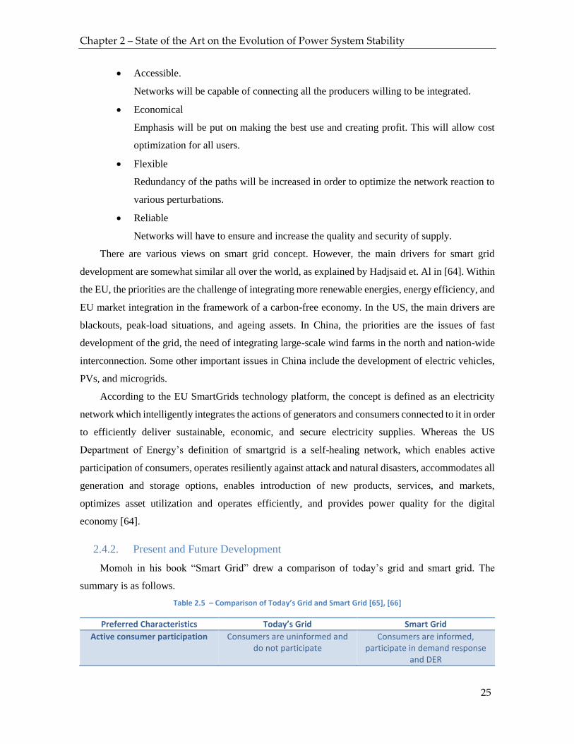
Chapter 2 – State of the Art on the Evolution of Power System Stability
25
Accessible.
Networks will be capable of connecting all the producers willing to be integrated.
Economical
Emphasis will be put on making the best use and creating profit. This will allow cost
optimization for all users.
Flexible
Redundancy of the paths will be increased in order to optimize the network reaction to
various perturbations.
Reliable
Networks will have to ensure and increase the quality and security of supply.
There are various views on smart grid concept. However, the main drivers for smart grid
development are somewhat similar all over the world, as explained by Hadjsaid et. Al in [64]. Within
the EU, the priorities are the challenge of integrating more renewable energies, energy efficiency, and
EU market integration in the framework of a carbon-free economy. In the US, the main drivers are
blackouts, peak-load situations, and ageing assets. In China, the priorities are the issues of fast
development of the grid, the need of integrating large-scale wind farms in the north and nation-wide
interconnection. Some other important issues in China include the development of electric vehicles,
PVs, and microgrids.
According to the EU SmartGrids technology platform, the concept is defined as an electricity
network which intelligently integrates the actions of generators and consumers connected to it in order
to efficiently deliver sustainable, economic, and secure electricity supplies. Whereas the US
Department of Energy’s definition of smartgrid is a self-healing network, which enables active
participation of consumers, operates resiliently against attack and natural disasters, accommodates all
generation and storage options, enables introduction of new products, services, and markets,
optimizes asset utilization and operates efficiently, and provides power quality for the digital
economy [64].
2.4.2. Present and Future Development
Momoh in his book “Smart Grid” drew a comparison of today’s grid and smart grid. The
summary is as follows.
Table 2.5 – Comparison of Today’s Grid and Smart Grid [65], [66]
Preferred Characteristics Today’s Grid Smart Grid
Active consumer participation Consumers are uninformed and do not participate
Consumers are informed, participate in demand response
and DER
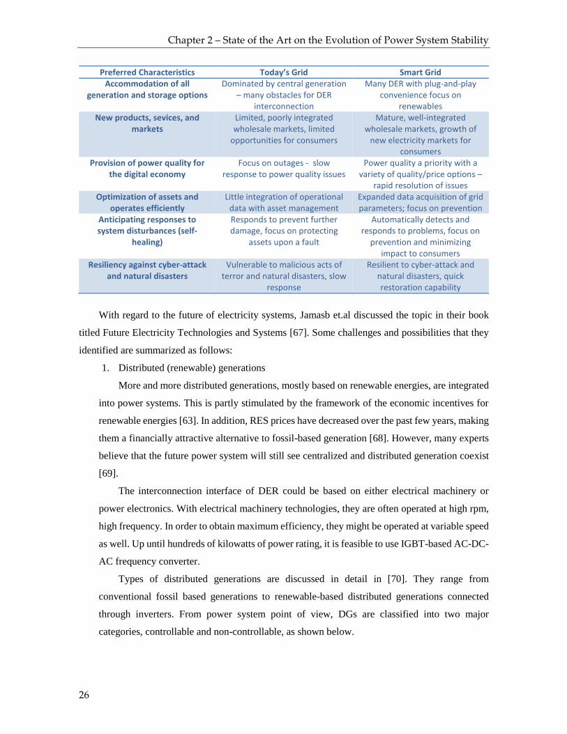
Chapter 2 – State of the Art on the Evolution of Power System Stability
26
Preferred Characteristics Today’s Grid Smart Grid Accommodation of all
generation and storage options Dominated by central generation
– many obstacles for DER interconnection
Many DER with plug-and-play convenience focus on
renewables New products, sevices, and
markets Limited, poorly integrated wholesale markets, limited
opportunities for consumers
Mature, well-integrated wholesale markets, growth of
new electricity markets for consumers
Provision of power quality for the digital economy
Focus on outages - slow response to power quality issues
Power quality a priority with a variety of quality/price options –
rapid resolution of issues Optimization of assets and
operates efficiently Little integration of operational
data with asset management Expanded data acquisition of grid parameters; focus on prevention
Anticipating responses to system disturbances (self-
healing)
Responds to prevent further damage, focus on protecting
assets upon a fault
Automatically detects and responds to problems, focus on
prevention and minimizing impact to consumers
Resiliency against cyber-attack and natural disasters
Vulnerable to malicious acts of terror and natural disasters, slow
response
Resilient to cyber-attack and natural disasters, quick restoration capability
With regard to the future of electricity systems, Jamasb et.al discussed the topic in their book
titled Future Electricity Technologies and Systems [67]. Some challenges and possibilities that they
identified are summarized as follows:
1. Distributed (renewable) generations
More and more distributed generations, mostly based on renewable energies, are integrated
into power systems. This is partly stimulated by the framework of the economic incentives for
renewable energies [63]. In addition, RES prices have decreased over the past few years, making
them a financially attractive alternative to fossil-based generation [68]. However, many experts
believe that the future power system will still see centralized and distributed generation coexist
[69].
The interconnection interface of DER could be based on either electrical machinery or
power electronics. With electrical machinery technologies, they are often operated at high rpm,
high frequency. In order to obtain maximum efficiency, they might be operated at variable speed
as well. Up until hundreds of kilowatts of power rating, it is feasible to use IGBT-based AC-DC-
AC frequency converter.
Types of distributed generations are discussed in detail in [70]. They range from
conventional fossil based generations to renewable-based distributed generations connected
through inverters. From power system point of view, DGs are classified into two major
categories, controllable and non-controllable, as shown below.

Chapter 2 – State of the Art on the Evolution of Power System Stability
27
Table 2.6 – Classifications of DGs [70]
DG Technology Controllable Non-Controllable
Conventional Fossil-Based Generation ✓
Microturbines ✓
Combined Heat and Power (CHP Plants) ✓
Small Hydro Power Plants ✓
Wind Turbines ✓
Photovoltaics ✓
Fuel Cells ✓
Geothermal Power Plants ✓
Biomass Power Plants ✓
Tidal Power Plants ✓
Wave Power Plants ✓
A significant portion of distributed generations is intermittent and interconnected through
inverters. They have different limitations and behavior from the classical synchronous machine-
based sources. The modeling and control strategies may vary from one manufacturer to the
others. However, they also offer more flexibility and faster response which could be the key to
the future grid operation. The flexibility includes dynamic variation of control parameters and
control algorithms, often under strict limitations of current and temperature.
Many studies considered that frequency variation is a consequence of a step variation of
power or production [71]–[73]. However, active power of renewable energy may fluctuate rather
slowly, as discussed in [74].
2. Limitations of semiconductors.
Voltage and current limits are regulated by the maximum allowable temperature. However,
due to the small unit scale of power electronics, there is no usable short time rating. As a future
perspective, silicon carbide devices will increase the ability of converters to withstand very high
currents in the future.

Chapter 2 – State of the Art on the Evolution of Power System Stability
28
3. Growth of microgrids
An important difference of a microgrid and a small power system is that microgrids may be
dominated by IBGs, therefore the operation and protection must be suited to power electronic
technologies.
4. Reactive compensation service from power electronics.
Basic hardware blocks used in all power electronics (PE) technologies are similar to each
other. The power processing can use the spare capacity of the inverter that is available when the
DG is not running at full power to provide reactive power compensation.
5. Compatibility level and load management [75]
Most domestic loads operate at low voltage DC, which normally include internal voltage
regulation that can tolerate considerable deviations in the voltage and the frequency supplied by
the utility. An increasing number of portable appliances, such as laptop and smartphone are
labelled “universal input”, indicating a wide range of operation, typically between 40 and 65 Hz
and 90 and 250 V. Two issues can be identified: first, an increasing number of loads belong to
the constant power type, consequently they consume a fixed power irrespective (within a certain
range) of the voltage and the frequency supplied. Constant-power loads deteriorate the damping
in a power system and may cause problems for system operators. Secondly, in terms of
compatibility, these loads are immune to high degrees of undervoltage and sag.
In systems other than public electricity supply, voltage regulation is treated differently.
Instead of regulating the distributed voltage to maintain tight limits, wide limits are authorized.
Reliance is then placed on the load-side, in the form of load regulation so as to process the
distribution voltage into a well-regulated voltage required for final use. The distribution inside a
computer system is designed based on this principle. The systems proposed for future
automobiles and electric aircraft also feature this philosophy of voltage regulation, and the same
philosophy can potentially be adapted for off-grid systems.
Newer standards and regulations show that more flexible voltage and frequency limits are
accepted. This is reflected in the evolution and amendment of IEEE 1547 standard. It was first
introduced in 2003 [76], and have been amended several times since then. It was originally
developed with an assumption of a lower penetration of DER, therefore it was rather specific to
grid-connected sources. However, the growth of DER has been very rapid since the inception of
the standard and the need for updating the standard is inevitable [77]. This standard, which will
be more thoroughly discussed in Subchapter 2.4.5, displays the acceptance of wider frequency
and voltage variations.
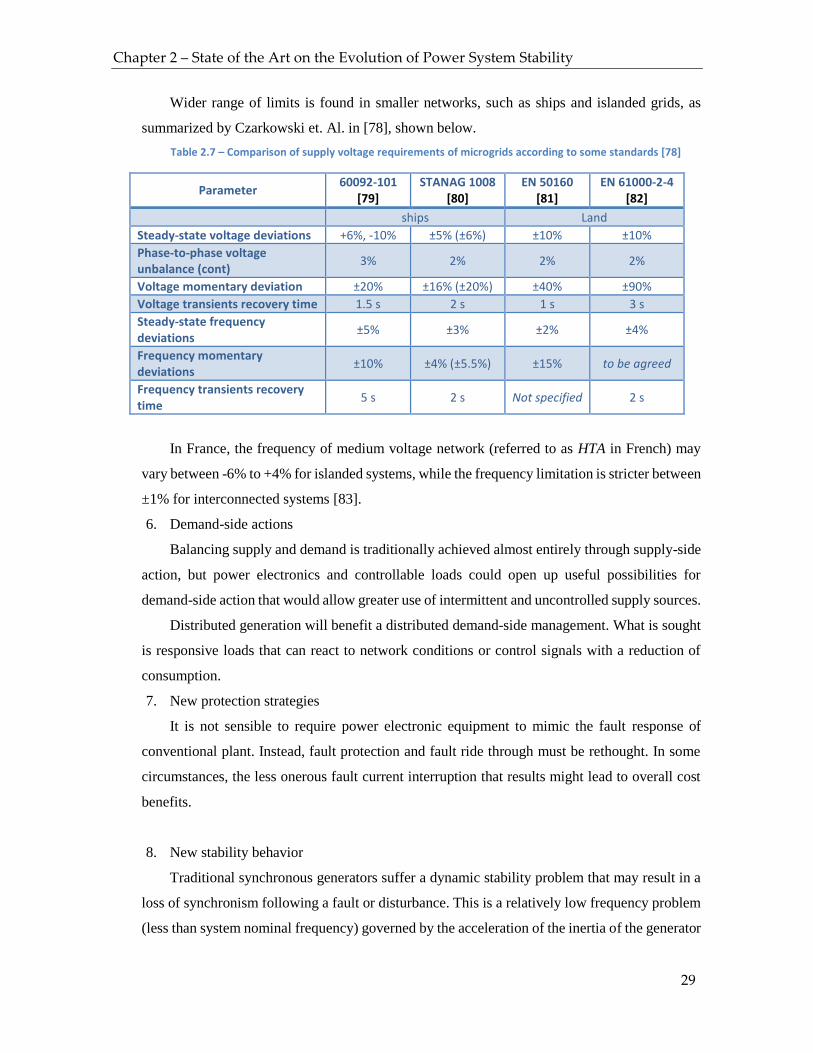
Chapter 2 – State of the Art on the Evolution of Power System Stability
29
Wider range of limits is found in smaller networks, such as ships and islanded grids, as
summarized by Czarkowski et. Al. in [78], shown below.
Table 2.7 – Comparison of supply voltage requirements of microgrids according to some standards [78]
Parameter 60092-101
[79] STANAG 1008
[80] EN 50160
[81] EN 61000-2-4
[82]
ships Land
Steady-state voltage deviations +6%, -10% ±5% (±6%) ±10% ±10%
Phase-to-phase voltage unbalance (cont)
3% 2% 2% 2%
Voltage momentary deviation ±20% ±16% (±20%) ±40% ±90%
Voltage transients recovery time 1.5 s 2 s 1 s 3 s
Steady-state frequency deviations
±5% ±3% ±2% ±4%
Frequency momentary deviations
±10% ±4% (±5.5%) ±15% to be agreed
Frequency transients recovery time
5 s 2 s Not specified 2 s
In France, the frequency of medium voltage network (referred to as HTA in French) may
vary between -6% to +4% for islanded systems, while the frequency limitation is stricter between
±1% for interconnected systems [83].
6. Demand-side actions
Balancing supply and demand is traditionally achieved almost entirely through supply-side
action, but power electronics and controllable loads could open up useful possibilities for
demand-side action that would allow greater use of intermittent and uncontrolled supply sources.
Distributed generation will benefit a distributed demand-side management. What is sought
is responsive loads that can react to network conditions or control signals with a reduction of
consumption.
7. New protection strategies
It is not sensible to require power electronic equipment to mimic the fault response of
conventional plant. Instead, fault protection and fault ride through must be rethought. In some
circumstances, the less onerous fault current interruption that results might lead to overall cost
benefits.
8. New stability behavior
Traditional synchronous generators suffer a dynamic stability problem that may result in a
loss of synchronism following a fault or disturbance. This is a relatively low frequency problem
(less than system nominal frequency) governed by the acceleration of the inertia of the generator
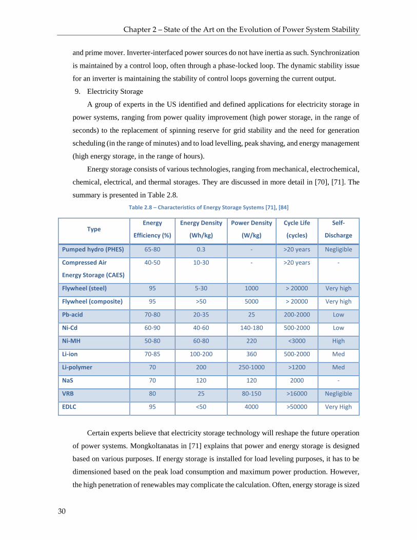
Chapter 2 – State of the Art on the Evolution of Power System Stability
30
and prime mover. Inverter-interfaced power sources do not have inertia as such. Synchronization
is maintained by a control loop, often through a phase-locked loop. The dynamic stability issue
for an inverter is maintaining the stability of control loops governing the current output.
9. Electricity Storage
A group of experts in the US identified and defined applications for electricity storage in
power systems, ranging from power quality improvement (high power storage, in the range of
seconds) to the replacement of spinning reserve for grid stability and the need for generation
scheduling (in the range of minutes) and to load levelling, peak shaving, and energy management
(high energy storage, in the range of hours).
Energy storage consists of various technologies, ranging from mechanical, electrochemical,
chemical, electrical, and thermal storages. They are discussed in more detail in [70], [71]. The
summary is presented in Table 2.8.
Table 2.8 – Characteristics of Energy Storage Systems [71], [84]
Type Energy
Efficiency (%)
Energy Density
(Wh/kg)
Power Density
(W/kg)
Cycle Life
(cycles)
Self-
Discharge
Pumped hydro (PHES) 65-80 0.3 - >20 years Negligible
Compressed Air
Energy Storage (CAES)
40-50 10-30 - >20 years -
Flywheel (steel) 95 5-30 1000 > 20000 Very high
Flywheel (composite) 95 >50 5000 > 20000 Very high
Pb-acid 70-80 20-35 25 200-2000 Low
Ni-Cd 60-90 40-60 140-180 500-2000 Low
Ni-MH 50-80 60-80 220 <3000 High
Li-ion 70-85 100-200 360 500-2000 Med
Li-polymer 70 200 250-1000 >1200 Med
NaS 70 120 120 2000 -
VRB 80 25 80-150 >16000 Negligible
EDLC 95 <50 4000 >50000 Very High
Certain experts believe that electricity storage technology will reshape the future operation
of power systems. Mongkoltanatas in [71] explains that power and energy storage is designed
based on various purposes. If energy storage is installed for load leveling purposes, it has to be
dimensioned based on the peak load consumption and maximum power production. However,
the high penetration of renewables may complicate the calculation. Often, energy storage is sized

Chapter 2 – State of the Art on the Evolution of Power System Stability
31
according to the penetration rate of variable renewables. If all energy production comes from
variable renewables, the energy storage may have to be designed according to the capacity of
the grid, which causes the project cost to skyrocket.
Despite countless research efforts dedicated into figuring the shape of the power system of the
future, it is still not very clear. Some of the possible scenarios identified by NREL from several
projects and reports are illustrated in Figure 2.9. In the figure, the names represent the examples in
progress and the institutions. It should be anticipated that the power systems will become increasingly
heterogeneous in the future.
Figure 2.9 – Scenarios for Emerging Power Systems [85]
2.4.3. The need for Flexibility
A power system is said to be flexible if it can, within economic boundaries, respond rapidly to
large fluctuations in demand and supply, both scheduled and unforeseen events, ramping down
production when demand decreases, and ramping up when it rises [86]. In terms of variable
renewables, a flexible system is the one capable of both absorbing large quantities of VRES and
disposing the surplus in a cost-effective way.
Power system flexibility can be obtained from a number of factors. On the supply side, the
resources include rapidly dispatchable power plants, interconnections, and energy storage systems.

Chapter 2 – State of the Art on the Evolution of Power System Stability
32
In addition, a significant flexibility resource is also accessible on the demand side: demand response
to deal with the power fluctuations. This is still somewhat under-exploited.
Electricity generation technologies include both dispatchable and variable types. Dispatchable
technologies are ones which can be relied on to supply electricity as required, except for special cases
such as technical or non-technical failures. Some renewable-based technologies belonging to this
classification include reservoir hydropower, biomass, geothermal, and some concentrating solar
thermal plants.
Variable renewable power plants depend on resources which fluctuate on the timescale of
seconds to days, and do not include any integrated storage. Technologies such as PV, wind power,
run-of-river hydropower, wave and tidal power belong to this category. It should be noted that the
output from such plants fluctuates according to the main renewable resource. Such technologies are
often referred to as intermittent, but the term variable is more representative since the output does not
drop from full power to zero or vice versa, but it rather ramps up or down as the weather systems
shift.
Flexibility is an intrinsic feature of interconnected networks. Electricity grids have an inherent
tolerance as actual operating conditions may depart from the assumptions made by planning
engineers. Flexibility assessment is not yet a common practice. Some TSO and DSO are pushing the
growth of VRES with a learning-as-we-go approach. A very simplified approach is suggested in [86]
to provide a broad picture of the factors. The first step is to identify the flexibility resource. The scale
of the existing, available resource of a power system depends on how it has evolved over time. Several
main sources of flexibility are as follows:
The quantity of fast response capacity in the generation portfolio
Storage availability: capacity and duration
Demand side management (DSM) response: the potential of consumers to alter their
electricity use in response to supply abundance/shortage.
Experience in Denmark shows that at times of high wind energy production, the electricity price
falls significantly. If low price periods can be capitalized by consumers, for example by shifting their
demand to such periods, the need for peaking plants can be reduced, and when it is high, the need for
storage systems or power export can be minimized. The second step is to take into account the existing
requirements for flexibility, such as existing balancing needs, errors in demand forecast, and
contingencies. The last step is to pay attention to the net flexible resource. If the targeted amount of
VRE generation exceeds what is possibly accommodated by the net flexibility resource, additional
measures must be taken to avoid power system stability problems.
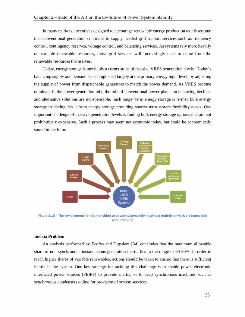
Chapter 2 – State of the Art on the Evolution of Power System Stability
33
In many markets, incentives designed to encourage renewable energy production tacitly assume
that conventional generation continues to supply needed grid support services such as frequency
control, contingency reserves, voltage control, and balancing services. As systems rely more heavily
on variable renewable resources, those grid services will increasingly need to come from the
renewable resources themselves.
Today, energy storage is inevitably a corner stone of massive VRES penetration levels. Today’s
balancing supply and demand is accomplished largely at the primary energy input level, by adjusting
the supply of power from dispatchable generators to match the power demand. As VRES become
dominant in the power generation mix, the role of conventional power plants on balancing declines
and alternative solutions are indispensable. Such longer term energy storage is termed bulk energy
storage to distinguish it from energy storage providing shorter-term system flexibility needs. One
important challenge of massive penetration levels is finding bulk energy storage options that are not
prohibitively expensive. Such a process may seem not economic today, but could be economically
sound in the future.
Figure 2.10 – The key elements for the transition to power systems relying almost entirely on variable renewable resources [87]
Inertia Problem
An analysis performed by Ecofys and Digsilent [34] concludes that the maximum allowable
share of non-synchronous instantaneous generation inertia lies in the range of 60-80%. In order to
reach higher shares of variable renewables, actions should be taken to ensure that there is sufficient
inertia in the system. One key strategy for tackling this challenge is to enable power electronic
interfaced power sources (PEIPS) to provide inertia, or to keep synchronous machines such as
synchronous condensers online for provision of system services.

Chapter 2 – State of the Art on the Evolution of Power System Stability
34
Synchronous condensers’ spinning rotor’s inertia, which makes the machines more tolerant of
grid disturbances, is exactly their key advantage over power electronic devices such as static VAR
compensators. New synchronous condensers remain 10-20% more costly per VAR of reactive power
capacity than an SVC [86]. But repurposing old power-plant generators upon decommissioning and
transforming those to synchronous condensers can be a quick and cheap solution. For example, gas
fired-power plants can now be equipped with clutches that decouple the turbines and generators,
allowing the machines to work as condensers. Another wild card is to absorb some power from the
wind turbines’ rotating mass. This is a strategy that could be used in the future to tackle the inertia
challenge.
2.4.4. Components
2.4.4.1. General Components and ICTs
Power grids were designed around conventional elements such as electrical machinery (rotating
machines, transformers), distribution lines, and loads. Those elements are the heart of a power grid.
A number of more intelligent elements are being integrated into power systems. They include smart
or communicating meters, actuators, fast switching devices, powerful sensors, and advanced
functions of network supervision and control, and batteries.
ICTs for power grids exist as embedded software, whether at the level of components or control
centers, and means of physical communications [64]. A particular interest is associated with the
following functions:
The smart meter with its different variants: broadband bidirectional communication,
possibility of load control tools and energy service
Advanced devices for energy management, either linked to smart meters or extension of
ADSL potentials
The intelligence associated with various domestic, tertiary, or industrial consumption
components. The typical example is decentralized and intelligent load-shedding based
on the grid frequency or voltage
Observability and supervisory control and network management linked with electricity
production and consumption
The intelligence carried by devices in the electrical network characterizing the following
process: measure, analyze, decide, act, and communicate. It is the main concern of the
whole distribution automation.
2.4.4.2. Load

Chapter 2 – State of the Art on the Evolution of Power System Stability
35
A wide variety of loads are supplied by a power system, such as electrical motors (pumps,
compressors), heating, lighting, and electronics, which may be controllable or not. They must be
appropriately modeled in power system studies. Improper load modeling may lead to an erroneous
conclusion of a study, as discussed in [88], [89]. Some load models are compiled in Table 2.9 from
the literature review. Special care also should be taken to parameter choice. Incorrect parameters may
also lead to incorrect results.
It should be noted that there is an important difference between static loads and dynamic loads.
Static loads are more suitable for static studies such as load flow analysis. The model is suitable for
steady state, where the dynamics following frequency and voltage changes are not the main focus.
On the other hand, dynamic load models can capture the behavior of a load following frequency and
voltage changes, including the phenomena of load rebounding and delays.
Table 2.9 – Summary of load modelling [88], [90]–[93]
Voltage Dependency
Frequency Dependency
General Characteris
tics
P =
f°(
V)
Q =
f°(
V)
P =
f°(
f)
Q =
f°(
f)
Mo
del
Sim
plic
ity
Kn
ow
led
ge
of
the
pa
ram
eter
s
Stat
ic L
oad
ZIP ✓ ✓ ✗ ✗ ✓
4 par. ✓
Exponential ✓ ✓ ✓ ✓ ✓
4 par. ✓
RLC ✓ ✓ ✗ ✓ ✓
1 par. ~+
RLC + RC ✓ ✓ ✓ ✓ ✓
3 par. ~-
Dyn
amic
Lo
ad M
od
els
(bla
ck b
ox)
Modified Exponential
✓ ✓ ✓ ✓ ~
7-8 par.
✓
Mod. Exponential + Cap (CRIEPI)
✓ ✓ ✓ ✓ ~
8-9 par.
✓
General Load Model (Power Factory)
✓ ✓ ✓ ✓ ✓
4-17 par.
✓

Chapter 2 – State of the Art on the Evolution of Power System Stability
36
It is noteworthy that the number of parameters relate to the number of parameters of the load
model (excluding P0 and Q0). Here, the general load model is discussed more thoroughly. This model
is often used throughout the thesis because of its flexibility, simplicity, suitability for static and
dynamic analyses, knowledge of parameters, and the availability in the chosen software program. The
discussion on other load models and their comparison can be found in [88].
Power factory’s general load model is a highly flexible model. The classical ZIP model, the
exponential model, and the modified exponential model are all specific cases of the general load
model. The model is depicted in the Figure and Equations below.
ΔfKpf + s·tpf
1 + s·t1
Kqf + s·tqf
1 + s·t1
1
1
Δu1 + s·
1 + s·t1
1 + s·t1
1
1
+
+
++
+
+
++
x
x
p1·Vkpu0 + p2·Vkpu1 + p3·Vkpu
q1·Vkqu0 + q2·Vkqu1 + q3·Vkqu
P
Q
P0
Q0
tpu/kput
1 + s·tqu/kqut
Figure 2.11 – Power Factory’s General Load Model to approximate the behavior of non-linear dynamic loads [92]
Where:
P, Q = Active power, reactive power
P0, Q0 = Active power, reactive power at nominal voltage
V = Voltage in per unit
p1, p2, p3 = coefficients of voltage dependency for active power
kpu0, kpu1, kpu = exponential coefficients of voltage dependency for active power
q1, q2, q3 = coefficients of voltage dependency for reactive power
kqu0, kqu1, kqu = exponential coefficients of voltage dependency for reactive power
Kpf, Kqf = coefficient of frequency dependency for active power and reactive power
Δu = voltage deviation in per unit
Δf = frequency deviation in per unit

Chapter 2 – State of the Art on the Evolution of Power System Stability
37
The sum of p1, p2, and p3 must be equal to 1. The same applies for the sum of q1, q2, and q3.
ZIP model has a long history of being employed in power system studies. The classical equations
are shown as follows [29].
𝑃 = 𝑃0 [𝑝1 + 𝑝2𝑉 + 𝑝3𝑉2](1 + 𝐾𝑝𝑓∆𝑓) Eq. 2.4
𝑄 = 𝑄0 [𝑞1 + 𝑞2𝑉 + 𝑞3𝑉2](1 + 𝐾𝑞𝑓∆𝑓) Eq. 2.5
This particular model has an important drawback. Frequency dependency is not represented.
This may be acceptable for load flow studies or for dynamic studies on stiff grids since the deviation
of frequency is very minor. Considering that the grid inertia is decreasing and more frequent load
imbalance might occur due to intermittent sources, frequency becomes an important factor to take
into account in load modeling. Here, the modified ZIP model seems convenient and promising. The
model takes frequency dependence and load dynamics into consideration. It is worth mentioning that
this model is also a particular case of power factory’s general load model.
ΔfKpf
1 + s t1
Kqf
1 + s t1
1
1
Δu1
1 + s t1
1
1 + s t1
1
1
+
+
++
+
+
++
x
x
p1 + p2 V + p3 V2
q1 + q2 V + q3 V2
P
Q
P0
Q0
Figure 2.12 – Power Factory’s General Load Model to approximate the behavior of non-linear dynamic loads [94]
The variables p1, p2, p3 as well as q1, q2, and q3 may be either positive or negative. This is useful
in defining the models which may have zero active or reactive power at nominal operating conditions
but may absorb power under frequency or voltage excursion.
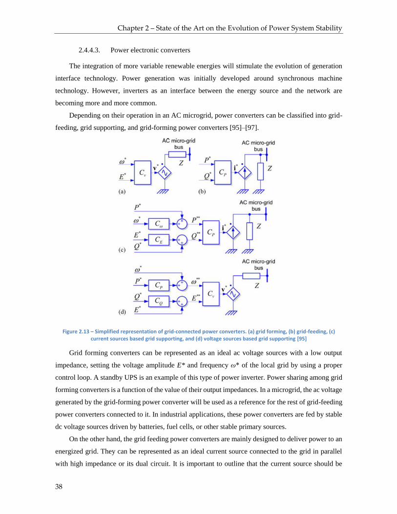
Chapter 2 – State of the Art on the Evolution of Power System Stability
38
2.4.4.3. Power electronic converters
The integration of more variable renewable energies will stimulate the evolution of generation
interface technology. Power generation was initially developed around synchronous machine
technology. However, inverters as an interface between the energy source and the network are
becoming more and more common.
Depending on their operation in an AC microgrid, power converters can be classified into grid-
feeding, grid supporting, and grid-forming power converters [95]–[97].
Figure 2.13 – Simplified representation of grid-connected power converters. (a) grid forming, (b) grid-feeding, (c) current sources based grid supporting, and (d) voltage sources based grid supporting [95]
Grid forming converters can be represented as an ideal ac voltage sources with a low output
impedance, setting the voltage amplitude E* and frequency ω* of the local grid by using a proper
control loop. A standby UPS is an example of this type of power inverter. Power sharing among grid
forming converters is a function of the value of their output impedances. In a microgrid, the ac voltage
generated by the grid-forming power converter will be used as a reference for the rest of grid-feeding
power converters connected to it. In industrial applications, these power converters are fed by stable
dc voltage sources driven by batteries, fuel cells, or other stable primary sources.
On the other hand, the grid feeding power converters are mainly designed to deliver power to an
energized grid. They can be represented as an ideal current source connected to the grid in parallel
with high impedance or its dual circuit. It is important to outline that the current source should be

Chapter 2 – State of the Art on the Evolution of Power System Stability
39
perfectly synchronized with the AC voltage at the connection point, in order to regulate accurately
the active and reactive power exchanged with the grid.
Grid feeding power converters are controlled current sources, presenting high parallel output
impedance. These converters are suitable to operate in parallel with other grid feeding power
converters in grid connected mode. Currently, most of the power converters belonging to DG systems
operate in grid-feeding mode, like PV and wind systems. However, they can participate in the control
of the microgrid ac voltage amplitude and frequency by adjusting the references of active and reactive
powers to be delivered.
Finally, the grid supporting converters can be represented either as an ideal ac-controlled current
source in parallel with a shunt impedance, or as an ideal ac voltage sources in series with a link
impedance. These converters regulate their output current/voltage to keep the value of the grid
frequency and voltage amplitude close to their rated values.
The main objective of grid supporting power converter is to deliver proper values of active and
reactive power to contribute to the regulation of the grid frequency and the voltage. A grid supporting
power converter is controlled as a voltage source with a link-impedance, or alternatively, as a current
source with a parallel impedance. In any case, its main objective is to participate in the regulation of
the ac grid voltage amplitude E* and frequency ω* by controlling the active and reactive power
delivered to the grid. An example of this type of power inverter is line-interactive UPS systems.
2.4.5. Regulation and Standards
2.4.5.1. Regulation
The frequency regulations are typically classified as follows [29], [40], [71], [98].
1. primary regulation (0 – 10s)
Sometimes it is referred to as the frequency containment process. The objective is to
stabilize the frequency after a disturbance at a steady state value within the permissible maximum
steady state frequency deviation by a joint action of frequency containment resources within the
system.
The frequency responsive spinning reserve is responsible for this function. It is comprised
of online synchronous machines controlled by speed droops. According to a study on change
proposals to the grid codes in England & Wales and in Scotland [99], the characteristic reduction
in the network demand due to frequency fall of typically 2% per Hz may be taken into account
as a part of operating reserves in primary regulation.

Chapter 2 – State of the Art on the Evolution of Power System Stability
40
During the first 10 seconds, it is possible that the frequency drops below the permissible
value, and this consequently can trigger the automatic load shedding scheme.
2. secondary regulation (~10s – 10 minutes)
It is also referred to as the frequency restoration process. It controls the frequency towards
its nominal value by the activation of frequency restoration reserve and replaces the activated
frequency containment reserve. This process can be performed either automatically or manually.
All spinning reserve capable of changing the power output immediately, as well as offline
generators capable of being synchronized within 10 minutes is responsible for this function.
Sometimes it requires manipulation of the speed/load reference.
3. Tertiary regulation (>10 min)
It is sometimes referred to as the reserve replacement process. It replaces the activated
frequency restoration reserve (FRR) and/or supports FRR activation by activation of the reserve
replacement. Reserve replacement is comprised of all generators having the response speed on
the time scale of more than 10 minutes. Tertiary regulation is sometimes not necessary,
depending on the severity of the fault.
According to Indonesian Grid Codes [100]–[103], some supplementary actions other than the
three frequency regulation strategies may be taken when necessary. They are as follows:
1. Manual dispatching command to power plants
2. Voltage set point reduction (also known as brown-out) to reduce active power demand
3. Manual load shedding
4. Automatic load shedding (with underfrequency relays)
5. Generator tripping by overfrequency relays
Similar to frequency regulations, there exist also some regulation strategies concerning the
voltage stability, as presented below [104]:
1. Primary voltage regulation (0 – 10s)
The primary voltage regulation (PVR) is performed by automatic and rapid voltage
regulators which control reactive power output so that the output voltage magnitudes are kept at
specified values. PVR has only local scope targeting the control in the particular bus assigned to
the controllable device. Generally, the primary voltage control is performed by the generator’s
automatic voltage regulator (AVR). The AVR regulates the voltage by controlling the excitation
system. The other controllable devices such as synchronous condenser, SVC, and STATCOM
can also be used for PVR.
2. Secondary voltage regulation (~10s – 10 minutes)

Chapter 2 – State of the Art on the Evolution of Power System Stability
41
The coordination and the supervision of the PVR set point values within a given
geographical zone are the tasks of the secondary voltage regulation (SVR). The main idea behind
SVR is to coordinate the various regional reactive power resources in such a manner that they
control the voltage at given pilot nodes. Pilot nodes are selected such that the voltage magnitude
at the pilot node represents the voltage profile over the associated zone. Another method for pilot
node selection is based on electrical distance concept between nodes.
3. Tertiary voltage regulation (>10 mins)
The basic idea behind the tertiary voltage regulation (TVR) is to increase the operating
security and efficiency of the system through a centralized coordination of the zonal SVR
structure. The TVR considers counteract coupling between controls at the SVR levels. In fact,
TVR defines the optimal voltage points for the SVR pilot nodes.
Regulation in Microgrids
The frequency and voltage regulations in microgrids marked by high level of power electronics
are classified as follows [95]. This regulation is also applicable to microgrids, where different DG
technologies form various primary resources (oil, gas, wind, sun, tide, water, etc.) and with a broad
variety of roles (grid-feeding, grid-supporting, and grid-forming) may be interconnected.
1. The primary control level
Also known as local control, it allows multiple actors to work together with the aim of
maintaining local variables such as voltage, frequency, or current injection within the accepted
range. A vital feature of the primary control is to distribute the power injected into the microgrid
to each DG unit. The local controllers may include droop strategy and virtual impedance control
techniques available on each DG unit.
2. The secondary control level
It acts as a centralized automatic generation controller and compensates quasi-steady-state
errors. Under any voltage or frequency deviation, a secondary control action is applied to
multiple DG units in the microgrid to restore their nominal values, for example by adjusting the
droop characteristic coefficients or by changing the active power and reactive power references.
Compared with conventional generators, this secondary control has faster response, but limited
by some factors such as the battery ratings or the primary resource availability. This control uses
communications and wide-area monitoring systems to harmonize the actions of all generation
units within the power grid. The time response is in the range of minutes, which is slower
compared to primary control.
3. The tertiary control level

Chapter 2 – State of the Art on the Evolution of Power System Stability
42
It is in charge of the optimization of microgrid operation, normally based on economic
criteria, taking into consideration the generation cost, the demand and supply balance and its
short term forecast. It acts over the secondary control level with the objective to restore the
secondary control reserve, as well as to set the microgrid voltage and frequency to their nominal
values in case the secondary reserve is not effective enough.
2.4.5.2. Codes and Standards
Due to future challenges introduced by high penetration of power electronic interfaced sources,
normally employed for intermittent source interconnection, in 2017 ENTSO-E published a guidance
document for national implementation for network codes on grid connection [105]. This guidance
focuses on RES power sources interfaced via power electronics. Important aspects such as capabilities
to manage low total system inertia (TSI), low synchronizing torque, low short-circuit power, and low
dynamic voltage support are some problems that the guidance deals with. The guidance also identifies
stability challenges and potential remedial actions, including their side effects. The possible remedial
actions include costly conventional approaches (synchronous generators, synchronous
compensators), and the holistic approach in which the power electronic interfaced sources contribute
to system strength. Control strategies can be implemented into power electronics. Strategies such as
swing equation based inertial response and grid-forming control strategies. However, care should be
taken to ensure that delays in measurement and controls are carefully taken into account to avoid
adverse impact on system stability.
The same challenges also affected North American standards. As discussed in [77], [106]–[108],
IEEE 1547 standard which deals with DER of 10 MVA or less, and is technology neutral, has
undergone several important updates, as shown in Table 2.10.
Table 2.10 – History of IEEE 1547
Year Event
2003
IEEE 1547-2003 [76] (Standard for Interconnecting Distributed Resources with
Electrical Power Systems) was published as a voluntary industry standard. It was
originally developed with an assumption of a low penetration of DER. It provides
requirements regarding the performance, operation, testing, safety, and
maintenance of the interconnection, including general requirements, responses
to abnormal conditions, power quality, islanding, and test requirements.
2005
Energy Policy Act cites IEEE 1547 Standard as the best practice for
interconnection and it is adopted by all states.

Chapter 2 – State of the Art on the Evolution of Power System Stability
43
Year Event
IEEE 1547.1 [109] standard for conformance testing and evaluation was
approved.
2007
Energy Independence and Security Act cites IEEE as a standards development
organization partner to NIST and the lead to coordinate framework and
roadmap for Smart Grid Interoperability standards.
IEEE 1547 is adopted by the majority of jurisdictional entities across North
America that set DER interconnection rules.
IEEE 1547.3 [110] which addresses guidelines for monitoring, information
exchange, and control for DER interconnections was published.
2008 IEEE 1547.2 Standard [111] providing background on 1547 (version 2003)
requirements, tips, techniques, and rules of thumb was approved.
2011
IEEE Standard 1547.4 [112] providing approaches and good practice for the
design, operation, and integration of microgrids was approved and published.
IEEE Standard 1547.6 [113] for recommended practices that address spot and
grid distribution networks was published. It also provides solutions for the
interconnection of DER on distribution systems.
2013
Amendment 1 (IEEE 1547a [114]) was passed to voltage and frequency
regulation in December 2013 – the process to completely revise IEEE Standard
1547 began. IEEE Standard 1547.7 [115] addressing criteria, scope, and extent
for grid impact studies due to DER.
2014
Amandment 1 (IEEE Standard 1547a-2014) was adopted in May 2014. It
removed restrictions against DER from actively participating in grid voltage
regulation.
2017 IEEE 1547 full revision was balloted and approved
2018
IEEE Standard 1547-2018 [116] (revision of IEEE Standard 1547-2003) was
approved and published. Here, requirements and specifications of DER for
reactive power capability, voltage and frequency support, and ride through
capability, and performance when connected to an intentional island are
provided.
A comparison of applicable grid standards in North America from a technical point of view is
presented as follows [77].

Chapter 2 – State of the Art on the Evolution of Power System Stability
44
Table 2.11 – Comparison of North American Standards
Function
Set
Advanced Functions IEEE 1547-
2003
IEEE 1547a-
2014
IEEE 1547-
2018
CA Rule 21-
2015
Static Adjustable Trip Settings
Controlling Power Curtailment
Ramp Rate Control
Frequency
Support
L/H Frequency Ride Through
ROCOF Ride-Through
Frequency-Watt
Voltage
Support
L/G Voltage Ride Through (VRT)
Dynamic Voltage Support during
VRT
Voltage Phase Angle Jump Ride-
Through
Fixed power factor
Fixed reactive power
Volt-Var
Volt-Watt
Watt-Var
Legend: Prohibited, Allowed by mutual agreement, capability required
2.5. Microgrids
2.5.1. Introduction
Small isolated grids have existed for years in remote communities. However, the microgrid
concept was formally introduced in 2001 by Bob Lasseter as a concept to deal with distributed
renewable energy [117]. In general, microgrid is defined as an integrated energy system within clearly
defined electrical boundaries consisting of distributed energy resources and multiple electrical loads
operating as single, autonomous grid either in parallel to or islanded from the existing utility power
grid. However, The exact definition of microgrids varies in terms of size, capacity, components, and
behaviors [118]–[123].
Microgrid is often regarded as an important part of smart grid, since it offers enhancements to
power systems, notably in reliability, sustainability, and economic aspects. However, there are several
regional/national focuses regarding microgrid concept, as discussed in [124]. The US views microgrid
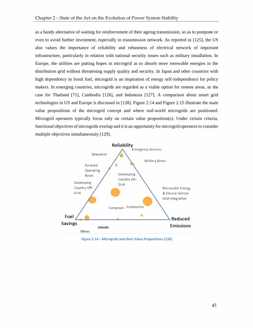
Chapter 2 – State of the Art on the Evolution of Power System Stability
45
as a handy alternative of waiting for reinforcement of their ageing transmission, so as to postpone or
even to avoid further investment, especially in transmission network. As reported in [125], the US
also values the importance of reliability and robustness of electrical network of important
infrastructure, particularly in relation with national security issues such as military installation. In
Europe, the utilities are putting hopes in microgrid as to absorb more renewable energies in the
distribution grid without threatening supply quality and security. In Japan and other countries with
high dependency in fossil fuel, microgrid is an inspiration of energy self-independence for policy
makers. In emerging countries, microgrids are regarded as a viable option for remote areas, as the
case for Thailand [71], Cambodia [126], and Indonesia [127]. A comparison about smart grid
technologies in US and Europe is discussed in [128]. Figure 2.14 and Figure 2.15 illustrate the main
value propositions of the microgrid concept and where real-world microgrids are positioned.
Microgrid operators typically focus only on certain value proposition(s). Under certain criteria,
functional objectives of microgrids overlap and it is an opportunity for microgrid operators to consider
multiple objectives simultaneously [129].
Figure 2.14 – Microgrids and their Value Propositions [130]
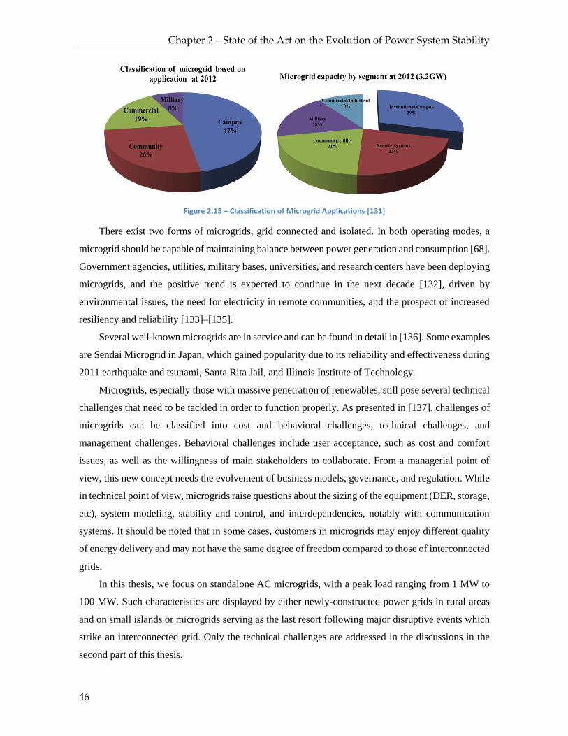
Chapter 2 – State of the Art on the Evolution of Power System Stability
46
Figure 2.15 – Classification of Microgrid Applications [131]
There exist two forms of microgrids, grid connected and isolated. In both operating modes, a
microgrid should be capable of maintaining balance between power generation and consumption [68].
Government agencies, utilities, military bases, universities, and research centers have been deploying
microgrids, and the positive trend is expected to continue in the next decade [132], driven by
environmental issues, the need for electricity in remote communities, and the prospect of increased
resiliency and reliability [133]–[135].
Several well-known microgrids are in service and can be found in detail in [136]. Some examples
are Sendai Microgrid in Japan, which gained popularity due to its reliability and effectiveness during
2011 earthquake and tsunami, Santa Rita Jail, and Illinois Institute of Technology.
Microgrids, especially those with massive penetration of renewables, still pose several technical
challenges that need to be tackled in order to function properly. As presented in [137], challenges of
microgrids can be classified into cost and behavioral challenges, technical challenges, and
management challenges. Behavioral challenges include user acceptance, such as cost and comfort
issues, as well as the willingness of main stakeholders to collaborate. From a managerial point of
view, this new concept needs the evolvement of business models, governance, and regulation. While
in technical point of view, microgrids raise questions about the sizing of the equipment (DER, storage,
etc), system modeling, stability and control, and interdependencies, notably with communication
systems. It should be noted that in some cases, customers in microgrids may enjoy different quality
of energy delivery and may not have the same degree of freedom compared to those of interconnected
grids.
In this thesis, we focus on standalone AC microgrids, with a peak load ranging from 1 MW to
100 MW. Such characteristics are displayed by either newly-constructed power grids in rural areas
and on small islands or microgrids serving as the last resort following major disruptive events which
strike an interconnected grid. Only the technical challenges are addressed in the discussions in the
second part of this thesis.

Chapter 2 – State of the Art on the Evolution of Power System Stability
47
Indonesia’s point of view
Romer et. Al. discussed the road map of smart grid development in Indonesia in [127]. One of
the most important challenges to tackle in the archipelago is how to supply more than 250 million
people with access to electricity. Other than the population growth which is expected to reach 300
million people in 15 years, the outlook of economic growth will lead to a heavy increase of electricity
demand. An additional challenge is how to bring energy access to all of Indonesian population,
considering the country’s geographic situation, where the inhabitants are spreading over 5000 islands.
Smart grid approaches are also necessary in order to efficiently achieve energy access for all, which
will push welfare creation. The optimal approach is a mixture between on-grid and off-grid solutions
depending on local characteristics. The grid should be made fit for renewable energies, which are
variable in most cases. The variability can be handled through approaches such as integrated storage
systems or demand side management mechanisms.
2.5.2. Stability Behavior
The definition of stability in microgrids and in conventional interconnected power systems is
principally based on the same principle. As stated in [68], a microgrid is considered stable if, after
being subjected to a perturbation, all state variables recover to (possibly new) steady state values
which satisfy operational constraints. And a microgrid should be considered stable if it fulfils its main
objective. For example, when a microgrid is constructed for supplying power to important loads and
it fails to do so, the microgrid is said to be unstable.
The nature of stability problem and dynamic power performance of a microgrid are different
from those of a conventional power system discussed previously in Section 2.2. The most important
distinguishing factors are identified in [50], [68], as follows:
1. Smaller system size
2. Higher penetration of (V)RES
3. Higher uncertainty in the system
4. Lower system inertia
5. Higher R/X ratio of the feeders, especially in low voltage
6. Low short circuit capacities
7. Relatively unbalanced three-phase loadings, especially for small community grids
The evolution of power system classification over time in the literature is illustrated in Figure
2.16.

Chapter 2 – State of the Art on the Evolution of Power System Stability
48
2004 IEEE/CIGRE classification
As discussed in Section 2.2, in order to facilitate power system stability analysis, IEEE/CIGRE
Joint Task Force [26] in 2004 classifies power system stability into three main categories: rotor angle
stability, frequency stability, and voltage stability. This classification is based on the structure of
conventional power systems, supplied mostly by dispatchable synchronous machines. Nevertheless,
it is mentioned in the document that in isolated island systems, frequency stability could be of concern
due to frequent imbalance between power generation and demand [26], [138].
Majumder’s classification
In 2013, Majumder pubished a journal article [122] which classifies microgrid stability into three
main categories: small signal stability, transient stability, and voltage stability. The classification does
not formally include frequency and angle stability although they are implicitly defined under small
signal and transient stability, as identified from the state variables.
Here, a microgrid is composed of synchronous generators, inverter-based DG, lines, electrical
machinery loads, and impedance loads. It may work in grid-connected or islanded modes. Small
signal stability is analyzed with linearized model. It is strongly associated with feedback controllers.
All state variables are used to derive state space models. Then, Eigen value analysis complimented
by time domain simulation can be used for the analysis. Transient stability is concerned with large
perturbations. It is analyzed with nonlinear model through the construction of the Lyapunov function
or time-domain simulation. It deals mostly with the protection strategy and the balance between
power generation and consumption. Voltage stability focuses more on load-side rather. It can be
demonstrated with the P-V and Q-V curves. It is strongly associated with current limiters, tap-
changers, and load regulations. The author identified that due to the much faster time response of
VSC with respect to synchronous machines, oscillation may exist if the control strategies are not
carefully chosen.
Shuai’s Classification
Shuai et. Al published a journal article devoted to microgrid stability classification [50] in 2016.
The authors considers that IBGs are the main power supply in a microgrid. Consequently, the dynamic
process is more complicated. They firstly classifies microgrid stability into two cases: grid connected
microgrid and islanded microgrid. Only the further classification under islanded microgrid category
is of interest in this discussion.
Here, islanded microgrid stability is classified into frequency stability and voltage stability. Both
are further classified into small disturbance stability and transient stability. With respect to the
classical classifications proposed by IEEE/CIGRE Joint Task Force in 2004, Shuai et. Al introduce
ultra-short term stability under transient stability cases for both voltage stability and frequency
Chapter 2 – State of the Art on the Evolution of Power System Stability
49
stability. This is due to the fact that the inrush current during a fault may be dangerous to inverters
and it happens in the time span of milliseconds. Furthermore, angle stability is not acknowledged as
a category.
2018 IEEE Classification
Recently, IEEE Task force issued a technical report draft in which they define a new
classification of microgrid stability [68]. This report has also been published as a journal article [139].
A number of differences in terms of stability issues in microgrids and in conventional interconnected
grids are identified. In isolated microgrids, maintaining frequency stability proves to be challenging
because of the low system inertia and high levels of VRES, contrary to the case of conventional
interconnected systems where angle and voltage stability problems occur more often. Problems such
as inter-area oscillations and voltage collapse have not been detected in isolated microgrids.
The new classification is based on partial stability concept, in which stability problems can be
classified according to the physical cause of instability, the relative size of the perturbation, the
physical components involed, the time-span during which the instability manifests itself, and the
methodology to analyze the instability. It firstly divides microgrid stability into two main categories:
power supply and balance stability and control system stability.
Power supply and balance deals with the ability of the system to maintain the power balance and
effective active and reactive power sharing among DGs. This category is furthermore subcategorized
into frequency and voltage stability. The task force also noticed that due to the higher R/X ratio in
microgrids, the decoupling of active power flow and voltage magnitude is not valid anymore.
Therefore, voltage-frequency stability coupling should be considered for stability analysis. With
respect to voltage stability, the task force observes with the current trend, the sensitivity of load power
consumption to voltage and DG current limits may be influential factors in microgrids. This may
result in unacceptable low steady-state and dynamic voltages. Besides system voltage stability, this
classification introduces DC-link voltage stability. Voltage ripples of the capacitor depend on the
instantaneous power of the inverter. When the power injection of the inverter is close to its limit,
undamped DC voltage ripples may occur, which will result in large fluctuations in the active and
reactive power output of DERs.
Control system stability issues may occur because of inadequate control schemes and/or poor
tuning of one or more controllers. This category is further split into electric machine and converter
stability. With respect to conventional interconnected systems, the issues of out of synchronism of
synchronous machines have not been observed in this classification. Electric machine stability in
microgrids is dominantly associated with poor tuning of the exciter and governor, which could result
in undamped oscillation and continuous increase/decrease of voltage and frequency. Converter

Chapter 2 – State of the Art on the Evolution of Power System Stability
50
stability issues are caused by poor controller tuning and the impact of the usage of phase-locked loop
(PLL). Synchronization stability problems linked with PLL performance are more pronounced in
weak grids, as discussed in [140]. PLL introduces negative parallel admittance to the input admittance
which may provoke instabilities. The choice of PLL bandwidth must be carefully taken. Higher
bandwidth introduces negative admittance, and low bandwidth may cause the PLL to fail to properly
detect zero crossings which deteriorates the synchronization process.

51
Power System
Stability
Frequency
Stability
Rotor Angle
Stability
Voltage
Stability
Small-Disturbance
Angle Stability
Transient
Stability
Short Term Short Term Long Term
Small-Disturbance
Voltage Stability
Large-Disturbance
Voltage Stability
Short Term Long Term
Ultra short
term
Ultra short
term
Small
Disturbance
Large
Disturbance
Power Supply
and Balance
Stability
Control System
Stability
Converter
Stability
Small DisturbanceLarge
Disturbance
Long TermShort Term
Electric
Machine
Stability
System Voltage
Stability
DC-Link Voltage
stability
Legend:
Small Signal
Stability
Transient
Stability
IEEE/CIGRE Task Force, 2004
Majumder, 2013Shuai, 2015
IEEE Task Force, 2018
Figure 2.16 – Stability Classifications in Microgrids in Literature

Chapter 2 – State of the Art on the Evolution of Power System Stability
52
Comments on Microgrid Stability Classification
In general, the stability classification proposed in 2018 IEEE classification accommodates the
results of this PhD research. It lays important emphasis on differentiating the stability issues due to
power balance and control problems. However, it is necessary to complement the explanations based
on the findings in this PhD research.
In line with 2018 IEEE Classification, this research discovered that in microgrids, stability
problems are classified into power balance stability and control stability. Power balance stability deals
with the law of energy conservation and covers frequency and voltage stability. It is concerned with
the capability of the ensemble of the network (including elements such as sources, transformers and
feeders) to deliver load demand. High excursions of frequency and voltage are common in microgrids.
Both variables are coupled due to and the higher R/X ratio, the behavior of grid forming elements
(i.e. frequency affects armature voltage for synchronous machines), and the behavior of loads (i.e.
active and reactive power demands are dependent on voltage and frequency). Power balance
instability may arise even when the power system has enough reserve to respond to power demand,
for example due to poor power sharing among sources or loadability limit. Control stability is
concerned with machine physical behavior, control strategies, their interaction, and their tuning. It is
divided into small signal stability and large perturbation stability. Instability often manifests itself as
undamped oscillations or uncontrolled hysteresis.
Contrary to Reference [68] which reported that loss of synchronism and voltage collapse have
not been observed in microgrids, this research found out that out-of-synchronism and voltage collapse
may still exist in microgrids as reported in [94], [141]. This conclusion is based on our study on a
typical isolated microgrid in Indonesia which is characterized by long distribution lines and
distributed synchronous machines, in contrast to microgrids reported in [68] which assume short
feeders.
Single point small signal stability might not be very useful as microgrid’s point of operation
changes constantly. However, it is important to verify small signal stability to guarantee power system
stability. Therefore, in this research, small signal analysis is conducted at the same time as transient
stability analysis. Time domain simulation is utilized to study both transient and small signal stability.
Stable non-oscillatory variables are ensured at the initialization and the post-perturbation state in
order to verify small signal stability.
PLL plays a very important role in the performance of a grid connected power converters. A
precise synchronization algorithm is needed to estimate the grid voltage parameters (voltage
amplitude, frequency, and phase angle) accurately. These values are crucial in controlling active and
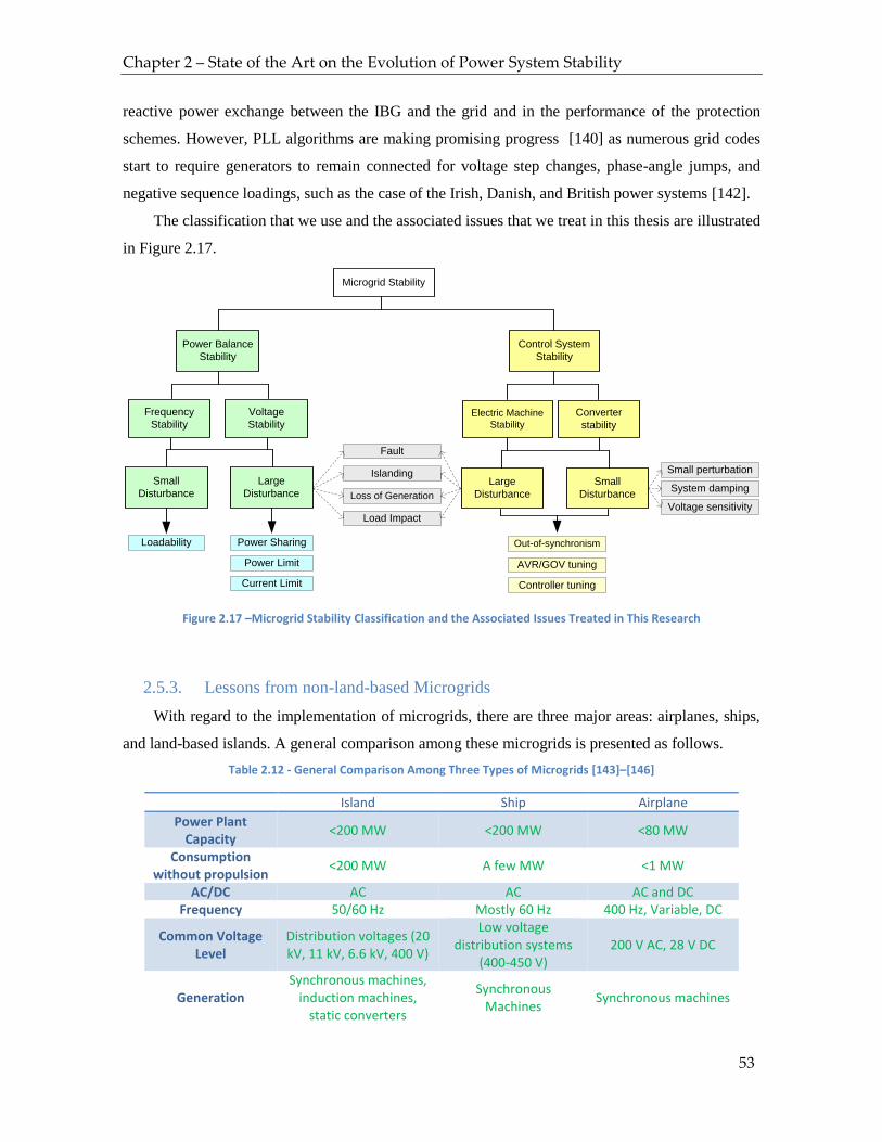
Chapter 2 – State of the Art on the Evolution of Power System Stability
53
reactive power exchange between the IBG and the grid and in the performance of the protection
schemes. However, PLL algorithms are making promising progress [140] as numerous grid codes
start to require generators to remain connected for voltage step changes, phase-angle jumps, and
negative sequence loadings, such as the case of the Irish, Danish, and British power systems [142].
The classification that we use and the associated issues that we treat in this thesis are illustrated
in Figure 2.17.
Microgrid Stability
Power Balance
Stability
Control System
Stability
Small
Disturbance
Large
Disturbance
Loadability
Current Limit
Power Limit AVR/GOV tuning
Controller tuning
Out-of-synchronism
System damping
Small perturbation
Voltage
Stability
Frequency
Stability
Power Sharing
Large
Disturbance
Small
Disturbance
Converter
stability
Electric Machine
Stability
Islanding
Fault
Load Impact
Loss of GenerationVoltage sensitivity
Figure 2.17 –Microgrid Stability Classification and the Associated Issues Treated in This Research
2.5.3. Lessons from non-land-based Microgrids
With regard to the implementation of microgrids, there are three major areas: airplanes, ships,
and land-based islands. A general comparison among these microgrids is presented as follows.
Table 2.12 - General Comparison Among Three Types of Microgrids [143]–[146]
Island Ship Airplane
Power Plant Capacity
<200 MW <200 MW <80 MW
Consumption without propulsion
<200 MW A few MW <1 MW
AC/DC AC AC AC and DC Frequency 50/60 Hz Mostly 60 Hz 400 Hz, Variable, DC
Common Voltage Level
Distribution voltages (20 kV, 11 kV, 6.6 kV, 400 V)
Low voltage distribution systems
(400-450 V) 200 V AC, 28 V DC
Generation Synchronous machines,
induction machines, static converters
Synchronous Machines
Synchronous machines

Chapter 2 – State of the Art on the Evolution of Power System Stability
54
Primary Energy Fossil (e.g. diesel, gas), renewables (hydro, PV,
wind) Diesel, nuclear Jet fuel (avtur)
Traditionally, the propulsion system and the power consumption are separated. However, with
movements towards more electric architectures for aircrafts and ships, there is a trend towards
integrated electric propulsion where a single set of generators provides electric power for both
propulsion and other loads aboard the ship. This transformation is driven by efficiency, survivability,
and the anticipated development of high powered sensors and weapons. This can furthermore result
in new frequency and voltage choices.
From such a comparison, several interesting points containing possible cross-fertilization,
especially between island microgrids and ship microgrids of comparable size, are summarized as
follows [143].
1. Design and operation
In electrical systems, load and generation must be balanced at all times. In microgrids, the
available generation is typically sized to provide continuous supply to critical loads. Therefore,
non-critical loads occasionally must be shed either manually or automatically, depending on their
system design and protection, in order to maintain the power balance. Demand response plays a
vital role in this matter.
In terrestrial microgrids, load shedding is typically triggered by under-frequency relays,
whereas load shedding in vessel power systems is based on power sensors which monitor
generator power output. When the demand exceeds a certain percentage of the generator rating
within a defined time delay, a predetermined load shedding scheme is triggered. An important
difference is that in land-based microgrids, the power provider and the customers are different
entities, hence negotiation with regard to load shedding is necessary. It is normally conducted in
advance, or else a complete shutdown may be inevitable. On ships, the entire system, including
the loads, belongs to the same entity, hence less negotiation for load shedding.
2. Generation
The generation system of both types of microgrids is sized to supply loads. In land-based
microgrids, the electricity may be generated by conventional generators or non-synchronous
generators (inverters, induction generator), either with renewable energy or fossil fuel as the
primary energy. Although there are many forms of generation for vessel systems, the most
common way to generate electric power is through gas turbines or diesel generators, working
collectively to supply both critical and non-critical loads.

Chapter 2 – State of the Art on the Evolution of Power System Stability
55
3. Load Types
The characteristics of loads in land-based microgrids are similar to those of the larger grids.
The difference manifests itself in the scale and numbers. In general, the following features can
be identified for loads in both types of microgrids: They tend to be conventional and have
comparable electrical characteristics; they tend to be continuous, typically varying on time scales
of minutes to hours, however some loads in future warships may have intermittent nature, such
as electric guns and weaponry; no single load is dominant, except propulsion loads for ships
(those may comprise 90% of the installed power capacity. However, propulsion can be controlled
accordingly so as not to severely impact the system’s stability); individual loads are typically
switched on and off in discrete increments, but their accumulation remains smooth and can be
modeled as a mildly varying function of time; total system load tends to be predictable based on
historical data.
4. Dynamic Balancing
Dynamic balancing is accomplished by adjusting generation set points and controlling non-
critical loads. However, non-critical load management on vessel systems may have an extra
complexity, because most of the loads are supplied through two redundant feeders.
5. Stability
Compared to terrestrial microgrids, ships may have a higher proportion of constant power
loads, which have destabilizing effects. Consequently, the design of practical stabilizing
strategies for ships becomes more demanding.
Boundary controllers can be applied in both types of microgrids. Boundary controllers
designed for electric ships provide faster dynamic responses than classical PID controllers. This
is also a desirable characteristic for land-based microgrids due to its capability to obtain fast
compensation following generation or load impacts.
It should be noted that the generation-side on ships is more controllable than that of land-
based microgrids. Therefore, both generation and load management can be exploited to deal with
frequency and voltage stability for ships. In land-based microgrids, both generation and load
management can also be utilized to maintain system stability. However, the options are rather
limited based on the agreement between multiple entities in the grid (i.e. DSO, customers,
generation) and the type of land-based microgrid (e.g. campus microgrid, islanded microgrids,
military base).
6. Autonomous operation and communication infrastructure
Locally available droop based schemes are commonly employed for power management
purposes within terrestrial microgrids. In contrast, a ship power system is conventionally

Chapter 2 – State of the Art on the Evolution of Power System Stability
56
designed in a centralized manner in order to obtain a high level of security and dependability. In
this application, the communication system is vital. Over the last decade, there has been a move
toward the widespread installation of smart meters in land-based grids. The goal is to achieve a
truly dynamic contractual relationship between energy providers and users. This is an area where
terrestrial microgirds may be leading the way compared to the vessel counterpart.
In microgrids equipped with communication systems, the data collected from local
measurements are communicated to the central supervision infrastructure and processed in real
time. Action signal commands may be sent out to maintain system stability, to conserve
equilibrium between generation and load, or to perform any other energy management functions,
as ordered by the operator or automatically by the system. In ship microgrids, the full control
over the loads enables more flexibility during shedding operations.

Chapter 2 – State of the Art on the Evolution of Power System Stability
57
2.5.4. Real Operational Microgrids
A number of current real-world microgrids are assembled from the literature [3], [4], [71], [126], [131], [147]–[154]. A number of projects from
all over the world are listed as follows.
Table 2.13 – Selected Operational Islanded Microgrids
MG project Site Energy or Power Mix Energy
Storage Loads Backbone feeder
Control, Communication
Mode of Operation Thermal Wind Solar Others
Hybrid PV Energy Storage
Yanglong Town, China
3087 kWp 5.2 MWh (battery)
Residential, mining industrial
10 kV no info Isolated, operational
Yuanxian Island
Yuanxian Island, China
2 MW (Diesel)
500 kWp 1 MWh
(battery) Island 10 kV no info
Isolated, operational
Sumba Microgrid
Sumba, Indonesia
220 kW (Diesel)
500 kWp 480 kWh (battery)
Residential 20 kV Distributed, SCADA
Two modes, Pilot Project
Sendai Microgrid
Sendai, Japan
700 kW (CHP)
50 kWp 200 kW
(fuel cell)
Residential, Hospital, Commercial
6.6 kV centralized Two modes, demonstration project
Princeton University
New Jersey, USA
15000 kW (CHP)
4500 kWp - campus, laboratory, servers, hospital
26.4 kV central unit Two modes, operational
DeMoTec Kassel, Germany
26 kW (diesel)
15 kW 3 kWp 20 kW
(battery)
simulated loads, residential, small business
10 kV centralized and decentralized
Experimental and Demonstrator
CERTS Walnut, OH, USA
180 kW (CHP)
unknown capacity (battery)
Variable Z banks (285 kW), 20 hp motor
480 V Distributed, SCADA
Two modes, experimental
Mad River Vermont, USA
480 kW (diesel)
unknown capacity
office, business, mixed load set
7.2 kV Centralized Two modes, operational
BC Hydro Boston Bar
British Columbia, Canada
50 kW (diesel)
8.6 MVA (hydro)
mixed load (distribution feeder)
69 kV central unit Two modes, experimental, research
Chapter 2 – State of the Art on the Evolution of Power System Stability
58
It should be noted that there are three categories of control strategy which may be employed in
a microgrid, as discussed in [153]. These control strategies relate to how the microgrid handles
transient stability. A microgrid can either use centralized control, decentralized control, or central
unit control. In centralized control scheme, a control scheme samples state variables and dispatches
signals to all micro sources, hence fast telecommunications are necessary. In decentralized control
scheme, each unit responds locally to variation in local state variables. A slow communication
channel may be employed to send out steady-state set-points and update controller parameters.
Finally, a microgrid is said to operate in central unit control scheme when a large plant (either
generating plant or energy storage) is responsible for handling transient stability and for providing
voltage and frequency reference of the microgrid.
A number of real-world microgrid projects have been constructed to evaluate and study the
performance of microgrids with respect to the concept’s promised key benefits, such as renewable
energy integration, higher energy efficiency (through CHP plants), and resilience. Some projects have
successfully demonstrated the performance of the concept when dealing with natural disasters, as
shown by Sendai microgrid in Japan and Princeton university microgrid in the US. Some other
projects have contributed to the development and testing of the technical blocks within the concept.
Extensive R&D efforts are still in progress.
2.5.5. Challenges in Power System Stability in Microgrids (Weak Grid)
In small isolated grids, there might be problems related to the power quality of the grid, which
impact the operation of distributed generations. Frequency and voltage may vary outside the nominal
range of operation prescribed by the grid codes or standards [155]. Such characteristics are displayed
by what we call a “weak grid”. An AC grid can be considered weak from two aspects: system
impedance reflected by the short circuit ratio (SCR) and system mechanical inertia.
SCR is an index borrowed from the screening of grid strength near HVDC converters, and is
also applied to DER plants [156]. It is defined as the ratio of the short circuit power capability (Scc)
at the point of common coupling (PCC) and the rated power of the installed generator (SN).
𝑆𝐶𝑅 = 𝑆𝑐𝑐
𝑆𝑁
A grid is said to be weak when the SCR is lower than 6-10, and strong when the SCR is above
20-25 [142]. When the weak impedance is the concern, the system is considered far electrically from
the bulk system.
Concerning DER interconnection, voltage regulation becomes complicated as significant
fluctuations in bus voltages may occur due to small active or reactive power injection at the point of
interconnection. This might also provoke small signal and control instability among system elements

Chapter 2 – State of the Art on the Evolution of Power System Stability
59
on the bulk power system (BPS). However, such issues are strongly associated with voltage stability
problems due to power transfer in an interconnected network and can be eased by applying control
strategies which are capable of regulating local voltages. For example, voltage source converter
solutions or synchronous condensers can be used [48], [155].
Dynamic weakness of a power system can be characterized by the overall inertia constant and
the frequency response characteristics β, also known as stiffness [29], [142]. Isolated grids typically
have a low inertia and limited regulation capability. Consequently, ROCOF and steady-state
frequency deviation following an active power mismatch may reach high values [142]. The situation
is aggravated by the intermittent and inertialess nature of renewable energy sources which are
increasingly interconnected into microgrids. For comparison, if an isolated microgrid is operating at
80% renewable energy from PV, cloud cover on solar panels could drop that capability by as much
as half in under 60 seconds. For a utility grid, such an event is catastrophic, the equivalent of several
nuclear plants tripping simultaneously [129]. Events equivalent to this magnitude are a routine
occurrence in microgrids.
With more and more electronically coupled renewables installed, inverters will eventually
replace synchronous generators and they have to be able to provide the services that synchronous
machines were previously responsible for. Several obstacles such as limited overcurrent of inverters,
less inertia, and less stored energy in the power conversion process still leave the stability problem of
microgrids challenging. In many aspects, it has been demonstrated in this PhD research that the use
of today’s indispatchable IBGs as replacements for dispatchable synchronous generators provoke
instability. The microgrid is becoming more prone to blackouts and to large excursions of key state
variables, as reported in [94], [157].
2.6. Conclusion
In this chapter, the discussions on the development and the evolution of power system stability,
especially towards microgrids with more renewable energy sources, are addressed. A short historical
review regarding the topic and how power system stability is traditionally classified are presented in
the first part. Here, power system stability problems are strongly associated with the behavior of
synchronous machines and are divided into three categories: angle stability, frequency stability, and
voltage stability.
Next, the simulation tools for stability assessment are reviewed with regard to their method of
calculation and their functionalities. Several power system simulation programs have become
standard tools and are endorsed by the grid codes. Digsilent Power Factory was chosen as the
Chapter 2 – State of the Art on the Evolution of Power System Stability
60
dedicated simulation software in this PhD research. Then, the evolution of power system towards
smarter and greener vision is presented from various points of view. The discussion also includes
load modeling and IBG modeling which are necessary for the analysis of the future power grid.
Finally, the microgrid concept, as an essential building block of the grid of the future, is
discussed. The concept brings along new hopes of increasing the reliability at higher level of
renewable energy penetrations. As discussed, the exact definition of microgrids varies in terms of
size, capacity, components, and behaviors. The discussion includes power system stability behavior
in microgrids, its classification, and an overview of the associated challenges that need to be tackled
in order to make the concept work.
61
Chapter 3 – Methods and Indices for Microgrid
Stability Assessment
To start our work in stability of microgrid, it is very important to select criteria and to useful
indices in the technical aspects. Power system stability is often assessed with the help of several
indicators. Those indicators are calculated with different methods, often to represent the performance
in a specific classification of power system stability. This chapter is devoted to this topic. A number
of widely used indices are compiled and presented in this chapter. This chapter discusses our
contribution of creating new indices which may provide us with quick stability assessment of the
microgrid stability-wise. Some modifications of the indices and a number of new microgrid stability
indices are also proposed.
3.1. Critical Clearing Time
Critical clearing time (CCT) is a useful index for the assessment of power system stability,
notably the transient stability. IEEE/CIGRE joint task force defined CCT as the maximum
permissible duration of the fault for which the subsequent system response remains stable [26]. The
index is typically calculated through time-domain simulations. A more stringent definition of CCT
was proposed in [158], in which CCT is defined as the maximum fault duration during which the
system is still able to restore its pre-fault conditions.
A number of articles focused on finding methods to avoid lengthy time-domain analyses in CCT
calculation, as proposed in [159], [160]. Several articles have recognized the introduction of IBG in
the power system [158], [160], but failed to take their behavior into consideration in CCT calculation.
Decreasing transient stability of a power system is indicated by the decrease of CCTs for a specific
fault and a higher number of faults with low CCTs [34].
CCT is traditionally calculated based on the swing equation and the out-of-synchronism
criterion, both of which are only valid for synchronous machines. A progress was made in [161],
where power quality criteria, such as frequency and voltage limits, are introduced into CCT
calculation. However, it does not consider the behavior of synchronous machines operating in the
system. A CCT calculation which takes into account the behavior of all generator technologies which
could be present in the grid was not found in the literature.

Chapter 3 – Methods and Indices for Microgrid Stability Assessment
62
3.1.1. Traditional Critical Clearing Time
Since the conventional power system is mostly fed by synchronous machines, CCT is
traditionally associated only with the transient behavior of synchronous machines, i.e. the swing
equation, in particular with the critical clearing angle [29], [162]. A synchronous machine cannot
return to stability if the critical clearing angle is exceeded during a fault. This event is called out-of-
step, and the power system is considered unstable if this happens. The CCT is defined as the duration
to reach the critical clearing angle. With the same logic, the power system is considered unstable
when CCT is exceeded.
3.1.2. Proposed Critical Clearing Time
With more and more VRES being integrated via power electronic converters, the traditional CCT
assessment is no longer adequate. More explanation! Explain that the classical chritera is sufficient
for classical grids without intermittents. But now it’s not the case. Inverter-based generation (IBG) is
not physically regulated by the swing equation and has the capability of delivering very fast response
compared to the synchronous machine counterparts. This fact thus leads to our proposal to update the
calculation of CCT, which has been discussed more thoroughly in [157].
The CCT here is still associated with the maximum permissible duration of a fault. However, a
more demanding post-fault state is adopted. If a fault is cleared faster than CCT, the system has to be
able to restore its pre-fault operating point. Consequently, when IBGs such as wind farms, PV and
batteries are present in the system, they must not trip during the perturbation, or else the system will
lose some reactive power support during the disturbance state and both active and reactive power
supply in the post-disturbance state.
The topic of fault ride through of IBG is discussed in Subsection 4.3.2. Physical and control
limitations restrict the ride through capability of IBG. For instance, in wind power generation (WPG)
systems with a full-scale converter interface, the power is limited by the current rating. Two
consequences may occur when system voltage drops and the current limit is attained. The blade speed
may increase or the DC-link voltage may rise [163]. Both may be fatal to the WPG system. For solar
power generation (SPG) systems, system voltage drop may also provoke the DC link voltage rise,
which is potentially dangerous to the inverter. The more demanding the ride-through requirements,
the more costly the design is [164].
Current grid codes and standards discussed in [116], [142], [149] utilize ride through capability
requirements for bridging the trade-off between of power system support and the design limitations
of static converters. Taking into account both the behavior of synchronous machines and the required

Chapter 3 – Methods and Indices for Microgrid Stability Assessment
63
ride through capability of power electronic devices, new criteria of CCT calculation are proposed.
The outline is given in Table 3.1.
Table 3.1 – Critical Clearing Time Transformation
No Conventional CCT Proposed Novel CCT
1 Associated with critical clearing angle and out of
synchronism criterion
Considers ride through capability (represented by power quality criteria) of
inverters in addition to critical clearing angle and out of synchronism (OoS) of
synchronous machines 2 Assesses the stability of
synchronous machines Assesses the stability of synchronous
machines and the limitation of IBG 3 Based on swing equation and
power angle equation Based on swing equation, power angle
equation, and inverter ride through capability
4 - Requires oscillation-free steady state
It should be noted that in the proposed novel CCT, oscillation-free steady state is formally
required. This is important since the system inertia is considerably lower, leading to a less stable
system. Low system inertia combined with fast response and poor tuning may provoke oscillatory
steady states [68], [161]. This index was used for transient stability assessment in [94]
The algorithm of the proposed CCT calculation is depicted in the following flowchart.

Chapter 3 – Methods and Indices for Microgrid Stability Assessment
64
Start
Parameter
input: tmin,
tmax, δ
Run time-domain
simulation for tguess
= tlow
OoS or ride-
through violations
detected?
Run time-domain
simulation for
tguess = thigh
CCT is less
than tmin
End
CCT is more
than tmax
CCT = tlow
tlow = tmin,
thigh = tmax
thigh-tlow ≤ δ?
tguess = (thigh+tlow)/2
Run time-domain
simulation for tguess
OoS or ride-
through violations
detected?
OoS or ride-
through violations
detected?
tlow = tguessthigh = tguess
Yes
No
No
Yes
Yes
No
No
Yes
Figure 3.1 – Flowchart of the algorithm of CCT Calculation
3.2. Renewable Penetration
The topic of high levels of renewable penetration appears frequently in discussions on electricity.
Occasionally, it is only a jargon with no technical interpretation. However, most of the time, it

Chapter 3 – Methods and Indices for Microgrid Stability Assessment
65
represents clear technical significance. In the literature, there exist four definitions of renewable
penetration level, depending on the nature of the study, as discussed in [165].
3.2.1. Percentage of Annual Energy Generated
Also known as percentage of net electricity generation, this definition is generally utilized in
long term and techno-economic studies, such as in [166]–[169]. It is also widely used by the policy
makers, such as the case in EU’s Renewable Energy Directive [170] and Indonesian renewable energy
ratio target [171]. The definition is given by the following equation.
𝑃𝑒𝑛𝑉𝑅𝐸𝑆,1 = 𝐴𝑛𝑛𝑢𝑎𝑙 𝑉𝑅𝐸𝑆 𝐸𝑛𝑒𝑟𝑔𝑦 𝑃𝑟𝑜𝑑𝑢𝑐𝑡𝑖𝑜𝑛
𝑇𝑜𝑡𝑎𝑙 𝐴𝑛𝑛𝑢𝑎𝑙 𝐸𝑛𝑒𝑟𝑔𝑦 𝑃𝑟𝑜𝑑𝑢𝑐𝑡𝑖𝑜𝑛 Eq. 3.1
The energy is typically expressed in MWh or kWh.
Attaining high VRE penetration based on this definition is very challenging, since energy is the
integral of active power over time. With regard to power system stability, the definition does not take
into account flexibility options such as storage and demand-side management. Additionally, it does
not provide information on operational condition of the system, making it impossible to derive the
power system stability status.
3.2.2. Percentage of Total System Installed Capacity
Otherwise known as percentage of power mix, this definition is also typically used in techno-
economic studies, such as in [168]. It is useful when more emphasis is put on the technical side,
especially concerning the intermittency and power system flexibility needs. The following equation
presents the definition.
𝑃𝑒𝑛𝑉𝑅𝐸𝑆,2 = 𝑇𝑜𝑡𝑎𝑙 𝑉𝑅𝐸𝑆 𝐼𝑛𝑠𝑡𝑎𝑙𝑙𝑒𝑑 𝐶𝑎𝑝𝑎𝑐𝑖𝑡𝑦
𝑇𝑜𝑡𝑎𝑙 𝑆𝑦𝑠𝑡𝑒𝑚 𝐼𝑛𝑠𝑡𝑎𝑙𝑙𝑒𝑑 𝐶𝑎𝑝𝑎𝑐𝑖𝑡𝑦 Eq. 3.2
The installed capacity is typically expressed in kW or MW.
Some studies have been conducted to explore the impact of this type of renewable penetration
level on power system operations. Electricity utility companies often adopt this definition for the
planning of their power systems because it provides a general overview of the problems that need to
be addressed in order to satisfy operational constraints. For instance, the worst generation variation
which is directly linked to the maximum frequency deviation can be derived from this definition.
The French utility company, EDF, imposes limitations on the penetration level of VRES based
on this definition [172], [173]. From the discussions in the literature, it is inferred that the infamous
30% limit was put in place to guarantee the operational constraints of today’s power systems without
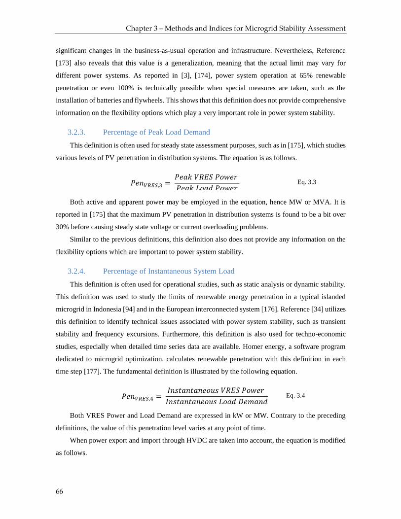
Chapter 3 – Methods and Indices for Microgrid Stability Assessment
66
significant changes in the business-as-usual operation and infrastructure. Nevertheless, Reference
[173] also reveals that this value is a generalization, meaning that the actual limit may vary for
different power systems. As reported in [3], [174], power system operation at 65% renewable
penetration or even 100% is technically possible when special measures are taken, such as the
installation of batteries and flywheels. This shows that this definition does not provide comprehensive
information on the flexibility options which play a very important role in power system stability.
3.2.3. Percentage of Peak Load Demand
This definition is often used for steady state assessment purposes, such as in [175], which studies
various levels of PV penetration in distribution systems. The equation is as follows.
𝑃𝑒𝑛𝑉𝑅𝐸𝑆,3 = 𝑃𝑒𝑎𝑘 𝑉𝑅𝐸𝑆 𝑃𝑜𝑤𝑒𝑟
𝑃𝑒𝑎𝑘 𝐿𝑜𝑎𝑑 𝑃𝑜𝑤𝑒𝑟 Eq. 3.3
Both active and apparent power may be employed in the equation, hence MW or MVA. It is
reported in [175] that the maximum PV penetration in distribution systems is found to be a bit over
30% before causing steady state voltage or current overloading problems.
Similar to the previous definitions, this definition also does not provide any information on the
flexibility options which are important to power system stability.
3.2.4. Percentage of Instantaneous System Load
This definition is often used for operational studies, such as static analysis or dynamic stability.
This definition was used to study the limits of renewable energy penetration in a typical islanded
microgrid in Indonesia [94] and in the European interconnected system [176]. Reference [34] utilizes
this definition to identify technical issues associated with power system stability, such as transient
stability and frequency excursions. Furthermore, this definition is also used for techno-economic
studies, especially when detailed time series data are available. Homer energy, a software program
dedicated to microgrid optimization, calculates renewable penetration with this definition in each
time step [177]. The fundamental definition is illustrated by the following equation.
𝑃𝑒𝑛𝑉𝑅𝐸𝑆,4 = 𝐼𝑛𝑠𝑡𝑎𝑛𝑡𝑎𝑛𝑒𝑜𝑢𝑠 𝑉𝑅𝐸𝑆 𝑃𝑜𝑤𝑒𝑟
𝐼𝑛𝑠𝑡𝑎𝑛𝑡𝑎𝑛𝑒𝑜𝑢𝑠 𝐿𝑜𝑎𝑑 𝐷𝑒𝑚𝑎𝑛𝑑 Eq. 3.4
Both VRES Power and Load Demand are expressed in kW or MW. Contrary to the preceding
definitions, the value of this penetration level varies at any point of time.
When power export and import through HVDC are taken into account, the equation is modified
as follows.
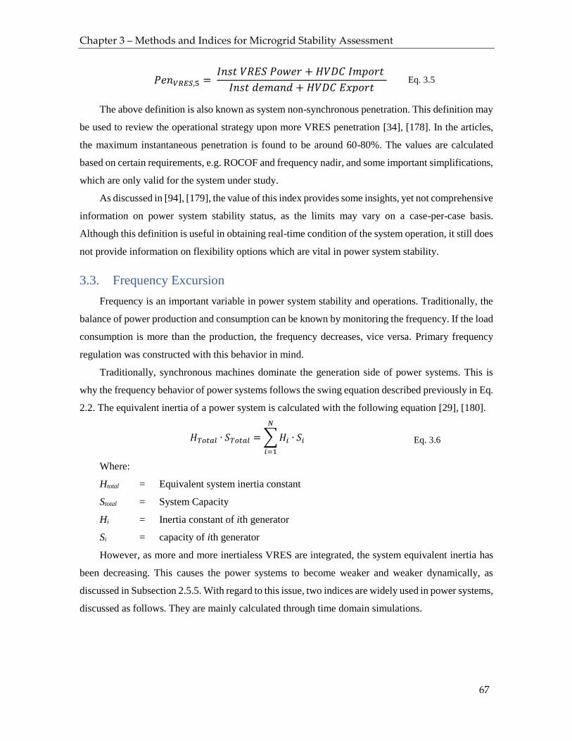
Chapter 3 – Methods and Indices for Microgrid Stability Assessment
67
𝑃𝑒𝑛𝑉𝑅𝐸𝑆,5 = 𝐼𝑛𝑠𝑡 𝑉𝑅𝐸𝑆 𝑃𝑜𝑤𝑒𝑟 + 𝐻𝑉𝐷𝐶 𝐼𝑚𝑝𝑜𝑟𝑡
𝐼𝑛𝑠𝑡 𝑑𝑒𝑚𝑎𝑛𝑑 + 𝐻𝑉𝐷𝐶 𝐸𝑥𝑝𝑜𝑟𝑡 Eq. 3.5
The above definition is also known as system non-synchronous penetration. This definition may
be used to review the operational strategy upon more VRES penetration [34], [178]. In the articles,
the maximum instantaneous penetration is found to be around 60-80%. The values are calculated
based on certain requirements, e.g. ROCOF and frequency nadir, and some important simplifications,
which are only valid for the system under study.
As discussed in [94], [179], the value of this index provides some insights, yet not comprehensive
information on power system stability status, as the limits may vary on a case-per-case basis.
Although this definition is useful in obtaining real-time condition of the system operation, it still does
not provide information on flexibility options which are vital in power system stability.
3.3. Frequency Excursion
Frequency is an important variable in power system stability and operations. Traditionally, the
balance of power production and consumption can be known by monitoring the frequency. If the load
consumption is more than the production, the frequency decreases, vice versa. Primary frequency
regulation was constructed with this behavior in mind.
Traditionally, synchronous machines dominate the generation side of power systems. This is
why the frequency behavior of power systems follows the swing equation described previously in Eq.
2.2. The equivalent inertia of a power system is calculated with the following equation [29], [180].
𝐻𝑇𝑜𝑡𝑎𝑙 ∙ 𝑆𝑇𝑜𝑡𝑎𝑙 = ∑ 𝐻𝑖 ∙ 𝑆𝑖
𝑁
𝑖=1
Eq. 3.6
Where:
Htotal = Equivalent system inertia constant
Stotal = System Capacity
Hi = Inertia constant of ith generator
Si = capacity of ith generator
However, as more and more inertialess VRES are integrated, the system equivalent inertia has
been decreasing. This causes the power systems to become weaker and weaker dynamically, as
discussed in Subsection 2.5.5. With regard to this issue, two indices are widely used in power systems,
discussed as follows. They are mainly calculated through time domain simulations.

Chapter 3 – Methods and Indices for Microgrid Stability Assessment
68
3.3.1. Frequency Nadir
Frequency nadir is the lowest frequency recorded during a transient event, such as load impact
or loss of generator. The index is influenced by the magnitude of the transient event, the system
inertia, and the response of primary regulation. It is important as in many grid codes and norms, the
frequency limits are stated and grid operators have to satisfy the requirements. In addition, certain
protection schemes and load shedding actions are based on the frequency measurement.
Frequency nadir should not be confused with quasi steady state frequency. The latter relates to
the frequency after the response of primary regulation and before the activation of secondary
regulation, as illustrated in Figure 3.2.
Frequency nadir
Figure 3.2 – Illustration of Frequency Response Following a generation-demand imbalance
Frequency nadir is imposed in several grid codes and norms, through the operational frequency
limits, as shown in Table 2.7 and in [142]. Studies of maximum VRES level often use this index as
one of the limiting factors, such as the study of Irish power system [34] and Sulawesi power system
[181].
3.3.2. ROCOF
ROCOF is the time derivative of voltage frequency. In more detail, it corresponds to the
frequency gradient following an imbalance of active power generation and demand. It is defined
analytically as follows.
𝑅𝑂𝐶𝑂𝐹(𝑡) = 𝑑𝑓(𝑡)
𝑑𝑡 Eq. 3.7
With more and more renewables being integrated, the ROCOF is becoming higher. Two main
things are causing this: the lower system inertia and the higher and more frequent occurrence of power
imbalance due to the intermittency. Stable frequency is therefore more difficult to achieve.

Chapter 3 – Methods and Indices for Microgrid Stability Assessment
69
In reality, it can be measured by numerical approach, by measuring frequency at two points
separated by a defined time delay, also known as the measurement window. This is formulated by the
following equation.
𝑅𝑂𝐶𝑂𝐹(𝑡) = 𝑓(𝑡) − 𝑓(𝑡 − 𝑇)
𝑇 Eq. 3.8
Calculation methods and the choice of measurement window T are essential in the calculation,
as discussed in [88], [182]. Important dynamics may be missed when a large measurement window
is used, while the ripple and power quality problems may interfere with a small window [105]. IEEE
1547 requires that the ROCOF is calculated over an averaging window of at least 0.1 s [116]. Other
grid codes require 0.5s and 1s time windows, causing the measurement to be observable with time
delay [105].
In recent norms and grid codes, the ROCOF requirements for different generator technologies
started to appear. For instance, IEEE 1547 require DER to be able to ride through frequency
excursions having ROCOF up to 3 Hz/s [116], while some grid codes, such as Australian grid codes,
require wind farm to ride through for ROCOF as high as 4 Hz/s [142], [182].
Apart from the protection systems, ROCOF measurement is also be used in the regulation of
power electronics, such as in synthetic inertia response. ROCOF is also important in phase tracking
of power electronic apparatus. This will be discussed further in Subsection 4.3.
3.4. Indices based on PV and QV Curves
PV and QV curves are useful for voltage stability analysis. They visualize how close a certain
operating point to voltage instability. Distance to instability can be expressed through physical
quantities, such as load level or active/reactive power flow. A simple mathematical formulation can
be derived for a simple system consisting of a voltage source, transmission lines modeled as
impedance, and a load modeled as an impedance [29], which results in a typical curve illustrated in
Figure 3.3 (a). However, for a complex power system, the curve is constructed based on the load flow
analysis, such as used in [29], [94]. Consequently, only stable operating points up to its nose point
can be found, as power flow tends not to converge beyond this limit. This is illustrated in Figure 3.3
(b).

Chapter 3 – Methods and Indices for Microgrid Stability Assessment
70
0 0.2 0.4 0.6 0.8 1 1.2P/Pmax
0
0.1
0.2
0.3
0.4
0.5
0.6
0.7
0.8
0.9
1
Vr
(a)
0.00
1.00
0.80
0.60
0.40
0.20
0.00
1.601.200.800.40
P (MW)
Vr
[p.u
.]
Nose point
2.00
(b)
Nose point
Figure 3.3 – Typical PV Curves at constant Power Factor
The active or reactive power shown in PV or QV curves may correspond to the power at a certain
bus or feeder. In the former, the Vr is taken at the associated bus while the latter, at the feeder end.
Since the analysis is based on load flow analysis, sensitivity analysis to active and reactive power
can be carried out. Voltage instability, occurring at the nose point, is closer when dV/dP or dV/dQ
increases, and occurs when dV/dP or dV/dQ is very high [29]. PV and QV curve-based analyses are
also applicable for microgrids in the presence of significant IBG [122].
Various voltage stability indices are reviewed in [183], most of which serve as a proximity
indicator to voltage instability and are derived from PV or QV curves. The values of the indices
typically range from 0 to 1. Voltage instability occurs at either one of two extremities. Another useful
index relating to loadability can be obtained by calculating the ratio of the critical loading, which
causes voltage instability, to the current loading. The loadability index indicates how far the bus under
consideration can be loaded with respect to the current loading.
Several voltage stability indices are listed in Table 3.2.
Table 3.2 – Some Voltage Stability Indices
Index Equation Note
Voltage Stability Index (VSI) [184]
𝑉𝑆𝐼𝑖 = 1 + (𝐼𝑖
𝑉𝑖) (
∆𝑉𝑖
∆𝐼𝑖) Eq. 3.9
Instability at VSI = 0
∆ = incremental change
I = load current
Loadability index 𝐿𝑖 = 𝑃𝑖,𝑐𝑟𝑖𝑡
𝑃𝑖,𝑜𝑝 Eq. 3.10
Should be accompanied by power
factor
op = operating point, crit = critical
3.5. Proposed New Indices
When dealing with power system stability, the balance of power production and consumption
must be maintained. However, doing it at all times upon every possible scenario is impractical and

Chapter 3 – Methods and Indices for Microgrid Stability Assessment
71
uneconomical. The best practice is only to anticipate credible scenarios. In order to do this, a list of
credible scenarios must be firstly defined.
Traditionally, power systems are designed to comply with N-1 criterion. This means that a power
system is planned such that, with all facilities are in service, it is operating in a secure state, and with
one credible contingency event, the system moves to a satisfactory state. ENTSO-E requires that the
frequency containment reserves, defined as the operational reserves activated to contain system
frequency after the occurrence of an imbalance, is sized to the reference incident that may cause the
biggest active power imbalance with an N-1 failure [40]. The same is also widely practiced in the
industry. However, due to the intermittent nature of variable renewables in power systems, it becomes
more complicated to define and satisfy the N-1 criterion. The novel indices still stick with the
necessary condition of maintaining power equilibrium upon credible scenarios since failure to do so
may result in undesired blackouts. This approach is therefore deterministic. However, the way that
the scenarios are considered evolves as both generation and demand may be either variable or
controllable. The factors to take into account may vary based on the type of the microgrid and the
flexibility available for use.
The factors that must be taken into consideration in power system stability are shown in Table
3.3. Here, we are trying to be as general as possible in terms of microgrids considered.
Table 3.3 – Factors Influencing Power System Stability
No Factor Explanation
1 Credible
Disturbance Loss of largest plant (N-1 criterion), Predictability of
Loads and VRES
2 Nature of Credible
Disturbance Step or ramp, time response
3 Flexibility Options
Fast response generators, governor tuning, storage, VRES curtailment,
demand side management (communication and non-communication based), interconnection
In the above table, VRES curtailment is a condition where the production from VRES is
intentionally curtailed from its maximum potential. The objective may be twofold: to avoid
overproduction of active power and to help maintain grid stability. For the latter, it serves similarly
to primary reserve. Demand side management consists of two methods: communication-based and
non-communication based. In the former, a central supervision system sends out orders to non-critical
loads to respond to system conditions. In the latter, decentralized controls which respond to frequency
and voltage excursions may be used. In this regard, it is similar to load shedding. Additionally, some
grid codes authorize brownouts, an action in which the grid voltage is intentionally decreased to
reduce the power demand [94], [103], [185].

Chapter 3 – Methods and Indices for Microgrid Stability Assessment
72
Dynamic balancing problem is illustrated in Figure 3.4. In this analogy, the deviation of the scale
from the horizontal axis is analogous to the frequency deviation from the nominal value. The shaded
boxes are subject to variability. In physics, the response speed of the scale due to weight imbalance
depends on the gravitational acceleration. In this illustration, the gravitational acceleration is
inversely proportional to the system inertia, meaning that the frequency deviates more when the
inertia is low. The flexibility options are chosen based on the priority set by the system operator. The
controls and activation strategy of the flexibility can be local or centralized.
Interconnec-
tion
Storage
Dispatched
Generation
Dump Loads
VRES
GenerationCritical
Loads
Non-Critical
Loads
Dispatchable
Generation
Curtailed
VRES
g ~ 1/system inertia
Figure 3.4 – Illustration of Flexibility in Dynamic Balancing
In the literature, the maximum penetration level is often seen from grid code’s point of view. If
a loss of the largest power plant results in a frequency violation, the maximum VRES penetration has
been exceeded [34], [176], [186]. One major problem that arises from this approach relates to the
simplifying assumptions. For example, the event is the largest generation loss, which might not the
worst case scenario. The coincident production drop of VRES can be of higher magnitude. For
comparison, if an isolated microgrid is operating at 80% VRES from PV, cloud cover on solar panels
could drop that capability by as much as half in under 60 seconds [129]. Furthermore, sometimes it
is assumed that sufficient primary reserve can always be dispatched [176], which is not true. On top
of that, one should ask a question concerning the relation between frequency violation based on grid
codes and power system stability. A power system can return to a stable frequency upon an important
perturbation even though the frequency limit is violated temporarily in the process.
There is not a single critical instantaneous penetration rate since the system dynamics depend on
several factors that change from one period to the other [94], [176].
The indices associated to VRES penetration that we propose are presented as follows.

Chapter 3 – Methods and Indices for Microgrid Stability Assessment
73
Table 3.4 – Proposed Indices of VRES Penetration for Microgrid Stability Assessment
Index Equation
Des
ign
In
dic
es
VRES Mix Index 𝐼𝐷1 =�̂�𝑉𝑅𝐸𝑆
∑ 𝑃𝑑𝑖𝑠𝑝𝑎𝑡𝑐ℎ𝑎𝑏𝑙𝑒 + �̂�𝑉𝑅𝐸𝑆
Eq. 3.11
Generation-side readiness
index 𝐼𝐷2 =
∑ 𝑃𝑑𝑖𝑠𝑝𝑎𝑡𝑐ℎ𝑎𝑏𝑙𝑒 + ∑ 𝑃𝑠𝑡𝑜𝑟𝑎𝑔𝑒 − 𝑃𝑚𝑎𝑥 𝑢𝑛𝑖𝑡
�̂�𝑑𝑒𝑚𝑎𝑛𝑑
Eq. 3.12
Critical-load supply index
𝐼𝐷3 =�̂�𝑐𝑟𝑖𝑡𝑖𝑐𝑎𝑙 𝑑𝑒𝑚𝑎𝑛𝑑
�̂�𝑑𝑒𝑚𝑎𝑛𝑑
Eq. 3.13
Mo
nit
ori
ng
ind
ex
Dynamic Stability Index
𝐼𝑀1 =𝑃𝑎𝑐𝑡𝑙 𝑔𝑒𝑛 + 𝑃𝑖𝑚𝑝𝑜𝑟𝑡 + 𝑃𝑃𝑟𝑖𝑚 − 𝑃𝑁−1
𝑃𝑐𝑟𝑖𝑡𝑖𝑐𝑎𝑙 𝑑𝑒𝑚𝑎𝑛𝑑 Eq. 3.14
Where �̂�𝑉𝑅𝐸𝑆 is the anticipated maximum VRES production, 𝑃𝑑𝑖𝑠𝑝𝑎𝑡𝑐ℎ𝑎𝑏𝑙𝑒 is the capacity of
dispatchable generation, 𝑃𝑠𝑡𝑜𝑟𝑎𝑔𝑒 is the capacity of storage elements, 𝑃𝑚𝑎𝑥 𝑢𝑛𝑖𝑡 is the highest unit
capacity of dispatchable and storage elements, �̂�𝑑𝑒𝑚𝑎𝑛𝑑 is the anticipated peak demand comprising
of both critical and non-critical loads, �̂�𝑐𝑟𝑖𝑡𝑖𝑐𝑎𝑙 𝑑𝑒𝑚𝑎𝑛𝑑 is the anticipated peak demand of critical loads,
𝑃𝑎𝑐𝑡𝑙 𝑔𝑒𝑛 is the actual generated active power, 𝑃𝑖𝑚𝑝𝑜𝑟𝑡 is the actual power import at interconnection
points, PPrim is the total available primary reserve, 𝑃𝑁−1 is the power loss due to the worst
contingency event, and 𝑃𝑐𝑟𝑖𝑡𝑖𝑐𝑎𝑙 𝑑𝑒𝑚𝑎𝑛𝑑 is the total actual demand of critical loads.
Design indices do not vary over time whereas the monitoring index does. Consequently, the
monitoring index needs to be constantly monitored. It should be noted that non-critical demand is
deemed to be available to participate in demand response but considered separately from the primary
reserve (𝑃𝑃𝑟𝑖𝑚) in the Table above. Only dispatchable generation and storage systems account for
PPrim. Regarding the total available primary reserve (𝑃𝑁−1), the capacity is taken into account for
dispatchable units and the total of actual generation plus curtailed power for VRES. Furthermore, the
interconnection is not taken into account in the design indices, reflecting the worst case off-grid mode
of operation. Here, the philosophy is to supply critical loads at any given time, while non-critical
loads are only supplied when the generation is available. For dynamic stability index, the contingency
under consideration may either be interconnection loss, VRES production drop, or largest generator
loss. It depends on the operation mode and the point of operation of the microgrid.
The VRES mix index differs from renewable penetration level PenVRES,2 in a way that instead of
the total capacity, it uses the total expected peak power production of installed VRES in the
calculation. This is due to the fact that some VRES generate electricity only during certain period of
the day. PVs only generate electricity during the daytime whereas in some regions, wind farm

Chapter 3 – Methods and Indices for Microgrid Stability Assessment
74
produces more electricity in the nighttime. Consequently, the peak VRES production may not be
identical to the total installed VRES capacity. With regard to supply and balance stability, the worst
case scenario relates to the sudden drop of VRES production at peak production. Therefore, taking
into account the peak VRES production is more representative stability-wise.
An illustration of the variables of design indices is introduced in Figure 3.5.
Peak
VRESDispatchable
GenerationStorage
Peak
Critical
Demand
Non-Critical
Demand
Dump
Load
production
demand
Peak demand
Maximum
unit
capacity
Figure 3.5 – Illustration of Variables Used in Design Indices
The indices can be thought of as a filter for microgrid practitioners. However, supplementary
power system stability studies may still be necessary to ensure the dynamic stability in different
configurations of microgrids. The assessment is typically performed through time domain
simulations, taking credible scenarios into consideration. It should be noted that a more thorough
analysis should also be conducted for off-peak periods because fewer synchronous generations are
online, resulting in lower system inertia.
The summary of indices useful for microgrid planning and operations in terms of stability issues
is as follows.
Table 3.5 – Indices and their Criteria
No Conditions Requirement(s)
1 Potentially stable, demand response not necessary
ID2≥1
2 Potentially stable, demand response necessary
ID2<1,ID2/ID3 ≥1
3 Potentially stable operation IM1 ≥1
4 High VRES penetration ID1≥predefined percentange
These indices reflect minimum necessary requirements, which signify that it is impossible to
guarantee power system stability without satisfying the indices. It should be noted that inertia
problems are not taken into account in the preliminary analysis.
The usability and the practicality of the indices have been tested against time-domain-simulation
data with satisfactory results, as reported in [165].

Chapter 3 – Methods and Indices for Microgrid Stability Assessment
75
3.6. Conclusion
A number of indices around power system stability in the presence of VRES have been discussed
in this chapter. Due to the advent of more inverter-based generators and the VRES, some indices need
to be rethought. For example, ride through capability should be added to critical clearing time
calculations. Some classical indices such as frequency excursions and voltage stability indices are
still useful in the IBG era, as most of the current inverter technologies are of grid feeding or grid
supporting types, which means they still rely on a grid former, such as synchronous generators, to
provide them with the voltage and frequency reference.
The definitions of the VRES penetration level are also reviewed to obtain better understanding
of their significance. Some indices provide technical meaning, while the others serve different
purposes, such as economic and political ones. From here, we conclude that the maximum VRES
penetration level varies on a case-by-case basis. We then propose a set of indices based on the power
equilibrium criteria, which are useful as a time-efficient filter to assess microgrid stability.

PART II
Efforts to preserve power system dynamic stability in
microgrids characterized by massive levels of
renewables

77
Chapter 4 Efforts to Accommodate Massive
Shares of VRES in Future Power Grids
In this chapter, the main challenges with regard to the power system stability due to more VRES
interconnection and the current efforts are reviewed, which have shown that the current solutions
focus on maintaining the philosophy of a classical power grid. With the advent of more and more
VRES, the current efforts have proven to be costly. Thus, a new perspective is proposed. Here, the
generating elements and the customers are exposed with higher deviations in main variables such as
the voltage and the frequency, which are necessary to maintain the power equilibrium and the stability
of the microgrid.
4.1. Introduction
Power systems are traditionally designed to comply with N-k (typically N-1) criterion in the
normal state [187]. This means that a power system is planned such that, with all facilities are in
service, it is operating in a secure state, and with one credible contingency event, the system moves
to a satisfactory state.
Following a contingency, the power system may enter alert state, where all the constraints are
satisfied but N-1 criterion is not assured anymore for certain contingency events. If the situation
aggravates, the system may move to emergency states, where some constraints are not satisfied
anymore. However, corrective actions such as generation tripping or load curtailment may still be
carried out and widespread blackout does not take place. If the perturbation is severe and the
corrective actions are not sufficient, the system may enter in extremis state. It is the condition where
cascaded blackouts occur, resulting in a shut-down of a major portion of the power system. Following
this, restorative actions where all the facilities, including generation, transmission, and loads, are
reconnected are carried out to restore the functionality of the power system. These states are illustrated
in Figure 4.1.

Chapter 4 Efforts to Accommodate Massive Shares of VRES in Future Power Grids
78
Figure 4.1 – Power System Operating States according to Kundur [29]
With more and more shares of variable renewables in power systems, it becomes more
complicated to satisfy the N-1 criterion at all times, notably concerning the problem of maintaining
the power balance between production and consumption. Classically, generators are operated such
that upon any trip of a single unit of generator, the system moves to a new satisfactory state without
any load shedding. Thus, it is necessary to have total grid spinning reserve of at least the active power
rating of the largest unit of generator in service. In the worst case scenario and with insufficient
spinning reserve, an event (e.g. largest generator loss) may cause continuingly decreasing frequency
and eventually may result in a blackout.
Not satisfying N-k (typically N-1) criterion creates higher risk of blackouts, as pointed out in
[188]. The Initiating events vary from case to case, ranging from protection failures or
malfunctioning, overloading, faults, natural disasters, to terrorist attacks [188]–[191]. The initiating
event may then be followed by cascading events leading to widespread loss of elements, known as
blackouts. Major blackouts typically occur as a result of the inability of the power system to support
the demand for generation power delivery [192].
4.2. Main Challenges
The grid of the future is discussed previously in Subsection 2.4.2. Renewable energy is one of
the key axes of the grid of the future. More and more intermittent renewables are interconnected to
power systems nowadays through inverter interface. This initially created only few problems when
the proportion was still low. However, as more and more VRES are integrated into power systems
through inverters, some issues started to arise, notably lack of inertia and energy intermittency. These
two factors have a great impact on power system stability, especially on frequency stability.

Chapter 4 Efforts to Accommodate Massive Shares of VRES in Future Power Grids
79
The topic of achieving 100% renewable grid is discussed in [193]. Several countries have
successfully operated their grids with high levels of renewables based on hydropower and geothermal,
such as Norway, Iceland, and Costa Rica (above 90% based on annual energy generated). However,
systems like these are limited by geographic topology and natural resources. Around the world, other
areas have the possibility to achieve 100% renewable grids by exploiting variable renewable energy
options, such as wind and PV systems. With the reduction in costs during the last decade, large-scale
deployments are a taking place around the globe.
4.2.1. Variability and Predictability
VRES are different from thermal generators because of the variability and uncertainty of the
outputs. Grid-wise, the challenges of grid operations become more apparent as the imbalance between
power production and consumption occurs more frequently in higher magnitudes. VRES are not
dispatchable and thus require greater grid flexibility in grid operations, as discussed in Subsection
2.4.3.
Figure 4.2 – types of power active power imbalance according to ENTSO-E [40]
In terms of imbalance phenomena in power systems, ENTSO-E classifies them into four types,
as depicted in Figure 4.2. Traditionally, type 1 is the worst case. However, with more and more
intermittent sources, type 3 can be problematic for the grid operator. In PV installations, the irradiance
may drop 75% in less than 40 seconds, such as the case in Indonesia [186], which increases the
complication of operating a microgrid at high levels of VRES.
Reserve margin is a function of the load factor, the load factor, the magnitude of the load, the
load shape, reliability requirements, and the availability of the DER [112]. In island mode, there is a

Chapter 4 Efforts to Accommodate Massive Shares of VRES in Future Power Grids
80
need to provide dynamic response from the DER. For example, following a motor starting, the DER
should be able to maintain voltage and frequency stability. Transient stability following perturbations
such as load steps, DER unit outage, and faults, should be maintained. There should be enough
monitoring to operate and understand the status of the island. If multiple DER units exist in the island,
their operation should be managed and coordinated to meet the needs of the island.
In rural areas, the lack of skills of locals in grid management makes it even more difficult to
forecast the stochastic behavior of loads and VRES. Consequently, blackouts occur frequently with
today’s grid regulation and management.
4.2.2. Low inertia
The other major phenomenon is the lack of inertia. With the present strategy of grid regulation,
this issue contributes to more frequent and significant frequency deviation. Traditionally, the grids
are dominated by conventional synchronous generators. As opposed to inverters, they have stationary
part (stator) and rotating part (rotor) which produce a rotating magnetic field, which induces a voltage
within the stator windings. This process creates AC electricity at a specified voltage and frequency
levels. These machines have important characteristics which have dictated how power systems have
been planned and operated since its first conception. This includes the swing equation, as well as
voltage and frequency regulations.
From a physics point of view, the turbine system and rotating components of synchronous
machines exhibit mechanical inertia, which stores kinetic energy in the rotating mass. That energy
can be extracted from or absorbed into these rotating masses in case of system perturbations, so that
the power systems can withstand temporary fluctuations in net load and generation. In contrast, VRE
technologies employ different technologies for energy conversion and interfacing to the grid. Aside
from concentrating solar power, VRES are typically integrated to the AC grid through inverters. The
associated controllers are executed on digital controllers where real-time measurements are processed
and processed. User defined controls are programmed and executed continuously. It is noteworthy
that the chosen control strategy, instead of inverter’s physical properties, dictates the electrical
dynamics of the inverters during disturbances and how they interact with the grid [193]. This poses
both challenge and opportunity to control engineers. Since no physical inertial response is available
on inverter’s power converting process, they are often said to have zero inertia. However, if
appropriate controls are applied, they can help improve the grid stability.
A literature study on the low inertia power systems are reported in [194]. In a hypothetical system
where there are no synchronous machines at all, the frequency is fully decoupled from the power
balance of the system, except if supplementary controls are in force. In this case, no element of the

Chapter 4 Efforts to Accommodate Massive Shares of VRES in Future Power Grids
81
grid responds naturally to power imbalance and a control system must be in place to preserve the
power balance at every instant. Here, the electrical frequency may still be a global variable, but is not
anymore a physical variable associated to the rotating magnetic field of synchronous machines.
Instead, it is a controlled variable.
Since IBGs do not naturally respond to power variations, specifically designed controls are
necessary. The inertial response can be implemented as a control loop, and is thus subject to delays,
malfunctioning, saturation, and other unexpected dynamics that may lead to instabilities. In addition,
some strategies are dependent on communication systems and are, in general, neither fully reliable
nor easy to implement.
In future very low inertia power systems, the roles of synchronous machines have to be replaced
by other grid formers, which will be discussed in Subsection 4.3.4. The current strategy of IBGs as
grid followers will no longer work because the reference of voltage and frequency is required.
Principally, the stability problems do not change much: voltage collapse, transient stability, and
frequency stability. Transient stability may not be as important as before as inverters are not
inherently regulated by the swing equation. Although the swing equation can be embedded into
inverter regulation strategy, the out of synchronism phenomenon can be avoided with supplementary
algorithms. However, problems caused by the grid configuration and transfer impedance such as
voltage collapse stay the same.
4.2.3. Additional Challenges for Microgrids
Currently, most islanded microgrids rely on fossil-based synchronous generators to provide
voltage and frequency reference [129]. In developing countries around the world, the main objectives
of small island systems and isolated networks are to provide universal energy access and to move
away from the dependency on fossil fuel transport [127]. Such areas typically lack skilled human
forces. Thus, simple operation and reliable devices are necessary so that minimum operation and
maintenance efforts are required. In addition, industrial activities which demand high quality
electricity are minimal in such areas, and residential loads dominate. Consequently, affordable
electricity is of high importance and high power quality is not top priority, as the point here is to
improve the living quality and the human development index.
Microgrids are different from large interconnected grids in many aspects. Microgrids do not have
to be compatible with the legacy-system [194]. As pointed out in [131], remote microgrids are
normally isolated and the power quality requirement is relaxed. Maximum power use may be limited
for the customers. It is difficult to maintain the standard level of voltage, frequency, and power quality
while preserving the balance between intermittent supply and fluctuating demand.

Chapter 4 Efforts to Accommodate Massive Shares of VRES in Future Power Grids
82
4.3. Current Efforts
Efforts are needed to tackle the challenges of the grid of the future. Researchers and engineers
propose numerous strategies and approaches to deal with the challenges of high levels of VRES. The
efforts to deal with variable renewables in the form of flexibility are reviewed previously in
Subsection 2.4.3. Here, the other aspects are discussed.
4.3.1. Efforts to improve predictability
Predictability is the key to better grid operation. Meteorological forecasting, while steadily
improving, is still subject to uncertainty. In this sense, the challenge with VRES is not so much its
variability, but rather its predictability. If output could be forecast with 100% certainty, the only
challenge would be to meet the ramp rates. Forecasting technologies are particularly important for
wave, wind, and solar technologies, the output of which varies irregularly. The tidal resource also
varies, but is well predictable. Flexibility in grids also fluctuates. It varies over time, and with the
extent of demand. VRES can be predicted with greater accuracy as the time ahead of delivery reduces,
reducing the need for the fast-response, high-premium variety.
Demand for electricity, being based on regularly repeating patterns of social behavior, may be
relatively easy to predict. However, unexpected peaks can still occur: as temperatures rise or fall
unexpectedly, or system wide consumer behavior coincides for other reasons. Experience has shown
that sometimes the forecast fits the reality, sometimes it does not. For example, generation of PV
plants in cloudy days is not very predictable [169]. Improving the predictability by refining the
forecasting method is the most straightforward way. Furthermore, there exist three important efforts
to improve the predictability of VRES: choosing anti-coincident sites – larger area interconnection,
balancing anti-coincident renewables, such as wind and solar, and employing dispatchable
renewables, such as hydro and geothermal [169].
4.3.2. Regulatory Efforts
The recent energy transition towards large-scale integration of renewables into power systems is
leading grid operators and standards bodies to specify more stringent operation and flexibility
requirements for generating equipment in order to assure the power system operation and stability.
For all technologies of DER, both classical synchronous machines or VRES connected through
inverters, new capabilities with regard to fault ride through, frequency range and control, ramp rates
requirement, reactive range and voltage control start to be required [99].
4.3.2.1. Fault Ride Through

Chapter 4 Efforts to Accommodate Massive Shares of VRES in Future Power Grids
83
Recent standards and grid codes mandate voltage and frequency ride through capabilities state
for all technologies of generating units in order to support the grid stability [48], [116], [142], [149].
IEEE 1547 defines ride through capability is defined as the ability to withstand voltage or frequency
disturbances inside defined limits and continue operating [116], while the EU Network code defines
it as the capability of a generator to be able to remain connected to the network and operate though
periods of low voltage at the connected point caused by secured faults [182], [195]. Some ride through
requirements imposed by a number of grid codes are illustrated in Figure 4.3 and Table 4.1. The
generator may disconnect outside the defined ride through requirements [116], [164].
Figure 4.3 – Comparison of Several Voltage Ride Trough Requirements [142]
Table 4.1 – Comparison of Several Frequency Ride Trough Requirements [142]
Frequency (Hz) Denmark French SEI Great Britain Ireland Spain SEIE
52-54 5 s 51.5-52 15 mn 1 h 51-51.5 15 mn 90 mn 60 mn 50.5-51 49.5-50.5 Cont. Cont. Cont. Cont. Cont. 49.49.5 5 h 48-49 30 mn 90 mn 60 mn 47.5-48 3 mn 1 h 47-47.5 20 s 3 mn 20 s 20 s 3 s 46-47 44-46 30 s
4.3.2.2. Wider range of operation
Operators have started to require DER to be capable of functioning in wider range of frequency
and voltage. In European grid, the protection settings for automatic disconnection of DER from the
grid are formerly not in line with those of the transmission system. The settings for distributed
generation are in the range of 50.2 - 50.5 Hz for over frequency and around 49.8- 49.5 Hz for under
frequency whereas the ranges to mandatory remain connected within the European transmission
system is 47.5 - 51.5 Hz [196]. This results in some countries with a significant capacity of installed
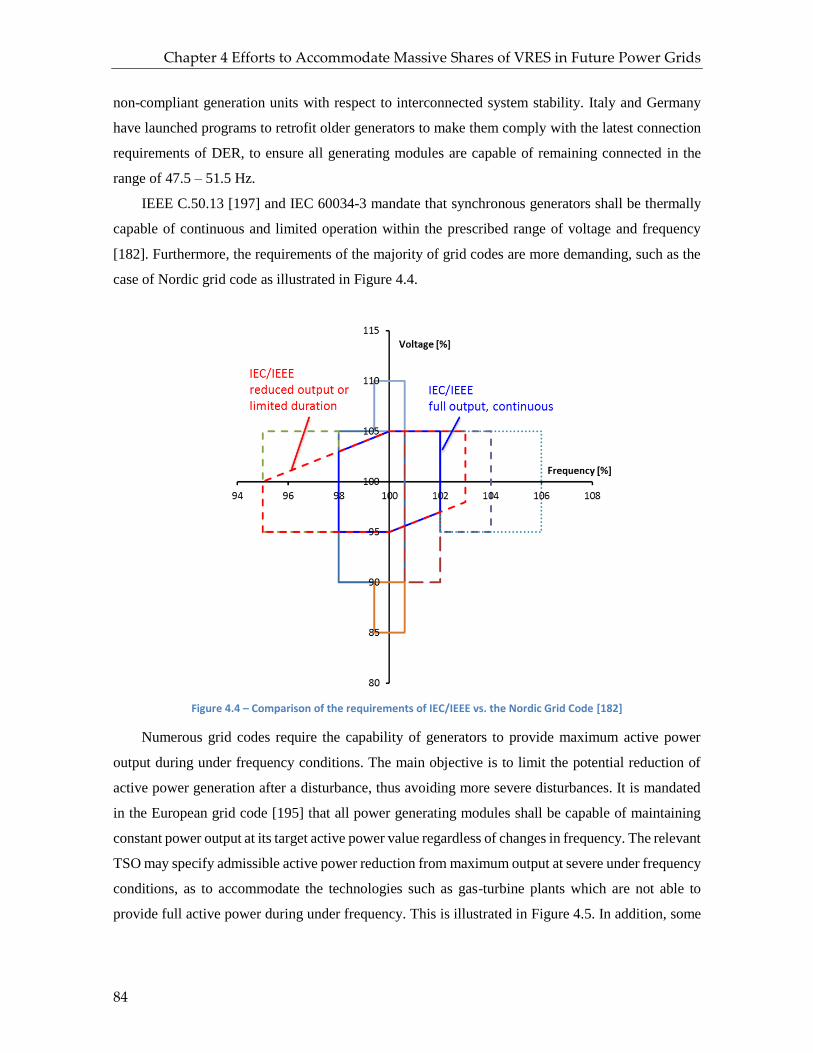
Chapter 4 Efforts to Accommodate Massive Shares of VRES in Future Power Grids
84
non-compliant generation units with respect to interconnected system stability. Italy and Germany
have launched programs to retrofit older generators to make them comply with the latest connection
requirements of DER, to ensure all generating modules are capable of remaining connected in the
range of 47.5 – 51.5 Hz.
IEEE C.50.13 [197] and IEC 60034-3 mandate that synchronous generators shall be thermally
capable of continuous and limited operation within the prescribed range of voltage and frequency
[182]. Furthermore, the requirements of the majority of grid codes are more demanding, such as the
case of Nordic grid code as illustrated in Figure 4.4.
Figure 4.4 – Comparison of the requirements of IEC/IEEE vs. the Nordic Grid Code [182]
Numerous grid codes require the capability of generators to provide maximum active power
output during under frequency conditions. The main objective is to limit the potential reduction of
active power generation after a disturbance, thus avoiding more severe disturbances. It is mandated
in the European grid code [195] that all power generating modules shall be capable of maintaining
constant power output at its target active power value regardless of changes in frequency. The relevant
TSO may specify admissible active power reduction from maximum output at severe under frequency
conditions, as to accommodate the technologies such as gas-turbine plants which are not able to
provide full active power during under frequency. This is illustrated in Figure 4.5. In addition, some
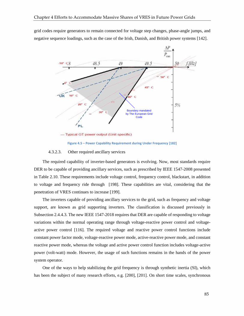
Chapter 4 Efforts to Accommodate Massive Shares of VRES in Future Power Grids
85
grid codes require generators to remain connected for voltage step changes, phase-angle jumps, and
negative sequence loadings, such as the case of the Irish, Danish, and British power systems [142].
Boundary mandated
by The European Grid
Code
Figure 4.5 – Power Capability Requirement during Under Frequency [182]
4.3.2.3. Other required ancillary services
The required capability of inverter-based generators is evolving. Now, most standards require
DER to be capable of providing ancillary services, such as prescribed by IEEE 1547-2008 presented
in Table 2.10. These requirements include voltage control, frequency control, blackstart, in addition
to voltage and frequency ride through [198]. These capabilities are vital, considering that the
penetration of VRES continues to increase [199].
The inverters capable of providing ancillary services to the grid, such as frequency and voltage
support, are known as grid supporting inverters. The classification is discussed previously in
Subsection 2.4.4.3. The new IEEE 1547-2018 requires that DER are capable of responding to voltage
variations within the normal operating range through voltage-reactive power control and voltage-
active power control [116]. The required voltage and reactive power control functions include
constant power factor mode, voltage-reactive power mode, active-reactive power mode, and constant
reactive power mode, whereas the voltage and active power control function includes voltage-active
power (volt-watt) mode. However, the usage of such functions remains in the hands of the power
system operator.
One of the ways to help stabilizing the grid frequency is through synthetic inertia (SI), which
has been the subject of many research efforts, e.g. [200], [201]. On short time scales, synchronous

Chapter 4 Efforts to Accommodate Massive Shares of VRES in Future Power Grids
86
machines maintain the power balance through instantaneously available physical storage in the form
of inertia, and later through their primary control which takes effect more slowly. In contrast, IBG
works differently: the analogy of synchronous machine’s inertia is the energy stored in the DC-side
capacitor, which is typically much smaller compared to the synchronous machine’s inertia of the same
power capacity. On the other hand, power electronic sources can be actuated on much faster time
scales and thus contribute to power balancing, provided that the DC-side energy supply is capable of
supporting this. Consequently, the lack of physical inertia can potentially be compensated through
fast DC-side energy storage equipped with appropriate control strategies.
In contrast to synchronous machines, frequency changes have to be detected first by the control
systems. Applied filtering might lead to time delays and thus reduce the performance of emulated
inertial response [34]. If the delays are too long, then the synthetic inertia (SI) will provide no
mitigation of the initial ROCOF during an event. If the delay happens to lead to a phase lag that is
180 degrees different to the equivalent true inertial response, then the output power modulation
provided by the SI can operate in complete anti-phase to the rotor swings of a real synchronous
machine, encouraging classical rotor oscillations, and thereby degrading network stability [105].
4.3.3. Operational Efforts
With regard to intermittent renewables, John Reilly from NREL proposes the following actions
to deal with the VRES and to assure power supply [169]: balancing with storage, such as pumped
hydro or battery, and balancing with dispatchable generation plants, such as natural gas turbine or
combined cycle plants.
In very high level of VRES scenarios (60-100% energy-based), batteries and demand response
are deemed important in order to maintain the balance of active power production and consumption,
as reported in [129], [202]. Primary reserve with droop-like response may also be carried out by
VRES via active power curtailment [55]. However, this strategy results in curtailed energy, as the
harvested energy is curtailed form the maximum potential, which is normally not desired.
Demand response can be accomplished with the support of communication or local
measurements. ICT, previously discussed in Subsection 2.4.4.1, plays an important role in this
function. Load shedding is still considered important as the last resort to maintaining frequency
stability. The details of operational efforts are also reviewed in Section 3.5, and the significance of
the efforts can be assessed through the proposed indices [165].
4.3.4. Technical Efforts
With regard to technical issues introduced by the variability and low inertia, the French
transmission system operator, RTE, identified 2 possible solutions: synchronous condensers and grid

Chapter 4 Efforts to Accommodate Massive Shares of VRES in Future Power Grids
87
forming inverter technologies, e.g. virtual synchronous machine [203], both of which are able to fill
in the role of (dispatchable) synchronous generators, notably with regard to the capability to provide
voltage and frequency reference and to stabilize the grid upon perturbations.
4.3.4.1. Synchronous condensers
Synchronous condensers are synchronous machines which are not connected to any mechanical
loads or turbines, hence not dispatchable. They were formerly used mostly only for reactive power
source. However, as the penetration of IBG increases, other key features of synchronous condensers
which may help stabilize the grid are sought after, such as high short circuit current and voltage
recovery capability, inertial response, and the capability to provide the reference of voltage and
frequency.
This technology has long been identified as a solution for power infeed through line-commutated
HVDC to a weak system, or even to a system without any generation, due to its capability to maintain
frequency and voltage at an acceptable levels during system perturbations and its inherent inertia
[204]. However, until recently, there was not much interest into this technology because power
systems were supplied mostly by dispatchable synchronous machines, hence enough inertia.
However, as the penetration of VRES keeps increasing, several engineering companies and TSOs
started to show interest in this relatively mature technology, such as ABB [205] and Siemens [206].
Siemens even states that the synchronous condensers are a proven solution to stabilize the grid.
Projects of conversion of old synchronous generators to synchronous condensers have marked the
revival of synchronous condensers, such as the conversion of Biblis nuclear power plant in Germany
in 2012 and Ensted coal-fired power plant in Denmark in 2013 [207].
AC
Grid
Voltage
regulator
Excitation voltage
Grid voltage
Synchronous
condenser
Figure 4.6 – Synchronous condenser structure

Chapter 4 Efforts to Accommodate Massive Shares of VRES in Future Power Grids
88
A project called Synchronous condensers application in low inertia systems, under the
collaboration of the Technical University of Denmark and Siemens, was launched in 2015 as an effort
to find a solution to problems introduced by high levels of IBG interconnection [208]–[211].
As the majority of IBG are of grid following and grid supporting type, synchronous condenser
technology could be a straightforward solution to the grid stability problem, where the VRES
connected via IBG are responsible for power generation and the synchronous machine for grid
stability and the reference of voltage and frequency. This concept and the construction of the machine
are well understood by researchers and engineers, as the technology is already mature. The classical
inherent behavior of synchronous machines and power systems based on the swing equation is still
applicable here, hence familiarity with the classical power system engineering practice. An important
downside of active power losses has to be taken into account in the operation.
In this PhD thesis, we propose new power system regulation strategy suitable with this
technology, which will be thoroughly discussed in Chapter 5.
4.3.4.2. Grid forming inverters
A grid forming inverter is an inverter which has the capability to form a grid, i.e. to provide
voltage and frequency reference to the grid. This approach typically requires controllable and fast
response energy storage on the DC side. A grid forming inverter can be modeled as a voltage source
parallel with low impedance, as discussed in Subsection 2.4.4.3. It should be capable of providing a
reference and support for frequency and voltage, robust synchronization mechanism, and performing
black-start, all of which are traditionally offered primarily by synchronous machines [194].
Inverters have no natural interactions with the AC grid. The interactions between the IBG, the
other resources, and the grid are therefore determined by the chosen control approach. An important
limitation of inverters that has to be taken into consideration is the narrow limits of current overshoots,
as opposed to high overloading and overcurrent capability of synchronous machines.
Virtual synchronous machine (VSM) is one of the control strategies of grid forming inverters.
The concept was introduced in 2008 by Driesen and Visscher [212]. The idea is to help stabilize the
grid by controlling an inverter (or a group of inverters) to emulate the characteristics of a synchronous
machine, including the inertia, damping properties, and primary regulations (i.e. frequency and
voltage droop). Existing VSG topologies and applications are reviewed in [213]–[215] while a review
of detailed control strategies of VSM is presented in [216]. Contrary to synchronous machines which
have inherent synchronization mechanism, the VSM need a synchronization unit. Currently, some
strategies use a PLL to provide the phase and frequency of the grid voltage as to attain smooth
synchronization. However, PLLs may cause many problems leading to reduced performance,

Chapter 4 Efforts to Accommodate Massive Shares of VRES in Future Power Grids
89
increased complexity, or even instability [215]. Recent advances have shown that a VSM can
synchronize itself with the grid an embedded synchronization mechanism and therefore the PLL can
be removed. This concept is called self-synchronized synchronverter [217]. Aside from higher
frequency noise due to static switching, there is no difference between the electrical appearance of an
electromechanical synchronous generator and a completely electrical virtual synchronous generator
within the unsaturated operating region from the grid point of view. As the inverters behave similarly
to synchronous machines, legacy practices in power systems are not much altered.
Some researchers commented that controlling a converter to behave like a synchronous machine
is wasteful as the key resources and strengths of the converter are not fully exploited, such as in [194].
However, as the power system world is accustomed to the notion introduced by synchronous
machines and its effectivity has been well proven, one can benefit from the understanding of how
power systems work with synchronous machine-like behavior and from the capability of virtual
synchronous machine to have dynamic parameters based on what is best for the power system.
inverter
AC
Grid
DC-side
Battery
Filter
VSM Control
Alorithm
VSM
Figure 4.7 – General structure of virtual synchronous machine
Other control strategies of grid forming inverters include stiff grid forming inverters widely
utilized in uninterruptible power supply (UPS). Stiff grid forming strategy behaves similarly to
perfect voltage source, which ensures that the terminal voltage and frequency are maintained at
nominal values at any moment. Consequently, load sharing and synchronization could be among
major problems when multiple grid formers function in the grid, particularly with the absence of a
global controller and fast communication systems.

Chapter 4 Efforts to Accommodate Massive Shares of VRES in Future Power Grids
90
4.4. New Perspective on Quality of Supply
The needs that a power system must serve will evolve over time, as discussed recently in early
2019 in IEEE power & energy magazine [218]. For most of the 20th century, the society needs
industrial growth, universal access to electricity, growth of cities and suburban areas, and expansion
of the customer economy. The 20th century power systems were constructed to serve a reliability
philosophy, where customers’ appliances must always come on when they switch them on. This drove
infrastructure investment to satisfy peak load conditions which occur only during short period. Now
in the 21st century, the societal needs of power systems have changed: reduction of greenhouses gases,
greater resilience to disruptive events, elimination of the bad health impacts due to fossil plants,
fostering a diverse and competitive arena of new energy technologies, and more options and control
of their energy sources and uses.
4.4.1. Driving force of Renewables
The main driving force behind renewable energy development is different in different places
across the globe. In Europe, it is to fight against green-house effects caused by fossil fuels. Due to
slow growth in electricity demand, old fossil-based generation plants have been envisaged to be
replaced by renewables. Whereas in developing countries where the electricity growth is tremendous
and some people still live without electricity, the motivation is to provide affordable universal
electricity and to respond to demand growth, meaning that the renewable plants are constructed with
the hope of increasing the system capacity.
Microgrids are important for economic development, as argued by the CEO of Homer [130].
However, all over the world, islanded microgrids often utilize diesel generators, which are noisy, not
eco-friendly, and expensive. As the price of renewable technologies such as PV and battery is
decreasing, the outlook seems to be in favor of VRES. This is a different segment of market with
separate value prepositions. In both grid connected and off-grid operating modes, a microgrid should
be capable of maintaining balance between power generation and consumption [68]. Government
agencies, utilities, military bases, universities, and research centers have been deploying microgrids,
and the positive trend is expected to continue in the next decade [132], driven by environmental
issues, the need for electricity in remote communities, and the prospect of increased resilience and
reliability. However, the focus objective may vary for different microgrids, as discussed in 2.5.1.
Reference [174] revealed that high penetration level of variable renewables often takes place in small
power systems (i.e. smaller than 100 MW), which fall into isolated microgrid category.

Chapter 4 Efforts to Accommodate Massive Shares of VRES in Future Power Grids
91
4.4.2. Views on Electric Power Quality and Grid Operation
In power grid operation, power quality nowadays is expected to be within certain strict
boundaries even at high levels of renewable penetration. Consequently, high investment and
operation costs are inevitable. The generation side is currently evolving with the integration of more
variable renewables. However, system regulation strategy does not change too much. Thus, power
systems are more prone to blackout due to the failure in maintaining the power balance. In many grid
operation schemes, load shedding serves as the last resort in order to avoid the in extremis state as
shown in Figure 4.1. It is triggered only when the imbalance is severe and it is typically
predetermined. Furthermore, the shed load might be more than necessary, which results in
overfrequency [219]. Reestablishing the frequency back to nominal values is normally carried out
later, which takes time. Only then will the shed load be brought back into service.
In order to reach 100% VRES, the grid may need to rely on the IBG for stability and grid
regulation, and thus standalone rules that are system dependent may be necessary [212]. In China, as
discussed in [3], there exists an operational microgrid composed by 7 MW of PV Units, 1 MW of
energy storage (2h of full discharge). When PV output decreases significantly, the security and
stability control will shed non-critical loads. The energy storage will be in discharging mode to
maintain the supply to critical loads. Then, other diesel generators will then be started and the shed
loads will be brought back into service. Obviously, this microgrid operation is different from how a
grid operation and regulation are normally managed.
Over the last decade, demand response has attracted much research attention. It is one of the
flexibility options in a power system. Its main idea is to shift the demand in order to suit the
availability of the supply. However, this strategy is typically realized with the support of (fast)
communication systems to send the price signals or dispatch instructions [220]–[222] or local
measurements which also require local computing resources (e.g. smart meters) [223]–[226].
The operational constraints in terms of voltage characteristics of electricity supplied by public
distribution systems required by EN 50160 [81] are illustrated in Figure 4.8. For various reasons, the
range is very strict for interconnected systems in steady state, while it is a bit less strict for islanded
grids. Momentary voltage and frequency deviations are allowed in wider ranges. As the inertia is
typically much lower in islanded grids, the permissible frequency deviations are relatively wider in
islanded systems.

Chapter 4 Efforts to Accommodate Massive Shares of VRES in Future Power Grids
92
10 20 30 40 50 60 70 80 90 100 110
10
20
30
40
50
60
70
80
90
100
110
0
Frequency [%]
Vo
lta
ge
[%
]
steady state, interconnected
Momentary, interconnected
steady state, islanded
Momentary, islanded
Figure 4.8 – Voltage characteristics of electricity supplied by public distribution systems required by EN 50160
As presented in Figure 4.8, even for momentary variations, the permissible limits are small
compared to the total area possibly covered, i.e. all areas where the frequency is lower than 84% are
not permitted, neither 0-50% of voltage. The strict operational ranges are imposed to guarantee the
power quality of electric supply in order to obtain satisfactory performance of electrical and electronic
appliances. Here, the focus is on the load side, to make sure that the loads are functioning properly
according to what is expected by the customers.
In terms of real units (in Volts and Hertz), the operational ranges for several appliances, notably
devices working with power supply, are wider even in steady state, as illustrated in Figure 4.9. The
values are based on a number of power supply design guides [227]–[230]. This indicates that certain
appliances in power systems are designed to function in wider range of voltage and frequency.

Chapter 4 Efforts to Accommodate Massive Shares of VRES in Future Power Grids
93
20 30 40 50 60
115
230
Frequency [Hz]
Vo
lta
ge
[V
]
Operation range
of power supply
265
90
47 63
Figure 4.9 – Ranges of operation of universal power supply [230]
As discussed previously in Subsection 4.4.1, the objective of the use of renewable energy and
the construction of microgrids varies across the globe. Consequently, the operation ranges should
adapt to the main objectives, especially in microgrids functioning with massive levels of renewables.
As suggested in [212], the operation and management of power systems with high penetration of
variable renewables may be different from the conventional ones. Several adjustments are necessary.
The grid codes may be unique only for a handful of cases. In this regard, if the main motive of a
microgrid development is for universal electricity access to low human development index (HDI)
regions, then the grid codes, as well as the management and operation, should be designed and
adjusted accordingly.
A key question arising here is why not utilize the degraded ranges (i.e. wider voltage and
frequency ranges) only momentarily for maintaining the power balance in the system and for reducing
the investment and operation costs. The approach indeed needs to take into account the impact on
the devices in the grid and the public acceptance.
4.4.3. Views on Energy Security, Reliability and Operating States
The topic of energy security is discussed in [231]. Although various definitions of energy
security exist in the literature, they all share a common idea that the energy supply should meet the
demand. In other words, abundant availability of energy sources is the key [232]. However, with the
integration of high levels of VRES, we encounter fundamental challenges to the current
understanding of energy security, notably due to their inherent intermittent behavior.

Chapter 4 Efforts to Accommodate Massive Shares of VRES in Future Power Grids
94
The US Department of Energy defines reliability as the ability of the system or its components
to withstand instability, uncontrolled events, cascading failures, or unanticipated loss of system
components. In the context of system planning, reliability-driven investment decisions are based on
N-k (typically N-1) reliability criterion [233].
IEEE PES Industry Technical Support Task Force defines resilience as the ability to withstand
and reduce the magnitude and/or duration of disruptive events, which includes the capability to
anticipate, absorb, adapt to, and/or rapidly recover from such an event [233]. The concept of resilience
covers all events, including high impact but unlikely events which are normally excluded from
reliability analysis. Both reliability, which is generally expressed by the number and duration of
power outages, and resilience, especially due to natural disasters, can be improved with microgrid
concept [234], as proven by the cases in Japan and the US.
Resilience-driven designs may not be aligned with reliability-driven ones. A study suggests that
for distribution systems, it is more resilience-effective to design a smarter and responsive network
than opting for more redundancy [235]. A widely used resilience diagram is shown as follows, which
goes along with the proposed operation states in microgrids marked with massive VRES in Figure
4.11.
Re
silie
nc
e L
ev
el
Time
Ro
to toe trtee T
Pre-disturbance resilient
stateDisturbance progress
Post-disturbance
degraded state Restorative state
Phase I Phase II Phase III
Rpd
Resilience Trapezoid
Post-restoration state
Figure 4.10 – Resilience Trapezoid associated with a disruptive event [233]
As far as islanded microgrids are concerned, maintaining high electrical energy security in the
presence of high levels of VRES is possible with the help of technologies such as storage systems,
but it is proven to be costly. A compromise between reliability, economic cost, and sustainability is
therefore necessary, with the focus on meeting the main objective of the grid. For example, if the
priority is to achieve optimum sustainable energy use at affordable cost, compromises in reliability
which requires customer behavior adjustment in electricity use are vital.
Here, we propose a new perspective which aligns with the demand response (DR) philosophy,
in regard to the view on maintaining the power balance in a power system using the demand side.

Chapter 4 Efforts to Accommodate Massive Shares of VRES in Future Power Grids
95
Instead of only ensuring that the generation side is capable of meeting the load demand; the loads
must follow the available power generation. In addition, the implementation should not depend on
predetermined load shedding, local measurements, or fast communication systems, which marks a
distinguishing point from a typical DR implementation. Consequently, this strategy is relatively
affordable and cost-effective. These features are highly desired in post-disaster recovery and low HDI
community cases. However, a tradeoff in power quality is inevitable. The technical implementation
of this proposal will be discussed in detail in Chapter 5.
With regard to energy security, the overall analysis should be comprehensive and consider other
types of energy besides electricity. The energy is principally needed for the daily activities, which
have certain flexibility in time. When measures such as variable frequency and voltage are taken, the
main question is whether or not that will still respond to the needs of the customers. In communities
previously living without electricity, the dependency and attachment to electricity are not yet
developed. Therefore, the introduction of electricity itself will increase the local energy security.
In the era where VRES dominate the generation side, the operation states as illustrated in Figure
4.1 becomes obsolete. The current definition of normal state and the requirement of N-1 criterion in
the generation side are not suitable anymore with massive VRES development, as the grid is rarely is
the “normal” operating state considering the worst expected contingency event (i.e. high variability
of VRES). The grid should now be considered secure in a sense that blackouts are evitable and the
system can reestablish normal operating conditions according to the (voluntary) actions of customers
and grid operator within the defined time following the perturbation. In addition, DR is not considered
the last resort anymore. It is one of the main flexibility to achieve power balance and power system
stability. However, load shedding of critical loads may be necessary when the degraded mode is still
ineffective. The proposed operation states in microgrids marked by massive penetration of VRES are
illustrated in Figure 4.11.
The illustrations of the grid operation and its proposed changes are shown in Figure 4.12 and
Figure 4.13. They depict the management of power equilibrium within the classical framework
(where generation should always meet the demand) and the new framework with massive VRES
characterized by DR.

Chapter 4 Efforts to Accommodate Massive Shares of VRES in Future Power Grids
96
Normal
Degraded
In Extremis
Restorative
Outside degraded
limits, blackout
System
reestablishment,
blackstart and
reconnection
No overloading,
voltage and
frequency within the
permissible normal
range, demand
response may be
carried out
Short term
overloading may
appear, voltage and
frequency within the
degraded range, load
shedding
N-1 criterion in
generation side is not
guaranteed anymore.
Positioned between
normal and alert
condition with respect
to the classical
operation states
Figure 4.11 – Operation States in Microgrids with Massive Levels of VRES
-3
-2
-1
0
1
2
3
4
5
0 0.5 1 1.5 2 2.5
Po
we
r (M
W)
Time (h)
Load
Renewables
Battery
-1
0
1
2
3
4
5
0 0.5 1 1.5 2 2.5
Po
we
r (M
W)
Time (h)
Load
Renewables
Curtailment/dumpload
Diesel
(a) (b)
Figure 4.12 – Classical Operation with N-1 criterion, normal operating state based on classical philosophy (a) Battery-VRES (e.g. PV) (b) Diesel-VRES-Curtailment
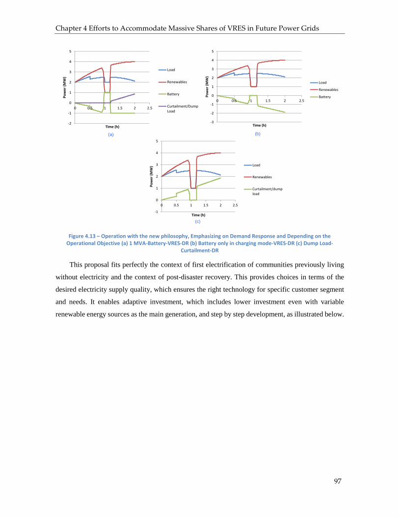
Chapter 4 Efforts to Accommodate Massive Shares of VRES in Future Power Grids
97
-3
-2
-1
0
1
2
3
4
5
0 0.5 1 1.5 2 2.5
Po
we
r (M
W)
Time (h)
Load
Renewables
Battery
-2
-1
0
1
2
3
4
5
0 0.5 1 1.5 2 2.5
Po
we
r (M
W)
Time (h)
Load
Renewables
Battery
Curtailment/DumpLoad
-1
0
1
2
3
4
5
0 0.5 1 1.5 2 2.5
Po
we
r (M
W)
Time (h)
Load
Renewables
Curtailment/dumpload
(a) (b)
(c)
Figure 4.13 – Operation with the new philosophy, Emphasizing on Demand Response and Depending on the Operational Objective (a) 1 MVA-Battery-VRES-DR (b) Battery only in charging mode-VRES-DR (c) Dump Load-
Curtailment-DR
This proposal fits perfectly the context of first electrification of communities previously living
without electricity and the context of post-disaster recovery. This provides choices in terms of the
desired electricity supply quality, which ensures the right technology for specific customer segment
and needs. It enables adaptive investment, which includes lower investment even with variable
renewable energy sources as the main generation, and step by step development, as illustrated below.

Chapter 4 Efforts to Accommodate Massive Shares of VRES in Future Power Grids
98
No electricity
Stimulus to HDI,
post recovery
Microgrids
Typical Community
Microgrids
VIP Microgrids
consumption when generation is available,
strong costumer participation, minimum
O&M efforts, limited communication and
storage, wider frequency and voltage
ranges, minimum blackouts
DR possible, Load-side prioritized, normal
O&M efforts, communication and storage
systems available, typical power quality
ranges, occasional outages
Load-side prioritized, higher O&M efforts,
fast communication and storage systems,
minimum outages and blackouts, strict
power quality possibly with power
conditioning
Islanded
Islanded
Islanded +
grid connected
Figure 4.14 – Step-by-step Electricity Development enabling Adaptive Investment, VRES development as one of the main objectives
4.5. Conclusion
This chapter has reviewed the main challenges of massive VRES, and discussed the current
efforts to accommodate massive shares of VRES. The two main challenges are the variability and the
low inertia. The efforts come from different actors, starting from the regulator, the operator, and the
power system and equipment designer. However, those efforts are still focused on minimizing the
impact introduced by VRES and IBG in order to continue enjoying the electricity like the way we
used to be when we mostly depended on dispatchable fossil fuel. This causes the efforts to be costly
and inefficient. In the last part of the chapter, we offer a new perspective on quality of supply, in
which we accept the variability brought by VRES and its consequences. It will cause higher deviations
in the main variables in electricity, such as the voltage magnitude and the frequency. For several
applications, such as for universal electricity and for post-disaster situations, accepting higher
deviations can be acceptable and will allow more VRES and IBG to be integrated into power systems.
99
Chapter 5 Voltage to frequency ratio regulation
and its features
In this chapter, the new perspective on quality of supply is developed into a novel regulation
strategy in which the system frequency and voltage are maintained in such a way to keep their ratio
essentially constant. The implementation of the proposed strategy on two main grid forming elements:
synchronous machine and grid forming inverter are addressed. The benefits and the consequences of
employing this strategy are also discussed.
5.1. Background
In islanded microgrids, external interconnections are not available; thus the grid has to be self-
sufficient. Most of the present solutions to prevent blackouts utilize power system flexibility. The
options include (1) the use of batteries [73], [236], (2) virtual synchronous machines (consisting of
renewables, battery, and sophisticated controls to mimic a synchronous machine) [237], (3) traditional
primary reserve, e.g. dispatchable generators [94], and (4) demand response (communication
channels are generally necessary) . They are managed such that at any given moment they are able to
maintain the power equilibrium in the power system. However, such actions need high investments
and are not very efficient because new devices need to be installed and dispatchable generations are
often operated at low loading which decreases the generation efficiency. With the current power
system regulation strategy, the power system becomes prone to blackouts.
Compared to interconnected grids, maintaining the equilibrium between power generation and
consumption is more complicated especially in isolated microgrids operating with massive
renewables. It should be noted that renewables are often the technology of choice for rural off-grid
applications [238]. However, as the power system is smaller, it is generally more vulnerable to
outages. Consequently, blackstart as an initiating event in the restorative mode is a necessity.
Blackstart in microgrids is discussed in [239], which does not differ much from the blackstart of
interconnected grids. The procedure starts with complete disconnection of loads, and then the building
of smaller networks. In this second stage, the storage devices and controllable microsources are
responsible for the energization. This will then be followed by synchronization of those small
networks into a large one and the connection of the controllable loads to the network. Subsequently,

Chapter 5 Voltage to frequency ratio regulation and its features
100
non-controllable generators and loads are connected. Finally, set-point and control mode changes can
be carried out.
It is well understood that the most important issue in frequency stability is the active power
equilibrium. The act of maintaining the balance between power production and consumption is often
called dynamic balancing. The classical approaches generally control the production side to match
the power consumption, under the assumption that enough spinning reserves are available. The
spinning reserve problem is relatively simple to deal with when all generators are dispatchable or
fully predictable. However, with variable, somewhat unpredictable, and undispatchable nature
induced by VRES, power production may decrease at the same time due to sudden weather change.
This complicates the calculation of the necessary spinning reserve. More and more new approaches
may comprise the emulation of the classical strategy behavior and employ demand response strategies
enabled by the communication technology. Indeed, as the spinning reserve problem is problematic
especially in systems incorporating high shares of variable renewables, dynamic balancing by
controlling both production and consumption sides makes more sense.
Reference [240] investigates the possibility of improving the frequency stability by applying
dynamic demand control into certain customer appliances. However, a communication channel is
necessary, yet it is not very favorable due to the high investment and the absence of plug-and-play
feature, both of which are important in islanded grids. Furthermore, it is widely known that loads are
dependent on frequency and voltage, as discussed in [90], [91], [185], [241]. Frequency-responsive
loads can be used to maintain grid stability, which acts as demand response, and is investigated in
[240]. In [241], a generator excitation voltage control strategy in island grids for maintaining
frequency stability is proposed thanks to the contribution of voltage dependent loads. It has been
demonstrated that the system becomes capable of regulating the load voltage and power consumption
even when there are no power reserves. Reference [185] proposes a demand response strategy without
communication by reducing the operating voltage temporarily. Although the strategy of reducing the
operating voltage might be an old-school strategy also known as brownout, this might potentially be
an affordable and effective solution for islanded grids. In order to access more demand response,
frequency-sensitive loads are also exploited in the proposed regulation.
It is known that system operation requirements are and should be more flexible in islanded
microgrids, as discussed in Subsection 4.4. Higher momentary frequency and voltage deviations are
allowed. Generators are designed considering ride through capability and wider range of operation.
Consequently, these facts may support the grid in terms of stability performance. This empowers the
usage of frequency and voltage variation for dynamic balancing purposes. The proposed strategy in
this PhD research capitalizes this concept. Here, we propose a strategy to ensure power system

Chapter 5 Voltage to frequency ratio regulation and its features
101
stability with minimum communication systems, modular design, and minimum surveillance in
operation. The goal is to transfer power when it is available and ensure that the grid continues to
function following variation in generation or demand. This concept fits with resilience concept, as
following a natural disaster, can we deploy VRES-based microgrids without a lot of preplanning,
which reduces the dependency on fuel logistics (e.g. oil).
This chapter of PhD research presents a new proposal of grid regulation strategy which deals
with mid-size microgrids, with the capacity range of 1 MW to 100 MW. This means that it covers
medium voltage distribution systems. Dynamic balancing (instead of frequency issues) is the main
issue that the proposed strategy deals with. Less dependency on communication systems means that
this strategy is easy to implement, more reliable, and affordable. In synchronous machine-based
power systems, failure to manage the dynamic balancing leads to frequency drop and ultimately will
result in blackout. We propose a method to guarantee stability at all times, even when spinning reserve
is insufficient. In addition, from the electromechanical point of view, this invention features
protection against lifetime degradation for electrical machinery, e.g. induction machines,
synchronous machines, transformers, which are important building bricks of a power system.
5.2. Concept and Implementation
5.2.1. Concept
In classical power systems, dispatchable synchronous machines play a central role: voltage and
frequency reference, energy producer (coming from mechanical power), and short-term storage
through rotating inertia. However, with more VRES, the elements which assume these roles have to
be rethought, as one role can be assigned to different elements in the power system. Our proposal and
the comparison to today’s situation are presented in Table 5.1. An illustration in a simple microgrids
fully supplied by IBG is depicted in Figure 5.1. In this Figure, the text in sea green illustrates the ideal
behavior of the elements.
Table 5.1 – Separation of Roles among Power System Elements in Normal Operation
Grid Former Energy Production Power Balancing
Transient State Steady State
Classical Power System
Synchronous Generators
Synchronous Generators
Synchronous Generators
Synchronous Generators
Current Microgrids with high levels of VRES
Synchronous Generators
Synchronous Generators, IBG
Battery, Synchronous
Generator
Battery, Synchronous
Generator
Proposed strategy in Microgrids with massive VRES
Synchronous Condensers, Grid forming inverters
IBG Synchronous
Condensers, Grid Forming Inverters
Loads, Battery
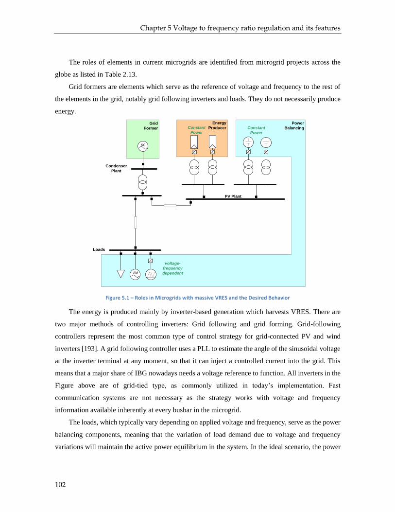
Chapter 5 Voltage to frequency ratio regulation and its features
102
The roles of elements in current microgrids are identified from microgrid projects across the
globe as listed in Table 2.13.
Grid formers are elements which serve as the reference of voltage and frequency to the rest of
the elements in the grid, notably grid following inverters and loads. They do not necessarily produce
energy.
SC
Condenser
Plant
PV Plant
Loads
AM
Grid
Former
Energy
ProducerPower
BalancingConstant
Power
voltage-
frequency
dependent
Constant
Power
Figure 5.1 – Roles in Microgrids with massive VRES and the Desired Behavior
The energy is produced mainly by inverter-based generation which harvests VRES. There are
two major methods of controlling inverters: Grid following and grid forming. Grid-following
controllers represent the most common type of control strategy for grid-connected PV and wind
inverters [193]. A grid following controller uses a PLL to estimate the angle of the sinusoidal voltage
at the inverter terminal at any moment, so that it can inject a controlled current into the grid. This
means that a major share of IBG nowadays needs a voltage reference to function. All inverters in the
Figure above are of grid-tied type, as commonly utilized in today’s implementation. Fast
communication systems are not necessary as the strategy works with voltage and frequency
information available inherently at every busbar in the microgrid.
The loads, which typically vary depending on applied voltage and frequency, serve as the power
balancing components, meaning that the variation of load demand due to voltage and frequency
variations will maintain the active power equilibrium in the system. In the ideal scenario, the power

Chapter 5 Voltage to frequency ratio regulation and its features
103
generation is independent of voltage and frequency, meaning that only the loads will decrease their
active power consumption when the active power production drops due to the intermittency.
The proposed regulation method guarantees the stability for microgrids operating with massive
levels of variable renewable based sources. The key points are:
Controlling the source voltage (V) and the frequency (f) in such a way as to keep the ratio
V/f essentially constant. This is performed by the grid formers
Granting the power equilibrium based on the self-adjusting characteristics of loads, thanks to
their dependence on the applied voltage and frequency.
Suitability with massive levels of DER (up to 100%), with today grid-tied inverter technology
without the need of storage systems
This strategy is therefore capable of providing smooth transition from classical grids to future
grids, considering the elements in the existing grids dominated by electrical machinery (transformers,
motors, generators, etc.) and the power-electronics dominated future grids (batteries, VRE, static
machines). Here, it is imagined that the priority is to go green and to acquire affordable microgrid,
both in its construction and operation phases. If better power quality is deemed to be necessary in
the future, upgrades can be made accordingly. The concept is introduced in Subsection 4.4.3.
The impact of voltage and frequency variations on active power consumption in a typical
residential microgrid in Indonesia is illustrated in Figure 5.2. The load model is depicted in Figure
2.12, the load proportions are taken from [242], while the ZIP and frequency-dependency coefficients
from [90], [91]. They are considered adequate for the purpose of our research. Newer research on ZIP
coefficient exists, such as in [243], where the load consumption is still typically found to decrease as
the voltage drops. The same behavior is also detected with frequency drop [34], [176] typically at 1-
2.5% per hertz.
Table 5.2 – Load proportion and coefficients in a typical residential microgrid in Indonesia
Load Pro-
portion p1 p2 p3 q1 q2 q3 Kpf
CFL Bulb 15% -0.03 1.66 -0.63 -0.06 1.4 -0.34 1
Incandescent Light
5% -0.04 0.5 0.54 0.03 0.51 0.46 0
Sodium Lamp 5% -0.04 1.2 -0.16 1.85 -4.11 3.26 0
Fan 15% -0.16 0.9 0.26 -0.12 0.62 0.5 1
LCD TV 14% 1.24 -0.57 0.33 15.22 -33.22 19 0
Refrigerator 29% 4.45 -8.48 5.03 12.18 -28.62 17.44 0.5
Rice Cooker 12% -0.02 0.1 0.92 -0.01 0.86 0.15 0
Washing Machine
5% 1.07 -0.84 0.77 6.56 -13.65 8.09 0.1

Chapter 5 Voltage to frequency ratio regulation and its features
104
Figure 5.2 – Impact of terminal voltage and/or frequency on a typical residential microgrid
As shown in Figure 5.2, optimum reduction of power consumption occurs when both frequency
and voltage are decreased. This action also exhibits supplementary benefits, as the ratio of voltage
and frequency is maintained at around unity, which satisfies the overfluxing limitations of the
electrical machinery devices. It should be noted that voltage reduction without frequency reduction
(also known as brownout) is authorized by some grid codes and is effective to shave the load in low
active power reserves [241]. However, it may be associated with stalling problems on induction
motors. On the other hand, frequency reduction without voltage reduction increases the V/f ratio
which may harm electrical machinery devices at excessive values. A number of grid codes and
standards require that the V/f ratio shall be maintained less than 1.1 in per unit [116], [182]. Other
consequences associated with the V/f strategy are discussed in more detail in Subsection 5.3.
It should also be clear that this strategy works if the load demand is dependent on voltage and
frequency variations. Consequently, constant power loads (already known to be demanding in
classical grids [244]) are onerous and huge proportion of this type of load in the microgrid may cause
this strategy to fail.
0.7
0.75
0.8
0.85
0.9
0.95
1
1.05
0.7 0.75 0.8 0.85 0.9 0.95 1 1.05
Act
ive
Po
we
r (p
.u.)
Voltage and/or Frequency (p.u.)
V and f variation
V variation
f variation

Chapter 5 Voltage to frequency ratio regulation and its features
105
The main benefits of this strategy are twofold. Firstly, the use of storage elements for stability
purposes can be minimized. A local use of storage only for very important loads is of course possible.
Secondly, fast communication systems are not necessary, as the frequency, a global system variable,
is used. When the microgrid is small, the voltage drop is small hence the voltage is ultimately uniform.
However, if the microgrid comprises long lines such that the voltage drop may be significant, several
grid formers (note that they do not have to produce energy) may be installed at several points in the
grid.
The new concept is proposed based on the fact that power consumption in a grid is dependent
and sensitive to voltage and frequency variations. Varying the voltage can be performed in short time
even in classical grids based on synchronous machine technology because this action typically does
not involve slow mechanical process. The voltage is reduced accordingly so as to maintain the power
equilibrium and the voltage to frequency ratio. The loads react in a solidary manner to reduce their
active power consumption upon frequency and voltage variations.
This strategy provides additional time for the grid operator and costumers to react to power
equilibrium occurring within the microgrid, as illustrated in Figure 5.3. Corrective actions such as
manual load disconnection or the activation of non-spinning reserves can be done if deemed
necessary. It should be noted that the system operates in mode “Potentially stable, demand response
necessary” based on the new proposed indices of stability in Table 3.5. Demand response is then
applied through V/f regulation to the loads, assuming that the loads are all solidary.
Cla
ssic
al R
eg
ula
tio
nV
/f R
eg
ula
tio
n TimeNormal Degraded
Alert
Normal
RestorativeIn extremis
(time sensitive)
Frequency keeps
decreasing, tripping,
islanding
(tolerant to time delays)
V/f to a new state
(tolerant to time delays)
Actions from customers
or grid operators
Actions from grid
operators
Normal voltage and
frequency, N-1 not
satistied
Normal voltage and
frequency, N-1 not
satistied
perturbation
Figure 5.3 – Comparison of traditional regulation vs V/f regulation when N-1 criterion in power generation is not
satisfied
This patent-pending concept [245] aims to preserve power system stability upon sudden decrease
due to the intermittency of VRES. The strategy has never been used for this specific purpose of

Chapter 5 Voltage to frequency ratio regulation and its features
106
maintaining production and consumption equilibrium in any other study prior to this research. With
regard to Figure 2.9, this concept is positioned within the evolution framework, where the changes
are transformative and incremental. We should keep in mind that the goal here is to transfer the
available power and to maintain the power balance at any instant.
5.2.2. Implementation on Synchronous Condenser
The proposed V/f strategy can be implemented on the grid forming elements, such as on
synchronous machines (including synchronous condensers) and grid forming inverters. It should be
noted that the reactive power injection strategy on grid supporting inverters may also need
adjustments due to the implementation of the strategy, as lower terminal voltage does not necessarily
mean reactive power insufficiency anymore, as discussed in Subchapter 5.4.
Key points of the implementation of the proposed regulation strategy are as follows.
Provided that the power variation is within the limit of power reserve, the system follows
the classical regulation (droop). A number of grid-supporting inverters function with
droop regulation.
If the power variation is larger than the power reserve, the V/f regulation varies the
voltage to achieve a new stable operating point
A modification on the input of the classical AVR is necessary in the implementation of the V/f
strategy on synchronous machines, such as depicted in Figure 5.4. The main variables include the
measured voltage u, the measured frequency frequency, and the excitation voltage uerrs. The voltage
setpoint input in the classical AVR, named u_setpoint in the diagram, is replaced with the measured
frequency, named frequency in the diagram. The objective here is to maintain the value of the terminal
voltage identical to the frequency.
xexr
012
3
K/sKI
012
3
sK/(1+sT)KD,TD
KKP
012
3-
012
3
012
3
-
012
3
Se(Efd)E1,Se1,E2,Se2
KKe
{1/sTTe
0.0
{K/(1+sT)}Ka,Ta
VRMAX
VRMIN
1/(1+sT)Tr
Vb
ias
avrr
ef
vs
voel
vuel
upss
de
r
integr duosvr
us
uek
vx
uerrs
pro
pu_setpoint
uru
frequency

Chapter 5 Voltage to frequency ratio regulation and its features
107
Figure 5.4 – Modification on AVR of synchronous machines (ESAC8B Model), V/f ratio = 1
If a variable V/f value is desired, a further modification is necessary, as depicted in Figure 5.5.
A new input of the voltage-to-frequency ratio VF_setpoint is added. Here, the target voltage is
maintained to be equal to the multiplication of the frequency and the V/f ratio setpoint.
xexr
012
3
K/sKI
012
3
sK/(1+sT)KD,TD
KKP
012
3-
012
3
012
3
-
012
3
Se(Efd)E1,Se1,E2,Se2
KKe
{1/sTTe
0.0
{K/(1+sT)}Ka,Ta
VRMAX
VRMIN
1/(1+sT)Tr
o1
VF_setpoint
Vb
ias
avrr
ef
vs
voel
vuel
upss
de
r
integr duosvr
us
uek
vx
uerrs
pro
p
frequency
uru
Figure 5.5 – Implementation of V/f strategy on synchronous machine’s AVR (ESAC8B Model), changeable V/f ratio
The implementation of the V/f regulation on synchronous condensers impacts the voltage
regulation. The simplified signal connection between the synchronous condenser and the voltage
controls is depicted in Figure 5.6. It is noteworthy to recall that the governor is non-existent in this
technology. As explained in Subchapter 5.2.1, in the V/f strategy, grid formers are not required to
produce energy. They serve as the voltage and frequency references and are temporarily responsible
for power balancing during transient period. This task is possible with synchronous condensers thanks
to their mechanical inertia.

Chapter 5 Voltage to frequency ratio regulation and its features
108
(a)
(b)
Figure 5.6 – Implementation of V/f strategy on Synchronous Condenser as a grid former (a) classical AVR (b) V/f regulation
This strategy is self-regulating, as the controls will adjust the terminal voltage until the frequency
is stable, meaning the power equilibrium is achieved. It should be noted that the exciter’s apparent
power rating is typically less than 0.5% of the rating of the synchronous condenser. The voltage to
frequency ratio is maintained around 1, however the exact value may vary depending on several
considerations, such as reactive power sharing among grid formers, voltage setpoint at nominal
operating condition, and load behavior. In practice, the frequency can be acquired based on the
measurement of the rotor speeds.
According to current design rules, generators may go as low as 0.9 pu in voltage while
maintaining the nominal frequency. With the V/f strategy, the voltage should be allowed to drop even
lower, but the voltage to frequency ratio shall be maintained so as to avoid overheating and damage
to electrical machinery. Special signals with slow communication systems may be employed for
setpoint setting purposes, for example for setting the voltage setpoint or to send out certain signals to
customers or directly to the devices.
Analyses such as time domain simulations may be necessary to confirm the microgrid stability
with this strategy. In this research, the reference test cases common in the industry are utilized to test
the proposed strategy. From the simulations with typical microgrids, it is found that the synchronous
condensers should be rated around 15-25% of the peak load in order to maintain a stable frequency.
5.2.3. Implementation on Grid Forming Inverter
The V/f concept can also be implemented on grid forming inverters, such as on virtual
synchronous machine (VSM)-like elements. Here, the element is said to be VSM-like (and not VSM)
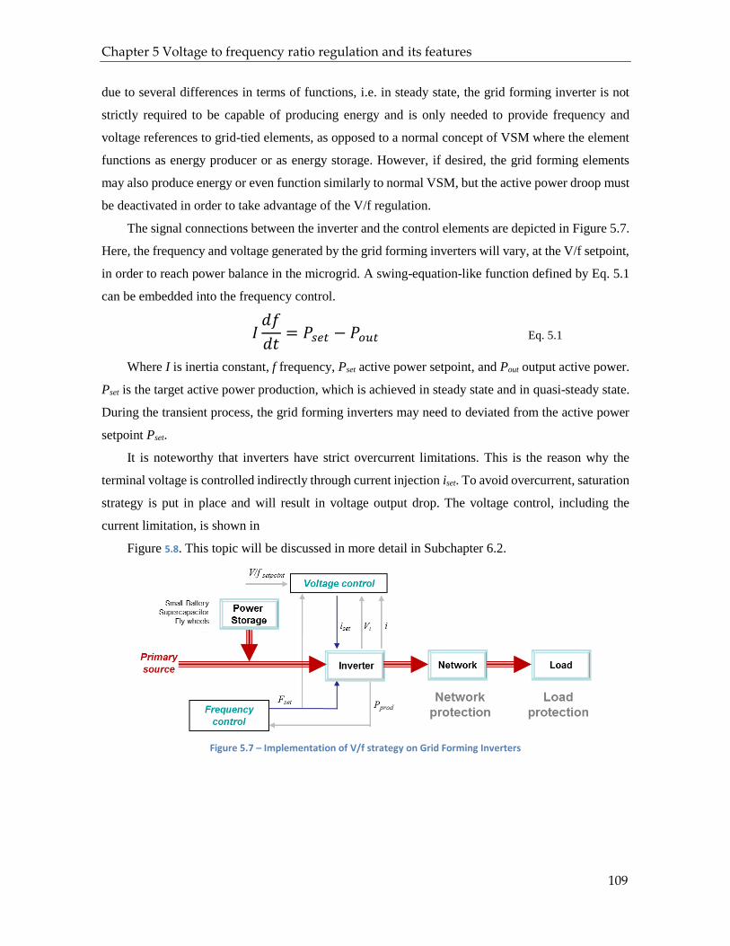
Chapter 5 Voltage to frequency ratio regulation and its features
109
due to several differences in terms of functions, i.e. in steady state, the grid forming inverter is not
strictly required to be capable of producing energy and is only needed to provide frequency and
voltage references to grid-tied elements, as opposed to a normal concept of VSM where the element
functions as energy producer or as energy storage. However, if desired, the grid forming elements
may also produce energy or even function similarly to normal VSM, but the active power droop must
be deactivated in order to take advantage of the V/f regulation.
The signal connections between the inverter and the control elements are depicted in Figure 5.7.
Here, the frequency and voltage generated by the grid forming inverters will vary, at the V/f setpoint,
in order to reach power balance in the microgrid. A swing-equation-like function defined by Eq. 5.1
can be embedded into the frequency control.
𝐼𝑑𝑓
𝑑𝑡= 𝑃𝑠𝑒𝑡 − 𝑃𝑜𝑢𝑡 Eq. 5.1
Where I is inertia constant, f frequency, Pset active power setpoint, and Pout output active power.
Pset is the target active power production, which is achieved in steady state and in quasi-steady state.
During the transient process, the grid forming inverters may need to deviated from the active power
setpoint Pset.
It is noteworthy that inverters have strict overcurrent limitations. This is the reason why the
terminal voltage is controlled indirectly through current injection iset. To avoid overcurrent, saturation
strategy is put in place and will result in voltage output drop. The voltage control, including the
current limitation, is shown in
Figure 5.8. This topic will be discussed in more detail in Subchapter 6.2.
Figure 5.7 – Implementation of V/f strategy on Grid Forming Inverters
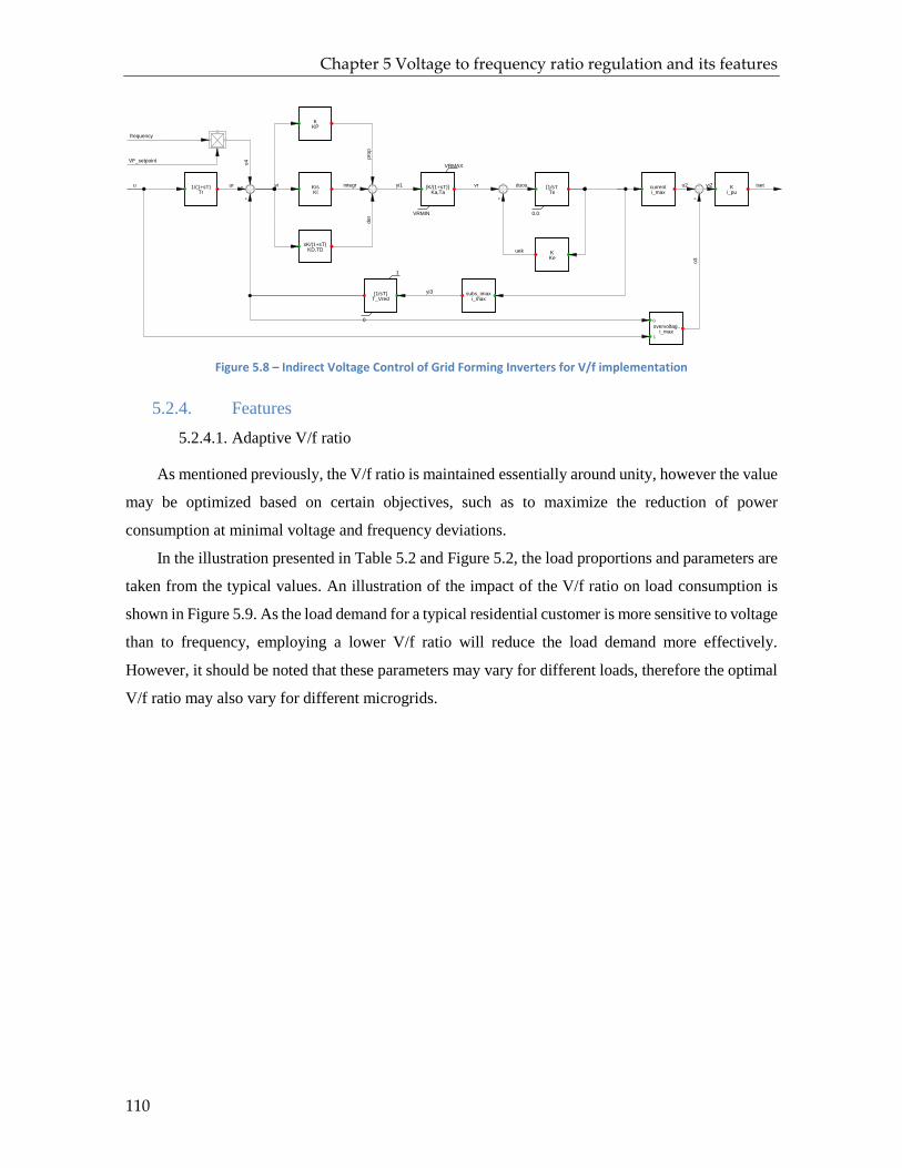
Chapter 5 Voltage to frequency ratio regulation and its features
110
0
1
overvoltag..i_max
012
3
-
subs_imaxi_max
[1/sT]T_Vred
1
0
currenti_max
Ki_pu
012
3012
3-
-
[K/(1+sT)]Ka,Ta
VRMAX
VRMIN
sK/(1+sT)KD,TD
K/sKI
KKP
KKe
[1/sTTe
0.0
012
3
-
1/(1+sT)Tr
o4VF_setpoint
frequency
yi2
o3
o2
yi3
iset
uek
duosvryi1
pro
pd
er
integryiuru
Figure 5.8 – Indirect Voltage Control of Grid Forming Inverters for V/f implementation
5.2.4. Features
5.2.4.1. Adaptive V/f ratio
As mentioned previously, the V/f ratio is maintained essentially around unity, however the value
may be optimized based on certain objectives, such as to maximize the reduction of power
consumption at minimal voltage and frequency deviations.
In the illustration presented in Table 5.2 and Figure 5.2, the load proportions and parameters are
taken from the typical values. An illustration of the impact of the V/f ratio on load consumption is
shown in Figure 5.9. As the load demand for a typical residential customer is more sensitive to voltage
than to frequency, employing a lower V/f ratio will reduce the load demand more effectively.
However, it should be noted that these parameters may vary for different loads, therefore the optimal
V/f ratio may also vary for different microgrids.

Chapter 5 Voltage to frequency ratio regulation and its features
111
Figure 5.9 – Impact of V/f ratio on active power demand in a typical residential microgrid
5.2.4.2. Indicator of underproduction
Instead of using fast and costly communication systems to send out command signals in typical
microgrid regulation strategy, slower to no-communication systems can be employed in the V/f
strategy. This eases the power balance monitoring within the microgrid. We may imagine using
simple bulbs or fans as indicators of power balance which are directly accessible to customers, as the
brightness (for bulbs) and speed (for fan) will decrease when the active power production is lower
than the demand. The customers therefore can react based on this information to adjust their electricity
usage accordingly. For example, when the bulbs shine less brightly, this is an alarm that the system
is experiencing underproduction, and the customers can manually turn off their devices. This process
is not time sensitive, as long as the voltage and frequency deviations are acceptable to everybody in
the microgrid. In this regard, the customers are not only consumers anymore as they are becoming
actors who actively help manage the microgrid. Therefore the costumers can be said to become
consumactors. This concept has been successfully tested with real time hardware-in-the-loop (HIL)
experiments as discussed in Chapter 7.
0.65
0.7
0.75
0.8
0.85
0.9
0.95
1
1.05
0.65 0.7 0.75 0.8 0.85 0.9 0.95 1 1.05
Act
ive
Po
we
r D
em
and
(p
.u.)
Frequency (p.u.)
VF 1.05
VF 1
VF 0.95
VF 0.9

Chapter 5 Voltage to frequency ratio regulation and its features
112
The underproduction can be quantified by the microgrid operator from the measurement of
frequency and voltage with the knowledge of load behavior, for example the one presented in Figure
5.2 for a typical residential microgrid. From such information, the microgrid operator can obtain the
approximate active power required to bring the microgrid back to the normal operations, with respect
to the actual active power production. Then, the operator can react accordingly, for example by
starting a diesel generator set. Again, this process is not time-sensitive as long as the frequency and
voltage deviations are accepted.
5.2.4.3. Multiple grid formers
Although microgrids typically have short power lines [68], certain types of microgrids may cover
wider area and hence longer power lines, such as the case in developing countries [94]. This condition
means that the voltage-to-frequency ratio may differ at different locations within the microgrid due
to the voltage drop. Furthermore, single non-redundant grid forming element is rather risky to the
grid operation, as its failure will cause a grid-wide blackout. In this proposed V/f strategy, multiple
grid forming elements can be installed at different points within the microgrid. They are responsible
for maintaining local voltage-to-frequency ratio. Here, the term “local” applies to the area electrically
close to the grid former such that the voltage drop is negligible.
5.2.4.4. System mitosis
Here, mitosis is defined as a process in which a microgrid is further split into a number of smaller
grids. Each smaller grid is independent of one another and has to possess energy producing elements,
loads, and at least one grid forming element. The mitosis typically results in several grids operating
at different frequency and voltage in post-disturbance quasi steady state. A typical mitosis is
illustrated in Subchapter 6.1.4.
However, anti-mitosis strategies are yet to be explored as the exact reverse of mitosis without
proper coordination may lead to very high transient current that will harm the transition.
5.3. Consequences of the larger voltage and frequency deviations in V/f
strategy
The implementation of the V/f strategy brings along a number of consequences for microgrid
operation and for the components in the microgrid, as higher deviations of frequency and voltage in
the grid are intentionally authorized. They impact a number of grid operations, as follows.
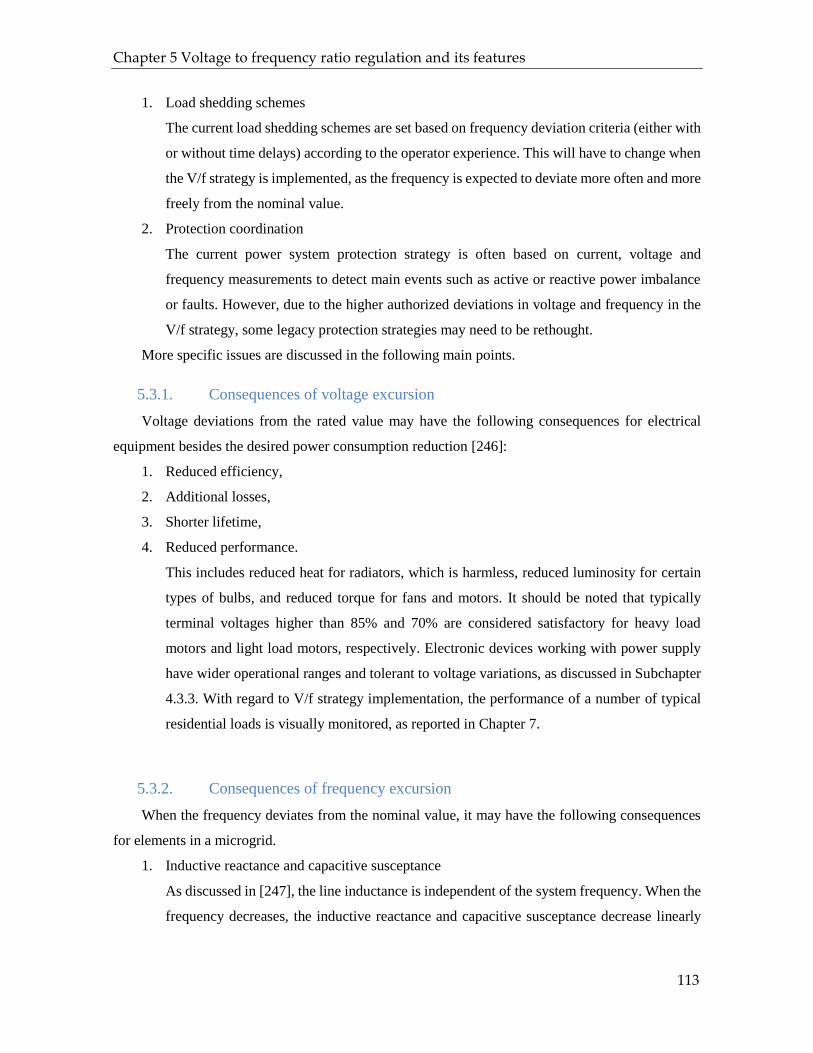
Chapter 5 Voltage to frequency ratio regulation and its features
113
1. Load shedding schemes
The current load shedding schemes are set based on frequency deviation criteria (either with
or without time delays) according to the operator experience. This will have to change when
the V/f strategy is implemented, as the frequency is expected to deviate more often and more
freely from the nominal value.
2. Protection coordination
The current power system protection strategy is often based on current, voltage and
frequency measurements to detect main events such as active or reactive power imbalance
or faults. However, due to the higher authorized deviations in voltage and frequency in the
V/f strategy, some legacy protection strategies may need to be rethought.
More specific issues are discussed in the following main points.
5.3.1. Consequences of voltage excursion
Voltage deviations from the rated value may have the following consequences for electrical
equipment besides the desired power consumption reduction [246]:
1. Reduced efficiency,
2. Additional losses,
3. Shorter lifetime,
4. Reduced performance.
This includes reduced heat for radiators, which is harmless, reduced luminosity for certain
types of bulbs, and reduced torque for fans and motors. It should be noted that typically
terminal voltages higher than 85% and 70% are considered satisfactory for heavy load
motors and light load motors, respectively. Electronic devices working with power supply
have wider operational ranges and tolerant to voltage variations, as discussed in Subchapter
4.3.3. With regard to V/f strategy implementation, the performance of a number of typical
residential loads is visually monitored, as reported in Chapter 7.
5.3.2. Consequences of frequency excursion
When the frequency deviates from the nominal value, it may have the following consequences
for elements in a microgrid.
1. Inductive reactance and capacitive susceptance
As discussed in [247], the line inductance is independent of the system frequency. When the
frequency decreases, the inductive reactance and capacitive susceptance decrease linearly

Chapter 5 Voltage to frequency ratio regulation and its features
114
and their variations may need to be taken into account in the calculations if deemed
necessary.
2. Generators
Frequency drop may be problematic to generators. Cooling systems are running below
normal speed. If the AVR is controlled to maintain the terminal voltage, there is a risk of
overfluxing. The thermal power plant output decreases because the blast of the cooling fans
decreases, causing a reduced output.
3. Turbines
Steam turbine technology is used to convert steam to electric power. The blades of a steam
turbine have several natural frequencies associated with higher mechanical stresses. High
deviation of frequency thus causes the turbine to work closer to these hazardous regions of
operation. The damage is rather cumulative. Underfrequency events are generally more
stressful. Typically the concern is when the frequency deviates more than about 5% [248].
On the other hand, frequency deviation shows no meaningful impacts on hydraulic turbines
[249].
4. Generator protection
Relays based on ROCOF are often installed on distributed generations to keep them from
running in an unintended island. High levels of ROCOF in combinations with improper
settings can thus cause disconnections of DGs which will worsen the situation in
underfrequency situations.
5. Auxiliary systems
Auxiliary systems providing services such as cooling, feeding, and fans are normally
coupled with induction machines. Their performance, especially speed, will decrease as the
frequency drops.
6. Flux Density of electrical machinery components
Most components of a power system are electrical machinery, functioning based on magnetic
material. They are sensitive to the flux density passing through them, which is directly
proportional to voltage and inversely proportional to frequency [248], [250]. Violation of
the flux density limit may cause heat losses and saturation of magnetic core.
7. Industrial loads
Poor power system frequency controls may degrade the power quality [248]. However, the
power quality impacts of frequency variations are somewhat unclear. Most industrial
processes which are sensitive to frequency variations have variable frequency drives which
are normally insensitive to frequency disturbances.

Chapter 5 Voltage to frequency ratio regulation and its features
115
8. Clocks
Clocks that depend on the supply frequency will be affected [251]. For example, the clocks
would be off by about two minutes every hour for a deviation of 2 Hz from the nominal
value.
5.3.3. Further Discussion on the Consequences of the V/f strategy
In discussions about frequency and voltage variations and their effects on equipment, the V/f
ratio is always brought up as a potential risk that requires attention. When the V/f ratio is kept
constant, electrical machinery such as induction motors can operate successfully [252]. For frequency
variation up to 50% of the nominal value, the starting torque capability does not change much and
the motors are still able to provide the full rated load torque, as shown in Figure 5.10. However,
prolonged voltage and frequency variations on induction motors may still result in winding
temperature increase, even at constant flux density [253]. This happens due to several reasons, such
as reduced fan speed influencing the cooling systems.
Starting
torque
Pullout
torque
Full-load
torque
Figure 5.10 – Torque-speed characteristic curves for speeds below base speed (nominal speed at 1800 rpm), line voltage is derated linearly with frequency [250]
With respect to the voltage nose point often discussed in voltage stability, voltage reductions
may bring the nose point closer, meaning that the voltage collapse occurs at a lower loading level. On

Chapter 5 Voltage to frequency ratio regulation and its features
116
the other hand, frequency reductions will decrease the reactance, which will result in the nose point
shifting to the right, yielding more voltage stability. The phenomena are illustrated in Figure 5.12.
The simulation is performed on a simplified system depicted in Figure 5.11 for a constant load power
factor of 0.9 lagging. In order to obtain realistic conditions in distribution systems, the R/X ratio of
the system impedance is assumed to be relatively high, at 0.66.
ZTÐqT
ZLÐqLVs
Vr
P + jQ
Figure 5.11 – Simplified system for P-V curve construction
In Figure 5.11 above, Vs is the source voltage, ZT the transmission impedance, Vr the voltage at
load terminal, P the load active power, Q the load reactive power, and ZL the load impedance.
0 0.2 0.4 0.6 0.8 1 1.2
P/Pmax
0
0.1
0.2
0.3
0.4
0.5
0.6
0.7
0.8
0.9
1
Vr
Vs = 1 p.u., f = 1 p.u.
Vs = 1 p.u., f = 0.9 p.u.
Vs = 0.9 p.u., f = 1 p.u.
Figure 5.12 – PV Curves illustrating voltage stability changes either due to voltage or frequency variation
In Figure 5.12, Vr is the receiving voltage, while Pmax is the maximum active power transfer at
nominal voltage and frequency.
When frequency and voltage variations are intentionally done simultaneously, the resulting P-V
curve is shown in Figure 5.13 (a). It is noticeable that the nose-point of the P-V curve when both the
voltage and frequency are reduced is located in the right side of that when only the voltage is
decreased.

Chapter 5 Voltage to frequency ratio regulation and its features
117
Let us study the impact of load increase when there are no available primary reserves. This is
illustrated in Figure 5.13 (b). P1(V,f) and P2(V,f) are active power consumption characteristics of the
loads, which are functions of the terminal voltage and the system frequency. The operating point is
initially at t0. A load impact then occurs, normally shifting the operating point to t1. However, as no
primary reserves are available, the V/f strategy reacts by decreasing the voltage and the frequency
simultaneously, bringing the operating point to t3, where the final active power demand is the same
as the initial one. In this case, the final operating point is at Vs = 0.9 p.u. and f = 0.9 p.u. The resulting
loadability indices (defined by Eq. 3.10) of point t1 and t2 are comparable.
0 0.2 0.4 0.6 0.8 1 1.2
P/Pmax
0
0.1
0.2
0.3
0.4
0.5
0.6
0.7
0.8
0.9
1
Vr
Vs = 1 p.u., f = 1 p.u.
Vs = 0.9 p.u., f = 0.9 p.u.
(a)

Chapter 5 Voltage to frequency ratio regulation and its features
118
0 0.2 0.4 0.6 0.8 1 1.2
P/Pmax
0
0.1
0.2
0.3
0.4
0.5
0.6
0.7
0.8
0.9
1
Vr
Vs = 1 p.u., f = 1 p.u.
Vs = 0.9 p.u., f = 0.9 p.u.
P1(V,f) P2(V,f)
t0t1
t2
(b)
Figure 5.13 – Voltage stability changes due to the V/f strategy (a) Typical V(P) curves (b) operating point progress upon load increase
The final analysis on whether or not the microgrid becomes better in terms of voltage stability
with respect to the V/f strategy depends on several factors, such as the system impedance and the load
behavior. As discussed previously, voltage reductions will shift the nose point to the left while
frequency reductions will shift the nose point to the right due to the reactance drop.
As for the load behavior, the more the load is solidary to voltage and frequency deviations; the
better it is in terms of voltage stability. This is illustrated in Figure 5.14. Let us say that the initial
operating point at nominal voltage and frequency is at t0, very close to the nose point but is still in the
voltage-stable region. Upon a perturbation of total production drop from G0 to G1, the operating point
will move to a new stable operating point t1 if the load behavior follows the function P1(V,f). However,
if the load behavior follows the function P2(V,f), it does not cross the stable region regardless of the
V/f regulation strategy, therefore a new voltage-stable operating point cannot be achieved, and the
blackout is inevitable.
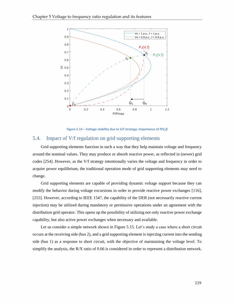
Chapter 5 Voltage to frequency ratio regulation and its features
119
0 0.2 0.4 0.6 0.8 1 1.2
P/Pmax
0
0.1
0.2
0.3
0.4
0.5
0.6
0.7
0.8
0.9
1
Vr
Vs = 1 p.u., f = 1 p.u.
Vs = 0.9 p.u., f = 0.9 p.u.
P1(V,f)t0
P2(V,f)
t1
t’1 G0G1
Figure 5.14 – Voltage stability due to V/f strategy: Importance of P(V,f)
5.4. Impact of V/f regulation on grid supporting elements
Grid supporting elements function in such a way that they help maintain voltage and frequency
around the nominal values. They may produce or absorb reactive power, as reflected in (newer) grid
codes [254]. However, as the V/f strategy intentionally varies the voltage and frequency in order to
acquire power equilibrium, the traditional operation mode of grid supporting elements may need to
change.
Grid supporting elements are capable of providing dynamic voltage support because they can
modify the behavior during voltage excursions in order to provide reactive power exchanges [116],
[255]. However, according to IEEE 1547, the capability of the DER (not necessarily reactive current
injection) may be utilized during mandatory or permissive operations under an agreement with the
distribution grid operator. This opens up the possibility of utilizing not only reactive power exchange
capability, but also active power exchanges when necessary and available.
Let us consider a simple network shown in Figure 5.15. Let’s study a case where a short circuit
occurs at the receiving side (bus 2), and a grid supporting element is injecting current into the sending
side (bus 1) as a response to short circuit, with the objective of maintaining the voltage level. To
simplify the analysis, the R/X ratio of 0.66 is considered in order to represent a distribution network.

Chapter 5 Voltage to frequency ratio regulation and its features
120
Zt
vs vr
1 2
Figure 5.15 – Schematic diagram of a simple two-bus network
The relations between the sending voltage vs, current injection into the sending bus is, and the
network impedance Zt is as follows.
𝑣𝑠 = 𝑣𝑟 + 𝑖𝑠 ∗ 𝑍𝑡 Eq. 5.2
Let us define
𝑣𝑠 = |𝐸1|∠𝛿𝑣
𝑣𝑟 = |𝐸2|∠0
𝑖𝑠 = |𝐼1|∠𝛿𝑖
𝑍𝑡 = |𝑍|∠𝜃𝑧
Therefore
|𝐸1|∠𝛿𝑣 = |𝐸2|∠0 + |𝐼1| ∗ |𝑍|∠(𝛿𝑖 + 𝜃𝑧) Eq. 5.3
Here, the impact of active power on the voltage is not negligible anymore due to the higher line
resistance. In order to visualize the impact of current injection on dynamic voltage support, the short
circuit is assumed to drop the voltage at the receiving bus to 0.3 per unit. Let us use the following per
unit values, derived while taking typical distribution network and inverter-based generation into
account:
𝑣𝑟 = 0.3∠0
|𝐼1| = 1
|𝑍| = 0.02
The impact of the angle of the current injection δi on the sending voltage at three different R/X
values is presented in Figure 5.16.

Chapter 5 Voltage to frequency ratio regulation and its features
121
-100 -80 -60 -40 -20 0 20 40 60 80 100
δi (degrees)
0.28
0.285
0.29
0.295
0.3
0.305
0.31
0.315
0.32
0.325
|E1| (p
.u.)
0
0.5
1
1.5
2
2.5
3
3.5
4
δv (
de
gre
es)
-100 -80 -60 -40 -20 0 20 40 60 80 1000.28
0.285
0.29
0.295
0.3
0.305
0.31
0.315
0.32
-2
-1
0
1
2
3
4
-100 -80 -60 -40 -20 0 20 40 60 80 1000.285
0.29
0.295
0.3
0.305
0.31
0.315
0.32
-3
-2
-1
0
1
2
3
4
(a) (b)
(c)
δi (degrees)
|E1| (p
.u.)
δv (
de
gre
es)
δi (degrees)
|E1| (p
.u.)
δv (
de
gre
es)
Figure 5.16 – Impact of current injection of grid supporting elements on PCC Voltage during short Circuit (a) system R/X =0 (b) system R/X = 0.578 (c) system R/X = 1
The power injection into the sending bus is the multiplication of the sending voltage and the
conjugate of the current injection. Consequently, the type of injected power can be known by
inspecting the angle difference between the sending voltage δv and current injection δi. In Figure 5.16
(a), the network is inductive, 𝜃𝑧 = 90°, and maximum sending voltage |E1| is achieved when the
angle difference sending voltage and injected current (δv - δi) is 90°, meaning the injected current is
completely reactive. Likewise, when the network’s R/X is 0.578 (𝜃𝑧 = 60°) and R/X is 1 (𝜃𝑧 = 45°),
the maximum sending voltage |E1| is achieved when the angle difference sending voltage and injected
current (δv - δi) is 60° and 45°, respectively, meaning that the injected current contains both active and
reactive parts. It is therefore found that the optimum dynamic voltage support is achieved when the
injected current’s angle with respect to the voltage angle at the PCC matches the angle of the network
impedance. This conclusion has been compared to other dynamic voltage support strategies with
simulations using real data in [256]. Nonetheless, the reported study only focuses on the voltage
aspect, neglecting the impact on frequency.

Chapter 5 Voltage to frequency ratio regulation and its features
122
When dealing with distribution networks and the V/f strategy, one has to consider the impact of
short-circuits on the frequency as well. As the grid former is not necessarily an energy producer and
the network is characterized by higher R/X values, the impact of the dynamic voltage support on the
power equilibrium during short-circuit, should be taken into consideration. This will also influence
the critical clearing time.
The network described in Figure 5.17 illustrates the issue. The V/f regulations are implemented
on all the grid formers, namely GF and the reference machine. The load’s active power demand and
the network losses are supplied solely by the energy producer in steady state. The reference machine
is assumed to have higher inertia constant compared to grid former GF. If a three-phase short circuit
with small fault impedance occurs at bus 2, the impacts of different dynamic voltage support strategies
are presented in Figure 5.18.
Energy
Producer
SC
SC
1 2
3
Re
fere
nce
Ma
ch
ine
2 MW
0.97 PF
6 MWp
GF
PV
Figure 5.17 – Simple network for dynamic voltage support study with the V/f strategy
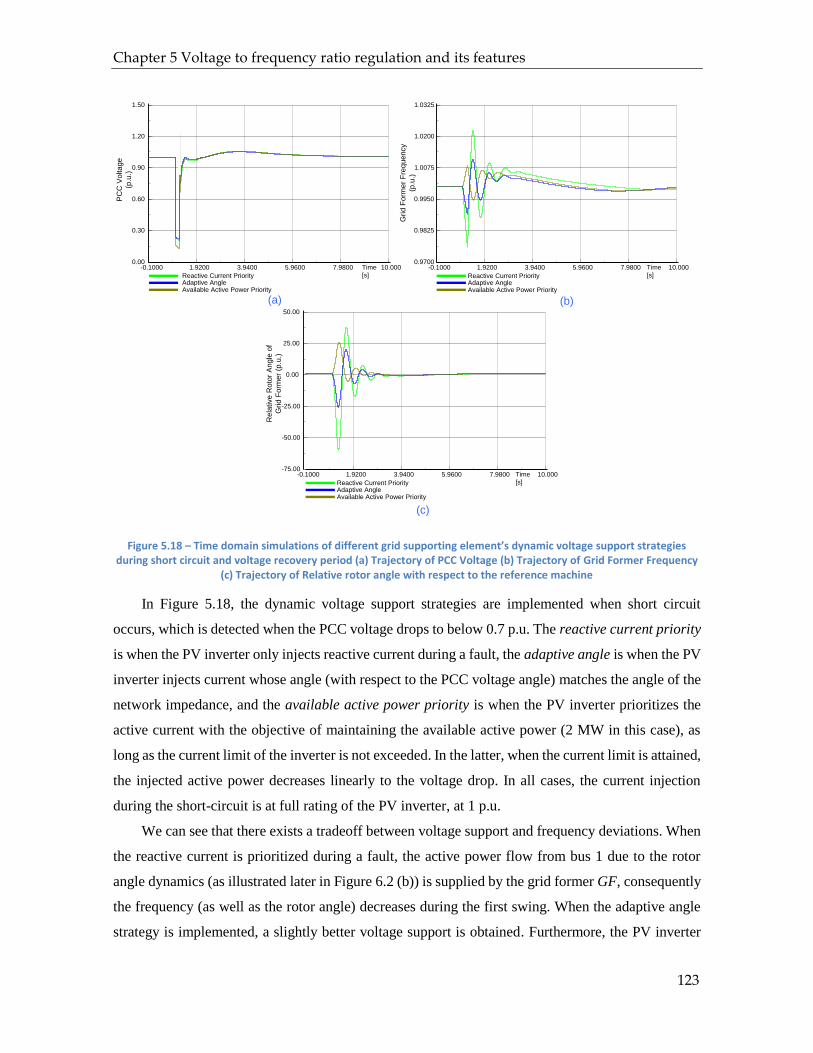
Chapter 5 Voltage to frequency ratio regulation and its features
123
10.000
10.0007.98005.96003.94001.9200-0.1000 Time
[s]
1.50
1.20
0.90
0.60
0.30
0.00
PC
C V
olta
ge
(p.u
.)
Reactive Current PriorityAdaptive AngleAvailable Active Power Priority
10.0007.98005.96003.94001.9200-0.1000
1.0325
1.0200
1.0075
0.9950
0.9825
0.9700
10.0007.98005.96003.94001.9200-0.1000
50.00
25.00
0.00
-25.00
-50.00
-75.00
Time
[s]
Grid
Fo
rme
r F
req
ue
ncy
(p.u
.)
Time
[s]
Re
lative
Ro
tor
An
gle
of
Grid
Fo
rme
r (p
.u.)
Reactive Current PriorityAdaptive AngleAvailable Active Power Priority
Reactive Current PriorityAdaptive AngleAvailable Active Power Priority
(a) (b)
(c)
Figure 5.18 – Time domain simulations of different grid supporting element’s dynamic voltage support strategies during short circuit and voltage recovery period (a) Trajectory of PCC Voltage (b) Trajectory of Grid Former Frequency
(c) Trajectory of Relative rotor angle with respect to the reference machine
In Figure 5.18, the dynamic voltage support strategies are implemented when short circuit
occurs, which is detected when the PCC voltage drops to below 0.7 p.u. The reactive current priority
is when the PV inverter only injects reactive current during a fault, the adaptive angle is when the PV
inverter injects current whose angle (with respect to the PCC voltage angle) matches the angle of the
network impedance, and the available active power priority is when the PV inverter prioritizes the
active current with the objective of maintaining the available active power (2 MW in this case), as
long as the current limit of the inverter is not exceeded. In the latter, when the current limit is attained,
the injected active power decreases linearly to the voltage drop. In all cases, the current injection
during the short-circuit is at full rating of the PV inverter, at 1 p.u.
We can see that there exists a tradeoff between voltage support and frequency deviations. When
the reactive current is prioritized during a fault, the active power flow from bus 1 due to the rotor
angle dynamics (as illustrated later in Figure 6.2 (b)) is supplied by the grid former GF, consequently
the frequency (as well as the rotor angle) decreases during the first swing. When the adaptive angle
strategy is implemented, a slightly better voltage support is obtained. Furthermore, the PV inverter

Chapter 5 Voltage to frequency ratio regulation and its features
124
helps compensate the active power transfer during short circuit, causing slower dynamics of GF rotor
angle and frequency. This indeed increases the critical clearing time of the grid former if the
synchronous condenser technology is chosen. When the available active power priority strategy is
employed, the voltage support is not as good, and the active power transfer during short circuit may
be overcompensated, resulting in rotor acceleration. In this simple case, the adaptive angle strategy
comes out as the best option, as it supports both the voltage during a short-circuit, and slows down
the rotor deceleration, which improves the critical clearing time of the grid forming element GF.
Nevertheless, this topic can be further developed, as the network R/X may vary for different fault
locations, and the power-angle curves during short circuits are a function of the remaining short circuit
voltage, the fault location, and the fault impedance. An optimization problem on the dynamic voltage
support strategy, taking into account the impact on both voltage and frequency, can be constructed,
which is an interesting future research topic to look into.
5.5. Possible Application in Microgrids
Besides in low-HDI areas previously living without electricity and in post-disaster relief
situations, the V/f regulation is suitable to be implemented for a number of other reasons in
microgrids, depending on the operational objectives. Several opportunities that we identified are as
follows.
1. Improving the efficiency and reducing the operation cost.
Even when diesel generators are available, the microgrid operators can opt not to operate
them just for dealing with the contingency events. This is a major improvement, especially
when the operator intends to operate at 100% of renewables most of the time, as the operation
of diesel generators at minimal loading is not efficient at all. In this regard, diesel generators
are only when needed when it is deemed so according to the situation (e.g. restoration of the
frequency and voltage to the nominal values, bad weather reasons). By employing the V/f
strategy, the operator acquires a new dimension of flexibility, i.e. time, without having to go
through the blackout state upon sudden reduction of renewable production.
2. Limitation of charge-discharge cycles of batteries
Batteries are limited in the number of charge-discharge cycles. This means that their
implementation in enhancing power system stability can be costly, as it requires frequent
operations. The V/f strategy can help reduce the number of battery operations, hence
optimizing the lifetime of the batteries and focusing the usage for energy balancing purposes.
3. Operation with limited storage systems (sizing benefits)

Chapter 5 Voltage to frequency ratio regulation and its features
125
As the V/f strategy (through the grid formers) can maintain the power equilibrium during
transient states, the power sizing of storage elements can be reduced, if desired.
4. Enhancing the last defense strategy
Working side-by-side with load shedding procedure, this strategy can be employed to avoid
frequent blackouts in microgrids, especially the ones operating in remote areas. As the
proposed strategy is compatible with the widely-used active power droop regulation, the
microgrid operation does not change much when the primary reserves are sufficient, which
will mean that the nominal frequency can be maintained in steady state. However, when an
unexpected event occurs, which will create high power imbalance, the V/f strategy will react
to maintain the power equilibrium within the microgrid and avoid the occurrence of
blackout. In this regard, the microgrid becomes more resilient, especially when the system
is dependent on batteries, which could be out of stored energy.
Furthermore, if power quality problems are considered important and the loads require power
conditioning, on-line UPS or solid state transformers can be utilized for a handful of loads, as a high
proportion of this type of load will cancel out the benefits of employing the V/f strategy. This has
been demonstrated in Sendai microgrid in Japan [257], [258], in which the loads are served at different
power quality through the use of an integrated power supply (see Figure 5.19). In this regard, the
loads connected through power conditioning elements will be seen as constant-power loads by the
microgrid.
Figure 5.19 – Single Line Diagram showing different classes of loads in Sendai Microgrid [258]
5.6. Conclusion
This chapter has provided clear explanation on the concept of voltage-to-frequency regulation
that we propose. In this concept, the elements in a microgrid can be categorized into three categories:

Chapter 5 Voltage to frequency ratio regulation and its features
126
grid forming element, energy producing element, and power balancer. The grid forming elements
function at zero active power in steady state. They maintain the stability of a microgrid so as to avoid
blackouts, making the microgrid more resilient. It should be noted that they still can work along with
continuous and discrete load shedding and local controls if desired.
As the current power systems mostly use electrical machinery, such as electric motors and
transformers, the overfluxing problem needs to be taken into account. This strategy ensures that the
voltage to frequency ratio is maintained around 1, ensuring that it does not harm the electrical
machinery. Furthermore, this strategy ensures the plug-and-play feature for newly connected energy
producing elements, loads, and grid forming elements. It is compatible with current grid-tied inverter
technologies and does not require fast communication systems. Still, possible future communication
upgrades can always be accommodated without problems. Finally, this proposed strategy is easy to
implement and does not require revolution in terms of power system equipment and control. Today’s
elements, such as electrical machinery and grid-tied inverters, are compatible with this approach. The
main drawback is that we have to accept higher deviations in voltage and frequency. In return, we
can accommodate massive level of VRES even at very low primary reserves, without communication
system, and we are given time flexibility to deal with power inequilibrium.
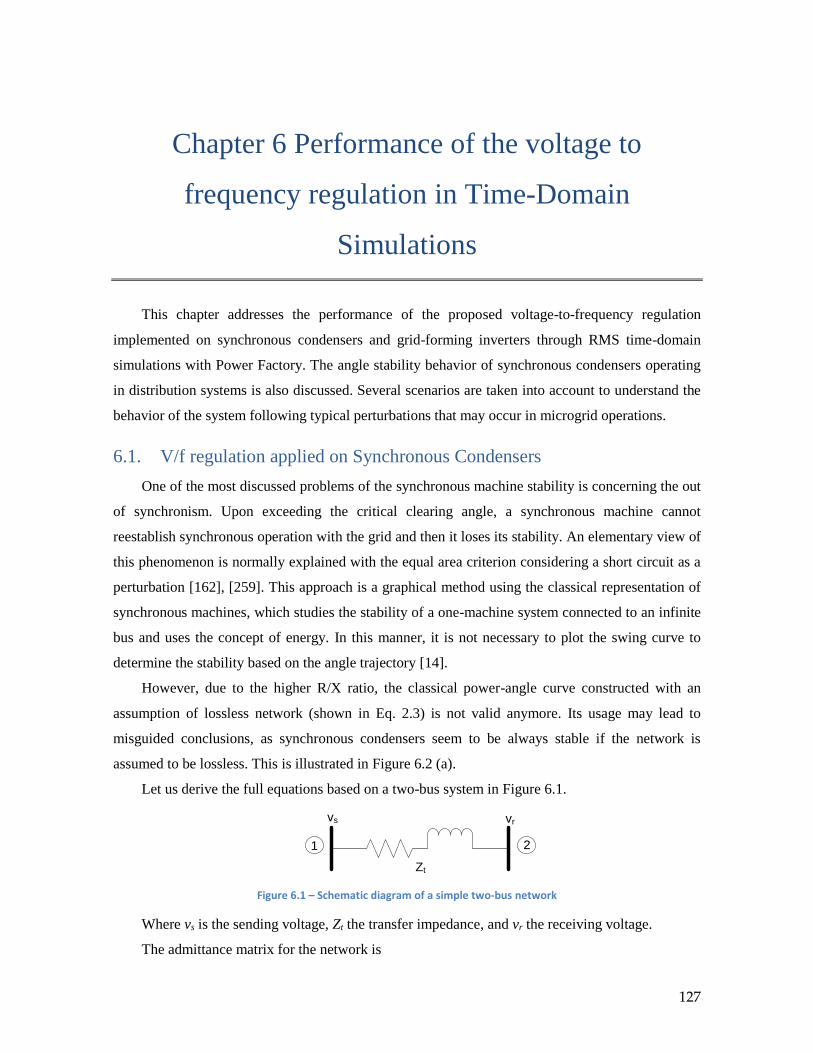
127
Chapter 6 Performance of the voltage to
frequency regulation in Time-Domain
Simulations
This chapter addresses the performance of the proposed voltage-to-frequency regulation
implemented on synchronous condensers and grid-forming inverters through RMS time-domain
simulations with Power Factory. The angle stability behavior of synchronous condensers operating
in distribution systems is also discussed. Several scenarios are taken into account to understand the
behavior of the system following typical perturbations that may occur in microgrid operations.
6.1. V/f regulation applied on Synchronous Condensers
One of the most discussed problems of the synchronous machine stability is concerning the out
of synchronism. Upon exceeding the critical clearing angle, a synchronous machine cannot
reestablish synchronous operation with the grid and then it loses its stability. An elementary view of
this phenomenon is normally explained with the equal area criterion considering a short circuit as a
perturbation [162], [259]. This approach is a graphical method using the classical representation of
synchronous machines, which studies the stability of a one-machine system connected to an infinite
bus and uses the concept of energy. In this manner, it is not necessary to plot the swing curve to
determine the stability based on the angle trajectory [14].
However, due to the higher R/X ratio, the classical power-angle curve constructed with an
assumption of lossless network (shown in Eq. 2.3) is not valid anymore. Its usage may lead to
misguided conclusions, as synchronous condensers seem to be always stable if the network is
assumed to be lossless. This is illustrated in Figure 6.2 (a).
Let us derive the full equations based on a two-bus system in Figure 6.1.
Zt
vs vr
1 2
Figure 6.1 – Schematic diagram of a simple two-bus network
Where vs is the sending voltage, Zt the transfer impedance, and vr the receiving voltage.
The admittance matrix for the network is

Chapter 6 Performance of the voltage to frequency regulation in Time-Domain Simulations
128
𝑌𝑏𝑢𝑠 =
(1) (2)(1)(2)
[𝑌11 𝑌12
𝑌21 𝑌22] Eq. 6.1
Where
𝑌11 = 1
𝑍𝑡 Eq. 6.2
𝑌12 = −1
𝑍𝑡 Eq. 6.3
As stated in [37], the power injection at bus 1 is given by the following equations.
𝑃1 + 𝑗𝑄1 = 𝑣𝑠(𝑌11𝑣𝑠)∗ + 𝑣𝑠(𝑌12𝑣𝑟)∗ Eq. 6.4
Let us define
𝑣𝑠 = |𝐸1|∠𝛿
𝑣𝑟 = |𝐸2|∠0
𝑌11 = 𝐺11 + 𝑗𝐵11
𝑌12 = |𝑌12|∠𝜃
Using the definitions above into Eq. 6.4 yields
𝑃1 = |𝐸1|2𝐺11 + |𝐸1||𝐸2||𝑌12| cos(𝛿 − 𝜃) Eq. 6.5
𝑄1 = −|𝐸1|2𝐵11 + |𝐸1||𝐸2||𝑌12| sin(𝛿 − 𝜃) Eq. 6.6
The angle 𝜃 is between 𝜋/2 and 𝜋. If we define
𝛾 = 𝜃 − 𝜋
2
Then we can derive that
𝑃1 = |𝐸1|2𝐺11 + |𝐸1||𝐸2||𝑌12| sin(𝛿 − 𝛾) Eq. 6.7
𝑄1 = −|𝐸1|2𝐵11 + |𝐸1||𝐸2||𝑌12| cos(𝛿 − 𝛾) Eq. 6.8
If we assume that the R/X ratio is 0.66 to simulate an actual distribution network, the resulting
power-angle curves based on Eq. 6.7 are presented in Figure 6.2 (b).

Chapter 6 Performance of the voltage to frequency regulation in Time-Domain Simulations
129
-200 -100 0 100 200 300 400
delta (degrees)
-1
-0.8
-0.6
-0.4
-0.2
0
0.2
0.4
0.6
0.8
1
P/P
ma
x
Normal Operation
Short Circuit
-200 -100 0 100 200 300 400
delta (degrees)
-0.4
-0.2
0
0.2
0.4
0.6
0.8
1
P/P
ma
x
Normal Operation
Short Circuit
(a) (b)
Figure 6.2 – Rotor Response superimposed on Power Angle Curve (a) lossless network (b) distribution network
If the network is assumed to be lossless, the power-angle curve follows the blue line in Figure
6.2 (a) in normal condition. The initial angle difference between the sending bus and the receiving
bus is zero, as the synchronous condenser does not inject active power to the network in steady state.
If a symmetrical short circuit occurs at bus 2, the power-angle follows the orange line. From the curve,
the synchronous condenser does not inject or absorb any active power to/from the grid, hence no
acceleration or deceleration. Therefore, the synchronous condenser appears to be always stable
regardless of the fault duration.
The assumption of lossless network could be misleading for the application on medium voltage
network. As depicted in Figure 6.2 (b), the power-angle curve follows the blue line in normal
condition. Initially, the angle difference is also zero as the synchronous condenser does not inject
active power. However, when a symmetrical short circuit at bus 2 is taking place, the power-angle
curve follows the orange line. In this state, the synchronous condenser injects active power to the
faulty grid, causing rotor deceleration. After the clearance of the fault, the power-angle curve returns
to the blue line, which shows that the synchronous condenser is now absorbing power from the grid.
If the energy released during the short circuit (depicted by the shaded light blue area) is equal to the
absorbed energy during the post-short circuit state (depicted by the shaded green area), the
synchronous condenser can reestablish synchronism with the grid. However, if the shaded light blue
area is smaller than the shaded green one, the synchronous condenser will continue to suffer from
deceleration and end up losing the synchronism.
This clearly illustrates that a stability limit of synchronous condensers still exists. In a sense,
equal-area criterion is still useful to describe the phenomenon. However, the issue here is rotor
deceleration, as opposed to the rotor acceleration often occurring in the first swing of synchronous

Chapter 6 Performance of the voltage to frequency regulation in Time-Domain Simulations
130
generators. It should be noted that the power-angle characteristic during short circuit (the orange line)
is affected by several factors, such as fault impedance and location.
These findings have been verified with time domain simulations with Digsilent Power Factory,
as shown in Figure 6.3. When the network is not considered lossless, out-of-synchronism can be
detected and if this happens, the synchronous condenser continues to decelerate even after short
circuit clearance.
5.00003.98002.96001.94000.9200-0.1000 Time
[s]
1.01
0.99
0.97
0.95
0.93
0.91
Speed
[p.u.]
Lossless NetworkDistribution Network
5.00003.98002.96001.94000.9200-0.1000 Time
[s]
300.00
200.00
100.00
0.00
-100.00
-200.00
Rotor
Angle
[deg]
Lossless NetworkDistribution Network
(a) (b)
Figure 6.3 – Time domain Rotor Response with respect to reference angle following a 500ms short circuit at t=1s (a) Rotor Angle (b) Rotor Speed
It is therefore found that the out of synchronism phenomenon still exists for synchronous
condensers in distribution networks. In the first swing, they suffer from rotor deceleration for the
application in distribution grids. Consequently, indices such as critical clearing angle and critical
clearing time are still useful.
In the following discussions, the V/f strategy is implemented on synchronous condensers, which
serve as the grid forming elements. The grid-tied inverters, which include grid-supporting battery and
PV systems, are modeled based on Schneider Electric’s Conext Series [260], [261] and considered
adequate for the purpose of this study. The battery inverters are capable of providing dynamic voltage
support and frequency support based on droop strategy, while the PV inverters possess similar
capabilities, however the active power droop only applies for overfrequency (active power
curtailment), as the PVs do not have primary reserves by default. The inverters possess circular
capability curves, as illustrated in Figure 5.13.
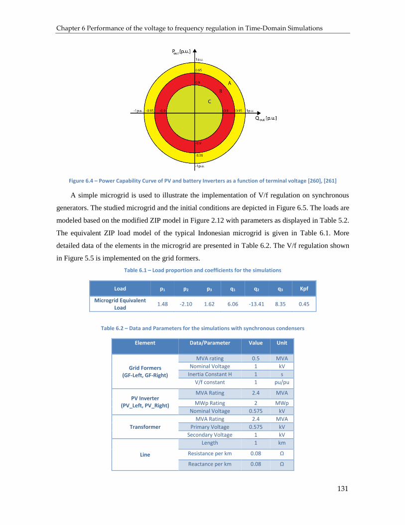
Chapter 6 Performance of the voltage to frequency regulation in Time-Domain Simulations
131
Figure 6.4 – Power Capability Curve of PV and battery Inverters as a function of terminal voltage [260], [261]
A simple microgrid is used to illustrate the implementation of V/f regulation on synchronous
generators. The studied microgrid and the initial conditions are depicted in Figure 6.5. The loads are
modeled based on the modified ZIP model in Figure 2.12 with parameters as displayed in Table 5.2.
The equivalent ZIP load model of the typical Indonesian microgrid is given in Table 6.1. More
detailed data of the elements in the microgrid are presented in Table 6.2. The V/f regulation shown
in Figure 5.5 is implemented on the grid formers.
Table 6.1 – Load proportion and coefficients for the simulations
Load p1 p2 p3 q1 q2 q3 Kpf
Microgrid Equivalent Load
1.48 -2.10 1.62 6.06 -13.41 8.35 0.45
Table 6.2 – Data and Parameters for the simulations with synchronous condensers
Element Data/Parameter Value Unit
Grid Formers (GF-Left, GF-Right)
MVA rating 0.5 MVA
Nominal Voltage 1 kV
Inertia Constant H 1 s
V/f constant 1 pu/pu
PV Inverter (PV_Left, PV_Right)
MVA Rating 2.4 MVA
MWp Rating 2 MWp
Nominal Voltage 0.575 kV
Transformer
MVA Rating 2.4 MVA
Primary Voltage 0.575 kV
Secondary Voltage 1 kV
Line
Length 1 km
Resistance per km 0.08 Ω
Reactance per km 0.08 Ω
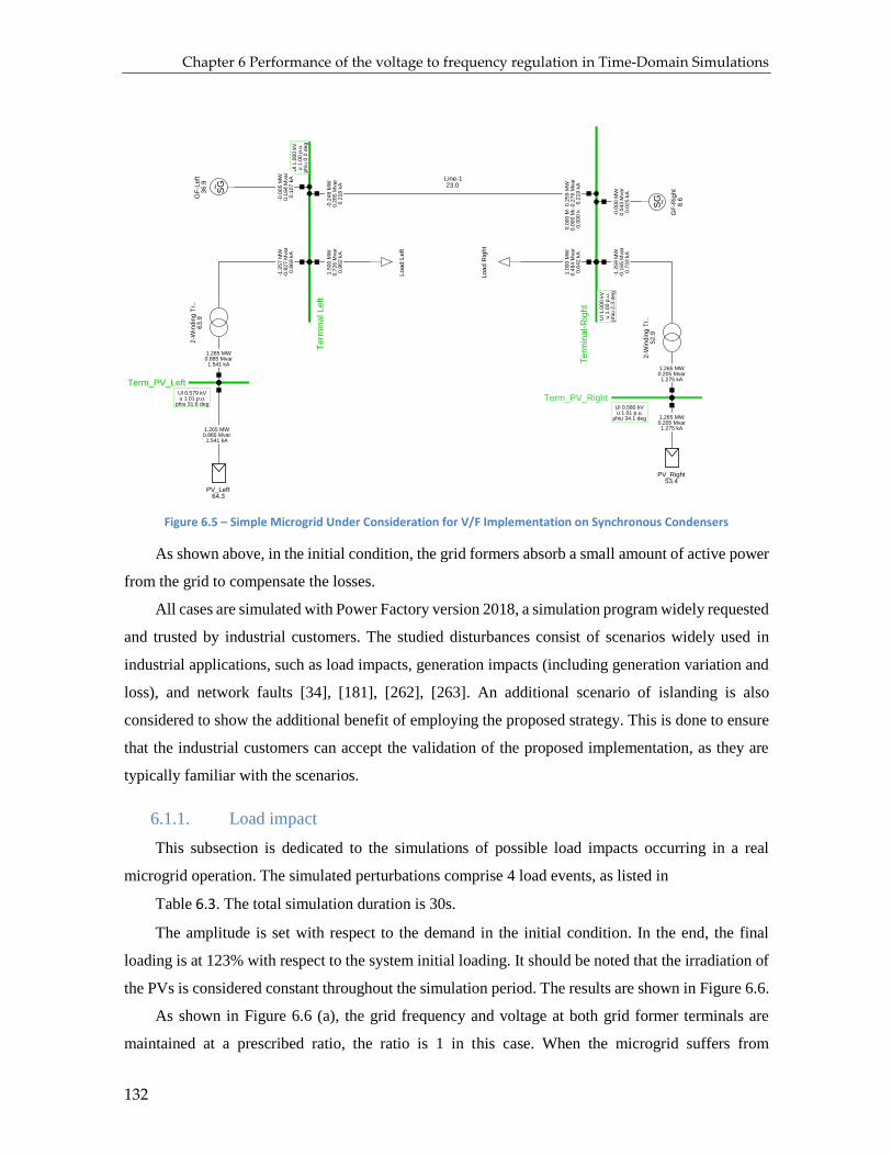
Chapter 6 Performance of the voltage to frequency regulation in Time-Domain Simulations
132
SG ~
SG~
Te
rmin
al-R
igh
t
Ul 1
.00
0 k
Vu
1.0
0 p
.u.
ph
iu 2
.3 d
eg
Term_PV_RightUl 0.580 kVu 1.01 p.u.
phiu 34.1 deg
Term_PV_LeftUl 0.579 kVu 1.01 p.u.
phiu 31.6 deg
Te
rmin
al L
eft
ph
iu 0
.0 d
eg
u 1
.00
p.u
.U
l 1
.00
0 k
V
PV_Right53.4
1.265 MW0.205 Mvar1.275 kA
2-W
ind
ing
Tr.
.5
2.9
-1.2
59
MW
-0.1
65
Mva
r0
.73
3 k
A
1.275 kA0.205 Mvar1.265 MW
0.0
00
kA
0.0
00
Mva
r0.0
00
MW
PV_Left64.3
1.265 MW0.885 Mvar1.541 kA
2-W
ind
ing
Tr.
.6
3.9
0.8
69
kA
-0.8
27
Mva
r-1
.25
7 M
W
1.541 kA0.885 Mvar1.265 MW
GF
-Rig
ht
8.6
-0.0
00
MW
0.0
43
Mva
r0.0
25
kA
Lo
ad
Le
ft
1.5
00
MW
0.7
26
Mva
r0
.96
2 k
A
36
.9G
F-L
eft
0.1
07
kA
0.1
84
Mva
r-0
.00
5 M
W
Lo
ad
Rig
ht
0.6
42
kA
0.4
84
Mva
r1.0
00
MW
23.0Line-1
-0.2
48
MW
0.2
85
Mva
r0
.21
8 k
A
0.2
19
kA
-0.2
76
Mva
r0
.25
9 M
W
Figure 6.5 – Simple Microgrid Under Consideration for V/F Implementation on Synchronous Condensers
As shown above, in the initial condition, the grid formers absorb a small amount of active power
from the grid to compensate the losses.
All cases are simulated with Power Factory version 2018, a simulation program widely requested
and trusted by industrial customers. The studied disturbances consist of scenarios widely used in
industrial applications, such as load impacts, generation impacts (including generation variation and
loss), and network faults [34], [181], [262], [263]. An additional scenario of islanding is also
considered to show the additional benefit of employing the proposed strategy. This is done to ensure
that the industrial customers can accept the validation of the proposed implementation, as they are
typically familiar with the scenarios.
6.1.1. Load impact
This subsection is dedicated to the simulations of possible load impacts occurring in a real
microgrid operation. The simulated perturbations comprise 4 load events, as listed in
Table 6.3. The total simulation duration is 30s.
The amplitude is set with respect to the demand in the initial condition. In the end, the final
loading is at 123% with respect to the system initial loading. It should be noted that the irradiation of
the PVs is considered constant throughout the simulation period. The results are shown in Figure 6.6.
As shown in Figure 6.6 (a), the grid frequency and voltage at both grid former terminals are
maintained at a prescribed ratio, the ratio is 1 in this case. When the microgrid suffers from

Chapter 6 Performance of the voltage to frequency regulation in Time-Domain Simulations
133
underproduction, the frequency naturally drops due to the swing equation, and the V/f regulation
implemented on the voltage regulator will maintain the voltage to frequency ratio. This results in a
decrease in power demand due to the solidary behavior of loads, and the microgrid ends up in a new
stable operating point.
When the system loses a portion of load (for example due to manual action of microgrid operator
or due to voluntary actions of the consumactors), the frequency increases. The system will eventually
find a new stable operation point where the power equilibrium is reached.
In all the cases, the PV is able to maintain its active power production throughout the simulation.
This is in line with the overview of the V/f strategy described in Figure 5.1 where energy producers
possess constant power behavior with respect to voltage and frequency variations. Understandably,
the current has to increase when the voltage drops in order to maintain the same power output. In this
case, the current limit (typically around 1.1 p.u.) is not attained. Otherwise, the active power
production may have to be reduced to satisfy the current limit. However, this is not likely to happen
as the capacity of VRES is still typically designed well above the peak load demand of a system due
to their low capacity factor [174].
Table 6.3 – Simulated Load Impacts
Time Target Impact Amplitude Ramp/Step
Duration
t = 1s Load Left P and Q +10% Step -
t = 2s Load Left P and Q -10% Ramp 2s
t = 5s Load Left P and Q +25% Ramp 2s
t = 8s Load Right P and Q +20% Ramp 2s
30.00023.80017.60011.4005.2000-1.0000 [s]
1.03
0.99
0.95
0.91
0.87
0.83
[p.u.]
GF-Left: Terminal VoltageGF-Right: Terminal Voltage
27.842 s0.851 p.u.
30.00023.80017.60011.4005.2000-1.0000 [s]
1.03
0.99
0.95
0.91
0.87
0.83
[p.u.]
GF-Left: SpeedGF-Right: Speed
27.702 s0.851 p.u.
(a)

Chapter 6 Performance of the voltage to frequency regulation in Time-Domain Simulations
134
30.00023.80017.60011.4005.2000-1.0000 [s]
1.295
1.270
1.245
1.220
1.195
1.170
[MW]
PV_Left: Active PowerPV_Right: Active Power
30.00023.80017.60011.4005.2000-1.0000 [s]
0.75
0.70
0.65
0.60
0.55
0.50
[p.u.]
PV_Left: Positive-Sequence Current, MagnitudePV_Right: Positive-Sequence Current, Magnitude
(b)
30.00023.80017.60011.4005.2000-1.0000 [s]
0.925
0.800
0.675
0.550
0.425
0.300
[Mvar]
Load Left: Total Reactive PowerLoad Right: Total Reactive Power
30.00023.80017.60011.4005.2000-1.0000 [s]
1.80
1.60
1.40
1.20
1.00
0.80
[MW]
Load Left: Total Active PowerLoad Right: Total Active Power
(c)
Figure 6.6 – V/f strategy performance following load impacts, implementation on synchronous condensers (a) measurement at grid formers (b) PV Inverters (c) Loads
6.1.2. Generation Impact
This subsection is dedicated to the simulations of possible generation drops occurring in a real
microgrid operation due to the intermittency of the VRES such as clouds. The simulated perturbations
comprise of 4 events as listed in Table 6.4. The total simulation time is 30 s.
Table 6.4 – Simulated Generation Impacts
Time Target Impact Amplitude Ramp/Step
Duration
t = 1s PV_Left P -30% Ramp 2s
t = 2s PV_Right P -30% Ramp 2s
t = 5s PV_Left P +15% Ramp 5s
t = 6s PV_Right P +15% Ramp 5s
The amplitude shown above is set with respect to the PV active power generation in the initial
condition. In the process, the generation drops to 70% and finally moves to 85% with respect to the
initial generation. The results are shown as follows.

Chapter 6 Performance of the voltage to frequency regulation in Time-Domain Simulations
135
30.00023.80017.60011.4005.2000-1.0000 [s]
1.10
1.00
0.90
0.80
0.70
0.60
[p.u.]
GF-Left: Terminal VoltageGF-Right: Terminal Voltage
25.833 s0.890 p.u.
30.00023.80017.60011.4005.2000-1.0000 [s]
1.20
1.10
1.00
0.90
0.80
0.70
[p.u.]
GF-Left: SpeedGF-Right: Speed
26.633 s0.890 p.u.
(a)
30.00023.80017.60011.4005.2000-1.0000 [s]
1.30
1.20
1.10
1.00
0.90
0.80
[MW]
PV_Left: Active PowerPV_Right: Active Power
30.00023.80017.60011.4005.2000-1.0000 [s]
0.67
0.63
0.59
0.55
0.51
0.47
[p.u.]
PV_Left: Positive-Sequence Current, MagnitudePV_Right: Positive-Sequence Current, Magnitude
(b)
30.00023.80017.60011.4005.2000-1.0000 [s]
0.825
0.700
0.575
0.450
0.325
0.200
[Mvar]
Load Left: Total Reactive PowerLoad Right: Total Reactive Power
30.00023.80017.60011.4005.2000-1.0000 [s]
1.60
1.40
1.20
1.00
0.80
0.60
[MW]
Load Left: Total Active PowerLoad Right: Total Active Power
(c)
Figure 6.7 – V/f strategy performance following generation impacts, implementation on synchronous condensers (a) measurement at grid formers (b) PV Inverters (c) Loads
Again, the grid frequency and voltage at grid former terminals are maintained at a prescribed
ratio, the ratio is 1 in this case. When the microgrid suffers from underproduction, the frequency will
naturally drop, and the V/f regulation implemented on the voltage regulator will maintain the voltage
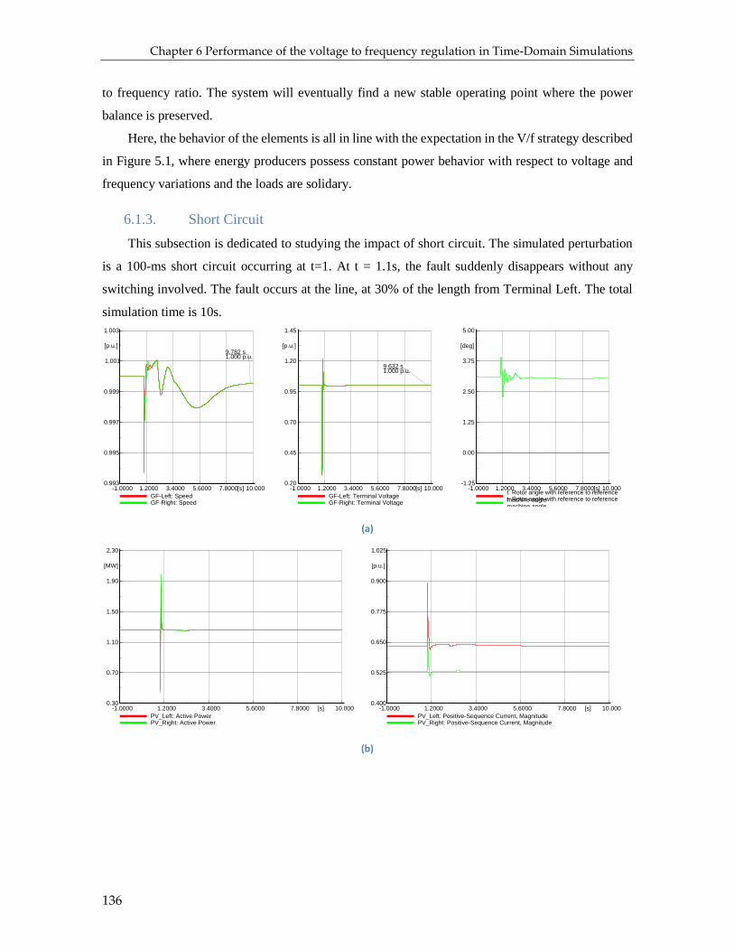
Chapter 6 Performance of the voltage to frequency regulation in Time-Domain Simulations
136
to frequency ratio. The system will eventually find a new stable operating point where the power
balance is preserved.
Here, the behavior of the elements is all in line with the expectation in the V/f strategy described
in Figure 5.1, where energy producers possess constant power behavior with respect to voltage and
frequency variations and the loads are solidary.
6.1.3. Short Circuit
This subsection is dedicated to studying the impact of short circuit. The simulated perturbation
is a 100-ms short circuit occurring at t=1. At t = 1.1s, the fault suddenly disappears without any
switching involved. The fault occurs at the line, at 30% of the length from Terminal Left. The total
simulation time is 10s.
10.0007.80005.60003.40001.2000-1.0000 [s]
1.45
1.20
0.95
0.70
0.45
0.20
[p.u.]
GF-Left: Terminal VoltageGF-Right: Terminal Voltage
9.632 s1.000 p.u.
10.0007.80005.60003.40001.2000-1.0000 [s]
1.003
1.001
0.999
0.997
0.995
0.993
[p.u.]
GF-Left: SpeedGF-Right: Speed
9.782 s1.000 p.u.
10.0007.80005.60003.40001.2000-1.0000 [s]
5.00
3.75
2.50
1.25
0.00
-1.25
[deg]
t: Rotor angle with reference to reference
machine anglet: Rotor angle with reference to reference
machine angle
(a)
10.0007.80005.60003.40001.2000-1.0000 [s]
2.30
1.90
1.50
1.10
0.70
0.30
[MW]
PV_Left: Active PowerPV_Right: Active Power
10.0007.80005.60003.40001.2000-1.0000 [s]
1.025
0.900
0.775
0.650
0.525
0.400
[p.u.]
PV_Left: Positive-Sequence Current, MagnitudePV_Right: Positive-Sequence Current, Magnitude
(b)
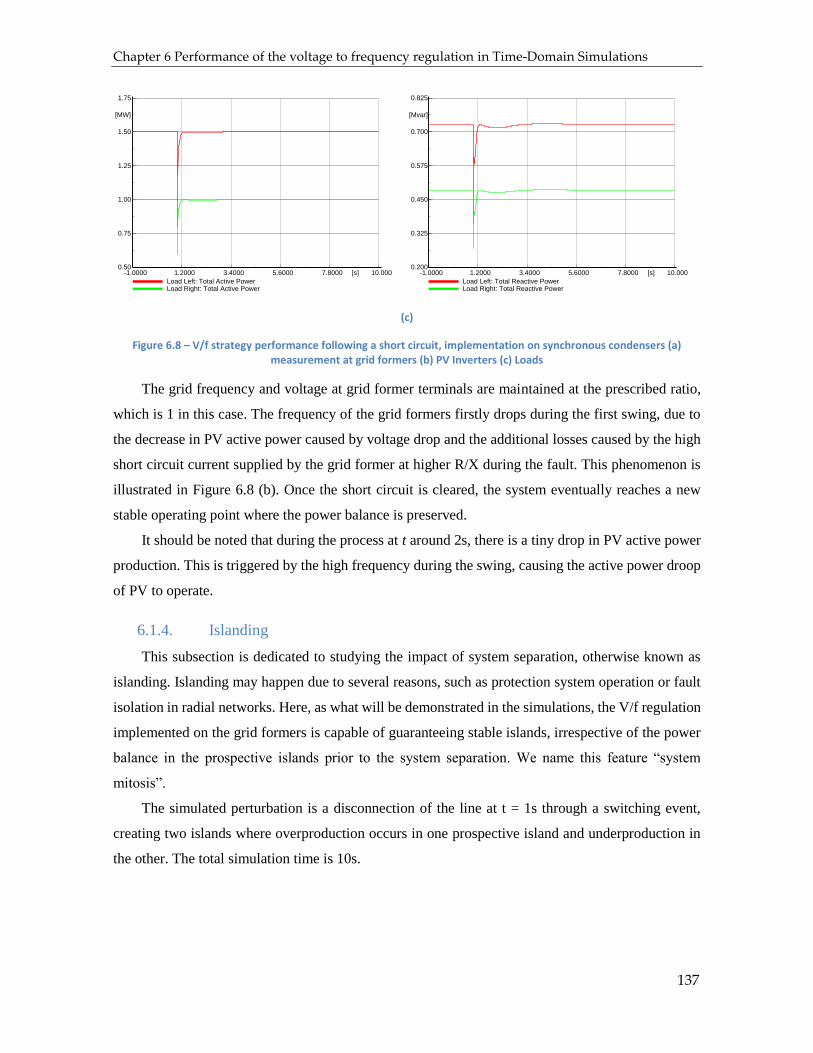
Chapter 6 Performance of the voltage to frequency regulation in Time-Domain Simulations
137
10.0007.80005.60003.40001.2000-1.0000 [s]
0.825
0.700
0.575
0.450
0.325
0.200
[Mvar]
Load Left: Total Reactive PowerLoad Right: Total Reactive Power
10.0007.80005.60003.40001.2000-1.0000 [s]
1.75
1.50
1.25
1.00
0.75
0.50
[MW]
Load Left: Total Active PowerLoad Right: Total Active Power
(c)
Figure 6.8 – V/f strategy performance following a short circuit, implementation on synchronous condensers (a) measurement at grid formers (b) PV Inverters (c) Loads
The grid frequency and voltage at grid former terminals are maintained at the prescribed ratio,
which is 1 in this case. The frequency of the grid formers firstly drops during the first swing, due to
the decrease in PV active power caused by voltage drop and the additional losses caused by the high
short circuit current supplied by the grid former at higher R/X during the fault. This phenomenon is
illustrated in Figure 6.8 (b). Once the short circuit is cleared, the system eventually reaches a new
stable operating point where the power balance is preserved.
It should be noted that during the process at t around 2s, there is a tiny drop in PV active power
production. This is triggered by the high frequency during the swing, causing the active power droop
of PV to operate.
6.1.4. Islanding
This subsection is dedicated to studying the impact of system separation, otherwise known as
islanding. Islanding may happen due to several reasons, such as protection system operation or fault
isolation in radial networks. Here, as what will be demonstrated in the simulations, the V/f regulation
implemented on the grid formers is capable of guaranteeing stable islands, irrespective of the power
balance in the prospective islands prior to the system separation. We name this feature “system
mitosis”.
The simulated perturbation is a disconnection of the line at t = 1s through a switching event,
creating two islands where overproduction occurs in one prospective island and underproduction in
the other. The total simulation time is 10s.

Chapter 6 Performance of the voltage to frequency regulation in Time-Domain Simulations
138
10.0007.80005.60003.40001.2000-1.0000 [s]
1.30
1.20
1.10
1.00
0.90
0.80
[p.u.]
GF-Left: Terminal VoltageGF-Right: Terminal Voltage
9.438 s1.003 p.u.
9.648 s0.877 p.u.
10.0007.80005.60003.40001.2000-1.0000 [s]
1.20
1.10
1.00
0.90
0.80
0.70
[p.u.]
GF-Left: SpeedGF-Right: Speed
9.538 s1.003 p.u.
9.838 s0.878 p.u.
(a)
10.0007.80005.60003.40001.2000-1.0000 [s]
1.525
1.400
1.275
1.150
1.025
0.900
[MW]
PV_Left: Active PowerPV_Right: Active Power
10.0007.80005.60003.40001.2000-1.0000 [s]
0.80
0.70
0.60
0.50
0.40
0.30
[p.u.]
PV_Left: Positive-Sequence Current, MagnitudePV_Right: Positive-Sequence Current, Magnitude
(b)
10.0007.80005.60003.40001.2000-1.0000 [s]
0.925
0.800
0.675
0.550
0.425
0.300
[Mvar]
Load Left: Total Reactive PowerLoad Right: Total Reactive Power
10.0007.80005.60003.40001.2000-1.0000 [s]
1.80
1.60
1.40
1.20
1.00
0.80
[MW]
Load Left: Total Active PowerLoad Right: Total Active Power
(c)
Figure 6.9 – V/f strategy performance following system mitosis, implementation on synchronous condensers (a) measurement at grid formers (b) PV Inverters (c) Loads
Prior to the system splitting, the active power flow is from the system on the right to the system
on the left, as shown in Figure 6.9. Consequently, overproduction is happening in the right subsystem

Chapter 6 Performance of the voltage to frequency regulation in Time-Domain Simulations
139
and underproduction in the left subsystem. After the system is separated into two islands, both islands
can eventually reach a new stable operating point. The system on the right is able to maintain the
operation at nominal operating conditions, where the voltage and frequency are maintained close to
1 per unit. The overproduction naturally increases the frequency of the grid former, which in turn
triggers the active power droop of the PV, causing the active power production to be curtailed. This
is why the final frequency is slightly over 1 per unit.
On the other hand, the system on the left, characterized by underproduction prior to the
separation, experiences higher deviations in voltage and frequency at the new stable operating point,
where the power equilibrium is preserved. Here, the PV is again capable of maintaining the constant
power producing behavior and the loads are solidary to the voltage and frequency variations.
6.2. V/f regulation applied on Grid Forming Inverters
In the following discussions, the V/f strategy is implemented on grid forming converters, which
serve as the grid forming elements. The technical background of the implementation is discussed in
Subchapter 5.2.3. The same models of PV inverters and loads as those in Subchapter 6.1 are
employed. A simple microgrid is used to illustrate the performance of the implementation. The single
line diagram and the initial conditions are shown in Figure 6.10. The following data, unless otherwise
stated, are used in the model:
Table 6.5 – Data and Parameters the simulations with grid forming inverters
Element Data/Parameter Value Unit
Grid Formers (GF-Left, GF-Right)
MVA rating 1 MVA
Nominal Voltage 1 kV
Inertia Constant I 5 s
V/f constant 1 pu/pu
PV Inverter (PV_Left, PV_Right)
MVA Rating 2.4 MVA
MWp Rating 2 MWp
Nominal Voltage 0.575 kV
Transformer
MVA Rating 2.4 MVA
Primary Voltage 0.575 kV
Secondary Voltage 1 kV
Line
Length 1 km
Resistance per km 0.08 Ω
Reactance per km 0.08 Ω
Contrary to synchronous condensers, important parameters of grid forming inverters, such as
inertia constant, can be changed at any moment as they are not physical quantities anymore. There is
no physical relation between the amount of power absorbed/released and the rate of change of

Chapter 6 Performance of the voltage to frequency regulation in Time-Domain Simulations
140
frequency. Although the swing equation is implemented in the control systems of the grid forming
converters, the out-of-step phenomenon can always be avoided, as sudden frequency change and
phase jumps are possible when the appropriate control strategies are in place.
In the simulations, two sets of load coefficients are investigated. They are shown as follows. The
first load represents a typical residential-commercial load (provided by Schneider Electric), while the
other one represents a standard impedance load. It should be noted that the residential-commercial
load has a considerable level of constant power.
Table 6.6 – Load proportion and coefficients for the simulations
Load p1 p2 p3 q1 q2 q3 Kpf
Residential- commercial Load
0.76 -0.52 0.76 5.83 -11.75 6.92 0.5
Impedance Load 0 0 1 0 0 1 0
Term_PV_Left..0.576 kV1.002 p.u.
30.817 deg
Term_PV_Left0.572 kV0.995 p.u.
29.594 deg
Term_Right1.000 kV1.000 p.u.-0.251 d..
Term_Left1.000 kV1.000 p.u.-1.399 d..
PV_Left(1)31.5
0.755 MW-0.000 Mvar
0.756 kA1.000
2-W
ind
ing
Tr.
.3
1.4
-0.753 MW0.014 Mvar0.435 kA-1.000
1.0000.756 kA
-0.000 Mvar0.755 MW
PV_Left38.0
0.755 MW0.512 Mvar0.920 kA0.828
2-W
ind
ing
Tr.
.3
8.2
-0.752 MW-0.491 Mvar
0.519 kA-0.837
0.8280.920 kA
0.512 Mvar0.755 MW
Load Right
0.9000.641 kA0.484 M..1.000 MW
0.7140.205 kA-0.248 M..
0.253 ..
Line_121.5
-0.7010.204 kA
0.253 Mvar-0.248 MW
Load Left
0.9000.962 kA
0.726 Mvar1.500 MW
0.6990.403 kA
0.512 Mvar0.500 MW
Grid Former LeftGrid Former Right
0.8830.323 kA
0.266 Mvar0.500 MW
Figure 6.10 – Simple Microgrid under Consideration for V/F Implementation on Grid Forming Converters
Again, all cases are simulated with Power Factory version 2018, a simulation program widely
trusted by industrial customers. The studied disturbances consist of scenarios widely used in industrial
applications.
6.2.1. Load impact
This subsection is dedicated to the simulations of possible load impacts occurring in a real
microgrid operation. The simulated perturbations comprise 4 load events, as listed in Table 6.7. The
total simulation duration is 30s.
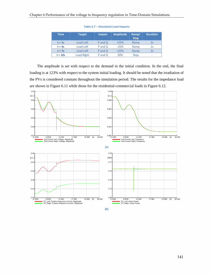
Chapter 6 Performance of the voltage to frequency regulation in Time-Domain Simulations
141
Table 6.7 – Simulated Load Impacts
Time Target Impact Amplitude Ramp/Step
Duration
t = 1s Load Left P and Q +25% Ramp 2s
t = 4s Load Left P and Q -25% Ramp 2s
t = 7s Load Left P and Q +25% Ramp 2s
t = 10s Load Right P and Q 20% Step -
The amplitude is set with respect to the demand in the initial condition. In the end, the final
loading is at 123% with respect to the system initial loading. It should be noted that the irradiation of
the PVs is considered constant throughout the simulation period. The results for the impedance load
are shown in Figure 6.11 while those for the residential-commercial loads in Figure 6.12.
30.00023.98017.96011.9405.9200-0.1000 [s]
1.02
0.99
0.96
0.93
0.90
0.87
[p.u.]
Grid Former Left: Voltage, MagnitudeGrid Former Right: Voltage, Magnitude
30.00023.98017.96011.9405.9200-0.1000 [s]
1.015
0.990
0.965
0.940
0.915
0.890
[p.u.]
Grid Former Left: FrequencyGrid Former Right: Frequency
(a)
30.00023.98017.96011.9405.9200-0.1000 [s]
0.45
0.42
0.39
0.36
0.33
0.30
[p.u.]
PV_Left: Positive-Sequence Current, MagnitudePV_Right: Positive-Sequence Current, Magnitude
30.00023.98017.96011.9405.9200-0.1000 [s]
0.79
0.77
0.75
0.73
0.71
0.69
[MW]
PV_Left: Active PowerPV_Right: Active Power
(b)

Chapter 6 Performance of the voltage to frequency regulation in Time-Domain Simulations
142
30.00023.98017.96011.9405.9200-0.1000 [s]
0.90
0.80
0.70
0.60
0.50
0.40
[Mvar]
Load Left: Reactive PowerLoad Right: Reactive Power
30.00023.98017.96011.9405.9200-0.1000 [s]
1.80
1.60
1.40
1.20
1.00
0.80
[MW]
Load Left: Active PowerLoad Right: Active Power
(c)
Figure 6.11 – V/f strategy performance following load impacts, implementation on grid forming converters, impedance load (a) measurement at grid formers (b) PV Inverters (c) Loads
When the loads are of impedance-type, the grid forming converters are capable of varying the
frequency and voltage in such a way in transient state, that the V/f ratio is maintained and the
microgrid reaches a new state where the power equilibrium is preserved, thanks to the solidary loads.
However, this is not always the case. As shown in the following curves, when the residential-
commercial load type is considered in the simulation, the load contains high constant-power share
which will cause the transient state to become more demanding. The current may soar when the
voltage drops. As the grid forming inverters are characterized by strict current limits, this may cause
the microgrid to fail to survive the transient period due to the inability to recover the voltage.
30.00023.98017.96011.9405.9200-0.1000 [s]
1.20
0.90
0.60
0.30
0.00
-0.30
[p.u.]
30.00023.98017.96011.9405.9200-0.1000 [s]
3.30
2.80
2.30
1.80
1.30
0.80
[p.u.]
Grid Forming Left: FrequencyGrid Forming Right: Frequency
30.00023.98017.96011.9405.9200-0.1000 [s]
1.30
1.10
0.90
0.70
0.50
0.30
[p.u.]
Grid Former Left: Output Current, MagnitudeGrid Former Right: Output Current, Magnitude
Grid Former Left: Voltage, MagnitudeGrid Former Right: Voltage, Magnitude
(a)

Chapter 6 Performance of the voltage to frequency regulation in Time-Domain Simulations
143
30.00023.98017.96011.9405.9200-0.1000 [s]
1.35
1.10
0.85
0.60
0.35
0.10
[p.u.]
PV_Left: Positive-Sequence Current, MagnitudePV_Right: Positive-Sequence Current, Magnitude
30.00023.98017.96011.9405.9200-0.1000 [s]
1.00
0.75
0.50
0.25
0.00
-0.25
[MW]
PV_Left: Active PowerPV_Right: Active Power
(b)
30.00023.98017.96011.9405.9200-0.1000 [s]
1.00
0.80
0.60
0.40
0.20
0.00
[Mvar]
Load Left: Reactive PowerLoad Right: Reactive Power
30.00023.98017.96011.9405.9200-0.1000 [s]
2.00
1.50
1.00
0.50
0.00
-0.50
[MW]
Load Left: Active PowerLoad Right: Active Power
(c)
Figure 6.12 – V/f strategy performance following load impacts, implementation on grid forming converters, residential-commercial loads (a) measurement at grid formers (b) PV Inverters (c) Load
As shown in Figure 6.12 for scenarios where residential-commercial-type loads are studied, the
grid frequency and voltage at grid former terminals are maintained at a prescribed ratio for all ramp
load impacts. However, for the last step load impact at t = 10s, the transient period is very demanding,
as the load demands high current during this period. As the grid forming elements have attained the
current limits, as shown in Figure 6.12 (a), the terminal voltage drops and the voltage recovery cannot
be accomplished, leaving the system to go into a blackout.
6.2.2. Generation Impact
This part is dedicated to the simulations of possible generation drops occurring in a real
microgrid operation due to the intermittency of the VRES. The simulated perturbations comprise of
4 events as listed in
Table 6.8. The total simulation time is 30 s.

Chapter 6 Performance of the voltage to frequency regulation in Time-Domain Simulations
144
Table 6.8 – Simulated Generation Impacts
Time Target Impact Amplitude Ramp/Step
Duration
t = 1s PV_Left P -30% Ramp 2s
t = 2s PV_Right P -30% Ramp 2s
t = 5s PV_Left P +15% Ramp 5s
t = 6s PV_Right P +15% Ramp 5s
The amplitude shown above is set with respect to the PV active power generation in the initial
condition. In the process, the total system generation, comprising of generation from grid forming
inverters and the PVs, drops to 82% and finally settles down at 91% with respect to the total initial
generation. The results for the impedance load are shown in Figure 6.13 while those for the
residential-commercial loads in Figure 6.14.
30.00023.98017.96011.9405.9200-0.1000 [s]
1.04
1.00
0.96
0.92
0.88
0.84
[p.u.]
30.00023.98017.96011.9405.9200-0.1000 [s]
1.04
1.00
0.96
0.92
0.88
0.84
[p.u.]
Grid Former Left: Voltage, MagnitudeGrid Former Right: Voltage, Magnitude
Grid Former Left: FrequencyGrid Former Right: Frequency
(a)
30.00023.98017.96011.9405.9200-0.1000 [s]
0.41
0.37
0.33
0.29
0.25
0.21
[p.u.]
PV_Left: Positive-Sequence Current, MagnitudePV_Right: Positive-Sequence Current, Magnitude
30.00023.98017.96011.9405.9200-0.1000 [s]
0.90
0.80
0.70
0.60
0.50
0.40
[MW]
PV_Left: Active PowerPV_Right: Active Power
(b)

Chapter 6 Performance of the voltage to frequency regulation in Time-Domain Simulations
145
30.00023.98017.96011.9405.9200-0.1000 [s]
0.90
0.80
0.70
0.60
0.50
0.40
[Mvar]
Load Left: Reactive PowerLoad Right: Reactive Power
30.00023.98017.96011.9405.9200-0.1000 [s]
1.70
1.50
1.30
1.10
0.90
0.70
[MW]
Load Left: Active PowerLoad Right: Active Power
(c)
Figure 6.13 – V/f strategy performance following generation impacts, implementation on grid forming converters, impedance load (a) measurement at grid formers (b) PV Inverters (c) Loads
Again, when the loads are of impedance-type, the grid forming converters are capable of varying
the frequency and voltage in such a way in transient state the grid frequency and voltage at grid former
terminals are maintained at the prescribed ratio. When the microgrid suffers from underproduction,
the frequency will drop due to the swing equation which is integrated in the control strategy, and the
V/f regulation will maintain the voltage to frequency ratio. The system will eventually find a new
stable operating point where the power balance is preserved. The problems with regard to current
limits of converters are not found.
When the residential-commercial load type is considered in the simulation, the transient state
due to the simulated perturbations becomes more demanding. The current soars when the voltage
drops. As shown in Figure 6.14 (a), the grid forming inverters are strictly limited in current (as
opposed to synchronous machine technology), which causes the microgrid to fail to survive the
voltage recovery period.
30.00023.98017.96011.9405.9200-0.1000 [s]
1.20
0.90
0.60
0.30
0.00
-0.30
[p.u.]
30.00023.98017.96011.9405.9200-0.1000 [s]
2.70
2.30
1.90
1.50
1.10
0.70
[p.u.]
30.00023.98017.96011.9405.9200-0.1000 [s]
1.40
1.20
1.00
0.80
0.60
0.40
[p.u.]
Grid Forming Left: FrequencyGrid Forming Right: Frequency
Grid Former Left: Output Current, MagnitudeGrid Former Right: Output Current, Magnitude
Grid Former Left: Voltage, MagnitudeGrid Former Right: Voltage, Magnitude
(a)

Chapter 6 Performance of the voltage to frequency regulation in Time-Domain Simulations
146
30.00023.98017.96011.9405.9200-0.1000 [s]
1.20
1.00
0.80
0.60
0.40
0.20
[p.u.]
PV_Left: Positive-Sequence Current, MagnitudePV_Right: Positive-Sequence Current, Magnitude
30.00023.98017.96011.9405.9200-0.1000 [s]
2.00
1.50
1.00
0.50
0.00
-0.50
[MW]
PV_Left: Active PowerPV_Right: Active Power
(b)
30.00023.98017.96011.9405.9200-0.1000 [s]
1.60
1.20
0.80
0.40
0.00
-0.40
[Mvar]
Load Left: Reactive Power
Load Right: Reactive Power
30.00023.98017.96011.9405.9200-0.1000 [s]
1.60
1.20
0.80
0.40
0.00
-0.40
[MW]
Load Left: Active Power
Load Right: Active Power
(c)
Figure 6.14 – V/f strategy performance following generation impacts, implementation on grid forming converters, residential-commercial load (a) measurement at grid formers (b) PV Inverters (c) Loads
6.2.3. Short Circuit
This subsection is dedicated to studying the impact of short circuit. The simulated perturbation
is a 100-ms low impedance short circuit occurring at t=1. At t = 1.1s, the fault suddenly disappears
without any switching involved. The fault occurs at the line, 30% the length from bus Term_Left.
30.00023.98017.96011.9405.9200-0.1000 [s]
1.50
1.30
1.10
0.90
0.70
0.50
[p.u.]
30.00023.98017.96011.9405.9200-0.1000 [s]
1.004
1.000
0.996
0.992
0.988
0.984
[p.u.]
30.00023.98017.96011.9405.9200-0.1000 [s]
1.40
1.20
1.00
0.80
0.60
0.40
[p.u.]
Grid Former Left: Output Current, MagnitudeGrid Former Right: Output Current, Magnitude
1.091 s1.099 p.u.
Grid Former Left: Voltage, MagnitudeGrid Former Right: Voltage, Magnitude
Grid Former Left: FrequencyGrid Former Right: Frequency
(a)

Chapter 6 Performance of the voltage to frequency regulation in Time-Domain Simulations
147
30.00023.98017.96011.9405.9200-0.1000 [s]
1.20
0.90
0.60
0.30
0.00
-0.30
[p.u.]
PV_Left: Positive-Sequence Current, MagnitudePV_Right: Positive-Sequence Current, Magnitude
30.00023.98017.96011.9405.9200-0.1000 [s]
4.00
3.00
2.00
1.00
0.00
-1.00
[MW]
PV_Left: Active PowerPV_Right: Active Power
(b)
30.00023.98017.96011.9405.9200-0.1000 [s]
1.35
1.10
0.85
0.60
0.35
0.10
[Mvar]
Load Left: Reactive PowerLoad Right: Reactive Power
30.00023.98017.96011.9405.9200-0.1000 [s]
2.80
2.30
1.80
1.30
0.80
0.30
[MW]
Load Left: Active PowerLoad Right: Active Power
(c)
Figure 6.15 – V/f strategy performance following a short circuit, implementation on grid forming converters, impedance load (a) measurement at grid formers (b) PV Inverters (c) Loads
During the fault, slight deviations in frequency occur. The grid formers try to maintain the
voltage-to-frequency ratio at the terminal by injecting more current. In the process, the grid forming
converters eventually reach the current saturation limit (at 1.1 per unit), causing the voltage terminal
voltage to drop. After the fault disappears, the power system survives the transition to regain a stable
steady state at the prescribed voltage to frequency ratio. It should be noted that impedance-type loads
are considered in the results shown in Figure 6.15.
In Figure 6.16, an identical short circuit event is simulated, but with residential-commercial-type
loads under consideration. During the short-circuit, the frequency deviates according to the swing
equation implemented in the controls. As what happens in the previous case with the impedance-type
loads, the V/f regulation tries to maintain the voltage to frequency ratio by injecting more current.
Eventually, the grid forming converters reach the saturation limit in current at 1.1 per unit. However,
in this case the system fails to regain the stability after the short circuit is removed. This is due to the
inability of the grid formers to recover the voltage. During the transient state after the fault is removed,
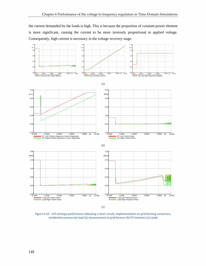
Chapter 6 Performance of the voltage to frequency regulation in Time-Domain Simulations
148
the current demanded by the loads is high. This is because the proportion of constant-power element
is more significant, causing the current to be more inversely proportional to applied voltage.
Consequently, high current is necessary in the voltage recovery stage.
10.0007.98005.96003.94001.9200-0.1000 [s]
1.20
0.90
0.60
0.30
0.00
-0.30
[p.u.]
10.0007.98005.96003.94001.9200-0.1000 [s]
1.90
1.70
1.50
1.30
1.10
0.90
[p.u.]
10.0007.98005.96003.94001.9200-0.1000 [s]
1.40
1.20
1.00
0.80
0.60
0.40
[p.u.]
Grid Former Left: Output Current, MagnitudeGrid Former Right: Output Current, Magnitude
Grid Former Left: Voltage, MagnitudeGrid Former Right: Voltage, Magnitude
Grid Former Left: FrequencyGrid Former Right: Frequency
(a)
10.0007.98005.96003.94001.9200-0.1000 [s]
1.20
0.90
0.60
0.30
0.00
-0.30
[p.u.]
PV_Left: Positive-Sequence Current, MagnitudePV_Right: Positive-Sequence Current, Magnitude
10.0007.98005.96003.94001.9200-0.1000 [s]
4.00
3.00
2.00
1.00
0.00
-1.00
[MW]
PV_Left: Active PowerPV_Right: Active Power
(b)
10.0007.98005.96003.94001.9200-0.1000 [s]
1.00
0.75
0.50
0.25
0.00
-0.25
[Mvar]
Load Left: Reactive PowerLoad Right: Reactive Power
10.0007.98005.96003.94001.9200-0.1000 [s]
2.00
1.50
1.00
0.50
0.00
-0.50
[MW]
Load Left: Active PowerLoad Right: Active Power
(c)
Figure 6.16 – V/f strategy performance following a short circuit, implementation on grid forming converters, residential-commercial load (a) measurement at grid formers (b) PV Inverters (c) Loads

Chapter 6 Performance of the voltage to frequency regulation in Time-Domain Simulations
149
6.2.4. Islanding
This subsection is dedicated to studying the impact of the system separation, otherwise known
as islanding. Typically, the V/f strategy is capable of guaranteeing stable islands, irrespective of the
power balance in the prospective islands prior to the system separation. As a reminder, this feature is
what we call “system mitosis”.
The simulated perturbation is a disconnection of the line at t = 1s through a switching event,
creating two islands where overproduction occurs in one prospective island and underproduction in
the other. The total simulation time is 30s. The simulations results considering the impedance-type
loads are shown in Figure 6.17 while the residential-commercial-type loads in Figure 6.18.
30.00023.98017.96011.9405.9200-0.1000 [s]
1.20
1.10
1.00
0.90
0.80
0.70
[p.u.]
26.319 s0.913 p.u.
30.00023.98017.96011.9405.9200-0.1000 [s]
1.025
1.000
0.975
0.950
0.925
0.900
[p.u.]
27.684 s0.913 p.u.
Grid Former Left: Voltage, MagnitudeGrid Former Right: Voltage, Magnitude
Grid Former Left: FrequencyGrid Former Right: Frequency
(a)
30.00023.98017.96011.9405.9200-0.1000 [s]
1.20
0.90
0.60
0.30
0.00
-0.30
[p.u.]
PV_Left: Positive-Sequence Current, MagnitudePV_Right: Positive-Sequence Current, Magnitude
30.00023.98017.96011.9405.9200-0.1000 [s]
4.00
3.00
2.00
1.00
0.00
-1.00
[MW]
PV_Left: Active PowerPV_Right: Active Power
(b)

Chapter 6 Performance of the voltage to frequency regulation in Time-Domain Simulations
150
30.00023.98017.96011.9405.9200-0.1000 [s]
1.35
1.10
0.85
0.60
0.35
0.10
[Mvar]
Load Left: Reactive PowerLoad Right: Reactive Power
30.00023.98017.96011.9405.9200-0.1000 [s]
2.80
2.30
1.80
1.30
0.80
0.30
[MW]
Load Left: Active PowerLoad Right: Active Power
(c)
Figure 6.17 – V/f strategy performance following system mitosis, implementation on grid forming converters, impedance load (a) measurement at grid formers (b) PV Inverters (c) Loads
Prior to the system splitting, the active power flow is from the system on the right to the system
on the left, as shown in Figure 6.10. Consequently, the overproduction is happening in the right
subsystem and the underproduction in the left subsystem.
Once the system is separated into two islands, both islands can eventually reach a new stable
operating point for the cases considering the impedance-type loads. The system on the right is able to
maintain the operation at nominal operating conditions, where the voltage and frequency are
maintained close to 1 per unit. The overproduction increases the frequency of the grid former due to
the implemented swing equation in the controls, which activates the active power droop of the PV,
causing the active power production to be curtailed. This is why the final frequency is slightly over 1
per unit. On the other hand, the underproducing system on the left experiences higher deviations in
voltage and frequency at the new stable operating point, where the power equilibrium is preserved
thanks to the solidary characteristics of the loads. Here, the PV is again capable of maintaining the
constant power behavior.
However, when the residential-commercial type loads are studied, different results are obtained.
The proportion of constant-power element in the load model is higher which causes difficulties in the
transitory phase following the system splitting. As the grid forming converters are strictly limited in
current, both new microgrids are not able to survive the transition and end up in the blackout.

Chapter 6 Performance of the voltage to frequency regulation in Time-Domain Simulations
151
10.0007.98005.96003.94001.9200-0.1000 [s]
1.60
1.20
0.80
0.40
0.00
-0.40
[p.u.]
10.0007.98005.96003.94001.9200-0.1000 [s]
1.90
1.70
1.50
1.30
1.10
0.90
[p.u.]
10.0007.98005.96003.94001.9200-0.1000 [s]
1.20
0.90
0.60
0.30
0.00
-0.30
[p.u.]
Grid Former Left: Output Current, MagnitudeGrid Former Right: Output Current, Magnitude
Grid Former Left: Voltage, MagnitudeGrid Former Right: Voltage, Magnitude
Grid Former Left: FrequencyGrid Former Right: Frequency
(a)
10.0007.98005.96003.94001.9200-0.1000 [s]
1.25
1.00
0.75
0.50
0.25
0.00
[p.u.]
PV_Left: Positive-Sequence Current, MagnitudePV_Right: Positive-Sequence Current, Magnitude
10.0007.98005.96003.94001.9200-0.1000 [s]
1.00
0.75
0.50
0.25
0.00
-0.25
[MW]
PV_Left: Active PowerPV_Right: Active Power
(b)
10.0007.98005.96003.94001.9200-0.1000 [s]
1.00
0.75
0.50
0.25
0.00
-0.25
[Mvar]
Load Left: Reactive PowerLoad Right: Reactive Power
10.0007.98005.96003.94001.9200-0.1000 [s]
1.60
1.20
0.80
0.40
0.00
-0.40
[MW]
Load Left: Active PowerLoad Right: Active Power
(c)
Figure 6.18 – V/f strategy performance following system mitosis, implementation on grid forming converters, residential-commercial load (a) measurement at grid formers (b) PV Inverters (c) Loads
6.2.5. Comment on the voltage recovery problem
When the microgrid contains a considerable portion of constant power loads, voltage recovery
period is very demanding for grid forming converters. This particular type of load is very onerous
during voltage excursions as the demanded current is inversely proportional to the applied voltage.

Chapter 6 Performance of the voltage to frequency regulation in Time-Domain Simulations
152
As shown in the Figures in Subchapter Figure 6.2, the grid forming converters deliver the expected
performance when the loads are not demanding, i.e. the impedance-type loads. However, when the
loads comprise of high proportions of constant power element, the grid forming inverters may
struggle during the transitory period, as they are limited by a strict current limit which may cause a
failure at recovering the voltage. It should be noted that this particular problem is not observed for
the implementation on synchronous condensers. Consequently, the type of load need to be taken into
account when selecting the grid former technology, or supplementary strategies may need to be
developed if an inverter, which is strictly limited in current by design, is chosen as the grid forming
element. Otherwise, oversizing may be a potential solution, but it may outweigh the benefits of
employing static converters in the first place.
6.3. Comparison with the Present Grid Forming Solutions This subchapter is dedicated to the comparison of several grid forming solutions, namely the
V/f-implemented grid formers, the VSG, and the UPS. The main distinguishing point is that the grid
formers in the V/f strategy are not required to produce energy in the steady state, contrary to the other
grid forming solutions.
A comparison on the control strategy, the sizing, and the system design is summarized in the
following table.
Table 6.9 – Comparison of the current grid forming solutions
Solution System regulation MVA Sizing Multi grid formers currently possible?
Diesel Genset Classical regulations
(droop, AVR) Peak load Yes
UPS Isosynchronous,
AVR 3 times the
excepted peak load No
VSG classical regulations
(droop, AVR) 1.1-1.2 times the
peak load Yes
V/f-implemented grid formers
V/f strategy Around 25% of
system peak load Yes
It should also be noted that only diesel generators produce the electrical energy on their own,
while UPS and VSG are basically a storage element. Currently, the operation of multiple UPS without
a centralized controller is not yet mature. In its implementation, the UPS is also typically oversized
compared to the loads it supplies. When V/f-implemented grid formers are in place, only small energy
storage is necessary to support the grid during the transient state. On the other hand, VSG and UPS
require larger energy storage to function. The effectivity of the UPS and VSG is entirely dependent
on the stored energy in the storage element. Once the stored energy runs out, the impact to the grid is
equivalent to that of generator loss.
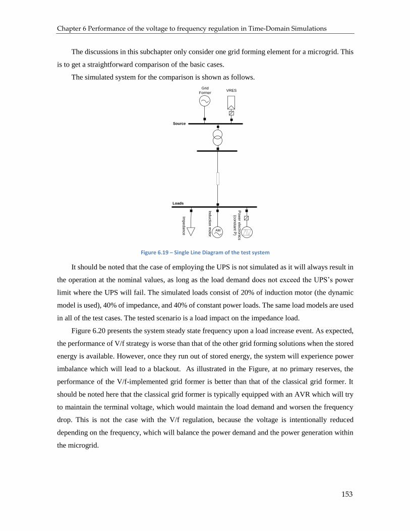
Chapter 6 Performance of the voltage to frequency regulation in Time-Domain Simulations
153
The discussions in this subchapter only consider one grid forming element for a microgrid. This
is to get a straightforward comparison of the basic cases.
The simulated system for the comparison is shown as follows.
AM
Source
Loads
Grid
FormerVRES
Imp
ed
an
ce
Ind
uctio
n m
oto
r
Po
we
r ele
ctro
nic
s
(co
nsta
nt P
)
Figure 6.19 – Single Line Diagram of the test system
It should be noted that the case of employing the UPS is not simulated as it will always result in
the operation at the nominal values, as long as the load demand does not exceed the UPS’s power
limit where the UPS will fail. The simulated loads consist of 20% of induction motor (the dynamic
model is used), 40% of impedance, and 40% of constant power loads. The same load models are used
in all of the test cases. The tested scenario is a load impact on the impedance load.
Figure 6.20 presents the system steady state frequency upon a load increase event. As expected,
the performance of V/f strategy is worse than that of the other grid forming solutions when the stored
energy is available. However, once they run out of stored energy, the system will experience power
imbalance which will lead to a blackout. As illustrated in the Figure, at no primary reserves, the
performance of the V/f-implemented grid former is better than that of the classical grid former. It
should be noted here that the classical grid former is typically equipped with an AVR which will try
to maintain the terminal voltage, which would maintain the load demand and worsen the frequency
drop. This is not the case with the V/f regulation, because the voltage is intentionally reduced
depending on the frequency, which will balance the power demand and the power generation within
the microgrid.
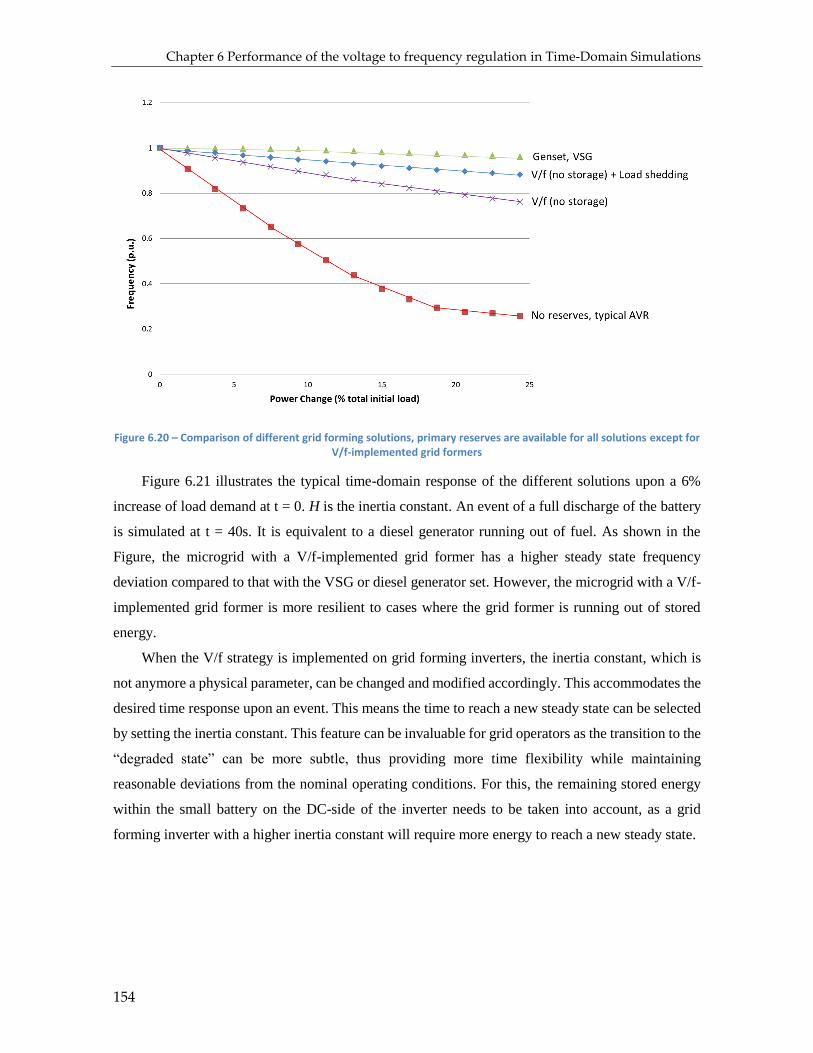
Chapter 6 Performance of the voltage to frequency regulation in Time-Domain Simulations
154
Figure 6.20 – Comparison of different grid forming solutions, primary reserves are available for all solutions except for V/f-implemented grid formers
Figure 6.21 illustrates the typical time-domain response of the different solutions upon a 6%
increase of load demand at t = 0. H is the inertia constant. An event of a full discharge of the battery
is simulated at t = 40s. It is equivalent to a diesel generator running out of fuel. As shown in the
Figure, the microgrid with a V/f-implemented grid former has a higher steady state frequency
deviation compared to that with the VSG or diesel generator set. However, the microgrid with a V/f-
implemented grid former is more resilient to cases where the grid former is running out of stored
energy.
When the V/f strategy is implemented on grid forming inverters, the inertia constant, which is
not anymore a physical parameter, can be changed and modified accordingly. This accommodates the
desired time response upon an event. This means the time to reach a new steady state can be selected
by setting the inertia constant. This feature can be invaluable for grid operators as the transition to the
“degraded state” can be more subtle, thus providing more time flexibility while maintaining
reasonable deviations from the nominal operating conditions. For this, the remaining stored energy
within the small battery on the DC-side of the inverter needs to be taken into account, as a grid
forming inverter with a higher inertia constant will require more energy to reach a new steady state.
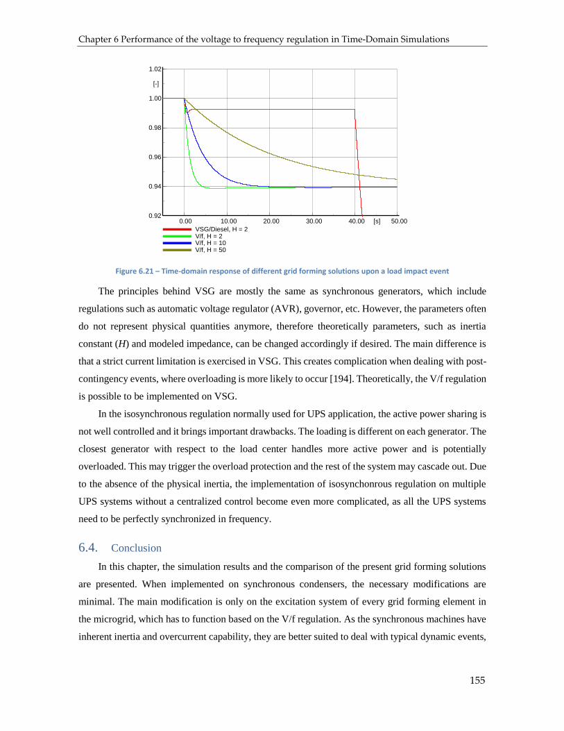
Chapter 6 Performance of the voltage to frequency regulation in Time-Domain Simulations
155
50.0040.0030.0020.0010.000.00 [s]
1.02
1.00
0.98
0.96
0.94
0.92
[-]
VSG/Diesel, H = 2V/f, H = 2V/f, H = 10V/f, H = 50
Figure 6.21 – Time-domain response of different grid forming solutions upon a load impact event
The principles behind VSG are mostly the same as synchronous generators, which include
regulations such as automatic voltage regulator (AVR), governor, etc. However, the parameters often
do not represent physical quantities anymore, therefore theoretically parameters, such as inertia
constant (H) and modeled impedance, can be changed accordingly if desired. The main difference is
that a strict current limitation is exercised in VSG. This creates complication when dealing with post-
contingency events, where overloading is more likely to occur [194]. Theoretically, the V/f regulation
is possible to be implemented on VSG.
In the isosynchronous regulation normally used for UPS application, the active power sharing is
not well controlled and it brings important drawbacks. The loading is different on each generator. The
closest generator with respect to the load center handles more active power and is potentially
overloaded. This may trigger the overload protection and the rest of the system may cascade out. Due
to the absence of the physical inertia, the implementation of isosynchonrous regulation on multiple
UPS systems without a centralized control become even more complicated, as all the UPS systems
need to be perfectly synchronized in frequency.
6.4. Conclusion
In this chapter, the simulation results and the comparison of the present grid forming solutions
are presented. When implemented on synchronous condensers, the necessary modifications are
minimal. The main modification is only on the excitation system of every grid forming element in
the microgrid, which has to function based on the V/f regulation. As the synchronous machines have
inherent inertia and overcurrent capability, they are better suited to deal with typical dynamic events,

Chapter 6 Performance of the voltage to frequency regulation in Time-Domain Simulations
156
which often include power inequilibrium problems and voltage recovery problems. In contrast, the
inverter-based grid formers have difficulty in dealing with voltage recovery or step transition, because
they are limited by current saturation. However, such problems arise from the design approach of
inverters, and not from the V/f strategy.

157
Chapter 7 Validation of the voltage to frequency
regulation through Real-time HIL Simulations
This chapter addresses the performance of the proposed voltage-to-frequency regulation
implemented on a synchronous condenser through the experimentation in real-time hardware-in-the-
loop platform based on RT-Lab. A simple test system comprised of a number of simulated and
physical elements has been constructed for this purpose. Several scenarios are taken into account to
understand the behavior of the system following typical perturbations that may occur in microgrid
operations.
7.1. Introduction to Hardware in-the-loop Real-Time Simulation
Digital real-time simulation (DRTS) of an electric power system provides an accurate
reproduction of the output waveforms (voltage and current), useful for representing the real power
system being modeled [264]. It solves the model equations within the same time in real-world clock,
although the output is in discrete time intervals due to the use of time-step.
Hardware in the loop (HIL) is one of two categories of DRTS, the other one being fully digital
real-time simulation. It refers to the condition where certain parts of the digital simulation include
real physical components. The physical components are connected via input-output interfaces, such
as digital-to-analog or analog-to-digital converters and filters. HIL is used for prototyping. For power-
hardware-in-the-loop (PHIL) applications, amplifiers are necessary for reproducing the actual signals
(e.g. current, voltage) and supplying the power exchange to the physical elements. A real-time
simulator’s time step is typically around 50 μs or smaller, which is considered suitable for a dynamic
study in 50/60 Hz power systems.
OPAL RT
RT LAB is a brand of digital real-time simulator capable of performing HIL simulations
developed and marketed by OPAL RT Technology, a Canada-based company. Modeling can be
carried out in Matlab’s Simulink and this product is compatible with Simulink solvers. Real time HIL
simulations with OPAL RT are suitable for studies on power electronics, power systems, and control
systems.
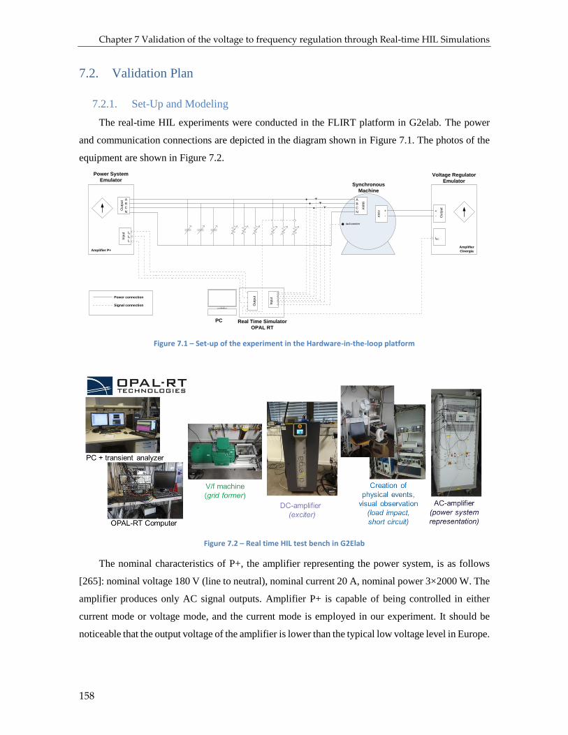
Chapter 7 Validation of the voltage to frequency regulation through Real-time HIL Simulations
158
7.2. Validation Plan
7.2.1. Set-Up and Modeling
The real-time HIL experiments were conducted in the FLIRT platform in G2elab. The power
and communication connections are depicted in the diagram shown in Figure 7.1. The photos of the
equipment are shown in Figure 7.2.
sta
tor
Amplifier P+Amplifier
Cinergia
A
B
C
N
A
B
C
N
roto
r
+
-
+
-
Synchronous
Machine
Power System
EmulatorVoltage Regulator
Emulator
tachometer
PC Real Time Simulator
OPAL RT
Inp
ut
Ou
tpu
t
Ou
tpu
t
Ou
tpu
t
Inp
ut Ia
IbIc
IDC
Power connection
Signal connection
Figure 7.1 – Set-up of the experiment in the Hardware-in-the-loop platform
Figure 7.2 – Real time HIL test bench in G2Elab
The nominal characteristics of P+, the amplifier representing the power system, is as follows
[265]: nominal voltage 180 V (line to neutral), nominal current 20 A, nominal power 3×2000 W. The
amplifier produces only AC signal outputs. Amplifier P+ is capable of being controlled in either
current mode or voltage mode, and the current mode is employed in our experiment. It should be
noticeable that the output voltage of the amplifier is lower than the typical low voltage level in Europe.

Chapter 7 Validation of the voltage to frequency regulation through Real-time HIL Simulations
159
The DC amplifier, Cinergia, is employed to represent the excitation system feeding the rotor of the
V/f-implemented grid former. The maximum current output of this amplifier is 25 A.
The RT-Lab real time simulator is used, where the time step is 50 μs. This is considered adequate
for reproducing the dynamic phenomena that we are interested in. The input and output signals of the
real time simulator are listed in Table 7.1. It is noticeable that the experiment does not require
complicated sets of measurement, as one of the main benefits of the V/f strategy is its simplicity.
Table 7.1 – List of input and output signals processed by RT-Lab
Signal Input/Output Sent to/Measured at
Voltage Input Grid former’s terminal
Frequency Input Grid former’s rotational speed
AC Current Output P+ Amplifier
DC Current Output Cinergia Amplifier
The model created in RT-Lab consists of 3 subsystems: setpoint and monitoring subsystem,
power system subsystem, and excitation subsystem, as shown in Figure 7.3. Each subsystem is
connected to each other through the input/output signals.
Setpoint and
Monitoring
Power System
(AC Amplifier)
Excitation System
(DC Amplifier)
Figure 7.3 – RT-lab model created in Simulink
The setpoint and monitoring subsystem is the only subsystem accessible during the real time
simulation. Here, we can monitor and visualized certain pre-defined signals and modify the setpoints.
In the power system subsystem, power system elements are modeled. The ZIP model with typical
residential microgrid parameters presented in Table 6.1 is used for the load. The PV is modeled as a
constant power injection, independent of the terminal voltage and frequency. It should be noted that
only the aggregated dynamics of the PV at the utility frequency are of interest, hence the detailed

Chapter 7 Validation of the voltage to frequency regulation through Real-time HIL Simulations
160
dynamics are not explicitly considered. It is assumed that the inverter current saturation is not attained
in the real-time HIL simulations. The single line diagram of the whole microgrid simulated in the
experiment is shown in Figure 7.6. It consists of the simulated elements in RT-lab and the physical
elements, without any primary reserves available. This subsystem receives setpoints (from the
setpoint and monitoring subsystem), the measured instantaneous voltages, and the measured
frequency as input signals. The input signals are then processed according to the power system
models, which produces the instantaneous current signals fed to the AC amplifier.
PLL
wt
sin
Droop
control
fmeas
f*
vmeas
rms
P*
(only for
curtailment)
+
-
÷
x
√2
i*0
Imax
x
x
Figure 7.4 – Overview of the PV model in RT-Lab
PLL
wt
Modified
ZIPp
model
fmeas
fnom*
vmeas
rms
÷
x
i*
x
x
Pcalc*
Modified
ZIPQ
Model
Vnom*
-pi/2
++
Qcalc*
÷
x
sin
√2
√2
x
x
+
sin
+
iQ*
iP*
P*
Q*
-1
Figure 7.5 – Overview of the ZIP load model in RT-Lab

Chapter 7 Validation of the voltage to frequency regulation through Real-time HIL Simulations
161
PV PlantsMod-ZIP loads
Line
Z1, Z0
f and V dependentAdjustableimpedance
Line
Z1, Z0
Jumper
Small impedance
Grid Former
Simulated
Real time in OPAL-RT
Physical
Domestic loads
Figure 7.6 – Single line diagram of the microgrid in the real time HIL experiment
The excitation subsystem is where the V/f regulation is implemented, as depicted in Figure 7.7.
This subsystem receives the activation command and several setpoints from the setpoint and
monitoring subsystem, as well as the measured instantaneous terminal voltage as input signals. They
are then processed based on the V/f excitation model shown in Figure 5.5, which results in the
excitation current command sent to the DC amplifier.
First order
delay
Limited first order
lag with gainIntegrator
Gain
0
PIDV_term_measured(pu)
rpm_measured(pu)
Ifield
x
xV/f setpoint
- -
Figure 7.7 – Overview of the Excitation system based on the V/f regulation modeled in RT-Lab
As shown in Figure 7.2, several physical elements are used to create dynamic events such as
short circuit and load variations. The real loads are also used for visual monitoring purposes. For
creating a fault, a remotely-controlled switch and a variable resistor are used. They are also used to
simulate a load increase, depending on the resistance value. Other real loads which are tested include
LED bulbs, a compact-fluorescent bulb, a filament bulb, a fan, a radiator, and a laptop (with the
battery being taken off). All those domestic loads use single phase connections. As the nominal
voltage of the AC amplifier is lower than that of the normal power grid, a step up transformer is used
to convert the voltage to 230 V. The domestic loads are then connected to this normal voltage level.
7.2.2. Blackstart
This section is dedicated to the simulation of a blackstart. The proposed ideal blackstart
procedure when a synchronous condenser is employed as a grid former is shown as follows.
1) Manual DC excitation feeding the rotor of the synchronous machine is activated

Chapter 7 Validation of the voltage to frequency regulation through Real-time HIL Simulations
162
2) A group of batteries acts as a stiff grid former in voltage mode. The frequency and the
voltage are increased accordingly to start the synchronous condenser.
3) Loads and IBG are connected accordingly.
4) Batteries are switched to grid-supporting mode, or can be disconnected.
5) The excitation system mode is switched to the V/f regulation.
Synchronous machine is intended to rotate at the synchronous speed, therefore applying a direct
on-line procedure to start the machine is not possible, as the rotor cannot instantaneously reach the
nominal speed. Applying the direct-on-line method will only create vibrations. This is why the
variable frequency-variable voltage strategy is used for starting the synchronous condenser, which
will serve as a grid forming element. With this method, the frequency is ramped up slowly, which
will give enough time to the rotor to catch up with the electrical frequency.
However, as in the simulation platform only one AC amplifier is available, the blackstart process
has to be modified. It is performed in the real-time HIL simulation as follows.
1) Manual DC excitation feeding the rotor of the synchronous machine is activated
2) The AC amplifier is controlled to function as the grid former, functioning in current
mode. The frequency and the current are increased accordingly to start the synchronous
condenser.
3) In the real time simulator RT-Lab, the setpoints of the loads and the PV are set
accordingly, the generation and consumption in the microgrid should be equal. In this
step, the output signals of the microgrid simulated in the real time simulator have not
been sent to the AC amplifier
4) The operation mode of the AC amplifier is switched to microgrid simulation.
5) The excitation system mode is switched to the V/f regulation.
Please note that the AC amplifier is controlled in the current mode during the blackstart process
due to the difficulty to switch from the voltage mode to the current mode during an ongoing real time
simulation. To protect the synchronous machine, a resistor bank is installed in parallel, which serves
as a circuit where the excess current flows. Ideally, in real implementations, a variable voltage source
is typically used to start a synchronous machine.
When the system is already functional, it can be considered the initial condition prior to the tested
dynamic events.
7.2.3. Scenario 1: Load Variation with the V/f regulation
This section is dedicated to the simulation of load impacts. The proposed procedure is shown as
follows.

Chapter 7 Validation of the voltage to frequency regulation through Real-time HIL Simulations
163
1) Verification of the initial condition
2) Load variation events (ramp or step) either by modifying the load setpoints in RT-Lab
or by switching on/off the physical loads
7.2.4. Scenario 2: Generation variation with the V/f regulation
This section is dedicated to the simulation of generation variations. The proposed procedure is
shown as follows.
1) Verification of the initial condition
2) Generation variation events (ramp or step) by modifying the generation setpoints in RT-
Lab
7.2.5. Scenario 3: Short Circuit with the V/f regulation
This section is dedicated to the simulation of a short circuit. The proposed procedure is shown
as follows.
1) Verification of the initial condition
2) Adjustment of the current limiting impedance
3) Short circuit simulation by connecting the “fault” breaker
4) Short circuit clearance by disconnecting the “fault” breaker
7.3. Results and Validation
7.3.1. Blackstart
The measured terminal voltage of the synchronous condenser during the blackstart process is
shown in Figure 7.8 and Figure 7.9. The proposed procedure is capable of blackstarting the microgrid.
The AC amplifier firstly serves as a grid former to start the synchronous condenser, and then its mode
of operation is switched to simulate a microgrid, in which the power balance is reached. It should be
noticeable in Figure 7.9 that the voltage deviates a bit following the mode switching. This is partly
due to the switching delay, which causes the condenser to slow down, as no element is producing
power to compensate the condenser’s friction losses. However, when the switching is done, the
frequency ramps up and is back to the initial value, and a minor voltage decrease is observed. This is
normal considering that the synchronous condenser is still fed by constant DC current during the
mode switching, meaning that a constant internal voltage, instead of a constant terminal voltage, is
maintained. Consequently, the terminal voltage may vary according to the power flow.
Shortly after the mode switching, the V/f regulation implemented on the excitation system is
activated. This serves as the initial conditions for all the dynamic scenarios in the experiment.

Chapter 7 Validation of the voltage to frequency regulation through Real-time HIL Simulations
164
Figure 7.8 – Voltage measurement during the synchronous condenser starting – Blackstart phase 1
Figure 7.9 – Voltage measurement following the AC amplifier operation mode switching – Blackstart phase 2
The initial conditions for all the dynamic scenarios are as follows.
Table 7.2 – Initial conditions for the dynamic scenarios
Variable Value Unit Note
Excitation current 15.9 A

Chapter 7 Validation of the voltage to frequency regulation through Real-time HIL Simulations
165
PV Production 1665 W
Simulated Demand 1200 W
Physical Demand 465 W resistance and losses
Terminal Voltage 174.12 V considered 1 per unit
System Frequency 50 Hz considered 1 per unit
V/f ratio 1 pu/pu
7.3.2. Scenario 1: Load Variation with the V/f regulation
This section covers several load impact events. The first one is a 930 W load step, followed by
a 930 W load shedding, simulated by switching the physical resistance bank. The measured terminal
voltage is depicted in Figure 7.10. The V/f ratios in the initial state, the quasi-steady-state, and the
final state are 1, meaning that the regulation is capable of maintaining the V/f ratio while balancing
the power demand against the production in all the states. We would like to remind that the system is
working without any primary reserves.
The load step is 56% of the initial power generation, representing a very significant load impact.
As the load impact is conducted on a resistance, which is quadratically proportional to the applied
voltage, the voltage reduction is very effective in reducing the load demand. As shown in the voltage
record, the frequency decreases following the load increase. This is because the machine will maintain
the power equilibrium within the microgrid by injecting active power, which causes the frequency to
drop according to the swing equation. As the V/f regulation is put in place, the excitation system
maintains the voltage to frequency ratio at the setpoint, and the terminal voltage is intentionally
decreased to maintain the V/f ratio, which causes the demand reduction within the microgrid. The
microgrid finally reaches a stable operating point in the “degraded mode”, where the frequency and
the voltage deviate relatively far from the nominal values.
After the 930 W resistors are finally shed, the microgrid is now experiencing overproduction.
The synchronous machine is responsible for maintaining the power balance by absorbing the excess
power, causing the frequency to rise according to the swing equation. Again, due to the implemented
V/f regulation, the voltage is also ramping up, causing the demand increase within the microgrid. The
system finally reaches a new stable operating point, which is identical to the initial one. This is
expected, as the power production is kept constant during the whole simulation period.

Chapter 7 Validation of the voltage to frequency regulation through Real-time HIL Simulations
166
Figure 7.10 – Measured terminal voltage upon a physical load impact, 900 W step increase followed by 900 W shedding
The second load increase is a 900 W ZIP ramp, simulated by modifying the load demand setpoint
in RT-Lab. The load increase is equivalent to 54% of the initial microgrid generation. What is
happening during the simulation can be explained in an identical way as the previous case with a 900-
W load step. In this scenario, the microgrid also successfully reaches a new stable operating state
without any available primary reserves. The V/f ratios in the initial and final states are maintained at
1 pu/pu.
Figure 7.11 – Measured terminal voltage upon a simulated load impact, 1-minute 900 W ramp increase

Chapter 7 Validation of the voltage to frequency regulation through Real-time HIL Simulations
167
Visual and Acoustic Observation
During the experiment, we also conducted visual and acoustic observations to the physical loads
upon load variations. Among the domestic loads in the set-up, there are a 60-W laptop (with a
detached battery), a 2000-W radiator, a number of LED, CFL, and filament bulbs, each consumes
less than 60 W, and a 75-W fan. The domestic loads use single phase connections, which mean they
create phase imbalance when connected.
As we use a step up transformer to supply the domestic loads, the initial voltage and frequency
are 230 V and 50 Hz, respectively. When the highest load (the 2000-W radiator) is turned on, the
microgrid does not experience blackout, it rather moves to a new stable degraded state at 118 V, 30
Hz. Here, if we consider that the nominal voltage is 230 V and the nominal frequency is 50 Hz, the
V/f ratio of the phase where the single phase loads are connected is at 0.86. As this particular phase
supplies more power compared to the other phases, a higher voltage drop naturally occurs, this is why
the V/f ratio is less than 1. It is noteworthy that in the V/f strategy, the voltage used in the calculation
is the average line to neutral voltage.
We conducted a number of random load variations to see the impact of the degraded state to the
performance of the loads, to understand what it feels like to be a customer of this microgrid, and to
imagine better what it feels like to be a consumactor. The impact of the degraded state on the domestic
loads varies based on the load, as presented in Table 7.3.
Table 7.3 – Impact of the degraded state to domestic loads
Domestic Load Visual/Acoustic Impact
Laptop (detached battery) The performance is not impacted, even at the worst
degraded state at 118 V and 30 Hz
Fan The speed and the noise are reduced in the degraded
state
Radiator (Fan-Radiator) The fan speed and the produced heat decrease, the
indicator lamp’s brightness decreases in the degraded state
LED bulb
Upon a certain voltage level (less than around 140 V), the LED is completely off, however it turns back on
when the voltage returns to normal. Up until the point where it turns off, the brightness does not seem to be
affected by the voltage and frequency levels
CFL bulb The brightness decreases in the degraded state
Filament bulb The brightness decreases in the degraded state
The impact due to the frequency and voltage variations is visually and acoustically noticeable
directly on most of the devices. However, devices functioning with rectifiers may not be very much
impacted by the variations because they are designed to operate in a wide range of voltage and
frequency, as discussed previously in subsection 4.4.2. Of course, a dedicated indicator can be made

Chapter 7 Validation of the voltage to frequency regulation through Real-time HIL Simulations
168
based on the voltage and frequency signals available locally. However, even the change in the load
performance can be used as an instant indicator for the customers. They can notice the production-
consumption status of the microgrid and can react based on that information. For example, when we
turn on the fan, the CFL bulb, the laptop, and the filament bulb consecutively, we directly notice that
the fan speed decreases and the brightness of the lamps is also reduced. We then turn off the lamps,
causing the fan speed to increase. The same thing can possibly happen in real scenarios. When the
customers notice that the lamps are shining less brightly, and the fan speed decreases, they know that
the microgrid is experiencing underproduction. They can then react by turning off the not critical
loads, voluntarily. This is also a proof of the time flexibility provided by the strategy, as the grid does
not fall to a blackout even at no primary reserves. The time is also very valuable to the micrgrid
operator, as they can have more time to react, for example by starting a diesel generator.
Typical AVR
In the experiment, we also conducted a simple test to see how the system would react if a typical
AVR is implemented on the grid former. The AVR model ESAC8B with typical parameters is
implemented, and an overfluxing protection set at 1.2 is put in place. Not surprisingly, the frequency
is continuously decreasing even upon a relatively small power imbalance, which triggers the
overfluxing protection which will then cause a blackout. This phenomenon has also been observed in
the simulations. As the AVR is maintaining the terminal voltage at the nominal value, the frequency
will keep decreasing until the load demand equals the production. However, as loads are typically
more sensitive to voltage, this results in high frequency deviation, which will trigger the overfluxing
protection.
7.3.3. Scenario 2: Generation Variation
This section covers a generation variation event, for example to simulate a generation variation
of VRES, for instance due to the weather in real microgrid operations. A 8-s 900 W ramp production
loss is simulated in RT-Lab, the measured terminal voltage is shown in Figure 7.12. Here, the system
is losing 54% of its initial generation, which is more than half of its initial generation.
Because the load demand drops as the voltage and frequency drop according to their dependency
on the voltage and the frequency, the power equilibrium is finally reestablished. As we can see on the
signal record, a new stable state, where the frequency and the voltage are stable, is eventually
achieved. The frequency and voltage severely drop 35%, and the V/f ratio is maintained at 1 pu/pu.
More importantly, the microgrid does not fall into a blackout.

Chapter 7 Validation of the voltage to frequency regulation through Real-time HIL Simulations
169
Figure 7.12 – Measured terminal voltage upon a simulated generation variation, 8-s 900 W ramp decrease
7.3.4. Scenario 3: Short Circuit
This section covers a fault event. However, due to the limitations of the switch used to create the
short circuit and to avoid the disconnection of the AC amplifier during simulations, a limiting resistor
of 16.5 Ω is installed. A physical three phase fault is triggered through a remotely-controlled switch.
The measured terminal voltage is shown in Figure 7.13.
Here, the PV is working in constant power factor mode, meaning that it still produces active
power even when the voltage drops severely. As the fault impedance is resistive, the event is similar
to a very significant load step. It is equivalent to a 1850-W load step occurring on a resistance load.
Naturally, the grid former converts the kinetic energy into the electric energy to balance the power
within the microgrid, which causes the frequency to drop. The V/f regulation then intentionally makes
the voltage to also drop, maintaining the voltage-to-frequency ratio. Finally, the microgrid reaches a
new stable operating point where the power equilibrium is achieved. However, due to the high active
power step, the degraded mode occurs very far from the nominal values. When the fault is removed,
it is equivalent to shedding the excess load. The microgrid will then move according to the swing
equation and the control imposed by the V/f regulation, to a new state, where the power balance is
achieved and the operating variables such as voltage and frequency are very close to the nominal
values. This final state is in fact identical to the initial one.

Chapter 7 Validation of the voltage to frequency regulation through Real-time HIL Simulations
170
Figure 7.13 – Measured terminal voltage upon a simulated short circuit with high fault impedance
7.4. Conclusion
This chapter presents the experimentation on the real-time hardware-in-the-loop platform in RT-
lab in order to test out the effectivity of the proposed strategy in real life applications. We have shown
that the experiment results are in accordance with the simulations. The system can satisfactorily deal
with dynamic events such as load impacts, generation variability, and faults, even when there are no
primary reserves available.
The performance of several domestic loads is also reviewed with visual and acoustic monitoring.
The impact is noticeable to bulbs, motors, and radiators, but not at all significant to electronics whose
input voltage is conditioned by rectifiers. A description on the benefits of time flexibility offered by
this approach, as well as the new type of actor: consumactor is provided, which can be very valuable
in the era of massive renewable penetration levels.

171
PART III
Conclusions, Perspectives, References, and Summary
in French


173
Chapter 8 General Conclusions and Future Work
8.1. General Conclusions
This thesis is dedicated to the stability assessment in microgrids in the presence of high levels of
variable renewable energy penetration. This PhD is carried out under the collaboration between
G2elab, Schneider Electric, and Institut Teknologi Bandung.
Firstly, the discussions on the development and the evolution of power system stability,
especially towards microgrids with more renewable energy sources, are addressed. A short historical
review regarding the topic and how power system stability is traditionally classified are presented.
Power system stability problems are strongly linked with the behavior of synchronous machines and
are divided into three categories: angle stability, frequency stability, and voltage stability.
The microgrid concept has been reviewed, as an essential building block of the grid of the future.
The concept brings along new hopes of increasing the reliability at higher level of renewable energy
penetrations. The discussion includes power system stability behavior in microgrids, its classification,
and an overview of the associated challenges that need to be tackled in order to make the concept
work.
A number of indices around power system stability in the presence of VRES have been discussed
and proposed. Due to the advent of more inverter-based generators and the VRES, some indices need
to be rethought. Some classical indices such as frequency excursions and voltage stability indices are
still useful in the IBG era, as most of the current inverter technologies are of grid feeding or grid
supporting types. The definitions of the VRES penetration level are also reviewed to obtain better
understanding. Some indices provide technical meaning, while the others serve different purposes,
such as economic and political ones. From here, we conclude that the maximum VRES penetration
level varies on a case-by-case basis. We then propose a set of indices based on the power equilibrium
criteria, which are useful for microgrid practitioners as a time-efficient filter to assess microgrid
stability.
The main challenges of massive VRES and the current efforts to accommodate massive shares
of VRES are reviewed. The two main challenges are the variability and the low inertia. The efforts
come from different actors, starting from the regulator, the operator, and the power system and
equipment designer. However, those efforts are still focused on minimizing the impact introduced by
VRES and IBG in order to continue enjoying the electricity like the way we used to be when we

174
mostly depended on dispatchable fossil fuel. This causes the efforts to be costly and inefficient. In
the last part of the chapter, we offer a new perspective on quality of supply, in which we accept the
variability brought by VRES and its consequences. It will cause higher deviations in the main
variables in electricity, such as the voltage magnitude and the frequency. For several applications,
such as for universal electricity and for post-disaster situations, accepting higher deviations can be
acceptable and will allow more VRES and IBG to be integrated into power systems.
This thesis has provided clear explanation on the concept of voltage-to-frequency regulation that
we propose. In this concept, the elements in a microgrid can be categorized into three categories: grid
forming element, energy producing element, and power balancer. The grid forming elements function
at zero active power in steady state. They maintain the stability of a microgrid so as to avoid blackouts,
making the microgrid more resilient. As the current power systems mostly use electrical machinery,
such as electric motors and transformers, the overfluxing problem needs to be considered. This
strategy ensures that the voltage to frequency ratio is maintained around 1, ensuring that it does not
harm the electrical machinery. Furthermore, this strategy ensures the plug-and-play feature for newly
connected energy producing elements, loads, and grid forming elements. It is compatible with current
grid-tied inverter technologies and does not require fast communication systems. This proposed
strategy is easy to implement and does not require revolution in terms of power system equipment
and control. Today’s elements, such as electrical machinery and grid-tied inverters, are compatible
with this approach. The main drawback is that we have to accept higher deviations in voltage and
frequency. In return, the microgrid can accommodate high levels of VRES even at very low primary
reserves, without communication system, and the operator is given more time flexibility to deal with
power inequilibrium.
The effectivity and usability of the proposed V/f regulation have been validated with the
simulations and experiments in the real time hardware in the loop platform. The comparison of the
present grid forming solutions is presented. When implemented on synchronous condensers, the
necessary modifications are minimal. The main modification is only on the excitation system of every
grid forming element in the microgrid, which has to function based on the V/f regulation. As the
synchronous machines have inherent inertia and overcurrent capability, they are better suited to deal
with typical dynamic events, which often include power inequilibrium problems and voltage recovery
problems. In contrast, the inverter-based grid formers have difficulty in dealing with voltage recovery
or step transition, because they are limited by current saturation. However, such problems arise from
the design approach of inverters, and not from the V/f strategy.
This thesis presents the experimentation on the real-time hardware-in-the-loop platform in RT-
lab in order to test out the effectivity of the proposed strategy in real life applications. The system can

175
satisfactorily deal with dynamic events such as load impacts, generation variability, and faults, even
when there are no primary reserves available.
The performance of several domestic loads is also reviewed with visual and acoustic monitoring.
The impact is noticeable to bulbs, motors, and radiators, but not at all significant to electronics whose
input voltage is conditioned by rectifiers. A description on the benefits of time flexibility offered by
this approach, as well as the new type of actor: consumactor is provided, which can be very valuable
in the era of massive renewable penetration levels.
8.2. Future Work
The future work includes a pilot project involving real microgrid actors, which will become a
monumental step in order to better understand both the technical aspects, such as the performance
and lifetime of the devices and the overall grid stability, and the non-technical aspects, such as the
acceptance of the customers, the and the behavioral changes of the microgrid actors. This will take
place in Riau Islands, Indonesia. An agreement with a local state university, local government, and
local utility company is in progress to realize the pilot project.
Furthermore, the aspects that have not been taken into consideration in detail in this PhD research
should also be addressed. They include the unbalanced operation on the effectivity of the proposed
strategy and the impact of the proposed strategy on microgrid protection systems.


177
Publications
Peer-reviewed articles in conference proceedings
[1] K. M. Banjar-Nahor, L. Garbuio, V. Debusschere, N. Hadjsaid, T. Pham, and N. Sinisuka,
“Critical clearing time transformation upon renewables integration through static
converters, a case in microgrids,” in 2018 IEEE International Conference on Industrial
Technology (ICIT), Lyon, 2018, pp. 1183–1188.
[2] K. M. Banjar-Nahor, L. Garbuio, V. Debusschere, N. Hadjsaid, T. Pham, and N. Sinisuka,
“Study on Renewable Penetration Limits in a Typical Indonesian Islanded Microgrid
considering the Impact of Variable Renewables Integration and the Empowering Flexibility
on Grid Stability,” in 2018 IEEE Innovative Smart Grid Technologies Conference Europe,
Sarajevo, 2018, pp. 1–6.
[3] K. M. Banjar-Nahor, L. Garbuio, V. Debusschere, N. Hadjsaid, T. Pham, and N. Sinisuka,
“Indices Relating to Variable Renewable Penetration Level For Preliminary Microgrid
Stability Assessment,” in 2019 IEEE International Symposium on Industrial Electronics
(ISIE), Vancouver, 2019, pp. -.
Granted patent application
[4] K. M. Banjar-Nahor, L. Garbuio, V. Debusschere, N. Hadjsaid, and T. Pham, “Regulation
strategy in µgrids with high renewable share,” GRE-3376.
Peer-reviewed journal publications
[5] K. M. Banjar-Nahor, V. Debusschere, L. Garbuio, T. Pham, N. Sinisuka, and N. Hadjsaid,
“From power systems to microgrids: definition, classification and indicators for the
assessment of stability,” Preprint.
[6] K. M. Banjar-Nahor, V. Debusschere, L. Garbuio, T. Pham, N. Sinisuka, and N. Hadjsaid,
“Resilient microgrid with high dynamic stability in the presence of massive integration of
variable renewables.” Preprint.

178
Other Contributions
Tutorial
[1] K. M. Banjar-Nahor, “DIGSILENT Power Factory’s DPL Tutorial.” Mar-2017.
Peer-reviewed articles in conference proceedings
[2] D.R. Jintaka, K. M. Banjar-Nahor, V. Debusschere, and N. Sinisuka, “Assessment of
Renewable Energy Potential in Eastern Sumba Microgrid based on Numerical Stochastic
Power Flow,” Presented at the 2019 IEEE Innovative Smart Grid Technologies Conference
Europe, Bucharest, 2019.
Non-peer-reviewed presentation in a conference
[3] K. M. Banjar-Nahor, L. Garbuio, V. Debusschere, N. Hadjsaid, T. Pham, and N. Sinisuka,
“Dynamic Stability of Microgrids in the Presence of Massive Integration of Variable
Renewables,” presented at the 2018 JWG French-Indonesian cooperation, Poitiers, Jun-
2018.
Non-peer-reviewed article in a conference
[4] K. M. Banjar-Nahor, “Smart Microgrid: Solusi Bagi Tantangan Kelistrikan Indonesia
(Smart Microgrid: Solution for Indonesia’s Electricity Challenges),” in 2016 Journée des
doctorants Indonésiens, Paris, France, 2016.

179
References
[1] S. Anand and B. G. Fernandes, “Reduced-Order Model and Stability Analysis of Low-
Voltage DC Microgrid,” IEEE Trans. Ind. Electron., vol. 60, no. 11, pp. 5040–5049, Nov.
2013, doi: 10.1109/TIE.2012.2227902.
[2] T. Dragičević, X. Lu, J. C. Vasquez, and J. M. Guerrero, “DC Microgrids—Part I: A Review
of Control Strategies and Stabilization Techniques,” IEEE Trans. Power Electron., vol. 31,
no. 7, pp. 4876–4891, Jul. 2016, doi: 10.1109/TPEL.2015.2478859.
[3] H. Xie, S. Zheng, and M. Ni, “Microgrid Development in China: A method for renewable
energy and energy storage capacity configuration in a megawatt-level isolated microgrid.,”
IEEE Electrification Mag., vol. 5, no. 2, pp. 28–35, Jun. 2017, doi:
10.1109/MELE.2017.2685818.
[4] W. Feng et al., “A review of microgrid development in the United States – A decade of
progress on policies, demonstrations, controls, and software tools,” Appl. Energy, vol. 228,
pp. 1656–1668, Oct. 2018, doi: 10.1016/j.apenergy.2018.06.096.
[5] D. E. Olivares et al., “Trends in Microgrid Control,” IEEE Trans. Smart Grid, vol. 5, no. 4,
pp. 1905–1919, Jul. 2014, doi: 10.1109/TSG.2013.2295514.
[6] H. Han, X. Hou, J. Yang, J. Wu, M. Su, and J. M. Guerrero, “Review of Power Sharing
Control Strategies for Islanding Operation of AC Microgrids,” IEEE Trans. Smart Grid, vol.
7, no. 1, pp. 200–215, Jan. 2016, doi: 10.1109/TSG.2015.2434849.
[7] S. K. Sahoo, A. K. Sinha, and N. K. Kishore, “Control Techniques in AC, DC, and Hybrid
AC–DC Microgrid: A Review,” IEEE J. Emerg. Sel. Top. Power Electron., vol. 6, no. 2, pp.
738–759, Jun. 2018, doi: 10.1109/JESTPE.2017.2786588.
[8] S. N. G. D. W. Fittrin, F. D. Wijaya, and S. P. Hadi, “Optimal configuration of PV-Wind
turbine-grid-battery in low potency energy resources,” in 2014 6th International Conference
on Information Technology and Electrical Engineering (ICITEE), 2014, pp. 1–6, doi:
10.1109/ICITEED.2014.7007945.
[9] X. Shengfeng, X. ming sheng, Z. tianxing, and Z. xuelli, “The Relationship between
Electricity Consumption and Economic Growth in China,” Phys. Procedia, vol. 24, pp. 56–
62, Jan. 2012, doi: 10.1016/j.phpro.2012.02.010.
[10] T. Lorde, K. Waithe, and B. Francis, “The importance of electrical energy for economic
growth in Barbados,” Energy Econ., vol. 32, no. 6, pp. 1411–1420, Nov. 2010, doi:
10.1016/j.eneco.2010.05.011.
180
[11] M. C. Kinn and C. Abbott, “To what Extent is Electricity Central to Resilience and Disaster
Management of the Built Environment?,” Procedia Econ. Finance, vol. 18, pp. 238–246,
Jan. 2014, doi: 10.1016/S2212-5671(14)00936-8.
[12] P. Kundur, “Power System Stability,” in Power System Stability and Control, CRC Press,
2007.
[13] C. P. Steinmetz, “Power Control and Stability of Electric Generating Stations,” Trans. Am.
Inst. Electr. Eng., vol. XXXIX, no. 2, pp. 1215–1287, Jul. 1920, doi: 10.1109/T-
AIEE.1920.4765322.
[14] M. Pavella, D. Ernst, and D. Ruiz-Vega, Transient Stability of Power Systems: A Unified
Approach to Assessment and Control. Springer Science & Business Media, 2000.
[15] O. I. Elgerd and C. E. Fosha, “Optimum Megawatt-Frequency Control of Multiarea Electric
Energy Systems,” IEEE Trans. Power Appar. Syst., vol. PAS-89, no. 4, pp. 556–563, Apr.
1970, doi: 10.1109/TPAS.1970.292602.
[16] M. A. Pai and K. Ganesan, “Relative Stability of Load Frequency Control Systems,” IEEE
Trans. Power Appar. Syst., vol. PAS-90, no. 6, pp. 2734–2741, Nov. 1971, doi:
10.1109/TPAS.1971.292969.
[17] D. R. Davidson, D. N. Ewart, and L. K. Kirchmayer, “Long term dynamic response of power
systems: An analysis of major disturbances,” IEEE Trans. Power Appar. Syst., vol. 94, no. 3,
pp. 819–826, May 1975, doi: 10.1109/T-PAS.1975.31911.
[18] V. Converti, D. P. Gelopulos, M. Housley, and G. Steinbrenner, “Long-term stability
solution of interconnected power systems,” IEEE Trans. Power Appar. Syst., vol. 95, no. 1,
pp. 96–104, Jan. 1976, doi: 10.1109/T-PAS.1976.32081.
[19] N. Martins, “Efficient Eigenvalue and Frequency Response Methods Applied to Power
System Small-Signal Stability Studies,” IEEE Trans. Power Syst., vol. 1, no. 1, pp. 217–224,
Feb. 1986, doi: 10.1109/TPWRS.1986.4334874.
[20] D. Y. Wong, G. J. Rogers, B. Porretta, and P. Kundur, “Eigenvalue analysis of very large
power systems,” IEEE Trans. Power Syst., vol. 3, no. 2, pp. 472–480, May 1988, doi:
10.1109/59.192898.
[21] A. Semlyen and L. Wang, “Sequential computation of the complete eigensystem for the
study zone in small signal stability analysis of large power systems,” IEEE Trans. Power
Syst., vol. 3, no. 2, pp. 715–725, May 1988, doi: 10.1109/59.192927.
[22] H. G. Kwatny, A. K. Pasrija, and L. Y. Bahar, “Loss of steady state stability and voltage
collapse in electric power systems,” in 1985 24th IEEE Conference on Decision and
Control, 1985, pp. 804–811, doi: 10.1109/CDC.1985.268606.

181
[23] P. Kessel and H. Glavitsch, “Estimating the Voltage Stability of a Power System,” IEEE
Trans. Power Deliv., vol. 1, no. 3, pp. 346–354, Jul. 1986, doi:
10.1109/TPWRD.1986.4308013.
[24] R. Fischl and F. Mercede, “Can voltage security indices predict voltage collapse problems in
large-scale power networks?,” in 1988., IEEE International Symposium on Circuits and
Systems, 1988, pp. 665–668 vol.1, doi: 10.1109/ISCAS.1988.15013.
[25] R. Fischl, J. Chow, H. Yan, F. Mercede, and F. F. Wu, “A comparison of indices for
predicting voltage collapse in power systems,” in Proceedings of the 27th IEEE Conference
on Decision and Control, 1988, pp. 2098–2103 vol.3, doi: 10.1109/CDC.1988.194704.
[26] P. Kundur et al., “Definition and classification of power system stability IEEE/CIGRE joint
task force on stability terms and definitions,” IEEE Trans. Power Syst., vol. 19, no. 3, pp.
1387–1401, Aug. 2004, doi: 10.1109/TPWRS.2004.825981.
[27] P. M. Anderson, A.-A. A. Fouad, and I. of E. and E. Engineers, Power System Control and
Stability. Ieee Press, 1977.
[28] P. M. Anderson, A.-A. A. Fouad, and I. of E. and E. Engineers, Power system control and
stability. IEEE Press, 2003.
[29] Kundur, Power System Stability And Control. McGraw-Hill, 1994.
[30] L. L. Grigsby, Power System Stability and Control. CRC Press, 2007.
[31] “Electrical Power Provision Business Plan of PT Perusahaan Listrik Negara (Persero) Year
2018-2027.” PT Perusahaan Listrik Negara (PLN), 13-Mar-2018.
[32] Indonesian Government Regulation PP No. 79 year 2014 regarding National Energy Policy.
.
[33] “Powering the Nation: Indonesian Power Industry Survey 2017,” PWC, 2017.
[34] M. Poller, J. Bomer, K. Burges, and C. Nabe, “All Island TSO Facilitation of Renewables
Studies,” Digsilent and Ecofys, Dublin, Final Report PEGEDE08353, Jun. 2010.
[35] “Renewables 2017.” [Online]. Available: https://www.iea.org/publications/renewables2017/.
[Accessed: 15-Oct-2018].
[36] N. Hadjsaïd and J.-C. Sabonnadière, Power Systems and Restructuring. John Wiley & Sons,
2013.
[37] J. J. Grainger and W. D. Stevenson, Power system analysis. McGraw-Hill, 1994.
[38] N. Hadjsaid, “Security Analysis,” in Power System Stability and Control, CRC Press, 2007.
182
[39] J. Paserba, J. Sanchez-Gasca, P. Kundur, E. Larsen, and C. Concordia, “Small Signal
Stability and Power System Oscillations,” in Power System Stability and Control, CRC
Press, 2007.
[40] “ENTSO-E’s supporting document to the submitted Network Code on Load-Frequency
Control and Reserves.” ENTSO-E, 28-Jun-2013.
[41] T. V. Cutsem, “Voltage instability: phenomena, countermeasures, and analysis methods,”
Proc. IEEE, vol. 88, no. 2, pp. 208–227, Feb. 2000, doi: 10.1109/5.823999.
[42] D. J. Hill, “Nonlinear dynamic load models with recovery for voltage stability studies,”
IEEE Trans. Power Syst., vol. 8, no. 1, pp. 166–176, Feb. 1993, doi: 10.1109/59.221270.
[43] Y. A. Jabri, N. Hosseinzadeh, R. A. Abri, and A. A. Hinai, “Voltage stability assessment of a
microgrid,” in 2015 IEEE 8th GCC Conference Exhibition, 2015, pp. 1–6, doi:
10.1109/IEEEGCC.2015.7060092.
[44] Y. Mansour and C. Canizares, “Voltage Stability,” in Power System Stability and Control,
CRC Press, 2007.
[45] O. Samuelsson and S. Lindahl, “Closure of ‘Definition and classification of power system
stability,’” IEEE Trans. Power Syst., vol. 21, no. 1, p. 446, Feb. 2006, doi:
10.1109/TPWRS.2005.861952.
[46] P. Kundur, J. Paserba, V. Vittal, and G. Andersson, “Closure of ‘Definition and
classification of power system stability,’” IEEE Trans. Power Syst., vol. 21, no. 1, pp. 446-,
Feb. 2006, doi: 10.1109/TPWRS.2005.861952.
[47] X. Han and H. Zhang, “Power system electromagnetic transient and electromechanical
transient hybrid simulation based on PSCAD,” in 2015 5th International Conference on
Electric Utility Deregulation and Restructuring and Power Technologies (DRPT), 2015, pp.
210–215, doi: 10.1109/DRPT.2015.7432275.
[48] “Integrating Inverter-Based Resources into Weak Power Systems - Reliability Guideline.”
North American Electric Reliability Corporation, Jun-2017.
[49] A. Etxegarai, P. Eguia, E. Torres, G. Buigues, and A. Iturregi, “Current procedures and
practices on grid code compliance verification of renewable power generation,” Renew.
Sustain. Energy Rev., vol. 71, pp. 191–202, May 2017, doi: 10.1016/j.rser.2016.12.051.
[50] Z. Shuai et al., “Microgrid stability: Classification and a review,” Renew. Sustain. Energy
Rev., vol. 58, pp. 167–179, May 2016, doi: 10.1016/j.rser.2015.12.201.
[51] J. Mahseredjian, V. Dinavahi, and J. A. Martinez, “Simulation Tools for Electromagnetic
Transients in Power Systems: Overview and Challenges,” IEEE Trans. Power Deliv., vol.
24, no. 3, pp. 1657–1669, Jul. 2009, doi: 10.1109/TPWRD.2008.2008480.
183
[52] “DIgSILENT releases PowerFactory 2019 - DIgSILENT.” [Online]. Available:
https://www.digsilent.de/en/newsreader/powerfactory-2019-release.html. [Accessed: 14-
Mar-2019].
[53] T. Lund, J. Eek, S. Uski, and A. Perdana, “Dynamic fault simulation of wind turbines using
commercial simulation tools,” p. 9.
[54] P. Sørensen et al., “Simulation and verification of transient events in large wind power
installations.,” Technical University of Denmark, 2003.
[55] E. Bullich-Massagué, R. Ferrer-San-José, M. Aragüés-Peñalba, L. Serrano-Salamanca, C.
Pacheco-Navas, and O. Gomis-Bellmunt, “Power plant control in large-scale photovoltaic
plants: design, implementation and validation in a 9.4 MW photovoltaic plant,” IET Renew.
Power Gener., vol. 10, no. 1, pp. 50–62, 2016, doi: 10.1049/iet-rpg.2015.0113.
[56] D. Morales jadan, “Development of optimal energy management in Galapagos Islands
towards Smart Grid,” Theses, Université Grenoble Alpes, 2017.
[57] P. Kundur, J. Paserba, and S. Vitet, “Overview on definition and classification of power
system stability,” in CIGRE/IEEE PES International Symposium Quality and Security of
Electric Power Delivery Systems, 2003. CIGRE/PES 2003., 2003, pp. 1–4, doi:
10.1109/QSEPDS.2003.159786.
[58] “Supporting Document for the Network Code on Operational Security.” ENTSO-E, 27-Feb-
2013.
[59] M. Persson, “Frequency response by Wind Farms in Islanded Power Systems with High
Wind Power Penetration,” Chalmers University of Technology, Gothenburg, 2015.
[60] E. G. Potamianakis and C. D. Vournas, “Modeling and simulation of small hybrid power
systems,” in 2003 IEEE Bologna Power Tech Conference Proceedings, 2003, vol. 2, pp. 7
pp. Vol.2-, doi: 10.1109/PTC.2003.1304612.
[61] D. Ernst, “Solving the fluctuation problems in a land with 100% of renewable energy,”
University of Liege, Jan-2013.
[62] N. Hadjsaïd and J.-C. Sabonnadière, Electrical Distribution Network. Wiley-Blackwell,
2013.
[63] N. Hadjsaïd, J.-C. Sabonnadière, and J.-P. Angelier, “The Electrical Distribution Network:
From Heritage to Innovation,” in Electrical Distribution Networks, Wiley-Blackwell, 2013,
pp. 1–39.
[64] N. Hadjsaid and J.-C. Sabonnadiere, “Smart Grids: Motivation, Stakes, and Perspectives,” in
Smart Grids, 2012.
[65] GridWise Architecture Council, “The Modern Grid Initiative.” Pacifi c Northwest National
Laboratory, 2008.

184
[66] J. A. Momoh, Smart Grid: Fundamentals of Design and Analysis. John Wiley & Sons, 2012.
[67] T. Jamasb, W. J. Nuttall, and M. G. Pollitt, Future Electricity Technologies and Systems.
Cambridge University Press, 2006.
[68] “Microgrid Stability Definitions, Analysis, and Modeling,” IEEE PES, Technical Report
PES-TR66, Apr. 2018.
[69] L. Barroso and H. Rudnick, “The Future Power System: Centralized, Distributed, or Just
Integrated? [Guest Editorial],” IEEE Power Energy Mag., vol. 17, no. 2, pp. 10–14, Mar.
2019, doi: 10.1109/MPE.2018.2884116.
[70] M. Reza, “Stability analysis of transmission system with high penetration of distributed
generation,” 2006.
[71] J. Mongkoltanatas, “Energy Storage for stability of microgrids,” Theses, Université de
Grenoble, 2014.
[72] Y. Dai, T. Zhao, Y. Tian, and L. Gao, “Research on the Primary Frequency Control
Characteristics of Generators in Power System,” in 2007 2nd IEEE Conference on Industrial
Electronics and Applications, 2007, pp. 569–574, doi: 10.1109/ICIEA.2007.4318472.
[73] G. Delille, B. François, and G. Malarange, “Dynamic frequency control support: A virtual
inertia provided by distributed energy storage to isolated power systems,” in 2010 IEEE PES
Innovative Smart Grid Technologies Conference Europe (ISGT Europe), 2010, pp. 1–8, doi:
10.1109/ISGTEUROPE.2010.5638887.
[74] M. Anvari et al., “Short term fluctuations of wind and solar power systems,” New J. Phys.,
vol. 18, no. 6, p. 063027, Jun. 2016, doi: 10.1088/1367-2630/18/6/063027.
[75] T. C. Green and Carlos A. Hernandez Aramburo, “The role of power electronics in future
power systems,” in Future Electricity Technologies and Systems, Cambridge University
Press, 2006.
[76] “IEEE Standard for Interconnecting Distributed Resources with Electric Power Systems,”
IEEE Std 1547-2003, pp. 1–28, Jul. 2003, doi: 10.1109/IEEESTD.2003.94285.
[77] “IEEE 1547 – New Interconnection Requirements for Distributed Energy Resources Fact
Sheet.” Electric Power Research Institute (EPRI), May-2017.
[78] D. Czarkowski, J. Mindykowski, M. Olesz, E. Szmit, and M. Szweda, “Electric Power
Quality in Isolated Systems - Requirements and Examples of Analysis,” presented at the 5th
International Conference-Workshop - CPE 2007, Gdansk, Poland, 2007.
[79] “IEC 60092-101:2018 | IEC Webstore | transportation, mobility.” [Online]. Available:
https://webstore.iec.ch/publication/29989. [Accessed: 09-Jan-2019].

185
[80] “NATO - STANAG 1008 - Characteristics of Shipboard Low Voltage Electrical Power
Systems in Warships of the NATO Navies | Engineering360.” [Online]. Available:
https://standards.globalspec.com/std/82104/stanag-1008. [Accessed: 09-Jan-2019].
[81] Voltage Characteristics of Electricity Supplied by Public Distribution Systems. BSI, 2000.
[82] “IEC 61000-2-4:2002 | IEC Webstore | electromagnetic compatibility, EMC, smart city.”
[Online]. Available: https://webstore.iec.ch/publication/4135. [Accessed: 09-Jan-2019].
[83] M.-C. Alvarez-Hérault, R. Caire, S. Martino, C. Andrieu, and B. Raison, “Characteristics of
Distribution Network,” in Electrical Distribution Networks, Wiley-Blackwell, 2013, pp. 1–
39.
[84] S. Vazquez, S. M. Lukic, E. Galvan, L. G. Franquelo, and J. M. Carrasco, “Energy Storage
Systems for Transport and Grid Applications,” IEEE Trans. Ind. Electron., vol. 57, no. 12,
pp. 3881–3895, Dec. 2010, doi: 10.1109/TIE.2010.2076414.
[85] O. Zinaman et al., “Power Systems of the Future: A 21st Century Power Partnership
Thought Leadership Report,” NREL/TP-6A20-62611, 1171135, Feb. 2015.
[86] OECD/IEA, “Empowering variable renewables: Options for Flexible Electricity Systems.”
International Energy Agency, 2008.
[87] G. Papaefthymiou and K. Dragoon, “Towards 100% renewable energy systems: Uncapping
power system flexibility,” Energy Policy, vol. 92, pp. 69–82, May 2016, doi:
10.1016/j.enpol.2016.01.025.
[88] O. Arguence, “Modélisation des ilots non-intentionnels et caractérisation des méthodes
passives de détection d’ilotage,” 2018.
[89] N. W. Miller, B. Leonardi, R. D’Aquila, and K. Clark, “Western Wind and Solar Integration
Study Phase 3A: Low Levels of Synchronous Generation,” NREL/TP--5D00-64822,
1227265, Nov. 2015.
[90] A. Bokhari et al., “Experimental Determination of the ZIP Coefficients for Modern
Residential, Commercial, and Industrial Loads,” IEEE Trans. Power Deliv., vol. 29, no. 3,
pp. 1372–1381, Jun. 2014, doi: 10.1109/TPWRD.2013.2285096.
[91] C. Concordia and S. Ihara, “Load Representation in Power System Stability Studies,” IEEE
Trans. Power Appar. Syst., vol. PAS-101, no. 4, pp. 969–977, Apr. 1982, doi:
10.1109/TPAS.1982.317163.
[92] “Digsilent PowerFactory 2018 Technical Reference Documentation General Load.”
Digsilent PowerFactory, 04-Dec-2017.
[93] “Bibliography on load models for power flow and dynamic performance simulation,” IEEE
Trans. Power Syst., vol. 10, no. 1, pp. 523–538, Feb. 1995, doi: 10.1109/59.373979.

186
[94] K. M. Banjar-Nahor, L. Garbuio, V. Debusschere, N. Hadjsaid, T. Pham, and N. Sinisuka,
“Study on Renewable Penetration Limits in a Typical Indonesian Islanded Microgrid
considering the Impact of Variable Renewables Integration and the Empowering Flexibility
on Grid Stability,” in 2018 IEEE Innovative Smart Grid Technologies Conference Europe,
Sarajevo, 2018, pp. 1–6.
[95] J. Rocabert, A. Luna, F. Blaabjerg, and P. Rodríguez, “Control of Power Converters in AC
Microgrids,” IEEE Trans. Power Electron., vol. 27, no. 11, pp. 4734–4749, Nov. 2012, doi:
10.1109/TPEL.2012.2199334.
[96] A. Engler, “Control of inverters in isolated and in grid tied operation with regard to
expandability in tutorial: Power Electronics for Regenerative Energy,” presented at the Proc.
IEEE Power Electron. Spec. Conf, Aachen, Germany, 2004.
[97] K. D. Brabandere, B. Bolsens, J. V. den Keybus, A. Woyte, J. Driesen, and R. Belmans, “A
Voltage and Frequency Droop Control Method for Parallel Inverters,” IEEE Trans. Power
Electron., vol. 22, no. 4, pp. 1107–1115, Jul. 2007, doi: 10.1109/TPEL.2007.900456.
[98] B. J. Kirby, “Frequency Regulation Basics and Trends,” Oak Ridge National Laboratory,
Tennessee, ORNL/TM-2004/291, Dec. 2004.
[99] “New Generation Technologies and GB Grid Codes,” Newcastle upon Tyne, Report on
Change Proposals to the grid codes in England and wales and in Scotland, Dec. 2004.
[100] Regulation of the minister of Energy and Mineral Resources of the Republic of Indonesia
No. 03 year 2007 Regarding The Grid Code of Java-Madura-Bali Power System. 2007.
[101] Regulation of the minister of Energy and Mineral Resources of the Republic of Indonesia
No. 37 year 2008 Regarding The Grid Code of Sumatera Power System. 2008.
[102] Regulation of the minister of Energy and Mineral Resources of the Republic of Indonesia
No. 02 year 2015 Regarding The Grid Code of Sulawesi Power System. 2015.
[103] Regulation of the minister of Energy and Mineral Resources of the Republic of Indonesia
No. 18 year 2016 Regarding The Grid Code of Kalimantan Power System. 2016.
[104] O. A. Mousavi, “Literature Survey on Fundamental Issues of Voltage and Reactive Power
Control,” EPF Lausanne – Power System Group, Lausanne, Jun. 2011.
[105] “High Penetration of Power Electronic Interfaced Power Sources (HPoPEIPS).” ENTSO-E,
29-Mar-2017.
[106] “The Evolution of IEEE Standard 1547.” [Online]. Available:
https://www.comrent.com/history-of-ieee-standards. [Accessed: 10-Jan-2019].
[107] T. Basso, “IEEE 1547 and 2030 Standards for Distributed Energy Resources Interconnection
and Interoperability with the Electricity Grid,” NREL/TP-5D00-63157, 1166677, Dec. 2014.

187
[108] A. Nagarajan, “Greening the Grid - Best Practicse for Grid Codes for Renewable Energy
Generators,” 04-Oct-2018.
[109] “IEEE Standard Conformance Test Procedures for Equipment Interconnecting Distributed
Resources with Electric Power Systems,” IEEE Std 15471-2005, pp. 1–62, Jul. 2005, doi:
10.1109/IEEESTD.2005.96289.
[110] “IEEE Guide for Monitoring, Information Exchange, and Control of Distributed Resources
Interconnected with Electric Power Systems,” IEEE Std 15473-2007, pp. 1–160, Nov. 2007,
doi: 10.1109/IEEESTD.2007.4432408.
[111] “IEEE Application Guide for IEEE Std 1547(TM), IEEE Standard for Interconnecting
Distributed Resources with Electric Power Systems,” IEEE Std 15472-2008, pp. 1–217, Apr.
2009, doi: 10.1109/IEEESTD.2008.4816078.
[112] “IEEE Guide for Design, Operation, and Integration of Distributed Resource Island Systems
with Electric Power Systems,” IEEE Std 15474-2011, pp. 1–54, Jul. 2011, doi:
10.1109/IEEESTD.2011.5960751.
[113] “IEEE Recommended Practice for Interconnecting Distributed Resources with Electric
Power Systems Distribution Secondary Networks,” IEEE Std 15476-2011, pp. 1–38, Sep.
2011, doi: 10.1109/IEEESTD.2011.6022734.
[114] “IEEE Standard for Interconnecting Distributed Resources with Electric Power Systems -
Amendment 1,” IEEE Std 1547a-2014 Amend. IEEE Std 1547-2003, pp. 1–16, May 2014,
doi: 10.1109/IEEESTD.2014.6818982.
[115] “IEEE Guide for Conducting Distribution Impact Studies for Distributed Resource
Interconnection,” IEEE Std 15477-2013, pp. 1–137, Feb. 2014, doi:
10.1109/IEEESTD.2014.6748837.
[116] “IEEE Standard for Interconnection and Interoperability of Distributed Energy Resources
with Associated Electric Power Systems Interfaces,” IEEE Std 1547-2018 Revis. IEEE Std
1547-2003, pp. 1–138, Apr. 2018, doi: 10.1109/IEEESTD.2018.8332112.
[117] B. Lasseter, “Microgrids [distributed power generation],” in 2001 IEEE Power Engineering
Society Winter Meeting. Conference Proceedings (Cat. No.01CH37194), 2001, vol. 1, pp.
146–149 vol.1, doi: 10.1109/PESW.2001.917020.
[118] “Les microgrids / Les fondamentaux technico-économiques des microgrids.” [Online].
Available: http://www.smartgrids-cre.fr/index.php?p=microgrids-fondamentaux-technico-
economiques. [Accessed: 26-Nov-2018].
[119] “How Microgrids Work,” Energy.gov. [Online]. Available:
https://www.energy.gov/articles/how-microgrids-work. [Accessed: 26-Nov-2018].
[120] “About Microgrids | Building Microgrid.” [Online]. Available: https://building-
microgrid.lbl.gov/about-microgrids. [Accessed: 26-Nov-2018].

188
[121] “generalmicrogrids | About Microgrids,” General Microgrids. [Online]. Available:
https://www.generalmicrogrids.com/about-microgrids. [Accessed: 26-Nov-2018].
[122] R. Majumder, “Some Aspects of Stability in Microgrids,” IEEE Trans. Power Syst., vol. 28,
no. 3, pp. 3243–3252, Aug. 2013, doi: 10.1109/TPWRS.2012.2234146.
[123] N. Jayawarna, X. Wu, Y. Zhang, N. Jenkins, and M. Barnes, “Stability of a MicroGrid,” in
2006 3rd IET International Conference on Power Electronics, Machines and Drives -
PEMD 2006, 2006, pp. 316–320.
[124] L. Tao, C. Schwaegerl, S. Narayanan, and J. H. Zhang, “From laboratory Microgrid to real
markets — Challenges and opportunities,” in 8th International Conference on Power
Electronics - ECCE Asia, 2011, pp. 264–271, doi: 10.1109/ICPE.2011.5944600.
[125] A. M. Bollman, “An experimental study of frequency droop control in a low-inertia
microgrid,” MS Thesis, University of Illinois at Urbana-Champaign, 2009.
[126] V. Vai, “Planification du réseau de distribution basse tension avec intégration de sources
photovoltaïques et stockage : cas du réseau du Cambodge,” phdthesis, Université Grenoble
Alpes, 2017.
[127] B. Römer, Y. Julliard, R. Fauzianto, M.-J. Poddey, and I. Rendroyoko, “Pioneering smart
grids for Indonesia – the case of a smart grid roadmap development,” CIRED - Open Access
Proc. J., vol. 2017, no. 1, pp. 2484–2487, Oct. 2017, doi: 10.1049/oap-cired.2017.0318.
[128] M. G. Simoes et al., “A Comparison of Smart Grid Technologies and Progresses in Europe
and the U.S.,” IEEE Trans. Ind. Appl., vol. 48, no. 4, pp. 1154–1162, Jul. 2012, doi:
10.1109/TIA.2012.2199730.
[129] “Integrating High Levels of Renewables into Microgrids.” GTM Research, Feb-2016.
[130] HOMER Energy, Exploring Use Cases for Wind + Solar Hybrid Microgrids with XANT
1.24.19. .
[131] E. Hossain, E. Kabalci, R. Bayindir, and R. Perez, “Microgrid testbeds around the world:
State of art,” Energy Convers. Manag., vol. 86, pp. 132–153, Oct. 2014, doi:
10.1016/j.enconman.2014.05.012.
[132] “Global Microgrid Market 2016-2020,” TechNavio, Dublin, Ireland, Technical Report
3829462, Aug. 2016.
[133] D. T. Ton and W. P. Wang, “A More Resilient Grid: The U.S. Department of Energy Joins
with Stakeholders in an R amp;amp;D Plan,” IEEE Power Energy Mag., vol. 13, no. 3, pp.
26–34, May 2015, doi: 10.1109/MPE.2015.2397337.
[134] K. P. Schneider, F. K. Tuffner, M. A. Elizondo, C. Liu, Y. Xu, and D. Ton, “Evaluating the
Feasibility to Use Microgrids as a Resiliency Resource,” IEEE Trans. Smart Grid, vol. 8, no.
2, pp. 687–696, Mar. 2017, doi: 10.1109/TSG.2015.2494867.

189
[135] A. Hirsch, Y. Parag, and J. Guerrero, “Microgrids: A review of technologies, key drivers,
and outstanding issues,” Renew. Sustain. Energy Rev., vol. 90, pp. 402–411, Jul. 2018, doi:
10.1016/j.rser.2018.03.040.
[136] “Examples of Microgrids | Building Microgrid.” [Online]. Available: https://building-
microgrid.lbl.gov/examples-microgrids. [Accessed: 14-Jan-2019].
[137] R. Roche, “Energy Management at the Grid Edge,” presented at the International Seminar on
Smart Grids, Bandung, Apr-2015.
[138] “Frequency stability of power system in large islands with high wind power penetration,”
presented at the Bulk Power Syst. Dynamics Control Symp.—IV Restructuring, Santorini,
Greece, 1998, vol. PAS-102.
[139] M. Farrokhabadi et al., “Microgrid Stability Definitions, Analysis, and Examples,” IEEE
Trans. Power Syst., pp. 1–1, 2019, doi: 10.1109/TPWRS.2019.2925703.
[140] M. G. Taul, X. Wang, P. Davari, and F. Blaabjerg, “An Overview of Assessment Methods
for Synchronization Stability of Grid-Connected Converters under Severe Symmetrical Grid
Faults,” IEEE Trans. Power Electron., pp. 1–1, 2019, doi: 10.1109/TPEL.2019.2892142.
[141] K. M. Banjar-Nahor, L. Garbuio, V. Debusschere, N. Hadjsaid, T. Pham, and N. I. Sinisuka,
“Study on Renewable Penetration Limits in a Typical Indonesian Islanded Microgrid
Considering the Impact of Variable Renewables Integration and the Empowering Flexibility
on Grid Stability,” ResearchGate, Dec-2018. [Online]. Available:
https://www.researchgate.net/publication/329828730_Study_on_Renewable_Penetration_Li
mits_in_a_Typical_Indonesian_Islanded_Microgrid_Considering_the_Impact_of_Variable_
Renewables_Integration_and_the_Empowering_Flexibility_on_Grid_Stability. [Accessed:
29-Jan-2019].
[142] A. Etxegarai, P. Eguia, E. Torres, A. Iturregi, and V. Valverde, “Review of grid connection
requirements for generation assets in weak power grids,” Renew. Sustain. Energy Rev., vol.
41, pp. 1501–1514, Jan. 2015, doi: 10.1016/j.rser.2014.09.030.
[143] R. E. Hebner et al., “Technical cross-fertilization between terrestrial microgrids and ship
power systems,” J. Mod. Power Syst. Clean Energy, vol. 4, no. 2, pp. 161–179, Apr. 2016,
doi: 10.1007/s40565-015-0108-0.
[144] A. Eid, M. Abdel-Salam, H. El-Kishky, and T. El-Mohandes, “Simulation and transient
analysis of conventional and advanced aircraft electric power systems with harmonics
mitigation,” Electr. Power Syst. Res., vol. 79, no. 4, pp. 660–668, Apr. 2009, doi:
10.1016/j.epsr.2008.10.001.
[145] M. A. Maldonado, N. M. Shah, K. J. Cleek, P. S. Walia, and G. J. Korba, “Power
Management and Distribution System for a More-Electric Aircraft (MADMEL)-program
status,” in IECEC-97 Proceedings of the Thirty-Second Intersociety Energy Conversion

190
Engineering Conference (Cat. No.97CH6203), 1997, vol. 1, pp. 274–279 vol.1, doi:
10.1109/IECEC.1997.659198.
[146] E. Skjong, E. Rødskar, M. Molinas, T. A. Johansen, and J. Cunningham, “The Marine
Vessel’s Electrical Power System: From its Birth to Present Day,” Proc. IEEE, vol. 103, no.
12, pp. 2410–2424, Dec. 2015, doi: 10.1109/JPROC.2015.2496722.
[147] F. Martin-Martínez, A. Sánchez-Miralles, and M. Rivier, “A literature review of Microgrids:
A functional layer based classification,” Renew. Sustain. Energy Rev., vol. 62, pp. 1133–
1153, Sep. 2016, doi: 10.1016/j.rser.2016.05.025.
[148] M. Barnes et al., “Microgrid laboratory facilities,” in 2005 International Conference on
Future Power Systems, 2005, pp. 6 pp. – 6, doi: 10.1109/FPS.2005.204229.
[149] E. M. G. Rodrigues, G. J. Osório, R. Godina, A. W. Bizuayehu, J. M. Lujano-Rojas, and J.
P. S. Catalão, “Grid code reinforcements for deeper renewable generation in insular energy
systems,” Renew. Sustain. Energy Rev., vol. 53, pp. 163–177, Jan. 2016, doi:
10.1016/j.rser.2015.08.047.
[150] N. Hatziargyriou, H. Asano, R. Iravani, and C. Marnay, “Microgrids,” IEEE Power Energy
Mag., vol. 5, no. 4, pp. 78–94, Jul. 2007, doi: 10.1109/MPAE.2007.376583.
[151] K. Akhmad, E. Nurdiana, N. A. Aryono, and H. Hilal, “Performance of the PV Subsystems
in Smart Micro Grid Sumba,” Int. J. Inf. Technol. Electr. Eng. IJITEE, vol. 1, no. 1, pp. 25–
30, Mar. 2017.
[152] O. José et al., “Deliverable DI2: Report on Steady State and Dynamic Analysis of
MicroGrids,” European Comission, Deliverable DI2, Dec. 2005.
[153] M. Barnes et al., “Real-World MicroGrids-An Overview,” in 2007 IEEE International
Conference on System of Systems Engineering, 2007, pp. 1–8, doi:
10.1109/SYSOSE.2007.4304255.
[154] B. Kroposki, R. Lasseter, T. Ise, S. Morozumi, S. Papathanassiou, and N. Hatziargyriou,
“Making microgrids work,” IEEE Power Energy Mag., vol. 6, no. 3, pp. 40–53, May 2008,
doi: 10.1109/MPE.2008.918718.
[155] S. L. Lorenzen, A. B. Nielsen, and L. Bede, “Control of a grid connected converter during
weak grid conditions,” in 2016 IEEE 7th International Symposium on Power Electronics for
Distributed Generation Systems (PEDG), 2016, pp. 1–6, doi: 10.1109/PEDG.2016.7527019.
[156] “Short-Circuit Modeling and System Strength,” North American Electric Reliability
Corporation (NERC), White Paper, Feb. 2018.
[157] K. M. Banjar-Nahor, L. Garbuio, V. Debusschere, N. Hadjsaid, T. Pham, and N. Sinisuka,
“Critical clearing time transformation upon renewables integration through static converters,
a case in microgrids,” in 2018 IEEE International Conference on Industrial Technology
(ICIT), Lyon, 2018, pp. 1183–1188, doi: 10.1109/ICIT.2018.8352346.

191
[158] A. H. K. Alaboudy and H. H. Zeineldin, “Critical clearing time for isolating microgrids with
inverter and synchronous based Distributed Generation,” in IEEE PES General Meeting,
2010, pp. 1–6, doi: 10.1109/PES.2010.5590125.
[159] T. L. Vu, S. M. A. Araifi, M. S. E. Moursi, and K. Turitsyn, “Toward Simulation-Free
Estimation of Critical Clearing Time,” IEEE Trans. Power Syst., vol. 31, no. 6, pp. 4722–
4731, Nov. 2016, doi: 10.1109/TPWRS.2016.2523265.
[160] K. A. Folly, P. K. Olulope, and G. K. Venayagamoorthy, “Critical clearing time prediction
using recurrent neural networks,” in 2017 International Joint Conference on Neural
Networks (IJCNN), 2017, pp. 3303–3309, doi: 10.1109/IJCNN.2017.7966270.
[161] D. Goulielmakis, G. Scaringella, and J. Philippe, “Hybrid industrial power systems mixing
photovoltaic & diesel power generation,” presented at the 6th Solar Integration Workshop,
International Workshop on Integration of Solar Power into Power Systems, 2016.
[162] K. Morison, “Transient Stability,” in Power System Stability and Control, CRC Press, 2007.
[163] Y. Bak, J.-S. Lee, and K.-B. Lee, “Low-Voltage Ride-Through Control Strategy for a Grid-
Connected Energy Storage System,” Appl. Sci., vol. 8, no. 1, p. 57, Jan. 2018, doi:
10.3390/app8010057.
[164] B. Enayati, “Revised IEEE 1547 Standard for Interconnecting Distributed Energy Resources
with Electric POwer Systems- National Grid Solar Program,” presented at the IEEE PES
ISGT Europe 2018, Sarajevo, Oct-2018.
[165] K. M. Banjar-Nahor, L. Garbuio, V. Debusschere, N. Hadjsaid, T. Pham, and N. Sinisuka,
“Indices Relating to Variable Renewable Penetration Level For Preliminary Microgrid
Stability Assessment,” in 2019 IEEE International Symposium on Industrial Electronics
(ISIE), Vancouver, 2019, pp. 1–6.
[166] E. Denny et al., “The impact of increased interconnection on electricity systems with large
penetrations of wind generation: A case study of Ireland and Great Britain,” Energy Policy,
vol. 38, no. 11, pp. 6946–6954, Nov. 2010, doi: 10.1016/j.enpol.2010.07.011.
[167] M. Child, C. Kemfert, D. Bogdanov, and C. Breyer, “Flexible electricity generation, grid
exchange and storage for the transition to a 100% renewable energy system in Europe,”
Renew. Energy, Feb. 2019, doi: 10.1016/j.renene.2019.02.077.
[168] W. Zappa, M. Junginger, and M. van den Broek, “Is a 100% renewable European power
system feasible by 2050?,” Appl. Energy, vol. 233–234, pp. 1027–1050, Jan. 2019, doi:
10.1016/j.apenergy.2018.08.109.
[169] J. Reilly, “High Penetration of Renewable Energy: Possible Scenarios, Implications, and
Best Practices from International Experience,” presented at the MIT Joint Program on the
Science and Policy of Global Change.

192
[170] “Renewable energy directive,” Energy - European Commission, 16-Jul-2014. [Online].
Available: https://ec.europa.eu/energy/en/topics/renewable-energy/renewable-energy-
directive. [Accessed: 17-Feb-2019].
[171] Indonesian Government Regulation PP No. 79 year 2014 concerning National Energy
Policy. 2014.
[172] S. Selosse, S. Garabedian, O. Ricci, and N. Maïzi, “The renewable energy revolution of
reunion island,” Renew. Sustain. Energy Rev., vol. 89, pp. 99–105, Jun. 2018, doi:
10.1016/j.rser.2018.03.013.
[173] “Systèmes Energétiques Insulaires.” EDF, 01-Nov-2014.
[174] B. Kroposki, “Integrating high levels of variable renewable energy into electric power
systems,” J. Mod. Power Syst. Clean Energy, vol. 5, no. 6, pp. 831–837, Nov. 2017, doi:
10.1007/s40565-017-0339-3.
[175] A. Hoke, R. Butler, J. Hambrick, and B. Kroposki, “Steady-State Analysis of Maximum
Photovoltaic Penetration Levels on Typical Distribution Feeders,” IEEE Trans. Sustain.
Energy, vol. 4, no. 2, pp. 350–357, Apr. 2013, doi: 10.1109/TSTE.2012.2225115.
[176] Y. Wang, V. Silva, and M. Lopez-Botet-Zulueta, “Impact of high penetration of variable
renewable generation on frequency dynamics in the continental Europe interconnected
system,” IET Renew. Power Gener., vol. 10, no. 1, pp. 10–16, 2016, doi: 10.1049/iet-
rpg.2015.0141.
[177] “Renewable Penetration.” [Online]. Available:
https://www.homerenergy.com/products/pro/docs/3.11/renewable_penetration.html.
[Accessed: 15-Feb-2019].
[178] E. V. Mc Garrigle, J. P. Deane, and P. G. Leahy, “How much wind energy will be curtailed
on the 2020 Irish power system?,” Renew. Energy, vol. 55, pp. 544–553, Jul. 2013, doi:
10.1016/j.renene.2013.01.013.
[179] J. Taneja, V. Smith, D. Culler, and C. Rosenberg, “A comparative study of high renewables
penetration electricity grids,” in 2013 IEEE International Conference on Smart Grid
Communications (SmartGridComm), 2013, pp. 49–54, doi:
10.1109/SmartGridComm.2013.6687932.
[180] J. Zhang and H. Xu, “Online Identification of Power System Equivalent Inertia Constant,”
IEEE Trans. Ind. Electron., vol. 64, no. 10, pp. 8098–8107, Oct. 2017, doi:
10.1109/TIE.2017.2698414.
[181] “Tolo and Takalar Generating Systems Connection Study and Renewable Penetration
Report,” GHD Hill Michael, Technical Report 4129573, Apr. 2016.

193
[182] “REPORT ON COORDINATION OF GRID CODES AND GENERATOR STANDARDS:
Consequences of Diverse Grid Code Requirements on Synchronous Machine Design and
Standards,” IEEE PES, Technical Report PES-TR69, Nov. 2018.
[183] A. Prasad, A. Manmohan, S. P. Karthikeyan, and D. P. Kothari, “Assessment on various
node voltage stability indices — A review,” in 2017 International Conference On Smart
Technologies For Smart Nation (SmartTechCon), 2017, pp. 395–400, doi:
10.1109/SmartTechCon.2017.8358403.
[184] M. H. Haque, “Use of local information to determine the distance to voltage collapse,” in
2007 International Power Engineering Conference (IPEC 2007), 2007, pp. 407–412.
[185] G. Delille, J. Yuan, and L. Capely, “Taking advantage of load voltage sensitivity to stabilize
power system frequency,” in 2013 IEEE Grenoble Conference, 2013, pp. 1–6, doi:
10.1109/PTC.2013.6652348.
[186] H. B. Tambunan, A. A. Kusuma, and B. S. Munir, “Maximum Allowable Intermittent
Renewable Energy Source Penetration in Java-Bali Power System,” in 2018 10th
International Conference on Information Technology and Electrical Engineering (ICITEE),
2018, pp. 325–328, doi: 10.1109/ICITEED.2018.8534845.
[187] I. Machado and I. Arias, “Grid Codes Comparison,” Chalmers Universit of Technology,
Goteborg, Sweden, 2006.
[188] M. Velay, M. Vinyals, Y. Besanger, and N. Retiere, “An analysis of large-scale transmission
power blackouts from 2005 to 2016,” in 2018 53rd International Universities Power
Engineering Conference (UPEC), 2018, pp. 1–6, doi: 10.1109/UPEC.2018.8541901.
[189] N. C. Chakraborty, A. Banerji, and S. K. Biswas, “Survey on major blackouts analysis and
prevention methodologies,” in Michael Faraday IET International Summit 2015, 2015, pp.
297–302, doi: 10.1049/cp.2015.1647.
[190] B. Gou, H. Zheng, W. Wu, and X. Yu, “The Statistical Law of Power System Blackouts,” in
2006 38th North American Power Symposium, 2006, pp. 495–501, doi:
10.1109/NAPS.2006.359617.
[191] K. M. J. Rahman, M. M. Munnee, and S. Khan, “Largest blackouts around the world: Trends
and data analyses,” in 2016 IEEE International WIE Conference on Electrical and Computer
Engineering (WIECON-ECE), 2016, pp. 155–159, doi: 10.1109/WIECON-
ECE.2016.8009108.
[192] J. W. Evans, “Influence of power system protection on system blackouts,” in IEE
Colloquium on Measures to Prevent Power Blackouts (Digest No. 1998/292), 1998, pp. 3/1-
3/3, doi: 10.1049/ic:19980479.

194
[193] B. Kroposki et al., “Achieving a 100% Renewable Grid: Operating Electric Power Systems
with Extremely High Levels of Variable Renewable Energy,” IEEE Power Energy Mag.,
vol. 15, no. 2, pp. 61–73, Mar. 2017, doi: 10.1109/MPE.2016.2637122.
[194] F. Milano, F. Dörfler, G. Hug, D. J. Hill, and G. Verbič, “Foundations and Challenges of
Low-Inertia Systems (Invited Paper),” in 2018 Power Systems Computation Conference
(PSCC), 2018, pp. 1–25, doi: 10.23919/PSCC.2018.8450880.
[195] COMMISSION REGULATION (EU) 2016/631 of 14 April 2016 establishing a network code
on requirements for grid connection of generators. 2016.
[196] “Dispersed Generation Impact on CE Region Security,” ENTSOE, Report Update, Nov.
2014.
[197] “IEEE Standard for Cylindrical-Rotor 50 Hz and 60 Hz Synchronous Generators Rated 10
MVA and Above,” IEEE Std C5013-2014 Revis. IEEE Std C5013-2005, pp. 1–63, May
2014, doi: 10.1109/IEEESTD.2014.6811137.
[198] X. Zhao, L. Chang, R. Shao, and K. Spence, “Power system support functions provided by
smart inverters—A review,” CPSS Trans. Power Electron. Appl., vol. 3, no. 1, pp. 25–35,
Mar. 2018, doi: 10.24295/CPSSTPEA.2018.00003.
[199] J. von Appen, M. Braun, T. Stetz, K. Diwold, and D. Geibel, “Time in the Sun: The
Challenge of High PV Penetration in the German Electric Grid,” IEEE Power Energy Mag.,
vol. 11, no. 2, pp. 55–64, Mar. 2013, doi: 10.1109/MPE.2012.2234407.
[200] F. S. Rahman, T. Kerdphol, M. Watanabe, and Y. Mitani, “Optimization of virtual inertia
considering system frequency protection scheme,” Electr. Power Syst. Res., vol. 170, pp.
294–302, May 2019, doi: 10.1016/j.epsr.2019.01.025.
[201] T. Kerdphol et al., “Virtual Inertia Control-Based Model Predictive Control for Microgrid
Frequency Stabilization Considering High Renewable Energy Integration,” Sustainability,
vol. 9, no. 5, p. 773, May 2017, doi: 10.3390/su9050773.
[202] “Microgrid for Mines.” ABB, Nov-2017.
[203] “Introduction of renewable energy. A challenge to be met - Vidéo dailymotion,”
Dailymotion. [Online]. Available: https://www.dailymotion.com/video/x70myfx. [Accessed:
29-Mar-2019].
[204] “IEEE Guide for Planning DC Links Terminating at AC Locations Having Low Short-
Circuit Capacities,” IEEE Std 1204-1997, pp. 1–216, Jan. 1997, doi:
10.1109/IEEESTD.1997.85949.
[205] “Rise of renewables leads to synchronous condenser revival - Synchronous condensers |
ABB.” [Online]. Available: https://new.abb.com/motors-generators/synchronous-
condensers/rise-of-renewables-leads-to-synchronous-condenser-revival. [Accessed: 29-Mar-
2019].

195
[206] “A stable grid in the era of renewables,” siemens.com Global Website. [Online]. Available:
https://new.siemens.com/global/en/products/energy/high-
voltage/facts/portfolio/synchronouscondenser.html. [Accessed: 15-Apr-2019].
[207] A. Deecke, “Usage of existing power plants as synchronous condenser,” PRZEGLĄD
ELEKTROTECHNICZNY, vol. 1, no. 10, pp. 66–68, Oct. 2015, doi:
10.15199/48.2015.10.12.
[208] “Applications of Synchronous Condenser.” [Online]. Available: http://www.scapp.dk/home.
[Accessed: 15-Apr-2019].
[209] E. Marrazi, G. Yang, and P. Weinreich-Jensen, “Allocation of synchronous condensers for
restoration of system short-circuit power,” J. Mod. Power Syst. Clean Energy, vol. 6, no. 1,
pp. 17–26, Jan. 2018, doi: 10.1007/s40565-017-0346-4.
[210] H. T. Nguyen, G. Yang, A. H. Nielsen, and P. H. Jensen, “Combination of Synchronous
Condenser and Synthetic Inertia for Frequency Stability Enhancement in Low Inertia
Systems,” IEEE Trans. Sustain. Energy, pp. 1–1, 2018, doi: 10.1109/TSTE.2018.2856938.
[211] H. T. Nguyen, G. Yang, A. H. Nielsen, and P. H. Jensen, “Frequency stability improvement
of low inertia systems using synchronous condensers,” in 2016 IEEE International
Conference on Smart Grid Communications (SmartGridComm), 2016, pp. 650–655, doi:
10.1109/SmartGridComm.2016.7778835.
[212] J. Driesen and K. Visscher, “Virtual synchronous generators,” in 2008 IEEE Power and
Energy Society General Meeting - Conversion and Delivery of Electrical Energy in the 21st
Century, 2008, pp. 1–3, doi: 10.1109/PES.2008.4596800.
[213] H. Bevrani, T. Ise, and Y. Miura, “Virtual synchronous generators: A survey and new
perspectives,” Int. J. Electr. Power Energy Syst., vol. 54, pp. 244–254, Jan. 2014, doi:
10.1016/j.ijepes.2013.07.009.
[214] M. S. Haritha and D. S. Nair, “Review on virtual synchronous generator (VSG) for
enhancing performance of microgrid,” in 2018 International Conference on Power, Signals,
Control and Computation (EPSCICON), 2018, pp. 1–5, doi:
10.1109/EPSCICON.2018.8379587.
[215] Q. Zhong, “Virtual Synchronous Machines: A unified interface for grid integration,” IEEE
Power Electron. Mag., vol. 3, no. 4, pp. 18–27, Dec. 2016, doi:
10.1109/MPEL.2016.2614906.
[216] X. Hua, Z. Xiaochen, and L. Na, “A control strategy for inverter: Virtual synchronous
generator,” in 2018 13th IEEE Conference on Industrial Electronics and Applications
(ICIEA), 2018, pp. 193–197, doi: 10.1109/ICIEA.2018.8397713.

196
[217] Q. Zhong, P. Nguyen, Z. Ma, and W. Sheng, “Self-Synchronized Synchronverters: Inverters
Without a Dedicated Synchronization Unit,” IEEE Trans. Power Electron., vol. 29, no. 2,
pp. 617–630, Feb. 2014, doi: 10.1109/TPEL.2013.2258684.
[218] L. Kristov, “The Bottom-Up (R)Evolution of the Electric Power System: The Pathway to the
Integrated-Decentralized System,” IEEE Power Energy Mag., vol. 17, no. 2, pp. 42–49, Mar.
2019, doi: 10.1109/MPE.2018.2885204.
[219] B. Potel, V. Debusschere, F. Cadoux, and U. Rudez, “A Real-Time Adjustment Method of
Conventional Under-Frequency Load Shedding Thresholds,” IEEE Trans. Power Deliv., pp.
1–1, 2019, doi: 10.1109/TPWRD.2019.2900594.
[220] N. Li, L. Chen, and S. H. Low, “Optimal demand response based on utility maximization in
power networks,” in 2011 IEEE Power and Energy Society General Meeting, 2011, pp. 1–8,
doi: 10.1109/PES.2011.6039082.
[221] P. Gruenewald and J. Torriti, “Any response? How demand response could be enhanced
based on early UK experience,” in 11th International Conference on the European Energy
Market (EEM14), 2014, pp. 1–4, doi: 10.1109/EEM.2014.6861247.
[222] N. Yu, T. Wei, and Q. Zhu, “From passive demand response to proactive demand
participation,” in 2015 IEEE International Conference on Automation Science and
Engineering (CASE), 2015, pp. 1300–1306, doi: 10.1109/CoASE.2015.7294278.
[223] S. Nandkeolyar, R. K. Mohanty, and V. A. Dash, “Management of time-flexible demand to
provide power system frequency response,” in 2018 Technologies for Smart-City Energy
Security and Power (ICSESP), 2018, pp. 1–4, doi: 10.1109/ICSESP.2018.8376678.
[224] A. Molina-Garcia, F. Bouffard, and D. S. Kirschen, “Decentralized Demand-Side
Contribution to Primary Frequency Control,” IEEE Trans. Power Syst., vol. 26, no. 1, pp.
411–419, Feb. 2011, doi: 10.1109/TPWRS.2010.2048223.
[225] A. Elrayyah, “Droop based demand response for power systems management,” in 2015 First
Workshop on Smart Grid and Renewable Energy (SGRE), 2015, pp. 1–5, doi:
10.1109/SGRE.2015.7208716.
[226] K. Samarakoon and J. Ekanayake, “Demand side primary frequency response support
through smart meter control,” in 2009 44th International Universities Power Engineering
Conference (UPEC), 2009, pp. 1–5.
[227] “Power Supply Design Guideline for 2008 Dual-Socket Servers and Workstations.” SSI
Forum, 2008.
[228] “EPS12V Power Supply Design Guide.” SSI Forum, 2002.
[229] “Power Supply Design Guide for Desktop Platform Form Factors Revision 1.31.” Intel,
2013.

197
[230] “ATX12V Power Supply Design Guide,” p. 43.
[231] “Keeping Some of the Lights On: Redefining Energy Security,” LOW-TECH MAGAZINE.
[Online]. Available: https://www.lowtechmagazine.com/2018/12/keeping-some-of-the-
lights-on-redefining-energy-security.html. [Accessed: 17-Mar-2019].
[232] “Energy security.” [Online]. Available: https://www.iea.org/topics/energysecurity/.
[Accessed: 24-Apr-2019].
[233] “The Definition and Quantification of Resilience,” IEEE PES, Technical Report PES-TR65,
Apr. 2018.
[234] “Energy Reliability with Microgrids | Storm & Disaster Recovery - NEMA.” [Online].
Available: https://www.nema.org/Storm-Disaster-Recovery/Microgrids-and-Energy-
Storage/Pages/Energy-Reliability-with-Microgrids.aspx. [Accessed: 20-Feb-2019].
[235] M. Panteli, C. Pickering, S. Wilkinson, R. Dawson, and P. Mancarella, “Power System
Resilience to Extreme Weather: Fragility Modeling, Probabilistic Impact Assessment, and
Adaptation Measures,” IEEE Trans. Power Syst., vol. 32, no. 5, pp. 3747–3757, Sep. 2017,
doi: 10.1109/TPWRS.2016.2641463.
[236] D. S. Miranda, Y. Sun, J. F. G. Cobben, and M. Gibescu, “Impact of energy storage on
island grid dynamics: A case study of Bonaire,” in 2016 IEEE International Energy
Conference (ENERGYCON), 2016, pp. 1–7, doi: 10.1109/ENERGYCON.2016.7513940.
[237] M. A. Rahmani, Y. Herriot, S. L. Sanjuan, and L. Dorbais, “Virtual synchronous generators
for microgrid stabilization : Modeling, implementation and experimental validation on a
microgrid laboratory,” in 2017 Asian Conference on Energy, Power and Transportation
Electrification (ACEPT), 2017, pp. 1–8, doi: 10.1109/ACEPT.2017.8168552.
[238] “REthinking Energy: Towards a new power system,” p. 94.
[239] J. A. P. Lopes, C. Moreira, A. Madureira, and F. Resende, “Evaluation of the Emergency
Strategies during Islanding and Black Start,” European Comission, Deliverable DD2.
[240] J. A. Short, D. G. Infield, and L. L. Freris, “Stabilization of Grid Frequency Through
Dynamic Demand Control,” IEEE Trans. Power Syst., vol. 22, no. 3, pp. 1284–1293, Aug.
2007, doi: 10.1109/TPWRS.2007.901489.
[241] T. Cui, W. Lin, Y. Sun, J. Xu, and H. Zhang, “Excitation Voltage Control for Emergency
Frequency Regulation of Island Power Systems With Voltage-Dependent Loads,” IEEE
Trans. Power Syst., vol. 31, no. 2, pp. 1204–1217, Mar. 2016, doi:
10.1109/TPWRS.2015.2415556.
[242] S. Palaloi, “Analisis Penggunaan Energi Listrik pada Pelanggan Rumah Tangga Kapasitas
Kontrak 450 VA,” in Proceeding of the National Seminar on Science and Technology
Application, Yogyakarta, 2014, pp. C79–C88.

198
[243] A. Bichik, “Impact of Voltage Variation on Domestic and Commercial Loads,” Aalto
University, Espoo, 2015.
[244] R. J. Bravo, “Dynamic performance of residential motor loads,” in 2016 IEEE/PES
Transmission and Distribution Conference and Exposition (T D), 2016, pp. 1–5, doi:
10.1109/TDC.2016.7519907.
[245] K. M. Banjar-Nahor, L. Garbuio, V. Debusschere, N. Hadjsaid, and T. Pham, “Regulation
method of an electrical distribution network,” S 66141 GR-G.
[246] H. Markiewicz, “Standard EN 50160 Voltage Characteristics in Public Distribution
Systems,” p. 16.
[247] W. H. Kersting, Distribution System Modeling and Analysis, Third Edition. CRC Press,
2012.
[248] B. J. Kirby, “Frequency Control Concerns in the North American Electric Power System,”
ORNL/TM-2003/41, 885842, Mar. 2003.
[249] “Deterministic frequency deviations - root causes and proposals for potential solutions,”
EURELECTRIC - ENTSO-E, D/2011/12.105/55, Dec. 2011.
[250] S. J. Chapman, Electric Machinery Fundamentals. McGraw-Hill, 2012.
[251] J. Nömm, S. K. Rönnberg, and M. H. J. Bollen, “An Analysis of Frequency Variations and
its Implications on Connected Equipment for a Nanogrid during Islanded Operation,”
Energies, vol. 11, no. 9, p. 2456, Sep. 2018, doi: 10.3390/en11092456.
[252] “Effects of Voltage and Frequency.” landbelectric.
[253] A. H. Bonnett, H. Glatt, and S. Hauck, “Effect of Power Deviations on Squirrel-Cage
Induction Motors: Addressing the Impact of Voltage and Frequency Variations,” IEEE Ind.
Appl. Mag., vol. 22, no. 6, pp. 39–47, Nov. 2016, doi: 10.1109/MIAS.2015.2459113.
[254] “IEEE Standard for Interconnection and Interoperability of Distributed Energy Resources
with Associated Electric Power Systems Interfaces,” IEEE Std 1547-2018 Revis. IEEE Std
1547-2003, pp. 1–138, Apr. 2018, doi: 10.1109/IEEESTD.2018.8332112.
[255] “Voltage and Frequency Dependency, System Operability Framework,” National Grid, Jun.
2018.
[256] G. Lammert et al., “Impact of fault ride-through and dynamic reactive power support of
photovoltaic systems on short-term voltage stability,” in 2017 IEEE Manchester PowerTech,
2017, pp. 1–6, doi: 10.1109/PTC.2017.7980926.
[257] “Sendai Microgrid,” Microgrid Projects. [Online]. Available:
http://microgridprojects.com/microgrid/sendai-microgrid/. [Accessed: 04-Feb-2019].

199
[258] K. Hirose, T. Shimakage, J. T. Reilly, and H. Irie, “The Sendai Microgrid Operational
Experience in the Aftermath of the Tohoku Earthquake: A Case Study,” New Energy and
Industrial Technology Development Organization.
[259] Kundur, Power System Stability And Control. McGraw-Hill Education (India) Pvt Limited,
1994.
[260] “ConextTM Core XC and XC-NA Series Grid-Tie Photovoltaic Inverter Grid Support
Guide.” Schneider Electric, Dec-2014.
[261] “ConextTM Core XC ESS and XC-NA ESS Series Grid-Tie Photovoltaic Inverter Grid
Support Guide.” Schneider Electric, Dec-2014.
[262] R. Oswal et al., “System Impact Study of the Eastern Grid of Sumba Island, Indonesia,”
National Renewable Energy Laboratory, Denver West Parkway, USA, Technical Report
NREL/TP-5D00-65458, Jan. 2016.
[263] “System Impact Studies of Wind Turbine connection in Sumba Island, Indonesia,” Asea
Brown Boveri, S.A, Madrid, Spain, Rep. Doc. Number 15SV00931S01R00, 2015.
[264] M. D. O. Faruque et al., “Real-Time Simulation Technologies for Power Systems Design,
Testing, and Analysis,” IEEE Power Energy Technol. Syst. J., vol. 2, no. 2, pp. 63–73, Jun.
2015, doi: 10.1109/JPETS.2015.2427370.
[265] “Generateur Tension/Courant Triphase 10kVA PCU-3x5000-BC Manuel d’Utilisation.” P+,
13-Sep-2012.
200
Résumé de la thèse en Français
Contexte
Les dernières décennies ont été marquées par une évolution rapide du secteur de l’énergie
électrique, qui a entraîné un changement majeur d’importants aspects opérationnels en raison de
plusieurs problèmes importants. L'un des principaux problèmes est le changement climatique, qui a
amené les pays du monde entier à agir collectivement pour ralentir l'augmentation de la température
en réduisant les émissions de CO2. Cela a par conséquent provoqué un changement de paradigme, en
particulier dans la manière dont l'électricité est produite. Les sources d'énergie renouvelables ont été
priorisées depuis. La manière de gérer la variabilité de leur production est donc devenue critique. Les
progrès technologiques sont en train de rattraper son retard.
Les catastrophes naturelles survenues ces dernières années ont obligé les ingénieurs à accorder
une attention particulière à la résilience. La résilience est définie comme la capacité à réagir, à
s'adapter et à récupérer après un événement perturbateur. Les micro-réseaux sont souvent apportés
sur la table lorsque la résilience est souhaitée. Par consensus, le micro-réseau est défini comme un
système énergétique intégré constitué de ressources énergétiques distribuées et de multiples charges
électriques fonctionnant en tant que réseau autonome. Lorsqu'un macro-réseau est composé d'un
certain nombre de micro-réseaux, une panne totale pourrait être mieux anticipée.
Les micro-réseaux sont souvent considérés comme une partie importante des réseaux
intelligents. Cependant, le terme «micro-réseau» ou bien «microgrid» en Anglais, n'est pas normalisé.
Bien qu’il existe un consensus sur ses caractéristiques principales, les notions de taille, de besoins
techniques et d’objectifs principaux sont souvent diverses. Certains chercheurs considèrent un
bâtiment tel qu'un centre de données ou même une maison comme un micro-réseau, renforçant ainsi
les avantages d'un backbone à courant continu [1], [2], tandis que d'autres considèrent un petit système
électrique d'une capacité de plusieurs centaines de kilowatts à dizaines de mégawatts sous forme de
micro-réseaux [3], [4], souvent construits à partir de technologies à courant alternatif. Une autre
remarque est qu'un système de contrôle central intelligent et un système de communication rapide
sont souvent supposés être disponibles dans le micro-réseau [5] - [7], permettant ainsi l'exécution
d'algorithmes complexes et l'échange de mesures et de signaux de commande.
À en juger par l'investissement nécessaire à l'installation et au fonctionnement des éléments de
l'état de la technique requis par la définition théorique du micro-réseau (intelligent), il est parfois
difficile de justifier l'aspect de rentabilité étant donné le coût élevé [8], en particulier dans les zones
à faible indice de développement humain (IDH) qui présentent une faible productivité. Une île dans

201
un pays émergent peuplée de villageois pourrait être considérée comme un exemple. Cela signifie
que ces micro-réseaux ne bénéficient probablement pas de beaucoup de flexibilité, de puissance de
calcul et d'intelligence. Cependant, l'électricité reste cruciale dans ces régions pour stimuler la
croissance économique locale [8] - [10]. La même situation peut être présumée en ce qui concerne le
rôle des micro-réseaux dans la reprise après une catastrophe, comme indiqué dans [11].
Problematique
La transition vers l’utilisation de plus d'énergies renouvelables affecte les systèmes
d'alimentation électrique à bien des égards. Traditionnellement, le côté génération est dominé par les
générateurs dispatchable, ce qui signifie que la puissance active produite peut être facilement
contrôlée. Cependant, la situation est en train de changer car de plus en plus de sources d'énergies
renouvelables variables (VRES) sont intégrées aux réseaux électriques. En conséquence, la
production et la consommation fluctuent constamment, ce qui pourrait aggraver la stabilité du réseau
électrique. Le réseau devient plus sujet aux perturbations et peut subir davantage de pannes.
Les stratégies de fonctionnement et de contrôle du système électrique ont été développées sur la
base de l’hypothèse classique selon laquelle le côté de la production est dispatchable et peut être
contrôlé pour satisfaire la demande à tout moment. Les contrôles de fréquence (c'est-à-dire les
contrôles primaire, secondaire et tertiaire) ont évolué en fonction de cette hypothèse. Avec la
transition du côté de la génération, qui devient moins contrôlable, cette hypothèse pourrait ne plus
être vraie. Les opérateurs de système ont pris un certain nombre de mesures pour s'assurer que
l'hypothèse est toujours acceptable, de sorte que les contrôles et protections classiques restent
applicables. Ces actions incluent l'utilisation de la flexibilité disponible, y compris des générateurs à
réponse rapide en attente, une capacité de stockage, une capacité d'interconnexion avec des réseaux
adjacents et une réponse à la demande, en plus du niveau de pénétration limité de VRES.
Les micro-réseaux sous forme de petit réseau électrique indépendant constituent souvent le début
d'un réseau électrique. Il pourrait devenir un réseau plus grand et éventuellement devenir un macro-
réseau. Cependant, pour assurer la fiabilité et la résilience du réseau, ingénieurs et chercheurs
envisagent maintenant de diviser un micro-réseau en plusieurs micro-réseaux. Chaque micro-réseau
doit pouvoir fonctionner lorsque le macro-réseau principal tombe en raison d'événements
perturbateurs. Certains défis cruciaux découlent de cette vision. Lors d'événements perturbateurs,
nous pensons qu'un micro-réseau doit survivre avec un minimum de puissance de calcul et de
communication. Il doit en outre être en mesure de faire face à la pénétration massive d’énergies
renouvelables variables avec une flexibilité limitée, donc un minimum de sources dispatchable. À cet
égard, nous voudrions également contester la stratégie de limitation des énergies renouvelables, par

202
exemple la limite VRES de 30% en France, qui est également en vigueur dans plusieurs départements
et régions d'outre-mer français.
Afin de relever ces défis, nous avons mené cette thèse de doctorat portant sur les micro-réseaux
autonomes en courant alternatif, avec une charge maximale variant de 1 à 100 MW. Ces
caractéristiques se manifestent soit dans les réseaux électriques nouvellement construits dans les
zones rurales et sur les petites îles, soit dans les microgrids utilisés en dernier recours après des
événements perturbateurs qui ont touché un macro-réseau. Par conséquent, ces micro-réseaux peuvent
être constitués d’éléments normalement disponibles dans les réseaux alternatifs actuels, tels que des
générateurs, des transformateurs, des batteries, des PV et d’autres sources non dispatchable, des
lignes de distribution à moyenne tension et des charges.
La principale question que nous abordons dans cette thèse est de savoir comment le réseau
évoluera avec les nouvelles exigences, notamment la pénétration massive d'énergies renouvelables
variables allant jusqu'à 100%. Les problèmes importants sont identifiés, puis les stratégies visant à
préserver la stabilité dynamique du système électrique sont repensées. Considérant que l'évolution est
normalement mieux acceptée que la révolution, les stratégies de contrôle visant à préserver la stabilité
du réseau électrique sont développées autour des stratégies de contrôle de système classiques. Ceci
est fait pour s'assurer que les solutions seront facilement comprises par les ingénieurs et les chercheurs
habitués à la notion classique de stabilité du réseau électrique.
Contributions principales
Les contributions de cette thèse concernent un certain nombre de problèmes clés dans les micro-
réseaux autonomes avec une puissance de calcul et des communications limitées en présence d'une
pénétration massive d'énergies renouvelables variables. Ils sont présentés ci-dessous.
Stabilité du réseau électrique et sa classification
Les contributions comprennent:
C1. Etat de l'art de l'évolution de la stabilité du réseau électrique et de sa classification
Les connaissances sur la stabilité du réseau électrique sont basées sur le
comportement de la machine synchrone. Avec l'interconnexion de plus en plus de
générations basées sur des onduleurs dans les réseaux électriques, la stabilité du réseau
électrique doit moins dépendre des machines synchrones, voire même être indépendante
de celles-ci. Les sujets examinés incluent les problèmes généraux de stabilité et de
classification des systèmes d'alimentation, les outils de simulation, les changements de
stratégie de régulation et les normes de réseau.

203
C2. Identification des défis rencontrés dans les micro-réseaux fonctionnant avec des sources
d'énergie renouvelables variables (VRES) massives connectées via des onduleurs et
efforts déployés pour résoudre ces problèmes
Les microgrids ont un comportement différent des grands réseaux interconnectés, ce
qui pose de nouveaux défis. Ces défis doivent être résolus pour que le microréseau
fonctionne de manière fiable, comme prévu. Les principaux défis à relever et les efforts
déployés pour prendre en charge une VRES massive dans des microréseaux sont discutés.
Indices de stabilité des micro-réseaux
En ce qui concerne le développement des indices traitant de la stabilité des micro-réseaux, les
contributions de cette recherche sont les suivantes:
C3. Etat de l'art des indices utilisés dans l'évaluation de la stabilité des systèmes électriques
La définition, l'approche et la signification des indices tels que le temps critique, le
niveau de pénétration de l'énergie renouvelable, l'excursion de fréquence et les indices
dérivés de l'analyse des valeurs propres et des courbes PV / QV sont également examinés.
C4. Définition mise à jour du temps de compensation critique
Le calcul classique du temps de compensation critique est basé sur le comportement
des machines synchrones. Cette définition doit être mise à jour avec l'apparition de plus
de générateurs à onduleur dans le réseau.
C5. Nouveaux indices pour l'évaluation préliminaire de la stabilité des micro-réseaux
Étant donné que la limite de pénétration des énergies renouvelables variables varie
au cas par cas, de nouveaux indices sont nécessaires pour guider la conception et le
fonctionnement des micro-réseaux. Les nouveaux indices sont introduits en fonction des
exigences pratiques du maintien de l’alimentation et de la stabilité de la balance. Ils sont
utiles et pratiques pour la planification et l’exploitation de micro-réseaux.
Stratégie visant à préserver la stabilité des micro-réseaux fonctionnant avec une VRES massive
Les contributions aux stratégies visant à préserver la stabilité des micro-réseaux sont énumérées
ci-dessous.
C6. Nouveaux points de vue sur la qualité d’alimentation des réseaux fonctionnant avec des
VRES massifs
Les besoins de la société auxquels répondent les moyens de l’énergie électrique
évoluent avec le temps. Comme les systèmes d'alimentation électrique ont été
principalement développés au 20ème siècle, plusieurs changements se sont produits dans

204
la société du 21ème siècle. Les points de vue sur la question sont discutés et des points de
vue novateurs pour aider à prendre en charge l’énorme VRES dans les systèmes
électriques, notamment les micro-réseaux, sont proposés.
C7. Analyse de meilleures stratégies d'injection de courant en cas de défaut tenant compte du
rapport X / R typique dans les micro-réseaux
Du fait de la domination du réseau de distribution moyenne tension dans les micro-
réseaux, caractérisée par une valeur de X / R proche de l’unité, un compromis entre les
injections de courant actif et réactif est nécessaire pour maintenir à la fois la stabilité en
fréquence et en tension. Cette stratégie d'injection actuelle fonctionne de manière
satisfaisante avec la régulation V / f proposée dans cette thèse.
C8. Développement de la stratégie V / F pour préserver la stabilité dynamique des micro-
réseaux
Les exigences de qualité de l'alimentation dans les micro-réseaux sont moins strictes.
De plus, le fonctionnement en mode dégradé peut être effectué si nécessaire. Cela ouvre
la possibilité d'exploiter la flexibilité du système par le biais de variations de tension et de
fréquence. La stratégie développée permet de réduire le coût opérationnel de la réserve
primaire et la dépendance à l’égard des infrastructures de communication et de calcul, tout
en assurant la stabilité du système électrique. En outre, cette stratégie semble prometteuse
et pourrait ouvrir de nouvelles possibilités en matière de stratégie d’exploitation du
système électrique.
C9. Validation de la stratégie V / f sur une plateforme hardware-in-the-loop en temps réel
La stratégie proposée en C8 est validée sur des systèmes d'alimentation simples au
moyen des simulations sur ordinateur et des expérimentations sur une plateforme
hardware-in-the-loop en temps réel dans le laboratoire. Des résultats prometteurs ont été
obtenus.
Organisation de la thèse
Cette thèse est organisée en trois parties, composées de huit chapitres. Le premier chapitre, le
chapitre 1, présente le contexte, la problématique, et les principales contributions des travaux. La
première partie, composée des chapitres 2 et 3, traite de la stabilité des micro-réseaux. Le chapitre 2
présente la perspective classique de la stabilité des systèmes électriques et de la manière dont elle
devrait changer à l'avenir en raison de l'évolution des réseaux électriques vers une production plus
renouvelable et une vision des micro-réseaux. Le chapitre 3 traite des méthodes et des indices utiles

205
pour l’évaluation de la stabilité dynamique et de la manière dont ils pourraient être ajustés pour tenir
compte des changements fondamentaux dans les futurs réseaux.
Dans la partie II, les efforts visant à préserver la stabilité dynamique des micro-réseaux
caractérisés par un niveau massif d’énergies renouvelables sont abordés. Cette partie comprend le
chapitre 4, le chapitre 5, le chapitre 6 et le chapitre 7. Le chapitre 4 traite des efforts déployés pour
faciliter la transition vers les futurs systèmes électriques. Ce chapitre résume l’état de l’art sur le sujet
et présente les idées principales qui ont inspiré la stratégie V / f, qui seront examinées plus en détail
dans les chapitres suivants. Les principes de la stratégie V / f, les schémas de commande et les
conséquences associées sont présentés au chapitre 5. Le chapitre 6 décrit les scénarios de simulation
et les résultats. Une comparaison entre les solutions de grid forming pour traiter la génération basée
sur onduleur (IBG) est également examinée. Le chapitre 7 présente la configuration des
expérimentations sur une plateforme hardware-in-the-loop en temps réel, les scénarios et les résultats
qui permettent de vérifier l’efficacité de la stratégie de contrôle proposée.
La troisième partie comprend le chapitre 8, une liste de références, une liste de publications et
un bref résumé en français. La conclusion et la perspective sont présentées au chapitre 8.
206
Bref Résumé
Cette thèse traite des problèmes de stabilité introduits par l'interconnexion d'énergies
renouvelables massives dans un micro-réseau isolé. Cette recherche vise à identifier les problèmes
liés au sujet, les indices permettant de mieux comprendre ces problèmes, ainsi que la stratégie visant
à améliorer la stabilité des microréseaux du point de vue du réseau électrique.
Dans la première partie, un état de l'art sur l'évolution de la stabilité du réseau electrique est abordé.
Un bref historique de la stabilité du système électrique depuis sa première identification et son
évolution a été présenté. Une revue des indices pratiques d’évaluation de la stabilité du réseau est
également présentée, y compris ceux que nous proposons. Cette partie est également utile pour
analyser le positionnement de cette thèse
La deuxième partie de la thèse présente les efforts pour améliorer la stabilité dynamique des
microréseaux caractérisés par une pénétration massive des énergies renouvelables. Les principaux
défis et les efforts en cours sont passés en revue, qui ont montré que les solutions actuelles se
concentrent sur le maintien de la philosophie d’un réseau électrique classique. Avec l'avènement des
énergies plus intermittentes, les efforts actuels se sont révélés coûteux. Par conséquent, une nouvelle
perspective est proposée. Ici, les générateurs et les clients sont exposés à des écarts de tension et de
fréquence plus élevés, qui sont nécessaires pour maintenir l'équilibre de puissance et la stabilité du
microréseau. Cette perspective convient avec le concept de micro-réseau pour réaliser le rêve de
l’électricité universelle.
Le concept est ensuite développé en une nouvelle stratégie de régulation dans laquelle le rapport
de la fréquence et la tension du système sont maintenues essentiellement constant autour de 1 (en per
unit). Cette stratégie peut potentiellement être mise en œuvre sur toutes les technologies de grid
forming. Les avantages de cette stratégie sont l’assurance que les machines électriques ne sont pas
endommagées, la fonctionnalité plug-and-play, la compatibilité avec les technologies actuelles
d’onduleurs et l’absence de systèmes de communication rapides. Enfin, la stratégie proposée est facile
à mettre en œuvre et ne nécessite pas de révolution en termes d’équipement et de contrôle du réseau
électrique. Cette mise en œuvre de ce concept offre un élément de flexibilité très précieux: le temps,
qui améliore la résilience et la stabilité d'un microréseau. Cependant, des écarts de fréquence et de
tension plus importants se produisent et doivent être acceptés par tous les acteurs du microréseau.
Une validation par des simulations numériques en Power Factory et des expérimentations dans une
plateforme hardware-in-the-loop en temps réel ont été réalisées avec des résultats satisfaisants.
Mots-clés: stabilité, micro-réseaux, énergies renouvelables, onduleur, grid forming