Res.limits.fiber.imaging.opex.1 13

Resolution limits for imaging through multi-mode fiber

Reza Nasiri1 Mahalati,1,2,* Ruo Yu Gu,1,2 and Joseph M. Kahn1 1E. L. Ginzton Laboratory and Department of Electrical Engineering Stanford University, Stanford, CA 94305 USA

2These authors contributed equally to the work *[email protected]

Abstract: We experimentally demonstrate endoscopic imaging through a multi-mode fiber (MMF) in which the number of resolvable image features approaches four times the number of spatial modes per polarization propagating in the fiber. In our method, a sequence of random field patterns is input to the fiber, generating a sequence of random intensity patterns at the output, which are used to sample an object. Reflected power values are returned through the fiber and linear optimization is used to reconstruct an image. The factor-of-four resolution enhancement is due to mixing of modes by the squaring inherent in field-to-intensity conversion. The incoherent point-spread function (PSF) at the center of the fiber output plane is an Airy disk equivalent to the coherent PSF of a conventional diffraction-limited imaging system having a numerical aperture twice that of the fiber. All previous methods for imaging through MMF can only resolve a number of features equal to the number of modes. Most of these methods use localized intensity patterns for sampling the object and use local image reconstruction. 2013 Optical Society of America OCIS codes: (110.2350) Fiber optics imaging; (110.3010) Image reconstruction techniques; (180.0180) Microscopy; (110.2990) Image formation theory.

References and links 1. A. Yariv, “Three-dimensional pictorial transmission in optical fibers,” Appl. Phys. Lett. 28, 88-89 (1976). 2. B. Fischer and S. Sternklar, “Image transmission and interferometry with multimode fibers using self-pumped

phase conjugation,” Appl. Phys. Lett. 46, 113-114 (1985). 3. K. K. Tsia, K. Goda, and B. Jalali, “A mechanical-scan-free single-fiber probe for simultaneous microscopy and

high-precision laser microsurgery,” Opt. Lett. 34, 2099-2101 (2009). 4. I. N. Papadopoulos, S. Farahi, C. Moser, and D. Psaltis, “Focusing and scanning light through a multimode

optical fiber using digital phase conjugation,” Opt. Express 20, 10583-10590 (2012). 5. S. Bianchi and R. Di Leonardo, “A multi-mode fiber probe for holographic micromanipulation and

microscopy,” Lab Chip 12, 635-639 (2012). 6. T. Čižmár and K. Dholakia, “Exploiting multimode waveguides for pure fiber-based imaging,” Nat. Commun.

3, 1-9 (2012). 7. L. Yang, A. M. Raighne, E. M. McCabe, L. A. Dunbar, and T. Scharf, “Confocal microscopy using variable-

focal-length microlenses and an optical fiber bundle,” Appl. Opt. 44, 5928-5936 (2005). 8. P. M. Lane, A. L. P. Dlugan, R. Richards-Kortum, and C. E. MacAulay, “Fiber-optic confocal microscopy

using a spatial light modulator,” Opt. Lett. 25, 1780-1782 (2000). 9. M. T. Myaing, D. J. MacDonald, and X. Li, “Fiber-optic scanning two-photon fluorescence endoscope,” Opt.

Lett. 31, 1076-1078 (2006). 10. L. Fu, X. Gan, and M. Gu, “Nonlinear optical microscopy based on double-clad photonic crystal fibers,” Opt.

Express 13, 5528-5534 (2005). 11. D. Bird and M. Gu, “Two-photon fluorescence endoscopy with a micro-optic scanning head,” Opt. Lett. 28,

1552-1554 (2003). 12. K. M. Tan, M. Mazilu, T. H. Chow, W. M. Lee, K. Taguchi, B. K. Ng, W. Sibbett, C. S. Herrington, C. T. A.

Brown, and K. Dholakia, “In-fiber common-path optical coherence tomography using a conical-tip fiber,” Opt. Express 17, 2375-2384 (2009).

#181038 - $15.00 USD Received 3 Dec 2012; revised 4 Jan 2013; accepted 4 Jan 2013; published 15 Jan 2013(C) 2013 OSA 14 January 2013 / Vol. 21, No. 1 / OPTICS EXPRESS 1656

mailto:[email protected]

13. Y. Choi, C. Yoon, M. Kim, T. D. Yang, C. Fang-Yen, R. R. Dasari, K. J. Lee, and W. Choi, “Scanner-free and wide-field endoscopic imaging by using a single multimode optical fiber,” Phys. Rev. Lett. 109, 203901-203905 (2012).

14. B. A. Flusberg, E. D. Cocker, W. Piyawattanametha, J. C. Jung, E. L. M. Cheung, and M. J. Schnitzer, “Fiber-optic fluorescence imaging,” Nat. Methods 2, 941-950 (2005).

15. R. N. Mahalati, D. Askarov, J. P. Wilde, and J. M. Kahn, “Adaptive control of input field to achieve desired output intensity profile in multimode fiber with random mode coupling,” Opt. Express 20, 14321-14337 (2012).

16. I. M. Vellekoop and A. P. Mosk, “Phase control algorithms for focusing light through turbid media,” Opt. Comm. 281, 3071-3080 (2008).

17. I. M. Vellekoop and A. P. Mosk, “Focusing coherent light through opaque strongly scattering media,” Opt. Lett. 32, 2309-2311 (2007).

18. R. D. Leonardo and S. Binachi, “Hologram transmission through multi-mode optical fibers,” Opt. Express 19, 247-254 (2011).

19. S. M. Popoff, G. Lerosey, R. Carminati, M. Fink, A. C. Boccara, and S. Gigan, “Measuring the transmission matrix in optics: an approach to the study and control of light propagation in disordered media,” Phys. Rev. Lett. 104, 100601 (2010).

20. T. Čižmár and K. Dholakia, “Shaping the light transmission through a multimode optical fibre: complex transformation analysis and applications in biophotonics,” Opt. Express 19, 18871-18884 (2011).

21. I. M. Vellekoop and A. P. Mosk, “Universal optimal transmission of light through disordered materials,” Phys. Rev. Lett. 101, 120601-120604 (2008).

22. J. W. Goodman, Introduction to Fourier Optics (McGraw-Hill Science/Engineering/Math, 1996). 23. J. A. Buck, Fundamentals of Optical Fibers, 2nd Ed. (John Wiley & Sons, Inc., New Jersey, 2004). 24. S. P. Boyd and L. Vandenberghe, Convex Optimization (Cambridge University Press, New York, 2004). 25. D. Marcuse, “Excitation of parabolic-index fibers with incoherent sources,” Bell Sys. Tech. J. 54, 1507-1530

(1975). 26. D. Gloge, “Weakly guiding fibers,” Appl. Opt. 10, 2252-2258 (1971). 27. G. Szegö, Orthogonal Polynomials (American Mathematical Society, Rhode Island, 1939). 28. P. Ferraro, A. Wax, and Z. Zalevsky, Coherent Light Microscopy (Springer, New York, 2011). 29. M. Born and E. Wolf, Principles of Optics (Cambridge University Press, Cambridge, 1999). 30. A. V. Oppenheim, R. W. Schafer, and J. R. Buck, Discrete-Time Signal Processing (Prentice Hall, Upper

Saddle River, New Jersey, 1999). 31. T. Lauer, “Deconvolution with a spatially-variant PSF,” in Proceedings of SPIE Conference on Astronomical

Data Analysis II (International Society for Optics and Photonics, Waikoloa, Hawaii, 2002) 167-173. 32. X. Shen, J. M. Kahn, and M. A. Horowitz, “Compensation for multimode fiber dispersion by adaptive optics,”

Opt. Lett. 30, 2985-2987 (2005). 1. Introduction

Multi-mode fibers (MMFs) can convey multiple physical variables, but these are subject to random scattering by mode coupling. The use of MMFs for imaging or analog image transmission has long been of fundamental interest [1, 2] and is now being pursued vigorously [3–13] for applications such as endoscopic in vivo imaging. An endoscope using one MMF would be potentially much more compact than current endoscopes, which may employ either a bundle of fibers or one fiber with a scanning probe head [14].

In most previously known methods for imaging through MMF [4-6], a spot of light is formed in the fiber output plane and scanned to a sequence of locations to sample an object. We refer to this sampling method as “spot scanning” or “localized sampling”. When using localized sampling, an image may be obtained using simple local reconstruction. In this paper, we show that when using local reconstruction, the number of independently resolvable image features is bounded by N, the number of spatial modes per polarization propagating in the fiber. A recently demonstrated fiber imaging method uses random speckle patterns to sample an object and reconstructs an image using turbid lens imaging techniques [13]. Because this imaging method treats the high-spatial-frequency features of speckle as a “noise” to be “smoothed out”, the number of resolvable features is bounded by N, as in local reconstruction.

We further show in this paper that nonlocal reconstruction based on linear optimization can increase the number of resolvable features to 4N. We experimentally demonstrate an endoscopic imaging method that achieves this resolution limit. At the MMF input, a spatial light modulator (SLM) excites a sequence of different superpositions of modal fields. At the


output, these generate a sequence of intensity patterns for sampling an object. The squaring inherent in field-to-intensity conversion mixes modal fields, so the output intensity patterns are described using modes of higher order than the fields propagating in the MMF. Reflected power values are returned via the MMF and an image is reconstructed using linear optimization. As N becomes sufficiently large, the number of resolvable image features approaches 4N, provided the object is sampled using at least 4N intensity patterns. These intensity patterns at the fiber output must be measured to enable image reconstruction, but the intensity patterns can be chosen randomly, so calibration does not require an adaptive algorithm [15-18] or measurement of the fiber transfer matrix [5, 19-21], which may be polarization-dependent.

In conventional incoherent imaging through a circular pupil, the diffraction-limited point-spread function (PSF) is an Airy disk whose peak-to-zero width depends only on / NAλ , the ratio of the free-space wavelength to numerical aperture [22]. The MMF imaging techniques considered here, which use intensity patterns to sample an object’s reflectivity, are incoherent. We show when using local reconstruction, the PSF at the center of the fiber output plane depends only on / NAλ , and is ideally the same as that of a conventional imaging system with the same / NAλ . When using optimization-based reconstruction, the PSF at the center of the fiber output plane depends only on / NAλ , but its peak-to-zero width is halved compared to local reconstruction, consistent with a fourfold increase in resolvable features. When using either reconstruction method, however, depending on the index profile of the fiber, the PSF width may increase at points away from the center of the fiber output plane, such that the total number of resolvable features ultimately becomes N or 4N. The number of modes N depends not only on / NAλ , but on the square of the normalized frequency NA /V dπ λ= , where d is the fiber core diameter, and also on the refractive index profile [23].

The remainder of this paper is as follows. In Section 2, we describe our imaging apparatus, which can be used either for spot-scanning or random-pattern imaging. In Section 3, we review imaging using spot scanning with local reconstruction. In Section 4, we introduce imaging using random sampling patterns and optimization-based reconstruction. In Section 5, we analyze the number of image features resolvable using optimization-based reconstruction. In Section 6, we study the PSFs and their relationship to the number of resolvable features for the two imaging methods. We provide discussion and conclusions in Sections 7 and 8, respectively.

2. Imaging apparatus

The imaging apparatus, identical to that in [15], is shown in Fig. 1. A 1550-nm laser beam is coupled through a polarization-maintaining single-mode fiber, collimated using lens L1 (f1 = 10.4 mm), and illuminates a phase-only nematic liquid crystal-on-silicon SLM. The SLM controls the field pattern at the MMF input, and thus the field or intensity pattern at the MMF output. The SLM has 256×256 pixels, each 18×18 µm2 in size, with a phase controllable independently from 0 to 2π with 5-to-6-bit resolution, and with a switching time of about 50 ms (0↔2π, 10%↔90%). More than 95% of the incident beam’s energy is contained in a circle of diameter 2.3 mm, corresponding to 128 pixels. The beam reflected from the SLM is coupled by lens L2 (f2 = 5.5 mm) into a parabolic-index MMF having 50-µm core diameter and NA = 0.19, which supports N = 45 modes at 1550 nm. The coupled beam subtends an NA of 0.21, slightly overfilling the MMF. The MMF is 1 m long, and its output facet is anti-reflection-coated with reflectivity <1%. Adjustment of the input polarization by half-wave and quarter-wave plates (λ/2 and λ/4) has no observable effect on the output intensity pattern in this short MMF with low birefringence, which justifies our neglect of polarization effects in the remainder of this paper.

Before an object can be imaged, the apparatus is calibrated, as shown in Fig. 1(a). Using an f = 4.5 mm aspherical lens, the MMF output pattern is magnified 65× and imaged onto a


phosphor-coated charge-coupled device (CCD) camera. The output intensity pattern is monitored by a personal computer (PC), which adjusts the SLM pattern as described in Sections 3 and 4. After calibration, a test object is placed at the MMF output to be imaged, as shown in Fig. 1(b). Under control of the PC, a sequence of M different intensity patterns is displayed at the MMF output, and is used to sample the object. When a pattern is displayed, the total power reflected from the object and coupled into the fiber is measured using a power meter and recorded. Using the sequence of M reflected power values, an image is reconstructed. Details of calibration and image reconstruction for the two methods are described in Section 3 and 4. The fiber orientation is not changed between the calibration and the image recording procedures, and using either method, imaging can be performed up to a week after calibration without observable degradation. The effect of fiber bending has not been studied here, but is expected to be similar to that observed in [6, 13]. Each fiber mode exits the MMF as a beam having radius w0 = 8.1 µm and Rayleigh range

20 / 132 μmRz wπ λ= = . In all measurements, the MMF output pattern is calibrated in a plane

approximately 25 µm from the end of the MMF, and the test object is placed in the same plane, so most of the light reflected from it is coupled back into the MMF.

1550-nmLaser PM SMF

L1Lin.Pol. 45-45

SLM

45-45

L2

50-µm GRIN MMF

PowerMeter

PC

(a) (b)

λ/2

λ/4

Fig. 1. Experimental setup for imaging through a multi-mode fiber (MMF). (a) In calibration, a 65× objective lens and camera are placed at the MMF output to record intensity patterns generated there. (b) In imaging, an object is placed at the MMF output and illuminated by intensity patterns, and the reflected power coupled back into the MMF is recorded. The setup can use localized spots or random patterns at the MMF output for sampling the object.

3. Imaging by local sampling and reconstruction

The system in Fig. 1 can be used as a spot-scanning microscope. In this operating mode [4, 5, 15], the SLM forms a sequence of localized intensity patterns (spots) at the MMF output for sampling an object, and an image is obtained by local reconstruction. We briefly review this operating mode and its resolution limits.

Calibration involves determining the set of M SLM patterns that form a sequence of spots on a grid of M positions in the fiber output plane. One such spot is shown in Fig. 2(a). In calibration, the camera is placed at the MMF to measure the output intensity pattern, as shown in Fig. 1(a). As in [15], the SLM can be optimized iteratively to form a spot at each of the M output positions. Alternatively, the transfer matrix between each pixel of the SLM and each pixel of the camera can measured, after which each of the M SLM patterns can be computed directly [19, 20]. In imaging, an object is placed at the MMF output, as shown in Fig. 1(b). When the ith intensity pattern ),(, yxI iout is displayed at the MMF output, the reflected power coupled back into the MMF is given approximately by:

, ( , ) ( , ) ,i out i objp I x y R x y dxdyκ≈ ∫∫ (1)


where ( , )objR x y is the object reflectivity and κ is a coupling coefficient. The integral is performed over an ( , )x y plane at the MMF output, which is assumed to coincide with the object plane for simplicity. Equation (1) assumes the coupling coefficient κ for every spot is equal, which may not be strictly true in general, as the electric field reflected from the object may contain modes not supported by the MMF. Violation of this assumption may introduce noise into the reconstructed image.

-20 -10 0 10 20-20

-10

0

10

20

x (µm)

y ( µ

m)

-20 -10 0 10 20-20

-10

0

10

20

x (µm)

y ( µ

m)

(a) (b)

Fig. 2. Spot (a) and random pattern (b) generated at the MMF output by the setup shown in Fig. 1 and used for sampling an object. The white circle denotes the area in which spots or random patterns can be generated. A gamma adjustment of 1.5 is used in displaying the images.

In local reconstruction, an image ( , )W x y is computed from the M samples as:

1

( , ) ( , ) ,M

i ii

W x y p s x y=

= ∑ (2)

where ( , )is x y is unity for ( , )x y inside the ith pixel and zero otherwise. The ith pixel is centered at ( , )i ix y , the centroid of , ( , )out iI x y .

In local sampling and reconstruction, the number of resolvable image features cannot exceed the number of mutually orthogonal intensity patterns that can be formed at the MMF output, which cannot exceed the number of modes N. This statement is justified more precisely in Section 5. Previous simulations confirmed that the number of resolvable image features approximately equals the number of modes N [15]. As shown in [6], resolving N image features requires sampling using NM 4≥ localized intensity patterns.

Local sampling and reconstruction, described by Eq. (1) and Eq. (2), has a PSF proportional to , ( , )out iI x y , assuming M N . As explained in Section 6, in a graded-index fiber, the PSF shape and width varies as a function of the spot centroid ( , )i ix y . It is narrowest at the center of the output plane, where, in the limit of many modes N, it ideally approaches a diffraction-limited Airy disk:

2

10

2 ( )( ) ,A

J rI r Irη

ηη

=

(3)

where 2 2r x y= + , 2 NA /η π λ= and 0I is a normalization constant. Observe that the ideal PSF in Eq. (3) depends only on / NAλ and not on N. It has peak-to-zero width 0.61 / NAλ and half-width at half-maximum (HWHM) 0.26 / NAλ . The theoretical PSF in Eq. (3) for our system is shown by the dashed blue curve in Fig. 3, and has peak-to-zero width of 5.0 µm and HWHM of 2.1 µm.

The experimentally measured PSF at the center of the fiber output plane is shown by the solid blue curve in Fig. 3, which has HWHM of 2.4 µm, about 14% larger than the theoretical PSF. The PSF shape and width are observed to vary with position in the output plane, as


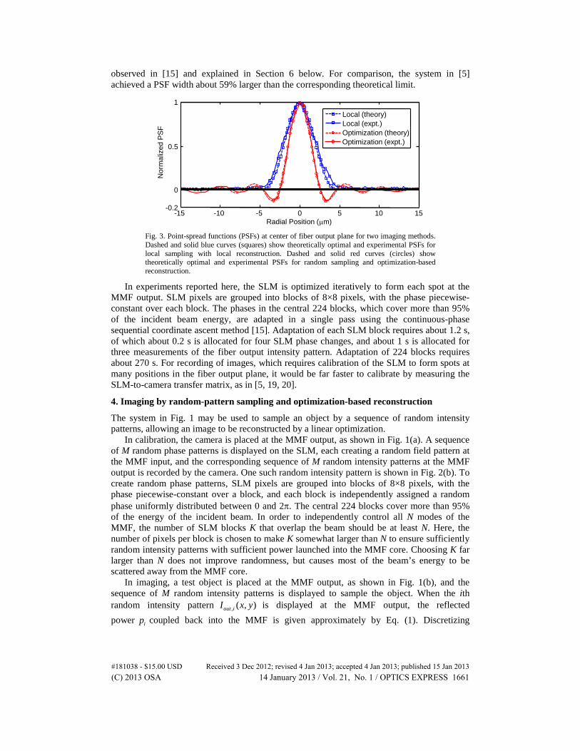
observed in [15] and explained in Section 6 below. For comparison, the system in [5] achieved a PSF width about 59% larger than the corresponding theoretical limit.

-15 -10 -5 0 5 10 15-0.2

0

0.5

Radial Position (µm)

Nor

mal

ized

PS

F

1

Optimization (theory)

Local (theory)

Optimization (expt.)

Local (expt.)

Fig. 3. Point-spread functions (PSFs) at center of fiber output plane for two imaging methods. Dashed and solid blue curves (squares) show theoretically optimal and experimental PSFs for local sampling with local reconstruction. Dashed and solid red curves (circles) show theoretically optimal and experimental PSFs for random sampling and optimization-based reconstruction.

In experiments reported here, the SLM is optimized iteratively to form each spot at the MMF output. SLM pixels are grouped into blocks of 8×8 pixels, with the phase piecewise-constant over each block. The phases in the central 224 blocks, which cover more than 95% of the incident beam energy, are adapted in a single pass using the continuous-phase sequential coordinate ascent method [15]. Adaptation of each SLM block requires about 1.2 s, of which about 0.2 s is allocated for four SLM phase changes, and about 1 s is allocated for three measurements of the fiber output intensity pattern. Adaptation of 224 blocks requires about 270 s. For recording of images, which requires calibration of the SLM to form spots at many positions in the fiber output plane, it would be far faster to calibrate by measuring the SLM-to-camera transfer matrix, as in [5, 19, 20].

4. Imaging by random-pattern sampling and optimization-based reconstruction

The system in Fig. 1 may be used to sample an object by a sequence of random intensity patterns, allowing an image to be reconstructed by a linear optimization.

In calibration, the camera is placed at the MMF output, as shown in Fig. 1(a). A sequence of M random phase patterns is displayed on the SLM, each creating a random field pattern at the MMF input, and the corresponding sequence of M random intensity patterns at the MMF output is recorded by the camera. One such random intensity pattern is shown in Fig. 2(b). To create random phase patterns, SLM pixels are grouped into blocks of 8×8 pixels, with the phase piecewise-constant over a block, and each block is independently assigned a random phase uniformly distributed between 0 and 2π. The central 224 blocks cover more than 95% of the energy of the incident beam. In order to independently control all N modes of the MMF, the number of SLM blocks K that overlap the beam should be at least N. Here, the number of pixels per block is chosen to make K somewhat larger than N to ensure sufficiently random intensity patterns with sufficient power launched into the MMF core. Choosing K far larger than N does not improve randomness, but causes most of the beam’s energy to be scattered away from the MMF core.

In imaging, a test object is placed at the MMF output, as shown in Fig. 1(b), and the sequence of M random intensity patterns is displayed to sample the object. When the ith random intensity pattern , ( , )out iI x y is displayed at the MMF output, the reflected power ip coupled back into the MMF is given approximately by Eq. (1). Discretizing


the ( , )x y plane at the MMF output into a grid of L pixels with spacing x y∆ = ∆ , with the kth pixel centered at ( , )k kx y , the integral in Eq. (1) can be approximated as a summation:

,1

( , ) ( , ) ,L

i out i k k obj k kk

p I x y R x yκ=

≈ ∑ (4)

where x yκ κ= ∆ ∆ is the normalized coupling coefficient. In order to reconstruct an image, we define p to be an 1M × vector whose ith entry

is ip and define I to be an M×L matrix whose ith row is , ( , )out i k kI x y . An image ( , )W x y in

discretized form ( , )k kW x y is represented as an 1L× vector w whose kth entry is ( ),k kW x y . The reconstructed image w is obtained by solving a linear optimization problem:

2

ˆ arg min ,= −w

w p Iw (5)

where2

denotes an l2-norm. Intuitively, w represents the object reflectivity pattern which, if

sampled by the intensity patterns I , would yield samples closest to the observed samples p. The solution to Eq. (5) is given by [24]:

1ˆ ,T−=w VD U p (6)

where superscript T denotes matrix transpose, and T=I UDV is the compact singular value decomposition of I . V is an L Q× matrix of the first Q right singular vectors of I and 1−D is a

Q Q× diagonal matrix of the reciprocals of the Q singular values of I . After w is computed

using Eq. (6), yielding a corresponding ˆ ( , )k kW x y , the reconstructed image is

1ˆ ˆ( , ) ( , ) ( , )

L

k k kkW x y W x y s x y

== ∑ , where ( , )ks x y is defined below Eq. (2). Unlike the object

reflectivity ( , )obj k kR x y , the reconstructed image ˆ ( , )k kW x y is not constrained to be

nonnegative everywhere, so any negative values in ˆ ( , )k kW x y are set to zero. The number of singular values Q corresponds to the number of resolvable image features,

as explained further in Section 5. As shown there, for a MMF supporting a large number of modes N, the number of resolvable features Q can be as high as 4N. Achieving this resolution obviously requires a number of random intensity patterns and a number of pixels at least that large, i.e., 4M N≥ and 4L N≥ .

The idealized PSF for random-pattern sampling with optimization-based reconstruction is discussed in Section 6. In a graded-index MMF, the PSF shape and width varies as a function of the pixel coordinate ( , )k kx y . It is narrowest at the center of the output plane where, in the limit of many modes N, it ideally approaches a diffraction-limited Airy disk:

10

2 (2 )(2 ) ,

2AJ rE r E

rη

ηη

= (7)

where 2 4 NA /η π λ= and 0E is a normalization constant. Like Eq. (3) the ideal PSF on Eq. (7) depends only on / NAλ and not on N. Its peak-to-zero width is 0.3 / NAλ , precisely half that of Eq. (3), while its HWHM is 0.18 / NAλ , about 0.69 times that of Eq. (3). The ideal PSF in Eq. (7) for our system is shown by the dashed red curve in Fig. 3, and has peak-to-zero width of 2.5 µm and HWHM of 1.4 µm. To estimate the PSF for our experimental system, we observe that if the object reflectivity ( , )obj k kR x y is set to unity for k l= and zero otherwise,


then p is the lth column of I , and the reconstructed image corresponds to the PSF for an object point at ( , )l lx y . This method has been used to compute the solid red curve in Fig. 3, which is in excellent agreement with the idealized PSF in Eq. (7). In estimating the PSF, 3000 random patterns have been used, and only the strongest 131 singular values have been used to minimize the effect of noise.

Figure 4 shows experimental images of chrome-on-glass objects from groups 6 and 7 of a USAF 1951 resolution target. Using random-pattern sampling and optimization-based reconstruction, all four objects are resolved, including bars with pitches of 9.8, 6.2 and 4.4 µm. This is to be expected, since all pitches exceed the experimental estimate of the PSF peak-to-zero width of 2.5 µm. By contrast, when using spot scanning and local reconstruction, the bars with 6.2-µm pitch are barely resolvable, while those with 4.4-µm pitch are not resolvable, consistent with the PSF peak-to-zero width of well over 5.0 µm. Each image in Fig. 4 represents an average of 15 preliminary images, each recorded using a different sequence of M = 200 random patterns, and has L = 75×75 = 5625 pixels. As explained in Section 5, in this fiber with N = 45 modes, up to 153 image features may be resolvable. In order to minimize noise, only the strongest 131 singular values are used in the images of Fig. 4.

-20 -10 0 10 20-20

-10

0

10

20

x (µm)

y ( µ

m)

-20 -10 0 10 20-20

-10

0

10

20

x (µm)

y ( µ

m)

-20 -10 0 10 20-20

-10

0

10

20

x (µm)

y ( µ

m)

-20 -10 0 10 20-20

-10

0

10

20

x (µm)

y ( µ

m)

(a) (b)

(c) (d)

Fig. 4. Images formed by random-pattern sampling and optimization-based reconstruction: (a) numeral 2, (b) bars of 9.8-µm pitch, (c) bars of 6.2-µm pitch, (d) bars of 4.4-µm pitch. Using the spot-scanning method with local reconstruction, (a) and (b) are easily resolved, (c) is barely resolved, while (d) is not resolved. Features are from groups 6 and 7 of 1951 USAF chrome-on-glass resolution target. Portions of other features can be seen in images (c) and (d). The white circle denotes the area in which spots and random patterns can be generated. A gamma adjustment of 1.5 is used in displaying the images.

Experiments reported here employ extensive averaging to minimize noise. In calibration, 20 camera frames are averaged for each random pattern, requiring 82 min for 3000 patterns. In imaging, 20 power meter readings are averaged for each random pattern, requiring 36 min for 3000 patterns. Reconstruction of a 75×75-pixel image (similar to the images in Fig. 4) requires 12 s. Redesign of the apparatus can significantly speed up calibration, imaging and reconstruction, while improving resolution, as described in Section 7.

5. Number of resolvable features

In this section, we explain how optimization-based reconstruction allows resolution of up to 4N image features, the factor of four becoming exact for large N. We show that at the output


of an N-mode fiber, an ensemble of electric field patterns has a dimensionality of at most N, whereas an ensemble of intensity patterns has a dimensionality up to 4N. Optimization-based reconstruction can exploit this full dimensionality of 4N, whether the intensity patterns are localized spots or random. By contrast, local reconstruction requires localized spot patterns, so it can only resolve N image features. The fourfold resolution enhancement corresponds to a twofold reduction in the width of the PSF at the center of the fiber output plane.

A graded-index MMF with finite core diameter d supports 2(1/ 8)N V= = 2(1/ 8)( NA / )dπ λ electric field modes per polarization for large V [25]. Here we consider

propagation of a finite but large number of modes N in a fiber having an infinite parabolic index profile. In polar coordinates ( , )r ϕ , the modes can be approximated well by Laguerre-Gaussian modes [25]. Without loss of generality we can consider the modes in the plane z = 0, allowing us to ignore z-dependent phase factors and write:

220

2

20 0 0

2 2( , ) ,r

w

ll illm

lm mc r rE r e L ew w w

ϕϕ−

= (8)

where ( )lmL ⋅ is the generalized Laguerre polynomial, 0 2 NAw dλ π= is the mode radius,

( )2 !/ !lmc m l mπ= + is a normalization constant and max0 2 2m l n N≤ + ≤ = .

Using an SLM, any linear combination of these modes can be generated at the fiber output, so the total output field distribution can be described by:

220

max max

2

20 00 2 0 2

2 2( , ) ( , ) ,r

w

l mil

out lm lm lmm l n m l n

r rE r a E r e a ew w

ϕϕ ϕ−

≤ + ≤ ≤ + ≤

= =

∑ ∑ (9)

where the lma can be obtained from the lma . Since 2max / 2N n= , the total number of “field

modes” N is proportional to the square of the upper limit of summation nmax. The output intensity distribution is the squared modulus of Eq. (9):

2220

max max

2

20 00 2 2 0 2 2

2 2( , ) ( ) ( , ) ,r

w

l mil il

out lm lm lm lmm l n m l n

r rI r e b e b e b E rw w

ϕ ϕϕ ϕ−

∗ −

≤ + ≤ ≤ + ≤

= + =

∑ ∑ (10)

where the lmb can be obtained from the lma and the lmb can be obtained from the lmb . The output intensity distribution in Eq. (10) is a linear combination of Laguerre-Gaussian modes with mode radius reduced to 0 / 2w . Since the upper limit of summation is 2nmax, the total number of “intensity modes” is 4N.

All 4N degrees of freedom can be exploited by the optimization-based reconstruction in Eq. (6). Using Eq. (4), neglecting noise, the vector of reflected powers can be written as

=p Ir , where r is an 1L× vector representing the object reflectivity values ( , )obj k kR x y in the L pixels. Then Eq. (6) takes the form:

1ˆ ,T−=w VD U Ir (11)

which simplifies to:

ˆ .T=w VV r (12)

Each of the Q rows of VT corresponds to an “intensity mode” of the fiber, recovered from the random intensity pattern matrix I . The object r is thus projected into the space spanned by


linear combinations of Q orthogonal “intensity modes” of the fiber. Neglecting noise, all components of the object corresponding to these Q “intensity modes” appear in the image w with unit gain, while other components are passed with zero gain and do not appear in the image.

Neglecting noise, based on Eq. (10), we expect the number of significant singular values of the matrix of field patterns to be approximately N, and the number of significant singular values Q of the matrix of intensity patterns to approach 4N, regardless of whether the patterns are random or represent localized spots. This is verified by Fig. 5, which presents simulations for the experimental apparatus of Fig. 1, which uses a graded-index MMF supporting N = 45 modes. The exact LP modes of the finite-core fiber are used, and an ensemble of 500 patterns is used in each matrix. Random or localized electric field patterns, shown in Fig. 5(a), have 45 significant singular values. The corresponding intensity patterns, shown in Fig. 5(b), have 153 significant singular values (153 is the precise number of “intensity modes” obtained by squaring linear combinations of 45 “field modes”). Figure 5(b) also shows singular values measured experimentally for an ensemble of 500 random intensity patterns. These do not exhibit a sharp drop at 153, presumably because of noise. In our experimental images shown in Fig. 4, we use only singular values that are at least 1% (−20 dB) with respect to the largest, resulting in 131 usable singular values.

0 50 100 150 200

-150

-100

-50

0

Singular Value Number0 50 100 150 200

-150

-100

-50

0

Singular Value Number

(a) Electric Field (b) Intensity

10 lo

g 10(

|SV|

) (dB

)

Random (simul.)Spot (simul.)Random (expt.)

Fig. 5. Singular values (SVs) for (a) electric field patterns and (b) intensity patterns at the output of a 45-mode graded-index MMF. Red circles and blue squares show SVs of random patterns and spots, respectively, simulated using the exact LP modes of finite-core MMF. Green diamonds denote SVs of random patterns measured experimentally. 500 patterns are used in each matrix.

A step-index MMF supports 2 2(1/ 4) (1/ 4)( NA / )N V dπ λ= = modes for large N, twice as many as a graded-index fiber having the same normalized frequency V [26]. Simulations of step-index fibers show results similar to Fig. 5, i.e., they confirm that the number of singular values of intensity patterns (and thus the number of resolvable image features) approaches 4N.

6. Point-spread function

In this section, we show analytically that in graded-index MMF, the idealized PSFs at the center of the output plane are given by Eq. (3) for local sampling and reconstruction and by Eq. (7) for optimization-based reconstruction. Using simulation, we compare the PSFs for optimization-based reconstruction in graded-index and step-index MMFs, showing how they vary with position in the fiber output plane.

We discuss optimization-based reconstruction first, deriving the idealized PSF in Eq. (7). By definition, the PSF is the reconstructed image obtained when the test object reflectivity

( , )objR x y is an ideal impulse ( , )x yδ and noise is negligible. Based on the optimization method in Eq. (5), this PSF should be an approximation of ( , ) ( ) /x y r rδ δ= using the set of 4N “intensity modes” appearing in Eq. (10) that minimizes the L2-norm of the approximation error. As shown in [15, Eq. (A4)], this approximation ( , )E rδ ϕ is a linear combination of the


“intensity modes” with coefficients equal to the complex-conjugated samples of the modes at the origin:

max0 2 2

( , ) (0,0) ( , ).lm lmm l n

E r E E rδ ϕ ϕ∗

≤ + ≤

= ∑ (13)

We would like to show that ( , )E rδ ϕ given by Eq. (13) approaches the Airy disk in Eq. (7) in the limit of a large number of “intensity modes”.

Using Eq. (8), (0,0)lmE∗ is nonzero only for 0l = and hence ( , )E rδ ϕ has no ϕ dependence

and can be written as:

22max max2

02

00 0 2 2

0 00 0

2 4( ) (0,0) ( , ) .r

wn n

m m mm m

rE r E E r e Lw wδ ϕ

π

−

∗

= =

= =

∑ ∑ (14)

According to the Heine-Mehler theorem, for any large n we have [27]:

( )/2 /2/2

( )2 .rnL r

e r J nrn

αα

αα−= (15)

Letting 1α = , replacing r by 2 2 /r nη and rearranging, we get:

2 2 /2 2 2

112 (2 ).

2

r n

nJ r e rL

r n n

ηη ηη

− =

(16)

Using properties of Laguerre polynomials we have 1 0

0( ) ( )

n

n mmL r L r

== ∑ so that:

2 2 /2 2 2

01

0

2 (2 ).

2

nr n

mm

J r e rLr n n

ηη ηη

−

=

=

∑ (17)

Setting 2 20 / 4n wη= and 2

0 / 2E η π= we get:

22 max2

02

0 102 2

0 00

2 (2 )2 4( ) (2 ).2

rw

n

m Am

J rrE r e L E E rrw wδη

ηηπ

−

=

= = =

∑ (18)

Hence, in the limit of a large number of “intensity modes”, the optimization-based PSF at the center of the fiber output plane converges to the Airy disk in Eq. (7), whose width depends only on 2 4 NA /η π λ= . Although Eq. (7) represents an incoherent PSF, its functional form is suggestive of the coherent PSF of a conventional imaging system having an NA twice that of the fiber [28]. Since Eq. (7) arises from a computational reconstruction process, it is not constrained to be nonnegative everywhere in the fiber output plane, unlike a PSF arising from conventional physical incoherent imaging.

In a system using local sampling and reconstruction, the idealized PSF at the center of the fiber output plane is the narrowest intensity pattern , ( , )out iI x y that can be formed there. As shown in [15], the corresponding field pattern is the approximation of ( , ) ( ) /x y r rδ δ= using the set of N “field modes” that minimizes the L2-norm of the approximation error. Following the arguments given above, replacing η by / 2η , maxn by max / 2n , and 0w by 02w , this field

pattern is 0 1( / 4)2 ( ) /E J r rη η and its square is the PSF ( )20 1( ) 2 ( ) /AI r I J r rη η η= given in Eq.

(3).


Through simulation, we have studied the PSFs in fibers with different index profiles and at different positions in the fiber output plane. We modeled the exact LP modes in fibers having NA = 0.19 and core diameter d = 50 µm, like the experimental system in Fig. 1. Graded-index and step-index fibers support N = 45 and 94 modes, respectively. Using random-pattern sampling with optimization-based reconstruction, at the center of the fiber output plane, the shape and width of PSFs for graded-index or step-index fibers are both very similar to the idealized PSF in Eq. (7), shown in Fig. 3 by the dashed red line, despite the roughly twofold disparity in number of propagating modes. Figure 6 presents PSF widths for centroid positions displaced from the center of the output plane for the two fiber types. The transverse and longitudinal directions are parallel and perpendicular to the direction of displacement, respectively. In graded-index fibers the PSF widths (blue lines) increase from the ideal limit at points away from the center of the output plane, whereas in step-index fibers the PSF widths (red lines) are close to the ideal limit over the entire range. This observed difference is consistent with the roughly twofold disparity in the number of modes and the corresponding number of observable features.

0 10 200

2.5

5.0

7.5

PSF Centroid Position (µm)

PS

FP

eak-

to-Z

ero

Wid

th (µ

m)

SI (longitudinal)SI (transverse)GI (longitudinal)GI (transverse)

Idealized PSF

Fig. 6. Peak-to-zero widths of PSFs for optimization-based reconstruction at different radial positions in the fiber output plane. Dashed and solid blue lines (squares) show transverse and longitudinal widths for the graded-index fiber. Dashed and solid red lines (circles) show transverse and longitudinal widths for the step-index fiber. PSFs were obtained from simulation of a noiseless random-pattern imaging system with optimization-based reconstruction using exact LP modes of fibers having NA = 0.19 and core diameter d = 50 µm. The dashed black line corresponds to idealized PSF given by Eq. (7).

Analogous results are observed for local sampling and reconstruction. At the center of the fiber output plane, the PSFs for graded-index and step-index fibers are both very similar to the idealized PSF in Eq. (3), shown by the dashed blue line in Fig. 3. In graded-index fibers, the PSF widths increase at points away from the center of the output plane, but in step-index fibers, the PSF widths remain nearly constant for displacements beyond 20 µm.

For either imaging method, the relationship between the PSF and the number of resolvable features can be understood intuitively in step-index fibers, where the PSF shape and width are nearly invariant over the fiber output plane. Under the Rayleigh criterion [29], two object points are resolvable if their spacing is at least equal to the peak-to-zero width of the appropriate PSF (given by Eq. (7) or Eq. (3) for optimization-based or local reconstruction, respectively). Arraying a hexagonal lattice of points with such spacing, one finds that the fiber core encloses 1.02N or 4.07N lattice points for optimization-based or local reconstruction, respectively. These are very close to the N or 4N resolvable features found by the rigorous analysis in Section 5.

7. Discussion

Random-pattern sampling with optimization-based reconstruction may be considered somewhat analogous to local sampling and reconstruction with deconvolution. In the latter method, after local reconstruction, deconvolution involves multiplying the reconstructed


image spatial frequency spectrum by the inverse transfer function of the imaging system, assuming the PSF is approximately spatially invariant [30], as in step-index fiber. If the PSF is spatially variant, as in graded-index fiber, deconvolution is possible, but becomes much more complicated [31]. In either case, deconvolution sharpens the image by enhancing spatial frequencies approaching the incoherent cutoff, but leads to noise enhancement. Similarly, in the former method, optimization-based reconstruction in Eq. (6) includes multiplication by the matrix D−1, which compensates for the diminishing singular values of the intensity pattern matrix I approaching the incoherent cutoff, but leads to noise enhancement. We have not yet fully compared the two methods in terms of the tradeoff between resolution and noise enhancement. In the former method, this tradeoff may perhaps be optimized by designing a set of intensity patterns having minimal variation among the singular values.

The experimental apparatus in Fig. 1, designed originally for data transmission at 1550 nm [32] and retrofitted at minimal cost for imaging experiments [15], has several limitations that significantly compromise image resolution and noise levels and slow down calibration and image acquisition. These include the long wavelength, graded-index fiber, SLM (slow interface and switching speed), phosphor-coated CCD camera (low frame rate, poor sensitivity, high noise level, slow interface), power meter (slow interface) and PC. If the system were redesigned to use a 532-nm wavelength and 50-µm, NA = 0.19, step-index fiber supporting N = 787 modes, it would achieve a resolution of 0.3λ/NA ≈ 0.84 µm over most of the fiber output plane, corresponding to 4N = 3148 resolvable features. Using a high-speed SLM, high-frame-rate CCD camera and high-performance PC, estimated times for calibration, image recording and reconstruction are 11.5 min, 17 s and 10 s.

8. Conclusion

We have demonstrated a method for imaging through an N-mode fiber that can resolve up to 4N image features. An SLM forms a sequence of at least 4N random input field patterns, which create a sequence of random intensity patterns for sampling an object placed at the fiber output. Reflected power values are returned through the fiber and an image is reconstructed by linear optimization. Although the 4N field patterns span the set of N “field modes”, the squaring inherent in field-to-intensity conversion mixes the modes, so the intensity patterns span a set of 4N “intensity modes”. Most previous fiber imaging methods use localized intensity patterns for sampling and use local reconstruction, and all of them can only resolve N image features. The number of modes N, and thus the number of image features resolvable by these methods (4N or N) depend on the square of the normalized frequency NA /V dπ λ= and on the fiber refractive index profile. Nevertheless, the shape and width of the PSF at the center of the fiber output plane appear to depend only on / NAλ . Experiments described here used graded-index fibers with d = 50 mm and NA = 0.19 supporting N = 45 modes at λ = 1550 nm. Resolution may be enhanced in future experiments using larger-diameter, higher-NA step-index fibers and shorter optical wavelengths.

Acknowledgments

The authors are grateful for discussions with B. Babadi, E. Candes, J. W. Goodman, D. A. B. Miller and J. P. Wilde. This research was supported by a Stanford Graduate Fellowship and Corning, Inc.


Documents

Res.limits.fiber.imaging.opex.1 13