Full Terms & Conditions of access and use can be found athttp://www.tandfonline.com/action/journalInformation?journalCode=tgei20

Download by: [199.133.74.86] Date: 25 September 2015, At: 10:34

Geocarto International

ISSN: 1010-6049 (Print) 1752-0762 (Online) Journal homepage: http://www.tandfonline.com/loi/tgei20

Use of Kendall's coefficient of concordance toassess agreement among observers of very highresolution imagery

Amanda Gearhart , D. Terrance Booth , Kevin Sedivec & Christopher Schauer

To cite this article: Amanda Gearhart , D. Terrance Booth , Kevin Sedivec & ChristopherSchauer (2013) Use of Kendall's coefficient of concordance to assess agreement amongobservers of very high resolution imagery, Geocarto International, 28:6, 517-526, DOI:10.1080/10106049.2012.725775

To link to this article: http://dx.doi.org/10.1080/10106049.2012.725775

Accepted online: 20 Sep 2012.Publishedonline: 22 Jan 2013.

Submit your article to this journal

Article views: 149

View related articles

Citing articles: 2 View citing articles

Use of Kendall’s coefficient of concordance to assess agreement among

observers of very high resolution imagery

Amanda Gearharta*, D. Terrance Boothb, Kevin Sedivecc and Christopher Schauerd

aEastern Oregon Agricultural Research Center, USDA-ARS, 67826-A Hwy 205, Burns 97720,USA; bHigh Plains Grasslands Research Station, USDA-ARS, 8408 Hildreth Road, Cheyenne82009, USA; cSchool of Natural Resource Sciences, North Dakota State University, P.O. Box6050, Fargo 58108-6050, USA; dHettinger Research Extension Center, North Dakota State

University, P.O. Box 1377, Hettinger 58639-1377, USA

(Received 3 May 2012; final version received 28 August 2012)

Ground-based vegetation monitoring methods are expensive, time-consumingand limited in sample size. Aerial imagery is appealing to managers because of thereduced time and expense and the increase in sample size. One challenge of aerialimagery is detecting differences among observers of the same imagery. Sixobservers analysed a set of 1-mm ground sample distance aerial imagery forgraminoid species composition and important ground-cover characteristics.Kendall’s coefficient of concordance (W) was used to measure agreement amongobservers. The group of six observers was concordant when assessed as a group.When each of the observers was assessed independently against the other five,lack of agreement was found for those graminoid species that were difficult toidentify in the aerial images.

Keywords: 1-mm GSD imagery; grassland monitoring; rangeland monitoring;SamplePoint; very large scale aerial imagery

1. Introduction

Monitoring natural ecosystems has been the subject of a plethora of books, manualsand articles for many decades (e.g. Clements 1928, Levy and Madden 1933, Canfield1941, ‘t Mannetje and Haydock 1963, Senay and Elliot 2000, Wang et al. 2004,Toevs et al. 2011). This is particularly true of public rangelands due to their vast areaand federal mandates requiring vegetative monitoring. On-the-ground monitoringrequiring the physical presence of professionals in the field is considered the standardfor monitoring rangelands; however, the type of terrain, geographical area to becovered, number of professionals available, methods used and funding all limit thenumber of plots that can feasibly be monitored in one growing season by traditionalmethods (Owens et al. 1985, Pellant et al. 1999, West 1999, Booth and Tueller 2003,Forbis et al. 2007).

Aerial imagery is appealing to managers for a number of reasons. Firstly, thesample size (i.e. the number of plots) can be increased dramatically without incurringsubstantial additional expense. Secondly, images are a record of resource conditions

*Corresponding author. Email: amandag@uidaho.edu

http://dx.doi.org/10.1080/10106049.2012.725775

� 2013 Taylor & Francis

Geocarto International 2013Vol. 28, No. 6, 517–526,

,

Dow

nloa

ded

by [

] at

10:

34 2

5 Se

ptem

ber

2015

that can be re-examined, whereas traditional non-imaging methods record fieldobservations without a practical means of verification and exclude the possibility ofre-sampling present conditions at a future date. However, the use of imaging methodsto provide a means for data verification depends on the ability of observers to inter-pret images of resource conditions in the same way – that is, to have concordance.

Any type of monitoring, whether ground- or imagery-based, is not withoutdisadvantages. There are many types of errors associated with monitoring (e.g.between years [Kennedy and Addison 1987], methods [Whitman and Siggiersson1954, Kercher et al. 2003] and plot sizes [Klimes 2003, Heywood and DeBacker2007]). Our research focused on detecting differences among observers (Smith 1944,Brakenhielm and Qinghong 1995, Booth et al. 2005, Vittoz and Guisan 2007).

Brakenhielm and Qinghong (1995) and Vittoz and Guisan (2007) utilized pairedt-tests to detect differences between observers, while Smith (1944) combined allobservers and used an analysis of variance (ANOVA) to determine differencesbetween the group of observers on different days. Booth et al. (2005) utilized anANOVA with mean separation test to detect differences among observers. A meanseparation test and Kappa statistic (a statistical measure of inter-rater agreement)can be appropriate analyses when n is small, but become cumbersome when n islarge. Additionally, w2 tests have a low Type I error and are overly conservative whenthe number of observers is less than 20 (Legendre 2004, 2005).

Kendall’s coefficient of concordance (W) is a measure that uses ranks to assessagreement between observers (Kendall and Babington Smith 1939) similar toSpearman’s rank correlation coefficient1 (1904). Our objective was to test the utilityof Kendall’s W for determining the level of agreement among six observers.

2. Methods

2.1. Study area

The imagery used in this study was collected in the Grand River National Grasslands(GRNG; lat. 458550 long. 1028320) near Hettinger, ND. The study area is a typicalmixed-grass prairie of the northern Great Plains of the central USA, characterized bywestern wheatgrass (Pascopyrum smithii [Rydb.] A. Love), blue grama (Boutelouagracilis [Willd. ex Kunth] Lag. ex Griffiths), needle and thread (Hesperostipa comata[Trin. &Rupr.] Barkworth), prairie junegrass (Koeleria macrantha [Ledeb.] Schult.) andthreadleaf sedge (Carex filifolia Nutt., Kuchler 1964, Hansen 2008, USDA NRCS2012). This area was heavily farmed during the first half of the twentieth century(Hansen 2008). Several non-native grasses are of concern in this area, including smoothbrome (Bromus inermis Leyss.), Kentucky bluegrass (Poa pratensis L.) and crestedwheatgrass (Agropyron cristatum [L.] Gaertn.), which was generally selected forreseeding efforts and has populated abandoned fields (USDA NRCS 2012).

2.2. Imagery

True colour, digital, very large scale aerial (VLSA) images were collected between 15July and 1 August 2007. These dates were selected to maximize the likelihood thatthe cool season graminoids would have inflorescence and warm season graminoidshave sufficient growth to be identifiable in the imagery. Images were acquired by asport aircraft (225 kg empty weight) at approximately 100 m above ground level and23.5 m s71 average ground speed (FAA 2004). A 16.7-megapixel Canon EOS 1DS

2 A. Gearhart et al.518

Dow

nloa

ded

by [

] at

10:

34 2

5 Se

ptem

ber

2015

Mark II (Canon USA, Lake Success, NY, 4992 6 3328 pixels) configured with an840-mm focal-length lens captured images with an average ground sample distance(GSD; a measure of digital image resolution) of approximately 1 mm and 3 6 4 mfield of view. Booth and Cox (2008) and Moffet (2009) described the equipment andsampling methods.

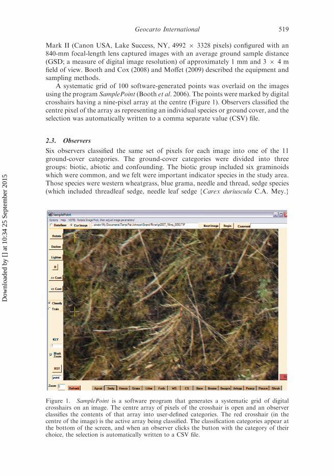
A systematic grid of 100 software-generated points was overlaid on the imagesusing the program SamplePoint (Booth et al. 2006). The points were marked by digitalcrosshairs having a nine-pixel array at the centre (Figure 1). Observers classified thecentre pixel of the array as representing an individual species or ground cover, and theselection was automatically written to a comma separate value (CSV) file.

2.3. Observers

Six observers classified the same set of pixels for each image into one of the 11ground-cover categories. The ground-cover categories were divided into threegroups: biotic, abiotic and confounding. The biotic group included six graminoidswhich were common, and we felt were important indicator species in the study area.Those species were western wheatgrass, blue grama, needle and thread, sedge species(which included threadleaf sedge, needle leaf sedge {Carex duriuscula C.A. Mey.}

Figure 1. SamplePoint is a software program that generates a systematic grid of digitalcrosshairs on an image. The centre array of pixels of the crosshair is open and an observerclassifies the contents of that array into user-defined categories. The red crosshair (in thecentre of the image) is the active array being classified. The classification categories appear atthe bottom of the screen, and when an observer clicks the button with the category of theirchoice, the selection is automatically written to a CSV file.

Geocarto International 3519

Dow

nloa

ded

by [

] at

10:

34 2

5 Se

ptem

ber

2015

and sun sedge {Carex inops L.H. Bailey ssp. heliophila [Mack.] Crins}), bluegrassspecies (which included Kentucky bluegrass, Sandberg’s bluegrass {Poa secunda J.Presl} and Canada bluegrass {Poa compressa L.}) and crested wheatgrass. Theabiotic group included three ground-cover categories generally considered importantindicators of ecological change (Booth and Cox 2008): bare ground (bare mineralsoil), litter (which included senesced plant material, duff and dung) and rock. Theconfounding group included two variables which were confusing to observers: grass(in which a specific graminoids species could not be determined) and shadow.

The observers were all females of various ages that had a range of on-the-groundfield experience in the study area (Table 1). We deliberately chose observers who hada range of experiences working with imagery, general field experience and study area-specific experience. All observers had at least 3 years of plant identificationexperience. Observers A, B and C were under 30 years of age and had at least 2 yearsof experience in the study area. Observers D, E and F were over 30 years of age andhad 5 days or less experience in the study area.

2.4. Statistical analysis

Kendall’s coefficient of concordance (W) was applied to observations from allobservers for each ground-cover category independently. Kendall’s W is calculatedby Equation (1):

W ¼ 12S

p2ðn3 � nÞ � pTð1Þ

where S is the sum-of-squares from row sums of ranks Ri (Equation (2)), n is thenumber of objects, p is the number of judges and T is a correction factor for tiedranks (Equation (3); Siegel 1956, p. 234).

S0 ¼Xn

i¼1R2

i ¼ SSR ð2Þ

T ¼Xm

k¼1ðt3k � tkÞ ð3Þ

where S is the sum-of-squares from row sums of ranks Ri, m is the number of groupsand tk is the number of tied ranks in each (k) of m groups (Siegel 1956, p. 234).

Table 1. Six observers classified a set of 146 one-millimetre GSD digital aerial images into 11ground-cover categories. The observers were all female, ranged in age from 18 to 55 years ofage and had various imagery, general field and study area-specific experience levels.

Characteristics and experiences

Observer

A B C D E F

Gender F F F F F FAge (years) 28 18 22 40 55 49SamplePoint/VLSA imagery

experience2 years 7 days 7 days 3 years 7 days 8 years

General field experience (years) 8 3 4 20 20 30Study area-specific experience 5 years 3 years 2 years 5 days 0 days 0 days

4 A. Gearhart et al.520

Dow

nloa

ded

by [

] at

10:

34 2

5 Se

ptem

ber

2015

This calculation was completed using the software program Kendall W which automa-tically transforms ordinal scores from each observer into cardinal ranks (Legendre2004, 2005). The overall null hypothesis of global concordance tested was that the sixobservers produced independent rankings for each ground-cover characteristic for allimages (i.e. the six observers were not concordant with one another). When thisglobal concordance hypothesis was rejected, we tested the a posteriori hypothesis ofindependent concordance that a specific observer produced a ground-cover character-istic ranking that was independent of the other five. The independent a posterioriconcordance tests were run with n ¼ 146 (number of images) and p ¼ 6 (number ofobservers). Concordance analyses were run independently for each of the 11 ground-cover categories with 9999 permutations to test the contribution of individual observersto the global concordance (W). Permutation testing is a more robust test than the w2 testand results in more accurate Type I error (Legendre 2005). Perfect agreement isindicated by values of 1, while no agreement is indicated by values of 0.

3. Results

3.1. Global concordance (W)

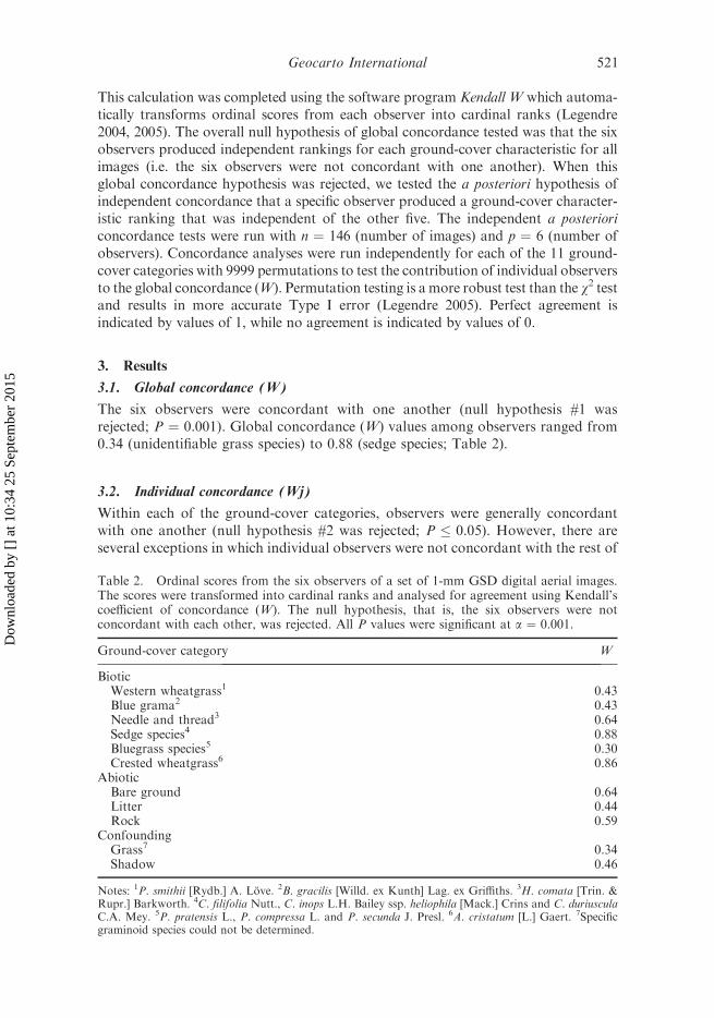
The six observers were concordant with one another (null hypothesis #1 wasrejected; P ¼ 0.001). Global concordance (W) values among observers ranged from0.34 (unidentifiable grass species) to 0.88 (sedge species; Table 2).

3.2. Individual concordance (Wj)

Within each of the ground-cover categories, observers were generally concordantwith one another (null hypothesis #2 was rejected; P � 0.05). However, there areseveral exceptions in which individual observers were not concordant with the rest of

Table 2. Ordinal scores from the six observers of a set of 1-mm GSD digital aerial images.The scores were transformed into cardinal ranks and analysed for agreement using Kendall’scoefficient of concordance (W). The null hypothesis, that is, the six observers were notconcordant with each other, was rejected. All P values were significant at a ¼ 0.001.

Ground-cover category W

BioticWestern wheatgrass1 0.43Blue grama2 0.43Needle and thread3 0.64Sedge species4 0.88Bluegrass species5 0.30Crested wheatgrass6 0.86

AbioticBare ground 0.64Litter 0.44Rock 0.59

ConfoundingGrass7 0.34Shadow 0.46

Notes: 1P. smithii [Rydb.] A. Love. 2B. gracilis [Willd. ex Kunth] Lag. ex Griffiths. 3H. comata [Trin. &Rupr.] Barkworth. 4C. filifolia Nutt., C. inops L.H. Bailey ssp. heliophila [Mack.] Crins and C. duriusculaC.A. Mey. 5P. pratensis L., P. compressa L. and P. secunda J. Presl. 6A. cristatum [L.] Gaert. 7Specificgraminoid species could not be determined.

Geocarto International 5521

Dow

nloa

ded

by [

] at

10:

34 2

5 Se

ptem

ber

2015

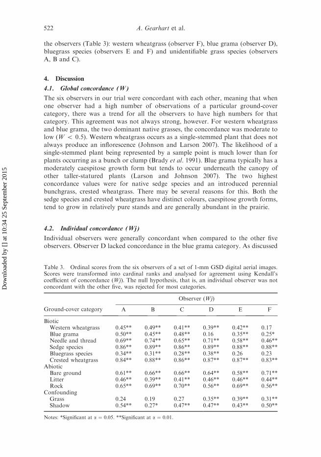
the observers (Table 3): western wheatgrass (observer F), blue grama (observer D),bluegrass species (observers E and F) and unidentifiable grass species (observersA, B and C).

4. Discussion

4.1. Global concordance (W)

The six observers in our trial were concordant with each other, meaning that whenone observer had a high number of observations of a particular ground-covercategory, there was a trend for all the observers to have high numbers for thatcategory. This agreement was not always strong, however. For western wheatgrassand blue grama, the two dominant native grasses, the concordance was moderate tolow (W 5 0.5). Western wheatgrass occurs as a single-stemmed plant that does notalways produce an inflorescence (Johnson and Larson 2007). The likelihood of asingle-stemmed plant being represented by a sample point is much lower than forplants occurring as a bunch or clump (Brady et al. 1991). Blue grama typically has amoderately caespitose growth form but tends to occur underneath the canopy ofother taller-statured plants (Larson and Johnson 2007). The two highestconcordance values were for native sedge species and an introduced perennialbunchgrass, crested wheatgrass. There may be several reasons for this. Both thesedge species and crested wheatgrass have distinct colours, caespitose growth forms,tend to grow in relatively pure stands and are generally abundant in the prairie.

4.2. Individual concordance (Wj)

Individual observers were generally concordant when compared to the other fiveobservers. Observer D lacked concordance in the blue grama category. As discussed

Table 3. Ordinal scores from the six observers of a set of 1-mm GSD digital aerial images.Scores were transformed into cardinal ranks and analysed for agreement using Kendall’scoefficient of concordance (Wj). The null hypothesis, that is, an individual observer was notconcordant with the other five, was rejected for most categories.

Ground-cover category

Observer (Wj)

A B C D E F

BioticWestern wheatgrass 0.45** 0.49** 0.41** 0.39** 0.42** 0.17Blue grama 0.50** 0.45** 0.48** 0.16 0.35** 0.25*Needle and thread 0.69** 0.74** 0.65** 0.71** 0.58** 0.46**Sedge species 0.86** 0.89** 0.86** 0.89** 0.88** 0.88**Bluegrass species 0.34** 0.31** 0.28** 0.38** 0.26 0.23Crested wheatgrass 0.84** 0.88** 0.86** 0.87** 0.87** 0.83**

AbioticBare ground 0.61** 0.66** 0.66** 0.64** 0.58** 0.71**Litter 0.46** 0.39** 0.41** 0.46** 0.46** 0.44**Rock 0.65** 0.69** 0.70** 0.56** 0.69** 0.56**

ConfoundingGrass 0.24 0.19 0.27 0.35** 0.39** 0.31**Shadow 0.54** 0.27* 0.47** 0.47** 0.43** 0.50**

Notes: *Significant at a ¼ 0.05. **Significant at a ¼ 0.01.

6 A. Gearhart et al.522

Dow

nloa

ded

by [

] at

10:

34 2

5 Se

ptem

ber

2015

in the previous section, blue grama may be difficult to correctly identify because itoccurs under the canopy of taller-statured plants. Observer F lacked concordance inthe western wheatgrass category. Western wheatgrass does not always produce aninflorescence and may be difficult to identify in imagery. Observers E and F bothlacked concordance for bluegrass species. The most common bluegrass that occurs inGRNG is Kentucky bluegrass (P. pratensis L.). Kentucky bluegrass can be difficultto identify, even on the ground. This introduced grass is strongly rhizomatous, doesnot always produce inflorescence and has narrow leaves (3.2–6.4 mm) that tend tofold or curl (Johnson and Larson 2007, USDA NRCS 2012).

Observers A, B and C lacked concordance in the unidentifiable grass category. Itmay be that Observers A, B and C were simply able to identify more grasses. It couldalso be that Observers D, E and F, who lacked concordance in individual speciescategories, placed those points into the unidentifiable grass category.

4.3. Environment

The northern mixed-grass prairie has a relatively continuous cover of grass that haschallenged individual species identification by remote sensing technologies for manyyears. This area is populated by both warm and cool season species which presentphenological challenges for point-in-time monitoring (e.g. the way this imagery wasused in this study). One of the advantages of aerial imagery is that additionalsampling periods could be added throughout the growing season to address thephenological changes occurring on the landscape.

The prairie canopy is heterogeneous and complex, containing a mix of tall-, mid-and short-statured species. This complexity may add to the difficulty of identifyingindividual species by canopy point sampling. Additionally, the local environmentalconditions of the GRNG made it difficult to get a quality set of imagery with theequipment used. Although wind speeds average 18 km h71 (UNL 2011), summer

Figure 2. Imagery collected on the GRNG during the summer of 2007 was subject toconsiderable motion blur due to wind gusts up to 30 km h71 that forced the sport aircraft totravel at higher speeds than preferable.

Geocarto International 7523

Dow

nloa

ded

by [

] at

10:

34 2

5 Se

ptem

ber

2015

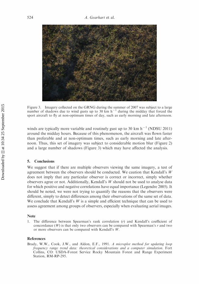
winds are typically more variable and routinely gust up to 30 km h71 (NDSU 2011)around the midday hours. Because of this phenomenon, the aircraft was flown fasterthan preferable and at non-optimum times, such as early morning and late after-noon. Thus, this set of imagery was subject to considerable motion blur (Figure 2)and a large number of shadows (Figure 3) which may have affected the analysis.

5. Conclusions

We suggest that if there are multiple observers viewing the same imagery, a test ofagreement between the observers should be conducted. We caution that Kendall’s Wdoes not imply that any particular observer is correct or incorrect, simply whetherobservers agree or not. Additionally, Kendall’s W should not be used to analyse datafor which positive and negative correlations have equal importance (Legendre 2005). Itshould be noted, we were not trying to quantify the reasons that the observers weredifferent, simply to detect differences among their observations of the same set of data.We conclude that Kendall’s W is a simple and efficient technique that can be used toassess agreement among groups of observers, especially when evaluating aerial images.

Note

1. The difference between Spearman’s rank correlation (r) and Kendall’s coefficient ofconcordance (W) is that only two observers can be compared with Spearman’s r and twoor more observers can be compared with Kendall’s W.

References

Brady, W.W., Cook, J.W., and Aldon, E.F., 1991. A microplot method for updating loopfrequency range trend data: theoretical considerations and a computer simulation. FortCollins, CO: USDA-Forest Service Rocky Mountain Forest and Range ExperimentStation, RM-RP-295.

Figure 3. Imagery collected on the GRNG during the summer of 2007 was subject to a largenumber of shadows due to wind gusts up to 30 km h71 during the midday that forced thesport aircraft to fly at non-optimum times of day, such as early morning and late afternoon.

8 A. Gearhart et al.524

Dow

nloa

ded

by [

] at

10:

34 2

5 Se

ptem

ber

2015

Brakenhielm, S. and Qinghong, L., 1995. Comparison of field methods in vegetationmonitoring. Water, Air and Soil Pollution, 79, 75–87.

Booth, D.T. and Cox, S.E., 2008. Image-based monitoring software to measure ecologicalchange in rangelands. Frontiers in Ecology and the Environment, 6, 185–190.

Booth, D.T. and Tueller, P.T., 2003. Rangeland monitoring using remote sensing. Arid LandResearch and Management, 17, 455–467.

Booth, D.T., Cox, S.E., and Johnson, D.E., 2005. Detection calibration and other factorsinfluencing digital measurements of ground cover. Rangeland Ecology and Management,58, 598–604.

Booth, D.T., Cox, S.E., and Berryman, R.D., 2006. Point sampling digital imagery with‘SamplePoint’. Environmental Monitoring and Assessment, 123, 97–108.

Canfield, R.H., 1941. Application of line interception method in sampling range vegetation.Journal of Forestry, 39, 388–394.

Clements, F.E., 1928. Plant succession and indicators: a definitive edition of plant succession andplant indicators. New York, NY: H.W. Wilson.

Federal Aviation Administration (FAA), 2004. Airworthiness certification of aircraft andrelated products. Order 8130.2F.

Forbis, T.A., et al., 2007. A method for landscape-scale assessment: application to Great Basinrangeland ecosystems. Rangeland Ecology and Management, 60, 209–217.

Hansen, K., 2008. Plants of the Grand River National Grasslands: 2008. USDA-Forest Service,Dakota Prairie Grasslands, internal report, 56 pp.

Heywood, J.S. and DeBacker, M.D., 2007. Optimal sampling designs for monitoring plantfrequency. Rangeland Ecology and Management, 60, 426–434.

Kendall, M.G. and Babington Smith, B., 1939. The problem of m rankings. The Annals ofMathematical Statistics, 10, 275–287.

Kennedy, K.A. and Addison, P.A., 1987. Some considerations for the use of visual estimatesof plant cover in biomonitoring. Journal of Ecology, 75, 151–157.

Kercher, S.M., Frieswyk, C.B., and Zedler, J.B., 2003. Estimates of sampling teams andestimation methods on the assessment of plant cover. Journal of Vegetation Science, 14,899–906.

Klimes, L., 2003. Scale-dependent variation in visual estimates of grassland plant cover.Journal of Vegetation Science, 14, 815–821.

Kuchler, A.W., 1964. Potential natural vegetation of the coterminous United States. New York,NY: American Geographical Company.

Johnson, J.R. and Larson, G.E., 2007. Grassland plants of South Dakota and the NorthernGreat Plains. Revised ed. Brookings, SD: South Dakota State University, College ofAgriculture and Biological Sciences, South Dakota Agricultural Experiment Station B566.

Larson, G.E. and Johnson, J.R., 2007. Plants of the Black Hills and Bear Lodge Mountains.2nd ed. Brookings, SD: South Dakota State University, College of Agriculture andBiological Sciences, South Dakota Agricultural Experiment Station B732.

Legendre, P., 2004. Kendall coefficient of concordance: global test and a posteriori tests ofindividual judges 7 program Kendall_W user’s guide. Departement de sciences biologiques,Universite de Montreal, 8 pp.

Legendre, P., 2005. Species associations: the Kendall coefficient of concordance revisited.Journal of Agricultural, Biological and Environmental Statistics, 10, 226–245.

Levy, E.B. and Madden, E.A., 1933. The point method of pasture analysis. New ZealandJournal of Agriculture, 46, 267–279.

Moffet, C.A., 2009. Agreement between measurements of shrub cover using ground-basedmethodsandvery large scale aerial imagery.RangelandEcologyandManagement, 62,268–277.

North Dakota State University (NDSU), 2011. North Dakota agricultural weather network.Available from: http://ndawn.ndsu.nodak.edu/ [Accessed 2 May 2011].

Owens, M.K, Gardiner, H.G. and Norton, B.E., 1985. A photographic technique for repeatedmapping of rangeland plant populations in permanent plots. Journal of Range Manage-ment, 38, 231–232.

Pellant, M., Shaver, P., and Spaeth, K. 1999. Field test of a prototype rangeland inventoryprocedure in the western USA. In: D. Eldridge and D. Freudenberger, eds. People andrangelands: building the future. Proceedings of the VI International Rangeland Congress, 19–23July1999.Townsville,Queensland,Australia:VI InternationalRangelandCongress, 766–767.

Geocarto International 9525

Dow

nloa

ded

by [

] at

10:

34 2

5 Se

ptem

ber

2015

Senay, G.B. and Elliot, R.L., 2000. Combining AVHRR NDVI and landuse data to describetemporal and spatial dynamics of vegetation. Forest Ecology and Management, 28, 83–91.

Siegel, S., 1956. Nonparametric statistics for the behavioral sciences. New York, NY: McGrawHill.

Smith, A.D., 1944. A study of the reliability of range vegetation estimates. Ecology, 25, 441–448.

Spearman, C., 1904. The proof and measurement of association between two things. TheAmerican Journal of Psychology, 15, 72–101.

’t Mannetje, L. and Haydock, K.P., 1963. The dry-weight-rank method for botanical analysisof pasture. Journal of the British Grassland Society, 18, 268–275.

Toevs, G.R., et al., 2011. Bureau of land management assessment, inventory, and monitoringstrategy: for integrated renewable resources management. Denver, CO: Bureau of LandManagement, National Operations Center, BLM/WO/GI-11/014þ1735.

United States Department of Agriculture Natural Resources Conservation Service (USDANRCS), 2012. The PLANTS database. Available from: http://plants.usda.gov [Accessed20 March 2012].

University of Nebraska Lincoln (UNL), 2011. High Plains Regional Climate Center. Availablefrom: http://www.hprcc.unl.edu/index.php [Accessed 14 January 2011].

Vittoz, P. and Guisan, A., 2007. How reliable is the monitoring of permanent vegetation plots?A test with multiple observers. Journal of Vegetation Science, 18, 413–422.

Wang, C., et al., 2004. Soil moisture estimation in a semiarid rangeland using ERS-2 and TMimagery. Remote Sensing of Environment, 90, 178–189.

West, N.E., 1999. Accounting for rangeland resources over entire landscapes. In: D. Eldridgeand D. Freudenberger, eds. People and rangelands: building the future. Proceedings of theVI International Rangeland Congress, 19–23 July 1999. Townsville, Queensland, Australia:VI International Rangeland Congress, 726–736.

Whitman, W.C. and Siggiersson, E.I., 1954. Comparison of line interception and point contactmethods in the analysis of mixed grass range vegetation. Ecology, 35, 432–436.

10 A. Gearhart et al.526

Dow

nloa

ded

by [

] at

10:

34 2

5 Se

ptem

ber

2015