UNIVERSITY OF CALIFORNIASANTA CRUZ

RESOLUTION, RECOMMENDATION, AND EXPLANATION INRICHLY STRUCTURED SOCIAL NETWORKS

A dissertation submitted in partial satisfaction of therequirements for the degree of

DOCTOR OF PHILOSOPHY

in

TECHNOLOGY AND INFORMATION MANAGEMENT

by

Pigi Kouki

September 2018

The Dissertation of Pigi Koukiis approved by:

Lise Getoor, Chair

John Musacchio

John O’Donovan

Lori KletzerVice Provost and Dean of Graduate Studies

Copyright © by

Pigi Kouki

2018

Table of Contents

List of Figures vi

List of Tables viii

Abstract x

Dedication xiii

Acknowledgments xiv

1 Introduction 11.1 Contributions . . . . . . . . . . . . . . . . . . . . . . . . . . . . . 31.2 Structure of Disseration . . . . . . . . . . . . . . . . . . . . . . . 10

2 Background in Probabilistic Soft Logic 132.1 Balancing information sources and signals using PSL . . . . . . . 152.2 PSL for Entity Resolution . . . . . . . . . . . . . . . . . . . . . . 162.3 PSL for Recommender Systems . . . . . . . . . . . . . . . . . . . 17

2.3.1 PSL for Explanations . . . . . . . . . . . . . . . . . . . . . 18

3 Entity Resolution in Richly Structured Social Networks 213.1 Related Work . . . . . . . . . . . . . . . . . . . . . . . . . . . . . 263.2 Problem Setting . . . . . . . . . . . . . . . . . . . . . . . . . . . . 283.3 Preprocessing via Relational Normalization . . . . . . . . . . . . . 313.4 Entity Resolution Model for Familial Networks . . . . . . . . . . . 32

3.4.1 PSL Model for Entity Resolution . . . . . . . . . . . . . . 323.4.2 Learning the PSL Model . . . . . . . . . . . . . . . . . . . 423.4.3 Satisfying Matching Restrictions . . . . . . . . . . . . . . . 42

3.5 Experimental Validation . . . . . . . . . . . . . . . . . . . . . . . 433.5.1 Datasets and Baselines . . . . . . . . . . . . . . . . . . . . 433.5.2 Experimental Setup . . . . . . . . . . . . . . . . . . . . . . 463.5.3 Performance of PSL and baselines . . . . . . . . . . . . . . 47

iii

3.5.4 Effect of String Similarity Functions . . . . . . . . . . . . 593.5.5 Effect of noise level . . . . . . . . . . . . . . . . . . . . . . 613.5.6 Performance with varying number of predicted matches . . 63

3.6 Other Applications: Recommender Systems . . . . . . . . . . . . 673.6.1 Problem Formulation for Entity Resolution in Recommender

Systems . . . . . . . . . . . . . . . . . . . . . . . . . . . . 693.6.2 Entity Resolution Task . . . . . . . . . . . . . . . . . . . . 693.6.3 Rating Prediction Task . . . . . . . . . . . . . . . . . . . . 73

3.7 Conclusions and Future Work . . . . . . . . . . . . . . . . . . . . 73

4 Recommendations in Richly Structured Social Networks 764.1 Background . . . . . . . . . . . . . . . . . . . . . . . . . . . . . . 784.2 Related Work . . . . . . . . . . . . . . . . . . . . . . . . . . . . . 804.3 Proposed Solution . . . . . . . . . . . . . . . . . . . . . . . . . . . 82

4.3.1 PSL Model for Hybrid Recommender Systems . . . . . . . 844.3.2 Learning the PSL Model . . . . . . . . . . . . . . . . . . . 89

4.4 Results . . . . . . . . . . . . . . . . . . . . . . . . . . . . . . . . . 904.4.1 Datasets and Evaluation Metrics . . . . . . . . . . . . . . 904.4.2 Experimental Results . . . . . . . . . . . . . . . . . . . . . 92

4.5 Conclusions and Future Work . . . . . . . . . . . . . . . . . . . . 97

5 Explanations in Richly Structured Social Networks 985.1 Related Work . . . . . . . . . . . . . . . . . . . . . . . . . . . . . 1035.2 Explainable Hybrid Recommender . . . . . . . . . . . . . . . . . . 106

5.2.1 Hybrid Music Recommender Model . . . . . . . . . . . . . 1065.2.2 Generating Personalized Explanations . . . . . . . . . . . 108

5.3 First Study: Non-Personalized Hybrid Explanations . . . . . . . . 1105.3.1 Presentation of Explanations . . . . . . . . . . . . . . . . . 1115.3.2 Research Questions . . . . . . . . . . . . . . . . . . . . . . 1135.3.3 Study Design . . . . . . . . . . . . . . . . . . . . . . . . . 1135.3.4 Results . . . . . . . . . . . . . . . . . . . . . . . . . . . . . 1205.3.5 Discussion . . . . . . . . . . . . . . . . . . . . . . . . . . . 126

5.4 Second Study: Personalized Hybrid Explanations . . . . . . . . . 1285.4.1 Last.fm Dataset . . . . . . . . . . . . . . . . . . . . . . . . 1285.4.2 Research Questions . . . . . . . . . . . . . . . . . . . . . . 1295.4.3 Study Design . . . . . . . . . . . . . . . . . . . . . . . . . 1305.4.4 Results . . . . . . . . . . . . . . . . . . . . . . . . . . . . . 1395.4.5 Discussion . . . . . . . . . . . . . . . . . . . . . . . . . . . 145

5.5 Conclusion and Future Work . . . . . . . . . . . . . . . . . . . . . 147

6 Conclusion 1486.1 Future Directions . . . . . . . . . . . . . . . . . . . . . . . . . . . 152

iv

Bibliography 155

v

List of Figures

3.1 Two familial ego-centric trees . . . . . . . . . . . . . . . . . . . . 233.2 Two familial ego-centric trees with resolved entities . . . . . . . . 233.3 The aggregated family tree . . . . . . . . . . . . . . . . . . . . . . 233.4 Example of trees before and after normalization . . . . . . . . . . 313.5 Graphical representation of the performance of the PSL and base-

lines for the NIH dataset . . . . . . . . . . . . . . . . . . . . . . . 523.6 Graphical representation of the performance of the PSL and base-

lines for the Wikidata dataset . . . . . . . . . . . . . . . . . . . . 533.7 Graphical representation of the performance of PSL with varying

types of rules for both datasets . . . . . . . . . . . . . . . . . . . 553.8 An analysis of the scalability of the proposed system . . . . . . . 583.9 Graphical representation of the performance of PSL and baselines

for a combination of string similarities . . . . . . . . . . . . . . . 623.10 An analysis of the performance of PSL and baselines when varying

the noise in the similarities . . . . . . . . . . . . . . . . . . . . . . 643.11 An analysis of the performance of the PSL and baselines with re-

spect to the number of the predicted matches for the NIH dataset 653.12 An analysis of the performance of the PSL and baselines with re-

spect to the number of the predicted matches for the Wikidatadataset . . . . . . . . . . . . . . . . . . . . . . . . . . . . . . . . . 66

4.1 An example of the recommendation graph . . . . . . . . . . . . . 78

vi

5.1 A subset of visualizations presented in our user study of hybridexplanations. . . . . . . . . . . . . . . . . . . . . . . . . . . . . . 101

5.2 Text: AGGR . . . . . . . . . . . . . . . . . . . . . . . . . . . . . 1175.3 Text: GROUP . . . . . . . . . . . . . . . . . . . . . . . . . . . . . 1175.4 Rules: RULE . . . . . . . . . . . . . . . . . . . . . . . . . . . . . 1185.5 Text: WGT . . . . . . . . . . . . . . . . . . . . . . . . . . . . . . 1185.6 Text: PLAIN . . . . . . . . . . . . . . . . . . . . . . . . . . . . . 1185.7 Text: NO-GR . . . . . . . . . . . . . . . . . . . . . . . . . . . . . 1195.8 Text: MED-IN . . . . . . . . . . . . . . . . . . . . . . . . . . . . 1195.9 Text: LOW-IN . . . . . . . . . . . . . . . . . . . . . . . . . . . . 1195.10 Visual: Columns and pathways (COL) . . . . . . . . . . . . . . . 1205.11 Visual: Columns and pathways with reasoning(CPR) . . . . . . . 1205.12 Visual: Venn diagrams (VENN) . . . . . . . . . . . . . . . . . . . 1215.13 Visual: Concentric circles (CC) . . . . . . . . . . . . . . . . . . . 1215.14 Mean UXP for different treatments . . . . . . . . . . . . . . . . . 1225.15 Means of participant ratings for the explanation style ranking task 1245.16 Example of the ranking question . . . . . . . . . . . . . . . . . . . 1375.17 Example of the different explanation formats for the same recom-

mended artist . . . . . . . . . . . . . . . . . . . . . . . . . . . . . 1375.18 Mean subjective persuasiveness for each style of explanation . . . 1415.19 An SEM explaining the role of personality in persuasiveness of ex-

planation . . . . . . . . . . . . . . . . . . . . . . . . . . . . . . . 1435.20 Mean subjective persuasiveness for each format of explanation . . 145

vii

List of Tables

3.1 Entity resolution: datasets description . . . . . . . . . . . . . . . 443.2 Performance of PSL and baselines for the NIH dataset . . . . . . 503.3 Performance of PSL and baselines for the Wikidata dataset . . . . 503.4 Performance of PSL and baselines with varying string similarities 60

4.1 Recommender Systems: dataset description . . . . . . . . . . . . . 904.2 Overall performance of different recommender systems on Yelp and

Last.fm . . . . . . . . . . . . . . . . . . . . . . . . . . . . . . . . 904.3 Performance of HyPER sub-models on Yelp. . . . . . . . . . . . . 954.4 Performance of HyPER sub-models on Last.fm. . . . . . . . . . . 96

5.1 An example of a hybrid explanation for a single artist . . . . . . . 1025.2 Example of an explanation for a restaurant recommendation . . . 1105.3 Dimension values for each treatment for the different types of ex-

planations tested. . . . . . . . . . . . . . . . . . . . . . . . . . . . 1135.4 The ranking question . . . . . . . . . . . . . . . . . . . . . . . . . 1225.5 VF and UXP factors built on participant responses to subjective

questions . . . . . . . . . . . . . . . . . . . . . . . . . . . . . . . . 1235.6 Regressions coefficients in a SEM that examine the relationship

between visualization familiarity and observed user experience foreach treatment . . . . . . . . . . . . . . . . . . . . . . . . . . . . 124

5.7 Pre-study questions asked to the participants of the user study . . 131

viii

5.8 Questions for the main study asked to the participants of the userstudy . . . . . . . . . . . . . . . . . . . . . . . . . . . . . . . . . . 139

ix

Abstract

Resolution, Recommendation, and Explanation in Richly Structured Social

Networks

by

Pigi Kouki

There is an ever-increasing amount of richly-structured data from online social

media. Making effective use of such data for recommendations and decisions

requires methods capable of extracting knowledge both from the content as well as

the structure of such networks. Utilizing richly-structured networks derived from

real-world data involves three major challenges that I address in this dissertation:

1) matching multiple references that correspond to the same entity (a problem

known as entity resolution), 2) exploiting the heterogeneous nature of the data to

provide accurate recommendations, and, given the complexity and heterogeneity

of the data, 3) explaining the recommendations to users. My goal in this work

is to address these challenges and improve both accuracy and user experience for

resolution and recommendation over richly-structured social data.

In the first part of this work, I introduce a collective approach for the problem

of entity resolution in familial networks that can incorporate statistical signals,

relational information, logical constraints, and predictions from other algorithms.

Moreover, the method is capable of using training data to learn the weight of

different similarity scores and relational features. In experiments on real-world

data, I show the importance of supporting mutual exclusion and different types of

transitive relational rules that can model the complex familial relationships. Fur-

thermore, I show the performance improvements in the ER task of the collective

model compared to state-of-the-art models that use relational features but lack

the ability to perform collective reasoning.

x

In the second part of this work, I present a general-purpose, extensible hy-

brid recommender system that can incorporate and reason over a wide range of

social data sources. Such sources include multiple user-user and item-item sim-

ilarity measures, content, and social information. Additionally, the framework

automatically learns to balance these different information signals when making

predictions. I experimentally evaluate my approach on two popular recommen-

dation datasets, showing that the proposed framework can effectively combine

multiple information types for improved performance, and can significantly out-

perform existing state-of-the-art approaches.

In the third part of this work, I show how to generate personalized, hybrid

explanations from the output of a hybrid recommender system. Next, I conduct

two large crowd-sourced user studies to explore different ways explanations can

be presented to the users: a non-personalized and a personalized. In the first,

non-personalized study, I evaluate explanations for hybrid algorithms in a variety

of textual and visual formats. I find that people do not have a specific preference

among different versions of textual formats. At the same time, my analysis indi-

cates that among a variety of visualization formats people prefer Venn diagrams.

In the second, personalized study, I ask users to evaluate the persuasiveness of

different explanation styles and find that users prefer item-based and content-

based styles over socio-based explanations. I also study whether the number of

the explanation styles can affect the persuasiveness of the explanation. My anal-

ysis indicates that users lose interest after showing them three to four different

explanation styles. Finally, I experiment with a variety of formats that hybrid

explanations can be presented to the users, such as textual or visual, and find

that textual explanations are perceived as most persuasive.

I formulate the problems of entity resolution, recommendation, and explana-

xi

tion as inference in a graphical model. To create my models and reason over the

graphs, I build upon a statistical relational learning framework called probabilistic

soft logic. My models, which allow for scalable, collective inference, show an im-

proved performance over state-of-the-art methods by leveraging richly-structured

data, i.e., relational features (such as user similarities), complex relationships

(such as mutual exclusion), a variety of similarity measures, as well as other het-

erogenous data sources (such as predictions from other algorithms).

xii

To the two men of my life, Alex and Lampros

xiii

Acknowledgments

First and foremost I would like to thank my advisor, Lise Getoor. I consider

myself extremely lucky that I worked with Lise on my PhD and I could have really

never wished for a better advisor. I met Lise during my second year in the PhD

program. At that point, when dropping out of the program seemed like the only

option, she offered me a position in her lab. I really do not know what she saw in

me but I will always be grateful to her for the opportunity that she gave me. Lise

taught me how to find important research questions, how to address them, how

to think outside the box. When things seemed to be going in the wrong direction,

she took the time to think and find the direction which always ended up to be

fruitful. She also taught me how to present and represent my work, by spending

numerous hours giving feedback on my presentation materials, commenting on my

rehearsals. Lise helped me overcome my anxiety in presenting in conferences but

most importantly she taught me how to transform my stress into pleasure. Her

determination to improve and always find a positive spin in a problem made me

want to improve myself and my research. Moreover, Lise has been very supportive

and understanding throughout the past four years that I have been working with

her, especially during my pregnancy and the first year of motherhood. Her trust in

me and my abilities and her confidence that I will make it helped me get through

the most difficult period in my life. At the same time, Lise expects nothing less

than the best from me. I owe what I have achieved in my PhD studies to Lise’s

tremendous and irreplaceable guidance and support.

Special thank you go to the members of my committee for advancement to

candidacy, John Musacchio, Brent Haddad, and Magdalini Eirinaki who was also

a co-author in my first paper on recommender systems. Thank you all for your

very insightful comments and feedback during the middle of my studies which

xiv

helped me shape this work to what is presented here. Also, special thank you to

the members of this dissertation committee, John Musacchio and John O’Donovan

for their insightful comments and feedback on this work. Their suggestions for

future work were really interesting and I hope that I will be given the opportunity

to work on the ideas they provided me with.

During my time as a PhD student, I had the opportunity to work with two very

talented postdocs, Jimmy Foulds and Jay Pujara. Thank you both for teaching

me all the skills that a PhD student should have: finding interesting problems,

defining research ideas, writing top-quality papers, preparing presentations, giving

talks. My work would not have been the same without your help and support.

I am grateful to all the great collaborators and co-authors I had the fortune to

work with. I would like to thank Laura Koehly and Christopher Marcum from the

NIH because they introduced me to the problem of entity resolution in familial

networks and shared with me a very interesting real-world dataset that led to

a number of publications. Working on this dataset helped me understand the

impact that my work as a PhD student could have to real applications in the

medical domain.

I would also like to thank John O’Donovan and James Schaffer for introducing

me to the area of user studies in recommender systems and statistical analysis

of the data coming from user studies. Our projects on explainable recommender

systems opened a whole new fascinating world for me in the area of recommender

systems. John’s work on explainable hybrid recommender systems has been an

inspiration for my work during the last two years of my Ph.D. Working on im-

proving the user experience in recommender systems in addition to working on

improving the accuracy, helped me visualize the real impact that my work can

have to users of recommender systems. I would also like to thank both John and

xv

James for teaching me great technical skills such as writing IRB protocols, setting

up online user studies, and analyzing and presenting user-study data.

I would also like to thank Golnoosh Farnadi for introducing me to the super

exciting area of fairness in recommender systems and inviting me to be a co-author

of a workshop paper that I did at the time of writing this thesis. I would also like

to thank Sriram Srinivasan and Spencer Thompson (who are also co-authors of

this work) for all the knowledge they shared with me during our collaboration.

As a member of the LINQS lab, I had the fortune to work with a number

of bright people. Ben London helped me tremendously in my first paper by

meeting with me every week through Skype during the second year of my studies.

Steve Bach, was always available to have insightful discussions about PSL and

had invaluable advice on how to use and scale PSL. I would like to also thank

Dhanya Sridhar, Sabina Tomkins, and Shachi Kumar for always being close to

me and ready to discuss anything, anytime, and for providing their advice and

feedback. Their support went a long way for cheering me up when things didn’t

go as expected. I will really miss all of them. Thank you also goes to Eriq

Augustine, for all the techical support from servers to databases and PSL. His

prompt responses speeded up my work significantly. Nikhil Kini provided great

comments on my papers and was always genuinly interested to learn more about

my work and recommender systems. I would also like to thank all the other old,

new, and visiting LINQS members: Varun Embar, Dhawal Joharapurkar, Arti

Ramesh, Alex Memory, Rezarta Islamaj, Natalia Diaz Rodriguez, Conor Pryor,

Aishni Parab, Jonnie Chang. Finally a big thank you to Cynhtia McCarley for

all the administrative support.

I would like to thank my parents, Maria and Dimitri, for all their love, support,

and courage in the past 32 years. Thank you for supporting my decision to come

xvi

to the US to pursue a PhD degree and for surpassing yourself in order to help me.

I will be grateful to you forever and I hope that I will be able at some point to

give you back half of what I have received from you.

Alex, thank you for loving me and always standing by my side. Thank you for

the countless hours that you spent brainstorming with me, teaching me so many

great skills ranging from awk commands to writing paper introductions. Thank

you for supporting me with all your strength but most of all thank you for being

my home in a foreign country the past five years. Λαµπρo, my son, thank you for

teaching me the true meaning of unconditional love. Thank you for coming to our

lives and giving us so much happiness. Thank you for all your patience during

the past three years. I am looking forward to the new chapter that is about to

open in our life.

Part of this work was supported by the National Science Foundation grants

IIS-1218488, CCF-1740850, and IIS-1703331, and by the Intelligence Advanced

Research Projects Activity (IARPA) via DoI/NBC contract D12PC00337. The

U.S. Government is authorized to reproduce and distribute reprints for govern-

mental purposes notwithstanding any copyright annotation thereon. Disclaimer:

The views and conclusions contained herein are those of the authors and should

not be interpreted as necessarily representing the official policies or endorsements,

either expressed or implied, of NSF, IARPA, DoI/NBC, or the U.S. Government.

xvii

Chapter 1

Introduction

As the amount of recorded digital information increases, there is a growing

need for efficient and timely methods for performing knowledge discovery and

enabling informed decisions. A multitude of heterognenous data networks today

are continuously capturing online information around relationships and interac-

tions between users, such as: social networks (e.g., Facebook, Twitter), media-

sharing networks (e.g., YouTube, Flickr), media-consumption networks (e.g., Net-

flix, iTunes), information-sharing networks (e.g., Yelp), genealogical and historical

networks (e.g., Ancestry.com), or networks of physical objects (Internet of Things).

Given the enormous size of data present in such networks and their hetero-

geneous nature, the task of proactively extracting knowledge through queries in

order to make decisions is not straightforward. Getting familiar with the intrica-

cies of each network, how to query and what to look for, requires significant time

investment from a user’s perspective. On the other hand, from the users point

of view, receiving relevant, interesting, and explainable recommendations in an

on-demand fashion, is a more effective and efficient approach as they do not need

to worry about how to best interact with each network.

Although there is a large body of work on recommender systems in general

1

[100], providing recommendations over heterogenous data networks is a relatively

new area. In the traditional recommender system setting, the item recommenda-

tions presented to users are generated by leveraging the ratings that users have

provided in the past. This data is also known as the user-item recommendation

matrix. On the other hand, in the case of heterogenous data networks, we can

leverage information from a variety of sources. For example, the same users in

two different networks may interact with an item (e.g., Facebook and Twitter

accounts accessing a news site), a user may interact with the same item on two

or more heterogeneous networks (e.g., a user purchased items on Amazon and

ciao.co.uk), or we can have a combination of several heterogeneous networks of

users and items.

In order to address the problem of recommendations over heterogenous richly-

structured data neworks, I addressed three major challenges. First, I created a

modeling framework based on probabilistic soft logic [4] for performing entity res-

olution and identifying coreferent items across heterogenous networks. Second,

I designed and implemented an efficient and effective recommendation approach

that can leverage the heterogeneity of the data to provide recommendations to

users that are of higher accuracy compared to current state-of-the-art approaches.

Third, I created a generic algorithm that explains the output of the recommen-

dations and the reasoning behind it to users.

The task of model-building in domains with rich structure has been extensively

studied in the fields of probabilistic programming [45] and statistical relational

learning (SRL) [43], which provide programming language interfaces for encoding

knowledge and specifying models. Probabilistic programs are useful for encoding

graphical models that reason with graph-structured probabilistic dependencies.

Graphical models are a natural fit for the problems of entity resolution and rec-

2

ommendation given that both problem spaces can be represented as a graph.

In this work, I use a modeling language called probabilistic soft logic (PSL)

[4]. PSL provides a general declarative framework for combining statistical signals

(such as attribute similarities), relational information (such as relationship over-

lap), logical contraints (such as transitivity and bijection), as well as information

from any additional sources (such as the predictions of other algorithms). PSL

supports collective inference, i.e., decisions are made jointly, rather than indepen-

dently, which has been shown to improve performance in a variety of tasks, such as

classification or prediction. Another advantage of PSL, is that models are defined

by providing a set of first-order logical rules and, as a result, explanations of PSL’s

output can be generated by translating these first-order logical rules to natural

language phrases. Finally, the models defined by PSL programs, called hinge-loss

Markov random fields (HL-MRFs), are amenable to efficient and scalable infer-

ence, which is crucial not only in the entity resolution and recommender systems

context but also, and most importantly, in the context of large-scale heterogenous

data networks.

1.1 Contributions

In this dissertation, I show how entity resolution, recommendation, and ex-

planation are important components of modern decision making systems and how

they mix and relate together. Both resolution and recommendation can benefit

from richly structured information; however, it is not straightforward how to con-

struct these models. In this dissertation I show that an approach that can combine

relational and collective relational signals and can synthesize signals from multiple

sources outperforms state-of-the-art. Although we can generally create models of

high accuracy for resolution and recommendation, these models are often diffi-

3

cult to interpret. To this end, I show how to integrate the rich models with a

personalized explanation approach and perform user studies to identify which ex-

planation components users find most persuasive. Overall, I showed how to build

both accurate and explainable models.

In the following, I provide a more detailed discussion of the contributions of this

disseration around the challenges of resolution, recommendation, and explanation.

Challenge 1: Effective entity resolution in richly-structured social

networks. The first challenge is to determine which “entities” (for example, a

user or an item) are the same across two or more networks. For example, given

the Facebook and Twitter graphs, it is important to know that a given Facebook

user is the same with another Twitter user, in order to use this user’s information

and preferences effectively in the recommendation step. This problem is known

as entity resolution (ER) and has been addressed in the context of databases

[22], where typically the entities appear within the same network with limited

or no relational information. The advent of heterogenous networks has brought

additional, richly-structured relational data that we can leverage to improve entity

resolution. Indeed, previous works [9, 30, 104] exploit relational information to

improve the accuracy of the entity resolution task. However, much of the prior

work in relational entity resolution has incorporated only one, or a handful, of

relational types, has limited entity resolution to one or two networks, or has been

hampered by scalability concerns.

Contribution: In this dissertation, I provide a collective model using PSL

that addresses the ER problem in the context of richly-structured social networks

with a large number of relationship types. The approach is scalable and can be

applied to resolving entities over an arbitrary number of networks. Furthermore,

the model is able to support mutual exclusions constraints (e.g., a user from

4

one network can be matched to at most one other user from another network)

as well as different types of transitive relational rules that can model complex

relationships, in a scalable way. An additional contribution of the approach is that

it automatically learns to balance different information signals (such as attributes

and relations) when resolving the entities. I motivate the need of the approach

with an application for resolving mentions in healthcare records and, specifically,

resolving entities in familial networks. In experiments on real-world data, I show

the importance of supporting mutual exclusion and different types of transitive

relational rules that can model the complex familial relationships. Furthermore,

I show the performance improvements in the ER task of the collective model

compared to state-of-the-art models that use relational features but lack the ability

to perform collective reasoning. Additionally, I present how to apply the model of

the familial networks to the recommender system setting and, more specifically,

in the case of identifying the same items (e.g., products) across sets of items.

In the case of richly-structured familial social networks, we are given multiple

partial representations of a family tree, from the perspective of different family

members. The task is to reconstruct a family tree from these multiple, noisy,

partial views. This is a challenging task mainly because attribute and relation-

ship data is frequently incomplete, unreliable, and insufficient. For example, two

distinct individuals (e.g., a grandparent and his grandchild) may share the same

name across different generations which makes it difficult to discern that they are

indeed two different entities and should be treated as such. Similarly, individuals

may change their last name after marriage, which makes it difficult to infer that

two references with very different last names correspond to the same entity. To

address these challenges, I built an entity resolution model using PSL that can

discern the same entities across multiple partial representations of an underlying

5

family tree [66, 67, 68]. The entity resolution framework incorporates statistical

signals (such as name similarity), relational information (such as sibling overlap),

logical constraints (such as transitivity and bijective matching), and predictions

from other algorithms (such as logistic regression and support vector machines).

My findings show that: i) name similarities are not enough, since the performance

of different models when using only this piece of information is relatively low, ii)

attribute similarities, such as age, greatly improve performance when combined

with name similarities, iii) relational similarities significantly improve the perfor-

mance of the model in settings with low noise, iv) collective relational similarities

significantly improve the performance of the entity resolution task in settings

with high noise, and v) incorporating predictions from other algorithms always

improves performance. Additionally, through experiments on real-world data, I

show that my models significantly outperform state-of-the-art models that use

relational features but lack the ability to perform collective reasoning.

Connecting my work on entity resolution and recommender systems, I per-

form ER over the set of items that are candidates for recommending by extending

the model for entity resolution in familial networks. Identifying the coreferent

items allows for making the user-item matrix more dense. The user-item matrix

is a data structure that is inherent in most recommender algorithms and increas-

ing its density typically leads to more accurate recommendations. In addition

to improved accuracy, finding the coreferent items also allows for addressing an

additional problem inherent in the area of recommender systems: the cold-start

problem. More specifically, inferring that a newly-added item is coreferent with

an existing already-rated item enables us to recommend the new item without

the need for ratings from users. However, entity resolution in the recommender

systems scenario (e.g., products) is a very challenging task, since it is not clear

6

when two items should be merged or not. For example, two cameras varying in

their color may appear twice on a web site, but may correspond to the exact same

model. In this case, it is unclear whether those two products should be resolved,

because some users may not be interested in the color of the camera but only in

the technical specifications, while others may consider the color more important

than the technical specifications. For the first group of users, the two cameras are

the same product, so merging them would be beneficial since it will increase the

density of the the user-item matrix. On the other hand, for the second group of

users merging the two products is not a good decision.

Challenge 2: Leverage the richly-structured data to improve recom-

mendation accuracy. The majority of recommendation algorithms [63] are ba-

sically designed to use the information provided by the user-item recommendation

matrix and do not usually leverage the richly-structured data when generating rec-

ommendations. However, the rich structure of the data has great potential of im-

proving recommendation algorithm performance since it captures rich interactions

between users and items. Indeed, previous work on hybrid recommender systems,

which use a combination of signals such as social connections, item attributes,

and user behavior, demonstrate improved recommendation accuracy [2, 13, 27].

However, existing hybrid recommender systems are not generic. Instead, they are

typically designed for a specific problem domain, such as movie recommendations.

As a result, they have a limited ability for generalizing to other settings or making

use of additional, external information.

Contribution: In this dissertation, I created a hybrid recommender model

using PSL, called HyPER (HYbrid Probabilistic Extensible Recommender) [65]

that is general-purpose, extensible, can use arbitrary data modalities, and deliv-

ers state-of-the-art performance. HyPER incorporates and reasons over a wide

7

range of information sources, such as multiple user-user and item-item similarity

measures, content, and social information. At the same time, HyPER automat-

ically learns how to balance the signals coming from these sources when making

predictions. The modeling approach is flexible, problem-agnostic, and easily ex-

tensible to new data sources. Through extensive experimental evaluation on two

benchmark recommendation datasets, I show that HyPER can greatly improve

accuracy by combining multiple information types and signficantly outperforms

existing state-of-the-art approaches. In order to get additional impactful insights

for my approach, I built smaller HyPER models with each information type in-

dividually (e.g., a model that uses only one user similarity measure) as well as

more complicated HyPER models that combine the smaller hybrid models that

use a given type of information (e.g., a model using all available user similarity

measures). I show that: i) the performance of different user and item-based col-

laborative filtering models varies based on the different similarity measures used,

with models using distances computed in the latent space typically performing

the best, ii) the model that combines all similarity measures performs better than

the sub-models that use only one similarity measure, iii) both content and friend-

ship information help performance, and the model that combines both content

and social information matches and often surpasses the performance of the best

individual model, iv) a HyPER ensemble that combines the input from popular

state-of-the-art recommender algorithms without using any additional informa-

tion (e.g., content of the items) performs better than the individual baselines, v)

comparisons between the full HyPER model which uses all the available infor-

mation signals and different sub-models using only one type of information (e.g.,

only user-based collaborative filtering) shows that the full model performs the

best, indicating that HyPER can successfully combine and balance the different

8

information sources in order to improve performance.

Challenge 3: Improve user experience and persuasiveness by ex-

plaining the output of complex recommender systems. Although the per-

formance of recommender systems has significantly improved using hybrid meth-

ods like HyPER, most systems operate as black boxes, i.e., they do not explain to

users why a recommendation was provided. Since users have a need for meaningful

recommendations [79], recent work [52, 10, 107, 116, 20] studies how to provide ex-

planations. Typically, explanations from a single recommendation algorithm come

in a single style. For example, a content-based recommender system will generate

only content-based explanations. However, for hybrid recommenders that com-

bine several data sources such as ratings, social network relations, or demographic

information, users expect hybrid explanations that combine all relevant sources of

information and present explanations of more than one styles. Such explanations

are both effective [90] and desirable by the users [11].

Contribution: In this dissertation, I presented an approach for explaining

the recommendations generated by a hybrid recommender engine. More specif-

ically, the approach utilizes the output of the HyPER model to provide hybrid

explanations, i.e., explanations combining more than one styles (e.g., content-

based together with social-based). I also provide a list of explanation variables

that can alter how explanations are presented. For example, we can vary the

textual and visual format, the explanation styles, as well as the volume of the ex-

planations. Another contribution of this dissertation is the insights collected from

two large-scale user studies on hybrid explanations. These insights can serve as a

guideline for the recommender system research community around how different

explanation variables can impact the subjective persuasiveness and user experi-

ence of recommendations. In summary, I show that: i) rule-based explanations

9

perform poorly, ii) there is no statistically significant difference between different

variations of textual formats, iii) textual explanations are ideal when compared

to simple visualization formats such as cluster dendrograms, iv) among a vari-

ety of visual formats, people prefer Venn diagrams, v) people prefer item-centric

over user-centric explanations, and vi) people prefer to see at most three to four

explanations per recommendation.

1.2 Structure of Disseration

This dissertation is structured as follows:

Chapter 2 provides a brief primer on PSL, the statistical relational learning

framework that is used in this dissertation for performing effective entity resolution

and providing accurace and explainable recommendations. The discussion that

follows, elaborates on the features of the three main areas of this dissertation

(resolution, recommendation, and explanation) that necessitate the choice of PSL.

The chapter concludes by providing some simple examples illustrating how PSL

can be applied to each one of these areas.

Chapter 3 formally defines the problem of entity resolution in richly-structured

social networks, such as familial networks. The main body of this chapter ex-

plains how to develop a scalable entity resolution framework that incorporates

attributes, relational information, logical constraints, as well as predictions from

other baseline algorithms, in a collective PSL model. The evaluation section of

this chapter presents the results from extensive experiments on two real-world

datasets (patient data from the National Institutes of Health and Wikidata). The

results demonstrate that the approach outperforms state-of-the-art methods while

scaling gracefully with the problem size. The chapter continues by providing a de-

tailed analysis of the features most useful for relational entity resolution in richly

10

structured social networks, thus providing readers with practical advice on how to

perform relational entity resolution in other scenarios. The chapter concludes by

explaining how the work in entity resolution in familial networks can be applied

for the task of entity resolution for products in the recommender systems setting.

This work is published in Kouki et at. [66, 67, 68].

Chapter 4 models the recommendation problem as a bipartite graph, where

users and items are vertices, and ratings are edges between users and items. The

chapter continues by explaining how to build a PSL model that augments the

graph to construct a probabilistic graphical model with additional edges encoding

similarity information, predicted ratings, content, social information, and meta-

data. The graph-based PSL model which is called HyPER (HYbrid Probabilistic

Extensible Recommender) can additionally encode additional sources of informa-

tion and outputs of other recommendation algorithms in a similar way, i.e., in

the form of additional links or nodes. Additionally, the solution can learn how to

balance the different input signals. A key contribution of the framework is that

it is flexible, problem-agnostic, and easily extensible. Finally, HyPER is eval-

uated on two rich datasets from the local business and music recommendation

domains (Yelp and last.fm) and is compared to state-of-the-art recommendation

approaches. The experiments show that HyPER can effectively combine multiple

information sources to improve recommendations, resulting in significantly im-

proved performance over existing methods in both datasets. The contributions on

hybrid recommender systems were published in Kouki et al. [65].

Chapter 5 extends HyPER to produce real-time recommendations while in-

corporating a variety of information sources. The chapter discusses how to gen-

erate customized explanations in real time by leveraging the output of HyPER.

The approach supports several different explanation styles, including user-based,

11

item-based, content, social, and item popularity. Using Amazon Mechanical Turk

(AMT), two large user-studies are conducted to evaluate the generation of expla-

nations: one personalized and one non-personalized. In the first study, several

dimensions for designing explanation interfaces are first identified and then eval-

uated in terms of user experience in a variety of text and visual, graph-based

formats. One of the key findings is that among a variety of visual interfaces, users

prefer Venn diagrams. In the second study, recommendations and explanations are

personalized to each user by taking into account this user’s previous history, pref-

erences, and social connections. Different explanation styles are evaluated (e.g.,

user-based, item-based), finding that users prefer item-based and content-based

styles. When varying the number of the explanation styles shown, the basic out-

come is that users’ pay attention only for up to three or four different explanation

styles and then they lose interest. Finally, a variety of presentation formats (such

as textual or visual) are evaluated in terms of persuasiveness. The conclusion is

that textual explanations are perceived as the most persuasive. A first version of

the work in explanations for hybrid recommender systems is featured in Kouki et

al. [69] and a full version is in preparation [70].

Chapter 6 concludes this dissertation by summarizing the basic findings and

discussing the importance of the results and contributions in the areas of entity

resolution, recommender systems, and explanations.

12

Chapter 2

Background in Probabilistic Soft

Logic

In this dissertation, we cast the problems of entity resolution and rating pre-

diction as inference in a graphical model. To reason over the graph we use a

statistical relational learning framework, called probabilistic soft logic (PSL) [4].

PSL is an open source machine learning framework1 for developing probabilistic

models. To perform entity resolution, we use PSL to define a probability dis-

tribution over the entities. To perform rating prediction, we use PSL to define

a probability distribution over the ratings. PSL uses a first-order logical syntax

to define a graphical model. In contrast to other approaches, PSL uses continu-

ous random variables in the [0, 1] unit interval and specifies factors using convex

functions, allowing tractable and efficient inference. PSL has been successfully

applied in a various domains, such as cyberbullying [111], stance predictions in

online forums [105], fairness in relational domains [40], energy disaggregation [112],

product alignment [33], bioinformatics [28], causal structure discovery [29], and

knowledge graph identification [95].1http://psl.linqs.org

13

PSL defines a Markov random field associated with a conditional probability

density function over random variables Y conditioned on evidence X,

P (Y|X) ∝ exp(−

m∑j=1

wjφj(Y,X)), (2.1)

where φj is a convex potential function and wj is an associated weight which

determines the importance of φj in the model. The potential φj takes the form of

a hinge-loss:

φj(Y,X) = (max{0, `j(X,Y)})pj . (2.2)

Here, `j is a linear function of X and Y, and pj ∈ {1, 2} optionally squares the

potential, resulting in a squared-loss. The resulting probability distribution is

log-concave in Y, so we can solve maximum a posteriori (MAP) inference exactly

via convex optimization to find the optimal Y. We use the alternating direction

method of multipliers (ADMM) approach of Bach et al. [4] to perform this opti-

mization efficiently and in parallel. The convex formulation of PSL is the key to

efficient, scalable inference in models with many complex interdependencies.

PSL derives the objective function by translating logical rules specifying de-

pendencies between variables and evidence into hinge-loss functions. PSL achieves

this translation by using the Lukasiewicz norm and co-norm to provide a relax-

ation of Boolean logical connectives [4]:

p ∧ q = max(0, p+ q − 1)

p ∨ q = min(1, p+ q)

¬p = 1− p .

Bach et al. [4] provide a detailed description of PSL operators.

14

2.1 Balancing information sources and signals

using PSL

An important task of any prediction algorithm that operates in richly-structured

social networks (such as entity resolution or hybrid recommender systems) is to

trade off and balance the different information sources or signals according to

their informativeness. Each of the first-order rules that we introduce using PSL,

corresponds to a different information source or signal, and is associated with a

non-negative weight wj in Equation 2.1. These weights determine the relative

importance of the information sources, corresponding to the extent to which the

corresponding hinge function φj alters the probability of the data under Equation

2.1, with higher weight wj corresponding to a greater importance of information

source j. For each rule we learn a weight using Bach et al. [4]’s approximate

maximum likelihood weight learning algorithm for templated HL-MRFs. The al-

gorithm approximates a gradient step in the conditional likelihood,

∂logP (Y|X)∂wj

= Ew[φj(Y,X)]− φj(Y,X) , (2.3)

by replacing the intractable expectation with the MAP solution based on w, which

can be rapidly solved using ADMM.

We use the above weight learning mechanism to learn the importance of differ-

ent (1) information signals in the domain of entity resolution and (2) information

sources in the domain of recommender systems. Our comprehensive experiments

demonstrate that using this mechanism, we can learn to appropriately balance

many information sources and signals, resulting in improved performance over

previous state-of-the-art approaches on various richly-structured social networks.

15

2.2 PSL for Entity Resolution

In the entity resolution setting we are given multiple partial representations

of an underlying network. Each representation consists of a number of users (or

items) called mentions. The challenge is to find the coreferent mentions, i.e.,

which users (or items) match or which users (or items) correspond to the same

entity. Several features of this problem necessitate the choice of PSL: (1) entity

resolution in richly-structured social networks is inherently collective, requiring

constraints such as transitivity and bijection; (2) the multitude of relationship

types require an expressive modeling language; (3) similarities between mention

attributes take continuous values; (4) potential matches scale polynomially with

mentions, requiring a scalable solution. PSL provides collective inference, expres-

sive relational models defined over continuously-valued evidence, and formulates

inference as a scalable convex optimization.

To illustrate PSL in an entity resolution context, the following rule encodes

that mentions (users in this case) with similar names and the same gender might

be the same person:

SimName(m1, m2) ∧ eqGender(m1, m2)⇒ Same(m1, m2) , (2.4)

where SimName(m1, m2) is a continuous observed atom taken from the string sim-

ilarity between the names of m1 and m2, eqGender(m1, m2) is a binary observed

atom that takes its value from the logical comparison m1.gender = m2.gender and

Same(m1, m2) is a continuous value to be inferred, which encodes the probability

that the mentions m1 and m2 are the same person. If this rule was instantiated with

the assignments m1=John Smith, m2=J Smith the resulting hinge-loss potential

16

function would have the form:

max(0,SimName(John Smith, J Smith)

+ eqGender(John Smith, J Smith)

− Same(John Smith, J Smith)− 1) .

We present the PSL model for entity resolution in richly-structured social

networks in Chapter 3.

2.3 PSL for Recommender Systems

PSL is especially well-suited to collaborative filtering based recommendation

graphs as it can accomodate the growing need for flexible recommender systems

that can incorporate richly structured data sources to improve recommendations.

In particular, we choose to use PSL in the recommender systems domain, for

the following reasons: (1) the multitude of different information sources avail-

able (e.g., social connections, similarities between items, and similarities between

users) require an expressive modeling language; (2) the need for flexibility and

extensibility require a general problem-agnostic framework that will be able to

fuse information from currently unspecified additional information types and sim-

ilarity measures; (3) speed is of paramount importance which requires a scalable

solution; (4) the framework should provide a mechanism that automatically learns

to appropriately balance all available information sources.

To illustrate PSL in a movie recommendation context, the following rule en-

codes that users tend to rate movies of their preferred genres highly:

LikesGenre(u, g) ∧ IsGenre(m, g)⇒ Rating(u, m) ,

where LikesGenre(u, g) is a binary observed predicate, IsGenre(m, g) is a con-

tinuous observed predicate in the interval [0, 1] capturing the affinity of the movie

17

to the genre, and Rating(u, m) is a continuous variable to be inferred, which

encodes the star rating as a number between 0 and 1, with higher values cor-

responding to higher star ratings. For example, we could instantiate u = Jim,

g = classics and m = Casablanca. This instantiation results in a hinge-loss

potential function in the HL-MRF,

max(LikesGenre(Jim, classics)

+ IsGenre(Casablanca, classics)

−Rating(Jim, Casablanca)− 1, 0) .

We present the PSL model for recommender systems in richly-structured social

networks in Chapter 4.

2.3.1 PSL for Explanations

Most of the recommender systems that are able to provide state-of-the-art ac-

curacy by exploiting the rich structure of the data and the multitude of different

information sources, operate as black boxes, i.e., it is not possible to explain the

reasoning behind the recommendation proposed to a user. As a result, provid-

ing recommendations using these frameworks is a very challenging task. PSL is

a bright exception: the models are defined by a set of first-order logical rules.

The process of generating explanations is as easy as implementing a parser that

translates these first-order logical rules to natural language explanations. In what

follows, we describe a simple example, where we can use PSL to generate expla-

nations in a recommender systems setting.

To implement user-based collaborative filtering recommendations, the follow-

ing rule is included in the PSL model:

SimilarUsers(u1, u2) ∧ Likes(u1, i)⇒ Likes(u2, i) . (2.5)

18

In addition to the user-based collaborative filtering rule above, the PSL model

also includes item-based collaborative filtering rules with mean-centering priors,

as well as rules for social-based recommendations using friendships, and content-

based rules for using item attributes. The model’s rules are specified as an abstract

model and are used to define a probabilistic graphical model. Next, a process

known as grounding is used to combine the model with data and instantiate a set of

propositions. For example, given a dataset with user ratings and a social network,

user similarities, item similarities, social relationships, and item attributes are

generated as evidence. Together, these ground rules are used by PSL to define a

probabilistic graphical model which ranks unseen user-item pairs.

Running inference in the model generates recommendations captured by the

Likes predicate. After inference is complete, we select the top k items for each

user. Then, for each of the top Likes(u, i), we produce associated ground-

ings used during the inference process. For example, in a restaurant recom-

mendation setting, suppose that Mary’s top recommended restaurant is Crudo

(i.e., the predicted value of the unobserved variable Likes(Mary, Crudo) has the

highest value among all other predicted values). While inferring the value of

Likes(Mary, Crudo), the model generated the following ground rules:

Friends(Mary, Cindy) ∧ Likes(Cindy, Crudo) ⇒ Likes(Mary, Crudo)

Peruvian(Limon, Crudo) ∧ Likes(Mary, Limon) ⇒ Likes(Mary, Crudo)

SimilarUsers(Mary, John) ∧ Likes(John, Crudo) ⇒ Likes(Mary, Crudo)

SimilarItems(Crudo, LaMar) ∧ Likes(Mary, LaMar) ⇒ Likes(Mary, Crudo)

To provide explanations, we just need to implement a parser that transforms the

above ground rules to natural language. The output of a parser for this particular

example would be:

We recommend Crudo because:

• Your friend Cindy likes Crudo

19

• You like Peruvian restaurants, like Crudo

• Users with similar tastes as you like Crudo

• People who like LaMar, also like Crudo and you like LaMar

In what follows, we present our work on entity resolution, recommender sys-

tems, and explanations in richly-structured social networks using PSL.

20

Chapter 3

Entity Resolution in Richly

Structured Social Networks

Entity resolution, the problem of identifying, matching, and merging references

corresponding to the same entity within a dataset, is a widespread challenge in

many domains. Here, we consider the problem of entity resolution in familial

networks, which is an essential component in applications such as social network

analysis [50], medical studies [72], family health tracking and electronic healthcare

records [51], genealogy studies [34, 73] and areal administrative records, such

as censuses [117]. Familial networks contain a rich set of relationships between

entities with a well-defined structure, which differentiates this problem setting

from general relational domains such as citation networks that contain a fairly

restricted set of relationship types.

As a concrete example of entity resolution in familial networks, consider the

healthcare records for several patients from a single family. Each patient supplies

a family medical history, identifying the relationship to an individual and their

symptoms. One patient may report that his 15-year old son suffers from high

blood sugar, while another patient from the same family may report that her 16-

21

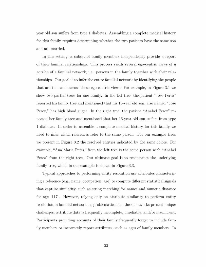
year old son suffers from type 1 diabetes. Assembling a complete medical history

for this family requires determining whether the two patients have the same son

and are married.

In this setting, a subset of family members independently provide a report

of their familial relationships. This process yields several ego-centric views of a

portion of a familial network, i.e., persons in the family together with their rela-

tionships. Our goal is to infer the entire familial network by identifying the people

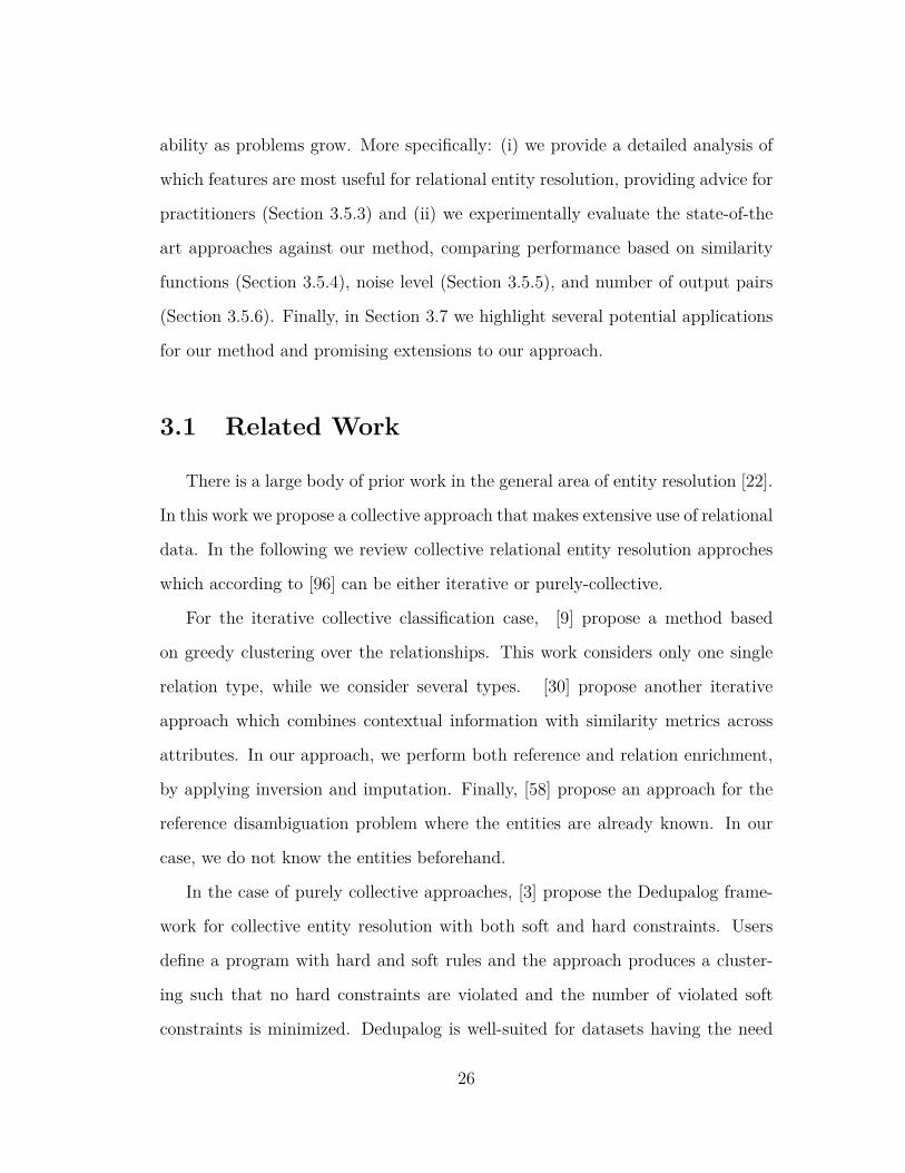
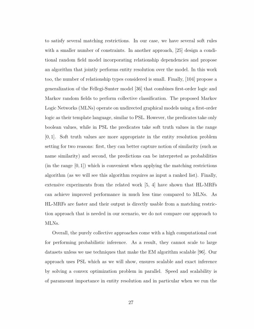
that are the same across these ego-centric views. For example, in Figure 3.1 we

show two partial trees for one family. In the left tree, the patient “Jose Perez”

reported his family tree and mentioned that his 15-year old son, also named “Jose

Perez,” has high blood sugar. In the right tree, the patient “Anabel Perez” re-

ported her family tree and mentioned that her 16-year old son suffers from type

1 diabetes. In order to assemble a complete medical history for this family we

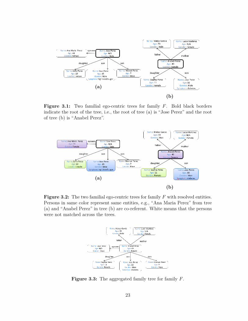
need to infer which references refer to the same person. For our example trees

we present in Figure 3.2 the resolved entities indicated by the same colors. For

example, “Ana Maria Perez” from the left tree is the same person with “Anabel

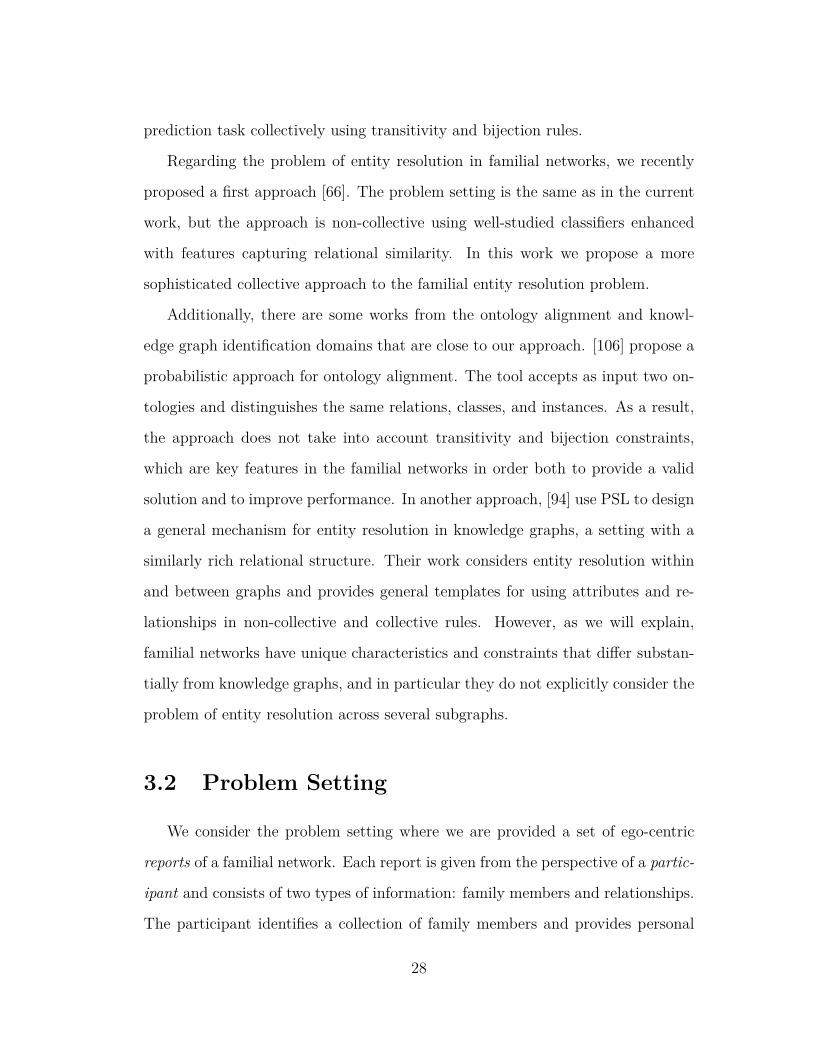
Perez” from the right tree. Our ultimate goal is to reconstruct the underlying

family tree, which in our example is shown in Figure 3.3.

Typical approaches to performing entity resolution use attributes characteriz-

ing a reference (e.g., name, occupation, age) to compute different statistical signals

that capture similarity, such as string matching for names and numeric distance

for age [117]. However, relying only on attribute similarity to perform entity

resolution in familial networks is problematic since these networks present unique

challenges: attribute data is frequently incomplete, unreliable, and/or insufficient.

Participants providing accounts of their family frequently forget to include fam-

ily members or incorrectly report attributes, such as ages of family members. In

22

(a)

(b)

Figure 3.1: Two familial ego-centric trees for family F . Bold black bordersindicate the root of the tree, i.e., the root of tree (a) is “Jose Perez” and the rootof tree (b) is “Anabel Perez”.

(a)

(b)

Figure 3.2: The two familial ego-centric trees for family F with resolved entities.Persons in same color represent same entities, e.g., “Ana Maria Perez” from tree(a) and “Anabel Perez” in tree (b) are co-referent. White means that the personswere not matched across the trees.

Figure 3.3: The aggregated family tree for family F .

23

other cases, they refer to the names using alternate forms. For example, consider

the two ego-centric trees of Figure 3.1. The left tree contains one individual with

the name “Ana Maria Perez” (age 41) and the right one an individual with the

name “Anabel Perez” (age 40). In this case, using name and age similarity only,

we may possibly determine that these persons are not co-referent, since their ages

do not match and the names vary substantially. Furthermore, even when partici-

pants provide complete and accurate attribute information, this information may

be insufficient for entity resolution in familial networks. In the same figure, the

left tree contains two individuals of the name “Jose Perez”, while the right tree

contains only one individual “Jose Perez.” Here, since we have a perfect match for

names for these three individuals, we cannot reach a conclusion which of the two

individuals of the left tree named after “Jose Perez” match the individual “Jose

Perez” from the right tree. Additionally using age similarity would help in the

decision, however, this information is missing for one person. In both cases, the

performance of traditional approaches that rely on attribute similarities suffers in

the setting of familial trees.

In this scenario, there is a clear benefit from exploiting relational informa-

tion in the familial networks. Approaches incorporating relational similarities [9,

30, 58] frequently outperform those relying on attribute-based similarities alone.

Collective approaches [104] where related resolution decisions are made jointly,

rather than independently, showed improved entity resolution performance, albeit

with the tradeoff of increased time complexity. General approaches to collective

entity resolution have been proposed [94], but these are generally appropriate for

one or two networks and do not handle many of the unique challenges of familial

networks. Accordingly, much of the prior work in collective, relational entity res-

olution has incorporated only one, or a handful, of relational types, has limited

24

entity resolution to one or two networks, or has been hampered by scalability

concerns.

In contrast to previous approaches, we develop a scalable approach for collec-

tive relational entity resolution across multiple networks with multiple relationship

types. Our approach is capable of using incomplete and unreliable data in concert

with the rich multi-relational structure found in familial networks. Additionally,

our model can also incorporate input from other algorithms when such informa-

tion is available. We view the problem of entity resolution in familial networks

as a collective classification problem and propose a model that can incorporate

statistical signals, relational information, logical constraints, and predictions from

other algorithms. Our model is able to collectively reason about entities across

networks using these signals, resulting in improved accuracy. To build our model,

we use probabilistic soft logic (PSL) which was described in detail in Chapter 2.

We reiterate that PSL is especially well-suited to entity resolution tasks due to its

ability to unify attributes, relations, constraints such as bijection and transitivity,

and predictions from other models, into a single model.

The remainder of this Chapter is structured as follows. In Section 3.2 we for-

mally define the problem of entity resolution for familial networks . In Section 3.1

we provide a survey of related approaches to relational entity resolution. In Sec-

tion 3.3 we introduce a process of normalization that enables the use of relational

features for entity resolution in familial networks. In Section 3.4 we develop a scal-

able entity resolution framework that effectively combines attributes, relational

information, logical constraints, and predictions from other baseline algorithms.

In Section 3.5 we perform extensive evaluation on two real-world datasets, from

real patient data from the National Institutes of Health and Wikidata, demon-

strating that our approach beats state-of-the-art methods while maintaining scal-

25

ability as problems grow. More specifically: (i) we provide a detailed analysis of

which features are most useful for relational entity resolution, providing advice for

practitioners (Section 3.5.3) and (ii) we experimentally evaluate the state-of-the

art approaches against our method, comparing performance based on similarity

functions (Section 3.5.4), noise level (Section 3.5.5), and number of output pairs

(Section 3.5.6). Finally, in Section 3.7 we highlight several potential applications

for our method and promising extensions to our approach.

3.1 Related Work

There is a large body of prior work in the general area of entity resolution [22].

In this work we propose a collective approach that makes extensive use of relational

data. In the following we review collective relational entity resolution approches

which according to [96] can be either iterative or purely-collective.

For the iterative collective classification case, [9] propose a method based

on greedy clustering over the relationships. This work considers only one single

relation type, while we consider several types. [30] propose another iterative

approach which combines contextual information with similarity metrics across

attributes. In our approach, we perform both reference and relation enrichment,

by applying inversion and imputation. Finally, [58] propose an approach for the

reference disambiguation problem where the entities are already known. In our

case, we do not know the entities beforehand.

In the case of purely collective approaches, [3] propose the Dedupalog frame-

work for collective entity resolution with both soft and hard constraints. Users

define a program with hard and soft rules and the approach produces a cluster-

ing such that no hard constraints are violated and the number of violated soft

constraints is minimized. Dedupalog is well-suited for datasets having the need

26

to satisfy several matching restrictions. In our case, we have several soft rules

with a smaller number of constraints. In another approach, [25] design a condi-

tional random field model incorporating relationship dependencies and propose

an algorithm that jointly performs entity resolution over the model. In this work

too, the number of relationship types considered is small. Finally, [104] propose a

generalization of the Fellegi-Sunter model [36] that combines first-order logic and

Markov random fields to perform collective classification. The proposed Markov

Logic Networks (MLNs) operate on undirected graphical models using a first-order

logic as their template language, similar to PSL. However, the predicates take only

boolean values, while in PSL the predicates take soft truth values in the range

[0, 1]. Soft truth values are more appropriate in the entity resolution problem

setting for two reasons: first, they can better capture notion of similarity (such as

name similarity) and second, the predictions can be interpreted as probabilities

(in the range [0, 1]) which is convenient when applying the matching restrictions

algorithm (as we will see this algorithm requires as input a ranked list). Finally,

extensive experiments from the related work [5, 4] have shown that HL-MRFs

can achieve improved performance in much less time compared to MLNs. As

HL-MRFs are faster and their output is directly usable from a matching restric-

tion approach that is needed in our scenario, we do not compare our approach to

MLNs.

Overall, the purely collective approaches come with a high computational cost

for performing probabilistic inference. As a result, they cannot scale to large

datasets unless we use techniques that make the EM algorithm scalable [96]. Our

approach uses PSL which as we will show, ensures scalable and exact inference

by solving a convex optimization problem in parallel. Speed and scalability is

of paramount importance in entity resolution and in particular when we run the

27

prediction task collectively using transitivity and bijection rules.

Regarding the problem of entity resolution in familial networks, we recently

proposed a first approach [66]. The problem setting is the same as in the current

work, but the approach is non-collective using well-studied classifiers enhanced

with features capturing relational similarity. In this work we propose a more

sophisticated collective approach to the familial entity resolution problem.

Additionally, there are some works from the ontology alignment and knowl-

edge graph identification domains that are close to our approach. [106] propose a

probabilistic approach for ontology alignment. The tool accepts as input two on-

tologies and distinguishes the same relations, classes, and instances. As a result,

the approach does not take into account transitivity and bijection constraints,

which are key features in the familial networks in order both to provide a valid

solution and to improve performance. In another approach, [94] use PSL to design

a general mechanism for entity resolution in knowledge graphs, a setting with a

similarly rich relational structure. Their work considers entity resolution within

and between graphs and provides general templates for using attributes and re-

lationships in non-collective and collective rules. However, as we will explain,

familial networks have unique characteristics and constraints that differ substan-

tially from knowledge graphs, and in particular they do not explicitly consider the

problem of entity resolution across several subgraphs.

3.2 Problem Setting

We consider the problem setting where we are provided a set of ego-centric

reports of a familial network. Each report is given from the perspective of a partic-

ipant and consists of two types of information: family members and relationships.

The participant identifies a collection of family members and provides personal

28

information such as name, age, and gender for each person (including herself).

The participant also reports their relationships to each family member, which we

categorize as first-degree relationships (mother, father, sister, daughter, etc.) or

second-degree relationships (grandfather, aunt, nephew, etc.). Our task is to align

family members across reports in order to reconstruct a complete family tree. We

refer to this task as entity resolution in familial networks and formally define the

problem as follows:

Problem Definition. We assume there is an underlying family F = 〈A,Q〉

which contains (unobserved) actors A and (unobserved) relationships Q amongst

them. We define A = {A1, A2, . . . , Am} and Q = {rta(Ai, Aj), rta(Ai, Ak),

rtb(Ak, Al) . . . rtz (Ak, Am)}. Here ta, tb, tz ∈ τ are different relationship types be-

tween individuals (e.g. son, daughter, father, aunt). Our goal is to recover F from

a set of k participant reports, R.

We define these reports as R = {R1,R2, . . . ,Rk}, where superscripts will

henceforth denote the participant associated with the reported data. Each report,

Ri = 〈pi,Mi,Qi〉 is defined by the reporting participant, pi, the set of family

members mentioned in the report, Mi, and the participant’s relationships to each

mention, Qi. We denote the mentions, Mi = {pi,mi1, . . . ,m

ili}, where each of the

li mentions includes (possibly erroneous) personal attributes and corresponds to a

distinct, unknown actor in the family tree (note that the participant is a mention

as well). We denote the relationships Qi = {rta(pi,mix), . . . , rtb

(pi,miy)}, where

ta, tb ∈ τ denote the types of relation, and mix and mi

y denote the mentioned

family members with whom the participant pi shares the relation types ta and

tb respectively. A participant pi can have an arbitrary number of relations of

the same type (e.g. two daughters, three brothers, zero sisters). Our goal is

to examine all the mentions (participants and non-participants) and perform a

29

matching across reports to create sets of mentions that correspond to the same

actor. The ultimate task is to construct the unified family F from the collection

of matches.

Entity Resolution Task. A prevalent approach to entity resolution is to cast

the problem as a binary, supervised classification task and use machine learn-

ing to label each pair of entities as matching or non-matching. In our specific

problem setting, this corresponds to introducing a variable Same(x, y) for each

pair of entities x, y occurring in distinct participant reports. Formally, we de-

fine the variable Same(mix,m

jy) for each pair of mentions in distinct reports, i.e.,

∀i 6=j∀mix∈Mi∀mj

y∈Mj . Our goal is to determine for each pair of mentions if they

refer to the same actor.

In order to achieve this goal, we must learn a decision function that, given

two mentions, determines if they are the same. Although the general problem

of entity resolution is well-studied, we observe that a significant opportunity in

this specific problem setting is the ability to leverage the familial relationships

in each report to perform relational entity resolution. Unfortunately, the avail-

able reports, R are each provided from the perspective of a unique participant.

This poses a problem since we require relational information for each mention in

a report, not just for the reporting participant. As a concrete example, if one

participant report mentions a son and another report mentions a brother, com-

paring these mentions from the perspectives of a parent and sibling, respectively,

is complex. Instead, if relational features of the mention could be reinterpreted

from a common perspective, the two mentions could be compared directly. We

refer to the problem of recovering mention-specific relational features from partic-

ipant reports as relational normalization, and present our algorithm in the next

section.

30

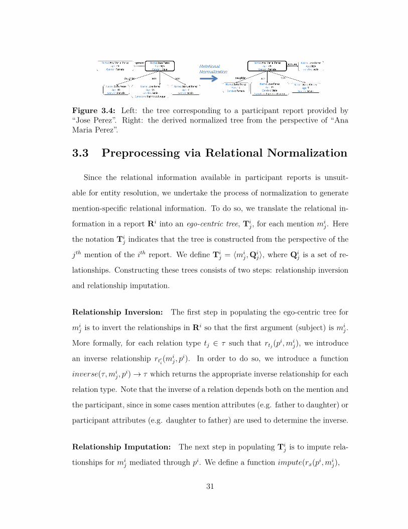
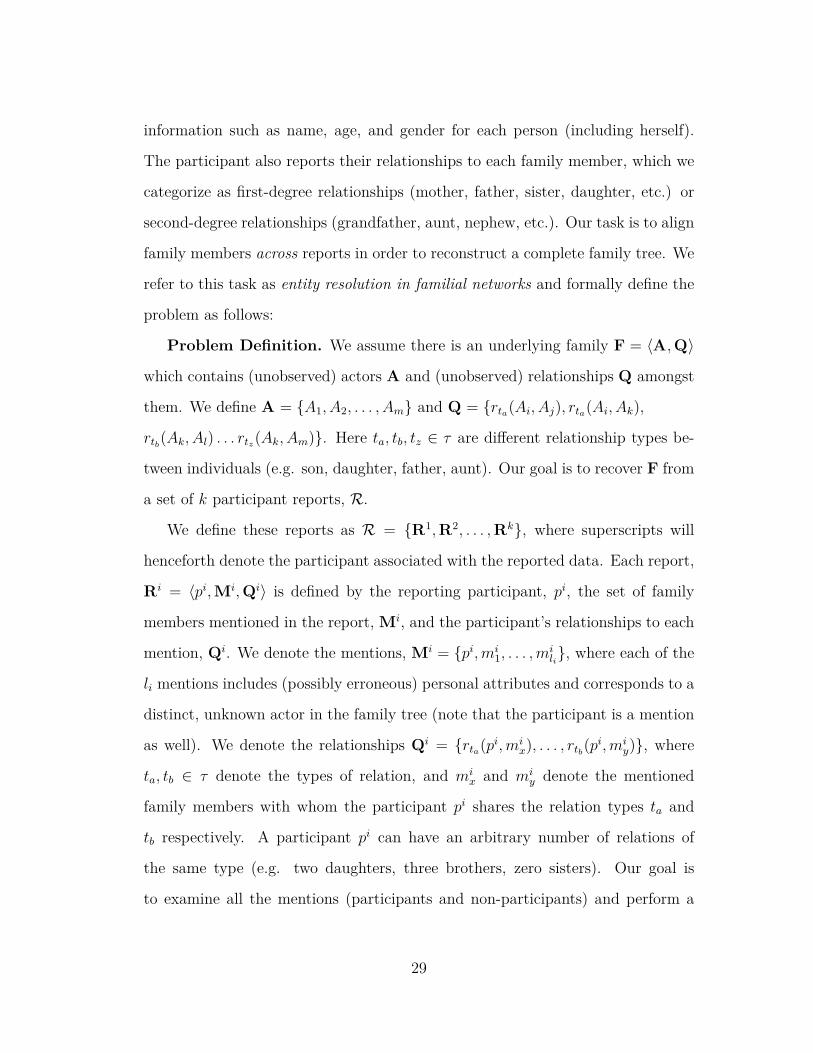
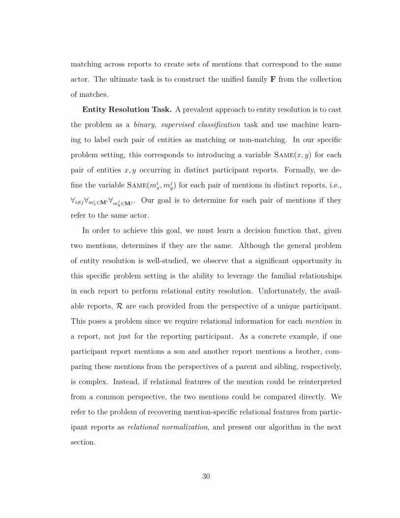
Figure 3.4: Left: the tree corresponding to a participant report provided by“Jose Perez”. Right: the derived normalized tree from the perspective of “AnaMaria Perez”.

3.3 Preprocessing via Relational Normalization

Since the relational information available in participant reports is unsuit-

able for entity resolution, we undertake the process of normalization to generate

mention-specific relational information. To do so, we translate the relational in-

formation in a report Ri into an ego-centric tree, Tij, for each mention mi

j. Here

the notation Tij indicates that the tree is constructed from the perspective of the

jth mention of the ith report. We define Tij = 〈mi

j,Qij〉, where Qi

j is a set of re-

lationships. Constructing these trees consists of two steps: relationship inversion

and relationship imputation.

Relationship Inversion: The first step in populating the ego-centric tree for

mij is to invert the relationships in Ri so that the first argument (subject) is mi

j.

More formally, for each relation type tj ∈ τ such that rtj(pi,mi

j), we introduce

an inverse relationship rt′i(mi

j, pi). In order to do so, we introduce a function

inverse(τ,mij, p

i)→ τ which returns the appropriate inverse relationship for each

relation type. Note that the inverse of a relation depends both on the mention and

the participant, since in some cases mention attributes (e.g. father to daughter) or

participant attributes (e.g. daughter to father) are used to determine the inverse.

Relationship Imputation: The next step in populating Tij is to impute rela-

tionships for mij mediated through pi. We define a function impute(rx(pi,mi

j),

31

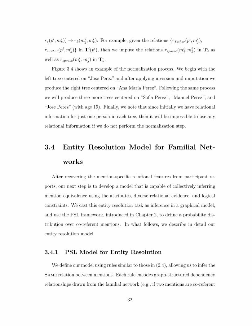
ry(pi,mik))→ rk(mi

j,mik). For example, given the relations {rfather(pi,mi

j),

rmother(pi,mik)} in Ti(pi), then we impute the relations rspouse(mi

j,mik) in Ti

j as

well as rspouse(mik,m

ij) in Ti

k.

Figure 3.4 shows an example of the normalization process. We begin with the

left tree centered on “Jose Perez” and after applying inversion and imputation we

produce the right tree centered on “Ana Maria Perez”. Following the same process

we will produce three more trees centered on “Sofia Perez”, “Manuel Perez”, and

“Jose Perez” (with age 15). Finally, we note that since initially we have relational

information for just one person in each tree, then it will be impossible to use any

relational information if we do not perform the normalization step.

3.4 Entity Resolution Model for Familial Net-

works

After recovering the mention-specific relational features from participant re-

ports, our next step is to develop a model that is capable of collectively inferring

mention equivalence using the attributes, diverse relational evidence, and logical

constraints. We cast this entity resolution task as inference in a graphical model,

and use the PSL framework, introduced in Chapter 2, to define a probability dis-

tribution over co-referent mentions. In what follows, we describe in detail our

entity resolution model.

3.4.1 PSL Model for Entity Resolution

We define our model using rules similar to those in (2.4), allowing us to infer the

Same relation between mentions. Each rule encodes graph-structured dependency

relationships drawn from the familial network (e.g., if two mentions are co-referent

32

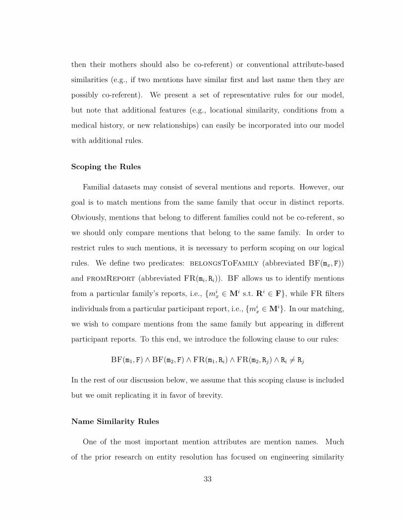
then their mothers should also be co-referent) or conventional attribute-based

similarities (e.g., if two mentions have similar first and last name then they are

possibly co-referent). We present a set of representative rules for our model,

but note that additional features (e.g., locational similarity, conditions from a

medical history, or new relationships) can easily be incorporated into our model

with additional rules.

Scoping the Rules

Familial datasets may consist of several mentions and reports. However, our

goal is to match mentions from the same family that occur in distinct reports.

Obviously, mentions that belong to different families could not be co-referent, so

we should only compare mentions that belong to the same family. In order to

restrict rules to such mentions, it is necessary to perform scoping on our logical

rules. We define two predicates: belongsToFamily (abbreviated BF(mx, F))

and fromReport (abbreviated FR(mi, Ri)). BF allows us to identify mentions

from a particular family’s reports, i.e., {mix ∈ Mi s.t. Ri ∈ F}, while FR filters

individuals from a particular participant report, i.e., {mix ∈Mi}. In our matching,

we wish to compare mentions from the same family but appearing in different

participant reports. To this end, we introduce the following clause to our rules:

BF(m1, F) ∧BF(m2, F) ∧ FR(m1, Ri) ∧ FR(m2, Rj) ∧ Ri 6= Rj

In the rest of our discussion below, we assume that this scoping clause is included

but we omit replicating it in favor of brevity.

Name Similarity Rules

One of the most important mention attributes are mention names. Much

of the prior research on entity resolution has focused on engineering similarity

33

functions that can accurately capture patterns in name similarity. Two such pop-

ular similarity functions are the Levenshtein [81] and Jaro-Winkler [117]. The

first is known to work well for common typographical errors, while the second is

specifically designed to work well with names. We leverage mention names by

introducing rules that capture the intuition that when two mentions have simi-

lar names then they are more likely to represent the same person. For example,

when using the Jaro-Winkler function to compute the name similarities, we use

the following rule:

SimNameJW (m1, m2)⇒ Same(m1, m2) .

This rule reinforces an important aspect of PSL: atoms take truth values in the

[0, 1] interval, capturing the degree of certainty of the inference. In the above rule,

high name similarity results in greater confidence that two mentions are the same.

However, we also wish to penalize pairs of mentions with dissimilar names from

matching, for which we introduce the rule using the logical not (¬):

¬SimNameJW (m1, m2)⇒ ¬Same(m1, m2) .

The above rules use a generic SimName similarity function. In fact, our model

introduces several name similarities for first, last, and middle names as follows:

SimFirstNameJW (m1, m2)⇒ Same(m1, m2)

SimMaidenNameJW (m1, m2)⇒ Same(m1, m2)

SimLastNameJW (m1, m2)⇒ Same(m1, m2)

¬SimFirstNameJW (m1, m2)⇒ ¬Same(m1, m2)

¬SimMaidenNameJW (m1, m2)⇒ ¬Same(m1, m2)

¬SimLastNameJW (m1, m2)⇒ ¬Same(m1, m2) .

In the above rules we use the Jaro-Winkler similarity function. In our basic

34

model, we additionally introduce the same rules that compute similarities using

the Levenshtein distance as well. Finally, we experiment with adding other pop-

ular similarity functions, i.e., Monge Elkan, Soundex, Jaro [117], and their com-

binations and discuss how different string similarity metrics affect performance in

the experimental section.

Personal Information Similarity Rules

In addition to the name attributes of a mention, there are often additional

attributes provided in reports that are useful for matching. For example, age

is an important feature for entity resolution in family trees since it can help us

discern between individuals having the same (or very similar) name but belonging

to different generations. We introduce the following rules for age:

SimAge(m1, m2)⇒ Same(m1, m2)

¬SimAge(m1, m2)⇒ ¬Same(m1, m2) .(3.1)

The predicate SimAge(m1, m2) takes values in the interval [0, 1] and is com-

puted as the ratio of the smallest over the largest value, i.e.:

SimAge(m1, m2) = min{m1.age, m2.age}max{m1.age, m2.age}

.

The above rules will work well when the age is known. However, in the familial

networks setting that we are operating on it is often the case where personal

information and usually the age is not known. For these cases, we can specifically

ask from our model to take into account only cases where the personal information

is known and ignore it when this is not available. To this end, we replace the rules

in (3.1) with the following:

35

KnownAge(m1) ∧KnownAge(m2) ∧ SimAge(m1, m2)⇒ Same(m1, m2)

KnownAge(m1) ∧KnownAge(m2) ∧ ¬SimAge(m1, m2)⇒ ¬Same(m1, m2)

In other words, using the scoping predicates KnownAge(m1) and

KnownAge(m2) we can handle missing values in the PSL model, which is an

important characteristic.

While attributes like age have influence in matching, other attributes cannot

be reliably considered as evidence to matching but they are far more important

in disallowing matches between the mentions. For example, simply having the

same gender is not a good indicator that two mentions are co-referent. However,

having a different gender is a strong evidence that two mentions are not co-referent.

To this end, we also introduce rules that prevent mentions from matching when

certain attributes differ:

¬eqGender(m1, m2)⇒ ¬Same(m1, m2)

¬eqLiving(m1, m2)⇒ ¬Same(m1, m2) .

We note that the predicates eqGender(m1, m2) and eqLiving(m1, m2) are binary-

valued atoms.

Relational Similarity Rules

Although attribute similarities provide useful features for entity resolution, in

problem settings such as familial networks, relational features are necessary for

matching. Relational features can be introduced in a multitude of ways. One

possibility is to incorporate purely structural features, such as the number and

types of relationships for each mention. For example, given a mention with two

sisters and three sons and a mention with three sisters and three sons, we could

design a similarity function for these relations. However, practically this approach

36

lacks discriminative power because there are often mentions that have similar

relational structures (e.g., having a mother) that refer to different entities. To

overcome the lack of discriminative power, we augment structural similarity with

a matching process. For relationship types that are surjective, such as mother or

father, the matching process is straightforward. We introduce a rule:

SimMother(m1, m2)⇒ Same(m1, m2) ,

SimMother may have many possible definitions, ranging from an exact string

match to a recursive similarity computation. In this subsection, we define SimMother

as equal to the maximum of the Levenshtein and Jaro-Winkler similarities of

the first names, and discuss a more sophisticated treatment in the next sub-

section. However, when a relationship type is multi-valued, such as sister or

son, a more sophisticated matching of the target individuals is required. Given

a relation type t and possibly co-referent mentions mi1,m

j2, we find all entities

Mx = {mix : rt(mi

1,mix) ∈ Qi

1} and My = {mjy : rt(mj

2,mjy) ∈ Qj

2}. Now we must

define a similarity for the sets Mx and My, which in turn will provide a similarity

for mi1 and mj

2. The similarity function we use is:

Simt(m1, m2) = 1|Mx|

∑mx∈Mx

maxmy∈My

SimName(mx, my) .

For each mx (an individual with relation t to m1), this computation greedily chooses

the best my (an individual with relation t to m2). In our computation, we assume

(without loss of generality, assuming symmetry of the similarity function) that

|Mx| < |My|. While many possible similarity functions can be used for SimName,

we take the maximum of the Levenshtein and Jaro-Winkler similarities of the first

names in our model.

Our main goal in introducing these relational similarities is to incorporate

relational evidence that is compatible with simpler, baseline models. While more

37

sophisticated than simple structural matches, these relational similarities are much

less powerful than the transitive relational similarities supported by PSL, which

we introduce in the next section.

Transitive Relational (Similarity) Rules

The rules that we have investigated so far can capture personal and relational

similarities but they cannot identify similar persons in a collective way. To make

this point clear, consider the following observation: when we have high confidence

that two persons are the same, we also have a stronger evidence that their associ-

ated relatives, e.g., father, are also the same. We encode this intuition with rules

of the following type:

Rel(Father, m1, ma) ∧Rel(Father, m2, mb) ∧ Same(m1, m2)⇒ Same(ma, mb) .

The rule above works well with surjective relationships, since each person can

have only one (biological) father. When the cardinality is larger, e.g., sister, our

model must avoid inferring that all sisters of two respective mentions are the

same. In these cases we use additional evidence, i.e., name similarity, to select

the appropriate sisters to match, as follows:

Rel(Sister, m1, ma) ∧ Rel(Sister, m2, mb) ∧ Same(m1, m2) ∧ SimName(ma, mb)

⇒ Same(ma, mb) .

Just as in the previous section, we compute SimName by using the maximum of

the Jaro-Winkler and Levenshtein similarities for first names. For relationships

that are one-to-one we can also introduce negative rules which express the intuition

that two different persons should be connected to different persons given a specific

relationship. For example, for a relationship such as spouse, we can use a rule

38

such as:

Rel(Spouse, m1, ma) ∧Rel(Spouse, m2, mb) ∧ ¬Same(m1, m2)⇒ ¬Same(ma, mb) .

However, introducing similar rules for one-to-many relationships is inadvisable.

To understand why, consider the case where two siblings do not match, yet they

have the same mother, whose match confidence should remain unaffected.

Bijection and Transitivity Rules

Our entity resolution task has several natural constraints across reports. The

first is bijection, namely that a mention mix can match at most one mention, mj

y

from another report. According to the bijection rule, if mention ma from report

R1 is matched to mention mb from report R2 then m1 cannot be matched to any

other mention from report R2:

FR(ma, R1) ∧ FR(mb, R2) ∧ FR(mc, R2) ∧ Same(ma, mb)⇒ ¬Same(ma, mc) .

Note that this bijection is soft, and does not guarantee a single, exclusive match for

ma, but rather attenuates the confidence in each possible match modulated by the

evidence for the respective matches. A second natural constraint is transitivity,

which requires that if mia and mj

y are the same, and mentions mjy and mk

c are

the same, then mentions mia and mk

c should also be the same. We capture this

constraint as follows:

FR(ma, R1) ∧ FR(mb, R2) ∧ FR(mc, R3) ∧ Same(ma, mb) ∧ Same(mb, mc)⇒

Same(ma, mc) .

Prior Rule

Entity resolution is typically an imbalanced classification problem, meaning

that most of the mention pairs are not co-referent. We can model our general

39

belief that two mentions are likely not co-referent, using the prior rule:

¬Same(m1, m2) .

Rules to Leverage Existing Classification Algorithms

Every state-of-the-art classification algorithm has strengths and weaknesses

which may depend on data-specific factors such as the degree of noise in the

dataset. In this work, our goal is to provide a flexible framework that can be used

to generate accurate entity resolution decisions for any data setting. To this end,

we can also incorporate the predictions from different methods into our unified

model. Using PSL as a meta-model has been successfully applied in recent work

[92]. In our specific scenario of entity resolution, for example, the predictions

from three popular classifiers (logistic regression (LR), support vector machines

(SVMs), and logistic model trees (LMTs)) can be incorporated in the model via

the following rules:

SameLR(m1, m2)⇒ Same(m1, m2)

¬SameLR(m1, m2)⇒ ¬Same(m1, m2)

SameSVMs(m1, m2)⇒ Same(m1, m2)

¬SameSVMs(m1, m2)⇒ ¬Same(m1, m2)

SameLMTs(m1, m2)⇒ Same(m1, m2)

¬SameLMTs(m1, m2)⇒ ¬Same(m1, m2) .

Note that for each classifier we introduce two rules: 1) the direct rule which

states that if a given classifier predicts that the mentions are co-referent then it

is likely that they are indeed co-referent and 2) the reverse rule which states that

if the classifier predicts that the mentions are not co-referent then it is likely that

40

they are not co-referent. Additionally, using PSL we can introduce more complex

rules that combine the predictions from the other algorithms. For example, if all

three classifiers agree that a pair of mentions are co-referent then this is strong

evidence that this pair of mentions are indeed co-referent. Similarly, if all three

classifiers agree that the pair of mentions are not co-referent then this is strong

evidence that they are not co-referent. We can model these ideas through the

following rules:

SameLR(m1, m2) ∧ SameSVMs(m1, m2) ∧ SameLMTs(m1, m2)⇒

Same(m1, m2)

¬SameLR(m1, m2) ∧ ¬SameSVMs(m1, m2) ∧ ¬SameLMTs(m1, m2)⇒

¬Same(m1, m2) .

Flexible Modeling

We reiterate that in this section we have only provided representative rules

used in our PSL model for entity resolution. A full compendium of all rules

used in our experiments is presented in Appendix 6.1. Moreover, a key feature

of our model is the flexibility and the ease with which it can be extended to

incorporate new features. For example, adding additional attributes, such as

profession or location, is easy to accomplish following the patterns of Subsection

3.4.1. Incorporating additional relationships, such as cousins or friends is simply

accomplished using the patterns in Subsections 3.4.1 and 3.4.1. Our goal has been

to present a variety of patterns that are adaptable across different datasets and

use cases.

41

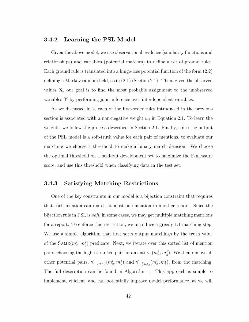
3.4.2 Learning the PSL Model

Given the above model, we use observational evidence (similarity functions and

relationships) and variables (potential matches) to define a set of ground rules.

Each ground rule is translated into a hinge-loss potential function of the form (2.2)

defining a Markov random field, as in (2.1) (Section 2.1). Then, given the observed

values X, our goal is to find the most probable assignment to the unobserved

variables Y by performing joint inference over interdependent variables.

As we discussed in 2, each of the first-order rules introduced in the previous

section is associated with a non-negative weight wj in Equation 2.1. To learn the

weights, we follow the process described in Section 2.1. Finally, since the output

of the PSL model is a soft-truth value for each pair of mentions, to evaluate our

matching we choose a threshold to make a binary match decision. We choose

the optimal threshold on a held-out development set to maximize the F-measure

score, and use this threshold when classifying data in the test set.

3.4.3 Satisfying Matching Restrictions

One of the key constraints in our model is a bijection constraint that requires

that each mention can match at most one mention in another report. Since the

bijection rule in PSL is soft, in some cases, we may get multiple matching mentions

for a report. To enforce this restriction, we introduce a greedy 1:1 matching step.

We use a simple algorithm that first sorts output matchings by the truth value

of the Same(mix,m

jy) predicate. Next, we iterate over this sorted list of mention

pairs, choosing the highest ranked pair for an entity, (mix,m

jy). We then remove all

other potential pairs, ∀mia,a6=x(mi

a,mjy) and ∀mj

b,b 6=y(mi

x,mjb), from the matching.

The full description can be found in Algorithm 1. This approach is simple to

implement, efficient, and can potentially improve model performance, as we will

42

input : A set of mention pairs classified as MATCH together with thelikelihood of the MATCH

output: A set of mention pairs satisfying the one-to-one matching restrictions1 repeat2 pick unmarked pair {ai, aj} with highest MATCH likelihood;3 output pair {ai, aj} as MATCH;4 mark pair {ai, aj};5 output all other pairs containing either ai or aj as NO MATCH;6 mark all other pairs containing either ai or aj ;7 until all pairs are marked;

Algorithm 1: Satisfying matching restrictions.

discuss in our experiments.

3.5 Experimental Validation

3.5.1 Datasets and Baselines

For our experimental evaluation we use two datasets, a clinical dataset pro-

vided by the National Institutes of Health (NIH) [44] and a public dataset crawled

from the structured knowledge repository, Wikidata.1 We provide summary statis-

tics for both datasets in Table 3.1.

The NIH dataset was collected by interviewing 497 patients from 162 families

and recording family medical histories. For each family, 3 or 4 patients were inter-

viewed, and each interview yielded a corresponding ego-centric view of the family

tree. Patients provided first and second degree relations, such as parents and

grandparents. In total, the classification task requires determining co-reference

for about 300, 000 pairs of mentions. The provided dataset was manually anno-

tated by at least two coders, with differences reconciled by blind consensus. Only

1.6% of the potential pairs are co-referent, resulting in a severely imbalanced1Code and data available at: https://github.com/pkouki/icdm2017.

43

Dataset NIH WikidataNo. of families 162 419No. of family trees 497 1,844No. of mentions 12,111 8,553No. of 1st degree relationships 46,983 49,620No. of 2nd degree relationships 67,540 0No. of pairs for comparison 300,547 174,601% of co-referent pairs 1.6% 8.69%

Table 3.1: Datasets description

classification, which is common in entity resolution scenarios.

The Wikidata dataset was generated by crawling part of the Wikidata2 knowl-

edge base. More specifically, we generated a seed set of 419 well-known politicians

or celebrities, e.g., “Barack Obama”.3 For each person in the seed set, we retrieved

attributes from Wikidata including their full name (and common variants), age,

gender, and living status. Wikidata provides familial data only for first-degree

relationships, i.e., siblings, parents, children, and spouses. Using the available re-

lationships, we also crawled Wikidata to acquire attributes and relationships for

each listed relative. This process resulted in 419 families. For each family, we have

a different number of family trees (ranging from 2 to 18) with 1, 844 family trees

in total, and 175, 000 pairs of potentially co-referent mentions (8.7% of which are

co-referent). Mentions in Wikidata are associated with unique identifiers, which

we use as ground truth. In the next section, we describe how we add noise to this

dataset to evaluate our method.

We compare our approach to state-of-the-art classifiers that are capable of

providing the probability that a given pair of mentions is co-referent. Probability

values are essential since they are the input to the greedy 1-1 matching restrictions

algorithm. We compare our approach to the following classifiers: logistic regres-2https://www.wikidata.org/3https://www.wikidata.org/wiki/Q76

44

sion (LR), logistic model trees (LMTs), and support vector machines (SVMs).

For LR we use a multinomial logistic regression model with a ridge estimator

[18] using the implementation and improvements of Weka [38] with the default

settings. For LMTs we use Weka’s implementation [71] with the default settings.

For SVMs we use Weka’s LibSVM library [19], along with the functionality to

estimate probabilities. To select the best SVM model we follow the process de-

scribed by Hsu et al. [55]: we first find the kernel that performs best, which in our

case was the radial basis function (RBF). We then perform a grid search to find

the best values for C and γ parameters. The starting point for the grid search

was the default values given by Weka, i.e., C=1 and γ=1/(number of attributes),

and we continue the search with exponentially increasing/decreasing sequences of

C and γ. However, unlike our model, none of these off-the-shelf classifiers can

incorporate transitivity or bijection.

Finally, we note that we also experimented with off-the-shelf collective clas-

sifiers provided by Weka.4 More specifically, we experimented with Chopper,

TwoStageCollective, and YATSI [32]. Among those, YATSI performed the best.

YATSI (Yet Another Two-Stage Classifier) is collective in the sense that the pre-

dicted label of a test instance will be influenced by the labels of related test

instances. We experimented with different configurations of YATSI, such as vary-

ing the classification method used, varying the nearest neighbor approach, varying

the number of the neighbors to consider, and varying the weighting factor. In our

experiments, YATSI was not able to outperform the strongest baseline (which as

we will show is LMTs), so, for clarity, we omit these results from our discussion

below.4Available at: https://github.com/fracpete/collective-classification-weka-package

45

3.5.2 Experimental Setup

We evaluate our entity resolution approach using the metrics of precision, re-

call, and F-measure for the positive (co-referent) class which are typical for entity

resolution problems [22]. For all reported results we use 5-fold cross-validation,

with distinct training, development, and test sets. Folds are generated by ran-

domly assigning each of the 162 (NIH) and 419 (Wikidata) families to one of five

partitions, yielding folds that contain the participant reports for approximately

32 (NIH) and 83 (Wikidata) familial networks.

The NIH dataset is collected in a real-world setting where information is nat-

urally incomplete and erroneous, and attributes alone are insufficient to resolve

the entities. However, the Wikidata resource is heavily curated and assumed to

contain no noise. To simulate the noisy conditions of real-world datasets, we in-

troduced additive Gaussian noise to the similarity scores. Noise was added to each

similarity metric described in the previous section (e.g., first name Jaro-Winkler,

age ratio). For the basic experiments presented in the next Section 3.5.3, results

are reported for noise terms drawn from a N(0, 0.16) distribution. In our full ex-

periments (presented in Section 3.5.5) we consider varying levels of noise, finding

higher noise correlated with lower performance.

In Section 3.4.1 we discussed that PSL can incorporate multiple similarities

computed by different string similarity functions. For the basic experiments pre-

sented in the next Section 3.5.3, results are reported using the Levenshtein and

Jaro-Winkler string similarity functions for PSL and the baselines. In our full ex-

periments (presented in Section 3.5.5) we consider adding other string similarity

functions.

In each experiment, for PSL, we use three folds for training the model weights,

one fold for choosing a binary classification threshold, and one fold for evaluating

46

model performance. To train the weights, we use PSL’s default values for the

two parameters: number of iterations (equal to 25) and step size (equal to 1).

For SVMs, we use three folds for training the SVMs with the different values of

C and γ, one fold for choosing the best C and γ combination, and one fold for

evaluating model performance. For LR and LMTs we use three folds for training

the models with the default parameter settings and one fold for evaluating the

models. We train, validate, and evaluate using the same splits for all models. We

report the average precision, recall, and F-measure together with the standard

deviation across folds.

3.5.3 Performance of PSL and baselines

For our PSL model, we start with a simple feature set using only name simi-

larities (see Subsection 3.4.1), transitivity and bijection soft constraints (see Sub-

section 3.4.1), and a prior (see Subsection 3.4.1). We progressively enhance the

model by adding attribute similarities computed based on personal information,

relational similarities, and transitive relationships. For each experiment we ad-

ditionally report results when including predictions from the other baselines (de-

scribed in Subsection 4.3.1). Finally, since our dataset poses the constraint that

each person from one report can be matched with at most one person from an-

other report, we consider only solutions that satisfy this constraint. To ensure

that the output is a valid solution, we apply the greedy 1:1 matching restriction

algorithm (see Subsection 3.4.3) on the output of the each model.

For each of the experiments we also ran baseline models that use the same

information as the PSL models in the form of features. Unlike our models im-

plemented within PSL, the models from the baseline classifiers do not support

collective reasoning, i.e., applying transitivity and bijection is not possible in the

47

baseline models. However, we are able to apply the greedy 1:1 matching restric-

tion algorithm on the output of each of the classifiers for each of the experiments

to ensure that we provide a valid solution. More specifically, we ran the following

experiments:

Names: We ran two PSL models that use as features the first, middle, and

last name similarities based on Levenshtein and Jaro-Winkler functions to com-

pute string similarities. In the first model, PSL(N), we use rules only on name

similarities, as discussed in Section 3.4.1. In the second model, PSL(N + pred)

we enhance PSL(N) by adding rules that incorporate the predictions from the

other baseline models as described in Subsection 4.3.1. We also ran LR, LMTs,

and SVMs models that use as features the first, middle, and last name similarities

based on Levenshtein and Jaro-Winkler measures.

Names + Personal Info: We enhance Names by adding rules about personal

information similarities, as discussed in Section 3.4.1. Again, for PSL we ran

two models: PSL(P ) which does not include predictions from the baselines and

PSL(P + pred) that does include predictions from the baselines. For the base-

lines, we add corresponding features for age similarity, gender, and living status.

This is the most complex feature set that can be supported without using the

normalization procedure we introduced in Section 3.3.

Names + Personal + Relational Info (1st degree): For this model and

all subsequent models we perform normalization to enable the use of relational

evidence for entity resolution. We present the performance of four PSL models.

In the first model, PSL(R1), we enhance PSL(P ) by adding first degree rela-

tional similarity rules, as discussed in Section 3.4.1. First degree relationships

are: mother, father, daughter, son, brother, sister, spouse. In the second model,

48

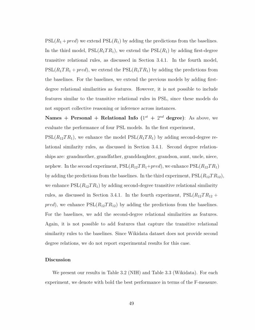
PSL(R1 +pred) we extend PSL(R1) by adding the predictions from the baselines.

In the third model, PSL(R1TR1), we extend the PSL(R1) by adding first-degree

transitive relational rules, as discussed in Section 3.4.1. In the fourth model,

PSL(R1TR1 + pred), we extend the PSL(R1TR1) by adding the predictions from

the baselines. For the baselines, we extend the previous models by adding first-

degree relational similarities as features. However, it is not possible to include

features similar to the transitive relational rules in PSL, since these models do

not support collective reasoning or inference across instances.

Names + Personal + Relational Info (1st + 2nd degree): As above, we

evaluate the performance of four PSL models. In the first experiment,

PSL(R12TR1), we enhance the model PSL(R1TR1) by adding second-degree re-

lational similarity rules, as discussed in Section 3.4.1. Second degree relation-

ships are: grandmother, grandfather, granddaughter, grandson, aunt, uncle, niece,

nephew. In the second experiment, PSL(R12TR1+pred), we enhance PSL(R12TR1)

by adding the predictions from the baselines. In the third experiment, PSL(R12TR12),

we enhance PSL(R12TR1) by adding second-degree transitive relational similarity

rules, as discussed in Section 3.4.1. In the fourth experiment, PSL(R12TR12 +

pred), we enhance PSL(R12TR12) by adding the predictions from the baselines.

For the baselines, we add the second-degree relational similarities as features.

Again, it is not possible to add features that capture the transitive relational

similarity rules to the baselines. Since Wikidata dataset does not provide second

degree relations, we do not report experimental results for this case.

Discussion

We present our results in Table 3.2 (NIH) and Table 3.3 (Wikidata). For each

experiment, we denote with bold the best performance in terms of the F-measure.

49

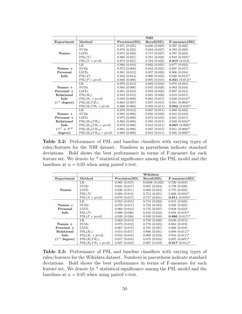
NIHExperiment Method Precision(SD) Recall(SD) F-measure(SD)

LR 0.871 (0.025) 0.686 (0.028) 0.767 (0.022)SVMs 0.870 (0.022) 0.683 (0.027) 0.765 (0.020)

Names LMTs 0.874 (0.020) 0.717 (0.027) 0.787 (0.022)PSL(N) 0.866 (0.021) 0.761 (0.028) 0.810 (0.023)*PSL(N + pred) 0.873 (0.021) 0.764 (0.022) 0.815 (0.019)LR 0.968 (0.010) 0.802 (0.035) 0.877 (0.024)

Names + SVMs 0.973 (0.008) 0.832 (0.025) 0.897 (0.017)Personal LMTs 0.961 (0.012) 0.857 (0.020) 0.906 (0.016)

Info PSL(P ) 0.942 (0.014) 0.900 (0.022) 0.920 (0.015)*PSL(P + pred) 0.949 (0.008) 0.895 (0.018) 0.921 (0.013)*LR 0.970 (0.012) 0.802 (0.034) 0.878 (0.024)

Names + SVMs 0.983 (0.008) 0.835 (0.026) 0.903 (0.018)Personal + LMTs 0.961 (0.010) 0.859 (0.020) 0.907 (0.014)Relational PSL(R1) 0.943 (0.012) 0.881 (0.030) 0.910 (0.015)

Info PSL(R1 + pred) 0.958 (0.009) 0.885 (0.017) 0.920 (0.013)*(1st degree) PSL(R1T R1) 0.964 (0.007) 0.937 (0.015) 0.951 (0.009)*

PSL(R1T R1 + pred) 0.966 (0.009) 0.939 (0.011) 0.952 (0.010)*LR 0.970 (0.012) 0.807 (0.051) 0.880 (0.032)

Names + SVMs 0.985 (0.006) 0.856 (0.029) 0.916 (0.019)Personal + LMTs 0.975 (0.008) 0.872 (0.016) 0.921 (0.011)Relational PSL(R12T R1) 0.964 (0.008) 0.935 (0.017) 0.949 (0.010)*

Info PSL(R12T R1 + pred) 0.970 (0.008) 0.943 (0.011) 0.957 (0.009)*(1st + 2nd PSL(R12T R12) 0.965 (0.008) 0.937 (0.015) 0.951 (0.009)*

degree) PSL(R12T R12 + pred) 0.969 (0.009) 0.943 (0.011) 0.956 (0.008)*

Table 3.2: Performance of PSL and baseline classifiers with varying types ofrules/features for the NIH dataset. Numbers in parenthesis indicate standarddeviations. Bold shows the best performance in terms of F-measure for eachfeature set. We denote by * statistical significance among the PSL model and thebaselines at α = 0.05 when using paired t-test.

WikidataExperiment Method Precision(SD) Recall(SD) F-measure(SD)

LR 0.905 (0.015) 0.6598 (0.022) 0.720 (0.018)SVMs 0.941 (0.017) 0.607 (0.034) 0.738 (0.026)

Names LMTs 0.926 (0.011) 0.660 (0.034) 0.770 (0.023)PSL(N) 0.868 (0.014) 0.754 (0.031) 0.806 (0.016)*PSL(N + pred) 0.876 (0.017) 0.757 (0.031) 0.811 (0.016)*LR 0.953 (0.015) 0.713 (0.032) 0.815 (0.022)

Names + SVMs 0.970 (0.011) 0.723 (0.034) 0.828 (0.023)Personal LMTs 0.960 (0.014) 0.745 (0.037) 0.838 (0.022)

Info PSL(P ) 0.908 (0.026) 0.816 (0.042) 0.858 (0.016)*PSL(P + pred) 0.928 (0.026) 0.839 (0.040) 0.880 (0.017)*LR 0.962 (0.013) 0.756 (0.028) 0.846 (0.015)

Names + SVMs 0.975 (0.012) 0.776 (0.035) 0.864 (0.019)Personal + LMTs 0.967 (0.015) 0.785 (0.037) 0.866 (0.019)Relational PSL(R1) 0.914 (0.017) 0.866 (0.031) 0.889 (0.011)*

Info PSL(R1 + pred) 0.934 (0.018) 0.900 (0.023) 0.916 (0.011)*(1st degree) PSL(R1T R1) 0.917 (0.018) 0.878 (0.016) 0.897 (0.007)*

PSL(R1T R1 + pred) 0.927 (0.018) 0.907 (0.019) 0.917 (0.011)*

Table 3.3: Performance of PSL and baseline classifiers with varying types ofrules/features for the Wikidata dataset. Numbers in parenthesis indicate standarddeviations. Bold shows the best performance in terms of F-measure for eachfeature set. We denote by * statistical significance among the PSL model and thebaselines at α = 0.05 when using paired t-test.

50

We present the results for both our method and the baselines and only for the

positive class (co-referent entities). Due to the imbalanced nature of the task, per-

formance on non-matching entities is similar across all approaches, with precision

varying from 99.6% to 99.9%, recall varying from 99.4% to 99.9%, and F-measure

varying from 99.5% to 99.7% for the NIH dataset. For the Wikidata, precision

varies from 98.7% to 99.8%, recall varies from 98.9% to 99.9%, and F-measure

varies from 99.5% to 99.7%. Furthermore, to highlight the most interesting com-

parisons we introduce Figures 3.5, 3.6, and 3.7 as a complement for the complete

tables. The plots in these figures show the F-measure when varying the classifica-

tion method (i.e., baselines and PSL) or the amount of information used for the

classification (e.g., use only names). Figures in blue are for NIH while figures in

orange are for the Wikidata dataset. Next, we summarize some of our insights

from the results of Tables 3.2 and 3.3. For the most interesting comparisons we

additionally refer to Figures 3.5, 3.6, and 3.7.

PSL models universally outperform baselines: In each experiment PSL

outperforms all the baselines using the same feature set. PSL produces a sta-

tistically significant improvement in F-measure as measured by a paired t-test

with α = 0.05. Of the baselines, LMTs perform best in all experiments and will

be used for illustrative comparison. When using name similarities only (Names

models in Tables 3.2 and 3.3) PSL(N) outperforms LMTs by 2.3% and 3.6%

(absolute value) for the NIH and the Wikidata dataset accordingly. When adding

personal information similarities (Names + Personal Info), PSL(NR) outper-

forms LMTs by 1.4% and 2% for the NIH and the Wikidata accordingly. For the

experiment Names + Personal + Relational Info 1st degree, the PSL model

that uses both relational and transitive relational similarity rules, PSL(R1TR1),

outperforms LMTs by 4.4% for the NIH and 3.1% for the Wikidata. Finally, for

51

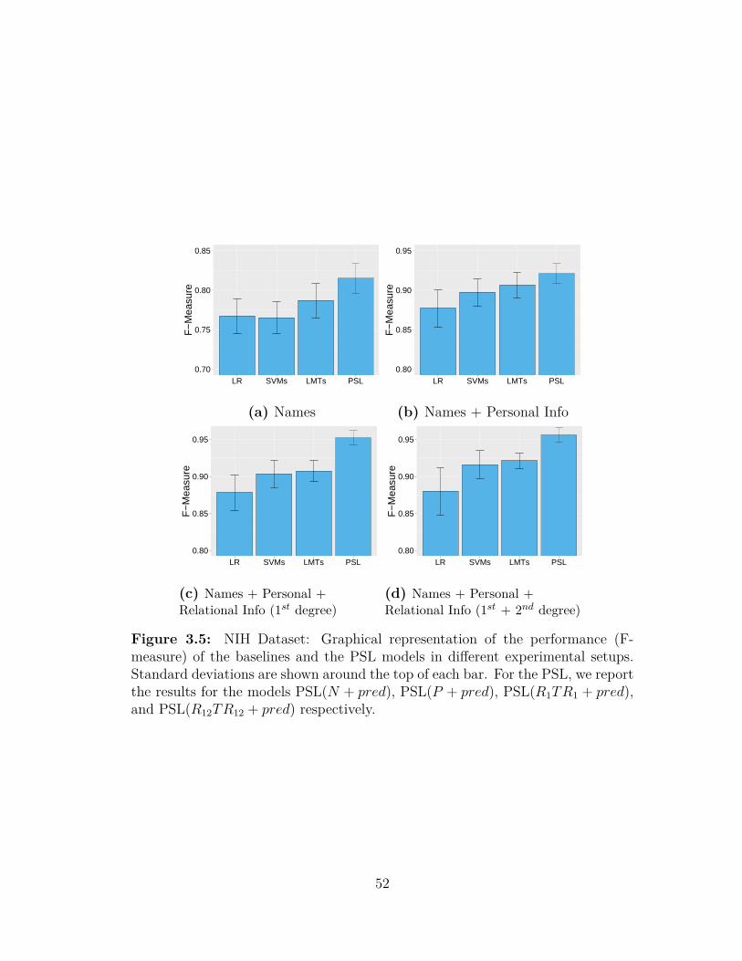
0.70

0.75

0.80

0.85

LR SVMs LMTs PSL

F−

Mea

sure

(a) Names

0.80

0.85

0.90

0.95

LR SVMs LMTs PSLF

−M

easu

re

(b) Names + Personal Info

0.80

0.85

0.90

0.95

LR SVMs LMTs PSL

F−

Mea

sure

(c) Names + Personal +Relational Info (1st degree)

0.80

0.85

0.90

0.95

LR SVMs LMTs PSL

F−

Mea

sure

(d) Names + Personal +Relational Info (1st + 2nd degree)

Figure 3.5: NIH Dataset: Graphical representation of the performance (F-measure) of the baselines and the PSL models in different experimental setups.Standard deviations are shown around the top of each bar. For the PSL, we reportthe results for the models PSL(N + pred), PSL(P + pred), PSL(R1TR1 + pred),and PSL(R12TR12 + pred) respectively.

52

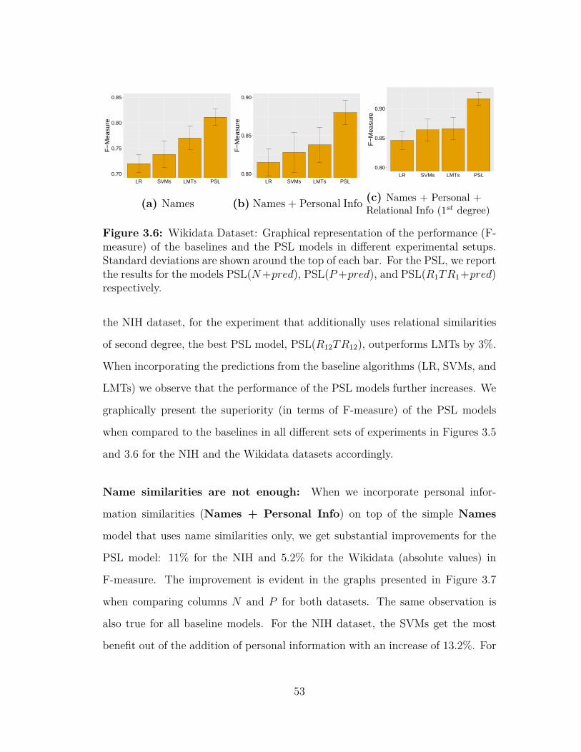
0.70

0.75

0.80

0.85

LR SVMs LMTs PSL

F−

Mea

sure

(a) Names

0.80

0.85

0.90

LR SVMs LMTs PSL

F−

Mea

sure

(b) Names + Personal Info

0.80

0.85

0.90

LR SVMs LMTs PSL

F−

Mea

sure

(c) Names + Personal +Relational Info (1st degree)

Figure 3.6: Wikidata Dataset: Graphical representation of the performance (F-measure) of the baselines and the PSL models in different experimental setups.Standard deviations are shown around the top of each bar. For the PSL, we reportthe results for the models PSL(N+pred), PSL(P+pred), and PSL(R1TR1+pred)respectively.

the NIH dataset, for the experiment that additionally uses relational similarities

of second degree, the best PSL model, PSL(R12TR12), outperforms LMTs by 3%.

When incorporating the predictions from the baseline algorithms (LR, SVMs, and

LMTs) we observe that the performance of the PSL models further increases. We

graphically present the superiority (in terms of F-measure) of the PSL models

when compared to the baselines in all different sets of experiments in Figures 3.5

and 3.6 for the NIH and the Wikidata datasets accordingly.

Name similarities are not enough: When we incorporate personal infor-

mation similarities (Names + Personal Info) on top of the simple Names

model that uses name similarities only, we get substantial improvements for the

PSL model: 11% for the NIH and 5.2% for the Wikidata (absolute values) in

F-measure. The improvement is evident in the graphs presented in Figure 3.7

when comparing columns N and P for both datasets. The same observation is

also true for all baseline models. For the NIH dataset, the SVMs get the most

benefit out of the addition of personal information with an increase of 13.2%. For

53

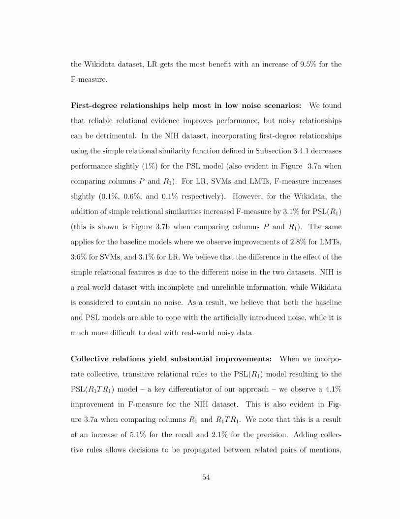
the Wikidata dataset, LR gets the most benefit with an increase of 9.5% for the

F-measure.

First-degree relationships help most in low noise scenarios: We found

that reliable relational evidence improves performance, but noisy relationships

can be detrimental. In the NIH dataset, incorporating first-degree relationships

using the simple relational similarity function defined in Subsection 3.4.1 decreases

performance slightly (1%) for the PSL model (also evident in Figure 3.7a when

comparing columns P and R1). For LR, SVMs and LMTs, F-measure increases

slightly (0.1%, 0.6%, and 0.1% respectively). However, for the Wikidata, the

addition of simple relational similarities increased F-measure by 3.1% for PSL(R1)

(this is shown is Figure 3.7b when comparing columns P and R1). The same

applies for the baseline models where we observe improvements of 2.8% for LMTs,

3.6% for SVMs, and 3.1% for LR. We believe that the difference in the effect of the

simple relational features is due to the different noise in the two datasets. NIH is

a real-world dataset with incomplete and unreliable information, while Wikidata

is considered to contain no noise. As a result, we believe that both the baseline

and PSL models are able to cope with the artificially introduced noise, while it is

much more difficult to deal with real-world noisy data.

Collective relations yield substantial improvements: When we incorpo-

rate collective, transitive relational rules to the PSL(R1) model resulting to the

PSL(R1TR1) model – a key differentiator of our approach – we observe a 4.1%

improvement in F-measure for the NIH dataset. This is also evident in Fig-

ure 3.7a when comparing columns R1 and R1TR1. We note that this is a result

of an increase of 5.1% for the recall and 2.1% for the precision. Adding collec-

tive rules allows decisions to be propagated between related pairs of mentions,

54

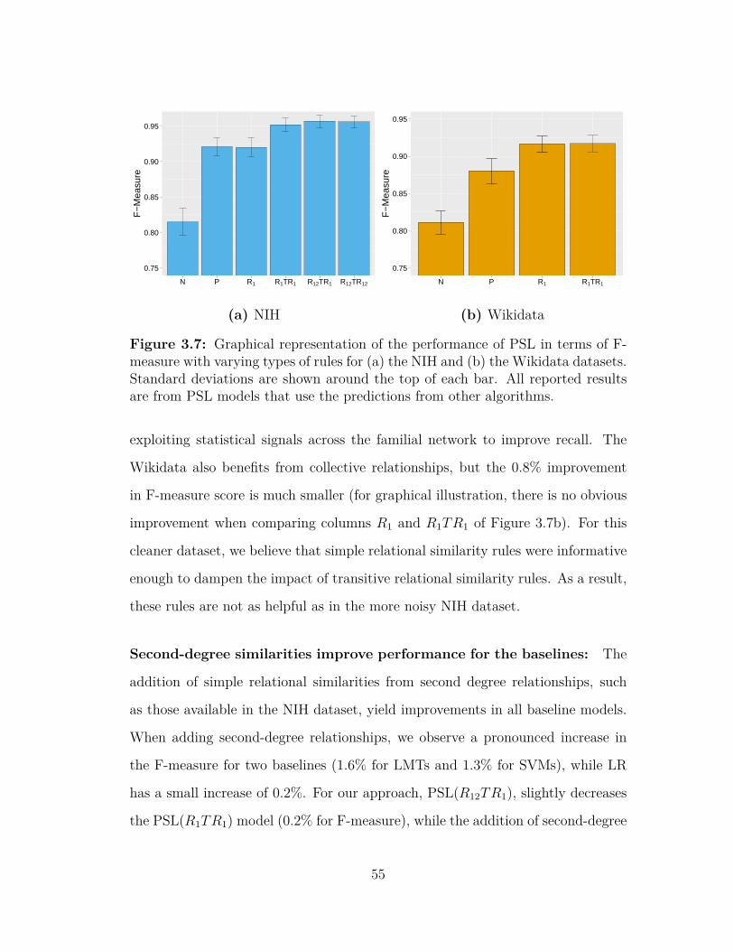
0.75

0.80

0.85

0.90

0.95

N P R1 R1TR1 R12TR1 R12TR12

F−

Mea

sure

(a) NIH

0.75

0.80

0.85

0.90

0.95

N P R1 R1TR1

F−

Mea

sure

(b) Wikidata

Figure 3.7: Graphical representation of the performance of PSL in terms of F-measure with varying types of rules for (a) the NIH and (b) the Wikidata datasets.Standard deviations are shown around the top of each bar. All reported resultsare from PSL models that use the predictions from other algorithms.

exploiting statistical signals across the familial network to improve recall. The

Wikidata also benefits from collective relationships, but the 0.8% improvement

in F-measure score is much smaller (for graphical illustration, there is no obvious

improvement when comparing columns R1 and R1TR1 of Figure 3.7b). For this

cleaner dataset, we believe that simple relational similarity rules were informative

enough to dampen the impact of transitive relational similarity rules. As a result,

these rules are not as helpful as in the more noisy NIH dataset.

Second-degree similarities improve performance for the baselines: The

addition of simple relational similarities from second degree relationships, such

as those available in the NIH dataset, yield improvements in all baseline models.

When adding second-degree relationships, we observe a pronounced increase in

the F-measure for two baselines (1.6% for LMTs and 1.3% for SVMs), while LR

has a small increase of 0.2%. For our approach, PSL(R12TR1), slightly decreases

the PSL(R1TR1) model (0.2% for F-measure), while the addition of second-degree

55

transitive relational features (model PSL(R12TR12)) improves slightly the perfor-

mance by 0.2%.

Predictions from other algorithms always improve performance: In all

our experiments, we ran different versions of the PSL models that included or

omitted the predictions from the baselines, i.e., LR, SVMs, LMTs (discussed in

Subsection 4.3.1). We observe that the addition of the predictions of the other

algorithms always increases the performance of the PSL models. More specifically,

for the NIH dataset, the addition of the predictions from LR, SVMs, and LMTs

slightly increases the F-measure of the PSL models. In particular, F-measure

increases by 0.5% for the experimentNames and 0.1% for the experimentNames

+ Personal Info. Also, the experiment PSL(R1 +pred) improves the F-measure

of the experiment PSL(R1) by 1.0%, and the experiment PSL(R1TR1 + pred)

slightly improves the F-measure of the experiment PSL(R1TR1) by 0.1%. For

the case of the experiment PSL(R1 + pred) we can see that its performance (F-

measure=0.910) is very close to the performance of the baselines (e.g., the F-

measure for the LMTs is 0.907). As a result, adding the baselines helps the PSL

model to better distinguish the true positives and true negatives. However, in

the case of the model PSL(R1TR1) we can see that there is a clear difference

between the PSL model and the baselines, so for this experiment adding the

predictions of those cannot improve at a bigger scale the performance of the PSL

model. Last, for the experiment Names + Personal + Relational Info (1st

+ 2nd degree) we observe that adding the predictions from the other algorithms

slightly increases the F-measure by 0.8% for the experiment PSL(R12TR1 + pred)

and 0.5% for the experiment PSL(R12TR12 + pred). In all cases, we observe that

the increase in F-measure is the result of an increase in both the precision and the

recall of the model (the only case that we observe a small decrease in the recall

56

is the experiment Names + Personal Info). For the Wikidata dataset, we

observe that the F-measure improves significantly in all experiments when adding

the predictions from the baselines. This is a result of the increase of both the

precision and the recall. More specifically, we observe the following increases for

the F-measure: 0.5% for the experimentNames, 2.2% for the experimentNames

+ Personal Info, 2.7% and 2.0% for the two versions of the experiment Names

+ Personal + Relational Info (1st degree).

Precision-recall balance depends on the chosen threshold: As we dis-

cussed in Section 3.4.2 for the PSL model we choose the optimal threshold to

maximize the F-measure score. This learned threshold achieves a precision-recall

balance that favors recall at the expense of precision. For both datasets, our

model’s recall is significantly higher than all the baselines in all the experiments.

However, since PSL outputs soft truth values, changing the threshold selection

criteria in response to the application domain (e.g., prioritizing cleaner matches

over coverage) can allow the model to emphasize precision over recall.

Matching restrictions always improves F-measure: We note that valid

solutions in our entity resolution setting require that an entity matches at most

one entity in another ego-centric network. To enforce this restriction, we apply a

1-1 matching algorithm on the raw output of all models (Section 3.4.3). Applying

matching restrictions adjusts the precision-recall balance of all models. For both

PSL and the baselines across both datasets, when applying the 1-1 matching

restriction algorithm, we observe a sizable increase in precision and a marginal

drop in recall. This pattern matches our expectations, since the algorithm removes

predicted co-references (harming recall) but is expected to primarily remove false-

positive pairs (helping precision). Overall, the application of the 1-1 matching

57

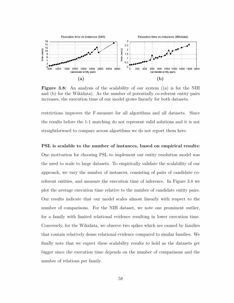
(a) (b)

Figure 3.8: An analysis of the scalability of our system ((a) is for the NIHand (b) for the Wikidata). As the number of potentially co-referent entity pairsincreases, the execution time of our model grows linearly for both datasets.

restrictions improves the F-measure for all algorithms and all datasets. Since

the results before the 1-1 matching do not represent valid solutions and it is not

straightforward to compare across algorithms we do not report them here.

PSL is scalable to the number of instances, based on empirical results:

One motivation for choosing PSL to implement our entity resolution model was

the need to scale to large datasets. To empirically validate the scalability of our

approach, we vary the number of instances, consisting of pairs of candidate co-

referent entities, and measure the execution time of inference. In Figure 3.8 we

plot the average execution time relative to the number of candidate entity pairs.

Our results indicate that our model scales almost linearly with respect to the

number of comparisons. For the NIH dataset, we note one prominent outlier,

for a family with limited relational evidence resulting in lower execution time.

Conversely, for the Wikidata, we observe two spikes which are caused by families

that contain relatively dense relational evidence compared to similar families. We

finally note that we expect these scalability results to hold as the datasets get

bigger since the execution time depends on the number of comparisons and the

number of relations per family.

58

3.5.4 Effect of String Similarity Functions

In Section 3.4.1 we discussed that PSL can easily incorporate a variety of string

similarity functions. In the basic experiments (Section 3.5.3) all models (PSL and

baselines) used the Levensthein and Jaro-Winkler string similarity functions. In

this section, we experiment with a wider set of string similarity functions and

simple combinations of them in order to study how such different functions can

affect performance. More specifically, for all the models (PSL and baselines) we

ran the following experiments:

– Levenshtein (L): We use first, middle, and last name similarities computed

using the Levenshtein string similarity function only.

– Jaro-Winkler (JW ): We add Jaro-Winkler similarities.

– Monge-Elkan (ME): We add Monge-Elkan similarities.

– Soundex (S): We add Soundex similarities.

– Jaro (J): We add Jaro similarities.

– max(L, JW, ME, S, J): We combine the string similarity functions by using

the maximum value of all the similarity functions.

– min(L, JW, ME, S, J): We combine the string similarity functions by using

the minimum value of all the similarity functions.

We note that for the PSL, we run the version PSL(N) and not the version

PSL(N+pred), i.e., we do not use the predictions from the other models in our PSL

model. We present the results in Table 3.4 for the NIH dataset. As we discussed,

for the Wikidata dataset we introduced artificial noise to all the similarities so we

focus on the NIH dataset to get a clear picture of the performance of the similarity

functions. Here is a summary of the results from Table 3.4:

The performance of the models changes when the string similarity

functions change: For PSL, the difference between the model that performs the

59

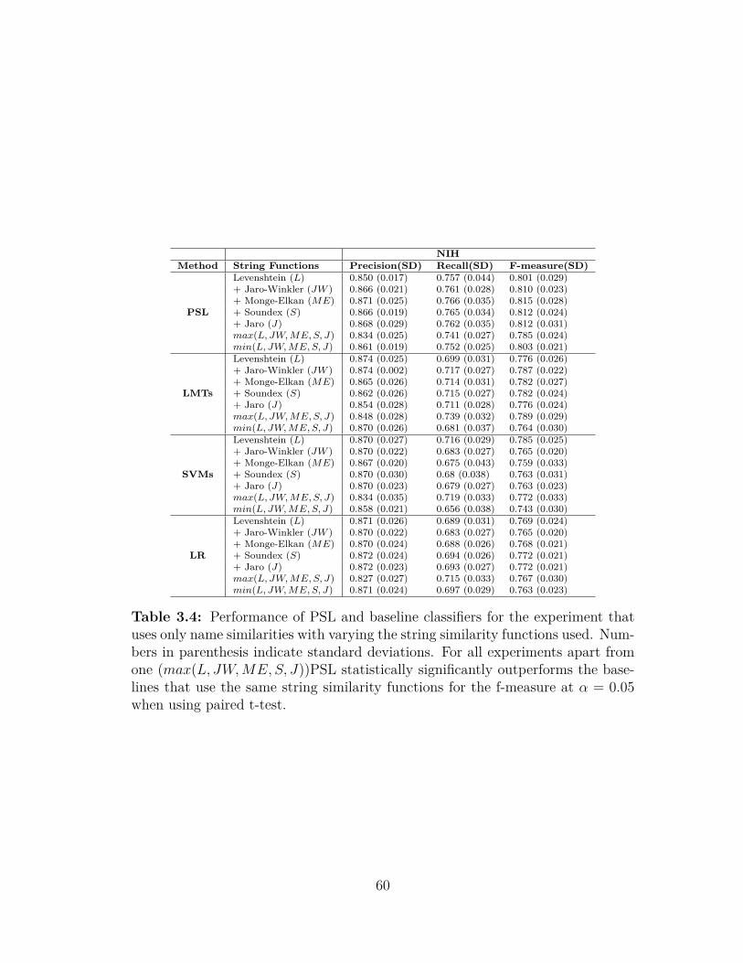
NIHMethod String Functions Precision(SD) Recall(SD) F-measure(SD)

Levenshtein (L) 0.850 (0.017) 0.757 (0.044) 0.801 (0.029)+ Jaro-Winkler (JW ) 0.866 (0.021) 0.761 (0.028) 0.810 (0.023)+ Monge-Elkan (ME) 0.871 (0.025) 0.766 (0.035) 0.815 (0.028)

PSL + Soundex (S) 0.866 (0.019) 0.765 (0.034) 0.812 (0.024)+ Jaro (J) 0.868 (0.029) 0.762 (0.035) 0.812 (0.031)max(L, JW, ME, S, J) 0.834 (0.025) 0.741 (0.027) 0.785 (0.024)min(L, JW, ME, S, J) 0.861 (0.019) 0.752 (0.025) 0.803 (0.021)Levenshtein (L) 0.874 (0.025) 0.699 (0.031) 0.776 (0.026)+ Jaro-Winkler (JW ) 0.874 (0.002) 0.717 (0.027) 0.787 (0.022)+ Monge-Elkan (ME) 0.865 (0.026) 0.714 (0.031) 0.782 (0.027)

LMTs + Soundex (S) 0.862 (0.026) 0.715 (0.027) 0.782 (0.024)+ Jaro (J) 0.854 (0.028) 0.711 (0.028) 0.776 (0.024)max(L, JW, ME, S, J) 0.848 (0.028) 0.739 (0.032) 0.789 (0.029)min(L, JW, ME, S, J) 0.870 (0.026) 0.681 (0.037) 0.764 (0.030)Levenshtein (L) 0.870 (0.027) 0.716 (0.029) 0.785 (0.025)+ Jaro-Winkler (JW ) 0.870 (0.022) 0.683 (0.027) 0.765 (0.020)+ Monge-Elkan (ME) 0.867 (0.020) 0.675 (0.043) 0.759 (0.033)

SVMs + Soundex (S) 0.870 (0.030) 0.68 (0.038) 0.763 (0.031)+ Jaro (J) 0.870 (0.023) 0.679 (0.027) 0.763 (0.023)max(L, JW, ME, S, J) 0.834 (0.035) 0.719 (0.033) 0.772 (0.033)min(L, JW, ME, S, J) 0.858 (0.021) 0.656 (0.038) 0.743 (0.030)Levenshtein (L) 0.871 (0.026) 0.689 (0.031) 0.769 (0.024)+ Jaro-Winkler (JW ) 0.870 (0.022) 0.683 (0.027) 0.765 (0.020)+ Monge-Elkan (ME) 0.870 (0.024) 0.688 (0.026) 0.768 (0.021)

LR + Soundex (S) 0.872 (0.024) 0.694 (0.026) 0.772 (0.021)+ Jaro (J) 0.872 (0.023) 0.693 (0.027) 0.772 (0.021)max(L, JW, ME, S, J) 0.827 (0.027) 0.715 (0.033) 0.767 (0.030)min(L, JW, ME, S, J) 0.871 (0.024) 0.697 (0.029) 0.763 (0.023)

Table 3.4: Performance of PSL and baseline classifiers for the experiment thatuses only name similarities with varying the string similarity functions used. Num-bers in parenthesis indicate standard deviations. For all experiments apart fromone (max(L, JW,ME, S, J))PSL statistically significantly outperforms the base-lines that use the same string similarity functions for the f-measure at α = 0.05when using paired t-test.

60

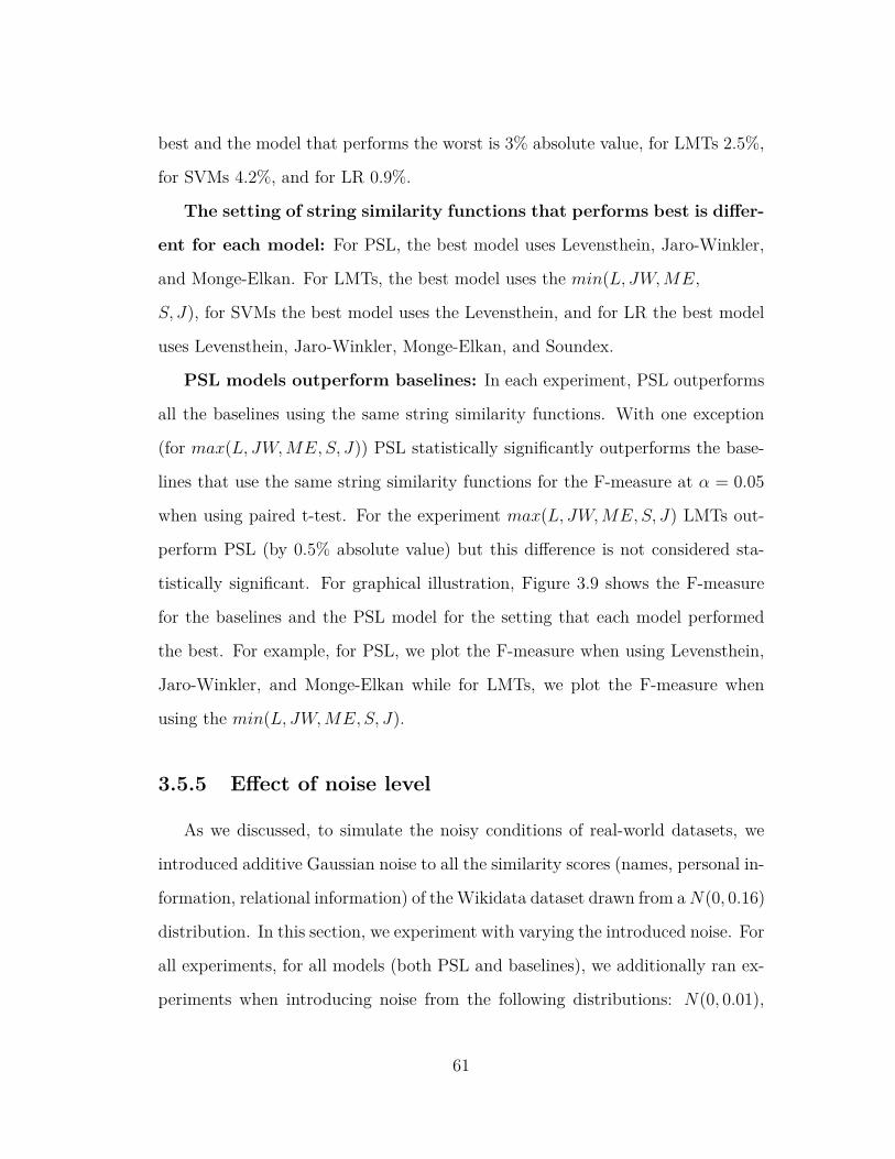
best and the model that performs the worst is 3% absolute value, for LMTs 2.5%,

for SVMs 4.2%, and for LR 0.9%.

The setting of string similarity functions that performs best is differ-

ent for each model: For PSL, the best model uses Levensthein, Jaro-Winkler,

and Monge-Elkan. For LMTs, the best model uses the min(L, JW,ME,

S, J), for SVMs the best model uses the Levensthein, and for LR the best model

uses Levensthein, Jaro-Winkler, Monge-Elkan, and Soundex.

PSL models outperform baselines: In each experiment, PSL outperforms

all the baselines using the same string similarity functions. With one exception

(for max(L, JW,ME, S, J)) PSL statistically significantly outperforms the base-

lines that use the same string similarity functions for the F-measure at α = 0.05

when using paired t-test. For the experiment max(L, JW,ME, S, J) LMTs out-

perform PSL (by 0.5% absolute value) but this difference is not considered sta-

tistically significant. For graphical illustration, Figure 3.9 shows the F-measure

for the baselines and the PSL model for the setting that each model performed

the best. For example, for PSL, we plot the F-measure when using Levensthein,

Jaro-Winkler, and Monge-Elkan while for LMTs, we plot the F-measure when

using the min(L, JW,ME, S, J).

3.5.5 Effect of noise level

As we discussed, to simulate the noisy conditions of real-world datasets, we

introduced additive Gaussian noise to all the similarity scores (names, personal in-

formation, relational information) of theWikidata dataset drawn from aN(0, 0.16)

distribution. In this section, we experiment with varying the introduced noise. For

all experiments, for all models (both PSL and baselines), we additionally ran ex-

periments when introducing noise from the following distributions: N(0, 0.01),

61

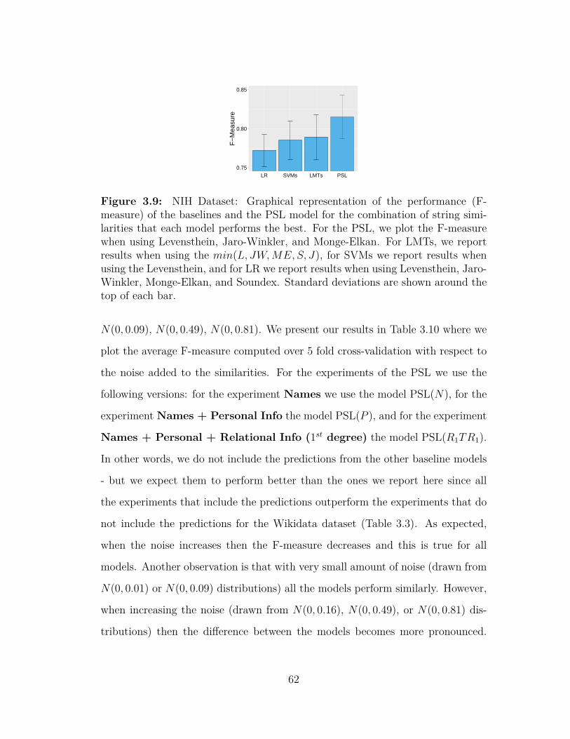
0.75

0.80

0.85

LR SVMs LMTs PSL

F−

Mea

sure

Figure 3.9: NIH Dataset: Graphical representation of the performance (F-measure) of the baselines and the PSL model for the combination of string simi-larities that each model performs the best. For the PSL, we plot the F-measurewhen using Levensthein, Jaro-Winkler, and Monge-Elkan. For LMTs, we reportresults when using the min(L, JW,ME, S, J), for SVMs we report results whenusing the Levensthein, and for LR we report results when using Levensthein, Jaro-Winkler, Monge-Elkan, and Soundex. Standard deviations are shown around thetop of each bar.

N(0, 0.09), N(0, 0.49), N(0, 0.81). We present our results in Table 3.10 where we

plot the average F-measure computed over 5 fold cross-validation with respect to

the noise added to the similarities. For the experiments of the PSL we use the

following versions: for the experiment Names we use the model PSL(N), for the

experiment Names + Personal Info the model PSL(P ), and for the experiment

Names + Personal + Relational Info (1st degree) the model PSL(R1TR1).

In other words, we do not include the predictions from the other baseline models

- but we expect them to perform better than the ones we report here since all

the experiments that include the predictions outperform the experiments that do

not include the predictions for the Wikidata dataset (Table 3.3). As expected,

when the noise increases then the F-measure decreases and this is true for all

models. Another observation is that with very small amount of noise (drawn from

N(0, 0.01) or N(0, 0.09) distributions) all the models perform similarly. However,

when increasing the noise (drawn from N(0, 0.16), N(0, 0.49), or N(0, 0.81) dis-

tributions) then the difference between the models becomes more pronounced.

62

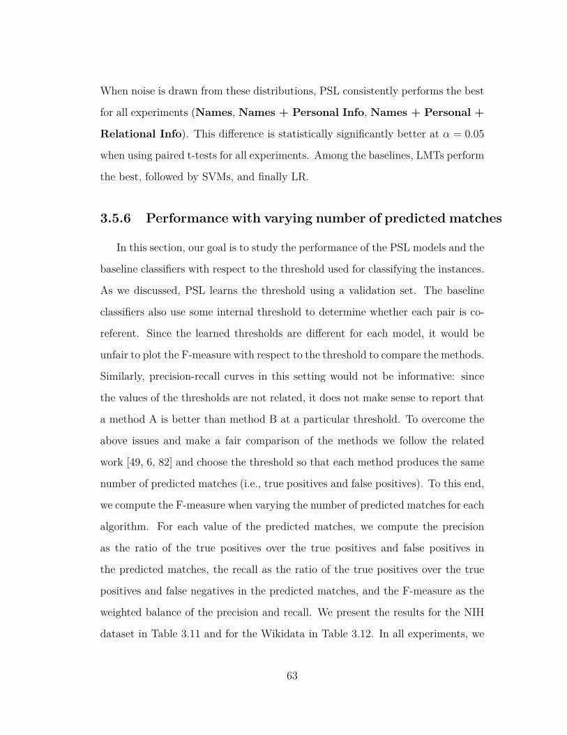
When noise is drawn from these distributions, PSL consistently performs the best

for all experiments (Names, Names + Personal Info, Names + Personal +

Relational Info). This difference is statistically significantly better at α = 0.05

when using paired t-tests for all experiments. Among the baselines, LMTs perform

the best, followed by SVMs, and finally LR.

3.5.6 Performance with varying number of predicted matches

In this section, our goal is to study the performance of the PSL models and the

baseline classifiers with respect to the threshold used for classifying the instances.

As we discussed, PSL learns the threshold using a validation set. The baseline

classifiers also use some internal threshold to determine whether each pair is co-

referent. Since the learned thresholds are different for each model, it would be

unfair to plot the F-measure with respect to the threshold to compare the methods.

Similarly, precision-recall curves in this setting would not be informative: since

the values of the thresholds are not related, it does not make sense to report that

a method A is better than method B at a particular threshold. To overcome the

above issues and make a fair comparison of the methods we follow the related

work [49, 6, 82] and choose the threshold so that each method produces the same

number of predicted matches (i.e., true positives and false positives). To this end,

we compute the F-measure when varying the number of predicted matches for each

algorithm. For each value of the predicted matches, we compute the precision

as the ratio of the true positives over the true positives and false positives in

the predicted matches, the recall as the ratio of the true positives over the true

positives and false negatives in the predicted matches, and the F-measure as the

weighted balance of the precision and recall. We present the results for the NIH

dataset in Table 3.11 and for the Wikidata in Table 3.12. In all experiments, we

63

0.6

0.7

0.8

0.9

0 0.1 0.2 0.3 0.4 0.5 0.6 0.7 0.8

F-m

ea

su

re

σ2 of noise N(0, σ

2)

Experiment: Names

LRSVMsLMTs

PSL

(a)

0.6

0.7

0.8

0.9

0 0.1 0.2 0.3 0.4 0.5 0.6 0.7 0.8

F-m

ea

su

reσ

2 of noise N(0, σ

2)

Experiment: Names + Personal Info

LRSVMsLMTs

PSL

(b)

0.6

0.7

0.8

0.9

0 0.1 0.2 0.3 0.4 0.5 0.6 0.7 0.8

F-m

ea

su

re

σ2 of noise N(0, σ

2)

Experiment: Names + Personal + Relational Info

LRSVMsLMTs

PSL

(c)

Figure 3.10: An analysis of the performance of the models (PSL and baselines)when varying the noise in the similarities for the Wikidata dataset (for the ex-periments (a) Names, (b) Names + Personal Info, (c) Names + Personal+ Relational Info (1st degree)). We report average F-measure scores from a5-fold cross validation. As the noise increases, the F-measure decreases. For theminimum amount of noise all the models perform similarly. However, as the noiseincreases the difference in the performance becomes more evident.

64

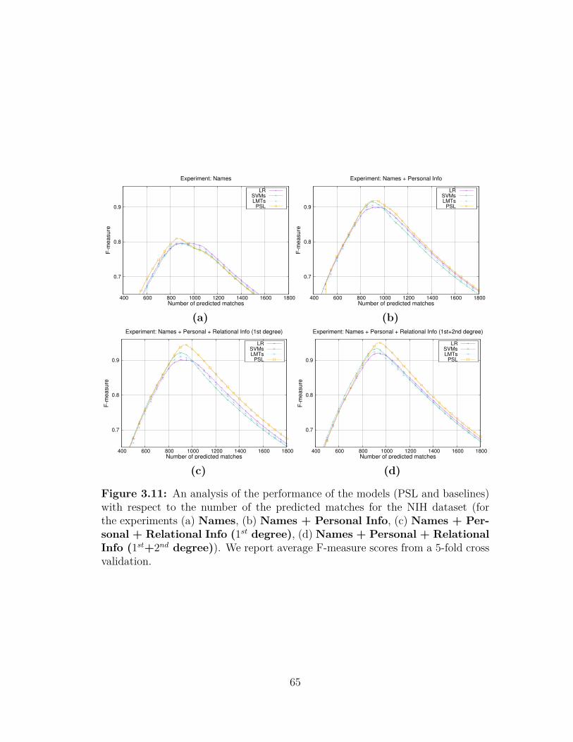
0.7

0.8

0.9

400 600 800 1000 1200 1400 1600 1800

F-m

ea

su

re

Number of predicted matches

Experiment: Names

LRSVMsLMTs

PSL

(a)

0.7

0.8

0.9

400 600 800 1000 1200 1400 1600 1800F

-me

asu

reNumber of predicted matches

Experiment: Names + Personal Info

LRSVMsLMTs

PSL

(b)

0.7

0.8

0.9

400 600 800 1000 1200 1400 1600 1800

F-m

ea

su

re

Number of predicted matches

Experiment: Names + Personal + Relational Info (1st degree)

LRSVMsLMTs

PSL

(c)

0.7

0.8

0.9

400 600 800 1000 1200 1400 1600 1800

F-m

ea

su

re

Number of predicted matches

Experiment: Names + Personal + Relational Info (1st+2nd degree)

LRSVMsLMTs

PSL

(d)

Figure 3.11: An analysis of the performance of the models (PSL and baselines)with respect to the number of the predicted matches for the NIH dataset (forthe experiments (a) Names, (b) Names + Personal Info, (c) Names + Per-sonal + Relational Info (1st degree), (d) Names + Personal + RelationalInfo (1st+2nd degree)). We report average F-measure scores from a 5-fold crossvalidation.

65

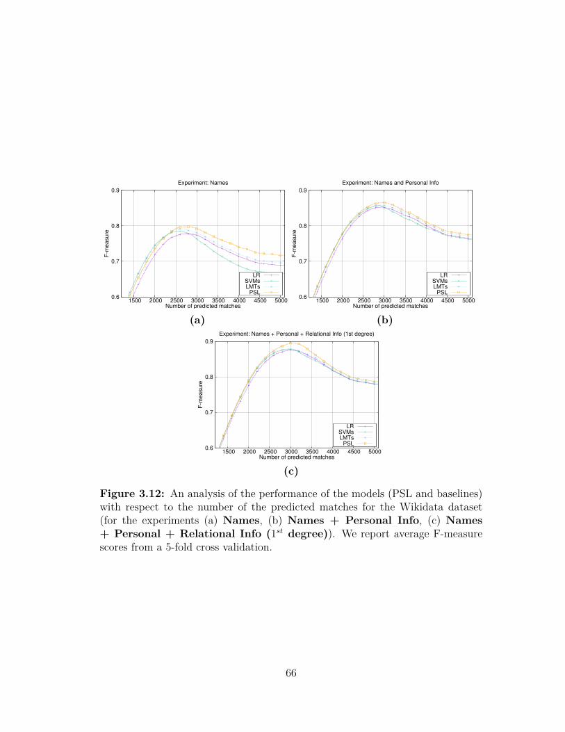
0.6

0.7

0.8

0.9

1500 2000 2500 3000 3500 4000 4500 5000

F-m

ea

su

re

Number of predicted matches

Experiment: Names

LRSVMsLMTs

PSL

(a)

0.6

0.7

0.8

0.9

1500 2000 2500 3000 3500 4000 4500 5000F

-me

asu

re

Number of predicted matches

Experiment: Names and Personal Info

LRSVMsLMTs

PSL

(b)

0.6

0.7

0.8

0.9

1500 2000 2500 3000 3500 4000 4500 5000

F-m

ea

su

re

Number of predicted matches

Experiment: Names + Personal + Relational Info (1st degree)

LRSVMsLMTs

PSL

(c)

Figure 3.12: An analysis of the performance of the models (PSL and baselines)with respect to the number of the predicted matches for the Wikidata dataset(for the experiments (a) Names, (b) Names + Personal Info, (c) Names+ Personal + Relational Info (1st degree)). We report average F-measurescores from a 5-fold cross validation.

66

report the results of the PSL models that include the predictions of the other

classifiers. More specifically, we report the results of the models: PSL(N + pred),

PSL(P +pred), PSL(R1TR1 +pred), and PSL(R12TR12 +pred) (only for the NIH

dataset).

For the NIH dataset, for the experiment Names, we observe that PSL consis-

tently outperforms all the baselines when the number of matches is smaller than

950. However, when the number of matches is larger than 1000 the performance

of the PSL is lower than the baselines. For all the other experiments (Names

+ Personal Info, Names + Personal + Relational Info (1st degree), and

Names + Personal + Relational Info (1st + 2nd degree)) all models perform

similarly when the number of predicted matches is smaller than 800. When the

number of predicted matches is larger than 800 we can see that the PSL models

consistently outperform all the baselines. For the Wikidata dataset, for all the

experiments we observe that all the models perform similarly for small number

of matches (up to 2500). However, when the number of matches increases (i.e.,

larger than 2500) then we observe a clear win of the PSL models.

3.6 Other Applications: Recommender Systems

In this section, we show how we can apply our approach to the domain of

recommender systems and, in particular, to the items of the user-item recommen-

dation matrix. Identifying the coreferent items allows for increasing the density

of the user-item matrix. In addition to improving accuracy, finding the coref-

erent items enables us to address an additional problem inherent to the area of

recommender systems: the cold-start problem. More specifically, inferring that a

newly-added item is coreferent with an existing already-rated item enables us to

recommend the new item without the need for ratings from users.

67

Entity resolution in the recommender systems setting (e.g., products) is a

very challenging task, since it is not straightforward whether two items should be

merged. For example, two cameras varying in their color may appear twice on a

web site, but may correspond to the exact same model. In this case, it is unclear

whether those two products should be resolved, because some users may not be

interested in the color of the camera but only in the technical specifications, while

others may consider the color more important than the technical specifications.

For the first group of users, the two cameras are the same product, so merging

them would be beneficial since it will increase the density of the the user-item

matrix. On the other hand, for the second group of users merging the two products

may be a sub-optimal decision.

In this section, we describe how we can perform entity resolution for products

with a focus on the cold-start problem. The basic idea is that we should re-

solve products with very similar characteristics (e.g., similar names, description,

reviews) only if they have a very small number of ratings. Once those products

acquire a sufficient number of ratings by users then we should treat them as sepa-

rate products. The reasoning behind this approach can be explained best through

an example: consider that there is a very succesfull camera (e.g., “Nikon D3400”)

with a large number of ratings and a new version becomes available (e.g., “Nikon

D3500”). Both cameras are of the same brand and have very similar character-

istics. When the new version of the camera becomes available for sale, it has no

ratings, so merging it with the previous version of the camera can help provide

some ratings. However, once the new version gets a sufficient number of ratings,

then we can recommend the new camera based only on the ratings for this new

version.

68

3.6.1 Problem Formulation for Entity Resolution in Rec-

ommender Systems

In a typical recommender system setting, there is a set of users U = {u1, u2, ...,

uk}, a set of items I = {i1, i2, ..., in}, and a set of observed ratingsR, i.e., recorded

ratings from a subset of users U to a subset of items I. Given the above, the task is

to perform rating prediction, i.e., predict the values of a set of unobserved ratings

R′.

In our setting, we consider an entity resultion step that we need to perform

before the recommender system problem. More specifically, the given set of items

I oftentimes contains duplicates. We refer to this set as a set of references I where

each reference has attributes i.A1, i.A2, i.Ak. The references correspond to a set of

unknown entities E = {em} which is the set of unique items. The duplicate items

that have been resolved map to the same entity in E . We introduce the attribute

i.E to refer to the entity to which reference i corresponds to. The first part of

the problem is to recover the hidden set of entities E = {em} and the entity labels

i.E for individual references given the observed attributes of the references. We

note that the set of entities E = {em} should be regularly updated based on the

available number of ratings for each item i. The second part of the problem is how

to exploit the discovered entity set E in order to improve the rating prediction

task.

3.6.2 Entity Resolution Task

To discover the hidden set of entities we extend the model of Section 3.4.

We first introduce a latent variable SameLatent(p1, p2) whose value represents

the probability that two products are coreferent independent from the number of

ratings. To compute the value of this latent variable, we start by introducing rules

69

that can capture similar product names, similar product description, and similar

price. These rules can be defined as follows.

SimNameSIM(p1, p2)⇒ SameLatent(p1, p2)

SimPriceSIM(p1, p2)⇒ SameLatent(p1, p2)

SimDescriptionSIM(p1, p2)⇒ SameLatent(p1, p2) .

The notation is similar to the notation used in Section 3.4. To compute name,

price, and description similarity we can use different similarity metrics SIM like

in the case of entity resolution in familial networks.

Additionally, we can use simple relational information in order to disallow

matches of different products. For example we can model the intuition that two

products that belong to different categories (e.g., the movie “Twinlight” with the

book “Twinlight”) should not be merged as follows:

¬BelongToDifferentCategory(p1, p2)⇒ ¬SameLatent(p1, p2) .

Furthermore, we can use more complicated relational information when avail-

able. For example, big eCommerce websites such as Amazon.com provide parent-

child relationships that can be further exploited. In Amazon.com, each parent-child

relationship has three basic elements: the parent product, the child product, and

the variation theme. A parent product is a non-buyable product used to relate

child products. The Amazon catalog uses the parent product to establish relation-

ships between the child products. For example, if two shirts have the same parent

then they are related and are considered child products. The child product is an

instance of the parent product. We can have many child products that are all re-

lated to one parent product. Each child varies in some way, for example, by size or

70

by color. The variation theme defines how related products differ from each other.

For example, in the “Clothing, Accessories and Luggage” category, child products

can differ from each other by size or color. We can leverage the above relational

information with a special care when using the variation theme. For example,

for the category “Clothing, Accessories and Luggage” two products with different

size should probably be considered as the same, however, this is not true for two

products with different colors (for example, there may be a user that hates the

black color but loves the purple color). To this end, we need first to define which

variation themes allow for merging and which do not allow for merging. We can

do this by introducing the predicate ImportantVariationalTheme(t) which

is true if the theme t is considered an important differentiator for two products

(such as color) and false if the theme t is not considered an important differen-

tiator for two products (such as size). We can introduce rules that capture the

intuition that if two products belong to the same parent category and have dif-

ferent variational theme and the variation theme is considered as an important

differentiator then the products should not be merged as follows:

BelongToTheSameParent(p1, p2) ∧ ImportantVariationalTheme(t)

∧BelongsToVariationalTheme(p1, t1)∧

∧BelongsToVariationalTheme(p2, t2) ∧ t1 6= t2 ⇒

¬SameLatent(p1, p2) .

Similarly, we can add the inverse rule that captures the intuition that if two

products belong to the same parent category and have different variational theme

and the variation theme is not considered as an important differentiator then the

products should be merged as follows:

71

BelongToTheSameParent(p1, p2) ∧ ¬ImportantVariationalTheme(t)

∧BelongsToVariationalTheme(p1, t1)∧

∧BelongsToVariationalTheme(p2, t2) ∧ t1 6= t2 ⇒

SameLatent(p1, p2) .

Additionally, we can introduce transitive relational rules that allow for collec-

tive classification. For example, for the case of complementary products, we can

capture the intuition that if we have strong evidence that two products are the

same, then their complementary products should also be the same when addi-

tional evidence is also available, e.g., if their names are similar. An example of

complementary products can be a cell phone with its charger. If we have strong

evidence that two cell phones belong to the same entity and their complemen-

tary products have very similar names then we can infer that the complementary

products belong to the same entity. The following intuition can be captured by

the following rule:

ComplementaryProducts(p1, pa) ∧ComplementaryProducts(p2, pb)∧

SameLatent(p1, p2) ∧ SimNameSIM(pa, pb)⇒ SameLatent(pa, pb) .

Finally, to capture the fact that we want to merge products for the cases where

the value of the latent variable SameLatent(p1, p2) is high and at the same time

one product has a sufficient number of ratings, while the other has limited ratings,

we introduce the predicate ColdStartItem(p1). This predicate is true if the

product has a number of ratings below a threshold and false if the product has a

number of ratings above a threshold. We introduce the following rule to merge an

item that has limited number of ratings with an item that has a sufficient number

of ratings:

72

¬ColdStartItem(p1) ∧ColdStartItem(p2) ∧ SameLatent(p1, p2)

⇒ Same(p1, p2) .

3.6.3 Rating Prediction Task

For the rating prediction task, instead of using the set of items I which may

contain duplicate items, we propose to use the set of the resolved items E produced

during the entity resolution task. So, for each item i ∈ I we will use the entity

that corresponds to, i.e. i.E. As a result, the new set of items that will be given

as input to the recommender system is I ′ = {i1.E, i2.E, ..., in.E}. The set of users

and observed ratings will stay the same.

3.7 Conclusions and Future Work

Entity resolution in familial networks poses several challenges, including het-

erogeneous relationships that introduce collective dependencies between decisions

and inaccurate attribute values that undermine classical approaches. In this work,

we propose a scalable collective approach based on probabilistic soft logic that

leverages attribute similarities, relational information, logical constraints, and

predictions from other algorithms. A key differentiator of our approach is the

ability to support bijection and different types of transitive relational rules that

can model the complex familial relationships. Moreover, our method is capa-

ble of using training data to learn the weight of different similarity scores and

relational features, an important ingredient of relational entity resolution. In

our experimental evaluation, we demonstrated that our framework can effectively

combine different signals, resulting in improved performance over state-of-the-art

approaches on two datasets. In our experimental evaluation, we also showed that,

73

in most cases, our model outperforms the baselines for a varying set of similarity

functions and for varying levels of noise. Additionally, the experimental evaluation

showed that the PSL models outperform the baselines when we fix the number of

predicted matches.

In this paper, we motivate the importance of our approach with an application

for resolving mentions in healthcare records. We additionally showed how we can

extend the proposed framework to the domain of recommender systems to resolve

products. However, the problem of entity resolution in richly structured domains

has many additional applications. In domains similar to healthcare, companies

such as ancestry.com, genealogy.com, familysearch.org, and 23andMe.com

provide genealogical discovery services, which require a similar entity resolution

process. In addition, our approach can be very beneficial to applications in so-

cial networks where linking user accounts across several social platforms in the

presence of a diverse set of relationships (e.g., friends, followers, followees, family

cycles, shared groups), ambiguous names, and collective constraints such as bi-

jection and transitivity, can provide great performance gains and improved user

experience as we discuss in the next section.

In future work, we plan to apply our approach to a broader set of problems and

discuss general strategies for multirelational entity resolution. Additionally, we

plan to explore structured output learning techniques [85] inside PSL. Such tech-

niques can directly consider the matching constraints during the learning phase

instead of post processing the classification results. We also plan to explore tem-

poral relations, e.g. ex-wife, and more complex relationships, e.g. adopted child.

Finally, in certain cases, we might inadvertently introduce inaccurate relations

when following the approach of Section 3.3. To address this, we plan to expand

our work to account for uncertainty in the relational normalization step by as-

74

suming a probability assigned to each populated relationship instead of the hard

values that we currently assign.

75

Chapter 4

Recommendations in Richly

Structured Social Networks

Recent work on hybrid recommender systems has shown that recommendation

accuracy can be improved by combining multiple data modalities and modeling

techniques within a single model [2, 26, 27, 75, 77]. Existing hybrid recommender

systems are typically designed for a specific problem domain, such as movie rec-

ommendations, and are limited in their ability to generalize to other settings or

make use of any further information. As our daily lives become increasingly digi-

tally connected, the list of data sources available for recommendations continues

to grow. There is a need for general-purpose, extensible frameworks that can

make use of arbitrary data modalities to improve recommendation.

The challenge of custom model-building has been extensively studied in the

fields of probabilistic programming [45] and statistical relational learning (SRL)

[43], which provide programming language interfaces for encoding knowledge and

specifying models. Probabilistic programs can be used to encode graphical models

for reasoning with graph-structured probabilistic dependencies. Graphical models

are a natural approach to recommendations given that the user-item rating ma-

76

trix can be interpreted as a graph, with weighted edges between users and items

corresponding to the respective ratings [27].

In modern recommendation contexts, a bipartite user-item graph is insufficient

to represent all available information, such as user-user and item-item similarity,

content, social information, and metadata. For example, neighborhood-based

collaborative filtering techniques can be interpreted as predicting ratings based

on an extension of the user-item graph with additional edges between pairs of

similar users or similar items (Figure 4.1). We need a more general representation

to reason over this richly structured information.

In this work, we propose a general hybrid recommender framework, called Hy-

PER (HYbrid Probabilistic Extensible Recommender), which leverages the flex-

ibility of probabilistic programming in order to build adaptable and extensible

hybrid recommender systems which reason over complex data. In particular, we

use probabilistic soft logic (PSL) which was described in detail in Chapter 2. We

reiterate that PSL is especially well-suited to collaborative-filtering based rec-

ommendation graphs as it is able to fuse information from multiple sources and

it was originally designed as a flexible framework for reasoning and combining

similarities [12]. It provides a general declarative framework for combining entity

similarities, attribute similarities, and information from additional sources includ-

ing the predictions of other algorithms. As discussed, PSL allows for efficient and

scalable inference, which is crucial in a recommendation context.

Our contributions include (1) a general and extensible hybrid recommender

system with a probabilistic programming interface, (2) a method for learning how

to balance the different input signals in the hybrid system, and (3) extensive

experimental studies using several information sources which validate the perfor-

mance of the proposed framework and highlight contribution of each source to the

77

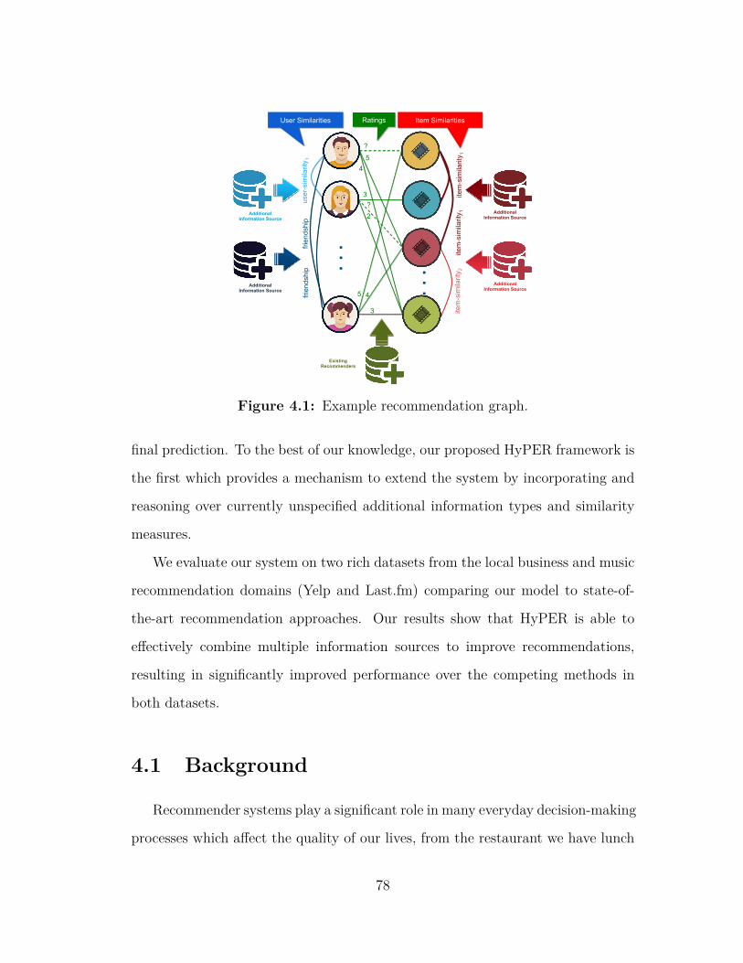
User Similarities Item Similarities

5

?

?

4

4 5

3

3

. . .

Ratings

. . .

2

frien

dshi

p fri

ends

hip

user

-sim

ilarit

y 1

item

-sim

ilarit

y 1

item

-sim

ilarit

y 1

item

-sim

ilarit

y 2

Additional Information Source

Additional Information Source

Additional Information Source

Additional Information Source

Existing Recommenders

Figure 4.1: Example recommendation graph.

final prediction. To the best of our knowledge, our proposed HyPER framework is

the first which provides a mechanism to extend the system by incorporating and

reasoning over currently unspecified additional information types and similarity

measures.

We evaluate our system on two rich datasets from the local business and music

recommendation domains (Yelp and Last.fm) comparing our model to state-of-

the-art recommendation approaches. Our results show that HyPER is able to

effectively combine multiple information sources to improve recommendations,

resulting in significantly improved performance over the competing methods in

both datasets.

4.1 Background

Recommender systems play a significant role in many everyday decision-making

processes which affect the quality of our lives, from the restaurant we have lunch

78

at, to the hotel for our vacation, to the music we listen to. Traditional rec-

ommender systems primarily leverage underlying similarities between users and

items in order to make predictions based on observed ratings. Content-based

filtering (CB) approaches compute these similarities by using features extracted

from content to build user profiles, which are compared with content features of

items. While content-based approaches can recommend newly added items, they

are limited by a lack of serendipity. The recommendations are limited to the

user’s known likes and do not generally include items out of the user’s (recorded)

comfort zone [76].

Collaborative filtering (CF) techniques address this by identifying similar users

or items based on their rating patterns instead of content, using methods such as

neighborhood-based approaches and matrix factorization models. However, col-

laborative filtering methods typically do not perform well in “cold-start” settings,

where there are few ratings for a user or an item [64]. Moreover, pure rating-

based collaborative filtering approaches cannot take advantage of data which may

be available in addition to ratings.

To address these shortcomings, hybrid recommender systems (HRSs) were

introduced, combining content-based and collaborative-filtering techniques (e.g.

[2, 26, 27]). HRS techniques can improve performance over content-based and

collaborative filtering methods alone, especially in the case where the ratings

matrix is sparse [2]. However, existing HRSs have their own limitations. First,

they are problem- and data-specific. Each HRS is typically motivated by a specific

problem domain (e.g. movie recommendations) and the solution is fine-tuned to

solve a specific problem with datasets of specific characteristics. Hence, HRSs

typically cannot be generalized to different problem domains or input data, or be

easily expanded to incorporate knowledge from richer datasets.

79

As the web has evolved into a participatory, user-driven platform, additional

information is increasingly becoming available. Users form social networks, give

verbal feedback on items via reviews, endorse or down-vote items or other users,

form trust relationships, “check-in” at venues, and perform many other social

actions that may potentially be leveraged to better understand users in order to

improve recommendations. A flexible and extensible hybrid recommender system

which can make use of this wealth of information is increasingly important.

The remainder of this Chapter is structured as follows. In Section 4.2, we place

our system in the context of related work. In Section 4.3 we introduce HyPER, a

general hybrid recommendation framework which is extensible and customizable

using PSL. We systematically evaluate our framework in Section 4.4. Finally, we

conclude with a discussion and future plans in Section 4.5.

4.2 Related Work

There is a large body of work on recommender systems; see Ricci et al. [100]

for an overview. We focus our related work discussion on hybrid recommender

systems, and particularly systems that can incorporate richly structured and social

data as well as graphical modeling approaches. In Burke [13]’s taxonomy of hybrid

recommender systems our work falls into the “feature augmentation” category.

Hybrid systems typically combine two or more approaches in order to pro-

vide better recommendations, usually content-based and collaborative filtering

approaches [47, 37] or variations of collaborative filtering approaches [61]. Gu-

nawardana and Meek [47] present a domain-agnostic hybrid approach for using

content to improve item-item modeling. After the Netflix Prize competition, en-

semble methods [57] have gained popularity. Factorization Machines [98] are a

general matrix factorization method that can be applied to design hybrid fac-

80

torization models. Recently, as user-generated content has become available, re-

searchers have studied how to leverage information such as social relationships

[75, 77], reviews [78, 74], tags [48], and feedback [103] to improve recommenda-

tions. Incorporating additional information for users and/or items is especially

beneficial in cold-start settings [41]. Dooms [31] argues that a flexible recom-

mendation system that automatically generates good hybrid models would be

very valuable as information sources increase. Our model provides such flexibil-

ity, allowing for the combination of as many information sources as are available.

Fakhraei et al. [35] use PSL to reason over multiple similarity measures for pre-

dicting drug-target interactions.

Chen at al. [21] learn the strength of ties between users based on multi-

relational network information. The learned network is combined with item-based

collaborative filtering to improve recommendation results. Burke et al. [14, 42]

integrate different dimensions of data about users in a heterogeneous network by

using metapaths to create multiple two-dimensional projections representing re-

lationships between entities (e.g. users-tags) and then linearly combining these

projections. Also using metapaths, Yu et al. [118] propose a global and a personal-

ized recommendation model. In their approach, implicit feedback is incorporated

into metapaths and latent features for users and items are generated using matrix

factorization.

De Campos et al. [26] propose a probabilistic graphical modeling recommen-

dation approach using Bayesian networks. Their approach combines individual

predictions from content-based and user-based collaborative filtering components.

Hoxha and Rettinger [54] also discuss a probabilistic graphical modeling repre-

sentation, using Markov Logic Networks (MLNs) [101] to combine content with

collaborative filtering. Both MLNs and HL-MRFs operate on undirected graphical

81

models using a first-order logic as their template language, while Bayesian net-

works are directed. We chose HL-MRFs because they can represent ordered data

such as ratings, and due to their scalability with parallel convex optimization for

inference. Speed and scalability is of paramount importance in recommender sys-

tems and in particular when we run the prediction task collectively over multiple

types of input data with a variety of similarity measures.

4.3 Proposed Solution

We propose HyPER, a general hybrid framework that combines multiple dif-

ferent sources of information and modeling techniques into a single unified model.

HyPER offers the capability to extend the model by incorporating additional

sources of information as they become available. Our approach begins by viewing

the recommendation task as a bipartite graph, where users U and items I are the

vertices, and ratings are edges between users and items [27]. Using PSL [4], a

flexible statistical relational learning system with a probabilistic programming in-

terface, this graph is then augmented to construct a probabilistic graphical model

with additional edges to encode similarity information, predicted ratings, content

and social information, and metadata. We then train the graphical model to

learn the relative importance of the different information sources in the hybrid

system, and make predictions for target ratings, using graphical model learning

and collective inference techniques.

Figure 4.1 shows an overview of our modeling approach. In the figure, items

and users are nodes, and green edges represent the ratings that users gave to items,

with edge weights corresponding to the rating values. The goal is to predict the

edge weights for unobserved edges, denoted as dashed lines. Neighborhood-based

approaches find the k most similar users or similar items, and use their ratings

82

to make these predictions. In our graph-based representation, we interpret these

k-nearest neighbor relationships as k edges which are added to the graph. In

Figure 4.1, blue edges encode user similarities and red edges correspond to item

similarities.

We can further encode additional sources of information and outputs of other

recommendation algorithms within this graph-based representation in a similar

way, i.e. in the form of additional links or nodes. For instance, latent factor

methods identify latent representations which can be used to augment the graph

with weighted edges encoding predictions of user-item ratings based on the latent

space. The latent representations can also be used to construct additional user-

user and item-item edges by identifying similar users and similar items in the

latent space. Content information and metadata, such as demographics and time

information, can be incorporated in the graph representation by identifying further

similarity links, or by adding nodes with attribute values, and edges to associate

these values with users and items. Furthermore, social information from digital

social media is inherently relational, and can readily be incorporated into a graph-

based representation.

Having encoded all available information in the graph, the next step is to

reason over this graph to predict unobserved user-item rating edges. We view the

prediction task as inference in a graphical model, the structure of which is defined

by our graph representation. We use the PSL framework, introduced in Chapter

2, to define a probability distribution over unobserved ratings. In the next section

we describe in detail our unified recommender system modeling framework.

83

4.3.1 PSL Model for Hybrid Recommender Systems

The strengths of the HyPER framework include the ability to extensibly incor-

porate multiple sources of information in a unified hybrid recommendation model,

as well as learning how to balance these signals from training data. HyPER models

are specified using a collection of PSL rules which encode graph-structured depen-

dency relationships between users, items, ratings, content and social information.

Additionally, the model provides the flexibility to incorporate prior predictions,

such as mean-centering predictors and the results of other recommendation algo-

rithms. In what follows, we present the rules that define the HL-MRF model for

the core of the HyPER framework. We emphasize that while this set of rules cov-

ers a breadth of input sources, the model can be readily extended to incorporate

other sources of information such as time, implicit feedback, and social interac-

tions, with the introduction of new PSL rules. Moreover, additional similarity

measures and recommendation algorithms can straightforwardly be included with

analogous rules.

User-based Collaborative Filtering

Motivated by the basic principles of the neighborhood-based approach, we can

define PSL rules of this form:

SimilarUserssim(u1, u2) ∧Rating(u1, i)⇒ Rating(u2, i) .

This rule captures the intuition that similar users give similar ratings to the

same items. The predicate Rating(u, i) takes a value in the interval [0, 1] and

represents the normalized value of the rating that a user u gave to an item i,

while SimilarUserssim(u1, u2) is binary, with value 1 iff u1 is one of the k-nearest

neighbors of u2. The similarities can be calculated with any similarity measure

84

sim, as we will describe in Section 4.3.1. The above rule represents a template for

hinge functions which reduce the probability of predicted ratings as the difference

between Rating(u2, i) and Rating(u1, i) increases, for users that are neighbors.

Item-based Collaborative Filtering

Similarly, we can define PSL rules to capture the intuition of item-based col-

laborative filtering methods, namely that similar items should have similar ratings

from the same users:

SimilarItemssim(i1, i2) ∧Rating(u, i1)⇒ Rating(u, i2) .

The predicate SimilarItemssim(i1, i2) is binary, with value 1 iff i1 is one of

the k-nearest neighbors of i2 (using similarity measure sim), while Rating(u, i)

represents the normalized value of the rating of user u to item i, as discussed

above.

Combining Collaborative Filtering Measures

By including both types of rules described in Sections 4.3.1 and 4.3.1 we can

define an HL-MRF model that combines user-based and item-based techniques

to predict ratings. There exist many measures available to compute similarities

between entities for user-based and item-based methods, and these different mea-

sures capture different notions of similarity. For instance, in neighborhood-based

approaches, vector-based similarity measures are broadly used, whereas in latent

factor approaches other similarities, applicable to the low dimensional space, are

preferred. While most existing recommender systems are designed to use a single

similarity measure, HyPER allows for the simultaneous incorporation of multiple

similarity measures, and can automatically adjust the importance of each based

on training data.

85

In this instantiation of our HyPER framework we use the most popular simi-

larity measures in the neighborhood-based recommendations literature [27]. More

specifically, we apply Pearson’s correlation and cosine similarity measures to cal-

culate similarities between users and items; for the items we additionally apply

the adjusted cosine similarity measure. To incorporate matrix-factorization col-

laborative filtering, and inspired by Hoff et al. [53], we compute similar users and

items in the low-dimensional latent space using two popular distance measures

in that space, namely, cosine and Euclidean. The user similarities are identified

using the following rules:

SimilarUserscosine(u1, u2) ∧Rating(u1, i)⇒ Rating(u2, i)

SimilarUserspearson(u1, u2) ∧Rating(u1, i)⇒ Rating(u2, i)

SimilarUserslatentcosine

(u1, u2) ∧Rating(u1, i)⇒ Rating(u2, i)

SimilarUsers latenteuclidean

(u1, u2) ∧Rating(u1, i)⇒ Rating(u2, i) .

Analogous rules are introduced to identify similar items, but are omitted due

to space limitations. As noted earlier, this initial set of similarity measures can

be readily expanded by adding the corresponding rules, in the same form as above.

Mean-Centering Priors

Each individual user considered in a recommender system has her own biases

in rating items (e.g. some users tend to be stricter than others). Moreover, each

item’s rating is influenced by its overall quality and popularity (e.g. a popular

blockbuster may get higher ratings on average than a low-budget movie). To

address such biases, a recommender system needs to incorporate a normalization

mechanism, both per user, and per item. Using mean-centering normalization

for neighborhood-based approaches, or including intercept terms in probabilistic

86

latent factor models, addresses this issue and generally improves performance [27].

In our HyPER framework we encode this intuition with rules that encourage the

ratings to be close to the average, per-user and per-item:

AverageUserRating(u)⇒ Rating(u, i)

¬AverageUserRating(u)⇒ ¬Rating(u, i)

AverageItemRating(i)⇒ Rating(u, i)

¬AverageItemRating(i)⇒ ¬Rating(u, i) .

The predicate AverageUserRating(u) represents the average of the ratings

over the set of items that user u provided in the training set.

Similarly, AverageUserRating(i) represents the average of the user ratings an

item i has received. The pair of PSL rules per-user and per-item corresponds to a

“V-shaped” function centered at the average rating, which penalizes the predicted

rating for being different in either direction from this average.

In order to capture cases where we have no information about a user or an

item, we use a general prior rating centered at the average value of all of the

ratings in the system (i.e. the average over all items rated by all users). We

encode this prior with the following rules:

PriorRating⇒ Rating(u, i)

¬PriorRating⇒¬Rating(u, i) .

The real-valued predicate PriorRating represents the average of all of the rat-

ings.

Using Additional Sources of Information

Incorporating other sources of information pertaining to items, users, and their

respective ratings to our framework is straightforward. In the present instantiation

87

of our framework, we use the content of the items to find similar items:

SimilarItemsContent(i1, i2) ∧Rating(u, i1)⇒ Rating(u, i2) .

In this rule, the predicate SimilarItemsContent(i1, i2) represents items that have

similar content-based features (e.g. in the movie recommendation domain such

features are the genre, actor, director, etc.), instead of similar ratings.

The HyPER framework can also incorporate social information, when this is

available. For instance, in the present instantiation of the system, we leverage

social network friendship links as follows:

Friends(u1, u2) ∧Rating(u1, i)⇒ Rating(u2, i) .

Note that our framework is flexible and can incorporate many other sources

of information that are available. For instance, we can leverage demographic

information by computing similarity neighborhood relationships in demographic

feature space and employing the rule:

SimilarUsersDemo(u1, u2) ∧Rating(u1, i)⇒ Rating(u2, i) .

Leveraging Existing Recommendation Algorithms

Every recommendation algorithm has strengths and weaknesses which may

depend on data-specific factors such as the degree of sparsity or the shape of the

data matrix. This imposes a big limitation in the recommendation process, as

choosing one algorithm as the core of a recommender system limits its strength to

a particular set of domains. In this work, our motivation is to provide a flexible

framework that can be used as-is to generate accurate recommendations for any

domain and data regime. Therefore, instead of selecting a single recommendation

88

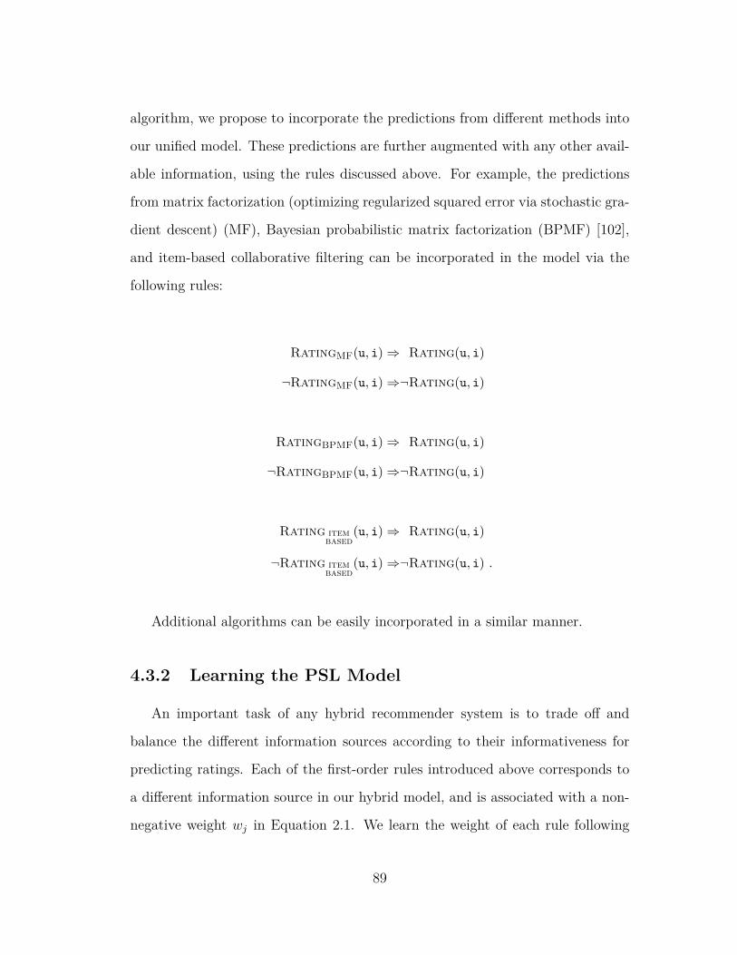
algorithm, we propose to incorporate the predictions from different methods into

our unified model. These predictions are further augmented with any other avail-

able information, using the rules discussed above. For example, the predictions

from matrix factorization (optimizing regularized squared error via stochastic gra-

dient descent) (MF), Bayesian probabilistic matrix factorization (BPMF) [102],

and item-based collaborative filtering can be incorporated in the model via the

following rules:

RatingMF(u, i)⇒ Rating(u, i)

¬RatingMF(u, i)⇒¬Rating(u, i)

RatingBPMF(u, i)⇒ Rating(u, i)

¬RatingBPMF(u, i)⇒¬Rating(u, i)

Rating itembased

(u, i)⇒ Rating(u, i)

¬Rating itembased

(u, i)⇒¬Rating(u, i) .

Additional algorithms can be easily incorporated in a similar manner.

4.3.2 Learning the PSL Model

An important task of any hybrid recommender system is to trade off and

balance the different information sources according to their informativeness for

predicting ratings. Each of the first-order rules introduced above corresponds to

a different information source in our hybrid model, and is associated with a non-

negative weight wj in Equation 2.1. We learn the weight of each rule following

89

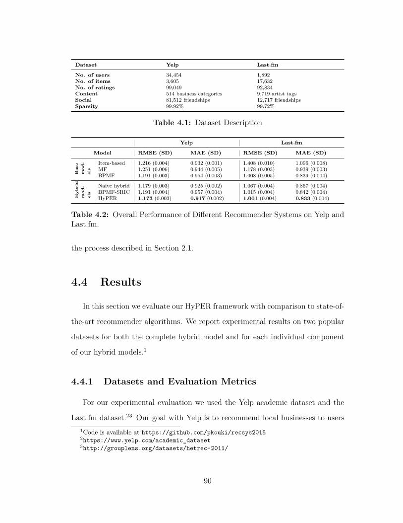
Dataset Yelp Last.fm

No. of users 34,454 1,892No. of items 3,605 17,632No. of ratings 99,049 92,834Content 514 business categories 9,719 artist tagsSocial 81,512 friendships 12,717 friendshipsSparsity 99.92% 99.72%

Table 4.1: Dataset Description

Yelp Last.fm

Model RMSE (SD) MAE (SD) RMSE (SD) MAE (SD)

Bas

em

od

-el

s

Item-based 1.216 (0.004) 0.932 (0.001) 1.408 (0.010) 1.096 (0.008)MF 1.251 (0.006) 0.944 (0.005) 1.178 (0.003) 0.939 (0.003)BPMF 1.191 (0.003) 0.954 (0.003) 1.008 (0.005) 0.839 (0.004)

Hy

bri

dm

od

-el

s

Naive hybrid 1.179 (0.003) 0.925 (0.002) 1.067 (0.004) 0.857 (0.004)BPMF-SRIC 1.191 (0.004) 0.957 (0.004) 1.015 (0.004) 0.842 (0.004)HyPER 1.173 (0.003) 0.917 (0.002) 1.001 (0.004) 0.833 (0.004)

Table 4.2: Overall Performance of Different Recommender Systems on Yelp andLast.fm.

the process described in Section 2.1.

4.4 Results

In this section we evaluate our HyPER framework with comparison to state-of-

the-art recommender algorithms. We report experimental results on two popular

datasets for both the complete hybrid model and for each individual component

of our hybrid models.1

4.4.1 Datasets and Evaluation Metrics

For our experimental evaluation we used the Yelp academic dataset and the

Last.fm dataset.23 Our goal with Yelp is to recommend local businesses to users1Code is available at https://github.com/pkouki/recsys20152https://www.yelp.com/academic_dataset3http://grouplens.org/datasets/hetrec-2011/

90

by predicting the missing ratings of businesses based on previous ratings. For our

experiments, we used all businesses, users, and ratings from Scottsdale, Arizona,

one of the largest cities in the dataset. Since we employ user and item similarities

as well as social information, it makes sense to focus those relationships within

the subgroup of the businesses of one physical location. Additionally, we used the

categories of each business as content information and the explicit user friendships

provided as social information. Yelp users give ratings from 1 to 5 stars, which

we linearly scaled into the [0,1] range that PSL operates over for the purposes of

our model.

For the Last.fm dataset our goal is to recommend artists to users. As Last.fm

does not provide explicit user-artist ratings we leverage the number of times a user

has listened to an artist to construct implicit ratings. We use a simple model-

based approach, where the repeated-listen counts for each user across artists are

modeled with a negative-binomial distribution. We used this distribution as it is

appropriate for count data where the sample variance is greater than the sample

mean, which is typically the case for Last.fm. For each user, we fit a negative

binomial to their counts via maximum likelihood estimation, and we calculate

the user’s implicit rating for an artist as the cumulative distribution function

(CDF) of the distribution, evaluated at the artist’s count. This corresponds to

the proportion of hypothetical artists that a user would listen to less than the

given artist, under the model. The Last.fm dataset also includes tags on artists

that we use for content-based information, as well as user friendship data that we

use for social recommendation.

We deliberately selected two datasets with a similar total number of ratings

but a different ratio of users to items. Different recommendation methods may

perform better with more users than items or vice versa, and hybrid systems

91

must account for this. We provide the summary statistics of the two datasets in

Table 4.1.

To learn the appropriate balance between information

sources for HyPER, i.e. to learn the weights of each rule in the model, we train

using the approximate maximum likelihood method described in Section 4.3.2,

with 20% of the training folds treated as the prediction target variables Y. Dur-

ing testing, we performed MAP inference to make predictions using ADMM. We

report the root mean squared error (RMSE) and the mean absolute error (MAE).

We compute these metrics by performing 5-fold cross-validation and reporting the

average cross-validated error.

4.4.2 Experimental Results

We report overall results with comparison to a selection of competing algo-

rithms in Table 4.2, and show more detailed results for the individual components

of our hybrid models in Tables 4.3 and 4.4. The following sections discuss these

results.

Overall Performance Comparison

We study the performance of HyPER in comparison to several state-of-the-art

models. We considered the following baselines:

• Item-based: The method in Equation 4.16 from [27], using Pearson’s cor-

relation with a mean-centering correction, as implemented in Graphlab.4

• Matrix factorization (MF): MF optimizing for regularized squared error

using stochastic gradient descent [64], as implemented in Graphlab.4http://www.dato.com

92

• Bayesian probabilistic matrix factorization

(BPMF): The Bayesian variant of probabilistic matrix factorization, trained

using Gibbs sampling [102].

• Naive hybrid: A simple hybrid approach where the predictions of the

above models are averaged.

• BPMF with social relations and items’ content (BPMF-SRIC): A

hybrid model that extends BPMF with social and content information [75].

The performance of our model is statistically significantly better than the

baselines at α = 0.05 for both datasets and evaluation metrics when using paired

t-test. We denote with bold the numbers that are statistically significantly better.

These results confirm our initial intuition that by incorporating a wide variety of

information sources and balancing them appropriately, the HyPER framework

manages to perform very well with rich and diverse datasets. We explore HyPER

components in more detail in the following section.

Performance per Information Type

For each type of information, we further evaluated our approach by building

simple HyPER models with each rule individually, and comparing these to com-

bined hybrid sub-models comprising all of the corresponding rules of that type.

Each sub-model also included the corresponding mean-centering rules (e.g. the

user-average rating rule for the user-based models). To balance the effect of each

rule, we performed weight learning within each training fold to learn rule weights.

We report the results for the Yelp dataset in Table 4.3 and for the last.fm dataset

in Table 4.4. The results show that for each information type, the HyPER model

which combines all of the corresponding components performs significantly better

93

than each component, considered in isolation. We denote with bold the cases

where the performance of each HyPER model is statistically significantly better

than all the individual models in the same category at α = 0.05 using paired

t-test. The final HyPER model shown in the last line, which combines all of

the available information into a single hybrid model, also performs statistically

significantly better than all sub-models and baselines.

Mean-Centering Priors: We created simple HyPER models using only the

average rating of each user, or the average rating of each item, or the average

overall rating, as well as a combined model. In the case of Yelp, the item-average

model had a lower error compared to the user average rule, while the opposite

was true for Last.fm (Tables 4.3(a) and 4.4(a)). This may be because the ratio

of users to items is different in the two datasets. The combined model performed

better than the individual models in both datasets.

Neighborhood-Based Collaborative Filtering: We constructed individ-

ual models based on the similarities described in Section 4.3.1. The number

of neighbors is typically set to between 20 and 50 in the literature [27], and so

we used 50 neighbors for users/item in all experiments. We also employed

a mean-centered approach by providing each of these models with the corre-

sponding average-rating mean-centering rules (e.g. the average user-rating rule

for user-based collaborative filtering). As in the previous experiment, user-based

techniques perform poorly on Yelp, but have better performance on Last.fm (Ta-

bles 4.3(b), 4.4(b) and 4.3(c), 4.4(c)). The opposite is true for the item-based

techniques, which perform poorly on Last.fm, but better on Yelp. The perfor-

mance varied between the different similarity measures, with distances computed

in the latent space usually performing the best individually. Again, the HyPER

combination of all similarity measures improves performance.

94

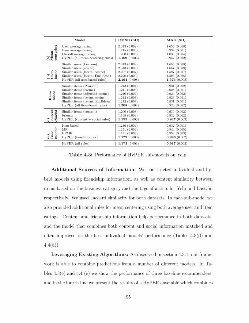
Model RMSE (SD) MAE (SD)

(a)

Mea

n-ce

nter

ing User average rating 2.313 (0.008) 1.656 (0.008)

Item average rating 1.215 (0.003) 0.932 (0.001)Overall average rating 1.280 (0.005) 1.030 (0.004)HyPER (all mean-centering rules) 1.199 (0.003) 0.952 (0.002)

(b)

Use

r-ba

sed

Similar users (Pearson) 2.313 (0.008) 1.656 (0.008)Similar users (cosine) 2.313 (0.008) 1.657 (0.008)Similar users (latent, cosine) 2.227 (0.007) 1.597 (0.007)Similar users (latent, Euclidean) 2.226 (0.009) 1.596 (0.008)HyPER (all user-based rules) 2.194 (0.008) 1.573 (0.008)

Item

-ba

sed

Similar items (Pearson) 1.213 (0.004) 0.931 (0.002)Similar items (cosine) 1.211 (0.003) 0.928 (0.001)Similar items (adjusted cosine) 1.210 (0.004) 0.924 (0.002)Similar items (latent, cosine) 1.212 (0.003) 0.923 (0.001)Similar items (latent, Euclidean) 1.212 (0.003) 0.931 (0.001)HyPER (all item-based rules) 1.208 (0.004) 0.923 (0.002)

(d)

Con

tent

&So

cial Similar items (content) 1.200 (0.003) 0.939 (0.002)

Friends 1.199 (0.003) 0.932 (0.002)HyPER (content + social rules) 1.195 (0.003) 0.927 (0.002)

(e)

Bas

em

odel

s Item-based 1.216 (0.004) 0.932 (0.001)MF 1.251 (0.006) 0.944 (0.005)BPMF 1.191 (0.003) 0.954 (0.003)HyPER (baseline rules) 1.179 (0.003) 0.926 (0.002)

HyPER (all rules) 1.173 (0.003) 0.917 (0.002)

Table 4.3: Performance of HyPER sub-models on Yelp.

Additional Sources of Information: We constructed individual and hy-

brid models using friendship information, as well as content similarity between

items based on the business category and the tags of artists for Yelp and Last.fm

respectively. We used Jaccard similarity for both datasets. In each sub-model we

also provided additional rules for mean centering using both average user and item

ratings. Content and friendship information help performance in both datasets,

and the model that combines both content and social information matched and

often improved on the best individual models’ performance (Tables 4.3(d) and

4.4(d)).

Leveraging Existing Algorithms: As discussed in section 4.3.1, our frame-

work is able to combine predictions from a number of different models. In Ta-

bles 4.3(e) and 4.4 (e) we show the performance of three baseline recommenders,

and in the fourth line we present the results of a HyPER ensemble which combines

95

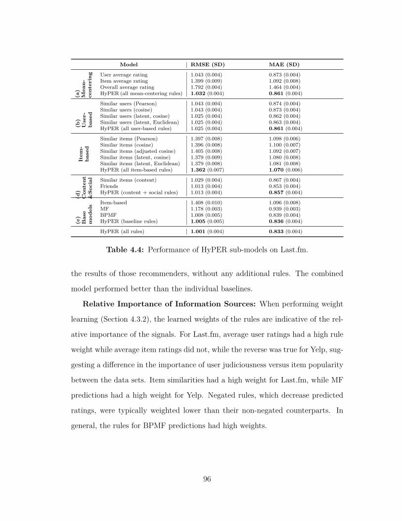
Model RMSE (SD) MAE (SD)

(a)

Mea

n-ce

nter

ing User average rating 1.043 (0.004) 0.873 (0.004)

Item average rating 1.399 (0.009) 1.092 (0.008)Overall average rating 1.792 (0.004) 1.464 (0.004)HyPER (all mean-centering rules) 1.032 (0.004) 0.861 (0.004)

(b)

Use

r-ba

sed

Similar users (Pearson) 1.043 (0.004) 0.874 (0.004)Similar users (cosine) 1.043 (0.004) 0.873 (0.004)Similar users (latent, cosine) 1.025 (0.004) 0.862 (0.004)Similar users (latent, Euclidean) 1.025 (0.004) 0.863 (0.004)HyPER (all user-based rules) 1.025 (0.004) 0.861 (0.004)

Item

-ba

sed

Similar items (Pearson) 1.397 (0.008) 1.098 (0.006)Similar items (cosine) 1.396 (0.008) 1.100 (0.007)Similar items (adjusted cosine) 1.405 (0.008) 1.092 (0.007)Similar items (latent, cosine) 1.379 (0.009) 1.080 (0.008)Similar items (latent, Euclidean) 1.379 (0.008) 1.081 (0.008)HyPER (all item-based rules) 1.362 (0.007) 1.070 (0.006)

(d)

Con

tent

&So

cial Similar items (content) 1.029 (0.004) 0.867 (0.004)

Friends 1.013 (0.004) 0.853 (0.004)HyPER (content + social rules) 1.013 (0.004) 0.857 (0.004)

(e)

Bas

em

odel

s Item-based 1.408 (0.010) 1.096 (0.008)MF 1.178 (0.003) 0.939 (0.003)BPMF 1.008 (0.005) 0.839 (0.004)HyPER (baseline rules) 1.005 (0.005) 0.836 (0.004)

HyPER (all rules) 1.001 (0.004) 0.833 (0.004)

Table 4.4: Performance of HyPER sub-models on Last.fm.

the results of those recommenders, without any additional rules. The combined

model performed better than the individual baselines.

Relative Importance of Information Sources: When performing weight

learning (Section 4.3.2), the learned weights of the rules are indicative of the rel-

ative importance of the signals. For Last.fm, average user ratings had a high rule

weight while average item ratings did not, while the reverse was true for Yelp, sug-

gesting a difference in the importance of user judiciousness versus item popularity

between the data sets. Item similarities had a high weight for Last.fm, while MF

predictions had a high weight for Yelp. Negated rules, which decrease predicted

ratings, were typically weighted lower than their non-negated counterparts. In

general, the rules for BPMF predictions had high weights.

96

4.5 Conclusions and Future Work

In this Chapter we presented HyPER, a new hybrid recommender system

which is flexible, problem-agnostic, and is easily extensible via a probabilistic pro-

gramming interface. HyPER uses a hinge-loss MRF formulation, allowing scal-

able and accurate inference. Our comprehensive experiments demonstrate that

HyPER can learn to appropriately balance many information sources, resulting

in improved performance over previous state-of-the-art approaches on two bench-

mark datasets.

In our future work we plan to extend our model to account for knowledge

coming from ontologies as well as temporal signals. Finally, the current evalua-

tion shows that our model outperforms state-of-the-art algorithms for the rating

prediction task. In the future, we would like to evaluate the performance of our

model in the ranking task and compare it with state-of-the-art algorithms such as

Bayesian Personalized Ranking [99].

97

Chapter 5

Explanations in Richly

Structured Social Networks

A driving force behind recent improvements in recommender systems are frame-

works that combine information from diverse sources such as social connections,

collaborative filtering (CF) approaches, and item metadata to provide better rec-

ommendations. These “hybrid” recommender systems have proven effective in

making state-of-the-art recommendations, but their benefits have come at the cost

of increased complexity and opacity. As recommendations have become central to

combating information overload and shaping decisions, users increasingly demand

convincing explanations to help them understand why particular recommenda-

tions are made [11, 86]. In this Chapter, we develop a framework for providing

real-time, personalized explanations from hybrid recommenders and perform two

real-world user studies to better understand which explanations and visualizations

are the most convincing.

The majority of literature on explaining recommendations [52, 10, 107, 116,

20] has focused on studying explanations from non-hybrid (single-source) recom-

mender systems. Typically, explanations from single-source recommenders come

98

in a single style, e.g., a content-based recommender system produces content-based

explanations. Existing work has explored user preferences for these single-style

explanations [52, 10]. Visualization techniques for explaining recommendations

include interfaces with concentric circles [87, 59], Venn diagrams [91], and path-

ways between columns [11], among many others. A recent survey [90] of different

single-style explanation approaches has concluded that hybrid explanations, which

combine multiple styles, such as user-based and item-based, are more effective than

non-hybrid counterparts. Despite these findings, there has been no comprehen-

sive study to determine the best methods for presenting recommendations while

taking into account user preferences for hybrid explanations.

In this Chapter, we use the basic design principles described in Chapter 4 to

build a music recommender system capable of incorporating any number of infor-

mation sources. Then, we extend this system to provide explanations that vary

in style, volume (i.e., number of explanation styles), and visualization format.

Finally, we conduct two large user studies, a non-personalized and a personalized

one. In the first, non-personalized study, users evaluate several different design

approaches (e.g., textual, visual) for hybrid explanations. This general evaluation

strategy can be used to study user preferences for different recommendation do-

mains, such as career sites, music services, and navigational routes. To the best

of our knowledge, this is the first study that adapts visualization techniques to

hybrid recommenders and compares user preferences for hybrid explanations. We

use the findings from the first study and perform a second personalized one, where

we provide real users of a social media site personalized recommendations with

hybrid explanations. Our goal is to understand how different variables (style, vol-

ume, format) impact the subjective persuasiveness of recommendations. Recent

research [8] has indicated that there may be a relationship between a person’s

99

personality and the type of explanation that is most persuasive, so we also conduct

an exploratory analysis for hybrid explanations. To the best of our knowledge, our

work is the first comprehensive study of the effect of such variables on personalized

hybrid explanations.

In more detail, in the first part of our work, we extend HyPER introduced in

Chapter 4, to produce real-time recommendations while incorporating a variety

of information sources. We build a real-time data collection system for acquiring

a user’s history, social connections, tags, and popularity statistics from a social

media site. We use these signals to create a hybrid model similar to the model

described in Chapter 4 that incorporates user-user and item-item similarities using

CF, content, social, and popularity information. Next, we implement a parser that

generates customized explanations from the output of the hybrid system in real

time. We support several different explanation styles, including user-based, item-

based, content, social, and item popularity. Table 5.1 shows an example of a

recommendation along with the explanations generated by our framework.

In the second part of our work, we study the effect of different explanation

presentation styles on user experience. To this end, we identify several dimensions

for designing interfaces. We conduct a crowd-sourced user study (N = 200) using

Amazon Mechanical Turk (AMT) where we show to the participants a set of dif-

ferent interfaces that provide recommendations along with hybrid explanations.

This study answers several fundamental questions about designing hybrid expla-

nations: 1) What visualization is best for hybrid explanations? 2) How should

explanations be organized? 3) How much information should be in each explana-

tion? 4) How detailed should each explanation be? Figure 5.1 presents a sample

of different visualizations that we generated in order to understand user prefer-

ences for hybrid explanations. Among different visualizations we find that Venn

100

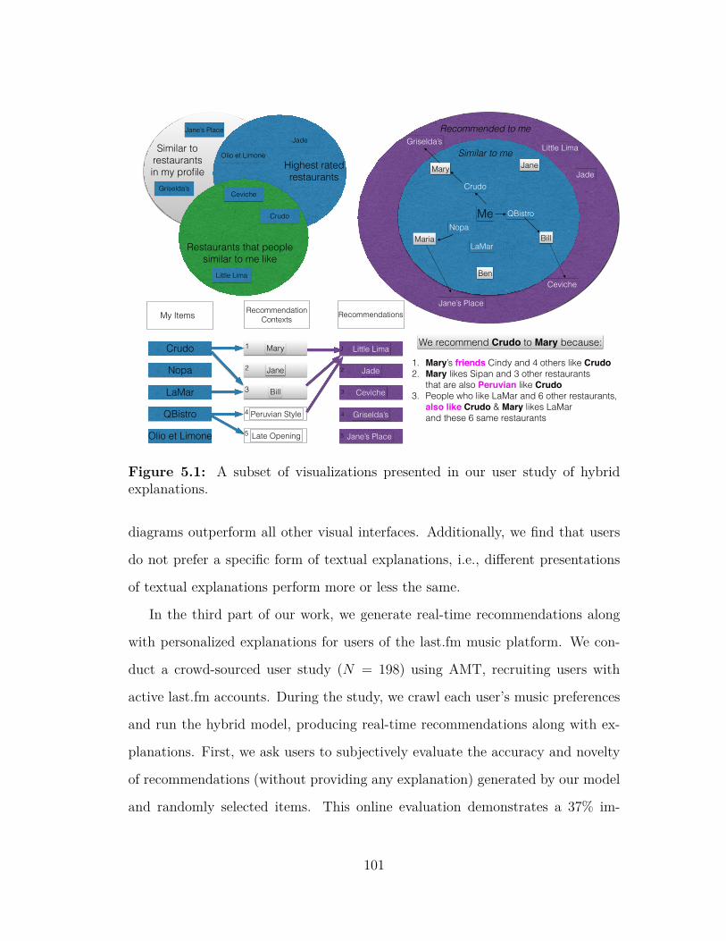
Me

Mary Jane

BillMaria

Ben

Little Lima

Jade

Ceviche

Griselda’s

Jane’s Place

Crudo

Nopa

LaMar

QBistro

Similar to me

Recommended to me

Similar to restaurants in my profile Highest rated

restaurants

Restaurants that people similar to me like

Ceviche

Crudo

Jade

Little Lima

Griselda’s

Olio et Limone

Jane’s Place

Crudo

Nopa

LaMar

QBistro

Olio et Limone

Mary

Jane

Bill

Peruvian Style

Little Lima

Jade

Ceviche

Griselda’s

Late Opening Jane’s Place

My Items Recommendation Contexts Recommendations

1

2

3

5

4

1

2

3

5

4

We recommend Crudo to Mary because:

1. Mary’s friends Cindy and 4 others like Crudo 2. Mary likes Sipan and 3 other restaurants

that are also Peruvian like Crudo 3. People who like LaMar and 6 other restaurants,

also like Crudo & Mary likes LaMar and these 6 same restaurants

Figure 5.1: A subset of visualizations presented in our user study of hybridexplanations.

diagrams outperform all other visual interfaces. Additionally, we find that users

do not prefer a specific form of textual explanations, i.e., different presentations

of textual explanations perform more or less the same.

In the third part of our work, we generate real-time recommendations along

with personalized explanations for users of the last.fm music platform. We con-

duct a crowd-sourced user study (N = 198) using AMT, recruiting users with

active last.fm accounts. During the study, we crawl each user’s music preferences

and run the hybrid model, producing real-time recommendations along with ex-

planations. First, we ask users to subjectively evaluate the accuracy and novelty

of recommendations (without providing any explanation) generated by our model

and randomly selected items. This online evaluation demonstrates a 37% im-

101

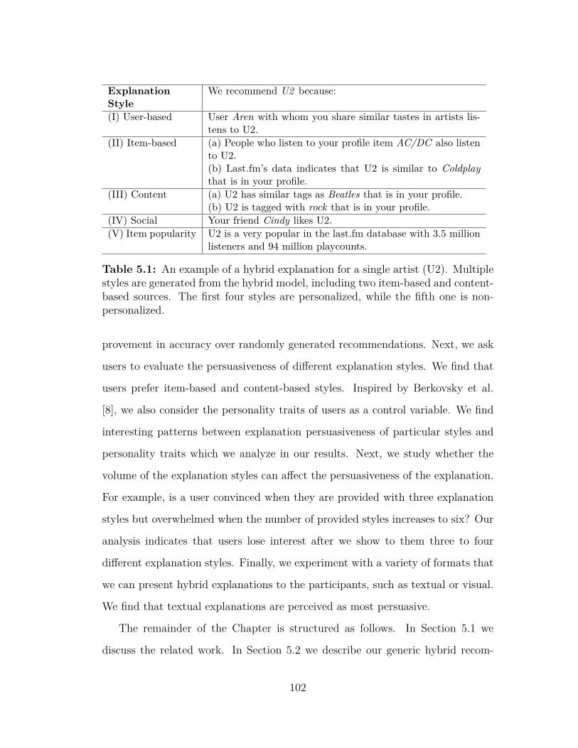
ExplanationStyle

We recommend U2 because:

(I) User-based User Aren with whom you share similar tastes in artists lis-tens to U2.

(II) Item-based (a) People who listen to your profile item AC/DC also listento U2.(b) Last.fm’s data indicates that U2 is similar to Coldplaythat is in your profile.

(III) Content (a) U2 has similar tags as Beatles that is in your profile.(b) U2 is tagged with rock that is in your profile.

(IV) Social Your friend Cindy likes U2.(V) Item popularity U2 is a very popular in the last.fm database with 3.5 million

listeners and 94 million playcounts.

Table 5.1: An example of a hybrid explanation for a single artist (U2). Multiplestyles are generated from the hybrid model, including two item-based and content-based sources. The first four styles are personalized, while the fifth one is non-personalized.

provement in accuracy over randomly generated recommendations. Next, we ask

users to evaluate the persuasiveness of different explanation styles. We find that

users prefer item-based and content-based styles. Inspired by Berkovsky et al.

[8], we also consider the personality traits of users as a control variable. We find

interesting patterns between explanation persuasiveness of particular styles and

personality traits which we analyze in our results. Next, we study whether the

volume of the explanation styles can affect the persuasiveness of the explanation.

For example, is a user convinced when they are provided with three explanation

styles but overwhelmed when the number of provided styles increases to six? Our

analysis indicates that users lose interest after we show to them three to four

different explanation styles. Finally, we experiment with a variety of formats that

we can present hybrid explanations to the participants, such as textual or visual.

We find that textual explanations are perceived as most persuasive.

The remainder of the Chapter is structured as follows. In Section 5.1 we

discuss the related work. In Section 5.2 we describe our generic hybrid recom-

102

mendation framework. For the purpose of this Chapter, we use the music domain

as an example and specifically data and users from last.fm. Our framework uses

the basic design principles described in Chapter 4. In Sections 5.3 and 5.4 we

describe in detail the non-personalized and personalized user studies, the research

questions, and our results. Finally, in Section 5.5 we report the basic conclusions

and describe our future work plans.

5.1 Related Work

We organize our discussion of previous studies on explanations for recom-

mender systems along three themes: i) work on single-style explanations, ii) work

combining more than one explanation style and, iii) work surveying the state-of-

the-art in explanations for decision support and recommender systems.

Single-Style Explanations. Herlocker et al. [52] show that certain explanation

and presentation styles can increase a recommender system’s effectiveness in con-

vincing users to make a purchase. Bilgic and Mooney [10] compare single-style

explanations that use content-based keywords, item-based CF, or prior rating his-

tory. Vig et al. [116] show that explanations using tags improve effectiveness.

Tintarev and Masthoff [109] found that, despite improving user satisfaction, per-

sonalization can reduce the effectiveness of content-based explanations. Recently,

Oramas et al. [89] built a music knowledge base and generated content-based

natural language explanations. They found that the effectiveness of an explana-

tion depends on the familiarity with recommender systems and the users’ music

education. PeerChooser [87] provides user-based CF explanations through an in-

teractive graphical interface in the form of concentric circles. Berkovsky et al. [8]

study the effect of three different explanation styles (item-based, average rating,

and popularity-based) on user trust considering the users’ personality traits as a

103

control variable. Inspired by this work, we study whether varying the explanation

style or volume changes the persuasiveness of explanations when controlling for

different personality traits.

Hybrid Explanations. Most research on hybrid explanations focuses on propos-

ing graphical interfaces to visualize the different explanation styles. TalkEx-

plorer [115] combines content, tag, and social-based filtering techniques to provide

an interactive interface in the form of clustermaps. SetFusion [91] builds on Talk-

Explorer and replaces clustermaps with Venn diagrams showing improved user

experience. TasteWeights [11] builds an interactive hybrid recommender system

that combines social, content, and expert information. The framework shows the

reasoning behind the recommendations in the form of pathways among columns.

Nguyen et al. [83] aim to reduce the noise in user ratings by proposing interfaces

that support explanations in the form of tags, exemplars, and their combination.

Symeonidis et al. [107] combine content-based filtering and rating history to gen-

erate natural language explanations which are all of the same type. Finally, Kouki

et al. [69] manually generate hybrid explanations in a restaurant recommendation

setting. The authors conduct a synthetic user study where participants evaluate

non-personalized explanations that were manually produced. In this Chapter, we

implement a hybrid recommender system which automatically generates recom-

mendations together with explanations, building on a system called HyPER [65].

We use this system to generate personalized, real-time recommendations with ex-

planations for active users of a music platform. In our personalized user study we

analyze both the recommendation quality and the explanation persuasiveness by

varying several different variables.

Surveys on Explanations. Nunes and Jannach [86] review the literature on

explanations in decision-support systems. The authors distinguish variables such

104

as the length of the explanation, its vocabulary, and the presentation of the expla-

nation and conclude that additional studies are necessary to assess the impact of

these variables. One of the goals of our work is to determine whether the explana-

tion length and its presentation affect user satisfaction. Friedrich and Zanker [39]

propose a taxonomy that categorizes different explainable recommender systems.

The authors argue that future research should create new kinds of information,

interaction, and presentation styles and also analyze how, and under what condi-

tions, these will affect different explanation objectives. To this end, we offer seven

different explanation styles and study their effect on persuasiveness when taking

different variables into account.

To summarize, our work differs from prior art in the following ways:

• Several general user interfaces (GUIs) and visualizations have been proposed

for recommendations, including concentric circles (PeerChooser [87, 59]),

clustermaps (TalkExplorer [115]), Venn diagrams (SetFusion [91]), and paths

among columns (TasteWeights [11, 60]). Extending these ideas, we focus on

hybrid explanations and study user preferences across designs and interfaces.

• Existing work proposing explanations either does not involve a recommen-

dation algorithm [8], or uses a baseline recommender [11, 89]. In our case, we

show how to generate explanations from the HyPER recommender system

that has showed improved performance over the state-of-the-art. Addition-

ally, we evaluate the accuracy of our framework in an online setting over

real data. Our work considers seven different explanation styles, while most

of prior work considers up to three explanation styles. To the best of our

knowledge, our personalized user study is the first one analyzing the effect of

different personalized explanation styles, their volume, and format on per-

suasiveness. Finally, our personalized study is the first that considers the

105

users’ personality traits as a control variable.

5.2 Explainable Hybrid Recommender

In this section, we describe how we use the hybrid recommender system (Hy-

PER) presented in Chapter 4 to generate explainable recommendations. We first

describe how we use HyPER to implement a music recommender system (which

we call HyPER-music) and then we discuss how we transform the model’s proba-

bilistic factors to explanations capturing the different recommender signal types.

5.2.1 Hybrid Music Recommender Model

As we saw, HyPER provides a generic and extensible recommendation frame-

work with the ability to incorporate any other sources of information that are

available in any custom dataset or application scenario. In this chapter, we focus

on music recommendations. We use a subset of all the rules proposed in HyPER

and, given its extensibility, we add several rules to leverage dataset-specific infor-

mation available in our music dataset. We propose a hybrid music-recommender

system, called HyPER-music, which consists of the following rules:

106

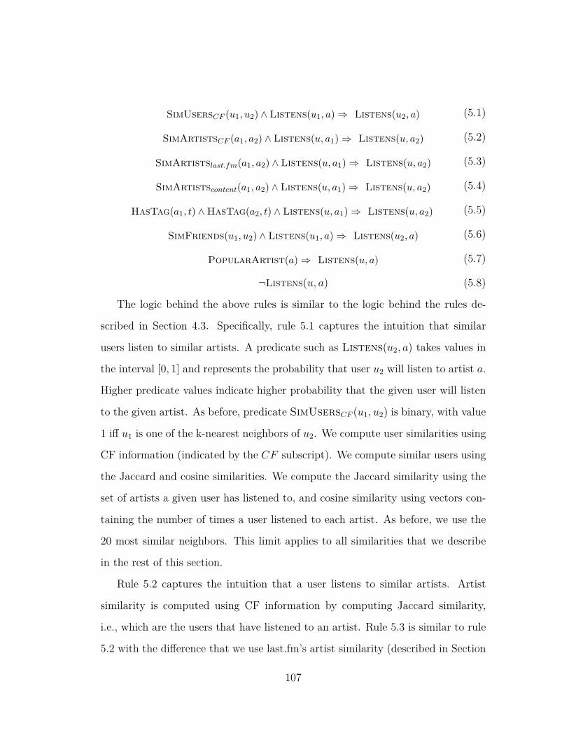
SimUsersCF (u1, u2) ∧ Listens(u1, a)⇒ Listens(u2, a) (5.1)

SimArtistsCF (a1, a2) ∧ Listens(u, a1)⇒ Listens(u, a2) (5.2)

SimArtistslast.fm(a1, a2) ∧ Listens(u, a1)⇒ Listens(u, a2) (5.3)

SimArtistscontent(a1, a2) ∧ Listens(u, a1)⇒ Listens(u, a2) (5.4)

HasTag(a1, t) ∧HasTag(a2, t) ∧ Listens(u, a1)⇒ Listens(u, a2) (5.5)

SimFriends(u1, u2) ∧ Listens(u1, a)⇒ Listens(u2, a) (5.6)

PopularArtist(a)⇒ Listens(u, a) (5.7)

¬Listens(u, a) (5.8)

The logic behind the above rules is similar to the logic behind the rules de-

scribed in Section 4.3. Specifically, rule 5.1 captures the intuition that similar

users listen to similar artists. A predicate such as Listens(u2, a) takes values in

the interval [0, 1] and represents the probability that user u2 will listen to artist a.

Higher predicate values indicate higher probability that the given user will listen

to the given artist. As before, predicate SimUsersCF (u1, u2) is binary, with value

1 iff u1 is one of the k-nearest neighbors of u2. We compute user similarities using

CF information (indicated by the CF subscript). We compute similar users using

the Jaccard and cosine similarities. We compute the Jaccard similarity using the

set of artists a given user has listened to, and cosine similarity using vectors con-

taining the number of times a user listened to each artist. As before, we use the

20 most similar neighbors. This limit applies to all similarities that we describe

in the rest of this section.

Rule 5.2 captures the intuition that a user listens to similar artists. Artist

similarity is computed using CF information by computing Jaccard similarity,

i.e., which are the users that have listened to an artist. Rule 5.3 is similar to rule

5.2 with the difference that we use last.fm’s artist similarity (described in Section

107

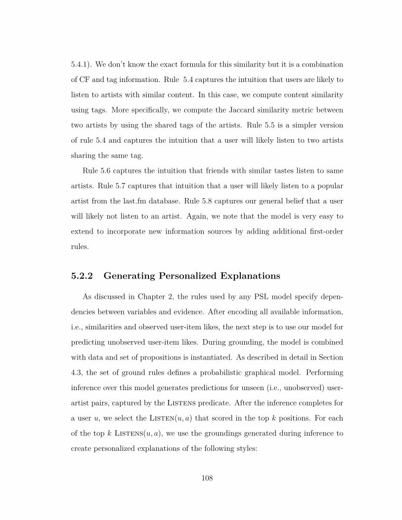
5.4.1). We don’t know the exact formula for this similarity but it is a combination

of CF and tag information. Rule 5.4 captures the intuition that users are likely to

listen to artists with similar content. In this case, we compute content similarity

using tags. More specifically, we compute the Jaccard similarity metric between

two artists by using the shared tags of the artists. Rule 5.5 is a simpler version

of rule 5.4 and captures the intuition that a user will likely listen to two artists

sharing the same tag.

Rule 5.6 captures the intuition that friends with similar tastes listen to same

artists. Rule 5.7 captures that intuition that a user will likely listen to a popular

artist from the last.fm database. Rule 5.8 captures our general belief that a user

will likely not listen to an artist. Again, we note that the model is very easy to

extend to incorporate new information sources by adding additional first-order

rules.

5.2.2 Generating Personalized Explanations

As discussed in Chapter 2, the rules used by any PSL model specify depen-

dencies between variables and evidence. After encoding all available information,

i.e., similarities and observed user-item likes, the next step is to use our model for

predicting unobserved user-item likes. During grounding, the model is combined

with data and set of propositions is instantiated. As described in detail in Section

4.3, the set of ground rules defines a probabilistic graphical model. Performing

inference over this model generates predictions for unseen (i.e., unobserved) user-

artist pairs, captured by the Listens predicate. After the inference completes for

a user u, we select the Listen(u, a) that scored in the top k positions. For each

of the top k Listens(u, a), we use the groundings generated during inference to

create personalized explanations of the following styles:

108

• User-based, with explanations similar to the example of Table 5.1(I) using

the groundings of rule 5.1.

• Item-based CF and item-based last.fm, with explanations similar to

Table Table5.1(II-a, II-b), using the groundings of rules 5.2 and 5.3 respec-

tively.

• Content-based Jaccard and content-based tags, with explanations sim-

ilar to Table 5.1(III-a, III-b) using the groundings of rules 5.4 and 5.5 re-

spectively.

• Social-based, with explanations similar to Table 5.1(IV) using the ground-

ings of rule 5.6.

• Popularity-based, with explanations similar to Table 5.1(V) using the

groundings of rule 5.7.

As an example, let’s assume that for user Jen, the predicted value of the

unobserved variable Listens(Jen, U2) has the highest value among all other pre-

dicted values and, during inference, the following ground rules associated with

Listens(Jen, U2) were generated:

SimUsersCF (Jen, Aren) ∧ Listens(Aren, U2) ⇒ Listens(Jen, U2)

SimArtistsCF (U2, ACDC) ∧ Listens(Jen, ACDC) ⇒ Listens(Jen, U2)

SimArtistslast.fm(U2, Coldplay) ∧ Listens(Jen, Coldplay) ⇒ Listens(Jen, U2)

SimArtistscontent(U2, Beatles) ∧ Listens(Jen, Beatles) ⇒ Listens(Jen, U2)

HasTag(U2, Rock) ∧ HasTag(Slayer, Rock) ∧ Listens(Jen, Slayer) ⇒ Listens(Jen, U2)

SimFriends(Jen, Cindy) ∧ Listens(Cindy, U2) ⇒ Listens(Jen, U2)

PopularArtist(U2) ⇒ Listens(Jen, U2)

In order to generate explanations from the ground rules, we develop a parser

that takes as input the groundings and outputs sentences in natural language.

109

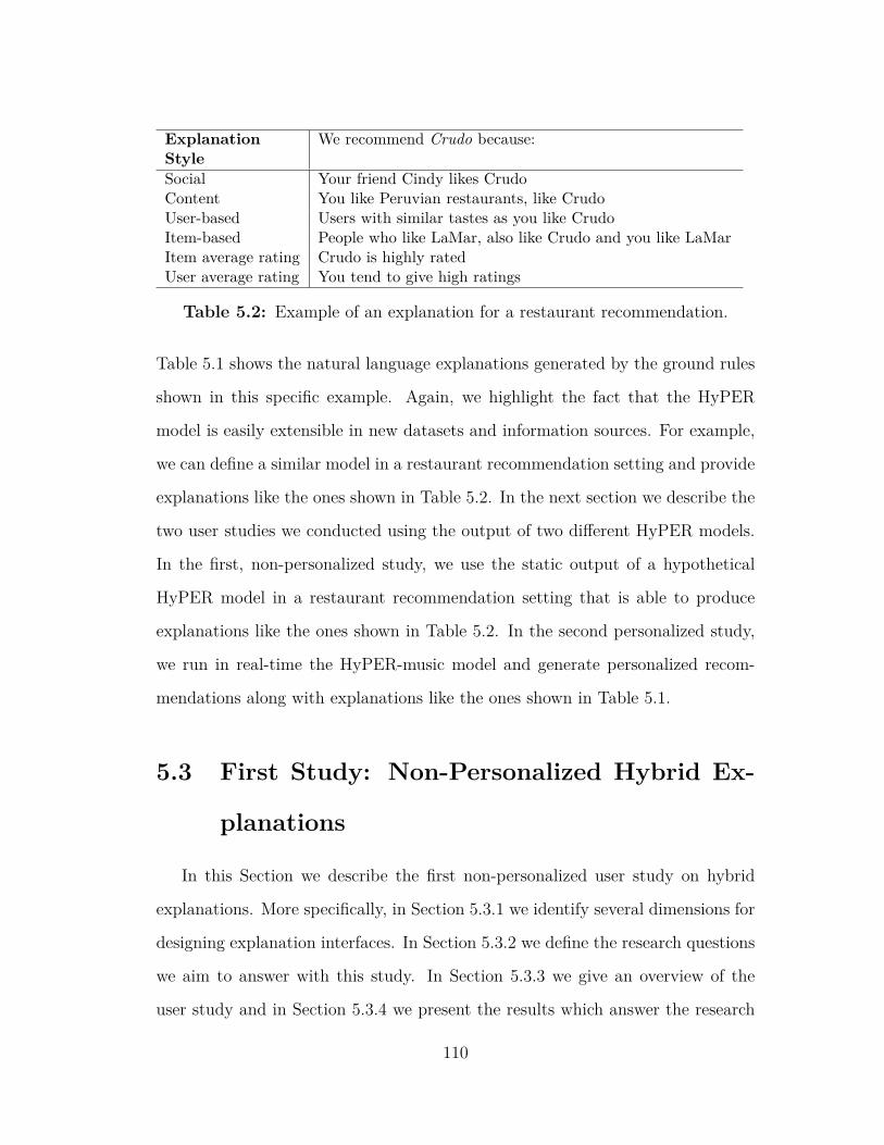
ExplanationStyle

We recommend Crudo because:

Social Your friend Cindy likes CrudoContent You like Peruvian restaurants, like CrudoUser-based Users with similar tastes as you like CrudoItem-based People who like LaMar, also like Crudo and you like LaMarItem average rating Crudo is highly ratedUser average rating You tend to give high ratings

Table 5.2: Example of an explanation for a restaurant recommendation.

Table 5.1 shows the natural language explanations generated by the ground rules

shown in this specific example. Again, we highlight the fact that the HyPER

model is easily extensible in new datasets and information sources. For example,

we can define a similar model in a restaurant recommendation setting and provide

explanations like the ones shown in Table 5.2. In the next section we describe the

two user studies we conducted using the output of two different HyPER models.

In the first, non-personalized study, we use the static output of a hypothetical

HyPER model in a restaurant recommendation setting that is able to produce

explanations like the ones shown in Table 5.2. In the second personalized study,

we run in real-time the HyPER-music model and generate personalized recom-

mendations along with explanations like the ones shown in Table 5.1.

5.3 First Study: Non-Personalized Hybrid Ex-

planations

In this Section we describe the first non-personalized user study on hybrid

explanations. More specifically, in Section 5.3.1 we identify several dimensions for

designing explanation interfaces. In Section 5.3.2 we define the research questions

we aim to answer with this study. In Section 5.3.3 we give an overview of the

user study and in Section 5.3.4 we present the results which answer the research

110

questions. Finally, in Section 5.3.5 we summarize our findings.

5.3.1 Presentation of Explanations

In this study, we assume that we are given the output of a hypothetical Hy-

PER model in a restaurant recommendation setting, that produces explanations

like the ones in Table 5.2. The next step is designing an interface to present

these explanations to users. At a high level, the goal of any presentation style is

to improve the user experience. We study the effect of different explanation pre-

sentation styles on user experience. To this end, we identify several dimensions

for designing interfaces:

• Presentation (Pres.): Natural language (Table 5.2), rule-based, or graph-

ical visualizations.

• Weighting (Wgt): Whether or not explanation weights are displayed. As

we discussed, HyPER supports a weight learning mechanism that automati-

cally learns to balance the different information signals (e.g. social, content)

when making predictions.

• Grouping (Group): Whether or not explanations are grouped by style.

Each rule can have many groundings in a dataset. For example, do users

prefer to be shown the explanation “Mary’s friend Cindy likes Crudo; Mary’s

friend Josh likes Crudo” or grouping explanations, “Mary’s friends Cindy

and Josh like Crudo.”?

• Information Density (Dens.): Amount of information shown. Should

explanations be high or low information? If there are many groundings for

each of the template rules, do users like to be shown all the groundings

111

or do they get overwhelmed and prefer to be shown a small subset of the

groundings?

• Aggregation (Aggr.): Whether or not rules are aggregated in the grouping

case. Do users prefer explanations of the type “Mary’s friends Cindy and 4

others like Crudo.” or “Mary’s friends Cindy, Josh, Rosie, George, Michael

like Crudo.”?

• Meta-explanations (Meta): Amount of high-level metadata in explana-

tions (i.e., user similarity, item average rating, and user average rating). Do

users prefer to see explanations that can be highly personalized or they see

a value in explanations that are general and not so easy to personalize? We

consider social, content, and item-based explanations easy to personalize

and user, item popularity, and user average rating not easy to personalize.

• Visualization (Visual): What is the best way to visualize hybrid expla-

nations? Literature has proposed different ways to visualize explanations.

We use these visualizations in a hybrid explanation setting and evaluate

which one users prefer. In particular, we check the performance of concen-

tric circles [87, 59], Venn diagrams [91], pathways among columns [11], and

one new approach that is based on pathways among columns that addition-

ally shows the reasoning behind each prediction. For Venn diagrams we

used only 3 intersections which has been shown to work well in the previous

literature [115].

In addition to the effect of different presentation styles on user experience,

we also studied whether users have a specific preference over the ranking of the

different explanation styles. For example, do users prefer to see social explanations

before content-based ones?

112

Treat. Pres. Wgt Group Dens. Aggr. MetaBASE no exp. no no NA no NAAGGR english no yes low yes lowGROUP english no yes high no lowRULE rule no no low no highWGT english yes no low no highPLAIN english no no low no highNO-GR english no no med no lowMED-IN english no yes med no lowLOW-IN english no yes low no low

Visual StyleCOL visual COLumns + pathwaysCPR visual Columns + Pathways with ReasoningVENN visual VENN diagramCC visual Concentric Circles

Table 5.3: Dimension values for each treatment for the different types of expla-nations tested.

5.3.2 Research Questions

The above dimensions help us define and answer the following four fundamental

questions about recommendations and explanations coming from a hybrid system:

1. What visualization is best for hybrid explanations?

2. How should explanations be organized?

3. How much information should be in each explanation?

4. How detailed should each explanation be?

5.3.3 Study Design

In this section, we describe our study from the point of view of one participant.

The study is divided in two phases. In the first phase, we ask the participant to

fill in a pre-questionnaire (this is the same for all participants). In the second part

of the study, we show a variety of mockups to the participants. We note that the

mockups are non-personalized and they are the same for all participants.

113

First Phase: Pre-study Questionnaire

The title of the study was “PSLViz! A new way to explore recommendation”

which was followed by a short description: “You are about to explore new ways to

find interesting items!” Afterwards, we asked the participant a set of demographic

questions (age range, gender, education level). We also asked users to indicate if

they have issues with color blindness. Next, we asked the participants questions

related to visualization familiarity (reported in lines 2-5 of Table 5.5). Responses

were provided using a 7-point Likert scale from “Totally Disagree” to “Totally

Agree”.

Second Phase: Main Study Questionnaire

In the second part of the study, interface mockups were shown to participants

in random order. We ran a synthetic experiment where all users were shown the

exact same mockups that were manually generated. Each mockup presented a

hybrid explanation for a random user called “Mary” for the restaurant “Crudo”.

For each mockup, we elicited answers for a set of user experience questions, corre-

sponding to understandability, system satisfaction, and perceived persuasiveness

(Table 5.5). Testing all possible subsets of dimensions was prohibitive, so we chose

subsets that we judged as the most informative for explanation design. We evalu-

ated explanations for a variety of textual and visual formats. We also included a

baseline treatment (BASE) where we presented a recommendation item without

any explanation. More specifically, we presented a total of 13 treatments to the

participants, 9 text-based (Figures 5.2- 5.9) and 4 visual-based (Figures 5.10 -

5.13). The treatment without the explanation (BASE) was “We recommend that

Mary likes Crudo”. Table 5.3 summarizes the dimension values for each treatment

for the different types of explanations tested. Here is a more detailed description

114

of the treatments:

• Treatment AGGR, (Figure 5.2) presents explanations in text format, does not

assign weights to explanations, groups different instantiations of the same rule in

one explanation sentence (e.g., we show one explanation that includes friends),

aggregates instances of the same rule in one explanation sentence (e.g., we

aggregate the friends in a number (4) and does not refer to the name of each

friend), the amount of information shown is low (e.g., we present the name of

only one friend), and takes into account only user preferences (and does not

include high-level explanations).

• Treatment GROUP (Figure 5.3) presents explanations in text format, does not

assign weights to explanations, groups different instantiations of the same rule in

one explanation sentence (e.g., we show one explanation that includes friends),

does not aggregate instances of the same rule in one explanation sentence (e.g.,

all friends are listed by their names), the amount of information shown is high

(e.g., we present 5 similar friends), and takes into account only user preferences.

• Treatment RULE (Figure 5.4) presents explanations in text, rule-based format,

does not assign weights to explanations, does not group different instantiations

of the same rule, does not aggregate instances of the same rule, the amount

of information shown is low, and takes into account both user preferences and

high-level metadata (e.g., user similarity).

• Treatment WGT (Figure 5.5) presents explanations in text format, does assign

weights to explanations, does not group different instantiations of the same rule,

does not aggregate instances of the same rule, the amount of information shown

is low, and takes into account both user preferences and high-level metadata.

115

• Treatment PLAIN (Figure 5.6) presents explanations in text format, does not

assign weights to explanations, does not group different instantiations of the

same rule, does not aggregate instances of the same rule, the amount of infor-

mation shown is low, and takes into account both user preferences and high-level

metadata.

• Treatment NO-GR (Figure 5.7) presents explanations in text format, does not

assign weights to explanations, does not group different instantiations of the

same rule, does not aggregate instances of the same rule, the amount of infor-

mation shown is medium, and takes into account only user preferences.

• Treatment MED-IN (Figure 5.8) presents explanations in text format, does not

assign weights to explanations, groups different instantiations of the same rule,

does not aggregate instances of the same rule, the amount of information shown

is medium, and takes into account only user preferences.

• Treatment LOW-IN (Figure 5.9) presents explanations in text format, does not

assign weights to explanations, does groups different instantiations of the same

rule, does not aggregate instances of the same rule, the amount of information

shown is low, and takes into account only user preferences.

• Treatment COL (Figure 5.10) presents explanations in visual format, in the

form of columns and pathways like TasteWeights [11].

• Treatment CPR (Figure 5.11) presents explanations in visual format, in the

form of columns and pathways with reasoning.

• Treatment VENN (Figure 5.12) presents explanations in visual format, in the

form of Venn diagrams like [91].

116

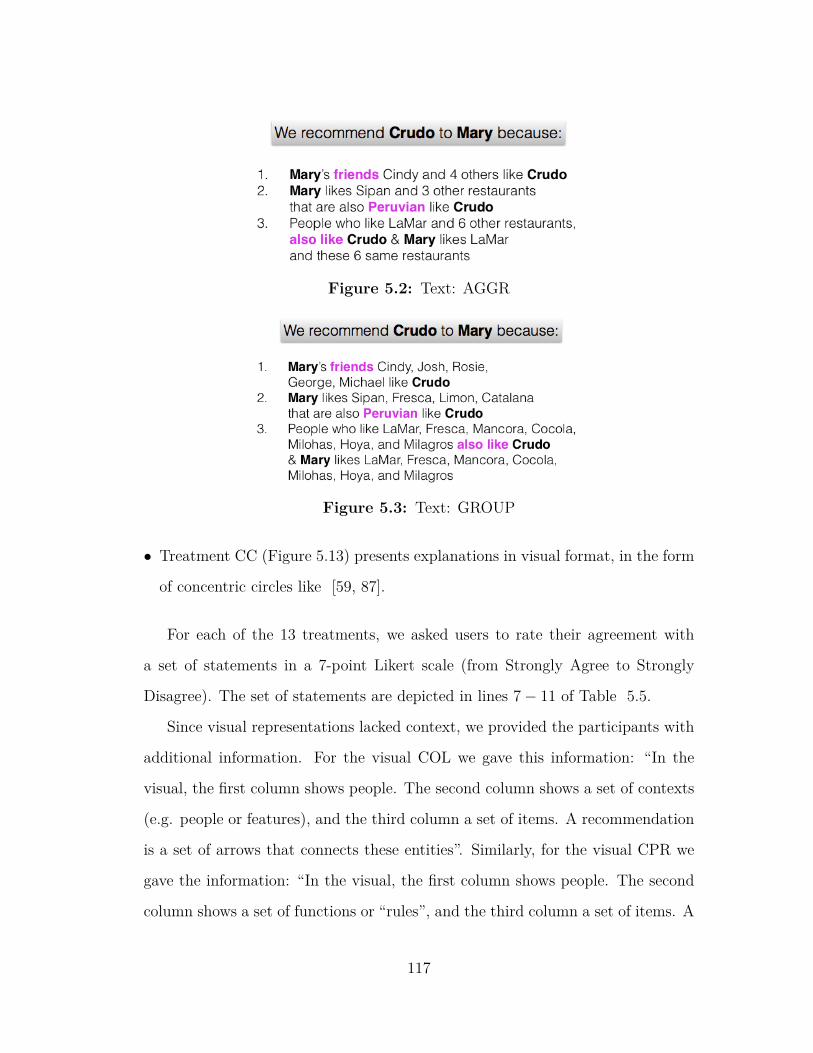
Figure 5.2: Text: AGGR

Figure 5.3: Text: GROUP

• Treatment CC (Figure 5.13) presents explanations in visual format, in the form

of concentric circles like [59, 87].

For each of the 13 treatments, we asked users to rate their agreement with

a set of statements in a 7-point Likert scale (from Strongly Agree to Strongly

Disagree). The set of statements are depicted in lines 7− 11 of Table 5.5.

Since visual representations lacked context, we provided the participants with

additional information. For the visual COL we gave this information: “In the

visual, the first column shows people. The second column shows a set of contexts

(e.g. people or features), and the third column a set of items. A recommendation

is a set of arrows that connects these entities”. Similarly, for the visual CPR we

gave the information: “In the visual, the first column shows people. The second

column shows a set of functions or “rules”, and the third column a set of items. A

117

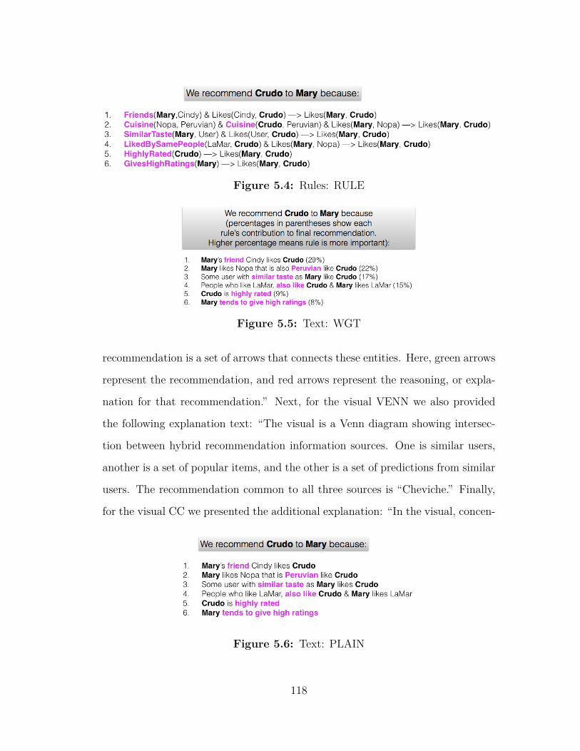
Figure 5.4: Rules: RULE

Figure 5.5: Text: WGT

recommendation is a set of arrows that connects these entities. Here, green arrows

represent the recommendation, and red arrows represent the reasoning, or expla-

nation for that recommendation.” Next, for the visual VENN we also provided

the following explanation text: “The visual is a Venn diagram showing intersec-

tion between hybrid recommendation information sources. One is similar users,

another is a set of popular items, and the other is a set of predictions from similar

users. The recommendation common to all three sources is “Cheviche.” Finally,

for the visual CC we presented the additional explanation: “In the visual, concen-

Figure 5.6: Text: PLAIN

118

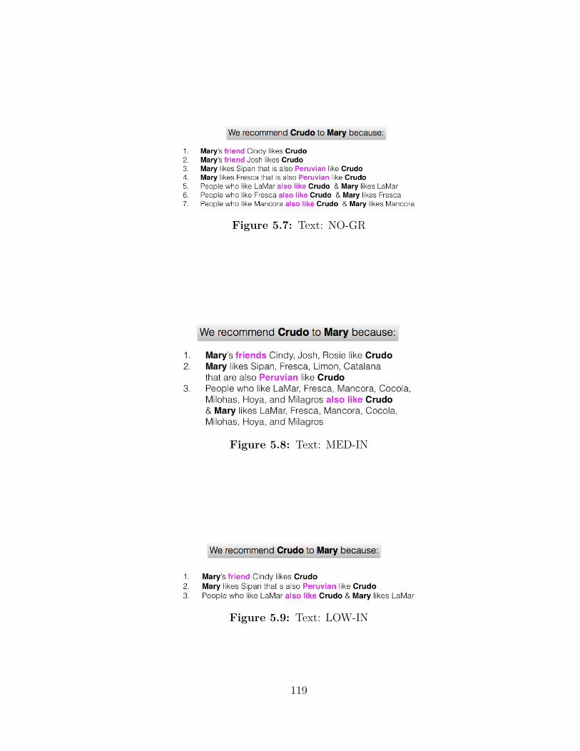
Figure 5.7: Text: NO-GR

Figure 5.8: Text: MED-IN

Figure 5.9: Text: LOW-IN

119

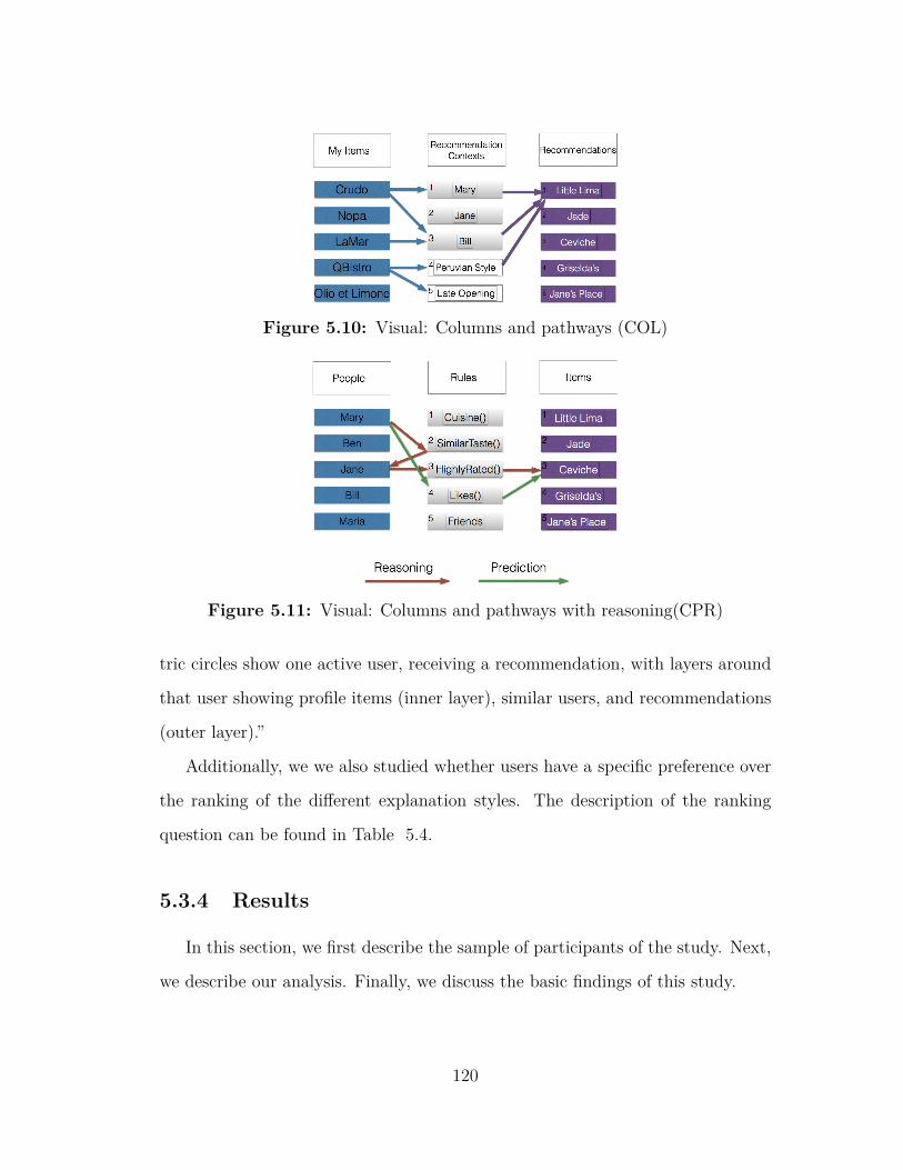
Figure 5.10: Visual: Columns and pathways (COL)

Figure 5.11: Visual: Columns and pathways with reasoning(CPR)

tric circles show one active user, receiving a recommendation, with layers around

that user showing profile items (inner layer), similar users, and recommendations

(outer layer).”

Additionally, we we also studied whether users have a specific preference over

the ranking of the different explanation styles. The description of the ranking

question can be found in Table 5.4.

5.3.4 Results

In this section, we first describe the sample of participants of the study. Next,

we describe our analysis. Finally, we discuss the basic findings of this study.

120

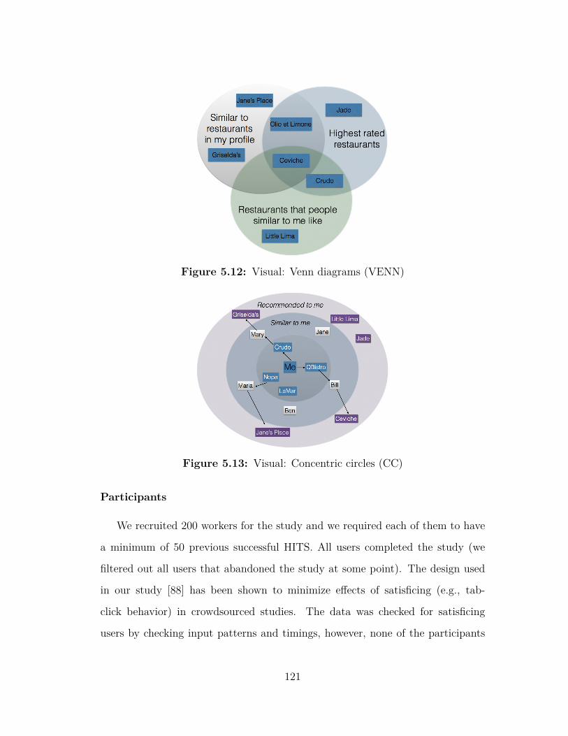
Figure 5.12: Visual: Venn diagrams (VENN)

Figure 5.13: Visual: Concentric circles (CC)

Participants

We recruited 200 workers for the study and we required each of them to have

a minimum of 50 previous successful HITS. All users completed the study (we

filtered out all users that abandoned the study at some point). The design used

in our study [88] has been shown to minimize effects of satisficing (e.g., tab-

click behavior) in crowdsourced studies. The data was checked for satisficing

users by checking input patterns and timings, however, none of the participants

121

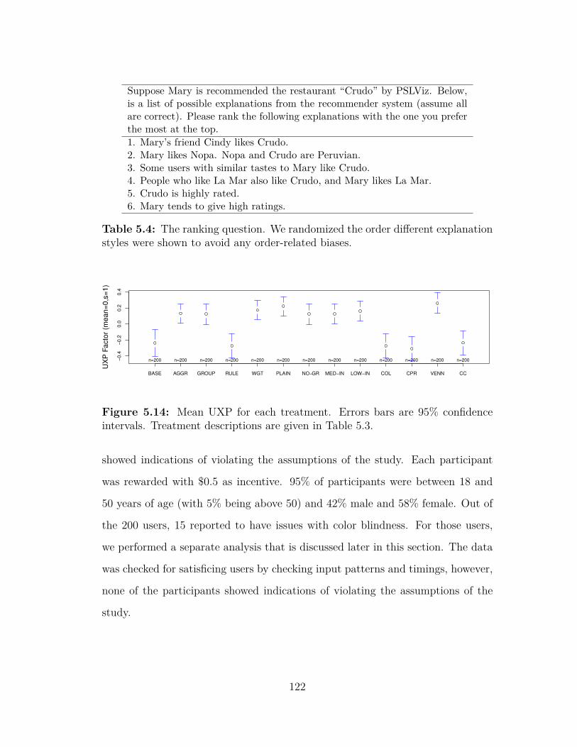
Suppose Mary is recommended the restaurant “Crudo” by PSLViz. Below,is a list of possible explanations from the recommender system (assume allare correct). Please rank the following explanations with the one you preferthe most at the top.1. Mary’s friend Cindy likes Crudo.2. Mary likes Nopa. Nopa and Crudo are Peruvian.3. Some users with similar tastes to Mary like Crudo.4. People who like La Mar also like Crudo, and Mary likes La Mar.5. Crudo is highly rated.6. Mary tends to give high ratings.

Table 5.4: The ranking question. We randomized the order different explanationstyles were shown to avoid any order-related biases.

−0.4

−0.2

0.0

0.2

0.4

UX

P F

acto

r (m

ea

n=

0,s

=1

)

BASE AGGR GROUP RULE WGT PLAIN NO−GR MED−IN LOW−IN COL CPR VENN CC

n=200 n=200 n=200 n=200 n=200 n=200 n=200 n=200 n=200 n=200 n=200 n=200 n=200

Figure 5.14: Mean UXP for each treatment. Errors bars are 95% confidenceintervals. Treatment descriptions are given in Table 5.3.

showed indications of violating the assumptions of the study. Each participant

was rewarded with $0.5 as incentive. 95% of participants were between 18 and

50 years of age (with 5% being above 50) and 42% male and 58% female. Out of

the 200 users, 15 reported to have issues with color blindness. For those users,

we performed a separate analysis that is discussed later in this section. The data

was checked for satisficing users by checking input patterns and timings, however,

none of the participants showed indications of violating the assumptions of the

study.

122

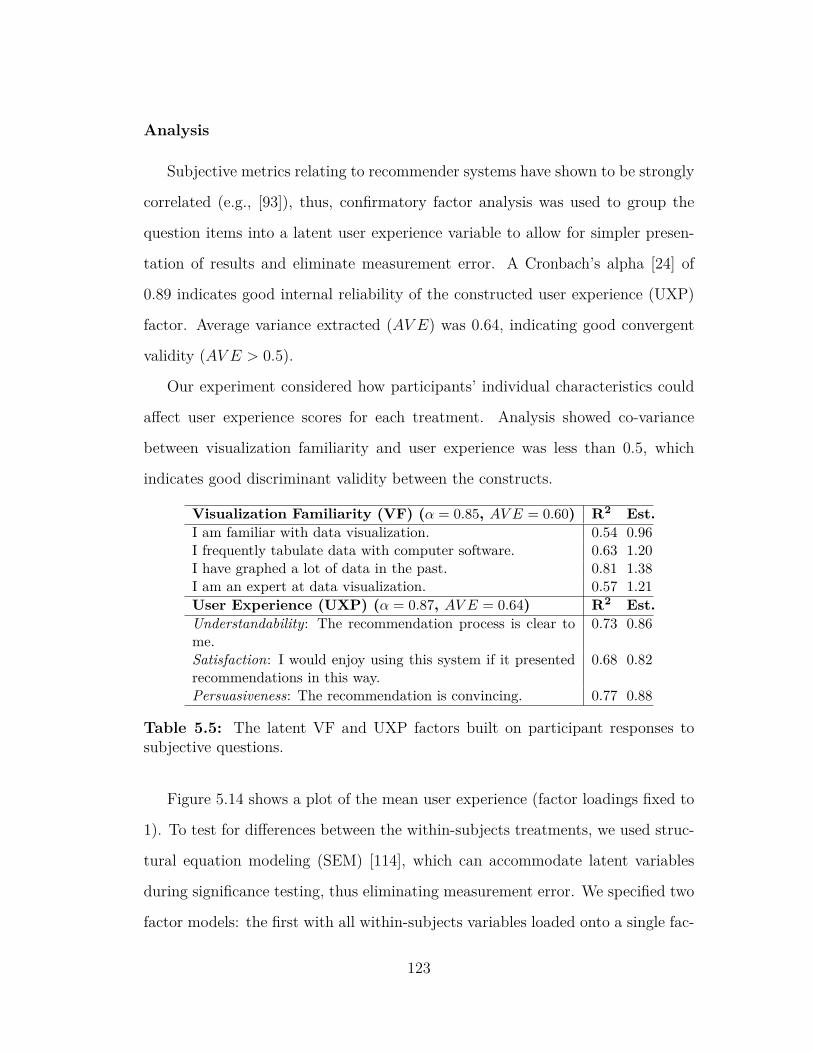
Analysis

Subjective metrics relating to recommender systems have shown to be strongly

correlated (e.g., [93]), thus, confirmatory factor analysis was used to group the

question items into a latent user experience variable to allow for simpler presen-

tation of results and eliminate measurement error. A Cronbach’s alpha [24] of

0.89 indicates good internal reliability of the constructed user experience (UXP)

factor. Average variance extracted (AV E) was 0.64, indicating good convergent

validity (AV E > 0.5).

Our experiment considered how participants’ individual characteristics could

affect user experience scores for each treatment. Analysis showed co-variance

between visualization familiarity and user experience was less than 0.5, which

indicates good discriminant validity between the constructs.

Visualization Familiarity (VF) (α = 0.85, AV E = 0.60) R2 Est.I am familiar with data visualization. 0.54 0.96I frequently tabulate data with computer software. 0.63 1.20I have graphed a lot of data in the past. 0.81 1.38I am an expert at data visualization. 0.57 1.21User Experience (UXP) (α = 0.87, AV E = 0.64) R2 Est.Understandability: The recommendation process is clear tome.

0.73 0.86

Satisfaction: I would enjoy using this system if it presentedrecommendations in this way.

0.68 0.82

Persuasiveness: The recommendation is convincing. 0.77 0.88

Table 5.5: The latent VF and UXP factors built on participant responses tosubjective questions.

Figure 5.14 shows a plot of the mean user experience (factor loadings fixed to

1). To test for differences between the within-subjects treatments, we used struc-

tural equation modeling (SEM) [114], which can accommodate latent variables

during significance testing, thus eliminating measurement error. We specified two

factor models: the first with all within-subjects variables loaded onto a single fac-

123

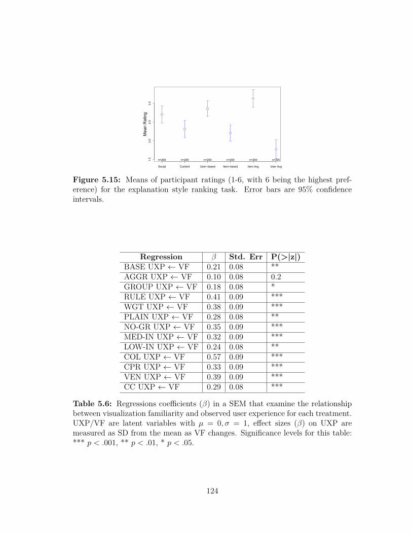
1.5

2.0

2.5

3.0

Mea

n R

atin

g

Social Content User−based Item−based Item Avg User Avg

n=200 n=200 n=200 n=200 n=200 n=200

Figure 5.15: Means of participant ratings (1-6, with 6 being the highest pref-erence) for the explanation style ranking task. Error bars are 95% confidenceintervals.

Regression β Std. Err P(>|z|)BASE UXP ← VF 0.21 0.08 **AGGR UXP ← VF 0.10 0.08 0.2GROUP UXP ← VF 0.18 0.08 *RULE UXP ← VF 0.41 0.09 ***WGT UXP ← VF 0.38 0.09 ***PLAIN UXP ← VF 0.28 0.08 **NO-GR UXP ← VF 0.35 0.09 ***MED-IN UXP ← VF 0.32 0.09 ***LOW-IN UXP ← VF 0.24 0.08 **COL UXP ← VF 0.57 0.09 ***CPR UXP ← VF 0.33 0.09 ***VEN UXP ← VF 0.39 0.09 ***CC UXP ← VF 0.29 0.08 ***

Table 5.6: Regressions coefficients (β) in a SEM that examine the relationshipbetween visualization familiarity and observed user experience for each treatment.UXP/VF are latent variables with µ = 0, σ = 1, effect sizes (β) on UXP aremeasured as SD from the mean as VF changes. Significance levels for this table:*** p < .001, ** p < .01, * p < .05.

124

tor (null hypothesis: no differences between treatments); the second with a factor

specified for each of the 13 treatments (hypothesis: treatments cause a change in

UXP). The model with a factor specified for each treatment achieved better fit.

We used the Akaike Information Criterion (AIC) to estimate the quality of each

model (a lower AIC indicates better comparative fit) and achieved AIC = 25838

for the single factor model vs. AIC = 22908 for the model with a factor for

each treatment. This result indicates that there exist differences in UXP between

treatments and thus the null hypothesis is rejected.

Next, we performed post-hoc tests between each treatment using a Raykov

change model [97] (this mimics the popular Tukey test [113] while still allowing

the use of latent variables). In this method, one factor (treatment) is used as a

baseline and a slope is calculated between it and another factor. The post-hoc

test showed that the interface using Venn diagrams (VENN) was significantly

better than all other visual treatments and the baseline (p < 0.001 for BASE,

COL,CPR, and CC). VENN also performed significantly better than AGGR,

GROUP, NO-GR, MED-IN, and LOW-IN (∀ p < 0.05). The RULE treatment

performed significantly worse than the explanations in plain English, as well as

VENN (∀ p < 0.001). All English treatments performed significantly better than

the baseline BASE (∀ p < 0.001). There was no significant difference between any

of the English treatments (∀ p > 0.10), however, the mean for PLAIN was the

highest. Consequently, weights, information density, aggregation, and grouping

were also non-significant (∀ p > 0.10).

Results from the ranking task are shown in Figure 5.15. For our analysis

we converted the ranking into rating data, i.e., the item listed first was given a

rating of 6 and the item ranked last received rating 1. Users showed the strongest

preference for item average rating explanations, followed by user-based and social

125

explanations. A repeated measures ANOVA revealed differences in rating between

the explanation styles (p < 0.001). A Tukey post-hoc test showed no statistical

difference between social, user-based, and item average rating explanations (∀ p >

0.10). However, social, user-based, and item average rating were significantly

better than item-based and user average rating (∀ p < 0.05). User-based and item

average rating were significantly better than content explanations (both p < 0.05).

Finally, we conducted analysis on the relationship between visualization fa-

miliarity and user experience. A SEM was built with visualization familiarity

regressed onto user experience measurements for each treatment (Table 5.6). Re-

sults indicate that visualization familiarity predicts increased user experience in

all treatments, except AGGR. The highest increase in user experience is seen in

COL and RULE. Model fit: N = 200 with 174 free parameters, RMSEA =

0.064 (CI : [0.058, 0.069]), TLI = 0.89, CFI = 0.90 over null baseline model,

χ2(772) = 1397 (indicate acceptable fit, however, note that overall model fit is

not an indicator of whether effects exist between variables).

Answers to the Post-Study Questionnaire

At the end of the study, we asked users to give us any comments (in free text

format) regarding the study. The most interesting comments can be found in

Appendix 6.1.

5.3.5 Discussion

In this first user study, we presented an evaluation of different visualization

approaches using hybrid explanations. The results support prior findings [39] that

explanations improve the user experience of recommender systems.

More specifically, Venn diagrams outperform all other visual interfaces and

126

five of seven English interfaces, but are difficult to adapt to more than three

sources. Natural language approaches were preferable to rule groundings from

HyPER. Our experiments did not show a statistically significant difference across

dimensions such as weights, information density, aggregation, or grouping in these

explanations. This suggests that most plain English explanations may perform

more or less the same in recommendation settings. Our results indicated that

social, user-based, and item average rating explanations were the preferred ex-

planation styles by users. Furthermore, we have established a reliable scale, as

evidenced by Cronbach’s α, for visualization familiarity which might be used to

tailor explanation styles to individual users.

Additionally, we discovered that color-blind users (N = 14) rated the RULE

interface higher in terms of UXP than the rest of the sampled population, with

marginal significance (β = 0.15, p = 0.051). The mockup for this interface used

a fairly intense violet color which may have been difficult to read for all but the

colorblind users. While the colorblind sample was not large enough to change the

results of the study, it highlights the need to accommodate these types of users

when evaluating UXP for recommender systems.

The mockups that we showed to users were manually produced and not gen-

erated by the HyPER system. As a result, the study was synthetic and did not

support personalization. To analyze factors such as the quality of the recommen-

dation and whether users agree and connect with the evidence, we conducted a

personalized user study that we present in the next section.

127

5.4 Second Study: Personalized Hybrid Expla-

nations

In this Section we describe the second personalized user study on hybrid ex-

planations. More specifically, in Section 5.4.1 we describe the properties of the

last.fm dataset. In Section 5.4.2 we define the research questions we aim to answer

with this study. In Section 5.4.3 we give an overview of the user study and in

Section 5.4.4 we present the results which answer the research questions. Finally,

in Section 5.4.5 we summarize our findings.

5.4.1 Last.fm Dataset

In this Chapter, we use the domain of music to demonstrate our hybrid rec-

ommendation model and explanations. We use data from the last.fm website for

two reasons: i) last.fm provides an API1 offering convenient access to music data

and ii) last.fm contains a wide range of information that can be exploited by our

hybrid model: friendships among users, rating history for users, content informa-

tion for artists (in the form of tags), and popular artists in the database. The

Last.fm exposes two main API types, Users and Artists. The User API provides

access to user demographic information (e.g. country of origin), user’s top artists

by listening frequency, and user’s friends. The Artist API provides access to sim-

ilar artists to a given artist based on both CF and tag information and the top

user-provided tags for an artist. Last.fm also offers general top-chart methods

returning information such as the k artists with the highest number of listeners

or playcounts as well as the k tags appearing the highest number of times across

last.fm’s database. In order to integrate with last.fm’s API we built a crawler1https://www.last.fm/api

128

using pylast2 that allows us to collect information for each user in our study in

real time.

5.4.2 Research Questions

We structure our work around answering the following four fundamental ques-

tions about recommendations and explanations coming from a hybrid system:

1. What is HyPER-music’s performance for online recommendations?

The HyPER framework [65] has reported state-of-the-art performance for

the rating task in an offline setting for two different datasets, i.e., business

and music recommendation. In this question, our goal is to measure the

accuracy of our modified version of the HyPER framework (HyPER-music)

in an online setting. To this end, we compare HyPER-music to a recom-

mender engine that recommends random artists from the last.fm dataset

(i.e., without taking into account any previous user preferences on artists).

2. How does explanation persuasiveness vary with different explana-

tion styles? An explanation from a hybrid recommender system usually

contains several different styles, such as user-based and social-based. In this

question, our goal is to study whether varying the different styles changes

the persuasiveness of an explanation. Additionally, following on from prior

work [110] showing that personality strongly correlates with user prefer-

ences, we study whether there is any difference in the preferred explanation

style when we take the users’ personality traits into account. Our hypoth-

esis is that users with specific personal characteristics will be persuaded by

different explanation styles. For example, an extrovert may be receptive2https://github.com/pylast/pylast

129

to social style explanations, while an introvert may prefer item-based style

explanations.

3. What is the ideal volume (i.e., number) of explanation styles? One

pitfall in explanatory systems is information overload. In this question,

we identify the inflection point in terms of volume, after which users lose

interest. We vary the volume of different explanation styles presented to a

user for each recommendation. Our hypothesis is that different volumes of

explanation styles will result in different persuasiveness levels. Our goal is to

determine the optimal number of explanation styles that balance information

overload and persuasiveness. We additionally study whether there is any

difference when we take the users’ personality traits into account, i.e., does

a user’s personality indicate their preference in terms of explanation volume?

4. How do explanation formats affect user experience? Prior work on

non-personalized explanations [69] showed that user experience is affected by

the format of the explanations, i.e., users prefer simple visual formats over

complex ones. Based on these results, in this work, we study the effect of

textual and simple visual formats (Venn diagrams and cluster dendrograms)

in personalized explanations. Our hypothesis is that different visual formats

will result in different levels of user experience.

5.4.3 Study Design

In this section, we describe our study from the point of view of one participant3. The study is divided in two phases. In the first phase, we ask the participant

to fill in a pre-questionnaire (this is the same for all participants). To improve ef-

ficiency in the study, while this step is in process, we crawl the music data for this3We use the AMT platform to recruit active last.fm participants.

130

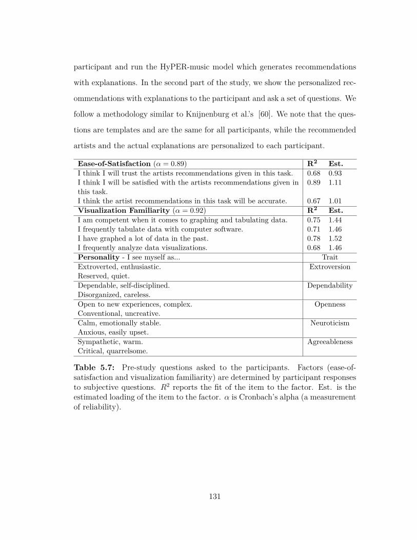
participant and run the HyPER-music model which generates recommendations

with explanations. In the second part of the study, we show the personalized rec-

ommendations with explanations to the participant and ask a set of questions. We

follow a methodology similar to Knijnenburg et al.’s [60]. We note that the ques-

tions are templates and are the same for all participants, while the recommended

artists and the actual explanations are personalized to each participant.

Ease-of-Satisfaction (α = 0.89) R2 Est.I think I will trust the artists recommendations given in this task. 0.68 0.93I think I will be satisfied with the artists recommendations given inthis task.

0.89 1.11

I think the artist recommendations in this task will be accurate. 0.67 1.01Visualization Familiarity (α = 0.92) R2 Est.I am competent when it comes to graphing and tabulating data. 0.75 1.44I frequently tabulate data with computer software. 0.71 1.46I have graphed a lot of data in the past. 0.78 1.52I frequently analyze data visualizations. 0.68 1.46Personality - I see myself as... TraitExtroverted, enthusiastic. ExtroversionReserved, quiet.Dependable, self-disciplined. DependabilityDisorganized, careless.Open to new experiences, complex. OpennessConventional, uncreative.Calm, emotionally stable. NeuroticismAnxious, easily upset.Sympathetic, warm. AgreeablenessCritical, quarrelsome.

Table 5.7: Pre-study questions asked to the participants. Factors (ease-of-satisfaction and visualization familiarity) are determined by participant responsesto subjective questions. R2 reports the fit of the item to the factor. Est. is theestimated loading of the item to the factor. α is Cronbach’s alpha (a measurementof reliability).

131

First Phase: Pre-study Questionnaire, Data Collection, and Generation

of Recommendations and Explanations

In this first phase of the study, we inform the participant that, in order to

participate, she needs to have a last.fm account with at least ten artists in her

profile and at least five friends. We prompt participants that are interested in

the study but do not have a last.fm account to follow detailed instructions on

how to create an account and enrich their profile with the prerequisites. After

the participant provides their last.fm id, we check that it meets the prerequisites.

If it does, we ask the participant to answer the pre-questionnaire, otherwise we

go back to informing the participant about the prerequisites and how to satisfy

them.

In the pre-study questionnaire we ask the participant questions related to the

ease-of-satisfaction in the field of music recommendations, as well as questions

related to visualization familiarity. We additionally ask questions related to the

five basic dimensions of personality, called the Big Five traits [110]. We adopt

the questionnaire by Gosling et al. [46] which has the advantage that it is very

brief and highly reliable. We report all the pre-study questions in the first column

of Table 5.7. Responses are provided using a 7-point Likert scale from “Totally

Disagree” to “Totally Agree”. During the time that the participant answers the

pre-study questions, in the background, we sequentially perform the following

tasks:

Crawl data: using the last.fm API methods described in Section 5.4.1, we crawl

the top 20 artists for this participant’s profile. Next, for each of these artists, we

crawl the top 20 tags and the top 20 most similar artists. For each similar artist,

we crawl the top 20 tags. Next, we retrieve the top 20 friends of this participant

along with their 20 most favorite artists.

132

Create candidate set: For the participant u of the study, we create a set of

candidate artists A = {a1, a2, . . . , an}. For each artist a ∈ A, we generate an

unobserved predicate Listens(u, a). Our HyPER-music model will make predic-

tions for all the unobserved Listens(u, a) predicates. Last.fm contains a large

number of artists, with the typical property that a large number of users listen

to a small number of artists (popular artists) and most of the artists have very

few users that listen to them (long tail). Since the generation of recommenda-

tions should be performed very quickly, we need to apply some selection criteria

in order to reduce the number of artists a ∈ A.4 At the same time, we want

the recommended artists to be personalized to each participant’s tastes. To this

end, for each participant we create a personalized set of candidate artists A which

consists of: (i) the 20 most similar artists (based on the last.fm similarity) in the

participant’s profile, (ii) the 20 top artists for each of this participant’s friends,

and (iii) the overall top 1000 artists in the last.fm database.

Compute similarities: we compute all the necessary similarities for the HyPER-

music model to run for this participant. More specifically, we compute: (i) simi-

larities between this participant and a subset of last.fm users (explained in detail

below) that generate data for grounding Rule 5.1 from Section 5.2, (ii) similarities

between the participant and his friends, generating data for Rule 5.6, and (iii)

similarities between the artists in the candidate set and the artists in the last.fm

database (both using CF and tag information). Similarities computed using CF

information generate data for Rule 5.2 and similarities using tag information gen-

erate data for Rule 5.4. The similarities that generate data for Rule 5.3 are already

computed by last.fm and we access them by calling the respective API method

for each artist. We should finally note that, when computing the CF user and

item similarities, the similarity computation is performed while the participant is4This process is usually performed in ranking tasks [1].

133

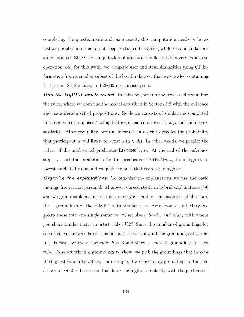
completing the questionnaire and, as a result, this computation needs to be as

fast as possible in order to not keep participants waiting while recommendations

are computed. Since the computation of user-user similarities is a very expensive

operation [84], for this study, we compute user and item similarities using CF in-

formation from a smaller subset of the last.fm dataset that we crawled containing

1475 users, 8672 artists, and 28639 user-artists pairs.

Run the HyPER-music model: In this step, we run the process of grounding

the rules, where we combine the model described in Section 5.2 with the evidence

and instantiate a set of propositions. Evidence consists of similarities computed

in the previous step, users’ rating history, social connections, tags, and popularity

statistics. After grounding, we run inference in order to predict the probability

that participant u will listen to artist a (a ∈ A). In other words, we predict the

values of the unobserved predicates Listens(u, a). At the end of the inference

step, we sort the predictions for the predicates Listens(u, a) from highest to

lowest predicted value and we pick the ones that scored the highest.

Organize the explanations: To organize the explanations we use the basic

findings from a non personalized crowd-sourced study in hybrid explanations [69]

and we group explanations of the same style together. For example, if there are

three groundings of the rule 5.1 with similar users Aren, Sonia, and Mary, we

group those into one single sentence: “User Aren, Sonia, and Mary with whom

you share similar tastes in artists, likes U2”. Since the number of groundings for

each rule can be very large, it is not possible to show all the groundings of a rule.

In this case, we use a threshold k = 3 and show at most 3 groundings of each

rule. To select which k groundings to show, we pick the groundings that involve

the highest similarity values. For example, if we have many groundings of the rule

5.1 we select the three users that have the highest similarity with the participant

134

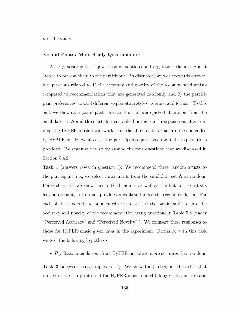
u of the study.

Second Phase: Main Study Questionnaire

After generating the top k recommendations and organizing them, the next

step is to present them to the participant. As discussed, we work towards answer-

ing questions related to 1) the accuracy and novelty of the recommended artists

compared to recommendations that are generated randomly and 2) the partici-

pant preferences’ toward different explanation styles, volume, and format. To this

end, we show each participant three artists that were picked at random from the

candidate set A and three artists that ranked in the top three positions after run-

ning the HyPER-music framework. For the three artists that are recommended

by HyPER-music, we also ask the participants questions about the explanations

provided. We organize the study around the four questions that we discussed in

Section 5.4.2:

Task 1 (answers research question 1): We recommend three random artists to

the participant, i.e., we select three artists from the candidate set A at random.

For each artist, we show their official picture as well as the link to the artist’s

last.fm account, but do not provide an explanation for the recommendation. For

each of the randomly recommended artists, we ask the participants to rate the

accuracy and novelty of the recommendation using questions in Table 5.8 (under

“Perceived Accuracy” and “Perceived Novelty” ). We compare these responses to

those for HyPER-music given later in the experiment. Formally, with this task

we test the following hypothesis:

• H1: Recommendations from HyPER-music are more accurate than random.

Task 2 (answers research question 2): We show the participant the artist that

ranked in the top position of the HyPER-music model (along with a picture and

135

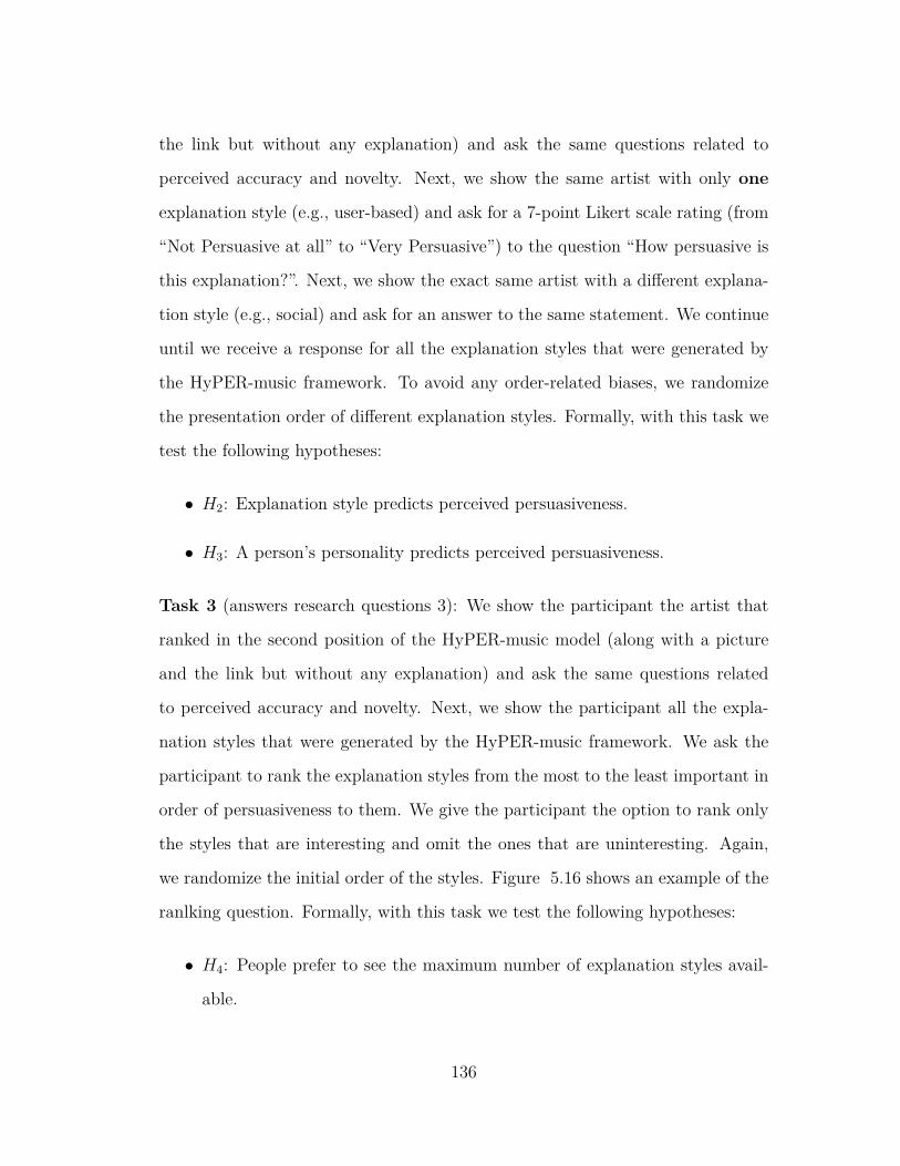
the link but without any explanation) and ask the same questions related to

perceived accuracy and novelty. Next, we show the same artist with only one

explanation style (e.g., user-based) and ask for a 7-point Likert scale rating (from

“Not Persuasive at all” to “Very Persuasive”) to the question “How persuasive is

this explanation?”. Next, we show the exact same artist with a different explana-

tion style (e.g., social) and ask for an answer to the same statement. We continue

until we receive a response for all the explanation styles that were generated by

the HyPER-music framework. To avoid any order-related biases, we randomize

the presentation order of different explanation styles. Formally, with this task we

test the following hypotheses:

• H2: Explanation style predicts perceived persuasiveness.

• H3: A person’s personality predicts perceived persuasiveness.

Task 3 (answers research questions 3): We show the participant the artist that

ranked in the second position of the HyPER-music model (along with a picture

and the link but without any explanation) and ask the same questions related

to perceived accuracy and novelty. Next, we show the participant all the expla-

nation styles that were generated by the HyPER-music framework. We ask the

participant to rank the explanation styles from the most to the least important in

order of persuasiveness to them. We give the participant the option to rank only

the styles that are interesting and omit the ones that are uninteresting. Again,

we randomize the initial order of the styles. Figure 5.16 shows an example of the

ranlking question. Formally, with this task we test the following hypotheses:

• H4: People prefer to see the maximum number of explanation styles avail-

able.

136

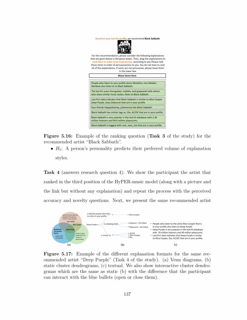
Basedonyourlast.fm profile,werecommendBlackSabbath.

Forthisrecommendation,pleaseconsiderthefollowingexplanationsthataregivenbelowinthegreenboxes.Then,dragtheexplanationstoranktheminorderofpersuasiveness,accordingtoyouPleaserank

theseitemsinorderofpersuasivenesstoyou.Youdonothavetorankalloftheexplanations,ifsomearenotpersuasive,pleaseleavethem

inthelowerbox.

Moveitemshere.

PeoplewholistentoyourprofileitemsMetallica,IronMaiden,Rainbow alsolistentotoBlackSabbath.

Thelast.fm usersGuruguhan,trojhlav,andgrapowski withwhomwhosharesimilarmusictastes,listentoBlackSabbath.

Last.fm’s dataindicatesthatBlackSabbathissimilartoAliceCooper,DeepPurple,Ozzy Osbourne thatareinyourprofile.

YourfriendsHappyDestroy,juliomencia likeBlackSabbath.

BlackSabbathhassimilartagsas:Dio,AC/DC thatareinyourprofile.

BlackSabbathisverypopularinthelast.fm databasewith2.36millionlistenersand94.6millionplaycounts.

BlackSabbathistaggedwithrock,seen_live thatareinyourprofile.

Figure 5.16: Example of the ranking question (Task 3 of the study) for therecommended artist “Black Sabbath”.• H5: A person’s personality predicts their preferred volume of explanation

styles.

Task 4 (answers research question 4): We show the participant the artist that

ranked in the third position of the HyPER-music model (along with a picture and

the link but without any explanation) and repeat the process with the perceived

accuracy and novelty questions. Next, we present the same recommended artist

DeepPurple

islikedbypeoplewholistentoartistsinyourprofile

isapopularartist

issimilarto

AliceCooper

Listeners=20million

Playcounts =49million

AC/DCAliceCooperDio

• PeoplewholistentotheartistAliceCooperthatisinyourprofilealsolistentoDeepPurple.

• DeepPurpleisverypopularinthelast.fm databasewith 20millionlistenersand49millionplaycounts.

• Last.fm’s dataindicatesthatDeepPurpleissimilartoAliceCooper,Dio,AC/DCthatareinyourprofile.

(a) (b) (c)

DeepPurple

AliceCooper

RadioHead,TheBeatles,Queen

Artiststhatarepopular

ArtistsinyourprofilethataresimilartoDeepPurple

Dio,AC/DC

Artiststhatarelikedbypeoplewholistentoartistsinyourprofile

Figure 5.17: Example of the different explanation formats for the same rec-ommended artist “Deep Purple” (Task 4 of the study). (a) Venn diagrams, (b)static cluster dendrograms, (c) textual. We also show intereactive cluster dendro-grmas which are the same as static (b) with the difference that the participantcan interact with the blue bullets (open or close them).

137

with the same explanation styles using different formats (one textual and three

visuals). For each format we ask the participant a 7-point Likert scale answer

to the set of user experience (UXP) statements presented in Table 5.8 (under

“Reception (UXP)”). To determine which visualizations to show, we use the results

of the crowd-sourced, but non-personalized, study [69]. According to that, Venn

diagrams significantly outperformed concentric circles and columns and pathways

(with or without reasoning) which participants found too complicated. Based on

this finding, we show the participants Venn diagrams and two very simple forms

of pathways among columns, i.e., two cluster dendrograms, one static and one

interactive. Figure 5.17 illustrates an example of the different formats shown to

the same participant for the recommended artist “Deep Purple”. For the cluster

dendrograms we show only the static version. The difference between the two

versions of the cluster dendrograms is that in the first case, we present all the

visualization information at once and there is no option for interaction, while

in the second case we hide some of the information and ask the participants to

interact with the blue bullets (open or close them) of the diagram in order to reveal

all the information available. We note that since Venn diagrams can accommodate

three different styles, we restrict all the other visual and textual explanations to

show only three styles. To select which three out of the seven offered styles to

show, we choose the three styles reported to improve performance in prior work,

i.e., user-based, item-based CF, and popularity-based. As before, we randomize

the order that we show the different formats. Formally, with this task we test the

following hypothesis:

• H6: Explanation format predicts a person’s reception (UXP) of an explana-

tion.

Finally, in the middle of the study we ask the satisficing question: “Please

138

answer “Somewhat not Persuasive” to this question”. This question, which is the

same for all participants, helps us to test for satisficing.

Perceived Accuracy (α = 0.96) R2 Est.The recommended artist represents my tastes. 0.86 1.05This is an accurate recommendation 0.88 1.05I like the recommended artist. 0.93 1.06Perceived Novelty (α = 0.94) R2 Est.I have never listened to this artist before. 0.91 1.44I am aware of the recommended artist. 0.74 1.19The recommended artist is new to me. 0.91 1.45Reception (UXP) (α = 0.93) R2 Est.(Confidence): This explanation makes me confident that I will like thisartist.

0.73 1.04

(Transparency): This explanation makes the recommendation processclear to me.

0.71 1.06

(Satisfaction): I would enjoy using a recommendation system if it pre-sented recommendations in this way.

0.79 1.17

(Persuasiveness): This explanation for the recommendation is convinc-ing.

0.88 1.19

Table 5.8: Questions for the main study asked to the participants. Again, factors(perceived accuracy, perceived novelty, and UXP) are determined by participantresponses to subjective questions. As before, we report R2, Est., and Cronbach’salpha.

5.4.4 Results

In this section, we first describe the sample of participants of the study. Next,

we report the factors created from the subjective questions along with statistics

related to the fit. Next, we report the results of the study and hypotheses testing.

Significance levels in this section are reported as follows: *** = p < .001, ** =

p < .01, and * = p < .05. Finally, we discuss the basic findings of this study.

139

Participants

We collected 212 samples of within-subjects participant data using Amazon’s

Mechanical Turk. Overall, 92% of participants were between 18 and 50 years of

age, and 60% were male. Each participant was rewarded with $3 as incentive.

Satisficing, the practice of gaming research studies, is a legitimate concern for any

crowd-sourced platform [56]. We checked the data for satisficing participants by

carefully examining input/timing patterns and checking the answer to the satis-

ficing question. After filtering out participants that exhibited satisficing behavior,

there were N = 198 samples for analysis.

Factor Fit

In Tables 5.7 and 5.8 we report with bold the factors that were confirmed from

participant responses on the subjective questions. Next to each factor, we show

a measurement of internal reliability (Cronbach’s α [108]) for each dependent

variable that was solicited via the questionnaires. All factors achieved good or

excellent internal reliability. All factors achieved good discriminant validity using

the Campbell & Fiske test [15]. To improve modeling of personality traits (which

were not factored), we load a different latent variable on each response with a

fixed value (1). Then, we free the variance of each response and fix the variance

of the latent variable to the variance of the response.

Effectiveness of Hybrid Recommendations

As discussed, to validate the quality of the recommendations generated by the

HyPER-music framework, for each recommended artist (throughout the study) we

asked the participants questions related to perceived accuracy and novelty of the

recommendation. We compared the predictions from HyPER-music with random

140

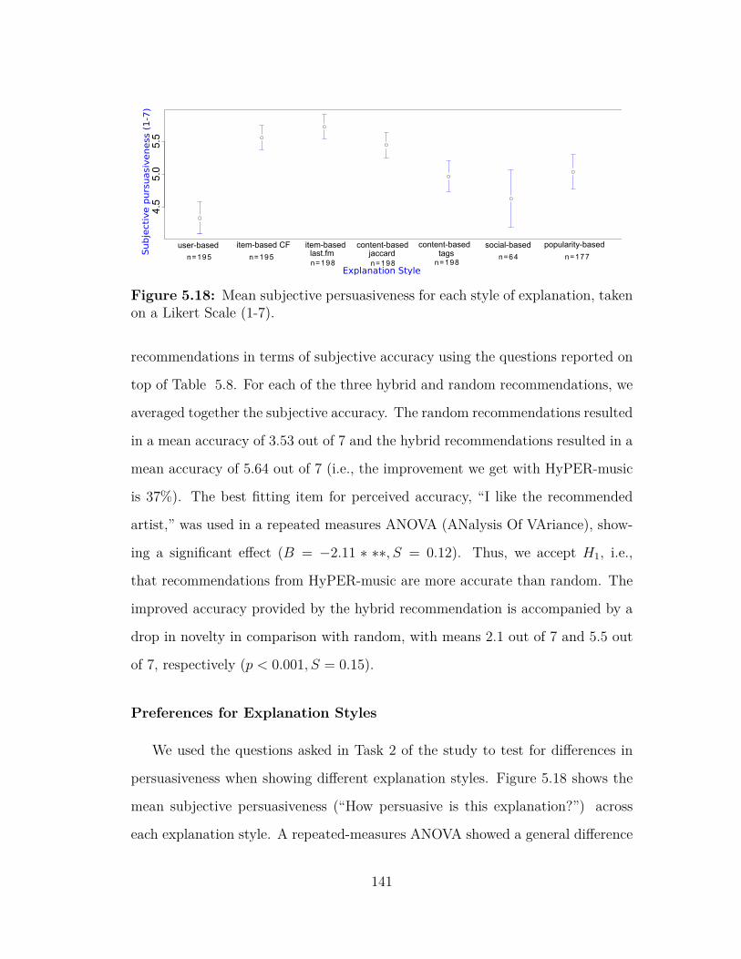
4.5

5.0

5.5

Explanation Style

Subje

cti

ve p

urs

uasi

veness

(1

-7)

item-basedlast.fm

content-basedjaccard

content-basedtags

social-based popularity-based

n=195 n=195n=198 n= 198 n=198

n=64 n=177

user-based item-based CF

Figure 5.18: Mean subjective persuasiveness for each style of explanation, takenon a Likert Scale (1-7).

recommendations in terms of subjective accuracy using the questions reported on

top of Table 5.8. For each of the three hybrid and random recommendations, we

averaged together the subjective accuracy. The random recommendations resulted

in a mean accuracy of 3.53 out of 7 and the hybrid recommendations resulted in a

mean accuracy of 5.64 out of 7 (i.e., the improvement we get with HyPER-music

is 37%). The best fitting item for perceived accuracy, “I like the recommended

artist,” was used in a repeated measures ANOVA (ANalysis Of VAriance), show-

ing a significant effect (B = −2.11 ∗ ∗∗, S = 0.12). Thus, we accept H1, i.e.,

that recommendations from HyPER-music are more accurate than random. The

improved accuracy provided by the hybrid recommendation is accompanied by a

drop in novelty in comparison with random, with means 2.1 out of 7 and 5.5 out

of 7, respectively (p < 0.001, S = 0.15).

Preferences for Explanation Styles

We used the questions asked in Task 2 of the study to test for differences in

persuasiveness when showing different explanation styles. Figure 5.18 shows the

mean subjective persuasiveness (“How persuasive is this explanation?”) across

each explanation style. A repeated-measures ANOVA showed a general difference

141

between explanation styles (F = 32.635, p < 0.0001). Thus, we accept H2, i.e.,

explanation style predicts perceived persuasiveness. A Tukey post-hoc test [113]

showed significant improvements by item-based CF, content-based Jaccard, and

item-based Last.fm styles over user-based (∀p < 0.001), popularity-based (∀p <

0.025), content-based tags (∀p < 0.001), and social-based (∀p < 0.001). No

significant improvement was found for item-based Last.fm over item-based CF, or

content-based Jaccard.

To test the significance of personality traits in the persuasiveness of an expla-

nation, we conducted an exploratory structural equation modeling (SEM) [114]

analysis. It is well known that people may change their ratings of items based on

user experience or persuasive explanations [52], so we accounted for this effect by

controlling for the accuracy/novelty of each recommendation and the participant’s

self-reported ease of satisfaction. Then, we tested for an effect of each of the ten

personality traits on the seven different explanation styles by performing a regres-

sion between each. This resulted in a total of 70 hypotheses, so we controlled for

multiplicity via the Benjamini-Hochberg procedure with Q = 0.10 [7], which is

recommended for exploratory SEM analysis [23].

Figure 5.19 shows the results from the exploratory analysis. Of the ten person-

ality traits, only four were shown to have a significant bearing on persuasiveness of

the explanation (dependable, calm, anxious, critical). These four responses could

be grouped into their larger personality traits: conscientiousness (dependable),

neuroticism (anxious, calm), and agreeableness (critical). Conscientious partici-

pants reported being easier to satisfy. The participants seemed to be split in terms

of neuroticism: calm participants tended to be more receptive of popularity-based

explanations while anxious tended to be more receptive of item-based CF expla-

nations. If the participant identified as dependable and calm or anxious and criti-

142

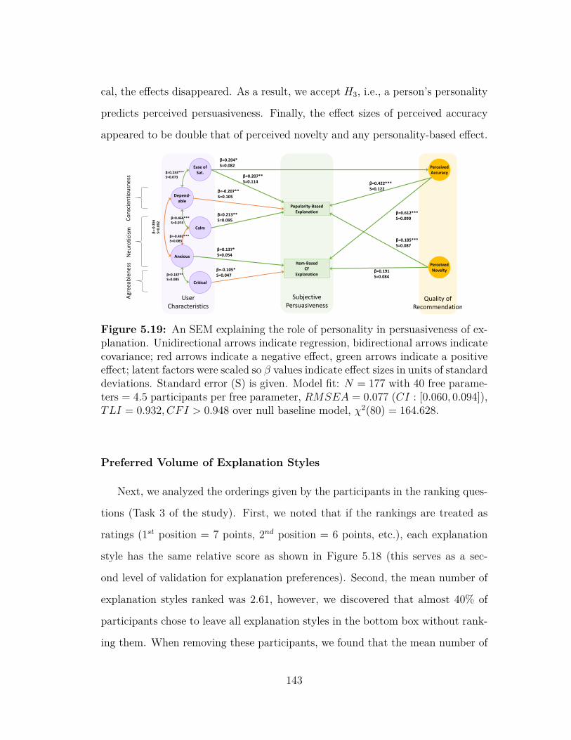
cal, the effects disappeared. As a result, we accept H3, i.e., a person’s personality

predicts perceived persuasiveness. Finally, the effect sizes of perceived accuracy

appeared to be double that of perceived novelty and any personality-based effect.

Quality ofRecommendation

SubjectivePersuasiveness

UserCharacteristics

Ease ofSat.

PerceivedAccuracy

Item-BasedCF

Explanation

PerceivedNovelty

β=0.2049S=0.082

Popularity-BasedExplanation

Critical

Anxious

Depend-able

Calm

β=-0.1059S=0.047

β=0.1379S=0.054

β=-0.20799S=0.105

β=0.21399S=0.095

β=0.612999S=0.090

β=0.422999S=0.122

β=0.20799S=0.114

β=0.185999S=0.087

β=0.191S=0.084

Conscientiousness

Neu

roticism

β=0.233999S=0.073

β=-0.356

S=0.092

β=0.464999S=0.074

β=-0.492999S=0.085

β=0.18799S=0.085

Agreeableness

Figure 5.19: An SEM explaining the role of personality in persuasiveness of ex-planation. Unidirectional arrows indicate regression, bidirectional arrows indicatecovariance; red arrows indicate a negative effect, green arrows indicate a positiveeffect; latent factors were scaled so β values indicate effect sizes in units of standarddeviations. Standard error (S) is given. Model fit: N = 177 with 40 free parame-ters = 4.5 participants per free parameter, RMSEA = 0.077 (CI : [0.060, 0.094]),TLI = 0.932, CFI > 0.948 over null baseline model, χ2(80) = 164.628.

Preferred Volume of Explanation Styles

Next, we analyzed the orderings given by the participants in the ranking ques-

tions (Task 3 of the study). First, we noted that if the rankings are treated as

ratings (1st position = 7 points, 2nd position = 6 points, etc.), each explanation

style has the same relative score as shown in Figure 5.18 (this serves as a sec-

ond level of validation for explanation preferences). Second, the mean number of

explanation styles ranked was 2.61, however, we discovered that almost 40% of

participants chose to leave all explanation styles in the bottom box without rank-

ing them. When removing these participants, we found that the mean number of

143

explanation styles was 4.32. To test H4 (people prefer to see the maximum num-

ber of explanation styles available), we conducted a one-sample t-test to check if

the mean of the sample was significantly different than 7, which was the max-

imum volume of available explanation styles. We found a significant difference

(t = −22.9, p < 0.001), which remained significant when omitting participants

who had not ranked any explanations (t = −13.8, p < 0.001). Thus we reject H4,

concluding that people lose interest after approximately three to four explana-

tion styles. Finally, we tested whether or not personality predicted the volume of

explanation styles ranked. We tested ten regressions (multiplicity control again

with Q = 0.10) within an SEM which revealed that dependable people were likely

to rank less (β = −0.166∗, S = 0.15) and open people were likely to rank more

(β = 0.212∗∗, S = 0.144). Thus we accept H5, i.e., a person’s personality predicts

their preferred volume of explanation styles.

Textual vs. Visual Formats

As discussed, in Task 4 of the study, for one artist we showed four different

explanation formats (one textual and three visual) and asked participants to an-

swer a set of UXP questions reported in Table 5.8. We plot the persuasiveness

score, which reported the best R2 value, for each visual/textual format in Fig-

ure 5.20. A repeated-measures ANOVA showed a difference between treatments

(F = 10.13, p < 0.001). Therefore, we accept H6, i.e., explanation format predicts

a user’s reception of an explanation. Specifically, text explanations were perceived

as more persuasive than every visual format (∀p < 0.001). To investigate further,

we considered whether visualization familiarity predicted better reception of the

visual formats. Four regressions were tested in an SEM when controlling for the

accuracy of the recommendation and self-reported ease-of-satisfaction, showing

144

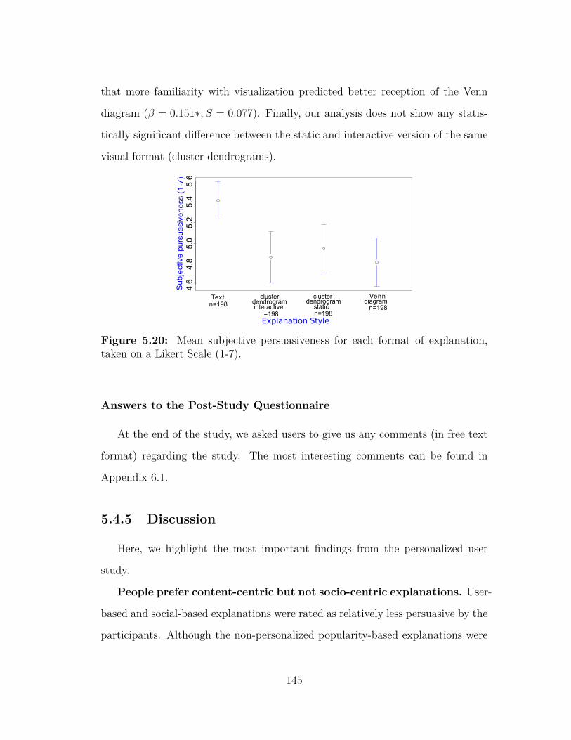
that more familiarity with visualization predicted better reception of the Venn

diagram (β = 0.151∗, S = 0.077). Finally, our analysis does not show any statis-

tically significant difference between the static and interactive version of the same

visual format (cluster dendrograms).

4.6

4.8

5.0

5.2

5.4

5.6

Text clusterdendrogram

Vennclusterdendrogram

interactive staticn=198

n=198 n=198n=198

diagram

Explanation Style

Su

bje

ctiv

e p

urs

ua

sive

ne

ss (

1-7

)

Figure 5.20: Mean subjective persuasiveness for each format of explanation,taken on a Likert Scale (1-7).

Answers to the Post-Study Questionnaire

At the end of the study, we asked users to give us any comments (in free text

format) regarding the study. The most interesting comments can be found in

Appendix 6.1.

5.4.5 Discussion

Here, we highlight the most important findings from the personalized user

study.

People prefer content-centric but not socio-centric explanations. User-

based and social-based explanations were rated as relatively less persuasive by the

participants. Although the non-personalized popularity-based explanations were

145

rated more favorably, they were still significantly less persuasive than the content-

based explanations. Moreover, we discovered that calm participants (low neuroti-

cism) preferred popularity-based explanations, while anxious participants (high

neuroticism) preferred item-based CF explanations. Calm participants were also

likely to be sympathetic and extroverted which may explain their higher recep-

tiveness to popular items. Additionally, participants that identified as dependable

did not have any preference for the popularity-based explanation, potentially sug-

gesting they are less sensitive by popular opinion. Likewise, neurotic participants

(who were also likely to be introverted and reserved), showed a slight preference

for item-based CF explanations, which surface patterns of particular tastes shared

with others.

People prefer to see at most three to four explanations. Our analysis

of the varying volume of explanation styles indicates that a relatively large per-

centage of users prefer to see no explanation with a recommendation, a possible

artifact of our experimental design. For the rest of the participants, we find that

the average number of explanations they prefer is 4.32. We also discovered that

open participants were persuaded by many explanations, while conscientious par-

ticipants preferred fewer. We believe this due to the fact that open participants

seek new experiences, while conscientious participants are turned off by clutter

and disorganization. However, despite the significant effects, due to the corre-

lation between those two traits and relatively low effect sizes, personalization of

explanation volume may be unnecessary. A default of three to four explanations

would be sufficient for most people. We recommend follow-up work specifically to

target the role of neuroticism in explanation reception.

Textual explanations are ideal. Our analysis indicates that text explana-

tions were perceived as more persuasive compared to three different visual formats.

146

When considering visualization familiarity as a control variable, we find that users

with more familiarity in visualization are more receptive to the Venn diagrams.

Despite this, our model did not predict that participants familiar with visualiza-

tion would prefer the Venn diagram over the text explanations. As a result, we

believe that textual explanations would likely satisfy nearly everyone. Finally, our

analysis does not show any statistically significant difference between the static

and interactive versions of the same visual format (cluster dendrograms).

5.5 Conclusion and Future Work

In this work, we proposed the HyPER-music recommender system which ex-

tends the HyPER model and generates music recommendations with a variety

of explanation styles in real time. We conducted two user studies: i) a non-

personalized study where we evaluated different visualization approaches using

hybrid explanations, and ii) a personalized study where users evaluated the ac-

curacy of recommendations and persuasiveness of different explanations under

varying the styles, volume, and format.

In our future work, we plan to support a conversational recommender sys-

tem that will use the observations from interactions with users and adjust the

explanations based on their preferences. Additionally, we are interested in ex-

tending the HyPER framework to take into account the explanations during the

process of generating the predictions. We want to study whether incorporating

the explanations in the prediction process has any effect on the accuracy of the

recommendations. Finally, we plan to focus on explanation design in scenarios

where users have limited space or time for exploring the explanations.

147

Chapter 6

Conclusion

In this dissertation, I presented a collective probabilistic approach that is gen-

eralizable, scalable and can offer on-demand, accurate recommendations and ex-

planations over richly-structured social networks. I organized my work around

three core areas that are fundamendal for recommendations over richly-structured

networks: 1) entity resolution that aims at aggregating different views of a het-

erogenous network, 2) a hybrid recommender that exploits the rich structure of

social networks and can incorporate information coming from a variety of informa-

tion sources, and 3) explanations of the complex reasoning behind the proposed

recommendations to users.

In my work, I formulated the problems of entity resolution, recommendation,

and explanation as inference in a graphical model. To create my models and

reason over the graphs, I built upon a statistical relational learning framework

called probabilistic soft logic. My models, which allow for scalable, collective in-

ference, showed an improved performance over state-of-the-art methods by lever-

aging richly-structured data, i.e., relational features (such as user similarities),

complex relationships (such as mutual exclusion), a variety of similarity mea-

sures, as well as other heterogenous data sources (such as predictions from other

148

algorithms).

In the area of entity resolution, I implemented a collective classification ap-

proach based on PSL. My contributions include (1) a scalable entity resolution

framework that effectively combines attributes, relational information, logical con-

straints, and predictions from other algorithms, (2) a method for learning how to

balance the different similarity scores and relational features, (3) extensive ex-

perimental studies on two real-world datasets where it is demonstrated that the

framework can effectively combine different signals, resulting in improved per-

formance over state-of-the-art approaches on two datasets, and (4) a set of con-

clusions from the experimental evaluation that can be used by entity resolution

practitioners. More specifically, the experimental studies showed that: i) name

similarities are not enough for the task of entity resolution in relational domains,

ii) the addition of attribute information results in a notable increase in the perfor-

mance, iii) first-degree relationships help most in low noise scenarios, iv) collective

relations yield substantial improvements, v) incorporating predictions from other

algorithms always improves performance, vi) the performance of different entity

resolution models changes when the string similarity functions change, while the

setting of string similarity functions that performs best is different for each model.

In the area of hybrid recommendations, I implemented a hybrid recommender

system called HyPER. My contributions include (1) a general and extensible hy-

brid recommender system with PSL, (2) a method for learning how to balance the

different input signals in the hybrid system, and (3) extensive experimental studies

on several information sources which validate the performance of the framework

and highlight the contribution of each source to the final prediction. The HyPER

framework is the first to provide a mechanism for incorporating and reasoning over

additional information sources as they become available. Experimental evaluation

149

of the approach on two popular recommendation datasets, showed that HyPER

effectively combined multiple information types for improved performance and

significantly outperformed existing state-of-the-art approaches.

In the area of explanations, I extend HyPER to provide hybrid personalized

explanations. My contributions include (1) a method for generating hybrid ex-

planations from a hybrid recommender system built in PSL, (2) a list of ways

explanations can be presented such as varying the textual and visual formats,

the explanation styles, as well as the volume of the explanations, and (3) two

large crowd-sourced user studies (a personalized and a non-personalized) which

generated a set of conclusions useful for designers of hybrid explanation inter-

faces. In particular, the key conclusions of the non-personalized study were that

Venn diagrams outperformed all other visual interfaces, while natural language

approaches were preferable to rule groundings from HyPER. The key conclusions

of the second personalized study were the following: i) people prefer to see at

most three to four explanations, ii) textual explanations are ideal, and iii) people

prefer item-centric over user-centric explanations.

From a modeling perspective, all three areas of entity resolution, recommen-

dation, and explanation present commonalities that I have leveraged in order to

deliver improvements over the state-of-the-art. More specifically, my findings show

that:

• Incorporating rules that can capture the relations of the richly-structured

social networks always improves performance, especially when these rules

allow for collective inference. In the case of entity resolution, I showed

that simple relational rules (e.g., mother similarity) improved performance

compared to models that did not use this piece of information for datasets

with relatively low noise. However, for datasets with noisy relationships

150

and attributes, simple relational rules slightly improved performance, while

transitive relational rules (e.g., collective rules for mother relationship) that

allowed for collective classification significantly boosted performance. For

the case of recommender systems, relational rules that capture user and item

similarities improved performance.

• Combining more than one similarity metrics improves performance. For the

case of entity resolution, I showed that the model that combines rules that

uses a variety of name similarity functions (i.e., Jaro-Winkler, Levenshtein,

and Monge-Elkan) outperforms the models that use a subset of the above

similarity measures. For the case of recommender systems, I showed that

the model that uses the combination of all similarity measures improves

performance compared to the models that use only one type of similarity

measure. The above outcome is true for both the cases of user-based and

item-based collaborative filtering.

• Incorporating predictions from other algorithms improves performance. For

the case of entity resolution, incorporating predictions from simple classi-

fiers that are not able for collective reasoning such as logistic regression and

SVMs improved the performance of the entity resolution task. More impor-

tantly, adding the predictions from the baselines, significantly improves the

precision of the proposed model, i.e., they help to better distinguish the true

positives and true negatives. For the case of recommender systems, adding

the predictions from simple collaborative filtering (such as user-based and

item-based neighborhood methods) as well as more sophisticated matrix

factorization methods (such as Bayesian probabilistic matrix factorization)

always improves performance. An interesting note here is that, although

some methods do not perform well in different settings (e.g., user-based

151

methods do not perform well in settings where we have limited information

for the users), adding those to the model does not hurt the performance of

the model. This is due to the fact that the weight learning mechanism used

in the model can learn this information from training data and, as a result,

it can reduce the weights of these rules to the final prediction.

• Incorporating all the information available along with a mechanism that can

learn the importance of each signal gives the best performance. For the en-

tity resolution problem, we got the best performance for the setting that we

used all the available information from the familial networks, i.e., names,

attributes, relations, transitive relations, and predictions from other algo-

rithms. For the recommender systems setting, combining ratings, content

for items, item similarities, user similarities, and predictions from other al-

gorithms reports the best performance. In both cases, I use the same weight

learning mechanism provided by PSL which automatically learns to balance

the different information signals when making predictions.

6.1 Future Directions

Although this work addressed the three core challenges in the areas of entity

resolution, recommendation, and explanation, it has limitations in certain areas.

For example, in the area of entity resolution, there is currently no public dataset

that can be used for evaluating the problem of entity resolution in recommender

systems. Additionally, in the area of recommender systems, temporal signals as

well as using external knowledge bases can potentially provide additional perfor-

mance improvements. In the area of explanations, the user studies conducted

were for recommendations in low risk domains (restaurant and music). The re-

152

sults can be generalized for other low risk recommendation domains, such as movie

recommendation. However, for high risk recommendation contexts, such as job

recommendation, additional studies are needed to verify that these findings hold

in these domains.

The work in this dissertation opens up the possibility for interesting extensions

for resolution, recommendation, and explanation. In the area of entity resolution,

a promising future direction is to expand the proposed approach to disambiguate

users and items across different platforms. A problem of particular interest is

linking user accounts across several social platforms (e.g., Facebook, Twitter) in

the presence of a diverse set of relationships (e.g., friends, followers, followees,

family cycles, shared groups), ambiguous attributes (e.g., names, age), and col-

lective constraints (e.g., bijection and transitivity). The result of this task will

be a single netwrok where all information from multiple networks will be aggre-

gated and resolved. Leveraging this network is expected to provide even further

improvements for recommender systems.

In the area of hybrid recommender systems in richly structured social net-

works, the HyPER model can be extended with temporal dynamics. User pref-

erences change over time and, as a result, methods that model time-drifting in

recommender systems outperform those that do not account for temporal dynam-

ics [62]. Another interesting future direction is to extend the HyPER model to

account for knowledge coming from external knowledge graphs, since this has been

shown to improve recommendation accuracy [17]. Finally, researchers can exploit

cross-domain recommendations [16] in order to further improve the accuracy of

hybrid recommender systems. Cross-domain recommender systems exploit useful

knowledge from one domain and apply it to enhance recommendations in another

domain. Given the fact that richly structured social networks may include in-

153

formation about multiple domains, cross-domain recommendations may further

improve the accuracy of a hybrid recommender system.

In the area of explanations in recommender systems, a promising future direc-

tion is to explore the idea of supporting a conversational recommender system that

will use the observations from interactions with users to adjust the explanations.

Another promising future direction is to extend the HyPER framework to take into

account the explanations during the process of generating the predictions. Early

related work [80] has shown positive results when explanations participate in the

process of ranking the recommendations. Finally, the explanations presented in

this disseration are in the context that users have no constraints in terms of time

or storage space when exploring the recommendations and explanations. In the

future, researchers may be interested in exploring explanations in other contexts,

e.g., when users are interested in finding music in their cellphone and have limited

time and/or screen space to explore the explanations.

154

Bibliography

[1] G. Adomavicius, N. Manouselis, and Y. Kwon. Multi-Criteria RecommenderSystems. Recommender Systems Handbook, Second Edition, Springer US,1 2015.

[2] G. Adomavicius and A. Tuzhilin. Toward the next generation of recom-mender systems: A survey of the state-of-the-art and possible extensions.Transactions on Knowledge and Data Engineering (TKDE), 17(6), 2005.

[3] A. Arasu, C. Ré, and D. Suciu. Large-scale deduplication with constraintsusing dedupalog. In International Conference on Data Engineering (ICDE),2009.

[4] S. Bach, M. Broecheler, B. Huang, and L. Getoor. Hinge-loss markov ran-dom fields and probabilistic soft logic. Journal of Machine Learning Re-search (JMLR), 18(109), 2017.

[5] S. H. Bach, B. Huang, B. London, and L. Getoor. Hinge-loss Markov ran-dom fields: Convex inference for structured prediction. In Uncertainty inArtificial Intelligence (UAI), 2013.

[6] T. Belin and D. Rubin. A method for calibrating false-match rates in recordlinkage. Journal of the American Statistical Association, 90(430), 1995.

[7] Y. Benjamini and Y. Hochberg. Controlling the false discovery rate: apractical and powerful approach to multiple testing. Journal of the RoyalStatistical Society, 1995.

[8] S. Berkovsky, R. Taib, and D. Conway. How to recommend?: User trustfactors in movie recommender systems. In Intelligent User Interfaces (IUI),2017.

[9] I. Bhattacharya and L. Getoor. Collective entity resolution in relationaldata. Transactions on Knowledge Discovery from Data (TKDD), 1(1), 2007.

[10] M. Bilgic and R. Mooney. Explaining recommendations: Satisfaction vs.promotion. In Beyond Personalization, Intelligent User Interfaces (IUI),2005.

155

[11] S. Bostandjiev, J. O’Donovan, and T. Höllerer. Tasteweights: A visualinteractive hybrid recommender system. In Recommender Systems (RecSys),2012.

[12] M. Broecheler, L. Mihalkova, and L. Getoor. Probabilistic similarity logic.In Uncertainty in Artificial Intelligence (UAI), 2010.

[13] R. Burke. Hybrid web recommender systems. In The Adaptive Web.Springer, 2007.

[14] R. Burke, F. Vahedian, and B. Mobasher. Hybrid recommendation in het-erogeneous networks. In User Modeling, Adaptation, and Personalization(UMAP). Springer, 2014.

[15] D. Campbell and D. Fiske. Convergent and discriminant validation by themultitrait-multimethod matrix. Psychological Bulletin, 56(2), 1959.

[16] I. Cantador, I. Fernandez-Tobias, S. Berkovsky, and P. Cremonesi. Cross-domain recommender systems. In Recommender Systems Handbook.Springer, 2 edition, 2015.

[17] R. Catherine and W. Cohen. Personalized recommendations using knowl-edge graphs: A probabilistic logic programming approach. In RecommenderSystems (RecSys), 2016.

[18] S. Cessie and J. Houwelingen. Ridge estimators in logistic regression. AppliedStatistics, 41(1), 1992.

[19] C. Chang and C. Lin. Libsvm: A library for support vector machines.Transactions on Intelligent Systems and Technology (TIST), 2(3), 2011.

[20] S. Chang, M. Harper, and L. Terveen. Crowd-based personalized natu-ral language explanations for recommendations. In Recommender Systems(RecSys), 2016.

[21] J. Chen, G. Chen, H. Zhang, J. Huang, and G. Zhao. Social recommen-dation based on multi-relational analysis. In International Conference onIntelligent Agent Technology (IAT), 2012.

[22] P. Christen. Data Matching: Concepts and Techniques for Record Linkage,Entity Resolution, and Duplicate Detection. Springer, 2012.

[23] R. Cribbie. Multiplicity control in structural equation modeling. StructuralEquation Modeling, 14(1), 2007.

[24] L. Cronbach. Coefficient alpha and the internal structure of tests. psy-chometrika, 16(3), 1951.

156

[25] A. Culotta and A. McCallum. Joint deduplication of multiple record types inrelational data. In International Conference on Information and KnowledgeManagement (CIKM), 2005.

[26] L. de Campos, J. Fernández-Luna, J. Huete, and M. Rueda-Morales. Com-bining content-based and collaborative recommendations: A hybrid ap-proach based on Bayesian networks. International Journal of ApproximateReasoning, 51(7), 2010.

[27] C. Desrosiers and G. Karypis. A comprehensive survey of neighborhood-based recommendation methods. In Recommender Systems Handbook.Springer, 2011.

[28] S. Dhanya, S. Fakhraei, and L. Getoor. A probabilistic approach for col-lective similarity-based drug-drug interaction prediction. Bioinformatics,2016.

[29] S. Dhanya, J. Pujara, and L. Getoor. Scalable probabilistic causal struc-ture discovery. In International Joint Conference on Artificial Intelligence(IJCAI), 2018.

[30] X. Dong, A. Halevy, and J. Madhavan. Reference reconciliation in com-plex information spaces. In Special Interest Group on Management of Data(SIGMOD), 2005.

[31] S. Dooms. Dynamic generation of personalized hybrid recommender sys-tems. In Recommender Systems (RecSys), 2013.

[32] K. Driessens, P. Reutemann, B. Pfahringer, and C. Leschi. Using weightednearest neighbor to benefit from unlabeled data. In Pacific-Asia Conferenceon Knowledge Discovery and Data Mining (PAKDD), 2006.

[33] Varun E., Golnoosh F., J. Pujara, and Getoor L. Aligning product categoriesusing anchor products. In Workshop on Knowledge Base Construction, Rea-soning and Mining, 2018.

[34] J. Efremova, B. Ranjbar-Sahraei, H. Rahmani, F. Oliehoek, T. Calders,K. Tuyls, and G. Weiss. Multi-Source Entity Resolution for GenealogicalData. Population Reconstruction, 2015.

[35] S. Fakhraei, B. Huang, L. Raschid, and L. Getoor. Network-based drug-target interaction prediction with probabilistic soft logic. Transactions onComputational Biology and Bioinformatics (TCBB), 11(5), 2014.

[36] P. Fellegi and B. Sunter. A theory for record linkage. Journal of the Amer-ican Statistical Association, 64(328), 1969.

157

[37] P. Forbes and M. Zhu. Content-boosted matrix factorization for recom-mender systems: Experiments with recipe recommendation. In Recom-mender Systems (RecSys), 2011.

[38] E. Frank, M. Hall, and I. Witten. The WEKA Workbench. Online Appendixfor Data Mining: Practical Machine Learning Tools and Techniques. MorganKaufmann, 2016.

[39] G. Friedrich and M. Zanker. A taxonomy for generating explanations inrecommender systems. AI Magazine, 32(3), 2017.

[40] Farnadi G., Babaki B., and Getoor L. Fairness in relational domains. InConference on AI, Ethics, and Society, 2018.

[41] Z. Gantner, L. Drumond, C. Freudenthaler, S. Rendle, and L. Schmidt-Thieme. Learning attribute-to-feature mappings for cold-start recommen-dations. In International Conference on Data Mining (ICDM), 2010.

[42] J. Gemmell, T. S., B. Mobasher, and R. Burke. Resource recommendationin social annotation systems: A linear-weighted hybrid approach. Journalof Computer and System Sciences, 78(4), 2012.

[43] L. Getoor and B. Taskar. Introduction to statistical relational learning. MITpress, 2007.

[44] A. Goergen, S. Ashida, K. Skapinsky, H. de Heer, A. Wilkinson, andL. Koehly. Knowledge is power: Improving family health history knowl-edge of diabetes and heart disease among multigenerational mexican originfamilies. Public Health Genomics, 19(2), 2016.

[45] N. Goodman, V. Mansinghka, D.M. Roy, K. Bonawitz, and J. Tenenbaum.Church: a language for generative models with non-parametric memoizationand approximate inference. In Uncertainty in Artificial Intelligence (UAI),2008.

[46] S. Gosling, P. Rentfrow, and W. Swann. A very brief measure of the big-fivepersonality domains. Journal of Research in Personality, 37(6), 2003.

[47] A. Gunawardana and C. Meek. A unified approach to building hybrid rec-ommender systems. In Recommender Systems (RecSys), 2009.

[48] I. Guy, N. Zwerdling, I. Ronen, D. Carmel, and E. Uziel. Social mediarecommendation based on people and tags. In Special Interest Group onInformation Retrieval (SIGIR), 2010.

[49] D. Hand and P. Christen. A note on using the f-measure for evaluatingrecord linkage algorithms. Statistics and Computing, 2017.

158

[50] R. Hanneman and F. Riddle. Introduction to Social Network Methods. Uni-versity of California, Riverside, 2005.

[51] K. Harron, A. Wade, R. Gilbert, B. Muller-Pebody, and H. Goldstein. Eval-uating bias due to data linkage error in electronic healthcare records. BMCMedical Research Methodology, 14(36), 2014.

[52] J. Herlocker, J. Konstan, and J. Riedl. Explaining collaborative filtering rec-ommendations. In Computer-Supported Cooperative Work and Social Com-puting (CSCW), 2000.

[53] P. D. Hoff, A. E. Raftery, and M. S. Handcock. Latent space approachesto social network analysis. Journal of the American Statistical Association,97(1), 2001.

[54] J. Hoxha and A. Rettinger. First-order probabilistic model for hybrid rec-ommendations. In International Conference on Machine Learning and Ap-plications (ICMLA), 2013.

[55] C. Hsu, C. Chang, and C. Lin. A Practical Guide to Support Vector Classifi-cation. Technical report, Department of Computer Science, National TaiwanUniversity, 2003.

[56] P. Ipeirotis. Mechanical turk: Now with 40.92%spam. http://www.behind-the-enemy-lines.com/2010/12/mechanical-turk-now-with-4092-spam.html, 2010.

[57] M. Jahrer, A. Töscher, and R. Legenstein. Combining predictions for ac-curate recommender systems. In Knowledge and Data Discovery (KDD),2010.

[58] D. Kalashnikov and S. Mehrotra. Domain-independent data cleaning viaanalysis of entity-relationship graph. Transactions on Database Systems(TODS), 31(2), 2006.

[59] A. Kangasrääsiö, D. Glowacka, and S. Kaski. Improving controllabilityand predictability of interactive recommendation interfaces for exploratorysearch. In Intelligent User Interfaces (IUI), 2015.

[60] B. Knijnenburg, S. Bostandjiev, J. O’Donovan, and A. Kobsa. Inspectabilityand control in social recommenders. In Recommender Systems (RecSys),2012.

[61] Y. Koren. Factorization meets the neighborhood: A multifaceted collabo-rative filtering model. In Knowledge and Data Discovery (KDD), 2008.

159

[62] Y. Koren. Collaborative filtering with temporal dynamics. In InternationalConference on Knowledge Discovery and Data Mining (KDD). ACM, 2009.

[63] Y. Koren and R. Bell. Advances in collaborative filtering. In F. Ricci,L. Rokach, B. Shapira, and P. B. Kantor, editors, Recommender SystemsHandbook. Springer, 2011.

[64] Y. Koren, R. Bell, and C. Volinsky. Matrix factorization techniques forrecommender systems. IEEE Computer, 42(8), 2009.

[65] P. Kouki, S. Fakhraei, J. Foulds, M. Eirinaki, and L. Getoor. Hyper: A flexi-ble and extensible probabilistic framework for hybrid recommender systems.In Recommender Systems (RecSys), 2015.

[66] P. Kouki, C. Marcum, L. Koehly, and L. Getoor. Entity resolution in familialnetworks. In SIGKDD Conference on Knowledge Discovery and Data Mining(KDD), Workshop on Mining and Learning with Graphs (MLG), 2016.

[67] P. Kouki, J. Pujara, C. Marcum, L. Koehly, and L. Getoor. Collective entityresolution in familial networks. In International Conference on Data Mining(ICDM), 2017.

[68] P. Kouki, J. Pujara, C. Marcum, L. Koehly, and L. Getoor. Collective entityresolution in multi-relational familial networks. Knowledge and InformationSystems (KAIS), 2018.

[69] P. Kouki, J. Schaffer, J. Pujara, J. O’ Donovan, and L. Getoor. User pref-erences for hybrid explanations. In Recommender Systems (RecSys), 2017.

[70] P. Kouki, J. Schaffer, J. Pujara, J. O’ Donovan, and L. Getoor. Personalizedexplanations for hybrid recommender systems. In In preparation, 2018.

[71] N. Landwehr, M. Hall, and E. Frank. Logistic model trees. Machine Learn-ing, 95(1-2), 2005.

[72] X. Li and C. Shen. Linkage of patient records from disparate sources. Sta-tistical Methods in Medical Research, 22(1), 2008.

[73] J. Lin, C. Marcum, M. Myers, and L. Koehly. Put the family back infamily health history: a multiple-informant approach. American Journal ofPreventive Medicine, 5(52), 2017.

[74] G. Ling, M. R. Lyu, and I. King. Ratings meet reviews, a combined approachto recommend. In Recommender Systems (RecSys), 2014.

160

[75] J. Liu, C. Wu, and W. Liu. Bayesian probabilistic matrix factorization withsocial relations and item contents for recommendation. Decision SupportSystems, 55(3), 2013.

[76] P. Lops, M. Gemmis, and G. Semeraro. Content-based recommender sys-tems: State of the art and trends. In Recommender Systems Handbook.Springer, 2011.

[77] H. Ma, D. Zhou, C. Liu, M. R. Lyu, and I. King. Recommender systemswith social regularization. In Web Search and Data Mining (WSDM), 2011.

[78] J. McAuley and J. Leskovec. Hidden factors and hidden topics: Understand-ing rating dimensions with review text. In Recommender Systems (RecSys),2013.

[79] S. McNee, J. Riedl, and J. Konstan. Being accurate is not enough: Howaccuracy metrics have hurt recommender systems. In CHI EA ’06, 2006.

[80] K. Muhammad, A. Lawlor, and B. Smyth. On the use of opinionated ex-planations to rank and justify recommendations. In FLAIRS ’16.

[81] G. Navarro. A Guided Tour to Approximate String Matching. ACM Com-puting Surveys, 33(1), 2001.

[82] H.B. Newcombe. Handbook of Record Linkage: Methods for Health andStatistical Studies,Administration, and Business. Oxford University PressInc, 1988.

[83] T. Nguyen, D. Kluver, T. Wang, P. Hui, M. Ekstrand, M. Willemsen, andJ. Riedl. Rating support interfaces to improve user experience and recom-mender accuracy. In Recommender Systems (RecSys), 2013.

[84] X. Ning, C. Desrosiers, and G. Karypis. A comprehensive survey ofneighborhood-based recommendation methods. Recommender Systems Hand-book, Second Edition, Springer US, 1 2015.

[85] S. Nowozin, P. Gehler, J. Jancsary, and C. Lampert. Advanced StructuredPrediction. The MIT Press, 2014.

[86] I. Nunes and D. Jannach. A systematic review and taxonomy of explanationsin decision support and recommender systems. User Modeling and User-Adapted Interaction, 22(4-5), 2017.

[87] J. O’Donovan, B. Smyth, B. Gretarsson, S. Bostandjiev, and T. Höllerer.Peerchooser: Visual interactive recommendation. In Human Factors inComputing Systems (CHI), 2008.

161

[88] D. Oppenheimer, T. Meyvis, and N. Davidenko. Instructional manipula-tion checks: Detecting satisficing to increase statistical power. Journal ofExperimental Social Psychology, 45(4):867–872, 2009.

[89] S. Oramas, L. Espinosa-Anke, M. Sordo, H. Saggion, and X. Serra. Informa-tion extraction for knowledge base construction in the music domain. Data& Knowledge Engineering, 106(C), 2016.

[90] A. Papadimitriou, P. Symeonidis, and Y. Manolopoulos. A generalized tax-onomy of explanations styles for traditional and social recommender sys-tems. Data Minining and Knowledge Discovery (DMKD), 24(3), 2012.

[91] D. Parra, P. Brusilovsky, and C. Trattner. See what you want to see: Vi-sual user-driven approach for hybrid recommendation. In Intelligent UserInterfaces (IUI), 2014.

[92] E. Platanios, H. Poon, T. Mitchell, and E. Horvitz. Estimating accuracyfrom unlabeled data: A probabilistic logic approach. In Neural InformationProcessing Systems (NIPS), 2017.

[93] P. Pu, L. Chen, and R. Hu. A user-centric evaluation framework for recom-mender systems. In Recommender Systems (RecSys), 2011.

[94] J. Pujara and L. Getoor. Generic statistical relational entity resolution inknowledge graphs. In International Joint Conference on Artificial Intel-ligence (IJCAI), Workshop on Statistical Relational Artificial Iintelligence(StarAI), 2016.

[95] J. Pujara, H. Miao, L. Getoor, and W. Cohen. Knowledge graph identifica-tion. In ISWC, 2013.

[96] V. Rastogi, N. Dalvi, and M. Garofalakis. Large-scale collective entitymatching. In International Conference on Very Large Databases (VLDB),2011.

[97] T. Raykov. Structural models for studying correlates and predictors ofchange. Australian Journal of Psychology, 44(2), 1992.

[98] S. Rendle. Factorization machines with libFM. Transactions on IntelligentSystems and Technology (TIST), 3(3), 2012.

[99] S. Rendle, C. Freudenthaler, Z. Gantner, and L. Schmidt-Thieme. Bpr:Bayesian personalized ranking from implicit feedback. In Uncertainty inArtificial Intelligence (UAI), 2009.

[100] F. Ricci, L. Rokach, and B. Shapira. Recommender Systems Handbook.Springer, 2015.

162

[101] M. Richardson and P. Domingos. Markov logic networks. Machine Learning,62(1-2), 2006.

[102] R. Salakhutdinov and A. Mnih. Bayesian probabilistic matrix factorizationusing Markov chain Monte Carlo. In International Conference in MachineLearning (ICML), 2008.

[103] S. Sedhain, S. Sanner, D. Braziunas, L. Xie, and J. Christensen. Social col-laborative filtering for cold-start recommendations. In Recommender Sys-tems (RecSys), 2014.

[104] P. Singla and P. Domingos. Entity resolution with Markov logic. In Inter-national Conference on Data Mining (ICDM), 2006.

[105] D. Sridhar, J. Foulds, M. Walker, B. Huang, and L. Getoor. Joint modelsof disagreement and stance in online debate. In Annual Meeting of theAssociation for Computational Linguistics (ACL), 2015.

[106] F. Suchanek, S. Abiteboul, and P. Senellart. Paris: Probabilistic alignmentof relations, instances, and schema. Proceedings of the Very Large DataBases Endowment (PVLDB), 5(3), 2011.

[107] P. Symeonidis, A. Nanopoulos, and Y. Manolopoulos. Moviexplain: A rec-ommender system with explanations. In Recommender Systems (RecSys),2009.

[108] Mohsen Tavakol and Reg Dennick. Making sense of cronbach’s alpha. In-ternational Journal of Medical Education, 2:53, 2011.

[109] N. Tintarev and J. Masthoff. Evaluating the effectiveness of explanationsfor recommender systems. User Modeling and User-Adapted Interaction(UMUAI), 22(4-5), 2012.

[110] M. Tkalcic and L. Chen. Personality and Recommender Systems. Recom-mender Systems Handbook, Second Edition, Springer US, 1 2015.

[111] S. Tomkins, L. Getoor, Y. Chen, and Y. Zhang. A socio-linguistic modelfor cyberbullying detection. In Advances in Social Networks Analysis andMining (ASONAM), 2018.

[112] S. Tomkins, J. Pujara, and L. Getoor. Disambiguating energy disaggrega-tion: A collective probabilistic approach. In International Joint Conferenceon Artificial Intelligence, 2017.

[113] J. Tukey. Comparing individual means in the analysis of variance. Biomet-rics, pages 99–114, 1949.

163

[114] J. Ullman and P. Bentler. Structural equation modeling. Wiley OnlineLibrary, 2003.

[115] K. Verbert, D. Parra, P. Brusilovsky, and E. Duval. Visualizing recom-mendations to support exploration, transparency and controllability. InIntelligent User Interfaces (IUI), 2013.

[116] J. Vig, S. Sen, and J. Riedl. Tagsplanations: Explaining recommendationsusing tags. In Intelligent User Interfaces (IUI), 2019.

[117] W. Winkler. Overview of record linkage and current research directions.Technical report, US Census Bureau, 2006.

[118] X. Yu, X. Ren, Y. Sun, Q. Gu, B. Sturt, U. Khandelwal, B. Norick, andJ. Han. Personalized entity recommendation: A heterogeneous informationnetwork approach. In Web Search and Data Mining (WSDM), 2014.

164

APPENDIX 1: PSL Model Rules

Name Similarity Rules

SimFirstNameJaroW inkler(m1, m2)⇒ Same(m1, m2)

SimMaidenNameJaroW inkler(m1, m2)⇒ Same(m1, m2)

SimLastNameJaroW inkler(m1, m2)⇒ Same(m1, m2)

¬SimFirstNameJaroW inkler(m1, m2)⇒ ¬Same(m1, m2)

¬SimMaidenNameJaroW inkler(m1, m2)⇒ ¬Same(m1, m2)

¬SimLastNameJaroW inkler(m1, m2)⇒ ¬Same(m1, m2)

SimFirstNameLevenshtein(m1, m2)⇒ Same(m1, m2)

SimMaidenNameLevenshtein(m1, m2)⇒ Same(m1, m2)

SimLastNameLevenshtein(m1, m2)⇒ Same(m1, m2)

¬SimFirstNameLevenshtein(m1, m2)⇒ ¬Same(m1, m2)

¬SimMaidenNameLevenshtein(m1, m2)⇒ ¬Same(m1, m2)

¬SimLastNameLevenshtein(m1, m2)⇒ ¬Same(m1, m2)

Personal Information Similarity Rules

KnownAge(m1) ∧KnownAge(m2) ∧ SimAge(m1, m2)⇒ Same(m1, m2)

KnownAge(m1) ∧KnownAge(m2) ∧ ¬SimAge(m1, m2)⇒ ¬Same(m1, m2)

¬eqGender(m1, m2)⇒ ¬Same(m1, m2)

¬eqLiving(m1, m2)⇒ ¬Same(m1, m2)

Relational Similarity Rules of 1st Degree

SimMother(ma, mb) ∧ eqGender(m1, m2)⇒ Same(m1, m2)

SimFather(ma, mb) ∧ eqGender(m1, m2)⇒ Same(m1, m2)

SimDaughter(ma, mb) ∧ eqGender(m1, m2)⇒ Same(m1, m2)

165

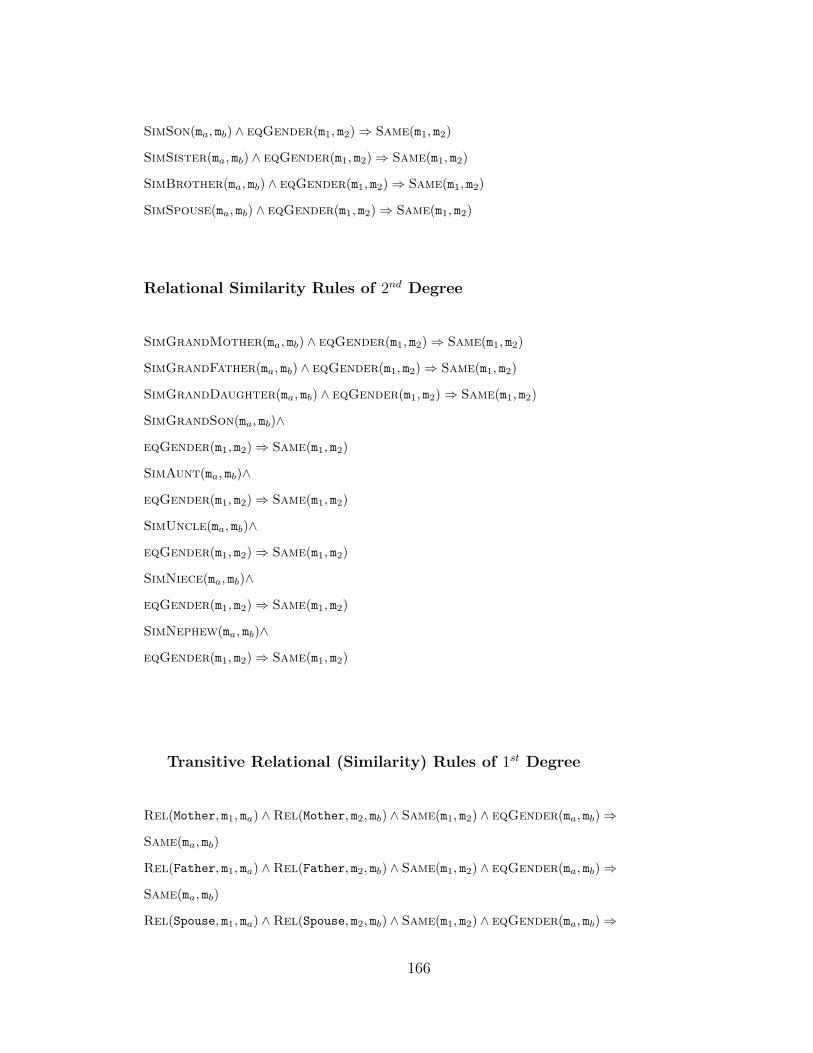
SimSon(ma, mb) ∧ eqGender(m1, m2)⇒ Same(m1, m2)

SimSister(ma, mb) ∧ eqGender(m1, m2)⇒ Same(m1, m2)

SimBrother(ma, mb) ∧ eqGender(m1, m2)⇒ Same(m1, m2)

SimSpouse(ma, mb) ∧ eqGender(m1, m2)⇒ Same(m1, m2)

Relational Similarity Rules of 2nd Degree

SimGrandMother(ma, mb) ∧ eqGender(m1, m2)⇒ Same(m1, m2)

SimGrandFather(ma, mb) ∧ eqGender(m1, m2)⇒ Same(m1, m2)

SimGrandDaughter(ma, mb) ∧ eqGender(m1, m2)⇒ Same(m1, m2)

SimGrandSon(ma, mb)∧

eqGender(m1, m2)⇒ Same(m1, m2)

SimAunt(ma, mb)∧

eqGender(m1, m2)⇒ Same(m1, m2)

SimUncle(ma, mb)∧

eqGender(m1, m2)⇒ Same(m1, m2)

SimNiece(ma, mb)∧

eqGender(m1, m2)⇒ Same(m1, m2)

SimNephew(ma, mb)∧

eqGender(m1, m2)⇒ Same(m1, m2)

Transitive Relational (Similarity) Rules of 1st Degree

Rel(Mother, m1, ma) ∧Rel(Mother, m2, mb) ∧ Same(m1, m2) ∧ eqGender(ma, mb)⇒

Same(ma, mb)

Rel(Father, m1, ma) ∧Rel(Father, m2, mb) ∧ Same(m1, m2) ∧ eqGender(ma, mb)⇒

Same(ma, mb)

Rel(Spouse, m1, ma) ∧Rel(Spouse, m2, mb) ∧ Same(m1, m2) ∧ eqGender(ma, mb)⇒

166

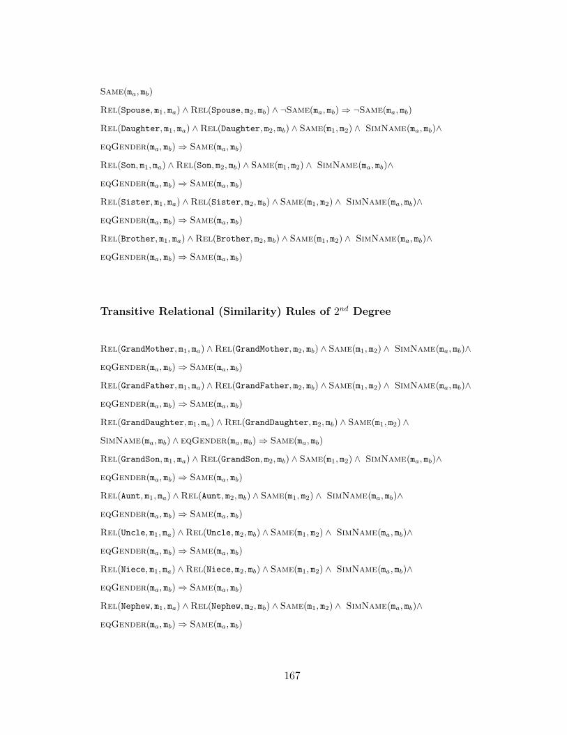
Same(ma, mb)

Rel(Spouse, m1, ma) ∧Rel(Spouse, m2, mb) ∧ ¬Same(ma, mb)⇒ ¬Same(ma, mb)

Rel(Daughter, m1, ma) ∧Rel(Daughter, m2, mb) ∧ Same(m1, m2) ∧ SimName(ma, mb)∧

eqGender(ma, mb)⇒ Same(ma, mb)

Rel(Son, m1, ma) ∧Rel(Son, m2, mb) ∧ Same(m1, m2) ∧ SimName(ma, mb)∧

eqGender(ma, mb)⇒ Same(ma, mb)

Rel(Sister, m1, ma) ∧Rel(Sister, m2, mb) ∧ Same(m1, m2) ∧ SimName(ma, mb)∧

eqGender(ma, mb)⇒ Same(ma, mb)

Rel(Brother, m1, ma) ∧Rel(Brother, m2, mb) ∧ Same(m1, m2) ∧ SimName(ma, mb)∧

eqGender(ma, mb)⇒ Same(ma, mb)

Transitive Relational (Similarity) Rules of 2nd Degree

Rel(GrandMother, m1, ma) ∧Rel(GrandMother, m2, mb) ∧ Same(m1, m2) ∧ SimName(ma, mb)∧

eqGender(ma, mb)⇒ Same(ma, mb)

Rel(GrandFather, m1, ma) ∧Rel(GrandFather, m2, mb) ∧ Same(m1, m2) ∧ SimName(ma, mb)∧

eqGender(ma, mb)⇒ Same(ma, mb)

Rel(GrandDaughter, m1, ma) ∧Rel(GrandDaughter, m2, mb) ∧ Same(m1, m2) ∧

SimName(ma, mb) ∧ eqGender(ma, mb)⇒ Same(ma, mb)

Rel(GrandSon, m1, ma) ∧Rel(GrandSon, m2, mb) ∧ Same(m1, m2) ∧ SimName(ma, mb)∧

eqGender(ma, mb)⇒ Same(ma, mb)

Rel(Aunt, m1, ma) ∧Rel(Aunt, m2, mb) ∧ Same(m1, m2) ∧ SimName(ma, mb)∧

eqGender(ma, mb)⇒ Same(ma, mb)

Rel(Uncle, m1, ma) ∧Rel(Uncle, m2, mb) ∧ Same(m1, m2) ∧ SimName(ma, mb)∧

eqGender(ma, mb)⇒ Same(ma, mb)

Rel(Niece, m1, ma) ∧Rel(Niece, m2, mb) ∧ Same(m1, m2) ∧ SimName(ma, mb)∧

eqGender(ma, mb)⇒ Same(ma, mb)

Rel(Nephew, m1, ma) ∧Rel(Nephew, m2, mb) ∧ Same(m1, m2) ∧ SimName(ma, mb)∧

eqGender(ma, mb)⇒ Same(ma, mb)

167

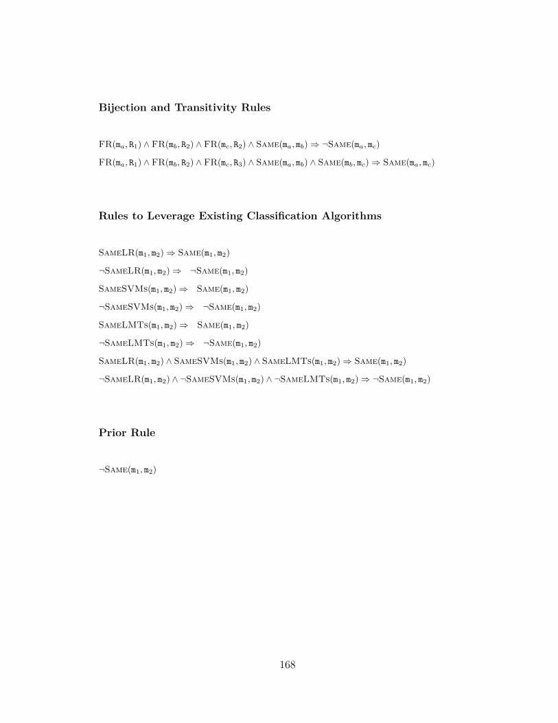
Bijection and Transitivity Rules

FR(ma, R1) ∧ FR(mb, R2) ∧ FR(mc, R2) ∧ Same(ma, mb)⇒ ¬Same(ma, mc)

FR(ma, R1) ∧ FR(mb, R2) ∧ FR(mc, R3) ∧ Same(ma, mb) ∧ Same(mb, mc)⇒ Same(ma, mc)

Rules to Leverage Existing Classification Algorithms

SameLR(m1, m2)⇒ Same(m1, m2)

¬SameLR(m1, m2)⇒ ¬Same(m1, m2)

SameSVMs(m1, m2)⇒ Same(m1, m2)

¬SameSVMs(m1, m2)⇒ ¬Same(m1, m2)

SameLMTs(m1, m2)⇒ Same(m1, m2)

¬SameLMTs(m1, m2)⇒ ¬Same(m1, m2)

SameLR(m1, m2) ∧ SameSVMs(m1, m2) ∧ SameLMTs(m1, m2)⇒ Same(m1, m2)

¬SameLR(m1, m2) ∧ ¬SameSVMs(m1, m2) ∧ ¬SameLMTs(m1, m2)⇒ ¬Same(m1, m2)

Prior Rule

¬Same(m1, m2)

168

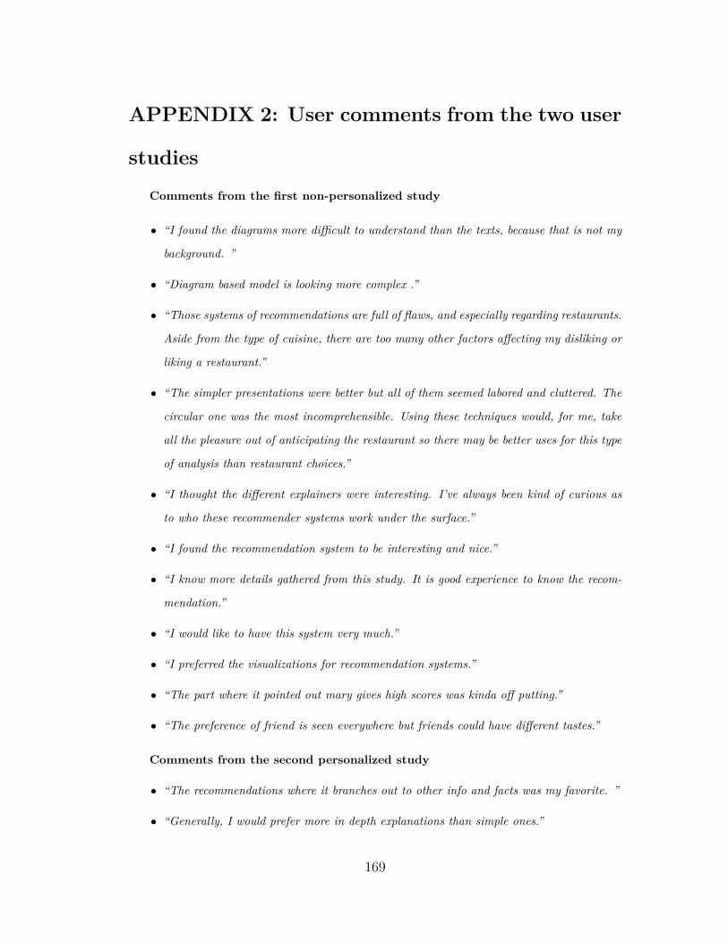
APPENDIX 2: User comments from the two user

studies

Comments from the first non-personalized study

• “I found the diagrams more difficult to understand than the texts, because that is not my

background. ”

• “Diagram based model is looking more complex .”

• “Those systems of recommendations are full of flaws, and especially regarding restaurants.

Aside from the type of cuisine, there are too many other factors affecting my disliking or

liking a restaurant.”

• “The simpler presentations were better but all of them seemed labored and cluttered. The

circular one was the most incomprehensible. Using these techniques would, for me, take

all the pleasure out of anticipating the restaurant so there may be better uses for this type

of analysis than restaurant choices.”

• “I thought the different explainers were interesting. I’ve always been kind of curious as

to who these recommender systems work under the surface.”

• “I found the recommendation system to be interesting and nice.”

• “I know more details gathered from this study. It is good experience to know the recom-

mendation.”

• “I would like to have this system very much.”

• “I preferred the visualizations for recommendation systems.”

• “The part where it pointed out mary gives high scores was kinda off putting.”

• “The preference of friend is seen everywhere but friends could have different tastes.”

Comments from the second personalized study

• “The recommendations where it branches out to other info and facts was my favorite. ”

• “Generally, I would prefer more in depth explanations than simple ones.”

169

• “Avoid venn diagrams.....they are never appealing.”

• “I think that it is a good platform to find music and people with the same taste in music.”

• “I liked when the categories like pop, rock or alternative are included in the recommenda-

tion. That would help with the choice to click on one.”

• “I don’t think the high volume of listening is a good factor since many artists that I like

are not high profile big bands, for instance, Iron Butterfly, and 10 years After. These

groups are not as popular as Led Zeppelin, but fit my music tastes.”

• “I think that the explanation tree is very unique and helpful.”

• “I liked the trees presentation - it looked good and was simple and made me feel involved

in the decision-making process.”

• “I really like the diagrams. Especially the overlapping circles. The branching tree was

good too. While I"m not sure I’ll use the service the idea for showing recommendations

is great!”

• “I liked the Venn diagram best for this type of information! It was fairly unique.”

• “I might not be in the majority, but my tastes are very eclectic. As such, I feel that just

because I listen to Band A and Band B doesn’t mean others will like both. Since my tastes

aren’t well matched I’m less likely to be convinced when a platform says that “User A and

myself both like Band A, and User A likes Band B, I’ll like Band B.””

• “I feel that the diagrams were overall better options to persuade people and myself of the

music recommendations. It would be more persuasive if it used more comparisons, i.e this

band is similar to these other 5 bands or people who liked this band also liked)”

• “I think that the recommendations were on point. It is especially important that peo-

ple aren’t overwhelmed with information, and I think the simple graphs provide the best

presentation to the end user.”

• “I thought the live recommendation system was pretty cool. I’d probably use a tool like

that to find new music. I also didn’t experience any technical issues.”

• “I think there are probably characteristics of individual tracks/songs that people are at-

tracted to which might vary less than variation within artist.”

170

• “I think the technology you use to recommend artists is very interesting and accurate!”

• “Seems there is too much algorithms and data analysis designed in recommending music

and artists to users. Music is inherently a subjective thing so I’m not sure I think this is

the best method.”

• “I prefer text best rather than diagrams for recommendations.”

• “The last option of recommendation system (tree with orange dots) was similar to the

first, but I didn’t like it as much because you had to click each dot to get the information,

where it just presented to you quickly in the first option. The Venn diagram was pretty

confusing. The text descriptions work, but don’t carry the weight of having the graphical

recommendations.”

• “The tagged as data doesn’t really work for me in this instance. “seen live” does nothing

for me. I like the visual feedback though. ”

171