Embed Size (px)
Citation preview
Resonance Behavior of Magnetostrictive Sensor in Longitudinal Vibration mode for
Biological Agent Detection
by
Madhumidha Ramasamy
A thesis submitted to the Graduate Faculty of
Auburn University
in partial fulfillment of the
requirements for the Degree of
Master of Science
Auburn, Alabama
December 13, 2010
Keywords: Magnetostriction, Longitudinal Vibration mode, Biological Agent Detection,
Numerical Simulation and Resonance Behavior
Copyright 2010 by Madhumidha Ramasamy
Approved by
Bart C. Prorok, Chair, Associate Professor of Materials Engineering
Dong-Joo Kim, Associate Professor of Materials Engineering
Pradeep Lall, Professor of Mechanical Engineering
ii
Abstract
The growing threat of bio warfare agents and bioterrorism has led to the development of
specific field tools that perform rapid analysis and identification of encountered suspect
materials. One such technology, recently developed is a micro scale acoustic sensor that uses
experimental modal analysis. Ferromagnetic materials with the property to change their physical
dimensions in response to changing its magnetization can be built into such sensors and
actuators. One such sensor is fashioned from Metglas 2826MB, a Magnetostrictive strip actuated
in their longitudinal vibration mode when subjected to external magnetic field. Due to mass
addition, these magnetostrictive strips are driven to resonance with a modulated magnetic field
resulting in frequency shifts. In Vibration Mechanics the frequency shift for a certain amount of
mass will have a tolerance limit based on their distribution and discrete position over the sensor
platform. In addition, lateral positioning of same amount of mass does not influence the resonant
frequency shift of the sensor. This work concentrates on developing a model correlating
theoretical, experimental and numerical simulations to determine the mass of E. Coli O157:H7
cells attached to the sensor platform

iii
Acknowledgments
I would like to sincerely thank my mentor, Dr. Bart C. Prorok without whom none of this
would have been possible. His continuous support, encouragement and valuable suggestions
played a vital role in the achievement of this research. I would like to extend my thanks to my
advisory committee members, Dr. Dong-joo Kim and Dr. Pradeep Lall for their participation in
my thesis committee. I would like thank Mr. Charles Ellis for his financial support in my final
semester which was great timely help. I would also like to thank my Research mates Cai, Shaqib,
Dong, Bo, Kevin, Nicole and Brandon for their constant support and encouragement during the
course of my work.
I take immense pleasure in thanking my family members for believing in me and standing
by me at every step till today. Special thanks to Nida for being my strength and making me feel
auburn as home away from home. Finally I would like to thank all my friends for their
unwavering support and timely help.
iv
Table of Contents
Abstract ......................................................................................................................................... ii
Acknowledgments........................................................................................................................ iii
List of Figures .............................................................................................................................. vi
List of Tables ............................................................................................................................... ix
Chapter 1 Introduction .................................................................................................................. 1
1.1 Motivation for Research ........................................................................................... 1
1.2 Overview ................................................................................................................... 5
Chapter 2 Literature Review ........................................................................................................ 6
2.1 Available Techniques for Bio Species Detection ...................................................... 6
2.1.1 Electro-Chemical Sensors ................................................................................. 8
2.1.2 Optical Sensors ................................................................................................ 9
2.1.3 Mass Sensors ................................................................................................... 12
2.1.3.1 QCM ................................................................................................... 12
2.1.3.2 SAW .................................................................................................... 13
2.1.3.3 Micro cantilever .................................................................................. 14
2.2 Magnetostrictive Sensors .......................................................................................... 16
2.2.1 Metglas 2628 MB ........................................................................................... 17
2.3 Detection of Escherichia coli.................................................................................... 19
Chapter 3 Materials and Methods ............................................................................................... 21
v
3.1 Magnetostriction ....................................................................................................... 21
3.2 Longitudinal Vibration Mode ................................................................................... 22
3.3 Principle of Operation ............................................................................................... 23
3.4 Design and Numerical Simulation ............................................................................ 28
3.5 Experimental Method................................................................................................ 30
3.5.1 Glass Bead Attachment ................................................................................... 32
3.5.2 Detection Setup ............................................................................................... 33
Chapter 4 Results and Discussion ............................................................................................... 35
4.1 Distribution of Mass ................................................................................................. 35
4.1.1 Uniform Distribution ....................................................................................... 36
4.1.2 Non-uniform Distribution ................................................................................ 38
4.1.2.1 Maximum Frequency Shift .................................................................. 39
4.1.2.2 Minimum Frequency Shift ................................................................... 46
4.2 Influence of Discrete Position .................................................................................... 54
4.2.1 Simulation Result .............................................................................................. 54
4.2.2 Experimental Result .......................................................................................... 55
4.2.3 Theoretical Verification .................................................................................... 56
4.3 Influence of Physical Dimension .............................................................................. 59
4.3.1 Length Dependence .......................................................................................... 59
4.3.2 Width Dependence ............................................................................................ 61
Chapter 5 Conclusion .................................................................................................................. 62
References ................................................................................................................................. 63
vi
List of Figures
Figure 1.1 Comparative toxicity of effective doses of biological agents, toxins, and chemical
agents bacteria .............................................................................................................................. 2
Figure 1.2 Distributions, by industry of application, of the relative number of works
appeared in the literature on detection of pathogenic bacteria .................................................... 3
Figure 1.3 Distribution, by micro-organism, of the relative number of works appeared in the
literature on detection of pathogenic bacteria .............................................................................. 4
Figure 2.1 Approximate numbers of articles using different techniques to detect and/or
identify pathogenic bacteria ......................................................................................................... 6
Figure 2.2 Schematic diagram of typical transduction formats employed in biosensors ............ 7
Figure 2.3 Diagram of how an amperometric immunofiltration biosensor works ...................... 9
Figure 2.4 Schematic diagram of a biosensor utilizing surface plasmon resonance (SPR)
transduction ................................................................................................................................. 10
Figure 2.5 Schematic diagram of a biosensor based on piezoelectric transduction ................... 12
Figure 2.6 Schematic diagram of a micro cantilever-based biosensor ...................................... 15
Figure 2.7 Magnetostrictive strips used on valued goods for theft protection ........................... 17
Figure 3.1 SEM images of the Magnetoelastic strips by simple micro fabrication technique .. 18
Figure 3.2 SEM image of E. coli O157:H7 cells ....................................................................... 20
Figure 3.3 Schematics of a magnetostrictive sensor’s response to the applied magnetic........... 21
Figure 3.4 Transverse vs. longitudinal actuation illustrated with a freestanding
magnetostrictive strips ................................................................................................................ 23
Figure 3.5 Mechanical force analysis in a unit of sensor ........................................................... 24
Figure 3.6 Schematic of sensor structure in beam ..................................................................... 25
Figure 3.7 Effect of Mass attachment on the wave speed of the sensor platform due to
longitudinal vibration ................................................................................................................. 27
vii
Figure 3.8 Simulation result of a 250 µm x 50 µm x 4 µm sensor meshed with equilateral
triangle facets of element size 7.5 µm......................................................................................... 28
Figure 3.9 Simulation results for freestanding Metglas beam with the size of 250 µm x 50
µm x 4 µm. Poisson’s ratio of 0.33 was employed .................................................................... 29
Figure 3.10 Procedural steps involved in the Micro fabrication of Magnetostrictive strips for
the sensor platform ...................................................................................................................... 31
Figure 3.11 SEM images showing glass beads attached to the sensor in various locations ....... 32
Figure 3.12 Resonant frequency detection setup containing Actuation/read coil, and
magnetic bar ............................................................................................................................... 33
Figure 4.1 SEM image of the sensor platform with the uniform distribution of E.coli cells
attached experimentally ............................................................................................................. 35
Figure 4.2 Resonant Frequency Shift due to uniform distribution of E.coli cells ..................... 37
Figure 4.3 SEM image of a sensor with Non-Uniform distribution of E.coli cells ................... 38
Figure 4.4 Schematic diagrams representing the non-uniform distribution for the maximum
resonant frequency condition ..................................................................................................... 39
Figure 4.5 Plots representing the Maximum Resonant Frequency Shift due to Non-uniform
and Uniform distribution of E.coli cells .................................................................................... 44
Figure 4.6 Plots representing the Maximum Resonant Frequency Shift due to Non-uniform
distribution of E.coli cells for Numerical Simulation and theoretically calculated results ....... 46
Figure 4.7 Schematic diagrams representing the non-uniform distribution for the minimum
resonant frequency condition ...................................................................................................... 47
Figure 4.8 Plots representing the Minimum Resonant Frequency Shift due to Non-uniform
and Uniform distribution of E.coli cells .................................................................................... 49
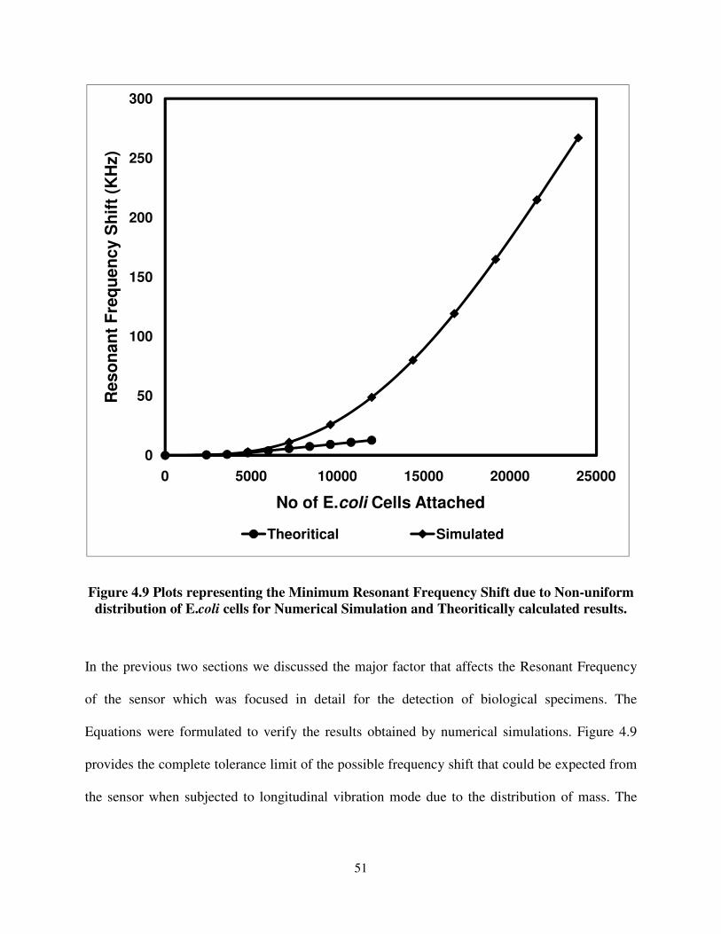
Figure 4.9 Plots representing the Minimum Resonant Frequency Shift due to Non-uniform
distribution of E.coli cells for Numerical Simulation and theoretically calculated results ....... 51
Figure 4.10 Plots representing the Resonant Frequency Shift of the sensor platform of
dimension 250µm x 50µm x 4µm due to distribution of mass (E.coli cells of size 1.43µm x
0.73µm x 0.73µm.) .................................................................................................................... 52
Figure 4.11 Addition of concentrated mass at discrete location x on the sensor platform of
length L ...................................................................................................................................... 53
Figure 4.12 Plots of Resonant Frequency shift in KHz for the addition of concentrated mass
at discrete locations over the sensor platform ............................................................................ 57
Figure 4.13 Plots of Resonant Frequency shift due to mass distribution over the sensor
platform with varying Length ..................................................................................................... 59

viii
Figure 4.14 Plots of Resonant Frequency shift due to mass distribution over the sensor
platform with varying Width ..................................................................................................... 60
ix
List of Tables
Table 4.1 Reseonant Frequency shift due to uniform distribution of E.coli cells over the
sensor platform ........................................................................................................................... 36
Table 4.2 Calculated values of η and KL with the corresponding resonant frequency shift
values determined using the Equation (4.12) and (3.6) ............................................................. 43
Table 4.3 Calculated and Simulated Maximum Resonant Frequency Shift results for Non-
Uniform Distribution ................................................................................................................. 45
Table 4.4 Calculated values of η and KL with the corresponding resonant frequency shift
values determined using the Equation (4.14) and (3.6) ............................................................. 48
Table 4.5 Calculated and Simulated Minimum Resonant Frequency Shift results for Non-
Uniform Distribution ................................................................................................................. 50
Table 4.6 Test results of sensor (5 mm x 1 mm x 28 µm) attached with glass bead at
different locations ...................................................................................................................... 54
Table 4.7 The Resonant Frequency values corresponding to concentrated mass on discrete
locations ..................................................................................................................................... 57
1
CHAPTER 1
INTRODUCTION
1.1. Motivation For Research
The end of cold war has reduced international tension between the super powers. However,
there has been a remarkable increase in the production and availability of chemical and
biological weapons throughout the world. The combination of these factors has significantly
increased the possibility of an attack on the human race involving the use of such weapons.
Biological agents are often considered to be psychologically more threatening of the two, and
therefore provide more appeal to the terrorist[1]. Biological agents can be manufactured in
facilities that are inexpensive to construct; that resemble pharmaceutical, food, or medical
production sites; and that provide no detectable sign that such agents are being produced. One
characteristic of biological agents that makes them so attractive to potential users is their
remarkably low effective dose; that is, the mass of agent that is required to create the desired
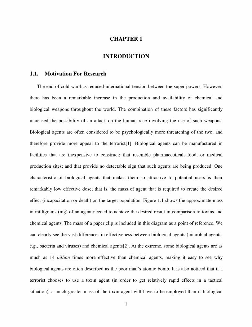
effect (incapacitation or death) on the target population. Figure 1.1 shows the approximate mass
in milligrams (mg) of an agent needed to achieve the desired result in comparison to toxins and
chemical agents. The mass of a paper clip is included in this diagram as a point of reference. We
can clearly see the vast differences in effectiveness between biological agents (microbial agents,
e.g., bacteria and viruses) and chemical agents[2]. At the extreme, some biological agents are as
much as 14 billion times more effective than chemical agents, making it easy to see why
biological agents are often described as the poor man’s atomic bomb. It is also noticed that if a
terrorist chooses to use a toxin agent (in order to get relatively rapid effects in a tactical
situation), a much greater mass of the toxin agent will have to be employed than if biological
2
agents were being used. This mass of toxin agent in some cases may be equivalent to chemical
agent masses.
Figure 1.1 Comparative toxicity of effective doses of biological agents, toxins, and chemical
agents[1]
Bacteria are small, single-celled organisms, most of which can be grown on solid or in liquid
culture media. Under special circumstances, some types of bacteria can transform into spores
that are more resistant to cold, heat, drying, chemicals, and radiation than the bacterium itself.
Most bacteria do not cause disease in human beings, but those that do cause disease act in two
differing mechanisms: by invading the tissues or by producing poisons (toxins). Many bacteria,
such as anthrax, have properties such as Retained potency during growth and processing to the
end product (biological weapon), Long “shelf-life.”, · Low biological decay as an aerosol that
makes them attractive as potential warfare agents [1-3].
3
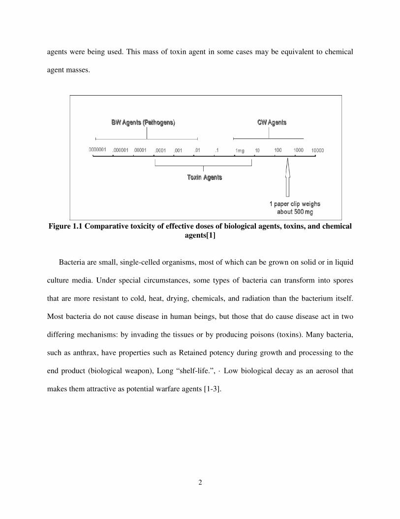
Figure 1.2 Distributions, by industry of application, of the relative number of works
appeared in the literature on detection of pathogenic bacteria[3].
Biological agents are effective in very low doses. Therefore, biological agent detection systems
need to exhibit high sensitivity (i.e., be able to detect very small amounts of biological agents).
The complex and rapidly changing environmental background also requires these detection
systems to exhibit a high degree of selectivity (i.e., be able to discriminate biological agents
from other harmless biological and non-biological material present in the environment). A third
challenge that needs to be addressed is speed or response. One other problem facing the
production of biosensors for direct detection of bacteria is the sensitivity of assay in real samples.
The infectious dosages of pathogens such as Salmonella or E. coli O157:H7 is 10 cells and the
existing coli form standard for E. coli in water is 4 cells: 100 ml. Hence, a biosensor must be able
to provide a detection limit as low as single coli form organism in 100 ml of potable water, with
a rapid analysis time at a relatively low cost. Only in this case will the biosensor be convenient
4
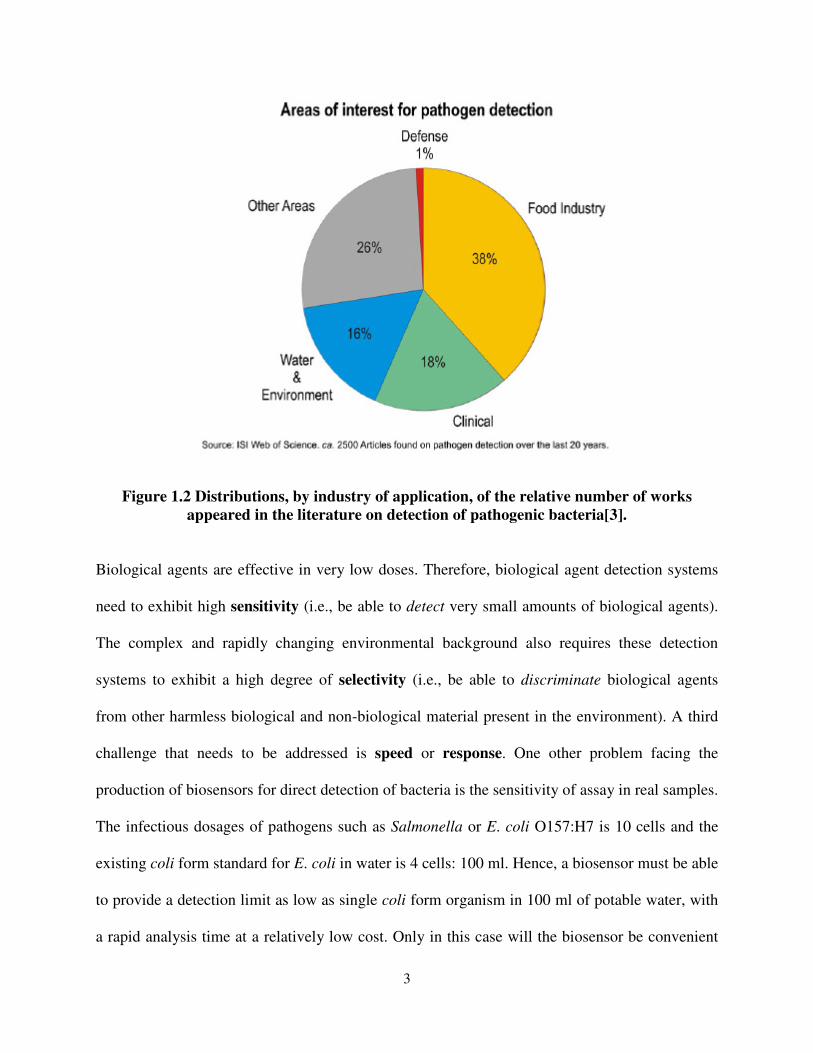
for on-line testing of bacterial pathogens in real samples. Thus, sensitivity is another issue that
still requires improvement. There is also a problem of distinguishing between live and dead cells
[4-6].
Figure 1.3 Distribution, by micro-organism, of the relative number of works appeared in
the literature on detection of pathogenic bacteria[3].
These combined requirements provide a significant technical challenge. Additionally, there
has been limited development in the area of biological agent detection equipment in the
commercial market (i.e., hand-held devices). There are several detection systems being
developed and tested by the military that show promise. However, these systems are relatively
complicated, require training for successful operation and maintenance, and are expensive to
purchase and operate. It is expected that over the course of the next 5 years, commercial
instrumentation, hardened for use in the field, may become available at reasonable costs. This
eventually leads us to focus our research on developing biological agents’ detection techniques

5
that are very rapid, sensitive and cost effective. Traditionally, infectious agents were detected
and identified using standard microbiological and biochemical assays that were accurate but
time-consuming. New techniques are needed that combine the accuracy and breadth of
traditional microbiological approaches with the improved accuracy and sensitivity[7, 8].
1.2. Overview
The aim of this work is to develop Mass sensors for the detection of biological agents that are
hazardous to human life. The current chapter gives the motivation and overview of the
organization of study. Next chapter briefs the importance of biosensors and the various types of
biosensors that are more emphasized for the detection of biological agents. The various
categories are briefly explained with merits and demerits that lead to our research work on the
mass sensor made of magnetostrictive strip for the detection process. The chapter also explains
the biological pathogen that we focused for our research work and its effects on human life.
Chapter 3 portrays the details of the materials and methods involved in the development of the
sensor platform. It also includes the theoretical derivation for the determination of the resonance
behavior of the sensor due to various mass related distribution conditions. The experimental
details also include the numerical specifications and the schematic set up for the detection of the
pathogens. Chapter 4 presents the results and discussions of the project describing the factors
affecting the resonance behavior of the sensor platform due addition of pathogens as mass and
their varsity of distributions. Chapter 5 summarizes the conclusions and potential future work of
this study.
6
CHAPTER 2
LITERATURE REVIEW
2.1 Techniques for Pathogens Detection
Amongst the growing areas of interest, the use of rapid methods for defense applications
stands out In fact, the number of publications dealing with these applications already account for
over 1% of all publications in the field of rapid methods for pathogen detection since 1985. The
food industry is the main party concerned with the presence of pathogenic bacteria. The public
health implications of failing to detect certain bacteria can be fatal, and the consequences easily
make the news. The following sections describe the various approaches most commonly taken to
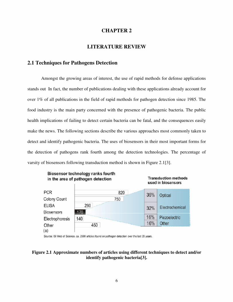
detect and identify pathogenic bacteria. The uses of biosensors in their most important forms for
the detection of pathogens rank fourth among the detection technologies. The percentage of
varsity of biosensors following transduction method is shown in Figure 2.1[3].
Figure 2.1 Approximate numbers of articles using different techniques to detect and/or
identify pathogenic bacteria[3].
7
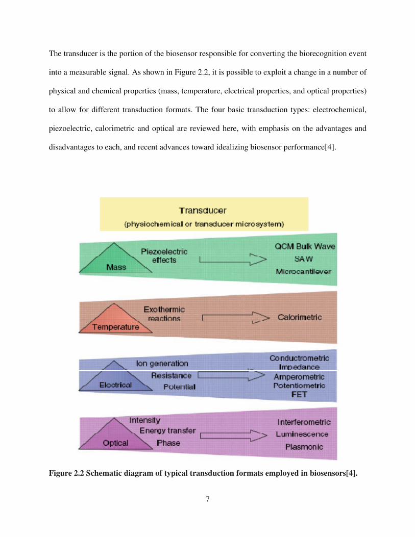
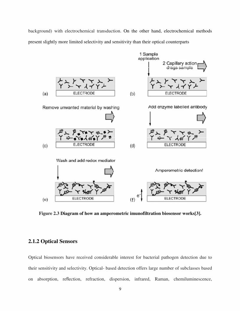
The transducer is the portion of the biosensor responsible for converting the biorecognition event
into a measurable signal. As shown in Figure 2.2, it is possible to exploit a change in a number of
physical and chemical properties (mass, temperature, electrical properties, and optical properties)
to allow for different transduction formats. The four basic transduction types: electrochemical,
piezoelectric, calorimetric and optical are reviewed here, with emphasis on the advantages and
disadvantages to each, and recent advances toward idealizing biosensor performance[4].
Figure 2.2 Schematic diagram of typical transduction formats employed in biosensors[4].
8
2.1.1 Electrochemical Sensors
Electrochemical transduction is one of the most popular transduction formats employed in
biosensing applications. One of the main advantages of biosensors which employ
electrochemical transduction is the ability to operate in turbid media and often in complex
matrices. Another distinct advantage of electrochemical transduction is that the detection
components are inexpensive and can be readily miniaturized into portable, low cost devices. In
general, electrochemical-based sensing can be divided into three main categories, potentiometric,
amperometric, and impedance. Potentiometric sensors typically rely on a change in potential
caused by the production of an electro active species that is measured by an ion selective
electrode. For a biosensor system, this change in electro active species concentration is usually
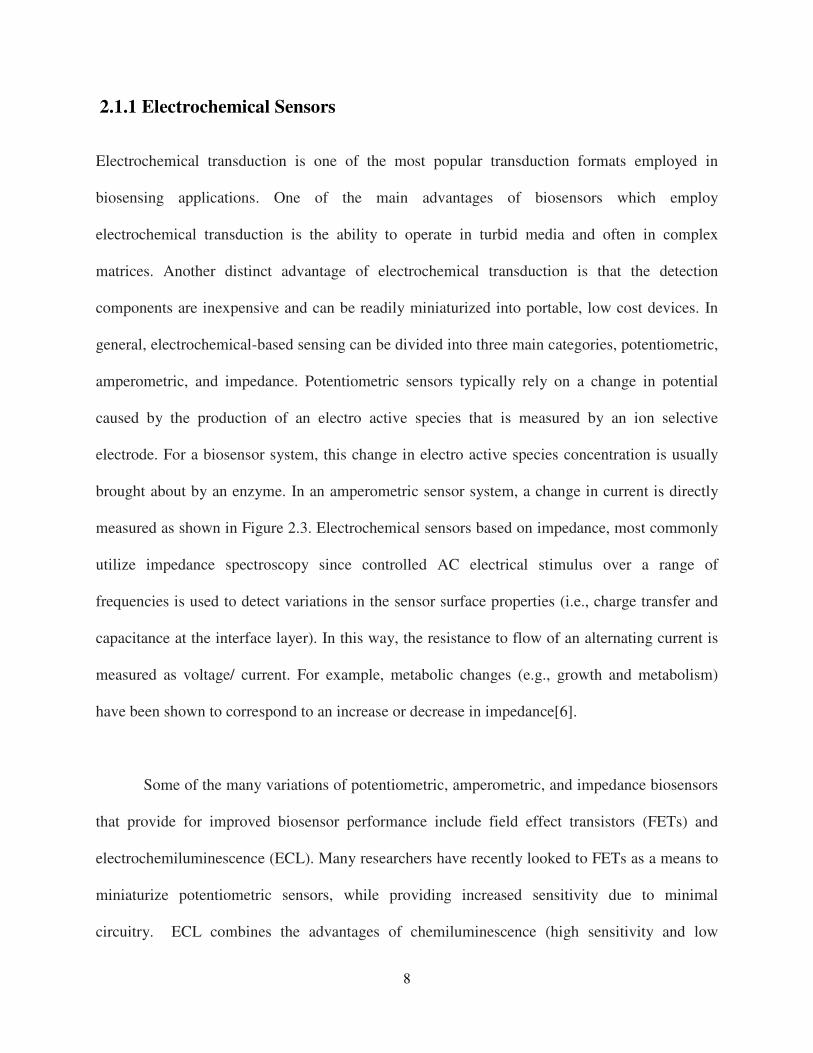
brought about by an enzyme. In an amperometric sensor system, a change in current is directly
measured as shown in Figure 2.3. Electrochemical sensors based on impedance, most commonly
utilize impedance spectroscopy since controlled AC electrical stimulus over a range of
frequencies is used to detect variations in the sensor surface properties (i.e., charge transfer and
capacitance at the interface layer). In this way, the resistance to flow of an alternating current is
measured as voltage/ current. For example, metabolic changes (e.g., growth and metabolism)
have been shown to correspond to an increase or decrease in impedance[6].
Some of the many variations of potentiometric, amperometric, and impedance biosensors
that provide for improved biosensor performance include field effect transistors (FETs) and
electrochemiluminescence (ECL). Many researchers have recently looked to FETs as a means to
miniaturize potentiometric sensors, while providing increased sensitivity due to minimal
circuitry. ECL combines the advantages of chemiluminescence (high sensitivity and low
9
background) with electrochemical transduction. On the other hand, electrochemical methods
present slightly more limited selectivity and sensitivity than their optical counterparts
Figure 2.3 Diagram of how an amperometric imunofiltration biosensor works[3].
2.1.2 Optical Sensors
Optical biosensors have received considerable interest for bacterial pathogen detection due to
their sensitivity and selectivity. Optical- based detection offers large number of subclasses based
on absorption, reflection, refraction, dispersion, infrared, Raman, chemiluminescence,
10
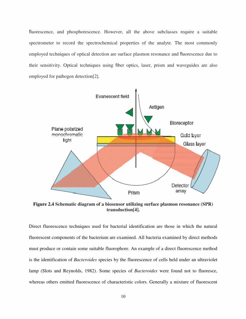
fluorescence, and phosphorescence. However, all the above subclasses require a suitable
spectrometer to record the spectrochemical properties of the analyte. The most commonly
employed techniques of optical detection are surface plasmon resonance and fluorescence due to
their sensitivity. Optical techniques using fiber optics, laser, prism and waveguides are also
employed for pathogen detection[2].
Figure 2.4 Schematic diagram of a biosensor utilizing surface plasmon resonance (SPR)
transduction[4].
Direct fluorescence techniques used for bacterial identification are those in which the natural
fluorescent components of the bacterium are examined. All bacteria examined by direct methods
must produce or contain some suitable fluorophore. An example of a direct fluorescence method
is the identification of Bacteroides species by the fluorescence of cells held under an ultraviolet
lamp (Slots and Reynolds, 1982). Some species of Bacteroides were found not to fluoresce,
whereas others emitted fluorescence of characteristic colors. Generally a mixture of fluorescent
11
metabolic products is detected. In many schemes used in the clinical environment, fluorescence
is detected visually while the sample is held under a UV lamp. This approach has the advantages
of simplicity, low cost, and rapidity. However, there is at least one major limitation to the utility
of direct methods. That is, only those bacteria which contain or produce some fluorescent
pigment may be examined. Therefore, the utility of this approach is very limited (Rossi and
Warner, 1985). SPR biosensors (Cooper, 2003) measure changes in refractive index caused by
structural alterations in the vicinity of a thin film metal surface. Current instruments operate as
shown in Figure 2.4. A glass plate covered by a gold thin film is irradiated from the backside by
p-polarized light (from a laser) via a hemispherical prism, and the reflectivity is measured as a
function of the angle of incidence, θ. The resulting plot is a curve showing a narrow dip. This
peak is known as the SPR minimum. The angle position of this minimum is determined by the
properties of the gold-solution interface. Hence, adsorption phenomena and even antigen–
antibody reaction kinetics can be monitored using this sensitive technique (as a matter of fact,
SPR is used to determine antigen–antibody affinity constants). The main drawbacks of this
powerful technique lay in its complexity (specialized staff is required), high cost of equipment
and large size of most currently available instruments. SPR has successfully been applied to the
detection of pathogen bacteria by means of immunoreactions (Taylor et al., 2005; Oh et al.,
2005a). Optical techniques perhaps provide better sensitivity than electrochemical ones, but their
cost and complexity makes them unattractive to most end users[2].
12
2.1.3 Mass Sensors
Biosensors that detect the change in mass due to target and biorecognition element interactions
predominately rely on piezoelectric transduction. Piezoelectric transduction relies on an
electrical charge produced by mechanical stress, which is correlated to a biorecognition binding
event causing a change in the mass on the piezoelectric device. The main advantage to the
piezoelectric transduction (i.e., mass sensor) approach includes the ability to perform label-free
measurements of the binding events, including real-time analysis of binding kinetics[4].
2.1.3.1 Quartz Crystal Microbalance Sensors
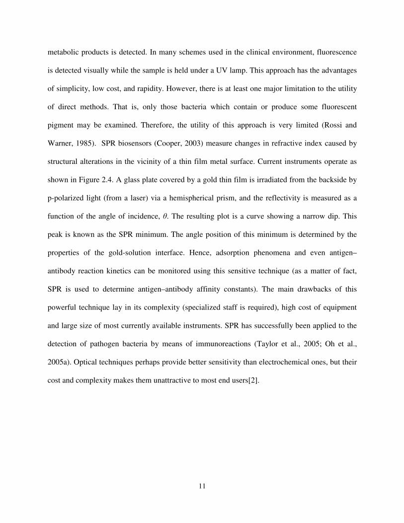
The most commonly employed transducer is the quartz crystal microbalance (QCM),
which relies on a bulk wave effect, illustrated in Figure 2.5. A QCM device consists of a quartz
disk that is plated with electrodes.
Figure 2.5 Schematic diagram of a biosensor based on piezoelectric transduction[4].
13
Upon introduction of an oscillating electric field, an acoustic wave propagates across the
device. The change in mass associated with bioreceptor–target interactions causes a decrease in
the oscillation frequency that is directly proportional to the amount of target. This transduction
format can be coupled to a wide variety of bioreceptors (e.g., antibody, aptamer, and imprinted
polymer), provided that the mass change is large enough to produce a measurable change in
signal. Not surprisingly, QCM transduction is not capable of small molecule detection directly,
and usually requires some sort of signal amplification to be employed. A disadvantage of PZ
sensors is the relatively long incubation time of the bacteria, the numerous washing and drying
steps, and the problem of regeneration of the crystal surface. This last problem may not be
important if small crystals can be manufactured at low cost so that disposable transducers are
economically feasible. Possible limitations of this technology include also the lack of specificity,
sensitivity and interferences from the liquid media where the analysis takes place[9].
2.1.3.2 Surface Acoustic Wave Sensors
Changes in the overall mass of the biomolecular system due to association of the
bioreceptor with the target analyte can be measured using alternative piezoelectric transducer
devices that offer some advantages over bulk wave sensing. For example, surface acoustic wave
(SAW) devices exhibit increased sensitivity compared to bulk wave devices and transmit along a
single crystal face, where the electrodes are located on the same side of the crystal and the
transducer acts as both a transmitter and a receiver. SAW devices can directly sense changes in
mass due to binding interactions between the immobilized bioreceptor and target analytes and
14
exhibit increased sensitivity compared to bulk wave devices. However, the acoustic wave is
significantly dampened in biological solutions, limiting its utility for biosensing applications.
Some improvements using dual channel devices, and special coated electrode systems allowing
for noncontact SAW devices, which can function in biological solution interfaces have been
produced. However, reliable biosensor application incorporating these devices is still under
pursuit, as improvements in sensitivity are still required for specific microbial analyses[9].
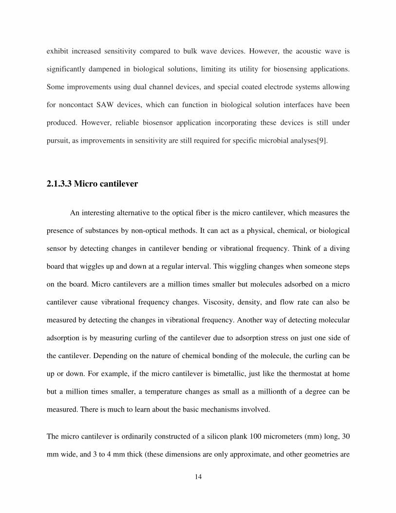
2.1.3.3 Micro cantilever
An interesting alternative to the optical fiber is the micro cantilever, which measures the
presence of substances by non-optical methods. It can act as a physical, chemical, or biological
sensor by detecting changes in cantilever bending or vibrational frequency. Think of a diving
board that wiggles up and down at a regular interval. This wiggling changes when someone steps
on the board. Micro cantilevers are a million times smaller but molecules adsorbed on a micro
cantilever cause vibrational frequency changes. Viscosity, density, and flow rate can also be
measured by detecting the changes in vibrational frequency. Another way of detecting molecular
adsorption is by measuring curling of the cantilever due to adsorption stress on just one side of
the cantilever. Depending on the nature of chemical bonding of the molecule, the curling can be
up or down. For example, if the micro cantilever is bimetallic, just like the thermostat at home
but a million times smaller, a temperature changes as small as a millionth of a degree can be
measured. There is much to learn about the basic mechanisms involved.
The micro cantilever is ordinarily constructed of a silicon plank 100 micrometers (mm) long, 30
mm wide, and 3 to 4 mm thick (these dimensions are only approximate, and other geometries are
15
sometimes used). When molecules are added to its surface, the extent to which the plank bends
can be measured accurately by bouncing a light beam off the surface and measuring the extent to
which the light beam is deflected. The vibrational frequency can be induced by piezoelectric
transducers and measured with t he same laser beam that measured the deflection because it
generates an alternating current in the detector[10].
Figure 2.6 Schematic diagram of a micro cantilever-based biosensor[4].
Yet another mechanism of response was employed to measure proteins in solution. Antibodies
were covalently attached to the silicon surface of a cantilever in such a way that the stresses
induced in the antibody when it reacted with its antigen were detected. Detection of biological
warfare agents or bacteria and viruses in the hospital laboratory should be expedited with this
16
stressed antibody technique. Additional experiments are under way to demonstrate the usefulness
of the microcantilever as a biosensor.
Because of the small size and versatility of the microcantilever, arrays of sensors can be
fabricated on a single chip to conceptually mimic the five sensory facilities: sight, hearing, smell,
taste, and touch. ORNL researchers Thomas Thundat, Bruce Warmack, Eric Wachter, Patrick
Oden, and Panos Datskos received a 1996 R&D 100 Award for development of the
microcantilever[11, 12].
2.2 Magnetostrictive Sensors
Recently, magnetoelastic sensor (ME) platform are gaining attention in chemical and
biological sensing. ME sensors are constructed with amorphous ferromagnetic ribbons or wires
which are analogous and complementary to piezoelectric acoustic wave sensors. ME sensors are
excited with magnetic AC fields and in turn, they generate magnetic fluxes that can be detected
with a sensing coil from a distance and hence these sensors are highly attractive for wireless
biosensing. They have high tensile strength and are much more cost effective which makes them
appealing for biosensor platform. The fundamental operating principle of the magnetoelastic
sensors involves a change in sensor resonance frequency due to mass loading of the sensor. In
biosensing, the change in mass is associated with the binding of a target analyte to a bioreceptor
immobilized on the surface of the ribbon-like ME sensor[13].
The ME sensor can be coated with various probe molecules to target analytes. A change
in resonant frequency can be observed if an analyte binds to the magnetoelastic sensor which can
be measured rapidly and accurately. Also, the cost of the sensor was approximately is very
17
cheap, therefore it can be easily utilized as a disposable sensor. Magnetoelastic sensor
information is by magnetic flux; hence, no direct connections are needed between the sensor and
monitoring electronic equipment making possible a variety of in situ and in vivo monitoring
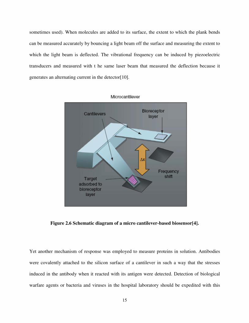
applications. Recently, ME biosensor are developed by immobilizing bacteriophage as
biorecognition element for the real-time in vitro detection of B. anthracis spores[14].
Figure 2.7 Magnetostrictive strips used on valued goods for theft protection
2.2.1 Metglas 2628mb
Ferromagnetic materials generally are Fe, Ni, and Co metals or their alloys. So far,
ferromagnetic materials have been demonstrated to be a good candidate for magnetostrictive
sensors because of their soft magnetic properties (low remanence and coercive field) in general.
Moreover, ferromagnetic material can be made in amorphous (non-crystalline) metallic alloys by
rapidly spinning and cooling of a liquid alloy. For example, Metglas 2826 MB [10], consisting of
Fe, Ni, Mo, and B, is a typical amorphous ferromagnetic material having the advantages of
nearly magnetic isotropic structure, considerable high permeability, low coercivity, and low
18
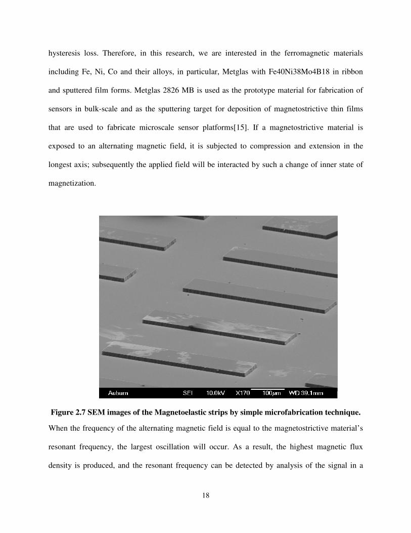
hysteresis loss. Therefore, in this research, we are interested in the ferromagnetic materials
including Fe, Ni, Co and their alloys, in particular, Metglas with Fe40Ni38Mo4B18 in ribbon
and sputtered film forms. Metglas 2826 MB is used as the prototype material for fabrication of
sensors in bulk-scale and as the sputtering target for deposition of magnetostrictive thin films
that are used to fabricate microscale sensor platforms[15]. If a magnetostrictive material is
exposed to an alternating magnetic field, it is subjected to compression and extension in the
longest axis; subsequently the applied field will be interacted by such a change of inner state of
magnetization.
Figure 2.7 SEM images of the Magnetoelastic strips by simple microfabrication technique.
When the frequency of the alternating magnetic field is equal to the magnetostrictive material’s
resonant frequency, the largest oscillation will occur. As a result, the highest magnetic flux
density is produced, and the resonant frequency can be detected by analysis of the signal in a
19
close loop circuit. This is the basis for antitheft sensor tags currently used Electronic Article
Surveillance (EAS) system [13, 16] and sensors used to measure chemical and biochemical
species. This study will further extend the applications of the magnetostrictive phenomena to
detecting mass loaded on magnetostrictive sensors.
2.3 Detection of Escherichia coli:
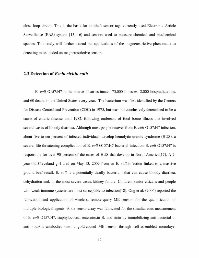
E. coli O157:H7 is the source of an estimated 73,000 illnesses, 2,000 hospitalizations,
and 60 deaths in the United States every year. The bacterium was first identified by the Centers
for Disease Control and Prevention (CDC) in 1975, but was not conclusively determined to be a
cause of enteric disease until 1982, following outbreaks of food borne illness that involved
several cases of bloody diarrhea. Although most people recover from E. coli O157:H7 infection,
about five to ten percent of infected individuals develop hemolytic uremic syndrome (HUS), a
severe, life-threatening complication of E. coli O157:H7 bacterial infection. E. coli O157:H7 is
responsible for over 90 percent of the cases of HUS that develop in North America[17]. A 7-
year-old Cleveland girl died on May 13, 2009 from an E. coli infection linked to a massive
ground-beef recall. E. coli is a potentially deadly bacterium that can cause bloody diarrhea,
dehydration and, in the most severe cases, kidney failure. Children, senior citizens and people
with weak immune systems are most susceptible to infection[18]. Ong et al. (2006) reported the
fabrication and application of wireless, remote-query ME sensors for the quantification of
multiple biological agents. A six-sensor array was fabricated for the simultaneous measurement
of E. coli O157:H7, staphylococcal enterotoxin B, and ricin by immobilizing anti-bacterial or
anti-biotoxin antibodies onto a gold-coated ME sensor through self-assembled monolayer
20
modification cross-linking the antibody with a bifunctional binding agent. The paper reported
that the telemetry of magnetoelastic sensor information is by magnetic flux; hence, no direct
connections are needed between the sensor and monitoring electronic equipment making
possible a variety of in situ and in vivo monitoring applications. Recently, Huang et al. (2008)
and Xie et al. (2009) developed a ME biosensor by immobilizing bacteriophage as
biorecognition element for the real-time in vitro detection of B. anthracis spores[6].
Figure 2.8 SEM image of E. coli O157:H7 cells
21
CHAPTER 3
MATERIALS AND METHODS
3.1 Magnetostriction
Magnetostriction is the changing of a material's physical dimensions in response to
changing its magnetization. In other words, a magnetostrictive material will change shape when
it is subjected to a magnetic field. Most ferromagnetic materials exhibit some measurable
magnetostriction. The highest room temperature magnetostriction of a pure element is that of Co
which saturates at 60 microstrain. Fortunately, by alloying elements one can achieve "giant"
magnetostriction under relatively small fields. The highest known magnetostriction are those of
cubic laves phase iron alloys containing the rare earth elements Dysprosium, Dy, or Terbium,
Tb; DyFe2, and TbFe2. However, these materials have tremendous magnetic anisotropy which
necessitates a very large magnetic field to drive the magnetostriction[19].
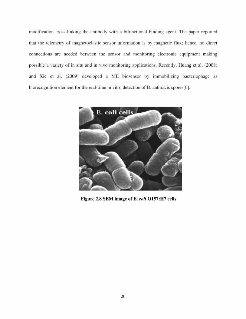
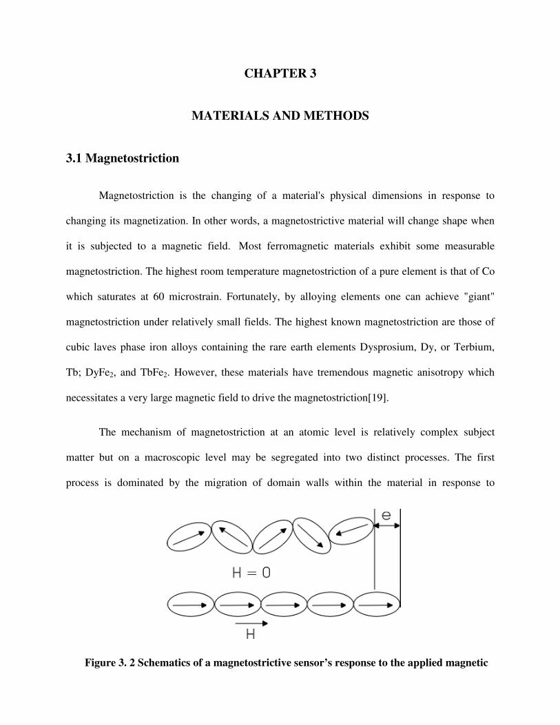
The mechanism of magnetostriction at an atomic level is relatively complex subject
matter but on a macroscopic level may be segregated into two distinct processes. The first
process is dominated by the migration of domain walls within the material in response to
Figure 3. 2 Schematics of a magnetostrictive sensor’s response to the applied magnetic
22
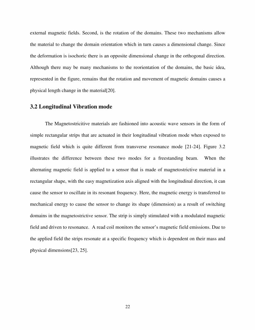
external magnetic fields. Second, is the rotation of the domains. These two mechanisms allow
the material to change the domain orientation which in turn causes a dimensional change. Since
the deformation is isochoric there is an opposite dimensional change in the orthogonal direction.
Although there may be many mechanisms to the reorientation of the domains, the basic idea,
represented in the figure, remains that the rotation and movement of magnetic domains causes a
physical length change in the material[20].
3.2 Longitudinal Vibration mode
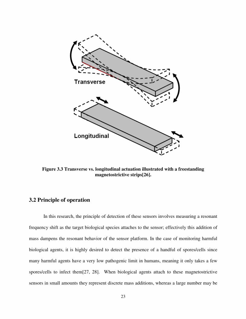
The Magnetostricitive materials are fashioned into acoustic wave sensors in the form of
simple rectangular strips that are actuated in their longitudinal vibration mode when exposed to
magnetic field which is quite different from transverse resonance mode [21-24]. Figure 3.2
illustrates the difference between these two modes for a freestanding beam. When the
alternating magnetic field is applied to a sensor that is made of magnetostrictive material in a
rectangular shape, with the easy magnetization axis aligned with the longitudinal direction, it can
cause the sensor to oscillate in its resonant frequency. Here, the magnetic energy is transferred to
mechanical energy to cause the sensor to change its shape (dimension) as a result of switching
domains in the magnetostrictive sensor. The strip is simply stimulated with a modulated magnetic
field and driven to resonance. A read coil monitors the sensor’s magnetic field emissions. Due to
the applied field the strips resonate at a specific frequency which is dependent on their mass and
physical dimensions[23, 25].
23
Figure 3.3 Transverse vs. longitudinal actuation illustrated with a freestanding
magnetostrictive strips[26].
3.2 Principle of operation
In this research, the principle of detection of these sensors involves measuring a resonant
frequency shift as the target biological species attaches to the sensor; effectively this addition of
mass dampens the resonant behavior of the sensor platform. In the case of monitoring harmful
biological agents, it is highly desired to detect the presence of a handful of spores/cells since
many harmful agents have a very low pathogenic limit in humans, meaning it only takes a few
spores/cells to infect them[27, 28]. When biological agents attach to these magnetostrictive
sensors in small amounts they represent discrete mass additions, whereas a large number may be
24
more analogous to mass evenly distributed on the strip. It is therefore highly desirable to better
understand how spore/cell attachment location influences the resonant frequency of these
magnetostrictive strips.
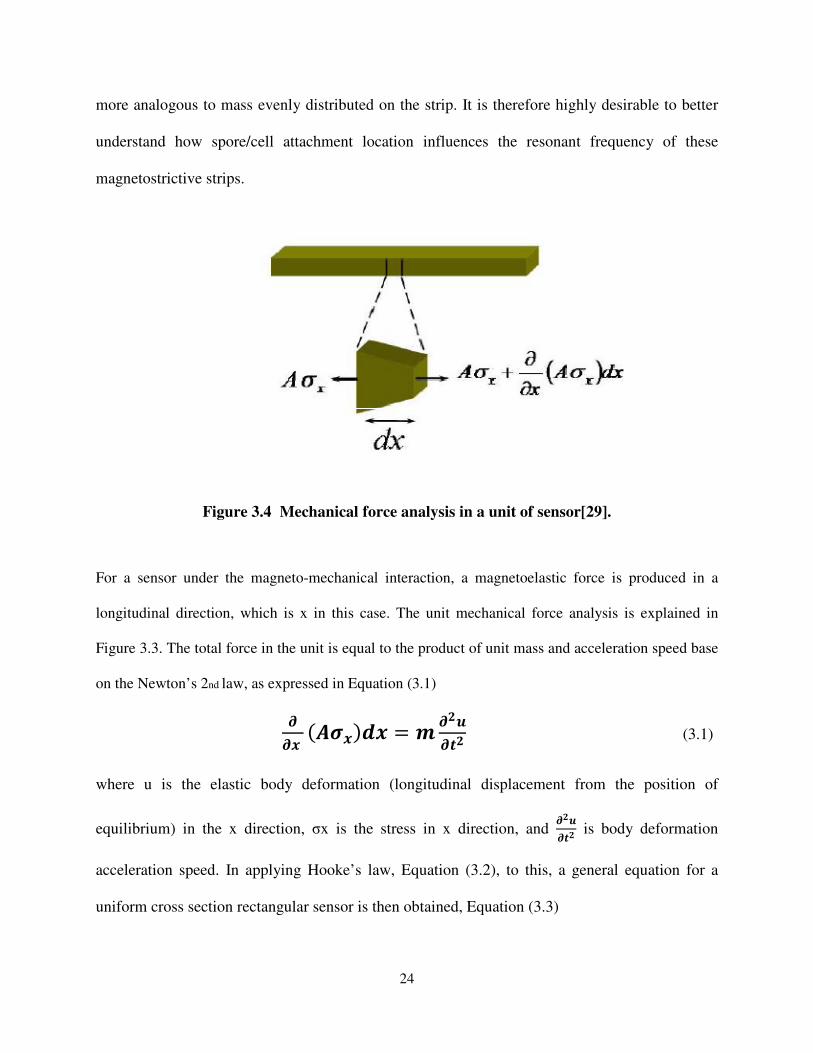
Figure 3.4 Mechanical force analysis in a unit of sensor[29].
For a sensor under the magneto-mechanical interaction, a magnetoelastic force is produced in a
longitudinal direction, which is x in this case. The unit mechanical force analysis is explained in
Figure 3.3. The total force in the unit is equal to the product of unit mass and acceleration speed base
on the Newton’s 2nd law, as expressed in Equation (3.1)
��� ������� = ���� � (3.1)
where u is the elastic body deformation (longitudinal displacement from the position of
equilibrium) in the x direction, σx is the stress in x direction, and ���� � is body deformation
acceleration speed. In applying Hooke’s law, Equation (3.2), to this, a general equation for a
uniform cross section rectangular sensor is then obtained, Equation (3.3)
25
�� = −��� = −� ���� (3.2)
���� � = �� ������ (3.3)
where u is the elastic body deformation (displacement) in x direction, and ���� , ������ are the strain
and strain rate, respectively. E and ρ correspondingly denote the Young’s modulus and density of
the sensor material. Young’s modulus E expressed here is dependent on the state of strain in the
structure. The elastic body deformation (displacement) u should be such a function of x and
(time) t as to satisfy the partial differential of Equation (3.3).
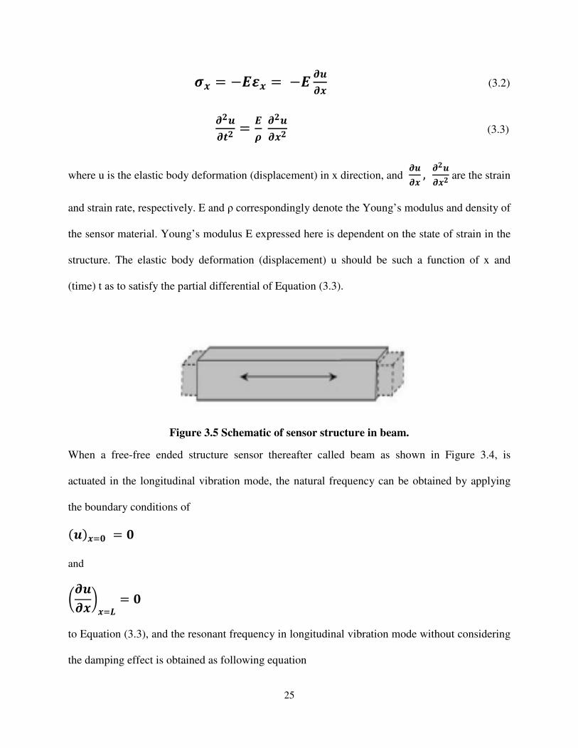
Figure 3.5 Schematic of sensor structure in beam.
When a free-free ended structure sensor thereafter called beam as shown in Figure 3.4, is
actuated in the longitudinal vibration mode, the natural frequency can be obtained by applying
the boundary conditions of
������ = �
and
��������� = �
to Equation (3.3), and the resonant frequency in longitudinal vibration mode without considering
the damping effect is obtained as following equation
26
� = ��� ��� (3.4)
Where n is integral, equals to 1,2,3….., for the first mode, n=1. L is the length of the sensor.
The basic sensor structure investigated was a freestanding beam with no fixed ends. The
resonance frequency of the first harmonic mode of such a structure can be described with the
damping effect is obtained with reference to Cai et. al [25]as,
� = ��� � ������� (3.5)
Where, L, E, and ρ are the length, Young’s modulus, and density of the sensor strip, respectively.
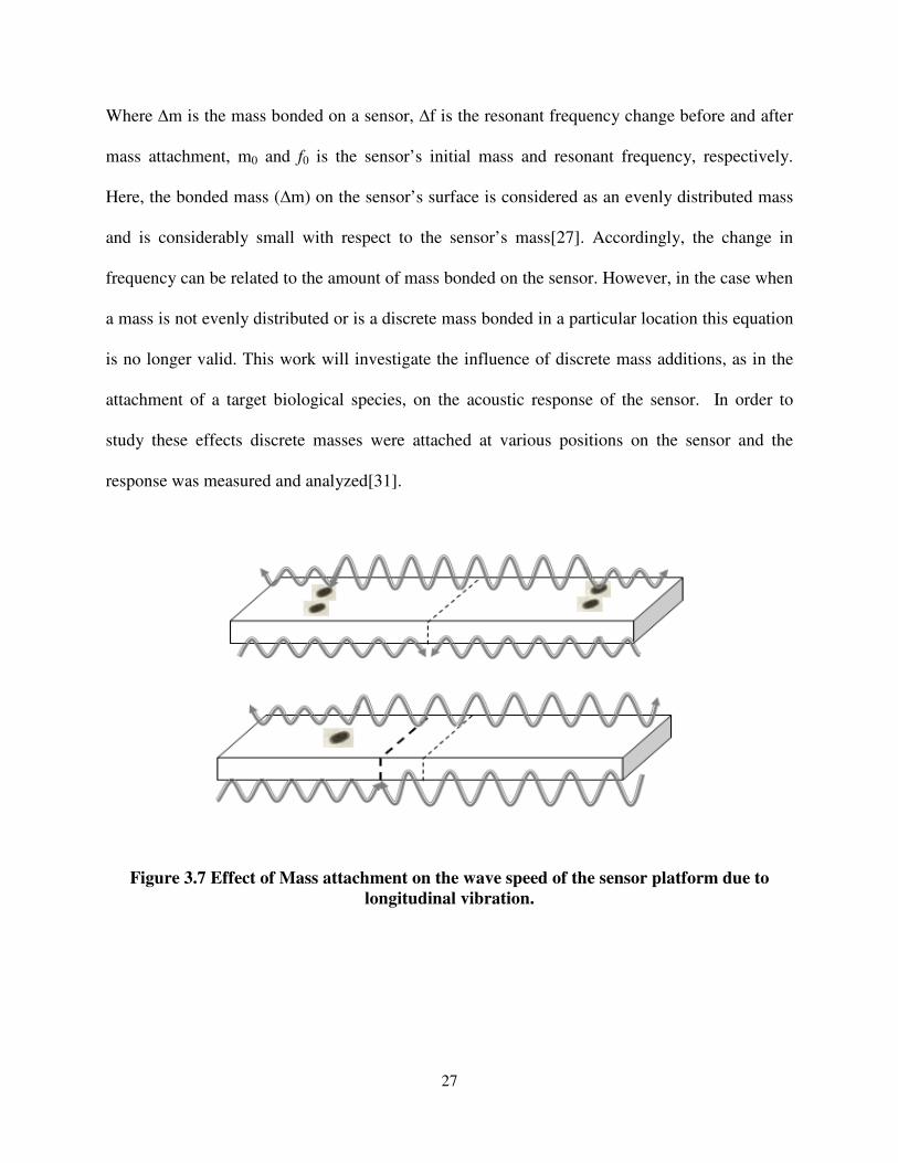
As these freestanding magnetostrictive strips are driven to their first harmonic mode, the entire
strip deforms in response to the field. The resulting deformation waves propagate through the
strip and reflect back from the free ends and cancel at the strip’s center, which is the zero nodal
position for a freestanding beam resonating in its first harmonic mode[30]. It should be noted
that positions further from the center node of the strip move further from the node during
deformation due to the accumulated deformations of all positions between it and the node. Thus,
the free ends move the furthest. When mass becomes attached to the sensor it effectively
dampens the speed of the deformation waves propagating in the strip, which reduces its resonant
frequency[14]. The frequency shift as a result of mass attachment for acoustic-based sensors
such as these is described the following equation,
∆� = − ��� ∆!"�# (3.6)
27
Where ∆m is the mass bonded on a sensor, ∆f is the resonant frequency change before and after
mass attachment, m0 and f0 is the sensor’s initial mass and resonant frequency, respectively.
Here, the bonded mass (∆m) on the sensor’s surface is considered as an evenly distributed mass
and is considerably small with respect to the sensor’s mass[27]. Accordingly, the change in
frequency can be related to the amount of mass bonded on the sensor. However, in the case when
a mass is not evenly distributed or is a discrete mass bonded in a particular location this equation
is no longer valid. This work will investigate the influence of discrete mass additions, as in the
attachment of a target biological species, on the acoustic response of the sensor. In order to
study these effects discrete masses were attached at various positions on the sensor and the
response was measured and analyzed[31].
Figure 3.7 Effect of Mass attachment on the wave speed of the sensor platform due to
longitudinal vibration.
28
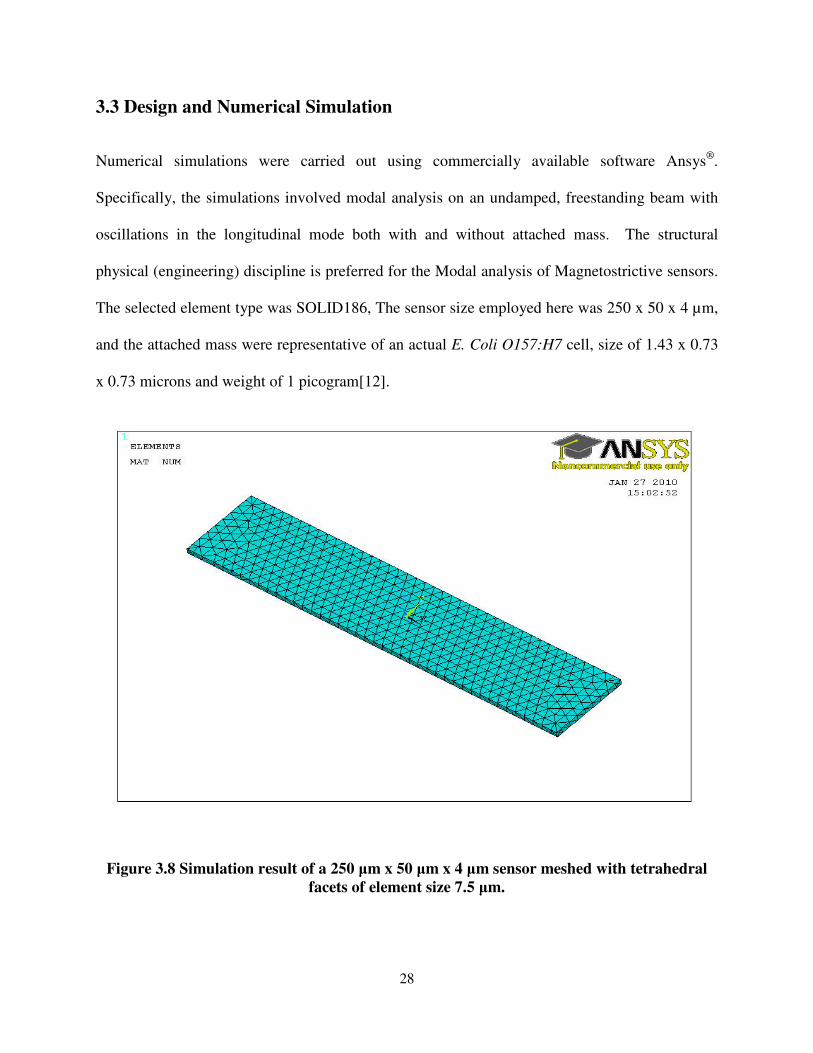
3.3 Design and Numerical Simulation
Numerical simulations were carried out using commercially available software Ansys®
.
Specifically, the simulations involved modal analysis on an undamped, freestanding beam with
oscillations in the longitudinal mode both with and without attached mass. The structural
physical (engineering) discipline is preferred for the Modal analysis of Magnetostrictive sensors.
The selected element type was SOLID186, The sensor size employed here was 250 x 50 x 4 µm,
and the attached mass were representative of an actual E. Coli O157:H7 cell, size of 1.43 x 0.73
x 0.73 microns and weight of 1 picogram[12].
Figure 3.8 Simulation result of a 250 µm x 50 µm x 4 µm sensor meshed with tetrahedral
facets of element size 7.5 µm.
29
The sensor platform was meshed with the element type tetrahedral facets of size 7.5 µm by
smartsizing option in the mesh tool as shown in Figure 3.6. The boundary conditions were set to
obtain longitudinal vibration mode of the sensor platform.
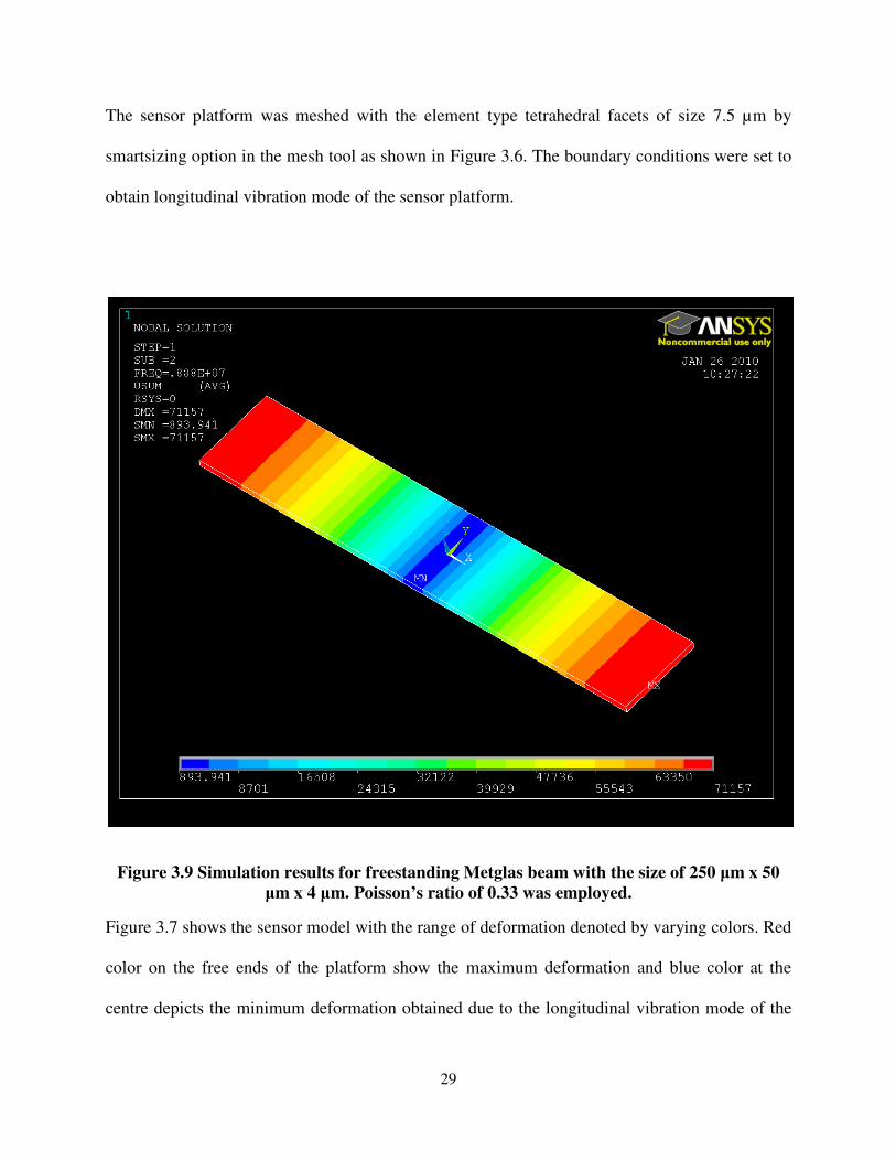
Figure 3.9 Simulation results for freestanding Metglas beam with the size of 250 µm x 50
µm x 4 µm. Poisson’s ratio of 0.33 was employed.
Figure 3.7 shows the sensor model with the range of deformation denoted by varying colors. Red
color on the free ends of the platform show the maximum deformation and blue color at the
centre depicts the minimum deformation obtained due to the longitudinal vibration mode of the
30
sensor platform. The simulation figure also provides the resonant frequency of 8.8753 MHz for
the default sensor dimension 250 x 50 x 4 µm used throughout our research work considered to
be fo. Prediction model was developed involving the factors influencing the resonance behavior
such as (a) Mass distribution, (b) Position of the mass distributed and (c) Physical dimension of
the sensor platform in compliance with the theoretical equations and simulation results. Mass of
E. coli cells were distributed as a single layer for uniform distribution. The later was glued to the
sensor platform and subjected to numerical simulation with the application of boundary
condition over the whole setup. The density of the layer was modified each time for different
amount of mass in uniform distribution case and the corresponding variation in frequency shift
was observed. In case of the non uniform distribution the layer was split and concentrated along
the free ends gradually moving towards the central nodal line and vice versa[23].
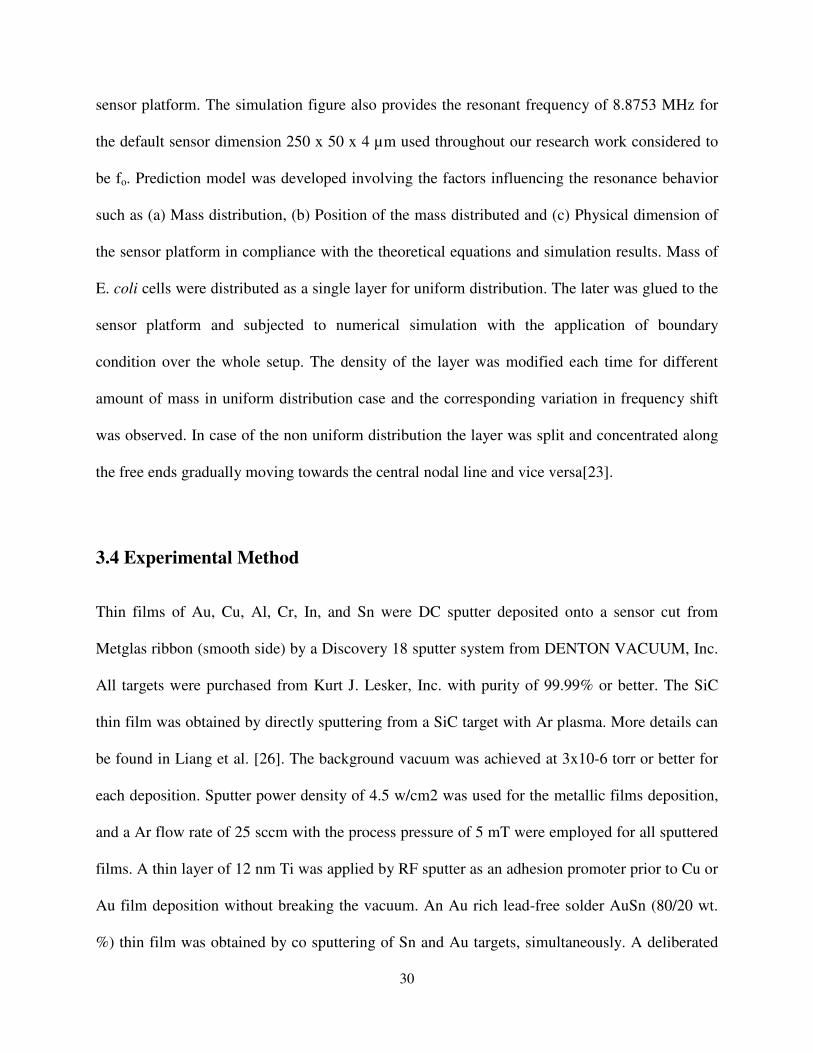
3.4 Experimental Method
Thin films of Au, Cu, Al, Cr, In, and Sn were DC sputter deposited onto a sensor cut from
Metglas ribbon (smooth side) by a Discovery 18 sputter system from DENTON VACUUM, Inc.
All targets were purchased from Kurt J. Lesker, Inc. with purity of 99.99% or better. The SiC
thin film was obtained by directly sputtering from a SiC target with Ar plasma. More details can
be found in Liang et al. [26]. The background vacuum was achieved at 3x10⁻⁶ torr or better for
each deposition. Sputter power density of 4.5 w/cm2 was used for the metallic films deposition,
and a Ar flow rate of 25 sccm with the process pressure of 5 mT were employed for all sputtered
films. A thin layer of 12 nm Ti was applied by RF sputter as an adhesion promoter prior to Cu or
Au film deposition without breaking the vacuum. An Au rich lead-free solder AuSn (80/20 wt.
%) thin film was obtained by co sputtering of Sn and Au targets, simultaneously. A deliberated
31
experiment was preformed to obtain the correct composition of AuSn (80/20) eutectic solder,
which was examined by EDX. All targets were sputter cleaned for 15 minutes with shutter
covered before deposition. Thin film thickness was controlled by sputtering time and measured
by a TENCOR alpha-step 200 profilometer from TENCOR Instruments, Inc. A Rigaku X-Ray
Vertical Diffractometer with Cu Kα radiation was employed to characterize the crystal structure
of these thin films, and the surface morphology of the film was characterized by using a JEOL
JSM 7000F field-emission SEM equipped with EDX capability. Metglas 2826 MB ribbon was
obtained from Metglas, Inc. and cut to sizes of 8 mmx1.6mm by a semiconductor ranked dicing
saw and cleaned with acetone, methanol, IPA(Isopropyl Alcohol), DI (deionized) water and
dried by nitrogen gas. The sensors were dehydrated in a convection oven at 120oC for 20 minutes
prior to use[29].
Figure 3.10 Procedural steps involved in the Microfabrication of Magnetostrictive strips
for the sensor platform.
32
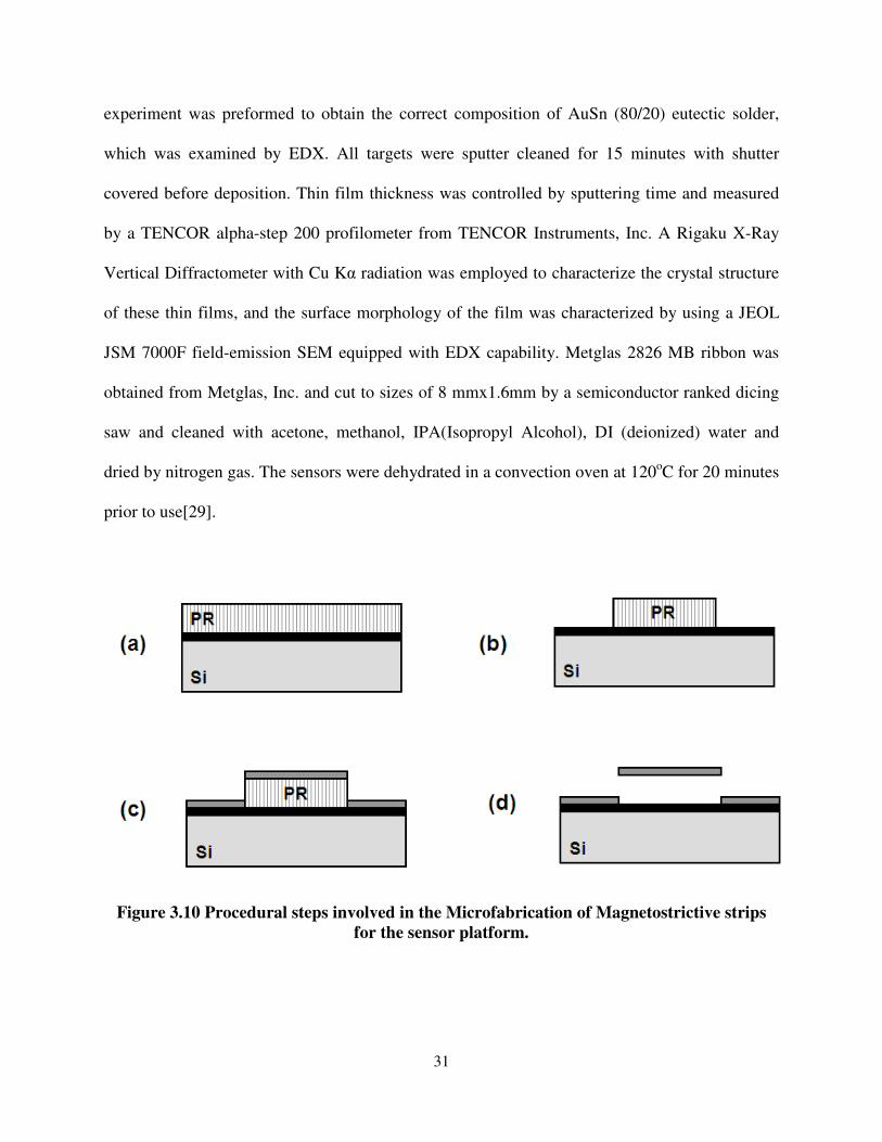
3.4.1 Glass beads attachement
Sensors with dimensions of 5 mm length and 1 mm width were cut from a 28 µm thick
commercially available Metglas 2826MB strip[15]. These specimens were prepared, by cleaning
and drying, using the identical procedures described by the authors elsewhere. Glass beads with a
diameter about 425 µm were employed to simulate the concentrated mass and were carefully
loaded on to the sensor surface at prescribed locations and secured with adhesive. The average
mass of a sensor and glass bead were 1066 µg and 181.5 µg, respectively.
Figure 3.11 SEM images showing glass beads attached to the sensor in various locations.
It should be noted that these experiments are aimed as assessing the position of the mass
concentrations and not focused on demonstrating minimum sensitivity. Thus, significantly sized
beads were employed as shown in Figure 3.9. The amount of glue employed to affix each bead
33
as well as its position were well controlled to minimize any errors. After a glass bead was loaded
on the sensor surface, it was immobilized by drying at room temperature for at least two hours.
The resonant frequency of the sensor was measured before and after attachment of the glass bead
in a manner identical to which is discussed in previous work by the authors [5, 32-34].
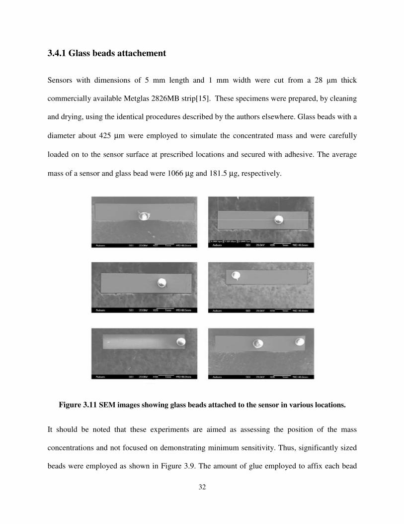
3.4.2 Detection Setup
The test setup consists of three key units, a HP8751A network analyzer (a), a custom made read
coil that serves as a A/C magnetic field generator and sensor’s signal pick up (b), and a
permanent magnetic bar that serve as a magnetic bias field (c), as shown in Figure 3.4. Note that
the read coil is directly connected to port 1 of the network analyzer and both the read coil and
magnetic bar are not in scale. They are enlarged for better observation.
Figure 3.12 Resonant frequency detection setup containing Actuation/read coil, and magnetic
bar
34
The characteristics of a magnetostrictive sensor can be characterized through this set up. The
basics can be described as follows: when the analyzer sends a RF swept signal (exciting signal)
or power, through the coil, which generates an A/C magnetic field in the coil, a magnetostrictive
sensor inside the coil will alternatively change its shape or vibration as a result of response to
this A/C magnetic field. Such change in shape of the sensor will produce a second; an alternative
magnetic field that will interacts with the read coil (also called pick up) to generate a second, an
alternatively signal at the same frequency as the applied RF signal. When the frequency of the
applied RF swept signal reaches the resonant frequency of the magnetostrictive strips, oscillation
occurs, and the strips are deformed, therefore, reaching its maximum. Consequently, this is the
largest interaction between the magnetostrictive strips and the pick-up coil. This largest
interaction results in the largest power change in the device under test (DUT) and network,
which is analyzed by the network analyzer through measuring either the transmitted or the
reflected signal[29].
35
CHAPTER 4
RESULTS AND DISCUSSION
4.1 Distribution of Mass
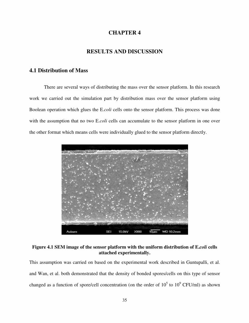
There are several ways of distributing the mass over the sensor platform. In this research
work we carried out the simulation part by distribution mass over the sensor platform using
Boolean operation which glues the E.coli cells onto the sensor platform. This process was done
with the assumption that no two E.coli cells can accumulate to the sensor platform in one over
the other format which means cells were individually glued to the sensor platform directly.
Figure 4.1 SEM image of the sensor platform with the uniform distribution of E.coli cells
attached experimentally.
This assumption was carried on based on the experimental work described in Guntupalli, et al.
and Wan, et al. both demonstrated that the density of bonded spores/cells on this type of sensor
changed as a function of spore/cell concentration (on the order of 105 to 10
9 CFU/ml) as shown
36
in Figure 4.1. Other observations in these papers included that the uniformity of bonded
spores/cells decreased when spore/cell concentration decreased and that there was a significant
discrepancy between the number of bonded spores/cells experimentally observed and
theoretically predicted on the surface. This is because the bacteriophage they use to immobilize
the sensor platform can hold one cell per phage and that would limit the number of cells attached
to the sensor platform.
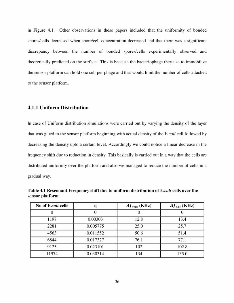
4.1.1 Uniform Distribution
In case of Uniform distribution simulations were carried out by varying the density of the layer
that was glued to the sensor platform beginning with actual density of the E.coli cell followed by
decreasing the density upto a certain level. Accordingly we could notice a linear decrease in the
frequency shift due to reduction in density. This basically is carried out in a way that the cells are
distributed uniformly over the platform and also we managed to reduce the number of cells in a
gradual way.
Table 4.1 Reseonant Frequency shift due to uniform distribution of E.coli cells over the
sensor platform
No of E.coli cells η $�!% (KHz) $�&'( �KHz)
0 0 0 0
1197 0.00303 12.8 13.4
2281 0.005775 25.0 25.7
4563 0.011552 50.6 51.4
6844 0.017327 76.1 77.1
9125 0.023101 102 102.8
11974 0.030314 134 135.0
Considering the upper surface of the sensor platform
that the maximum possible number of cells were 12000. The cells co
and we can see the corresponding decrease in the frequency shift. Figure 4.
frequency shift of the sensor
represents the calculated value for the corresponding numb
The square dots were the simulated result values obtained following the boundary conditions and
other required specifications for the modal analysis of the sensor in Ansys.
Figure 4.2 Resonant Frequency Shift due to uniform distribution of E.
37
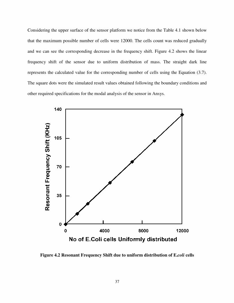
Considering the upper surface of the sensor platform we notice from the Table
that the maximum possible number of cells were 12000. The cells count was reduced gradually
and we can see the corresponding decrease in the frequency shift. Figure 4.2
due to uniform distribution of mass. The straight dark line
represents the calculated value for the corresponding number of cells using the Equation (3.7)
The square dots were the simulated result values obtained following the boundary conditions and
er required specifications for the modal analysis of the sensor in Ansys.
Resonant Frequency Shift due to uniform distribution of E.
4.1 shown below
unt was reduced gradually
shows the linear
to uniform distribution of mass. The straight dark line
er of cells using the Equation (3.7).
The square dots were the simulated result values obtained following the boundary conditions and
Resonant Frequency Shift due to uniform distribution of E.coli cells
38
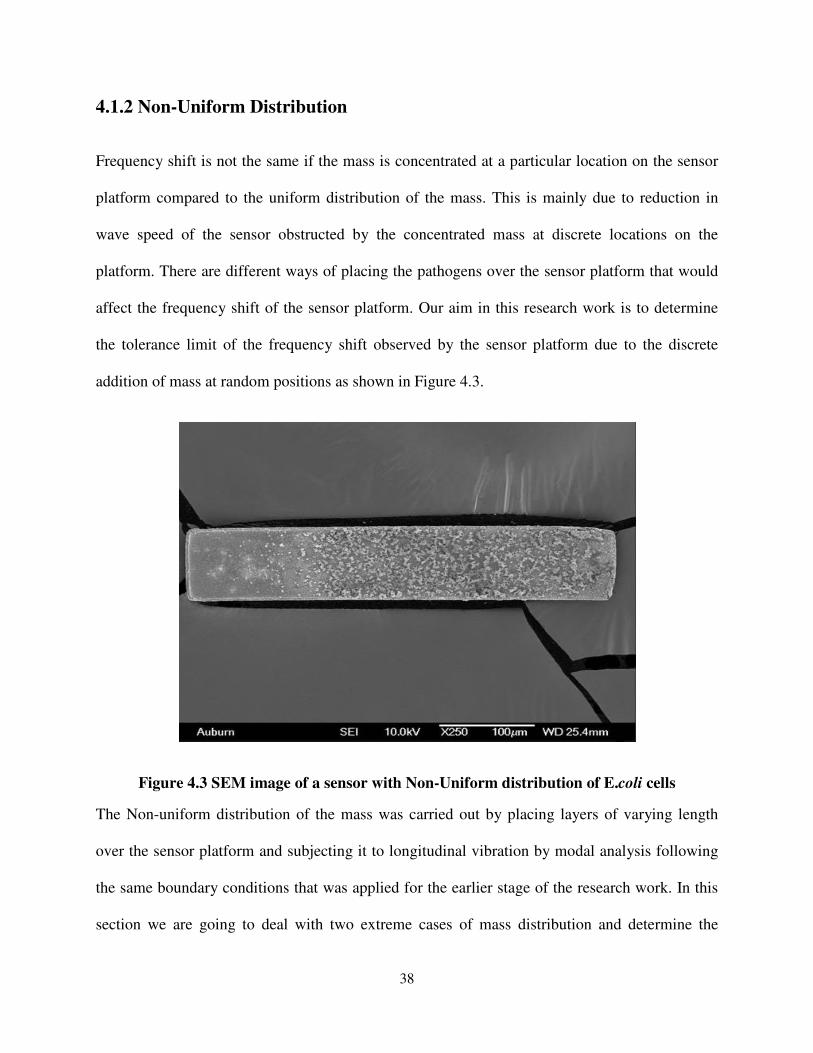
4.1.2 Non-Uniform Distribution
Frequency shift is not the same if the mass is concentrated at a particular location on the sensor
platform compared to the uniform distribution of the mass. This is mainly due to reduction in
wave speed of the sensor obstructed by the concentrated mass at discrete locations on the
platform. There are different ways of placing the pathogens over the sensor platform that would
affect the frequency shift of the sensor platform. Our aim in this research work is to determine
the tolerance limit of the frequency shift observed by the sensor platform due to the discrete
addition of mass at random positions as shown in Figure 4.3.
Figure 4.3 SEM image of a sensor with Non-Uniform distribution of E.coli cells
The Non-uniform distribution of the mass was carried out by placing layers of varying length
over the sensor platform and subjecting it to longitudinal vibration by modal analysis following
the same boundary conditions that was applied for the earlier stage of the research work. In this
section we are going to deal with two extreme cases of mass distribution and determine the
39
tolerance limit with the help of the simulation results. To uphold the simulation results we have
theoretical derivations and corresponding mathematical calculations.
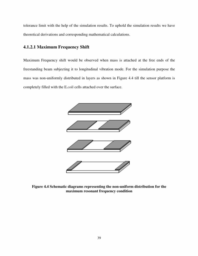
4.1.2.1 Maximum Frequency Shift
Maximum Frequency shift would be observed when mass is attached at the free ends of the
freestanding beam subjecting it to longitudinal vibration mode. For the simulation purpose the
mass was non-uniformly distributed in layers as shown in Figure 4.4 till the sensor platform is
completely filled with the E.coli cells attached over the surface.
Figure 4.4 Schematic diagrams representing the non-uniform distribution for the
maximum resonant frequency condition
40
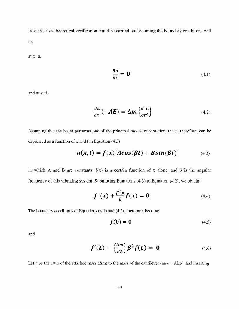
In such cases theoretical verification could be carried out assuming the boundary conditions will
be
at x=0,
���� = � (4.1)
and at x=L,
���� �−��� = ∆ ���� � # (4.2)
Assuming that the beam performs one of the principal modes of vibration, the u, therefore, can be
expressed as a function of x and t in Equation (4.3)
���, � = ����)�&�!�* � + ,!%��* �- (4.3)
in which A and B are constants, f(x) is a certain function of x alone, and β is the angular
frequency of this vibrating system. Submitting Equations (4.3) to Equation (4.2), we obtain:
�"��� + *��� ���� = � (4.4)
The boundary conditions of Equations (4.1) and (4.2), therefore, become
���� = � (4.5)
and
�/��� − 0��# *����� = � (4.6)
Let η be the ratio of the attached mass (∆m) to the mass of the cantilever (msen = ALρ), and inserting

41
1 = ∆!"� = ∆���
into Equation (4.6), we have
�/��� − 1� �*�� # ���� = �
(4.7)
Thus the standard solution for Equation (4.4) is
���� = 2&�! �*��� �� + 3!%� �*��� �� (4.8) To satisfy the boundary condition: f (0) = 0, C must vanish and β must be real. Equation (4.8)
therefore becomes
���� = 3!%� �*��� �� (4.9)
To meet the boundary condition of Equation (4.7), Equation (4.8) becomes
&�! �*����� = 1 �*����� !%� �*����� (4.10)
1 4�*���5 = − '� 4�*���5
Where
6 = *���
1�6�� = −789 �6�� (4.11)
42
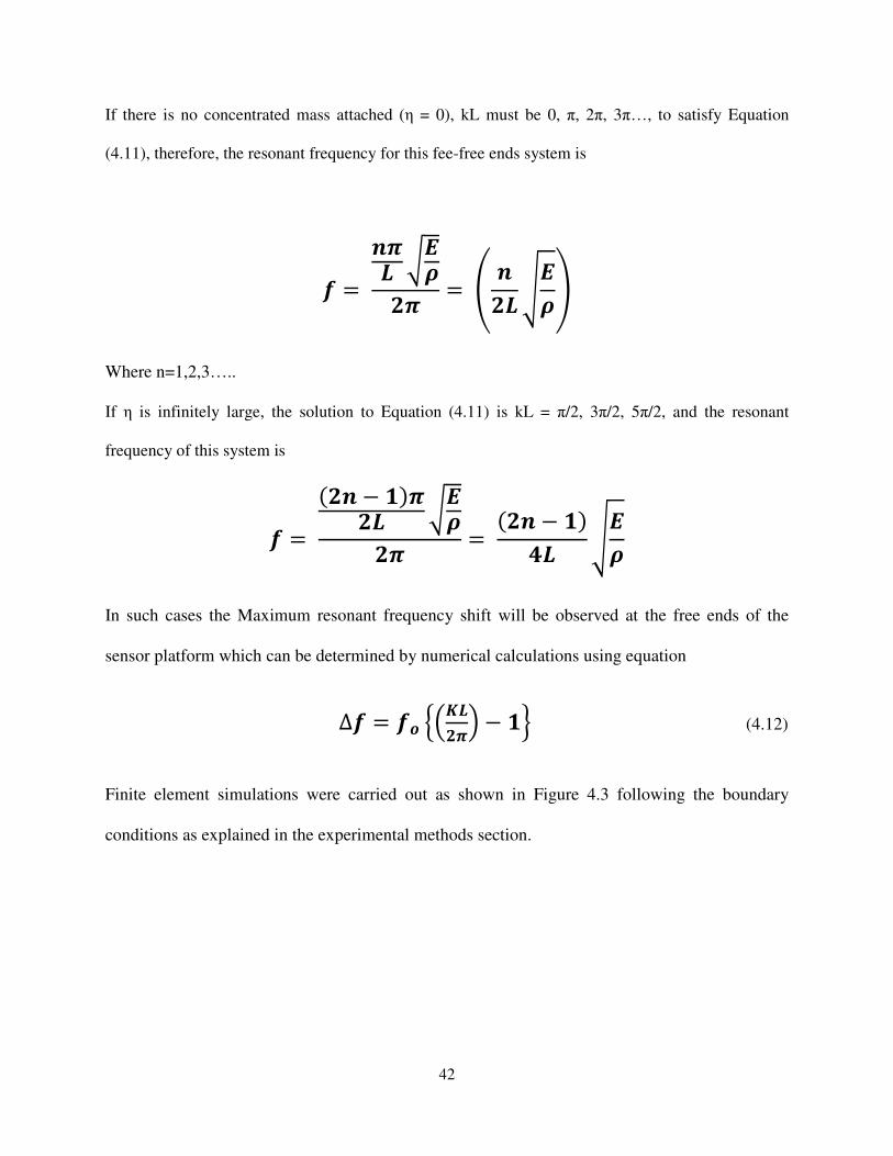
If there is no concentrated mass attached (η = 0), kL must be 0, π, 2π, 3π…, to satisfy Equation
(4.11), therefore, the resonant frequency for this fee-free ends system is
� = �:� ����: = ; ��� <��= Where n=1,2,3…..
If η is infinitely large, the solution to Equation (4.11) is kL = π/2, 3π/2, 5π/2, and the resonant
frequency of this system is
� = ��� − ��:�� ����: = ��� − ��>� <��
In such cases the Maximum resonant frequency shift will be observed at the free ends of the
sensor platform which can be determined by numerical calculations using equation
∆� = �� ?6��:@ − �# (4.12)
Finite element simulations were carried out as shown in Figure 4.3 following the boundary
conditions as explained in the experimental methods section.
43
Table 4.2 Calculated values of η and KL with the corresponding resonant frequency shift
values determined using the Equation (4.12) and (3.6)
η 0 0.0005 0.005 0.01 0.05 0.5 1 ∞
KL π 3.1400225 3.125965 3.110498 2.99304 2.28893 2.02876 π/2
ABCDE
(KHz)
0 4.452 44.312 88.168 421.205 2408.853 3155.378 4437.650
ABFGH �IJK�
0 2.226 22.269 44.539 222.695 2218.825 4437.650 ∞
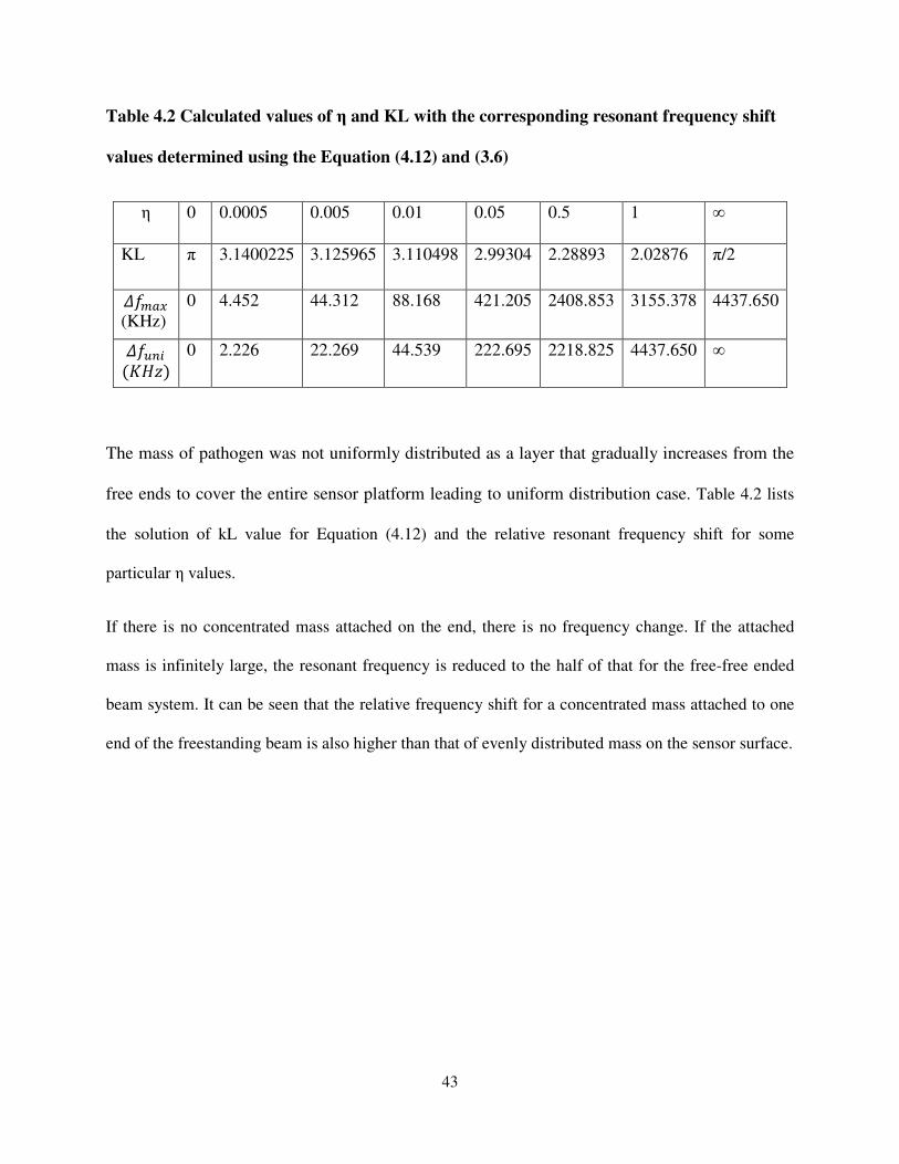
The mass of pathogen was not uniformly distributed as a layer that gradually increases from the
free ends to cover the entire sensor platform leading to uniform distribution case. Table 4.2 lists
the solution of kL value for Equation (4.12) and the relative resonant frequency shift for some
particular η values.
If there is no concentrated mass attached on the end, there is no frequency change. If the attached
mass is infinitely large, the resonant frequency is reduced to the half of that for the free-free ended
beam system. It can be seen that the relative frequency shift for a concentrated mass attached to one
end of the freestanding beam is also higher than that of evenly distributed mass on the sensor surface.
44
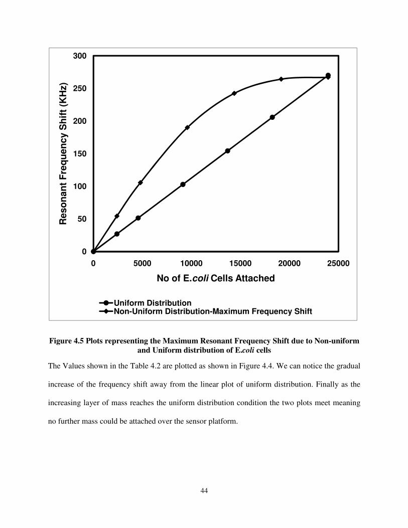
Figure 4.5 Plots representing the Maximum Resonant Frequency Shift due to Non-uniform
and Uniform distribution of E.coli cells
The Values shown in the Table 4.2 are plotted as shown in Figure 4.4. We can notice the gradual
increase of the frequency shift away from the linear plot of uniform distribution. Finally as the
increasing layer of mass reaches the uniform distribution condition the two plots meet meaning
no further mass could be attached over the sensor platform.
0
50
100
150
200
250
300
0 5000 10000 15000 20000 25000
Reso
nan
t F
req
uen
cy S
hif
t (K
Hz)
No of E.coli Cells Attached
Uniform DistributionNon-Uniform Distribution-Maximum Frequency Shift
45
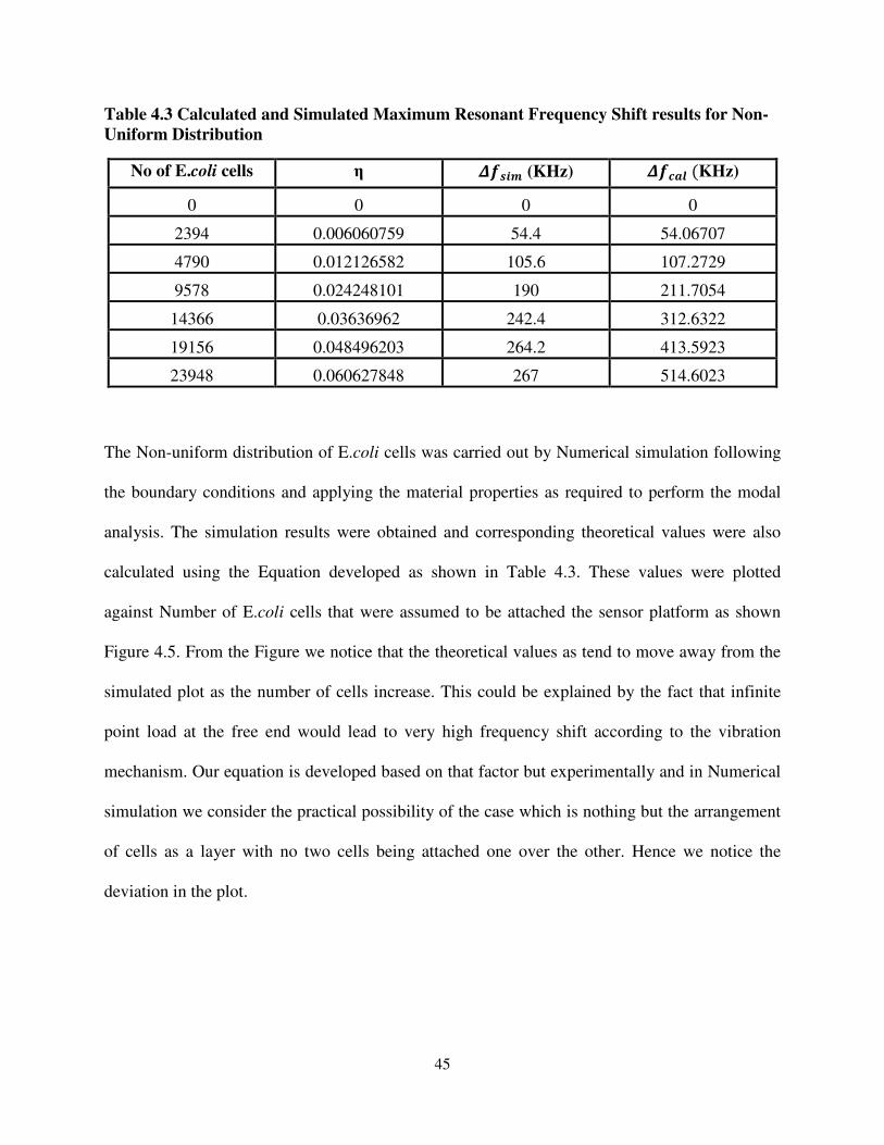
Table 4.3 Calculated and Simulated Maximum Resonant Frequency Shift results for Non-
Uniform Distribution
No of E.coli cells η $�!% (KHz) $�&'( �KHz)
0 0 0 0
2394 0.006060759 54.4 54.06707
4790 0.012126582 105.6 107.2729
9578 0.024248101 190 211.7054
14366 0.03636962 242.4 312.6322
19156 0.048496203 264.2 413.5923
23948 0.060627848 267 514.6023
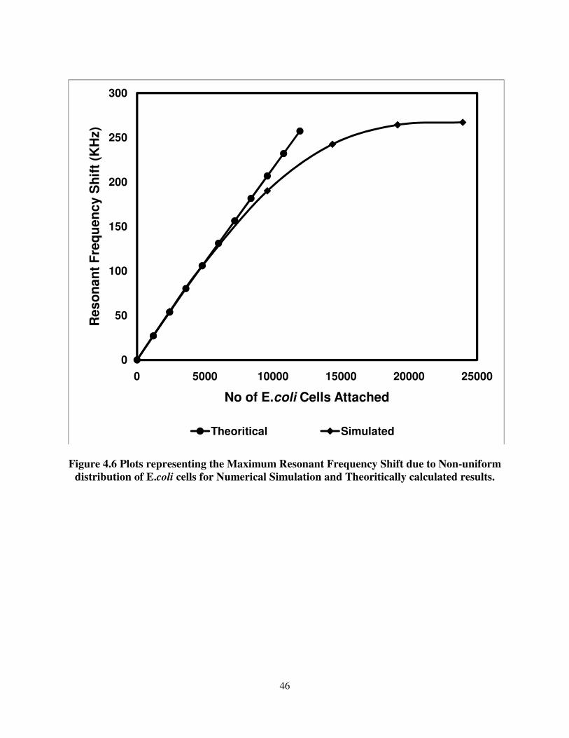
The Non-uniform distribution of E.coli cells was carried out by Numerical simulation following
the boundary conditions and applying the material properties as required to perform the modal
analysis. The simulation results were obtained and corresponding theoretical values were also
calculated using the Equation developed as shown in Table 4.3. These values were plotted
against Number of E.coli cells that were assumed to be attached the sensor platform as shown
Figure 4.5. From the Figure we notice that the theoretical values as tend to move away from the
simulated plot as the number of cells increase. This could be explained by the fact that infinite
point load at the free end would lead to very high frequency shift according to the vibration
mechanism. Our equation is developed based on that factor but experimentally and in Numerical
simulation we consider the practical possibility of the case which is nothing but the arrangement
of cells as a layer with no two cells being attached one over the other. Hence we notice the
deviation in the plot.
46
Figure 4.6 Plots representing the Maximum Resonant Frequency Shift due to Non-uniform
distribution of E.coli cells for Numerical Simulation and Theoritically calculated results.
0
50
100
150
200
250
300
0 5000 10000 15000 20000 25000
Reso
nan
t F
req
uen
cy S
hif
t (K
Hz)
No of E.coli Cells Attached
Theoritical Simulated
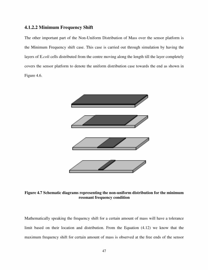
4.1.2.2 Minimum Frequency
The other important part of the Non
the Minimum Frequency shift case. This case is carried out through simulation by having the
layers of E.coli cells distributed from the centre moving along
covers the sensor platform to denote the uniform distribution case towards the end as shown in
Figure 4.6.
Figure 4.7 Schematic diagrams representing the non
Mathematically speaking the frequency shift for a certain amount of mass will have a tolerance
limit based on their location and distribution. From the
maximum frequency shift for certain amount of mass is observed
47
4.1.2.2 Minimum Frequency Shift
The other important part of the Non-Uniform Distribution of Mass over the sensor platform is
the Minimum Frequency shift case. This case is carried out through simulation by having the
cells distributed from the centre moving along the length till the layer completely
covers the sensor platform to denote the uniform distribution case towards the end as shown in
Schematic diagrams representing the non-uniform distribution for the minimum
resonant frequency condition
Mathematically speaking the frequency shift for a certain amount of mass will have a tolerance
limit based on their location and distribution. From the Equation (4.12) we know that the
maximum frequency shift for certain amount of mass is observed at the free ends of the sensor
Uniform Distribution of Mass over the sensor platform is
the Minimum Frequency shift case. This case is carried out through simulation by having the
the length till the layer completely
covers the sensor platform to denote the uniform distribution case towards the end as shown in
uniform distribution for the minimum
Mathematically speaking the frequency shift for a certain amount of mass will have a tolerance
we know that the
at the free ends of the sensor
48
platform. This eventually explains the fact that the minimum frequency shift for the same
amount of mass would be observed when concentrated at the centre. When mass is distributed
close to the nodal point since the deformation experienced is relatively lower compared to the
free ends , we observe minimum frequency shift close the centerline of the sensor platform.
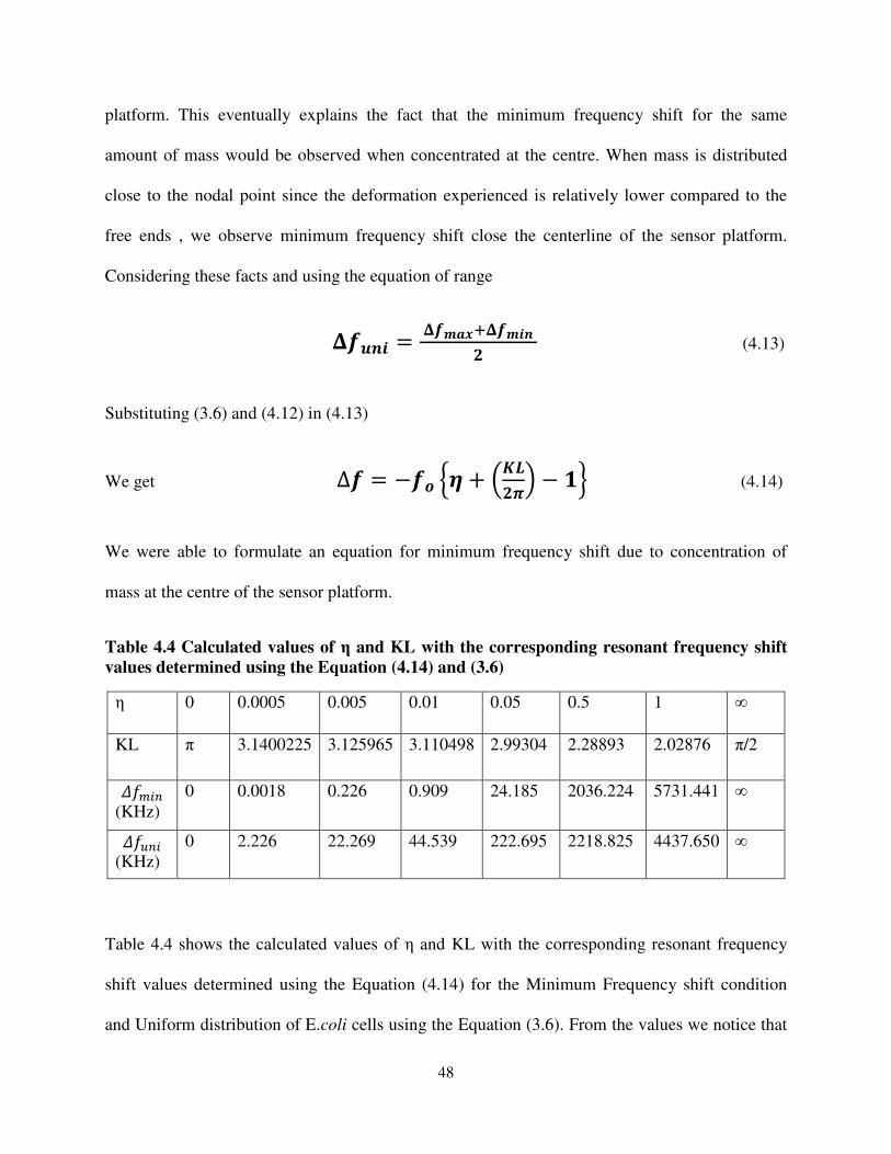
Considering these facts and using the equation of range
0���% = 0�'�L0�%� � (4.13)
Substituting (3.6) and (4.12) in (4.13)
We get ∆� = −�� 1 + ?6��:@ − �# (4.14)
We were able to formulate an equation for minimum frequency shift due to concentration of
mass at the centre of the sensor platform.
Table 4.4 Calculated values of η and KL with the corresponding resonant frequency shift
values determined using the Equation (4.14) and (3.6)
η 0 0.0005 0.005 0.01 0.05 0.5 1 ∞
KL π 3.1400225 3.125965 3.110498 2.99304 2.28893 2.02876 π/2
ABCHG
(KHz)
0 0.0018 0.226 0.909 24.185 2036.224 5731.441 ∞
ABFGH (KHz)
0 2.226 22.269 44.539 222.695 2218.825 4437.650 ∞
Table 4.4 shows the calculated values of η and KL with the corresponding resonant frequency
shift values determined using the Equation (4.14) for the Minimum Frequency shift condition
and Uniform distribution of E.coli cells using the Equation (3.6). From the values we notice that
49
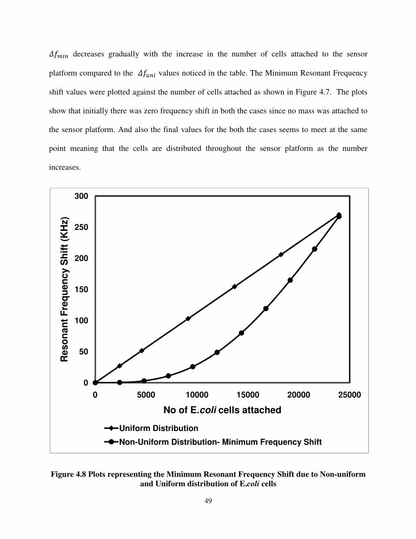
ABCHG decreases gradually with the increase in the number of cells attached to the sensor
platform compared to the ABFGH values noticed in the table. The Minimum Resonant Frequency
shift values were plotted against the number of cells attached as shown in Figure 4.7. The plots
show that initially there was zero frequency shift in both the cases since no mass was attached to
the sensor platform. And also the final values for the both the cases seems to meet at the same
point meaning that the cells are distributed throughout the sensor platform as the number
increases.
Figure 4.8 Plots representing the Minimum Resonant Frequency Shift due to Non-uniform
and Uniform distribution of E.coli cells
0
50
100
150
200
250
300
0 5000 10000 15000 20000 25000
Reso
nan
t F
req
uen
cy S
hif
t (K
Hz)
No of E.coli cells attached
Uniform Distribution
Non-Uniform Distribution- Minimum Frequency Shift
50
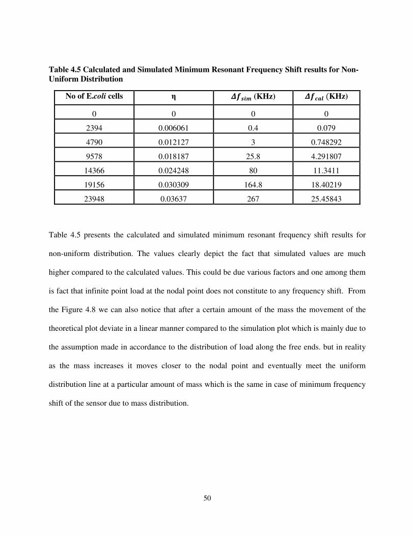
Table 4.5 Calculated and Simulated Minimum Resonant Frequency Shift results for Non-
Uniform Distribution
No of E.coli cells η $�!% (KHz) $�&'( �KHz)
0 0 0 0
2394 0.006061 0.4 0.079
4790 0.012127 3 0.748292
9578 0.018187 25.8 4.291807
14366 0.024248 80 11.3411
19156 0.030309 164.8 18.40219
23948 0.03637 267 25.45843
Table 4.5 presents the calculated and simulated minimum resonant frequency shift results for
non-uniform distribution. The values clearly depict the fact that simulated values are much
higher compared to the calculated values. This could be due various factors and one among them
is fact that infinite point load at the nodal point does not constitute to any frequency shift. From
the Figure 4.8 we can also notice that after a certain amount of the mass the movement of the
theoretical plot deviate in a linear manner compared to the simulation plot which is mainly due to
the assumption made in accordance to the distribution of load along the free ends. but in reality
as the mass increases it moves closer to the nodal point and eventually meet the uniform
distribution line at a particular amount of mass which is the same in case of minimum frequency
shift of the sensor due to mass distribution.
51
Figure 4.9 Plots representing the Minimum Resonant Frequency Shift due to Non-uniform
distribution of E.coli cells for Numerical Simulation and Theoritically calculated results.
In the previous two sections we discussed the major factor that affects the Resonant Frequency
of the sensor which was focused in detail for the detection of biological specimens. The
Equations were formulated to verify the results obtained by numerical simulations. Figure 4.9
provides the complete tolerance limit of the possible frequency shift that could be expected from
the sensor when subjected to longitudinal vibration mode due to the distribution of mass. The
0
50
100
150
200
250
300
0 5000 10000 15000 20000 25000
Reso
nan
t F
req
uen
cy S
hif
t (K
Hz)
No of E.coli Cells Attached
Theoritical Simulated
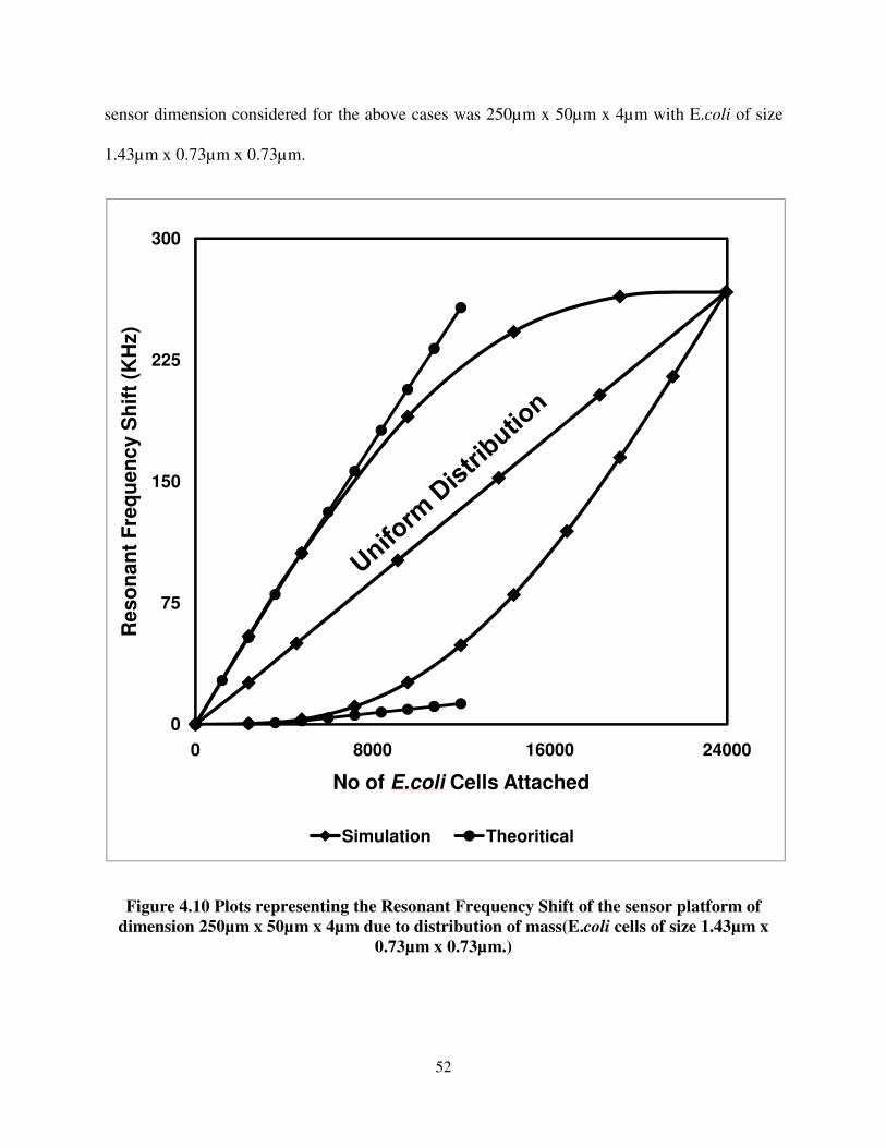
52
sensor dimension considered for the above cases was 250µm x 50µm x 4µm with E.coli of size
1.43µm x 0.73µm x 0.73µm.
Figure 4.10 Plots representing the Resonant Frequency Shift of the sensor platform of
dimension 250µm x 50µm x 4µm due to distribution of mass(E.coli cells of size 1.43µm x
0.73µm x 0.73µm.)
0
75
150
225
300
0 8000 16000 24000
Reso
nan
t F
req
uen
cy S
hif
t (K
Hz)
No of E.coli Cells Attached
Simulation Theoritical
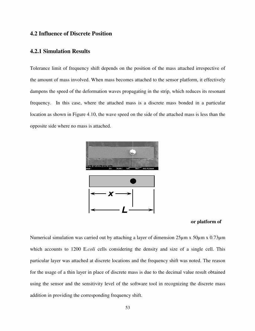
4.2 Influence of Discrete Position
4.2.1 Simulation Results
Tolerance limit of frequency shift depends on the position of
the amount of mass involved. When mass becomes attached to the sensor platform, it effectively
dampens the speed of the deformation waves propagating in the strip, which reduces its resonant
frequency. In this case, where
location as shown in Figure 4.10
opposite side where no mass is attached.
Numerical simulation was carried out by attach
which accounts to 1200 E.coli
particular layer was attached at discrete locations and the frequency shift was noted. The reason
for the usage of a thin layer in place of discrete mass is due to the decimal value result obtained
using the sensor and the sensitivity level of the software tool in recognizing the discrete mass
addition in providing the corresponding frequency shift.
Figure 4.11 Addition of concentrated mass
53
4.2 Influence of Discrete Position
Tolerance limit of frequency shift depends on the position of the mass attached irrespective of
When mass becomes attached to the sensor platform, it effectively
dampens the speed of the deformation waves propagating in the strip, which reduces its resonant
frequency. In this case, where the attached mass is a discrete mass bonded in a particular
as shown in Figure 4.10, the wave speed on the side of the attached mass is less than the
opposite side where no mass is attached.
Numerical simulation was carried out by attaching a layer of dimension 25µm x 50µm x
cells considering the density and size of a single cell. This
particular layer was attached at discrete locations and the frequency shift was noted. The reason
hin layer in place of discrete mass is due to the decimal value result obtained
using the sensor and the sensitivity level of the software tool in recognizing the discrete mass
addition in providing the corresponding frequency shift.
Addition of concentrated mass at discrete location x on the sensor platform of
length L
the mass attached irrespective of
When mass becomes attached to the sensor platform, it effectively
dampens the speed of the deformation waves propagating in the strip, which reduces its resonant
mass is a discrete mass bonded in a particular
, the wave speed on the side of the attached mass is less than the
ing a layer of dimension 25µm x 50µm x 0.73µm
cells considering the density and size of a single cell. This
particular layer was attached at discrete locations and the frequency shift was noted. The reason
hin layer in place of discrete mass is due to the decimal value result obtained
using the sensor and the sensitivity level of the software tool in recognizing the discrete mass
at discrete location x on the sensor platform of
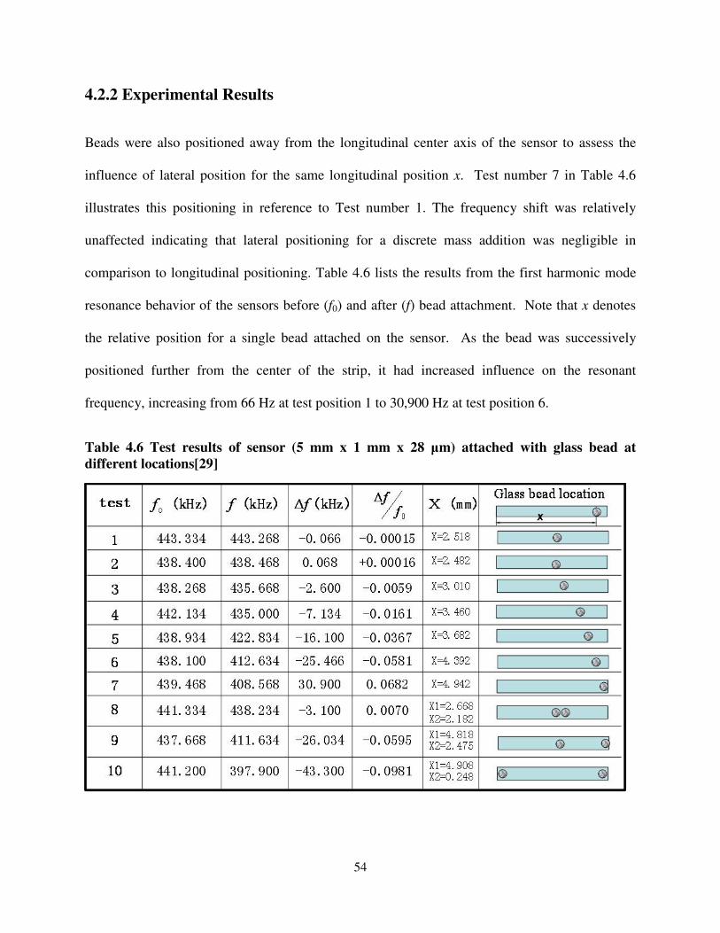
54
4.2.2 Experimental Results
Beads were also positioned away from the longitudinal center axis of the sensor to assess the
influence of lateral position for the same longitudinal position x. Test number 7 in Table 4.6
illustrates this positioning in reference to Test number 1. The frequency shift was relatively
unaffected indicating that lateral positioning for a discrete mass addition was negligible in
comparison to longitudinal positioning. Table 4.6 lists the results from the first harmonic mode
resonance behavior of the sensors before (f0) and after (f) bead attachment. Note that x denotes
the relative position for a single bead attached on the sensor. As the bead was successively
positioned further from the center of the strip, it had increased influence on the resonant
frequency, increasing from 66 Hz at test position 1 to 30,900 Hz at test position 6.
Table 4.6 Test results of sensor (5 mm x 1 mm x 28 µm) attached with glass bead at
different locations[29]
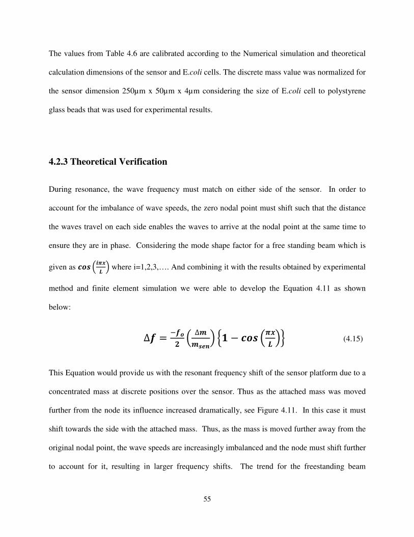
55
The values from Table 4.6 are calibrated according to the Numerical simulation and theoretical
calculation dimensions of the sensor and E.coli cells. The discrete mass value was normalized for
the sensor dimension 250µm x 50µm x 4µm considering the size of E.coli cell to polystyrene
glass beads that was used for experimental results.
4.2.3 Theoretical Verification
During resonance, the wave frequency must match on either side of the sensor. In order to
account for the imbalance of wave speeds, the zero nodal point must shift such that the distance
the waves travel on each side enables the waves to arrive at the nodal point at the same time to
ensure they are in phase. Considering the mode shape factor for a free standing beam which is
given as &�! ?%:�� @ where i=1,2,3,…. And combining it with the results obtained by experimental
method and finite element simulation we were able to develop the Equation 4.11 as shown
below:
∆� = ���� ? ∆!"�@ � − &�! ?:�� @# (4.15)
This Equation would provide us with the resonant frequency shift of the sensor platform due to a
concentrated mass at discrete positions over the sensor. Thus as the attached mass was moved
further from the node its influence increased dramatically, see Figure 4.11. In this case it must
shift towards the side with the attached mass. Thus, as the mass is moved further away from the
original nodal point, the wave speeds are increasingly imbalanced and the node must shift further
to account for it, resulting in larger frequency shifts. The trend for the freestanding beam
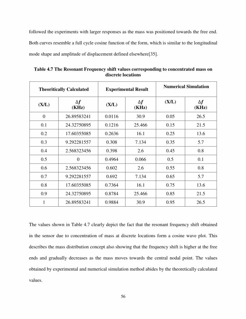
56
followed the experiments with larger responses as the mass was positioned towards the free end.
Both curves resemble a full cycle cosine function of the form, which is similar to the longitudinal
mode shape and amplitude of displacement defined elsewhere[35].
Table 4.7 The Resonant Frequency shift values corresponding to concentrated mass on
discrete locations
Theoritically Calculated Experimental Result Numerical Simulation
(X/L) ∆�
(KHz) (X/L)
∆�
(KHz)
(X/L) ∆�
(KHz)
0 26.89583241 0.0116 30.9 0.05 26.5
0.1 24.32750895 0.1216 25.466 0.15 21.5
0.2 17.60355085 0.2636 16.1 0.25 13.6
0.3 9.292281557 0.308 7.134 0.35 5.7
0.4 2.568323456 0.398 2.6 0.45 0.8
0.5 0 0.4964 0.066 0.5 0.1
0.6 2.568323456 0.602 2.6 0.55 0.8
0.7 9.292281557 0.692 7.134 0.65 5.7
0.8 17.60355085 0.7364 16.1 0.75 13.6
0.9 24.32750895 0.8784 25.466 0.85 21.5
1 26.89583241 0.9884 30.9 0.95 26.5
The values shown in Table 4.7 clearly depict the fact that the resonant frequency shift obtained
in the sensor due to concentration of mass at discrete locations form a cosine wave plot. This
describes the mass distribution concept also showing that the frequency shift is higher at the free
ends and gradually decreases as the mass moves towards the central nodal point. The values
obtained by experimental and numerical simulation method abides by the theoretically calculated
values.
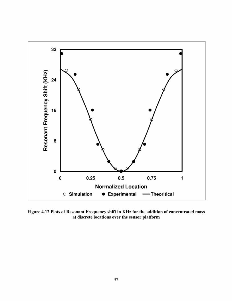
57
Figure 4.12 Plots of Resonant Frequency shift in KHz for the addition of concentrated mass
at discrete locations over the sensor platform
0
8
16
24
32
0 0.25 0.5 0.75 1
Reso
nan
t F
req
uen
cy S
hif
t (K
Hz)
Normalized Location
Simulation Experimental Theoritical
58
4.3 Influence of Physical Dimension
The previous sections involved the mass distribution and discrete location of concentrated mass
as factors affecting the resonance behavior of the sensor platform. Another important factor that
affects the resonance behavior of the system is the physical dimension of the sensor. This section
describes the influence of length and width of the sensor platform in resonance behavior. The
thickness is not separately explained since it would have the same effect as width over the
sensor’s behavior for the longitudinal vibration mode which would be explained in detail in the
width dependence section. Both the cases the mass attachment was very similar to the one we
discussed in the previous sections except for the increase in length or width of the sensor.
4.3.1 Length Dependence
Simulations were carried out to study the effect of variation in resonance behavior due to change
in dimensions of the sensor. Figure 4.12 show that variation in length of the sensor has a
dramatic effect on the frequency shift. When the sensor is subjected to Longitudinal vibration,
due to the sensor materials magnetic property the deformation occurs in the longitudinal
direction along the direction of the applied field. The larger the length of the sensor greater is the
sensitivity and hence greater resonant frequency shift for the same amount of mass.
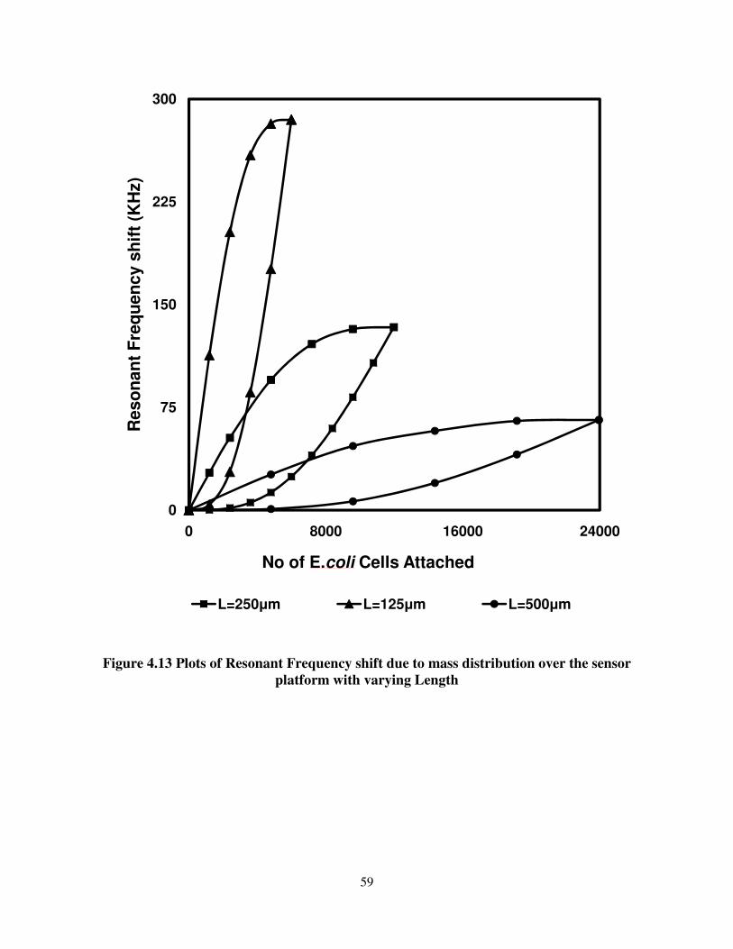
59
Figure 4.13 Plots of Resonant Frequency shift due to mass distribution over the sensor
platform with varying Length
0
75
150
225
300
0 8000 16000 24000
Reso
nan
t F
req
uen
cy s
hif
t (K
Hz)
No of E.coli Cells Attached
L=250µm L=125µm L=500µm
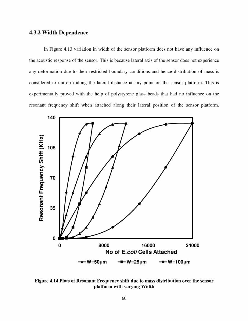
60
4.3.2 Width Dependence
In Figure 4.13 variation in width of the sensor platform does not have any influence on
the acoustic response of the sensor. This is because lateral axis of the sensor does not experience
any deformation due to their restricted boundary conditions and hence distribution of mass is
considered to uniform along the lateral distance at any point on the sensor platform. This is
experimentally proved with the help of polystyrene glass beads that had no influence on the
resonant frequency shift when attached along their lateral position of the sensor platform.
Figure 4.14 Plots of Resonant Frequency shift due to mass distribution over the sensor
platform with varying Width
0
35
70
105
140
0 8000 16000 24000
Reso
nan
t F
req
uen
cy S
hif
t (K
Hz)
No of E.coli Cells Attached
W=50µm W=25µm W=100µm
61
CHAPTER 5
CONCLUSION
A Model developed based on the acoustic response of Magentostrictive Sensor actuated
longitudinally with the modulated magnetic field. Numerical simulations and experimental
verifications were carried out with the predicted model considering the factors influencing the
resonance behavior of the sensor. The tolerance limit of frequency shift corresponding to the
distribution of mass, discrete position of the mass attached and the physical dimensions of the
sensor platform were determined in several ways. A Good agreement was found between these
results offering a good paradigm for detecting biological agents.
62
REFERENCES
1. Velusamy, V., et al., An overview of foodborne pathogen detection: In the perspective of
biosensors. Biotechnology Advances. 28(2): p. 232-254.
2. Mello, L.D. and L.T. Kubota, Review of the use of biosensors as analytical tools in the
food and drink industries. Food Chemistry, 2002. 77(2): p. 237-256.
3. Lazcka, O., F.J.D. Campo, and F.X. Muñoz, Pathogen detection: A perspective of
traditional methods and biosensors. Biosensors and Bioelectronics, 2007. 22(7): p. 1205-
1217.
4. Griffin, G.D., D.N. Stratis-Cullum, and S. Moselio, Biosensors, in Encyclopedia of
Microbiology. 2009, Academic Press: Oxford. p. 88-103.
5. Huang, S., et al., Sequential detection of Salmonella typhimurium and Bacillus anthracis
spores using magnetoelastic biosensors. Biosensors & Bioelectronics, 2009. 24(6): p.
1730-1736.
6. Ivnitski, D., et al., Biosensors for detection of pathogenic bacteria. Biosensors and
Bioelectronics, 1999. 14(7): p. 599-624.
7. Bhunia, A.K. and L.T. Steve, Biosensors and Bio[hyphen (true graphic)]Based Methods
for the Separation and Detection of Foodborne Pathogens, in Advances in Food and
Nutrition Research. 2008, Academic Press. p. 1-44.
8. Nayak, M., et al., Detection of microorganisms using biosensors--A smarter way towards
detection techniques. Biosensors and Bioelectronics, 2009. 25(4): p. 661-667.
9. Grate, J.W., S.J. Martin, and R.M. White, Acoustic-Wave Microsensors .1. Anal. Chem.,
1993. 65(21): p. A940.
63
10. Ballantine, D.S., et al., Acoustic Wave Sensors: Theory, Design, and Physical-chemical
applications. 1997, New York: Academic Press.
11. Thundat, T., P.I. Oden, and R.J. Warmack, Microcantilever sensors. Microscale
Thermophys. Engr., 1997. 1(3): p. 185.
12. Ilic, B., et al., Single cell detection with micromechanical oscillators. J. Vac. Sci. Tech.
B, 2001. 19(6): p. 2825.
13. S.Q., L., et al., Biosensor Based on Magnetostrictive Microcantilevers as a Sensor
Platform. Appl. Phys. Lett., 2006. 88: p. 073507.
14. Li, P., et al., A magnetoelectric energy harvester and management circuit for wireless
sensor network. Sensors and Actuators a-Physical. 157(1): p. 100-106.
15. http://www.metglas.com/.
16. Schmidt, S. and C.A. Grimes, Characterization of nano-dimensional thin-film elastic
moduli using magnetoelastic sensors. Sens. Act. A, 2001. 94(3): p. 189.
17. Wan, J., et al., Phage-Based Magnetoelastic Wireless Biosensors for Detecting Bacillus
Anthracis Spores. IEEE Sens. J., 2007. 7(3): p. 470-477.
18. Dover, J.E., et al., Recent advances in peptide probe-based biosensors for detection of
infectious agents. Journal of Microbiological Methods, 2009. 78(1): p. 10-19.
19. Ward, M.D. and D.A. Buttry, Insitu Interfacial Mass Detection with Piezoelectric
Transducers. Science, 1990. 249(4972): p. 1000.
20. Suwa, Y., et al., Study of Strain Sensor Using FeSiB Magnetostrictive Thin Film. Ieee
Transactions on Magnetics. 46(2): p. 666-669.
21. Raiteri, R., et al., Micromechanical cantilever-based biosensors. Sens. Act. B, 2001.
79(2-3): p. 115.
64
22. Bian, L.X., Y.M. Wen, and P. Li, The field dependence of magnetoelastic damping in
magnetostrictive material and its application in the magnetic field sensing. Acta Physica
Sinica. 59(2): p. 883-892.
23. Morshed, S., et al., Modifying Geometry to Enhance the Performance of Microcantilever-
Based Acoustic Sensors. Sensor Letters, 2009. 7(1): p. 38-41.
24. Morshed, S. and B.C. Prorok, Tailoring beam mechanics towards enhancing detection of
hazardous biological species. Experimental Mechanics, 2007. 47(3): p. 405-415.
25. Liang, C., S. Morshed, and B.C. Prorok, Correction for longitudinal mode vibration in
thin slender beams. Applied Physics Letters, 2007. 90(22).
26. Liang, C. and B.C. Prorok, Measuring the thin film elastic modulus with a
magnetostrictive sensor. Journal of Micromechanics and Microengineering, 2007. 17(4):
p. 709-716.
27. Park, C.S., et al., Dimensionally gradient magnetoelectric bimorph structure exhibiting
wide frequency and magnetic dc bias operating range. Journal of Applied Physics, 2009.
106(11).
28. Ong, K.G., et al., A rapid highly-sensitive endotoxin detection system. Biosens. Bioelec.,
2006. 21(12): p. 2270.
29. Cai, L., "Development of Bulk-scale and Thin film Magnetostrictive Sensor", in Materials
Engineering. 2007, Auburn University
Auburn. p. 1-258.
30. Mungle, C., C.A. Grimes, and W.R. Dreschel, Magnetic field tuning of the frequency-
temperature response of a magnetoelastic sensor. Sens. Act. A, 2002. 101(1-2): p. 143.
65
31. Stoyanov, P.G., et al., A remotely interrogatable sensor for chemical monitoring. IEEE
Trans. Mag., 1998. 34(4): p. 1315.
32. Guntupalli, R., et al., A Magnetoelastic Resonance Biosensor Immobilized with
Polyclonal Antibody for the Detection of Salmonella Typhimurium. Biosens. Bioelec.,
2007. 22(7): p. 1474-1479.
33. Huang, S., et al., The effect of annealing and gold deposition on the performance of
magnetoelastic biosensors. Materials Science & Engineering C-Biomimetic and
Supramolecular Systems, 2008. 28(3): p. 380-386.
34. Johnson, M.L., et al., A wireless biosensor using microfabricated phage-interfaced
magnetoelastic particles. Sens. Act. A, 2008. 144: p. 38.
35. Blevins, R.D., Formulas for natural frequency and mode shape. 2001, Malabar, FL.
USA: Krieger Publishing Company. pp. 183-184.