Embed Size (px)
Citation preview
Resource discovery over Peer-to-Peer networks for the creation of
dynamic virtual clusters
Carlos Paulo Ferreira Santos
Dissertation submitted to obtain the Master Degree in
Information Systems and Computer Engineering
Jury
Chairman: Prof. João Emílio Segurado Pavão Martins
Supervisor: Prof. Luís Manuel Antunes Veiga
Co-supervisor: Prof. João Nuno de Oliveira e Silva
Members: Prof. David Martins de Matos
October 2012

2

Acknowledgements
I would like to thank my supervisor, Luis Veiga, for still believing in me
and helping me finish this work through all hardships.
I would also like to thank my mother and my close friends for being
there for me.
Last, but definitely not least, I would like to thank my friend Irja for
helping me get through all bad moments, as well as being around for
the good moments. I would not be here without you.
3

4
Resumo
A importância da computação paralela e distribuida tem crescido nos
ultimos anos e a quantidade de tráfego em redes peer-to-peer tem
aumentado continuamente. Os métodos que estas aplicações usam
para manter a escalabilidade e atingir os seus objectivos podem ser
usados para melhorar a performance dos actuais sistemas baseados
em grids de forma a facilitar a criação e manutenção de clusters
virtuais dinâmicos, permitindo que estes possam atingir tamanhos
superiores ou funcionar de forma mais eficiente. Pretendemos
basear-nos nos pontos fortes dos sistemas peer-to-peer de forma a
criar um sistema capaz de dinâmicamente criar ou ajustar clusters
virtuais para a execução de aplicações distribuidas, permitindo dessa
forma uma maior disponibilidade destes mesmos clusters e ao
mesmo tempo diminuir os recursos computacionais desperdiçados.
Palavras-chave: Peer-to-peer, Grid computing, Virtual clusters,
Cycle-sharing
5

6
Abstract
The importance of cycle-sharing and distributed computing has
grown in the past years and the amount of internet traffic over peer-
to-peer networks is increasing. The methods that peer-to-peer
applications use to maintain scalability and perform their goals can
be used to improve upon current grid systems to facilitate the
creation and maintenance of dynamic virtual clusters allowing them
to grow further or perform better. We intend to draw upon the
strengths of peer-to and grid systems to create a system capable of
dynamically creating or adjusting virtual clusters for the execution of
distributed applications, thus allowing for higher cluster availability as
well as lessen the wasted computational resources.
Keywords: Peer-to-peer, Grid computing, Virtual clusters,
Cycle-sharing
7

8
Index
Table of Contents 1 Introduction .......................................................................................................... 2
1.1 Current Shortcomings ...................................................................................... 3
1.2 Objectives .......................................................................................................... 4
1.3 Document Structure ......................................................................................... 7
2 Related Work ........................................................................................................ 8
2.1 Peer-to-Peer ....................................................................................................... 8
2.1.1 Unstructured P2P ........................................................................................... 9
Napster ................................................................................................................. 9
FastTrack ........................................................................................................... 10
2.1.2 Structured P2P .............................................................................................. 11
Chord ................................................................................................................. 12
CAN ................................................................................................................... 13
Pastry ................................................................................................................. 14
Kademlia ............................................................................................................ 15
2.2 Grid systems .................................................................................................... 18
MPI .................................................................................................................... 21
Globus ................................................................................................................ 22
Condor ............................................................................................................... 23
Folding@home .................................................................................................. 25
Seti@home ........................................................................................................ 25
LHC Computing Grid ........................................................................................ 25
2.3 Analysis of the field ........................................................................................ 26
2.3.1 The grid and p2p convergence ..................................................................... 26
2.3.2 Cloud Computing ......................................................................................... 27
2.3.3 Virtual Clusters ............................................................................................. 28
Summary ............................................................................................................ 30
3 Solution .............................................................................................................. 31
3.1 Network System .............................................................................................. 31
3.2 Resource Discovery Protocol .......................................................................... 33
3.3 Cluster setup .................................................................................................... 35
3.4 Further detail and Implementation Issues ....................................................... 37
Main steps in resource discovery ...................................................................... 38
Cluster Deployment ........................................................................................... 41
Simulation .......................................................................................................... 41
Messages used ................................................................................................... 43
Summary ............................................................................................................ 45
4 Evaluation .......................................................................................................... 46
4.1 Join and leave .................................................................................................. 46
4.2 Candidate gathering ........................................................................................ 50
4.3 Dynamic cluster forming ................................................................................. 52
9
4.4 Message size .................................................................................................... 54
4.5 Size of the local data ....................................................................................... 56
4.6 Comparison to other P2P-Based systems ........................................................ 57
Message routing ................................................................................................. 57
Size of Local State ............................................................................................. 59
Request satisfaction ........................................................................................... 59
Performance under load ..................................................................................... 64
5 Conclusion .......................................................................................................... 68
10
Illustration IndexFigure 1: System overview.....................................................................................31
Figure 2: The entering of a node into the network.................................................32
Figure 3: Virtual appliance deployment.................................................................36
Figure 4: Changes in the overlay and its clusters...................................................36
Figure 5: Node representation in variant B............................................................39
Figure 6: Possible node representation of clock speed in variant C.......................40
Figure 7: Our class model......................................................................................42
Figure 8: Join message...........................................................................................43
Figure 9: Candidate collection message.................................................................43
Figure 10: Candidate list message..........................................................................44
Figure 11: Cluster formation message....................................................................44
Figure 12: Successful join message ......................................................................45
Figure 13: Number of messages taken for a Join message....................................47
Figure 14: Average number of messages taken for join message..........................48
Figure 15: Number of messages taken for a Join message with churn..................49
Figure 16: Number of messages taken for a candidate gathering message............51
Figure 17: Number of messages taken for a cluster forming message...................52
Figure 18: Comparison of messages required for growing candidate numbers.....53
Figure 19: Comparison of message routing in different systems...........................58
Figure 20: Average request satisfaction per overlay occupation, 100 000 nodes. .61
Figure 21: Average request satisfaction per overlay occupation, 10 000 nodes... .62
Figure 22: Average request satisfaction per overlay occupation, 1000 nodes.......62
Figure 23: Average request satisfaction per overlay occupation, 100 nodes.........63
Figure 24a: Join message comparison....................................................................65
Figure 24b: Join message comparison...................................................................65
Figure 25a: Candidate gathering message comparison..........................................66
Figure 25b: Candidate gathering message comparison..........................................67
1

1 Introduction
In the ever-evolving modern world, one of the few constant facts of the
computer industry has been growth. This growth manifests itself both in terms of
computationally more demanding applications as well as a higher availability of
computational resources.
One would think these patterns of growth would neatly overlap, yet that is not
so. A high amount of computer cycles are being wasted at all times all over the
world, and yet, at the same time there are applications that have a strict demand
for computational power that requires more than a simple computer's effort to
satisfy.
Over the past 20 or so years, several approaches to this problem have been
created. Initially most heavy computational processes were handled by
supercomputers and mainframes, but this solution was both expensive and
inherently generated inefficiency.
With the passing of time the concept of a computational cluster became the
norm. A group of machines, similar both in hardware and software specifications,
but also connected by high-throughput and high-availability networks, solely
dedicated to the solving of a common problem through the usage of distributed
and shared computing mechanisms.
2
1.1 Current Shortcomings
However, while locally capable of providing for the needs of any entity requiring
such form of computational power, the several existing approaches still failed to
provide a solution except for the most wealthy and stable of companies[9]. The
common user was still without a solution, the vast resources of the internet were
still not being used, and above all, there was still a high amount of computational
power that was wasted, not only during idle times in computer clusters, but also
in the raw untapped power of millions of personal computers and other
computational devices (such as the ever popular portable cellphones, hand-held
devices, etc.) all over the world connected to the internet[26].
Several partial solutions appeared with the passing of time, each focusing on a
certain approach and method to solve the challenges required to implement a
platform that would both maximize computational power available as well as
minimize resource waste.
The concept of distributed and parallel computing itself is one of the interesting
points that evolved alongside the clustering paradigm. Cycle-sharing and Grid
computing are different approaches to this concept, each with their own goals
and constraints. These constraints that still prevent the public from having access
to proper clustering tools. In a way, public computing and computer clusters are
still like two islands in a sea, totally separate, due to the lack of tools to overcome
such constraints. Should a tool arise that could allow for the dynamic creation
and alteration of clusters based on a peer-to-peer network, we could finally reach
the goal of allowing the computational power of clusters to the general public.
3
1.2 Objectives
Our goal is to design a system based on a public, peer-to-peer overlay network of
nodes representing computers offering or needing resources that can on a per-
request basis locate a list of the best candidates for the creation of a virtual
cluster from the nodes present in the network. With this list we will make a
choice of the exact machines that will be part of the cluster and finally create the
cluster itself, always maintaining the capability of adjusting its size or members.
This system must be able to:
• Allow the soft and controlled entrance and exit of nodes from the
network.
• Locate resources in useful time, ensuring that if a resource exists, it can
be found
• Take into consideration each machine's specifications including CPU type,
clock speed, core availability as well as available bandwidth
• Allow each request to specify QoS1-level metrics to refine the search and
provide the best candidates for a cluster.
• Be capable of finding a cluster of the appropriate size and specifications
to meet the needs of the request
• Maintain a high level of scalability and reduced bottlenecks/points of
failure.
• Create and maintain a cluster from heterogeneous machines if necessary
• Initiate a cluster dynamically, at request execution time
1 Quality-of-service
4
In order to do this, we will create an approach that involves both a P2P2-based
protocol for resource discovery, a P2P-based node handling system and an
application for the deployment of the code to be executed on the recently
created virtual cluster.
This will solve the major issues highlighted in the previous section, our approach
will perform such tasks in an efficient way, making use of resources located not
only in fixed, easy to access networks but mainly via perishable networks like the
internet. We will present a system that allows a user to share local resources, set
up QOS levels in several aspects in order to locate a machine or group of
machines currently available that best fits the execution of an application as well
as actually relaying the execution of the application in that machine or virtual
cluster.
To achieve this, there are three main problems to solve. The first of those lies
with the nature of the network wherein we will locate our resources. The
internet is not without fails and faults, and even though its reliability (and
availability) has greatly increased in the past years, we cannot assume a node
present at a time to be available at another time.
Our system must be able to allow a node to make itself known and announce its
available resources without generating an exponential amount of control
messages in order to ensure a capacity for scaling.
The second issue is directly linked with the first one. Our protocol must be able to
locate resources that have been announced that fit the criteria defined in the
QoS specifications. The same care must be shown in order to avoid flooding the
network, but also we have to pay attention to the amount of time spent locating
the “perfect” resources (that match the request's specifications exactly), and
whether locating them is feasible.
2 Peer-to-peer
5

The third and final issue appears once we have obtained a list of candidates for
execution of the required application. From that list, we will have to choose a
machine or group of machines that can better satisfy the QoS requirements and
start a virtual cluster for the execution of the code. Those resources will have to
be reserved, execute the code, the results of the execution must be gathered and
assembled and then the resources should be freed, to be reused. This can be
achieved by using an appropriate tool (like a small applet or virtual appliance)
that is dynamically deployed onto the machines of the selected nodes.
In further detail, our resource-discovery protocol will be based on a structured
peer-to-peer approach and will be oriented towards locating machines that can,
either partially or fully, satisfy the QoS-level metrics presented by the request.
These metrics can include characteristics such as the machines' number of CPUs,
their CPU availability, available RAM, storage space, network latency and/or
bandwidth available, among others.
The system we will design for handling the entrance, exit and maintenance of
nodes in the network will be based in a peer-to-peer approach to ensure a low
amount of overhead generated by control messages. It will have to maintain the
data on resources, node availability and characteristics in order to sustain the
node network's health as well as feed the resource discovery protocol.
Finally, the prototype application will both serve to deploy the code to be
executed onto the target dynamically created cluster and provide an interface for
the use of our proposed system.
This work was carried out within the scope and partially supported by national
funds through FCT – Fundação para a Ciência e a Tecnologia, under projects
PTDC/EIA-EIA/102250/2008 and PEst-OE/EEI/LA0021/2011.
6

1.3 Document Structure
We have discussed the objectives of our own approach in Section 1.1 A global
analysis of previous approaches will be presented in Chapter 2. Such analysis will
be accompanied by a brief evaluation and analysis of a few strengths and
weaknesses of such approaches, what they are lacking and where they succeed.
Chapter 3 contains the description of our implementation and how we overcome
the difficulties of our approach while capitalizing on the strengths of our program
to solve the two major issues ahead of us. We evaluate the system implemented
in Chapter 4 through several methods, analyzing its practical results and both
comparing it against our own expectations as well as some other already existing
systems. This document wraps up with Chapter 5 where we present a short
reflection of the results of our labor and the impact the solution could have in the
current computing environments.
7

2 Related Work
Isaac Newton once said “If I have seen further it is only by standing on the
shoulders of giants.“ and we are in the same position. Our work is based on
gradual evolution in the field, both in the academic world and in the computer
industry. In this chapter we will describe the evolution in two main fields within
which our work is based. The first one is regarding resource discovery in peer-to-
peer/grid networks while the second one relates to the creation of dynamic
clusters itself.
The following subsections contain an analysis of the origin and evolution of those
technologies, as well a analyze why they succeeded and failed.
2.1 Peer-to-Peer
Peer to peer (or more commonly P2P) is a concept where resources are shared
among several nodes in a network, be those resources tasks, information or
storage. The networks based on this concept can be both structured and
unstructured. We will first give an example of unstructured ones.
These systems share responsibilities amongst the nodes and allow for far greater
resource availability than existed in previous single-point or centralized
approaches.
A peer to peer system is characterized by its level of decentralization, which is
how distant from the ideal that all nodes in the network are equal. This affects
not only the homogeneity of the nodes in the network but also the degree of
scalability and performance issues that might arise.
8
Another important point in these systems is resource discovery, or the method
for which a node discovers other nodes/resources in nodes. This can greatly
affect the performance of a system, to the point of actually making it unusable in
practice.
One issue concerning these systems is the joining and leaving of nodes from the
network. This is directly tied to its level of decentralization, but is independent
enough that merits mentioning. Although it has only a partial impact on
scalability, it can greatly hinder the performance of a system if not handled
correctly.
2.1.1 Unstructured P2P
This concept was first made famous by the application Napster that quickly
accrued upwards of 80 million files shared between 1999 and 2001[27]. Napster,
however, is unlike more modern P2P implementations in the fact that it was a not
a fully decentralized technology, using superservers to direct and control
entrance into the network, resource discovery and node publication, among
other tasks.
Napster
Napster uses in fact a Hybrid Decentralized Architecture[5] which uses the
aforementioned superserver in addition to normal peer nodes in a network. This
particular feature is one of the weaknesses of this type of approach offering an
individual point where failure or fault greatly compromises the P2P network, as
well as offering a bottleneck that can greatly affect scalability of the system.
9

This approach in fact limits one of the strong points of P2P systems: scalability.
More modern approaches use one of two different P2P types, which vary exactly
in the equality of peers within the network. A Partially Centralized Architecture[5]
[12], such as the one used by the FastTrack protocol (as used in KaZaa or ED2K
based systems[15]) is based on the existence of some peers that accumulate
more responsibility than that of the usual client, and thus also have tasks of
control and organization of the network.
FastTrack
Unlike Napster's approach, the lack of a central server means there is no
bottleneck, and the tolerance for fails and faults is much higher. The sudden
absence of one of these superpeers does not compromise the network. If it is
necessary, a new superpeer can be elected to take the place of the previous one,
or in some cases another already existing superpeer can take over for the absent
one. In any case, these peers are required to present certain characteristics in
order to be promoted to a superpeer, both in terms of computational power as
well as bandwidth available to them.
The final type of P2P system is the Purely Decentralized Architecture[12][1]. This
system presents true equality among peers, not using superpeers or centralized
servers. For a new node to join a network of this type, he simply needs to know
the address of a node already in the network, and the system itself
accommodates for the new node and spreads the information of its existence.
While this may seem to offer less bottlenecks than the previous two types, there
is an issue with resource discovery.
10
Due to the lack of nodes with the responsibility of containing information on the
resources present in the network, a much higher amount of control messages
might be required in the system.
Traditionally the spreading and discovery of resources was handled by flooding
the network. The evolution of these systems started using other methods such as
random walks [20] and Distributed Hash Tables[17][11] (as seen in the
Bittorrent[23] protocol and several of the structured networks present in the
following subsection 2.3. )
2.1.2 Structured P2P
Unlike the peer to peer based systems described in the previous subsection,
structured peer to peer architectures use a rigid organization to govern the nodes
within the network. This well-defined structure allows some knowledge over the
nodes to be passed onto their itself as well as both ensure that resource locating
algorithms do not flood the network and that if a resource exists, it is found in a
well-known and predictable number of steps[14].
Examples of systems that use a structured peer to peer approach are for
example, Chord [8] and CAN [4]. There are some systems such as Pastry [19] and
Kademlia [16] that use portions of both unstructured and structured systems, but
in their essence function as structured approaches. The great advantage these
approaches have over an unstructured approach is the control over node joining
and content that lies within the node structure, ensuring both a lower amount of
control messages as well as faster (or at least more certain) searches.
11
Chord
Chord was one of the first structured peer to peer systems, developed at MIT,
and uses a Distributed Hash Table to store pairs of keys and values. Each node
stores all values for any keys he is responsible for, and the system enforces how
each key is given to each node.
Resource discovery in Chord takes two steps: first you locate the node that is
responsible for the key, then you locate the key (and appropriate value) in such a
node. Like many structured approaches of this type, the nodes in Chord are
structured in a figurative directed circle. Each node has another node as a
successor and one as a predecessor in the circle.
In order for chord to function, the system uses a consistent-hashing system to
generate a unique identifier with a length of N bits. The maximum number of
nodes in a Chord circle is 2n nodes, and each of these is responsible for a number
of keys equal to the total number of keys divided by the number of nodes.
To ensure safe departure from the network, each node has not only information
of its successor, but also information on a few of the following nodes, ensuring
that the circle is not broken upon network or node failure. Whenever a new node
joins the network, the responsibility of each node is recalculated to ensure an
even distribution of keys.
12
CAN
CAN (short for Content Addressable Network) is another DHT-based structured
P2P system. Unlike chord, the nodes are not sorted in a circular fashion. CAN
interprets the node space as a N-Dimensional axial system.
Nodes are assigned coordinates as if they were a point in the axial system and
each node is assigned a partition of the total dimension that the node becomes
responsible for.
Each node contains a list of its neighbor nodes as well as their IP addresses and
maintains this information in a routing table of sorts. Also unlike Chord, a node's
entrance into the network causes not a calibration of the whole weight, but only
a split in one of the spaces assigned to a node. The new node contacts a node
already present in the network and discovers a node (either by picking random
coordinates in the system) that is responsible for a certain amount of space. That
node splits his space into two between itself and the new node, and informs the
neighboring nodes of the new responsibilities. The information is then
propagated across the network.
This small change causes a much smaller amount of overhead (when compared
to Chord) in networks with high amounts of nodes and keys, but conversely does
not guarantee that the keys are evenly distributed as Chord does.
The process for a node's departure from the network is more complex. There has
to be a control mechanism that periodically probes the nodes for livelihood.
Once a node leaves the network, its space is merged with one of its neighbor
nodes and that information is once again propagated to the merged node's
neighbors and the network.
13
To ensure that the routing protocol in CAN is obeyed, the choice of which
neighbor gets the responsibility over the space previously assigned to the node
that left follows strict rules regarding the shape of the final space. If no merge is
possible, then the neighbor node with the smallest space is assigned
responsibility over the departed node's space as well.
The actual of a resource is handled based on the resource's coordinates in the
axial system. From any node, you simply move the request onto the neighboring
node that is in the direction of the resource's , and the request moves forward in
this fashion until the is finally reached.
Pastry
Pastry is in many ways similar to Chord. Nodes are also arranged in a circle, and
the system also uses a Dynamic Hash Table to store key-value pairs. The main
difference between the two are the Ids that each system handles.
Pastry uses a 128-bit ID setup that represents a position in the circle. Node IDs
are assigned at random and on top of the circular node setting pastry uses an
external routing overlay network. This overlay maintains information on node
“proximity” (be it through the existence of a low amount of hops between them,
low latency, etc) in a list of neighbor nodes.
14
Each node also maintains a list of leaf nodes which are the closest nodes to itself
in terms of node ID, totally disregarding the metric. The routing list basically looks
at each 128 bit key as a length of digits or characters as if it were a string, and
sets farther nodes (in terms of the metric) to strings that have only 1 of the digits
or characters in common to it, while nodes “closer” might share more characters
in common. For example, given a node with key ABCD, the node FGHD is farther
away than the node CBCD.
The actual routing of a message takes multiple steps. If a node wants to send a
message to a certain key, that node sends it directly to that space. The node with
the ID closest to it on the circle then scans its leaf nodes to check for the key
being present there. Should it be there, the message is delivered. Should the key
be absent, the node's routing table is consulted to attempt to find a node with
the a longer string in common with the target key.
This structure allows real life constraints such as bandwidth and round trip times
to determine proximity in nodes, which can greatly increase the performance of
such a system.
Kademlia
Kademlia[16], like Chord and Pastry before it, also uses a Dynamic Hash Table,
but in this case the hashing is directly tied to the IDs of the nodes. In a Kademlia
network, resource location is an iterative, gradual approach. Every step of this
process attempts to find “closer” nodes to the target key, and proximity is
determined by a simple hashing of node IDs.
15
Each of these steps ensures that either a better match is found, or that either the
node is absent or that we've found the key being procured. Another large
differentiating feature in Kademlia is that the distance of nodes is kept in lists by
each node. There is one list for each bit in the node ID, so if there were 32 bits in
such an id, there would be 32 lists kept in each node. The first one contains the
nodes farthest away from this one, and each subsequent list contains nodes
closer. These lists are updated as nodes are encountered, which generates a very
low overhead and keeps the routing list fresh.
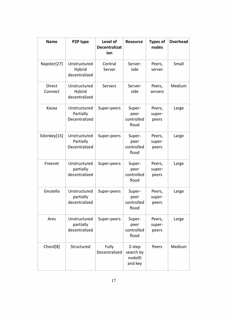
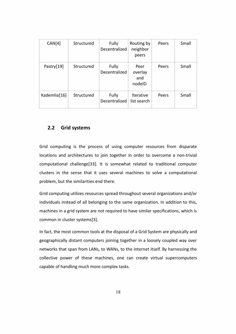
For ease of reference, we will provide a comparison table between the systems
described above, containing a few of the main characteristics of each.
We define overhead in this table as the amount of control and system messages
necessary to maintain the correct state of the system, its nodes and the
resources available. Ideally in a single-machine system, these are nearly
nonexistent. The lower the overhead resulting from these messages, the
smoother the system scales with a growing number of nodes.
This is a defining point of any system, as it can determine the capability of our
system to accompany a large growth in the number of nodes. The control
messages usually stem from resource requests and finds, file transfers, among
others.
Also, when referring to “servers”, these are specialized machines, not selected
from normal nodes, and multiple in number, as opposite to super-peers which
can sometimes be drawn from the normal node pool. These specialized machines
are centralized in fashion and predetermined by the system itself before the
network overlay is established.
16
Name P2P type Level of
Decentralizat
ion
Resource Types of
nodes
Overhead
Napster[27] Unstructured
Hybrid
decentralized
Central
Server
Server-
side
Peers,
server
Small
Direct
Connect
Unstructured
Hybrid
decentralized
Servers Server-
side
Peers,
servers
Medium
Kazaa Unstructured
Partially
Decentralized
Super-peers Super-
peer
controlled
flood
Peers,
super-
peers
Large
Edonkey[15] Unstructured
Partially
Decentralized
Super-peers Super-
peer
controlled
flood
Peers,
super-
peers
Large
Freenet Unstructured
partially
decentralized
Super-peers Super-
peer
controlled
flood
Peers,
super-
peers
Large
Gnutella Unstructured
partially
decentralized
Super-peers Super-
peer
controlled
flood
Peers,
super-
peers
Large
Ares Unstructured
partially
decentralized
Super-peers Super-
peer
controlled
flood
Peers,
super-
peers
Large
Chord[8] Structured Fully
Decentralized
2-step
search by
nodeID
and key
Peers Medium
17
CAN[4] Structured Fully
Decentralized
Routing by
neighbor
peers
Peers Small
Pastry[19] Structured Fully
Decentralized
Peer
overlay
and
nodeID
Peers Small
Kademlia[16] Structured Fully
Decentralized
Iterative
list search
Peers Small
2.2 Grid systems
Grid computing is the process of using computer resources from disparate
locations and architectures to join together in order to overcome a non-trivial
computational challenge[33]. It is somewhat related to traditional computer
clusters in the sense that it uses several machines to solve a computational
problem, but the similarities end there.
Grid computing utilizes resources spread throughout several organizations and/or
individuals instead of all belonging to the same organization. In addition to this,
machines in a grid system are not required to have similar specifications, which is
common in cluster systems[3].
In fact, the most common tools at the disposal of a Grid System are physically and
geographically distant computers joining together in a loosely coupled way over
networks that span from LANs, to WANs, to the internet itself. By harnessing the
collective power of these machines, one can create virtual supercomputers
capable of handling much more complex tasks.
18
The immediate comparison to traditional cluster systems shows pros and cons on
both sides. The typical cluster system can take a greater advantage of the
machines at its disposal, but requires a large investment in planning and
hardware. Cluster systems by definition may are only limited the machines
available and the network connecting them, but can join together a much larger
amount of machines and thus derive more computational power from them.
One of the more modern details regarding Grid systems is the usage of
established middleware to deploy (and possibly partition) or integrate with the
code to be executed among the machines that will perform that task, thus
reducing the system's need to focus on that point.
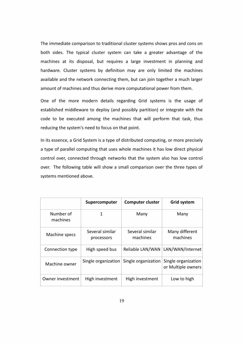
In its essence, a Grid System is a type of distributed computing, or more precisely
a type of parallel computing that uses whole machines it has low direct physical
control over, connected through networks that the system also has low control
over. The following table will show a small comparison over the three types of
systems mentioned above.
Supercomputer Computer cluster Grid system
Number of
machines
1 Many Many
Machine specsSeveral similar
processors
Several similar
machines
Many different
machines
Connection type High speed bus Reliable LAN/WAN LAN/WAN/Internet
Machine ownerSingle organization Single organization Single organization
or Multiple owners
Owner investment High investment High investment Low to high
19

investment
Performance
potential
High High Average to very
high
Duration of service Long term Long term Task oriented
Overhead Nearly nonexistent Small Medium
Resource wasting Idle periods Idle periods Very small
Grid systems as a whole have been used in the solving of several computationally
intensive problems in several ares of science and academics, from the discovery
of new medicine and drugs to the execution of complex mathematical
calculations.
One of the advantages of this approach is that the individual machines that form
the grid can be purchased independently of each other, on a per-need basis, and
later be used in the virtual supercomputer created by the grid. The obvious
advantage here lies with the low initial cost and investment if the requirements
are not too extreme. [25]
Many small companies requiring higher computational power were for several
years barred from attaining it due to the steep initial investment costs inherent to
the acquisition of a supercomputer or the creation of a cluster. Grid systems
present themselves as the cost-effective solution as well as having the potential
for very high computational performance.
However, not all is advantageous when it comes to Grids. Due to the very nature
of the machines involved, individual nodes cannot be relied upon as machines in
a cluster can. Not only can the nodes themselves be unreliable, the network
connecting them may present failures as well. To prevent compromising the job
being done, the system must apply strict measures to prevent a single machine's
20
failure or absence from critically affecting a job that is underway.
A certain type of distributed computing that is a particular form of grid systems is
what is called Cycle-scavenging[7] (sometimes called cycle-stealing or public
computing). This is what is behind the many well-known volunteer computing
programs like Folding@home and Seti@home. The latter one has in the past
years changed its system to use BOINC, one of the several grid-oriented
middleware applications available.
The applications using cycle-scavenging are typically installed in a voluntary
fashion by the machine's owner and run when the computer itself is idle. There is
little cost to the machine's owner, and these applications serve purposes of
general interest. The main goal of reducing idle times in computers is achieved by
these applications, but still the goal of allowing supercomputing to be accessible
to the general public is still unsatisfied.
However, grid computing is becoming more mainstream than simple cycle-
scavenging programs. CERN has become a great proponent of Grid systems and
there are several initiatives throughout Europe that aim to further the Grid
system's evolution.
We will now present a more closer look at some examples of systems using grid
technologies as well as cycle-scavenging/public computing.
MPI
Message Parsing Interface is a protocol specification designed to allow computer
processes to communicate with each other. It was first announced in draft form
in 1994 and aimed at being used in distributed and parallel computing in systems
where the costs for accessing remote memory are too high[29] due to the way
they are connected.
21
It is easy to see the importance such a protocol can have in distributed
computing systems like clusters and grids, and the impact MPI had can quickly be
seen in the fact that even though it is not considered a standard, it has all but
become a de facto one in today's parallel and distributed computing world, being
used in large amount of the appropriate systems.
Being only a specification, MPI allows several implementations to exist, in several
programming languages as well as having two different versions, with different
scopes. MPI-1.2 (commonly shortened to MPI-1) is more focused on the actual
message passing while MPI-2 also includes parallel I/O, dynamic process
management and remote memory operations[28].
MPI-1 focuses mostly on topology, communication and synchronization between
processes. It achieves this by using unique objects and concepts (e.g. process
barriers) for each specialized situation, from using “communicator” objects to
handle multiple processes to mechanisms aimed at passing a message from a
particular process to another (or broadcasting it to all other). It also defines
specific data types for usage with the specification.
Globus
The Globus toolkit[13] is a set of open source tools for the creation of computing
grids. It was developed from 1995 onwards by an international association that
eventually came to form the Globus Alliance in 2003.
22

It has a specialized tool for resource management called GRAM[2] (Globus
Resource Al and Management protocol). GRAM can handle most basic job-
related functions as well as more advanced functions such as managing
credentials and monitoring the status of resources. GRAM receives a job as a
single submission directed at a single computational resource and can provide
not only input files but also output files for the result.
For the management of credentials and security, Globus uses a tool called GSI
(Grid Security Interface). GSI ensures that data is not tampered with, can be
authenticated and is read only by those that have a responsibility with it. Within
the Globus toolkit a legacy tool called MDS-2 (Monitoring and Discovery Services)
for the monitoring of computer resources in the grid, but support for this tool is
scheduled to be stopped and the tool removed from the kit.
Condor
Condor[10] is a software framework for distributed computing aimed at
distributing the workload over a dedicated cluster of computers, but may also be
used to draw unused computer cycles from idle machines. It was developed in
the University of Wisconsin in Madison as a means to tackle the problems
inherent to distributed computing.
One of Condor's advantages is the seamless integration of heterogeneous and
disparate resources, from clusters to regular desktop computers. This in part
derives from the developer's strong focus in the philosophy of flexibility as a
requirement for a system of this type.
The Condor system uses a component called Condor-G as an interface to
communicate with Grid resources (and also Cloud resources). Its name derives
from that of Globus (mentioned further in this document) which was the Grid
creation method Condor used at first.
23
Condor supports the MPI specification but also has a proprietary library called
Master Worker. MW is aimed at tasks that require a substantially higher degree
of parallelism.
Boinc
Boinc is a Grid middleware application developed in the Berkeley University of
California in 20022. its original goal was as a platform to support Seti@home but
it quickly outgrew that goal and started being used in a more widespread fashion
around the world. According to statistics publicized monthly, the Boinc-powered
virtual supercomputer has risen above 4 000 Tera flops (average) of
computational power3, spread out over more than 20 different projects.
This is more than twice the fastest supercomputer available at the time of writing
this document (the Jaguar-Cray XT5 HE, at approximately 1750 Tera flops4), which
is a number that not only proves the efficiency and potential of Grids, it also
shows their rapid exponential growth, reaching this peak in only 6 years.
If we consider peaks of performance instead of averages, the Boinc virtual
supercomputer has achieved over 5 400 Tera flops.
Boinc itself is a free mechanism for anyone that wishes to start a volunteer
computing system, and is mostly used for scientific purposes and is currently the
largest open Grid system in existence.
2:BOINC website, http://boinc.berkeley.edu/
3: BOINC statistics http://boincstats.com/stats/project_graph.php?pr=bo
4: Top 500 Supercomputer List http://www.top500.org/lists/2010/06
24
Folding@home
Folding@home is a cycle-scavenging system designed in the Stanford University
in California in 2000 to model protein folding in order to gain insight over several
diseases and medicine5.
Much like any cycle-scavenging system, it relies on a user installing its client in a
machine so that it can access the machine. It has achieved a peak of 5 600 Tera
flops but averages out at approximately 5 000 Tera flops divided over seven
different “cores” of research, each with their own peculiarities.
Seti@home
Seti@home is a cycle-scavenging system released in 1999 destined to scan data
obtained in the Arecibo astronomical observatory in order to attempt to find
hints at the existence of extra-terrestrial life6.
From 2005 onwards, Seti@home started using the Boinc platform instead of its
own proprietary system. It is currently averaging approximately 730 teraflops, or
approximately 17% of the Boinc virtual supercomputer.
LHC Computing Grid
As mentioned above, CERN has embraced Grid systems as an answer to the large
computational power required to interpret the immense amount of data being
gathered from the LHC experiments[6].
5: Folding@home http://folding.stanford.edu/English/License
6: Seti@home http://seticlassic.ssl.berkeley.edu/about_seti/about_seti_at_home_4.html
25
It was started at the end of 2008 and currently has participating nodes spread
over three continents and contains machines of over 140 different institutions.
2.3 Analysis of the field
Having looked at several examples of related work, we need to look into our
system's direct relationships to those examples, as well as their future heading
given the current technological conjecture.
2.3.1 The grid and p2p convergence
At the current point of time, peer to peer systems and grid systems are largely
independent. They were, after all, developed independently and aimed to solve
different goals. Yet, the evolution of both systems may show a confluence
between them in the near future[18].
As grid systems grow, scalability issues will require them to start using tools
commonly used in peer-to-peer systems to avoid bottlenecks and slowdowns as
well as possible points of failure. On the other hand, as peer to peer systems
become larger in size and attempt to claim more possible uses, they too start
using structured models commonly seen in Grid systems.
One could say that eventually there will cease to be any distinction between the
two types of systems, and that a single, common architecture will be present to
fulfill the goals of both systems: resource sharing (be it in terms of computational
power, data storage, or data itself) and the avoidance of resource wasting. How
soon it happens is still unknown, but it is a near certainty of modern advances.
26

2.3.2 Cloud Computing
One unavoidable concept in today's distributed computing world is that of cloud
computing. The company Amazon is one of the entities most responsible for the
appearance of the concept of cloud computing.
It came to be during the company's internal hardware system restructure, an
action whose goal was to minimize the wasted computational resources inherent
to the company's everyday work.
A company study showed that sometimes only 10% of the machine's total
capacity was being used. During attempts to solve that, the idea of a pool of
computational resources evolved into the modern notion of the cloud. Of course,
had it remained simply a tool for the internal use of the company, the cloud
would not be a topic as well known as it is today. In 2006, Amazon started to
provide cloud computing to the outside public8.
A more careful look at the cloud shows it using concepts already present both in
grid systems, cluster systems and public computing, but with a different
implementation and a more restricted set of premisses.
From the point of view of a regular user, cloud computing seems to solve all the
tasks we set forth to achieve with this work, but after careful analysis, it is not so.
Cloud computing as it is currently pictured ends the client user's control after the
request is made and any decision on the cluster is done without the client user's
interference. While it does add to general agility for typical use, it denies the user
the capacity of adjusting the clusters to his own needs.
8: The Amazon elastic cloud, http://aws.amazon.com/ec2/
27

Furthermore, the cloud is still closed in the sense that the machines providing the
computational capabilities will not request more capacity themselves, and that a
typical user cannot provide his own unused computer cycles to someone else.
These points are strong enough that a niche for our work exists, and this niche is
substantial enough that it warrants a solution, a proper answer to the issue at
hand.
2.3.3 Virtual Clusters
The concept of a virtual cluster[24] is tied directly to that of the traditional
computer cluster. Originally, clusters were groups of similar computers belonging
to a single organization in order to either improve performance by spreading
computational load, diminish network load impact by spreading traffic around or
ensuring a higher availability of data. These computers were traditionally
connected by high-bandwidth networks, had similar specifications and were
closely monitored and under strict organization.
Virtual clusters deviate from tradition by being more loosely coupled and not
necessarily physically close to each other. In addition, the biggest diverging point
is that while clusters are permanently assigned to their particular job, machines
participating in a virtual cluster might be performing that job only a shorter
period of time, being released afterward.
In addition to the constraints and concerns already present in the creation of a
normal cluster, some additional issues arise when we observe the creation of
dynamic virtual clusters. Some of those issues stem from the difference in
networks present between the nodes of the cluster while others arise from the
lack of homogeneity between nodes.
28
The network connecting the machines itself adds additional focus points. In
applications that require a hefty amount of data transfer between them, high
bandwidth may be required, and that can influence the performance of the
virtual cluster, while on the other hand if a small amount of data is passed
amongst nodes, but it is done fairly often, a globally low latency becomes the
priority.
Additionally, the necessity for the cluster to be dynamic or elastic, that is, being
able to alter its size or nodes at will, requires control mechanisms aimed at
allowing departure and entrance into the cluster as well as job management and
handling throughout the changing node network. This management must be able
to provide strict control of the resources within the cluster.
A bottom-up approach to virtual clusters would lead us first to the actual creation
of the cluster. Krsul [32] described a way to create virtual clusters by using virtual
machines. A single virtual machine image would be cloned throughout the
machines belonging to the cluster. This virtual machine would then receive a
directed acyclical graph containing configuration instructions and with them the
machine would be set up. Foster [31] provided a solution to the same problem by
introducing the concept of a virtual workspace. This virtual workspace is nothing
but another virtual machine which instead receives its configuration instructions
as an argument and then is deployed to the actual physical resources in the
cluster.
While both above solutions are fine for a low number of machines, they would
not scale well with a sufficiently high number of machines, and alternatives for
larger clusters were created [30]. Here, the deployment itself is accelerated by
means of virtual disk caches (and other techniques) which contain any and all
required software, thus greatly hastening the initial deployment.
29
Past the initial deployment step, the existence of a virtual cluster requires
managing of jobs and resources. To do so, a virtual cluster requires the existence
of a Resource Managing System (RMS) that can assign jobs, extract job results,
control node absence and presence, maintain the integrity of the computational
exercise being done and ensure the general stability of the virtual cluster[21].
To do so, the RMS must, upon reception of a request, estimate the impact the
request would have on each machine, and then generate a plan for job
distribution and handling amongst the machines in the cluster. In addition, the
RMS must also provide the security aspect of a request, by authenticating
credentials and ensuring data confidentiality within the cluster.
Summary
In this chapter we presented several existing systems and briefly explained the
essential points in how they function. For both grid and peer-to-peer systems, we
emphasized their strengths and weaknesses, drawing lessons from the way they
capitalize on the former and mitigate on the later, in order to inspire, properly
define and fine tune our system. We shall now proceed to describe our solution
and how it was influenced by preexisting work in the next chapter.
30

3 Solution
The design presented in this paper focuses on three individual parts as
mentioned in Chapter 2. In this chapter we will provide a more detailed look into
both our system and the inherent protocol it uses to achieve its goals. In general
our system will provide means for a new node to join a network in order to be
able to utilize resources on remote computers as well as allow his own resources
to be used by remote requests.
3.1 Network System
Figure 1: System overview
The figure above shows the overview of our system and a general outline of the
several actions in a typical request. To be able to perform these actions, the three
individual parts (the peer-to-peer network system, the resource protocol and the
clustering virtual application) of our work must interact and communicate
amongst themselves in well-defined ways.
A more detailed description of these parts and their interfaces will now be
depicted.
31

Our system is based on a structured peer-to-peer network of nodes. We choose
this type of network to allow quick and efficient of resources and swift routing to
specific nodes, thus promoting scalability and still maintaining the decentralized
architecture. We will model our system in PeerSim, providing the added
functionality for node joining and leaving as well as resource availability control
and job request specification.
The system will allow a machine to join a network by simply knowing the IP or
address of a node already in the network (as depicted in Figure 2), and will
accommodate the new node in its overlay. Both the departure of a node (loss of
available resources) and the joining of one (increase in available resources) will
be propagated throughout the network in a controlled way in order to not flood
the system.
Figure 2: The entering of a node into the network.
32

3.2 Resource Discovery Protocol
The actual submission of a job request can be accompanied by several quality of
service metrics. A request can be made for a cluster of a specific number of
computers and values to each of the QoS metrics can be provided with the
request to later allow our resource discovery protocol to refine the list of
candidates and correctly estimate the machines that best fit the requirements of
the request. For instance, we could request a cluster composed of 6 machines
where we would give a very high weight to a low latency in the network
connections between them as well as the individual machines' CPU type and
number of cores, in order to accommodate an application with low size messages
being swapped among the machines in the cluster.
After a request is submitted, our resource protocol sets in, working on the node
network maintained by our system and will attempt to locate resources that
either fit the request's QoS metrics completely, or at least locate machines that
partially fit the request, all the while maximizing their adaptation to the task.
Considering the heterogeneous nature of the nodes in the network, it is most
likely that only partial matches can be found[22], but the capacity for this
protocol to maximize the cluster's capacities to fit the request are a crucial point.
Thus, we allow each node to, upon request submission, specify minimum
thresholds for both partial and global resource satisfaction.
The protocol itself will be modeled in the form of Java classes tailored to fit our
system using PeerSim for simulation purposes. The protocol's work has two
steps. In the first step, the protocol must locate a list of potential candidates from
within the nodes present in the network and grade them considering the metrics
provided in the request. It must then select the best candidates from that list.
33
The candidate gathering is carried out by examining every node in a certain
neighborhood of the “ideal” node in each of its axis (which represent node
characteristics) in three steps. The depth at which each of these four nodes tries
to find viable candidates is specified in the request.
In the first step, the requesting node sends a message to each of the ideal nodes
in each of the four axial characteristics. These traverse the overlay via the usual
CAN method, being relayed to the neighbor node that is in the direction the
message needs to take.
After this message is delivered to the nodes in whose neighborhood we will
check for candidates, the second step begins. Each of these nodes will begin
gathering candidates in a vicinity around it that is limited by the request's
specifications. This is handled by the node looking at a number of candidates in
both directions of each axis of the N-dimensional space. After getting the number
of candidates requested by the originating node in each of these directions, the
final step begins.
This third and lest step starts by compiling the list of the nodes chosen as
candidates. After this list is compiled, the proper message is sent back to the
originating node with the information of each potential candidate.
We could implement the system driven by reducing the number of messages, in
which case there would be less messages exchanged, but a much lower chance
of satisfying a request's QoS specifications, or instead opt to always try and fill up
the list of candidates, which in turn increases the number of messages required
per request. Had we chosen the first option, we would have a lower number of
candidates as node occupation increased, meaning we could be presenting only
half (or even less) of the expected candidates. With a much lower number of
candidates, we might be forced to select sub-optimal nodes for the cluster.
34
We opted to use the second approach which will have an impact that can be seen
in section 4, where we examine request satisfaction. In addition, we could have
“busy” nodes remove themselves from the network, which would allow much
faster gathering of candidates, but this would significantly increase the number
of messages in the network, which would compromise scalability. The exact
increase would depend on the number of clusters and the number of members in
a cluster, but for a 4-node cluster, it would require 8 more messages in the
network. If we had 50% occupation in a 100 000 node overlay, all with 4-node
clusters, we would indeed have seen tens of thousands of additional messages.
It is easy to see that such an increase in the number of messages would
compromise our system's scalability and our performance under load as well.
3.3 Cluster setup
After the machines that will be a part of the cluster are selected, our virtual
appliance will then be deployed onto each of those machines. This application
will be a small virtual machine capable of receiving configuration instructions as
an argument, and will be also responsible for the execution of the code.
For each machine, the configuration instructions will either be responsible for
setting up the execution of the clustered application code (either via library, e.g.,
MPI or deploying a full system virtual machine with OS and application, e.g.,
using Xen or QEMU) or contain instructions to connect to a third machine that
will act as the cluster's coordinator. After the cluster is fully deployed and set up,
the execution of the job begins. Upon its completion, the node chosen as
controller or RMS must collect the results and deliver them to the machine that
initiated the request.
35
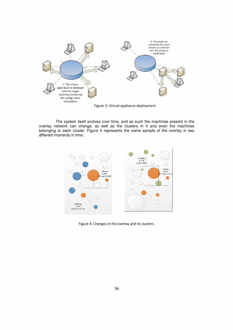
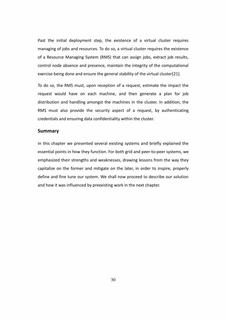
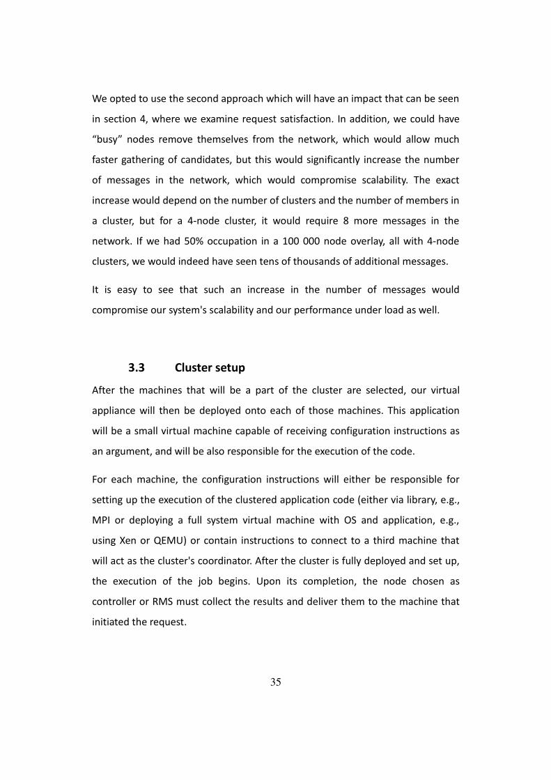
Figure 3: Virtual appliance deployment
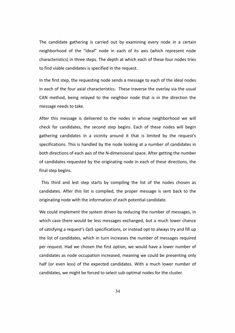
The system itself evolves over time, and as such the machines present in the overlay network can change, as well as the clusters in it and even the machines belonging to each cluster. Figure 4 represents the same sample of the overlay in two different moments in time.
Figure 4: Changes in the overlay and its clusters.
36

3.4 Further detail and Implementation Issues
To implement our resource discovery protocol we will address a number of
options that can be later compared regarding completeness, efficiency and
scalability. We can opt for a decentralized method with flooding via neighboring
nodes and random walks (Variant A), which is a method used in several existing
systems that use unstructured peer-to-peer overlays. This approach is both
simple and effective, but might not be the most efficient one.
Additionally we can use an approach similar to that of CAN (Variant B), where
resources are located by obtaining from the resource key its respective set of
coordinates in the N-Dimensional space. After obtaining the resource's
coordinates, getting to the resource is a question of forwarding the request to
the neighboring node that is in the direction of the set of coordinates.
This second approach will require a more strict placement of resources. In order
for the location to help us, we must have to set similar machines in similar
spaces, thus ensuring that should we require, for example, several machines with
3000 MHz of CPU, 2 GB of available RAM and low latency between them, we can
know where in the space to look.
In order to avoid two machines falling into the same space, there must be a
certain degree of leeway in the exact coordinates. Two machines with the exact
same components might end up at coordinates X,Y,Z and X+-α,Y+-β,Z+-γ. We will
now provide a simple depiction of the progress of the resource location protocol
in this approach.
37

Main steps in resource discovery
-Locate the coordinates of a resource from its characteristics and key;
-From the local node's coordinates, locate the neighboring node that lies in the
direction of the coordinates of the resource we obtained in the previous step;
- If the resource is located in that node's space, stop, if not, we locate the next
neighboring node that is in the direction of the coordinates;
- We then repeat the previous two steps
In Figure 5 we can see an example of the representation of a few nodes in a
coordinate system such as this one. For the sake of simplicity, we will only use
two dimensions, one for the number of cores and the other for each core's clock
speed, but any amount of characteristics can be presented in a N-dimensional
space.
The table below shows the characteristics of the nodes that will be present in
Figure 5.
38

Node Clock Speed
(MHz)
Number of
cores
Available
Bandwidth (Mb)
RAM
(MB)
Latency (ms)
1 2000 2 12 2000 55
2 2500 2 30 2000 43
3 3000 2 8 4000 118
4 3500 8 100 8000 45
5 3000 4 30 4000 61
Figure 5: Node representation in variant B
Each circle represents a node in this section of the overlay, and each node's
location in the 2-dimensional space tells us of the node's characteristics. By using
this information we can easily locate resources with specific characteristics.
A more advanced approach (Variant C) can extend the latter one, by using not
the exact position but the relative size of a resource in several 2-dimensional
planes. The more CPU a machine might have available, the larger the area it
occupies on that dimension in the coordinate space, and thus the higher chance
a random coordinate might fit it.
39
0 2 4 6 8 10 12 14 16
1500
2000
2500
3000
3500
4000
Number of cores
Clo
ck s
pe
ed
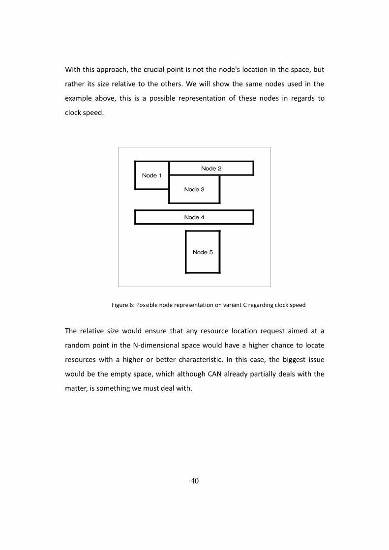
With this approach, the crucial point is not the node's location in the space, but
rather its size relative to the others. We will show the same nodes used in the
example above, this is a possible representation of these nodes in regards to
clock speed.
Figure 6: Possible node representation on variant C regarding clock speed
The relative size would ensure that any resource location request aimed at a
random point in the N-dimensional space would have a higher chance to locate
resources with a higher or better characteristic. In this case, the biggest issue
would be the empty space, which although CAN already partially deals with the
matter, is something we must deal with.
40
Node 1
Node 2
Node 3
Node 4
Node 5
In this approach, the location of a resource is, for each plane (we represent each
characteristic as a 2-dimensional axis), we create a random 2-dimension
coordinate. The machines with more processing power, or more bandwidth, or
more RAM, or less latency (size can in this case be inversely related to the latency
shown in the network) are more likely to be chosen than the others. This can
greatly accelerate resource location and maximize resource occupation in the
network.
Cluster Deployment
To facilitate cluster setup we will adhere to the Open Virtualization Format (OVF)
standard. This will allow us to utilize .OVA files that can be customized from
preexisting templates in order to allow us to refer our virtual appliance to
resources located on virtual disks containing the application to be executed.
These packages can be extended with configuration data to be accessed by the
virtual machine post-deployment.
Simulation
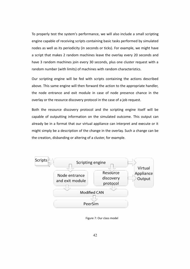
We will structure our system on top of PeerSim using classes developed to handle
node entrance and exit, as well as common resource discovery requests and job
execution requests (as depicted in Figure 7).
41
To properly test the system's performance, we will also include a small scripting
engine capable of receiving scripts containing basic tasks performed by simulated
nodes as well as its periodicity (in seconds or ticks). For example, we might have
a script that makes 2 random machines leave the overlay every 20 seconds and
have 3 random machines join every 30 seconds, plus one cluster request with a
random number (with limits) of machines with random characteristics.
Our scripting engine will be fed with scripts containing the actions described
above. This same engine will then forward the action to the appropriate handler,
the node entrance and exit module in case of node presence chance in the
overlay or the resource discovery protocol in the case of a job request.
Both the resource discovery protocol and the scripting engine itself will be
capable of outputting information on the simulated outcome. This output can
already be in a format that our virtual appliance can interpret and execute or it
might simply be a description of the change in the overlay. Such a change can be
the creation, disbanding or altering of a cluster, for example.
Figure 7: Our class model
42
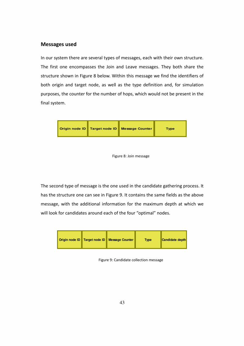
Messages used
In our system there are several types of messages, each with their own structure.
The first one encompasses the Join and Leave messages. They both share the
structure shown in Figure 8 below. Within this message we find the identifiers of
both origin and target node, as well as the type definition and, for simulation
purposes, the counter for the number of hops, which would not be present in the
final system.
Figure 8: Join message
The second type of message is the one used in the candidate gathering process. It
has the structure one can see in Figure 9. It contains the same fields as the above
message, with the additional information for the maximum depth at which we
will look for candidates around each of the four “optimal” nodes.
Figure 9: Candidate collection message
43
Origin node ID Target node ID Message Counter Type
Origin node ID Target node ID Message Counter Type Candidate depth
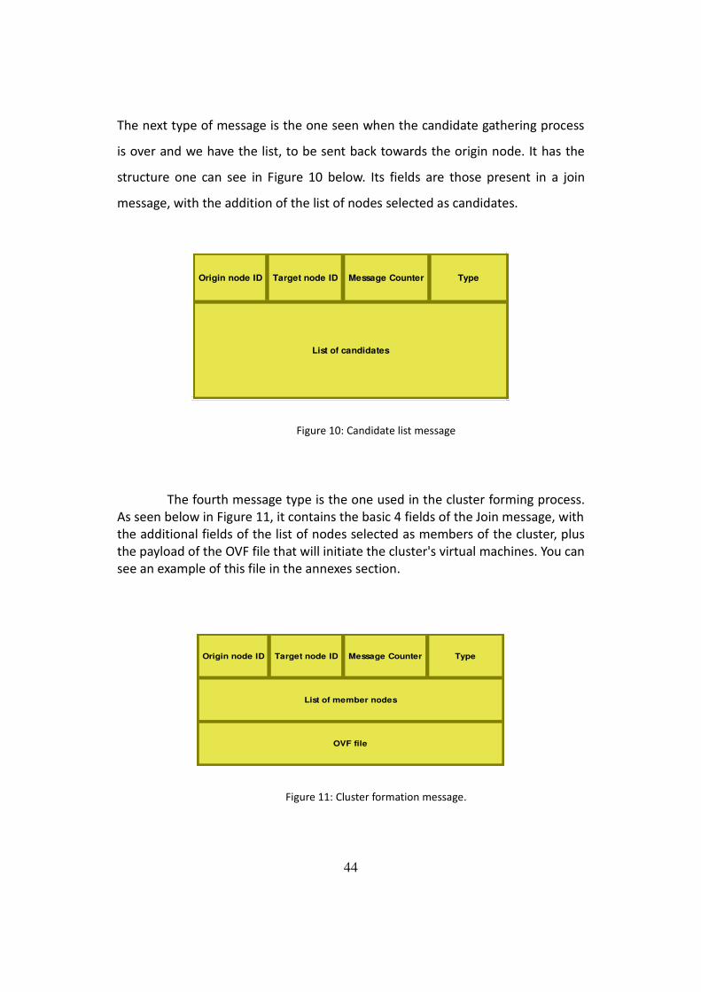
The next type of message is the one seen when the candidate gathering process
is over and we have the list, to be sent back towards the origin node. It has the
structure one can see in Figure 10 below. Its fields are those present in a join
message, with the addition of the list of nodes selected as candidates.
Figure 10: Candidate list message
The fourth message type is the one used in the cluster forming process.
As seen below in Figure 11, it contains the basic 4 fields of the Join message, with
the additional fields of the list of nodes selected as members of the cluster, plus
the payload of the OVF file that will initiate the cluster's virtual machines. You can
see an example of this file in the annexes section.
Figure 11: Cluster formation message.
44
Origin node ID Target node ID Message Counter Type
List of candidates
Origin node ID Target node ID Message Counter Type
List of member nodes
OVF file
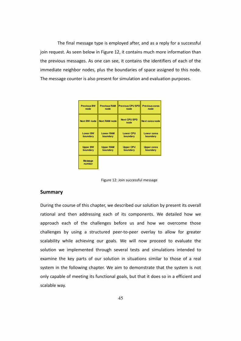
The final message type is employed after, and as a reply for a successful
join request. As seen below in Figure 12, it contains much more information than
the previous messages. As one can see, it contains the identifiers of each of the
immediate neighbor nodes, plus the boundaries of space assigned to this node.
The message counter is also present for simulation and evaluation purposes.
Figure 12: Join successful message
Summary
During the course of this chapter, we described our solution by present its overall
rational and then addressing each of its components. We detailed how we
approach each of the challenges before us and how we overcome those
challenges by using a structured peer-to-peer overlay to allow for greater
scalability while achieving our goals. We will now proceed to evaluate the
solution we implemented through several tests and simulations intended to
examine the key parts of our solution in situations similar to those of a real
system in the following chapter. We aim to demonstrate that the system is not
only capable of meeting its functional goals, but that it does so in a efficient and
scalable way.
45
Next BW node Next RAM node Next cores node
Previous BW
node
Previous RAM
node
Previous CPU SPD
node
Previous cores
node
Next CPU SPD
node
Lower BW
boundary
Lower RAM
boundary
Lower CPU
boundary
Lower cores
boundary
Upper BW boundary
Upper RAM boundary
Upper CPU boundary
Upper cores boundary
Message
number
4 Evaluation
To evaluate our application, we need to demonstrate that it correctly satisfies its
requirements, and in an efficient manner, both in terms of achieving its goals and
in doing it as effectively as possible.
We will begin by analyzing the system's behavior in simulated scenarios (as
realistically as possible in a large population) , and show that the results match
the expected outcome for the proposed architecture as a whole, as well as for
each of its components and message protocols.
4.1 Join and leave
First and foremost, we need to differentiate between behavior obtained in a
perfect network with stable machine presence and the behavior seen in a
network closer to the internet, where there is a large churn of machines both
leaving and joining the overlay.
In the first test, we measured the number of messages taken for any node to join
the network overlay when the number of nodes is maintained, for several sizes of
the overlay. As we can see in Figure 8, the distribution of message counts fits very
similar to a logarithmic expansion, which is coherent with the expected outcome
of Ω (n 1/d) where n is the number of nodes present in the overlay and d the
number of characteristic axis used, which in our case is 4. The leave process is
analogous to the join process. The node in question sends a message to a known
node, which then relays it to the neighbor nodes until it reaches the nodes that
will then be involved in the partition (or merge) action.
46

Each dot in Figure 13 below represents the result of a join request, with the
number of messages being displayed in the Y axis and the growing network
overlay size in the Y axis.
Figure 13: Number of messages taken for a Join message
X axis: Size of the network overlay, Y axis: Number of messages taken
For ease of comprehension, a line chart of the average number of messages sent
is also provided, wherein one can more easily notice the shape of the curve
47
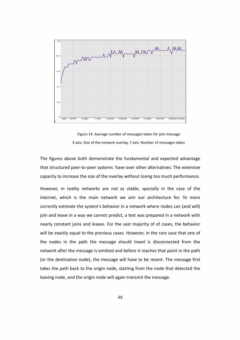
Figure 14: Average number of messages taken for join message
X axis: Size of the network overlay, Y axis: Number of messages taken
The figures above both demonstrate the fundamental and expected advantage
that structured peer-to-peer systems have over other alternatives: The extensive
capacity to increase the size of the overlay without losing too much performance.
However, in reality networks are not as stable, specially in the case of the
internet, which is the main network we aim our architecture for. To more
correctly estimate the system's behavior in a network where nodes can (and will)
join and leave in a way we cannot predict, a test was prepared in a network with
nearly constant joins and leaves. For the vast majority of of cases, the behavior
will be exactly equal to the previous cases. However, in the rare case that one of
the nodes in the path the message should travel is disconnected from the
network after the message is emitted and before it reaches that point in the path
(or the destination node), the message will have to be resent. The message first
takes the path back to the origin node, starting from the node that detected the
leaving node, and the origin node will again transmit the message.
48
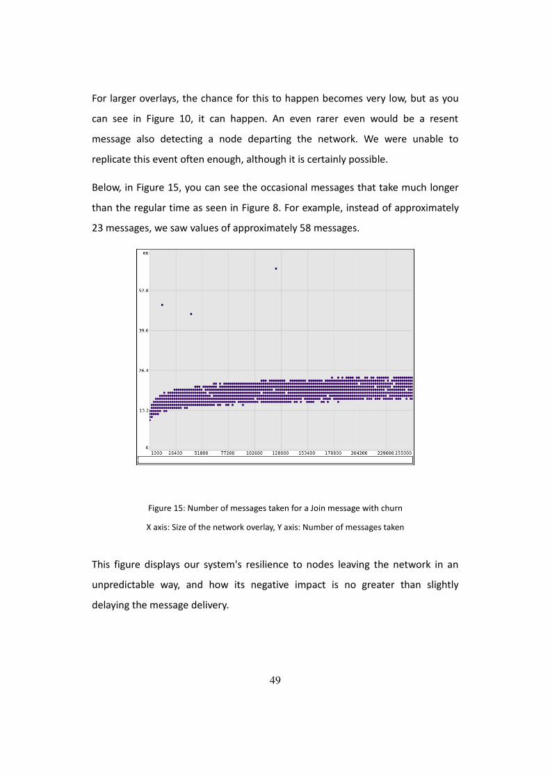
For larger overlays, the chance for this to happen becomes very low, but as you
can see in Figure 10, it can happen. An even rarer even would be a resent
message also detecting a node departing the network. We were unable to
replicate this event often enough, although it is certainly possible.
Below, in Figure 15, you can see the occasional messages that take much longer
than the regular time as seen in Figure 8. For example, instead of approximately
23 messages, we saw values of approximately 58 messages.
Figure 15: Number of messages taken for a Join message with churn
X axis: Size of the network overlay, Y axis: Number of messages taken
This figure displays our system's resilience to nodes leaving the network in an
unpredictable way, and how its negative impact is no greater than slightly
delaying the message delivery.
49
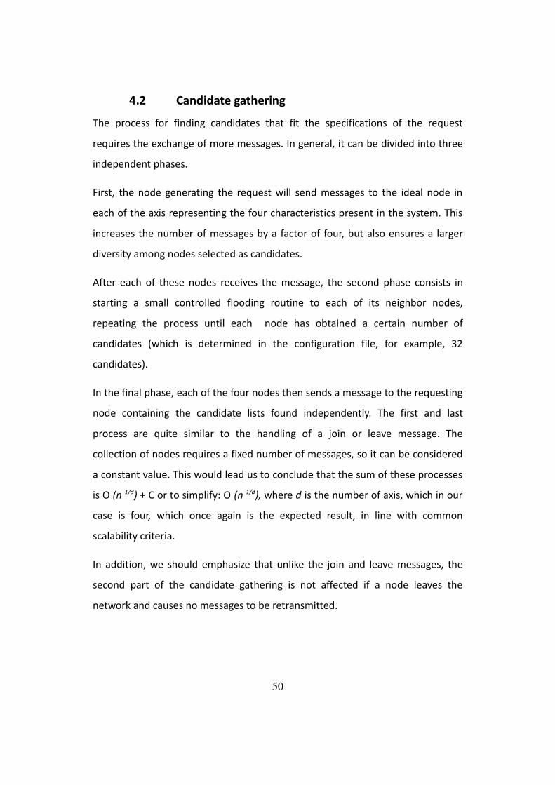
4.2 Candidate gathering
The process for finding candidates that fit the specifications of the request
requires the exchange of more messages. In general, it can be divided into three
independent phases.
First, the node generating the request will send messages to the ideal node in
each of the axis representing the four characteristics present in the system. This
increases the number of messages by a factor of four, but also ensures a larger
diversity among nodes selected as candidates.
After each of these nodes receives the message, the second phase consists in
starting a small controlled flooding routine to each of its neighbor nodes,
repeating the process until each node has obtained a certain number of
candidates (which is determined in the configuration file, for example, 32
candidates).
In the final phase, each of the four nodes then sends a message to the requesting
node containing the candidate lists found independently. The first and last
process are quite similar to the handling of a join or leave message. The
collection of nodes requires a fixed number of messages, so it can be considered
a constant value. This would lead us to conclude that the sum of these processes
is O (n 1/d) + C or to simplify: O (n 1/d), where d is the number of axis, which in our
case is four, which once again is the expected result, in line with common
scalability criteria.
In addition, we should emphasize that unlike the join and leave messages, the
second part of the candidate gathering is not affected if a node leaves the
network and causes no messages to be retransmitted.
50
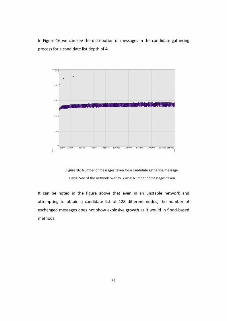
In Figure 16 we can see the distribution of messages in the candidate gathering
process for a candidate list depth of 4.
Figure 16: Number of messages taken for a candidate gathering message
X axis: Size of the network overlay, Y axis: Number of messages taken
It can be noted in the figure above that even in an unstable network and
attempting to obtain a candidate list of 128 different nodes, the number of
exchanged messages does not show explosive growth as it would in flood-based
methods.
51
4.3 Dynamic cluster forming
The final type of message interaction implemented by our architecture is the
cluster creation message which occurs after the nodes which will be part of the
virtual cluster (either as controller or regular cluster members). This message is
similar to a join or leave, but only slightly bigger in size. Since we are only
concerned with the number of messages exchanged for now, we will focus on
that aspect and examine each message's size in the following subsections.
Figure 17 displays the average number of messages required in the final phase to
establish a cluster. In this case, we used candidate depth = 4 and cluster size = 4
(3 slave + 1 controller).
Figure 17: Number of messages taken for a cluster forming message
X axis: Size of the network overlay, Y axis: Number of messages taken
52
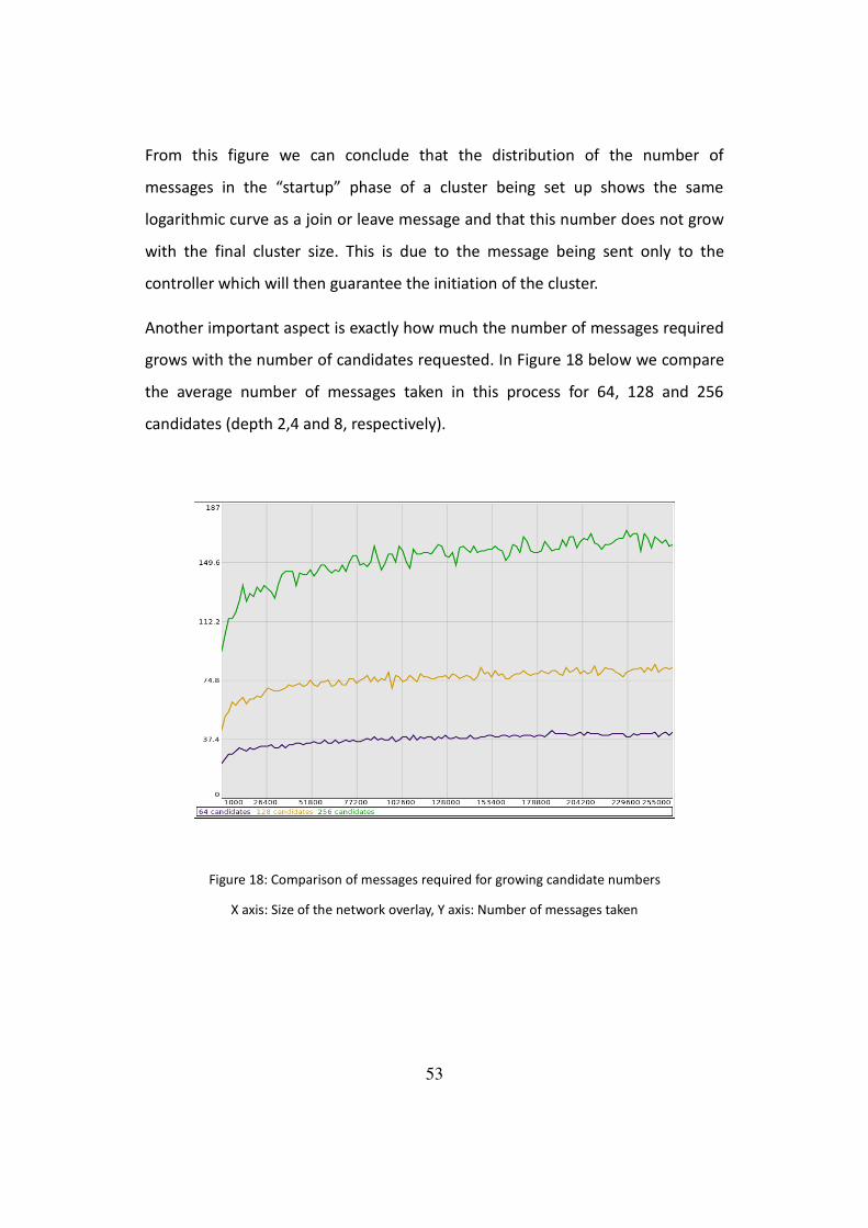
From this figure we can conclude that the distribution of the number of
messages in the “startup” phase of a cluster being set up shows the same
logarithmic curve as a join or leave message and that this number does not grow
with the final cluster size. This is due to the message being sent only to the
controller which will then guarantee the initiation of the cluster.
Another important aspect is exactly how much the number of messages required
grows with the number of candidates requested. In Figure 18 below we compare
the average number of messages taken in this process for 64, 128 and 256
candidates (depth 2,4 and 8, respectively).
Figure 18: Comparison of messages required for growing candidate numbers
X axis: Size of the network overlay, Y axis: Number of messages taken
53

We can see in this figure that the number of messages required for the gathering
of candidates grows with both the total size of the overlay as well as the number
of candidates we wish to gather for the final decision of which nodes will be
members of the cluster. Note that even at substantially high values such as 256
different candidates, the number of messages keeps its logarithmic properties,
hence supporting our claims of scalability.
4.4 Message size
However, there are more factors that can influence the viability of an application
in the real world. We have dealt with the number of messages, but we must also
focus on the size of each message, as well as the size of the information required
to store in, and about, each node, as well as to be exchanged, in order for the
system to work.
We will begin by examining the size each message occupies. The first type of
message is the one associated with the Join event. This message contains two
“int” type variables corresponding to the type of join and the counter of the
number of messages, as well as two 128-bit fields representing the identifier of
the target node and the origin node in addition to their axial coordinates.
Considering in the Java language an “int” occupies 32 bits, this means that a join
message will have 320 bits or 40 bytes of size. However, due to limitations on the
simulation tool we used (Peersim) the tests were performed with a variable of
type CANNode for target node and origin node.
54

This increases the size of a message in our tests to 672 bits or 84 bytes. We
should note that the counter for the number of messages is only necessary for
testing purposes, and could be omitted in the real system.
The leave message is the exact same as this one, and is subject to the same
limitations when it comes to Peersim.
The second type of message is the one related to the candidate gathering
process. This message contains all the fields in the join message and in addition
there is the presence of another “int” variable representing the intended depth
of the search. This increases the size to 352 bits or 44 bytes in the system/704
bits or 8 bytes in Peersim.
After the candidates are gathered, the message containing the found candidates
is sent back towards the origin node. This message contains the basic “join”
message and in addition it has an array of node identifiers wherein all candidates
are gathered. For a depth of 4, this would mean up to 128 additional positions in
the array with size equal to the identifiers for a total of 16704 bits or 2008 bytes.
We had the option of instead allowing each candidate to send a message back to
the originating node of the request, but the additional weight of the larger
amount of messages would imply more network occupation as well as higher
total size of messages. In taking this option over the alternative we took, we
would increase the chance to overload the network when multiple concurrent
requests are present.
The next message type is the one related to the process of actually establishing
the final virtual cluster. This message contains the same elements as a “join”
message and an array with the identifiers of each of the nodes selected to
become members of the virtual cluster as “slave” machines.
55
The message is sent to the node chosen as controller which will then relay the
message to the individual slaves. This message also contains the markup
language code relative to the startup of the virtual machine that will execute the
cluster code. This can be of variable size. An example can be found in the annexes
section.
The final message type is the one sent as acknowledgment to a join message.
This is much simpler and contains the neighboring nodes identifier, the “space”
that the origin node is assigned after joining and the message counter, for testing
purposes. This brings the total size of this message up to 352 bits or 44 bytes.
4.5 Size of the local data
We must also determine how much space is required of each node in order to
maintain the overlay's integrity and the system's functionality. With our
architecture, we require only that each node knows the location of each
neighboring node in each axis, plus the space the current node is assigned to
(possibly an extra neighbor in each direction to speed-up recovery when the
neighbor fails). This means a node needs a total of 8 ints (2 for each axis) and 8
CANNodes (again, 2 for each axis). This brings the total space assigned to
information about the overlay to 800 bits or 100 bytes.
Of course, in addition to this space, each node also needs to store its own
attributes in memory, which can be done with 4 more “int” variables, or 132 bits,
for a total of 932 bits or 117 bytes.
56
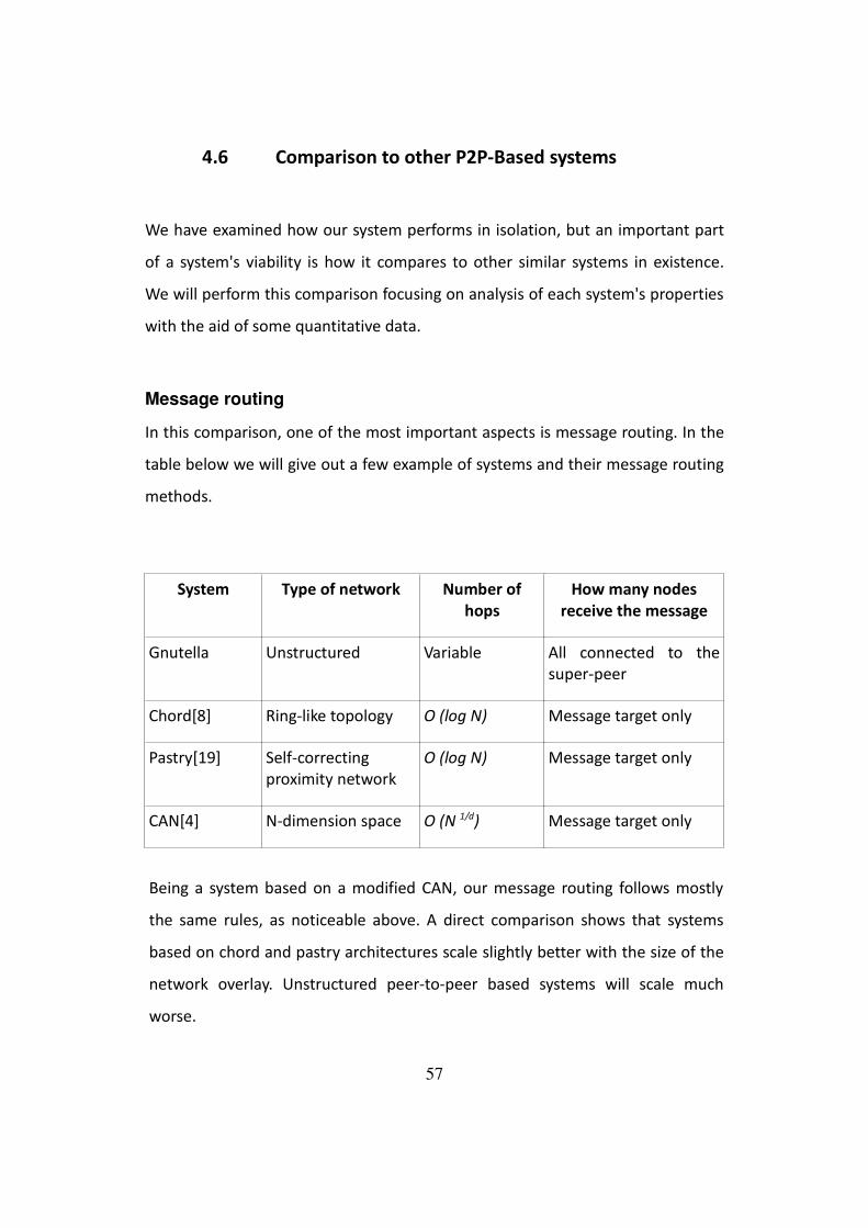
4.6 Comparison to other P2P-Based systems
We have examined how our system performs in isolation, but an important part
of a system's viability is how it compares to other similar systems in existence.
We will perform this comparison focusing on analysis of each system's properties
with the aid of some quantitative data.
Message routing
In this comparison, one of the most important aspects is message routing. In the
table below we will give out a few example of systems and their message routing
methods.
System Type of network Number of
hops
How many nodes
receive the message
Gnutella Unstructured Variable All connected to the
super-peer
Chord[8] Ring-like topology O (log N) Message target only
Pastry[19] Self-correcting
proximity network
O (log N) Message target only
CAN[4] N-dimension space O (N 1/d) Message target only
Being a system based on a modified CAN, our message routing follows mostly
the same rules, as noticeable above. A direct comparison shows that systems
based on chord and pastry architectures scale slightly better with the size of the
network overlay. Unstructured peer-to-peer based systems will scale much
worse.
57
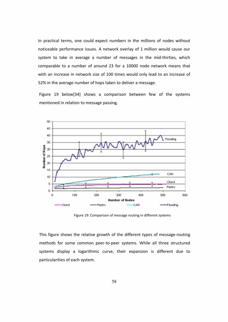
In practical terms, one could expect numbers in the millions of nodes without
noticeable performance issues. A network overlay of 1 million would cause our
system to take in average a number of messages in the mid-thirties, which
comparable to a number of around 23 for a 10000 node network means that
with an increase in network size of 100 times would only lead to an increase of
52% in the average number of hops taken to deliver a message.
Figure 19 below[34] shows a comparison between few of the systems
mentioned in relation to message passing.
Figure 19: Comparison of message routing in different systems
This figure shows the relative growth of the different types of message-routing
methods for some common peer-to-peer systems. While all three structured
systems display a logarithmic curve, their expansion is different due to
particularities of each system.
58
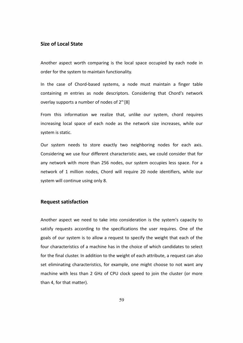
Size of Local State
Another aspect worth comparing is the local space occupied by each node in
order for the system to maintain functionality.
In the case of Chord-based systems, a node must maintain a finger table
containing m entries as node descriptors. Considering that Chord's network
overlay supports a number of nodes of 2m.[8]
From this information we realize that, unlike our system, chord requires
increasing local space of each node as the network size increases, while our
system is static.
Our system needs to store exactly two neighboring nodes for each axis.
Considering we use four different characteristic axes, we could consider that for
any network with more than 256 nodes, our system occupies less space. For a
network of 1 million nodes, Chord will require 20 node identifiers, while our
system will continue using only 8.
Request satisfaction
Another aspect we need to take into consideration is the system's capacity to
satisfy requests according to the specifications the user requires. One of the
goals of our system is to allow a request to specify the weight that each of the
four characteristics of a machine has in the choice of which candidates to select
for the final cluster. In addition to the weight of each attribute, a request can also
set eliminating characteristics, for example, one might choose to not want any
machine with less than 2 GHz of CPU clock speed to join the cluster (or more
than 4, for that matter).
59

Our system sorts the list of candidates according to each node's overall score,
eliminating any that do not fulfill the specific requirements. It then proceeds to
select as many nodes as required by the request in order from the sorted list.
This process of sorting is done using an algorithm with degree of complexity of Ω
n (log n). For a typical candidate depth of 4 (as used in our tests), this would
generate a candidate list of 128 different nodes (if this many nodes are available
in the overlay in the vicinity of the nodes controlling the space where the
request's ideal candidate exists).
In order to quantify the system's actual performance, it is important to determine
the percentage of requests that was satisfied either fully, partially or not satisfied
at all. To do so, we first created a standard distribution of nodes in our overlay
using commonly found machines. The table below explains the chance of each
node being created, for a grand total of 100 000 nodes.
Description Probability
4-core 3GHz 8 GB RAM 100 MBps 30,00%
2-core 2.5GHz 6 GB RAM 50 MBps 30,00%
2-core 2GHz 4 GB RAM 30 MBps 20,00%
Single-core 2GHz 2 GB RAM 6MBps 20,00%
We then proceeded to test the system above with a request for 4 2-core CPUs
with 2.5 GHz and 8 GB RAM (leaving network speed unchecked), and for all tests
wherein node occupation was below 60% we noticed that the requests were
satisfying 100% of the QoS metrics and only then did request satisfaction rate
started slowly dropping. You can see this in Figure 20 below.
60
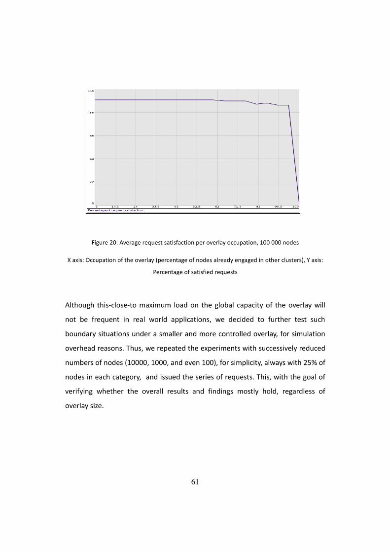
Figure 20: Average request satisfaction per overlay occupation, 100 000 nodes
X axis: Occupation of the overlay (percentage of nodes already engaged in other clusters), Y axis:
Percentage of satisfied requests
Although this-close-to maximum load on the global capacity of the overlay will
not be frequent in real world applications, we decided to further test such
boundary situations under a smaller and more controlled overlay, for simulation
overhead reasons. Thus, we repeated the experiments with successively reduced
numbers of nodes (10000, 1000, and even 100), for simplicity, always with 25% of
nodes in each category, and issued the series of requests. This, with the goal of
verifying whether the overall results and findings mostly hold, regardless of
overlay size.
61
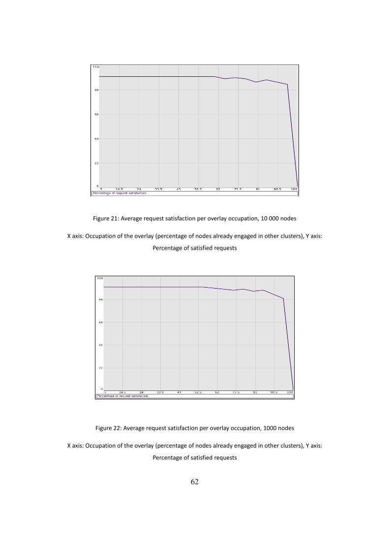
Figure 21: Average request satisfaction per overlay occupation, 10 000 nodes
X axis: Occupation of the overlay (percentage of nodes already engaged in other clusters), Y axis:
Percentage of satisfied requests
Figure 22: Average request satisfaction per overlay occupation, 1000 nodes
X axis: Occupation of the overlay (percentage of nodes already engaged in other clusters), Y axis:
Percentage of satisfied requests
62
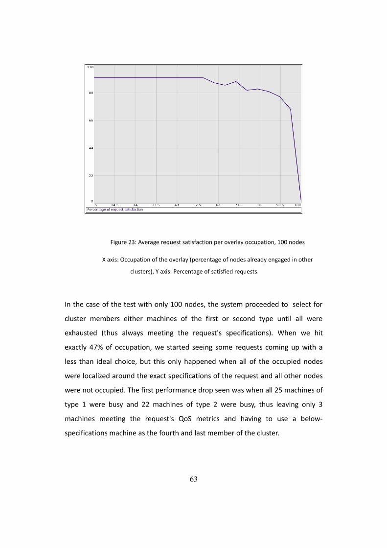
Figure 23: Average request satisfaction per overlay occupation, 100 nodes
X axis: Occupation of the overlay (percentage of nodes already engaged in other
clusters), Y axis: Percentage of satisfied requests
In the case of the test with only 100 nodes, the system proceeded to select for
cluster members either machines of the first or second type until all were
exhausted (thus always meeting the request's specifications). When we hit
exactly 47% of occupation, we started seeing some requests coming up with a
less than ideal choice, but this only happened when all of the occupied nodes
were localized around the exact specifications of the request and all other nodes
were not occupied. The first performance drop seen was when all 25 machines of
type 1 were busy and 22 machines of type 2 were busy, thus leaving only 3
machines meeting the request's QoS metrics and having to use a below-
specifications machine as the fourth and last member of the cluster.
63
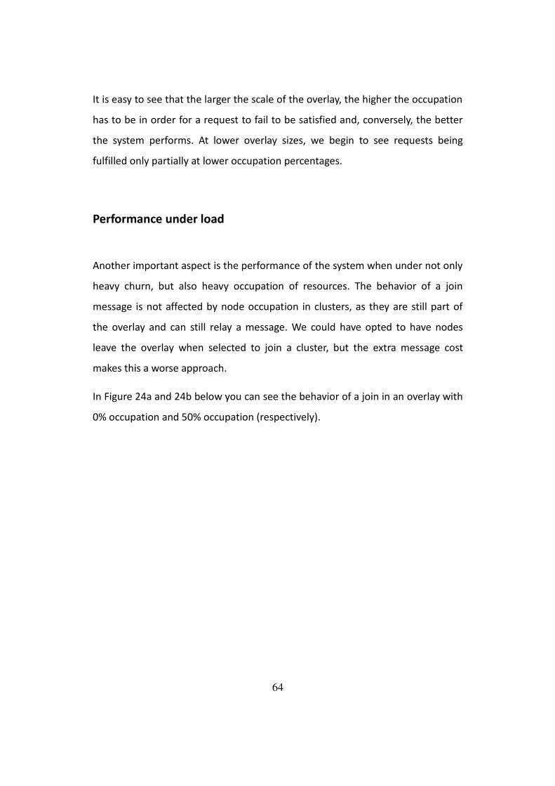
It is easy to see that the larger the scale of the overlay, the higher the occupation
has to be in order for a request to fail to be satisfied and, conversely, the better
the system performs. At lower overlay sizes, we begin to see requests being
fulfilled only partially at lower occupation percentages.
Performance under load
Another important aspect is the performance of the system when under not only
heavy churn, but also heavy occupation of resources. The behavior of a join
message is not affected by node occupation in clusters, as they are still part of
the overlay and can still relay a message. We could have opted to have nodes
leave the overlay when selected to join a cluster, but the extra message cost
makes this a worse approach.
In Figure 24a and 24b below you can see the behavior of a join in an overlay with
0% occupation and 50% occupation (respectively).
64
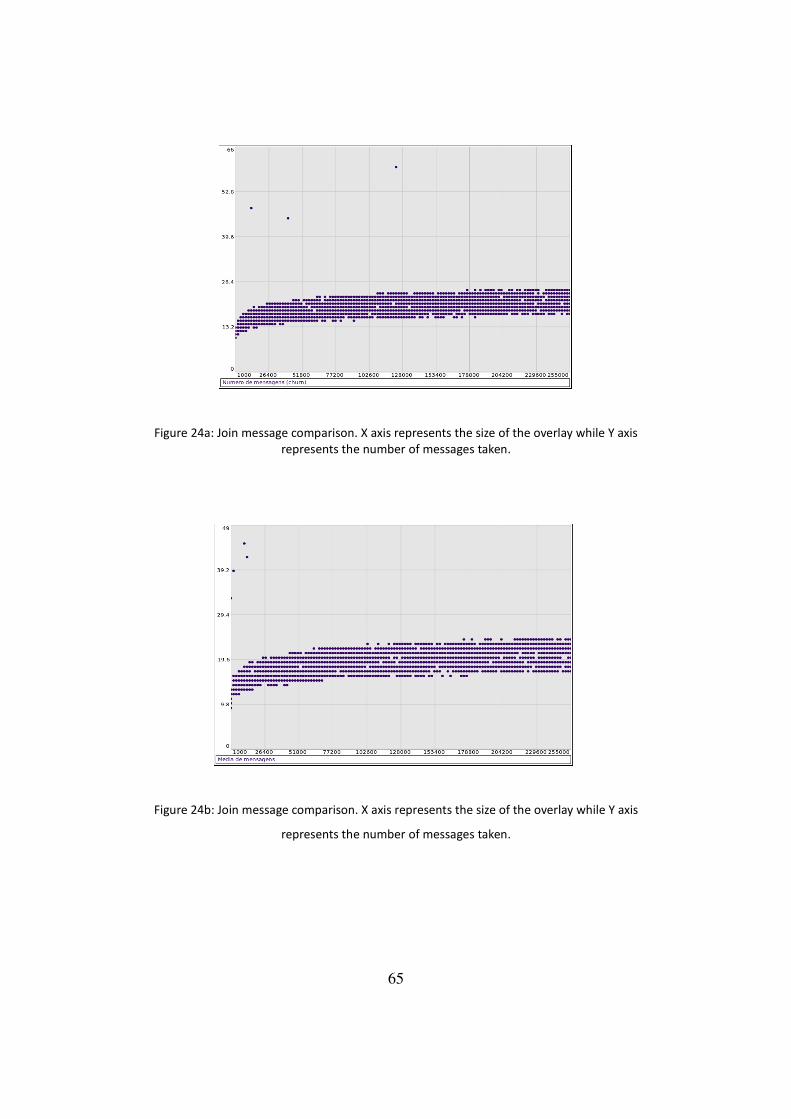
Figure 24a: Join message comparison. X axis represents the size of the overlay while Y axis
represents the number of messages taken.
Figure 24b: Join message comparison. X axis represents the size of the overlay while Y axis
represents the number of messages taken.
65
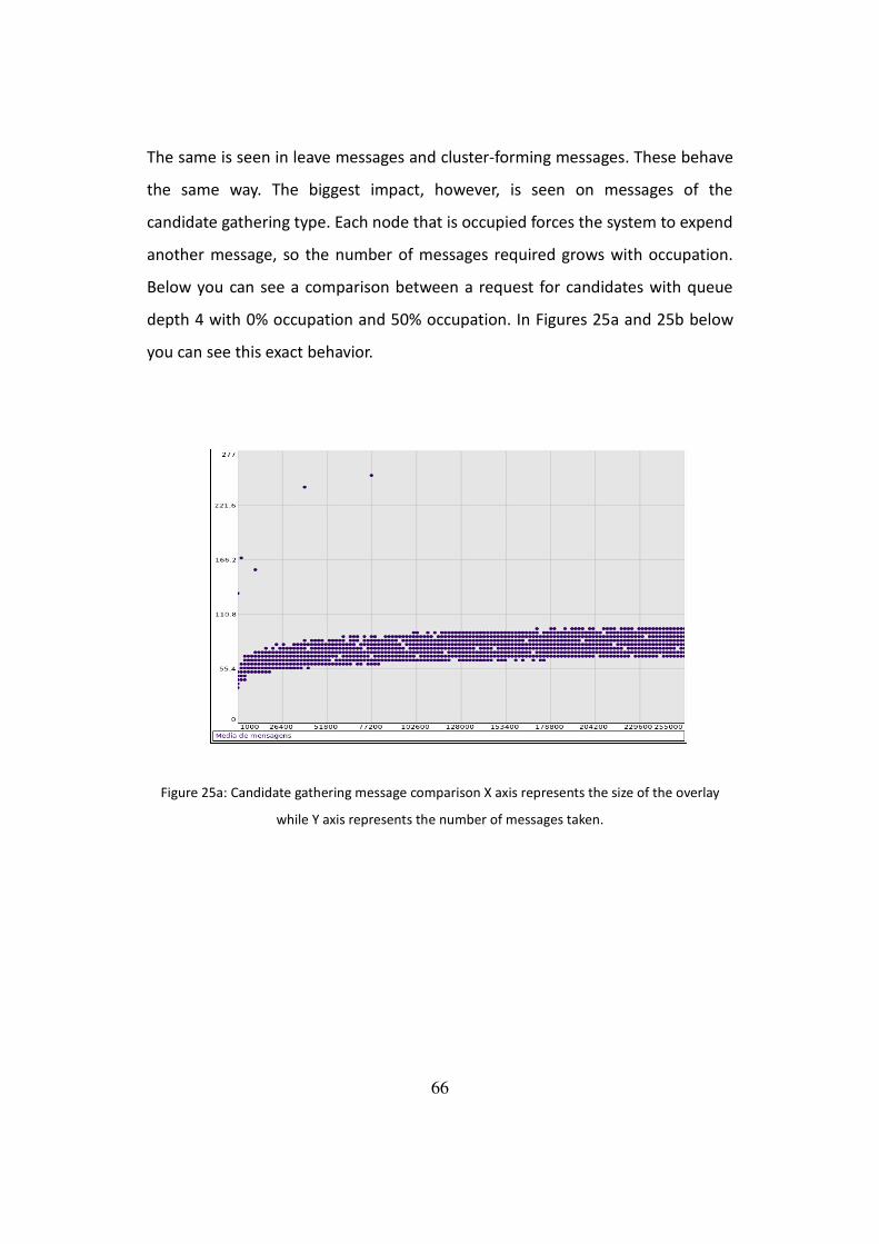
The same is seen in leave messages and cluster-forming messages. These behave
the same way. The biggest impact, however, is seen on messages of the
candidate gathering type. Each node that is occupied forces the system to expend
another message, so the number of messages required grows with occupation.
Below you can see a comparison between a request for candidates with queue
depth 4 with 0% occupation and 50% occupation. In Figures 25a and 25b below
you can see this exact behavior.
Figure 25a: Candidate gathering message comparison X axis represents the size of the overlay
while Y axis represents the number of messages taken.
66
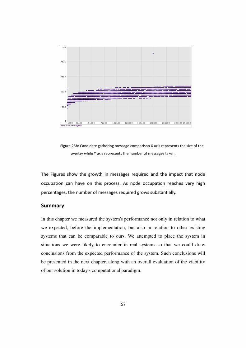
Figure 25b: Candidate gathering message comparison X axis represents the size of the
overlay while Y axis represents the number of messages taken.
The Figures show the growth in messages required and the impact that node
occupation can have on this process. As node occupation reaches very high
percentages, the number of messages required grows substantially.
Summary
In this chapter we measured the system's performance not only in relation to what
we expected, before the implementation, but also in relation to other existing
systems that can be comparable to ours. We attempted to place the system in
situations we were likely to encounter in real systems so that we could draw
conclusions from the expected performance of the system. Such conclusions will
be presented in the next chapter, along with an overall evaluation of the viability
of our solution in today's computational paradigm.
67

5 Conclusion
The amount of computational resources worldwide that sit idle for lengthy
periods of time while connected to a network is immense. By utilizing these
untapped resources we could harness a massive amount of computational power.
The increasing complexity of applications and computations required by the
typical home-user is growing and by providing such users with the means to
access computational power that typically was only accessible to large-scale
companies allows him to better and faster perform everyday computational
tasks, which is particularly useful for the most time-consuming ones.
The great obstacles to such an outcome are the lack of systems and architectures
capable of not only allowing local resources to be available to others, but also to
properly utilize remote resources and shape them into organized clusters capable
of adapting to the characteristics of the application to be executed.
We present in this thesis a system that can overcome such obstacles, a system
capable of efficiently locating remote resources, setup specialized clusters and
allow a high degree of control to the user, in the form of quality-of-service
metrics that specify in fine-grain exactly the characteristics that such a cluster
needs to best fit the application being ran. This system performs this in over a
peer-to-peer overlay of nodes in order to allow for greater scalability with a
growing number of nodes, as well as faster resource discovery.
Our evaluation methods, to which we subjected the system and architecture,
measured its performance both in isolation as well as when compared to other
systems.
68
We began by testing the number of messages taken by the system and how it
was affected by the size of the network overlay. As expected, even though the
number of messages required for each of the phases of request handling grew
with the overlay size, its growth was much slower than the growth of the
network itself. In fact, at 250 000 nodes in the network, we were seeing around
25 messages for a typical message routing from one node to another, meaning
0.01% of the size. As the number of nodes in the overlay increases, we will notice
even higher efficiency by our system. This indeed demonstrates that our system
can scale very efficiently with the overlay size, which is one of the main
requirements and expectations we had about the system.
We proceeded to examine the size of each message used in our system. Most of
the messages have a very small size, below 100 bytes, which implies that the
overall traffic in the overlay will not be significantly increased by the functioning
of the system. The exception, the message sent when the list of candidates is
completed, is substantially bigger, but still acceptable, and of course, the smaller
the number of candidates obtained, the smaller the message. We could have
opted for using multiple messages (one per candidate), which would greatly
reduce the size of the message, but it would multiply the number of required
messages by a large number and aggravate latency.
Having chosen one larger message, we ensure that we maintain a small number
of messages required for each request, also increasing our scalability by
diminishing the chance we will flood the bandwidth of the nodes in the overlay.
In addition, by choosing to obtain candidates around 4 different nodes instead of
only the ideal node, we increase the chance that different nodes will be chosen
as candidates for each request, as well as allow a small degree of parallelism that
speeds up the process slightly.
69

We then focused on the local storage size each node requires to maintain the
system's effectiveness. The local size, while for a smaller number of nodes
present in the overlay is slightly bigger than the space required for systems like
Chord or Pastry, does not grow significantly at all with the number of nodes in
the overlay, which is a substantial advantage over other systems. For very large
number of nodes in the overlay, our system occupies significantly less space.
While in fact local storage space has lowered in cost, it is still an advantage that
should not be ignored.
We also examined how our system would perform under higher overlay node
occupation numbers, to certify that our solution performs as expected even in
extreme situations that we could encounter in a real scenario. Even with very
high overlay occupation, our system scales very well, and only the node
gathering is substantially impacted.
All four points above could be considered essential for any system to be
considered viable and worthy of deploying after implementation. We ensured
that our system is up to the task with several evaluation measures that proved
how well the protocol performs, both in scalability, speed and effectiveness in
handling resources. We believe the architecture shown in this paper is thus
capable of providing a much needed tool to a substantial niche in today's
computer user world, furthering the state of the art in public distributed
computing and contributing to fulfill the basic two goals we set forth to reach: i)
providing common users with computational power far beyond what was
available in the past, and ii) efficiently managing resources in such a way as to
diminish resource wasting in today's interconnected world.
70
Future Work
However, the work in this larger scope project is far from finished. Several
aspects are worth additional research into optimization and some aspects require
an extra investment of time into design refinements:
• The messages exchanged are currently sent unencrypted and without any
form of security, be it authentication or certification of origin or validity.
• Peersim, while a handy tool for simulating a peer-to-peer overlay, cannot
effectively represent a real scenario, and lacks the robustness to handle
numbers of nodes into the high millions. Therefore a real deployment on
testbeds or even with voluntary users could result in more relevant data
concerning user's habits.
• Variation C of the overlay setup described in chapter 3 also merits further
investigation, but it would imply a more hierarchical overlay structure. It
would require certain nodes to behave as super-peers, which could only
apply in the case of either network service providers or maybe academic
labs or other large installations of PCs delivering the machines that would
perform this role.
In addition, for production purposes, a substantial degree of optimization and
testing should be undertaken in order to ensure the perfect performance of the
system.
71
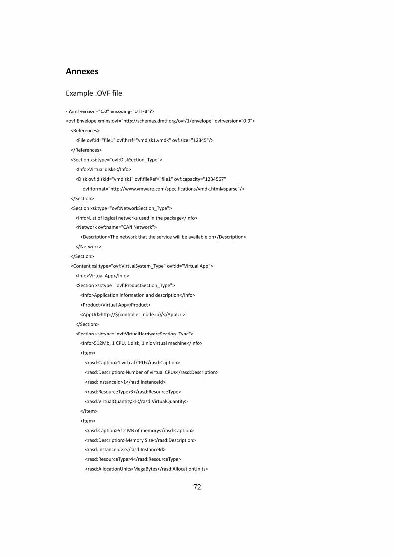
Annexes
Example .OVF file
<?xml version="1.0" encoding="UTF-8"?>
<ovf:Envelope xmlns:ovf="http://schemas.dmtf.org/ovf/1/envelope" ovf:version="0.9">
<References>
<File ovf:id="file1" ovf:href="vmdisk1.vmdk" ovf:size="12345"/>
</References>
<Section xsi:type="ovf:DiskSection_Type">
<Info>Virtual disks</Info>
<Disk ovf:diskId="vmdisk1" ovf:fileRef="file1" ovf:capacity="1234567"
ovf:format="http://www.vmware.com/specifications/vmdk.html#sparse"/>
</Section>
<Section xsi:type="ovf:NetworkSection_Type">
<Info>List of logical networks used in the package</Info>
<Network ovf:name="CAN Network">
<Description>The network that the service will be available on</Description>
</Network>
</Section>
<Content xsi:type="ovf:VirtualSystem_Type" ovf:id="Virtual App">
<Info>Virtual App</Info>
<Section xsi:type="ovf:ProductSection_Type">
<Info>Application information and description</Info>
<Product>Virtual App</Product>
<AppUrl>http://${controller_node.ip}/</AppUrl>
</Section>
<Section xsi:type="ovf:VirtualHardwareSection_Type">
<Info>512Mb, 1 CPU, 1 disk, 1 nic virtual machine</Info>
<Item>
<rasd:Caption>1 virtual CPU</rasd:Caption>
<rasd:Description>Number of virtual CPUs</rasd:Description>
<rasd:InstanceId>1</rasd:InstanceId>
<rasd:ResourceType>3</rasd:ResourceType>
<rasd:VirtualQuantity>1</rasd:VirtualQuantity>
</Item>
<Item>
<rasd:Caption>512 MB of memory</rasd:Caption>
<rasd:Description>Memory Size</rasd:Description>
<rasd:InstanceId>2</rasd:InstanceId>
<rasd:ResourceType>4</rasd:ResourceType>
<rasd:AllocationUnits>MegaBytes</rasd:AllocationUnits>
72
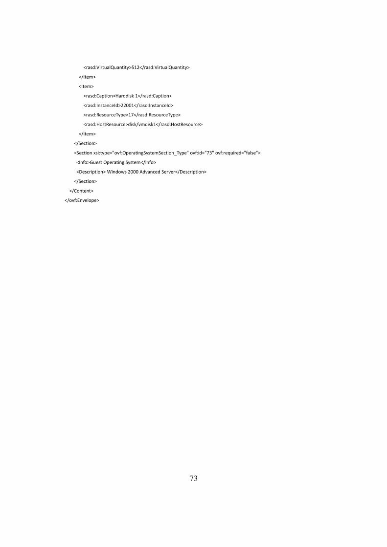
<rasd:VirtualQuantity>512</rasd:VirtualQuantity>
</Item>
<Item>
<rasd:Caption>Harddisk 1</rasd:Caption>
<rasd:InstanceId>22001</rasd:InstanceId>
<rasd:ResourceType>17</rasd:ResourceType>
<rasd:HostResource>disk/vmdisk1</rasd:HostResource>
</Item>
</Section>
<Section xsi:type="ovf:OperatingSystemSection_Type" ovf:id="73" ovf:required="false">
<Info>Guest Operating System</Info>
<Description> Windows 2000 Advanced Server</Description>
</Section>
</Content>
</ovf:Envelope>
73
Bibliography
1: Schollmeier, R, A Definition of Peer-to-Peer Networking for the Classification of Peer-to-Peer
Architectures and Applications, 2002, Proceedings. First International Conference on Peer-to-Peer
Computing, 2001. IEEE
2: Foster, I; Kesselman, C; Lee, C; Lindell, B; Nahrstedt, K; Roy, A, A distributed resource
management architecture that supports advance reservations and co-allocation, 2002, 1999
Seventh International Workshop on Quality of Service, 1999. IWQoS'99
3: Buyya, R; Venugopal, S, A Gentle Introduction toGrid Computing and Technologies, 2005
4: S. Ratnasamy, P. Francis, M. Handley, R. Karp, and S. Schenker, A scalable content-addressable
network, 2001, Proceedings of the 2001 conference on Applications, technologies, architectures,
and protocols for computer communications, ACM
5: Ghosemajumder, S, Advanced Peer-Based Technology Business Models, 2002, MIT Sloan School
of Management, Citeseer,
6: Jon Brodkin, Case Study: Parallel Internet: Inside the Worldwide LHC computing Grid, 2008,
Techworld
7: A.; Karaul, M., Kedem, Z., Wyckoff, P, Charlotte: Metacomputing on the Web, 1996, 9th
International Conference on Parallel and Distributed Computing Systems
8: I Stoica, R Morris, D Karger, and M Kaashoek, Chord: A scalable peer-to-peer lookup service for
internet applications, 2001, Proceedings of the 2001 conference on Applications, technologies,
architectures, and protocols for computer communications, ACM
9: STIMI, K.O., CLUSTER COMPUTING, 2008, COCHIN UNIVERSITY OF SCIENCE AND TECHNOLOGY
10: Thain, D; Tannenbaum, T; Livny, M, Distributed Computing in Practice: the Condor Experience,
2005, University of Wisconsin
11: Ghodsi, A, Distributed k-ary System: Algorithms for Distributed Hash Tables, 2006, KTH-Royal
Institute of Technology
12: Veiga, L; Rodrigues, R; Ferreira, P, Gigi: An ocean of gridlets on a ”grid-for-the-masses”, 2007,
Cluster Computing and the Grid, 2007. CCGRID 2007. Seventh IEEE International Symposium on
13: Foster, I; Kesselman, C, Globus: A metacomputing infrastructure toolkit, 1997, International
Journal of High Performance Computing Applications, SAGE Publications
14: %A Loguinov, D; Kumar, A; Rai, V; Ganesh, S, Graph-theoretic analysis of structured peer-to-
peer systems: routing distances and fault resilience, 2003, Proceedings of the 2003 conference on
Applications, technologies, architectures, and protocols for computer communications, ACM
15: ED2K, http://kent.dl.sourceforge.net/pdonkey/eDonkey-protocol-0.6.2.html eDonkey protocol
documentation, ,
16: P. Maymounkov; D. Mazières, Kademlia: A peer-to-peer informationsystem based on the xor
metric, 2002, IPTPS02 Peer-to-Peer Systems, Springer
17: Balakrishnan, H; Kaashoek, MF; Karger, D; Morris, R; Stoica, I, Looking up data in P2P systems,
2003, Communications of the ACM
74
18: Foster, I; Iamnitchi, A, On Death, Taxes, and the Convergence of Peer-to-Peer and Grid
Computing, 2003, University of Chicago
19: Rowstron, A; Druschel, P, Pastry: Scalable, decentralized object location and routing for large-
scale peer-to-peer systems., 2001, Microsoft Research LTD
20: %A Gkantsidis, C; Mihail, M; Saberi, A, Random walks in peer-to-peer networks: algorithms
and evaluation, 2006, Georgia Institute of Technology
21: Begnum, KM; Disney, M, Scalable deployment and configuration of high-performance virtual
clusters, 2005, International Journal of Applied Mathematics and Computer Sciences, Citeseer
22: Silva, JN; Ferreira, P; Veiga, L, Service and resource discovery in cycle-sharing environments
with a utility algebra, 2010, 2010 IEEE International Symposium on Parallel & Distributed
Processing (IPDPS), IEEE
23: Tamilmani, K, Studying and enhancing the BitTorrent protocol, 2003, Stony Brook University
24: Nakada, H; Yokoi, T; Ebara, T; Tanimura, Y; Ogawa, H; Sekiguchi, S, The design and
implementation of a virtual cluster management system, 2007, Proceedings of the first IEEE/IFIP
International Workshop on End-to-end Virtualization and Grid Management (EVGM2007)
25: Foster, I; Kesselman, C, The Grid: Blueprint for a New Computing Infrastructure, 1999, Morgan
Kaufmann Publishers
26: Nisan, N, The POPCORN Market – an Online Market for ComputationalResources, 1998,
27: Carlsson, B; Gustavsson, R, The Rise and Fall of Napster - An Evolutionary Approach, 2001, 6th
International Computer Science Conference on Active Media Technology, Springer
28: Gropp, W; Thakur, R; Lusk, E, Using MPI-2: Advanced Features of the Message Passing
Interface, 1999, MIT Press, 0-262-57133-1
29: Gropp, W; Lusk, E; Skjellum, A, Using MPI: Portable Parallel Programming with the Message-
Passing Interface, 1994, MIT Press, 0-262-57104-8
30: Nishimura, H; Maruyama, N; Matsuoka, S, Virtual clusters on the fly-fast, scalable, and flexible
installation, 2007, IEEE Computer Society
31: Keahey, K; Foster, I; Freeman, T; Zhang, X; Galron, D, Virtual workspaces in the grid, 2005,
Euro-Par 2005 Parallel Processing
32: Krsul, I; Ganguly, A; Zhang, J; Fortes, JAB; Figueiredo, RJ, Vmplants: Providing and managing
virtual machine execution environments for grid computing, 2005, Supercomputing, 2004.
Proceedings of the ACM/IEEE SC2004 Conference
33: Foster, I, What is the Grid? A Three Point Checklist, 2002, University of Chicago
34: M. Kelaskar , V. Matossian, P. Mehra, D. Paul, and M. Parashar, A Study of Discovery
Mechanisms for Peer-to-Peer Applications, 2002, Department of Electrical and Computer
Engineering, Rutgers University, Piscataway, NJ
75