RESOURCE MANAGEMENT IN CLUSTER COMPUTINGPLATFORMS FOR LARGE SCALE DATA PROCESSING

A Dissertation Presented

By

Yi Yao

to

The Department of Electrical and Computer Engineering

in partial fulfillment of the requirements

for the degree of

Doctor of Philosophy

in the field of

Computer Engineering

Northeastern University

Boston, Massachusetts

August, 2015

Acknowledgement

I would like to express my very great appreciation to the following people. This

dissertation would not have been possible without the support of them. Many thanks

to my adviser Professor Ningfang Mi for the continuous guidance of my PhD, for

her patience, motivation, and immense knowledge. The work in this dissertation is

the result of collaboration with many other people. I wish to acknowledge the help

provided by Professor Bo Sheng, Jiayin Wang, Jianzhe Tai, Jason Lin, and Chiu Tan.

I would like to offer my special thanks to my thesis committee members, Professor

Mirek Riedewald, Doctor Xiaoyun Zhu, and Professor Yunsi Fei. Thank you very

much for your helpful feedback. I thank my fellow labmates for the discussions,

working together, and for all the fun we have had in the last five years. Last but

not least, I am particularly grateful for the unwavering support from my family and

friends through my PhD.

To my family

iv

Contents

Contents iv

Abstract . . . . . . . . . . . . . . . . . . . . . . . . . . . . . . . . . . . vi

1 Introduction 1

1.1 Features of Cluster Computing Platforms and Applications . . . . . . 3

1.2 Summary of Contributions . . . . . . . . . . . . . . . . . . . . . . . . . 6

1.3 Dissertation Outline . . . . . . . . . . . . . . . . . . . . . . . . . . . . 7

2 Background 9

2.1 MapReduce Programming Paradigm . . . . . . . . . . . . . . . . . . . 9

2.2 Hadoop MapReduce . . . . . . . . . . . . . . . . . . . . . . . . . . . . 10

2.3 Hadoop YARN . . . . . . . . . . . . . . . . . . . . . . . . . . . . . . . 11

2.4 Scheduling Policies . . . . . . . . . . . . . . . . . . . . . . . . . . . . . 12

3 Resource Management for Hadoop MapReduce 14

3.1 A Job Size-Based Scheduler for Hadoop MapReduce . . . . . . . . . . 15

3.1.1 Motivation . . . . . . . . . . . . . . . . . . . . . . . . . . . . . 15

3.1.2 Algorithm Description . . . . . . . . . . . . . . . . . . . . . . . 19

3.1.3 Model Description . . . . . . . . . . . . . . . . . . . . . . . . . 26

3.1.4 Evaluation . . . . . . . . . . . . . . . . . . . . . . . . . . . . . 27

3.2 Self-Adjusting Slot Configurations for Hadoop MapReduce . . . . . . . 40

3.2.1 Motivation . . . . . . . . . . . . . . . . . . . . . . . . . . . . . 41

3.2.2 System Model and Static Slot Configuration . . . . . . . . . . . 44

3.2.3 Dynamic Slot Configuration Under Homogeneous Environments 46

3.2.4 Dynamic Slot Configuration Under Heterogeneous Environments 52

v

3.2.5 Evaluation . . . . . . . . . . . . . . . . . . . . . . . . . . . . . 56

3.3 Related Work . . . . . . . . . . . . . . . . . . . . . . . . . . . . . . . . 67

3.4 Summary . . . . . . . . . . . . . . . . . . . . . . . . . . . . . . . . . . 69

4 Resource Management for Hadoop YARN 70

4.1 Scheduling for YARN MapReduce . . . . . . . . . . . . . . . . . . . . 72

4.1.1 Problem Formulation . . . . . . . . . . . . . . . . . . . . . . . 73

4.1.2 Sketch of HaSTE Design . . . . . . . . . . . . . . . . . . . . . . 75

4.1.3 Initial Task Assignment . . . . . . . . . . . . . . . . . . . . . . 75

4.1.4 Real-time Task Assignment . . . . . . . . . . . . . . . . . . . . 77

4.1.5 Evaluation . . . . . . . . . . . . . . . . . . . . . . . . . . . . . 82

4.2 Idleness Management of YARN System through Opportunistic Schedul-

ing . . . . . . . . . . . . . . . . . . . . . . . . . . . . . . . . . . . . . . 88

4.2.1 Background and Motivation . . . . . . . . . . . . . . . . . . . . 90

4.2.2 Opportunistic Scheduling - Design and Implementation . . . . 96

4.2.3 Evaluation . . . . . . . . . . . . . . . . . . . . . . . . . . . . . 104

4.3 Related Work . . . . . . . . . . . . . . . . . . . . . . . . . . . . . . . . 116

4.4 Summary . . . . . . . . . . . . . . . . . . . . . . . . . . . . . . . . . . 119

5 Conclusion 120

Bibliography 122

vi

Abstract

In the era of big data, one of the most significant research areas is cluster comput-

ing for large-scale data processing. Many cluster computing frameworks and cluster

resource management schemes were recently developed to satisfy the increasing de-

mands on large volume data processing. Among them, Apache Hadoop became the

de facto platform that has been widely adopted in both industry and academia due to

its prominent features such as scalability, simplicity and fault tolerance. The original

Hadoop platform was designed to closely resemble the MapReduce framework, which

is a programming paradigm for cluster computing proposed by Google. Recently, the

Hadoop platform has evolved into its second generation, Hadoop YARN, which serves

as a unified cluster resource management layer to support multiplexing of different

cluster computing frameworks. A fundamental issue in this field is that given limited

computing resources in a cluster, how to efficiently manage and schedule the execu-

tion of a large number of data processing jobs. Therefore, in this dissertation, we

mainly focus on improving system efficiency and performance for cluster computing

platforms, i.e., Hadoop MapReduce and Hadoop YARN, by designing the following

new scheduling algorithms and resource management schemes.

First, we developed a Hadoop scheduler (LsPS), which aims to improve average

job response times by leveraging job size patterns of different users to tune resource

sharing between users as well as choose a good scheduling policy for each user. We fur-

ther presented a self-adjusting slot configuration scheme, named TuMM, for Hadoop

MapReduce to improve the makespan of batch jobs. TuMM abandons the static

and manual slot configurations in the existing Hadoop MapReduce framework. In-

stead, by using a feedback control mechanism, TuMM dynamically tunes map and

reduce slot numbers on each cluster node based on monitored workload information

to align the execution of map and reduce phases. The second main contribution of

this dissertation lies in the development of new scheduler and resource management

scheme for the next generation Hadoop, i.e., Hadoop YARN. We designed a YARN

scheduler, named HaSTE, which can effectively reduce the makespan of MapReduce

jobs in YARN platform by leveraging the information of requested resources, resource

capacities, and dependency between tasks. Moreover, we proposed an opportunis-

vii

tic scheduling scheme to reassign reserved but idle resources to other waiting tasks.

The major goal of our new scheme is to improve system resource utilization without

incurring severe resource contentions due to resource over provisioning.

We implemented all of our resource management schemes in Hadoop MapRe-

duce and Hadoop YARN, and evaluated the effectiveness of these new schedulers and

schemes on different cluster systems, including our local clusters and large clusters

in cloud computing, such as Amazon EC2. Representative benchmarks are used for

sensitivity analysis and performance evaluations. Experimental results demonstrate

that our new Hadoop/YARN schedulers and resource management schemes can suc-

cessfully improve the performance in terms of job response times, job makespan, and

system utilization in both Hadoop MapReduce and Hadoop YARN platforms.

1

Chapter 1

Introduction

The past decade has seen the rapid development of cluster computing platforms, as

growing data volumes require more and more scalable applications. In the age of big

data, the data that needs to be processed by many companies and research projects is

difficult to fit into traditional database and software techniques due to its increasing

volume, velocity, and variety. For example, Google reported to process more than 20

PB of data per day in 2008 [1], and Facebook reported that they process between 10-15

TB of compressed data every day in 2010 [2]. This amount of data definitely cannot be

handled by a single computer. It is also not cost efficient and scalable to process such

big data with a single high performance super computer. Therefore, many paradigms

are designed for efficiently processing big data in parallel with commercial computer

clusters. Among them, MapReduce [1] and its open source implementation Apache

Hadoop [3] have emerged as the de facto platform for processing large-scale semi-

structured and unstructured data. Hadoop MapReduce has been widely adopted by

many companies and institutions [4] mainly due to the following advantages. First,

Hadoop is easy for both administrators and developers to deploy and develop new

applications. Moreover, it is scalable. A Hadoop cluster could be easily scaled from

a few nodes to thousands of nodes. Last but not least, a Hadoop MapReduce cluster

is fault tolerant to node failures, which greatly improves the availability of Hadoop

platforms.

As the demand on large-scale data processing grows, new platforms such as

Spark [5], Storm [6], and cluster resource management solutions such as YARN [7],

2

Mesos [8] are recently developed to form a thriving ecosystem. An example of the

typical deployment of cluster computing platforms for large-scale data processing is

shown in Figure 1.1. Geographically distributed private data centers and public clouds

are virtualized to form a virtual cluster. A distributed file system, e.g., HDFS, is de-

ployed upon the virtual cluster to support multiple data processing platforms. Data

ingress and egress system tranfers input data into the distributed file system from dif-

ferent sources and feed the output data to different services after processing. Different

general large-scale data processing platforms such as Hadoop MapReduce, Spark, and

high level platforms that built upon them such as Hive [9], Pig [10], Shark [11], and

GraphX [12] are co-deployed on the virtual cluster. Resource sharing among those

platforms is managed by the unified resource management scheme such as Hadoop

YARN or Mesos. As these platforms usually deliver key functionalities and play im-

portant roles in both business and research areas, the efficiency of these platforms

is of great importance to both customers and service providers. To achieve better

efficiency in cluster computing frameworks, we take efforts to improve the scheduling

of different data processing platforms based on their job properties and design effective

resource management schemes.

Virtualized Cluster

Hadoop MapReduce Spark

Private Data Centers Public Cloud

Hive Pig SharkSpark

Streaming

Hadoop YARN (Yet AnotherResource Negotiator)

HDFS (HadoopDistributed File System)

Production Data Processing Cluster

Hadoop MapReduce Spark

Hive Pig SharkSpark

Streaming

Hadoop YARN (Yet AnotherResource Negotiator)

HDFS (HadoopDistributed File System)

Development Data Processing Cluster

Data

ingress/

egress

Services / Datastores

Figure 1.1: Typical deployment of large-scale data processing systems.

3

1.1 Features of Cluster Computing Platforms and

Applications

In this section, we discuss some prominent features of current cluster computing

frameworks for large-scale data processing and cluster computing applications. Our

work is motivated by these features.

(1) Diversity of workloads. Many cluser computing platforms, such as Hadoop,

were designed for optimizing a single large job or a batch of large jobs. However, actual

workloads are usually much more complex in real world deployed platforms. The

complexity is reflected in three aspects. First, a large-scale data processing cluster,

once established, is no longer dedicated to a particular job, but to multiple jobs from

different applications or users. For example, Facebook [2] allows multiple applications

and users to submit their ad hoc queries to the shared Hive-Hadoop clusters. Second,

data processing service is becoming prevalent and open to numerous clients from the

Internet, like today’s search engines service. For example, a smartphone user may send

a job to a MapReduce cluster through an App asking for the most popular words in

the tweets logged in the past three days. Third, the characteristics of data processing

jobs vary a lot. It is essentially caused by the diversity of user demands. Recent

analysis on MapReduce workloads of current enterprise clients [13], e.g., Facebook

and Yahoo!, has revealed the diversity of MapReduce job sizes which range from

seconds to hours. Overall, workload diversity is common in practice when jobs are

submitted by different users. For example, some users run small interactive jobs while

other users submit large periodical jobs; on the other hand, some users run jobs for

processing files with similar sizes while jobs from other users have quite different sizes.

(2) Various performance considerations. As discussed before, cluster computing

platforms serve diverse workloads of different properties and from different sources.

These workloads usually have different primary performance considerations. For ex-

ample, interactive ad hoc applications requiring good response times while makespan

or deadlines are more important for periodical batch jobs. There is no single resource

management scheme or application scheduler that is optimal for all performance met-

rics. The original FIFO scheduling policy of Hadoop MapReduce is designed for better

batch execution. However, the response time of short jobs are sacrificed when they

4

are submitted behind applications with long running times. Schedulers like Fair and

Capacity are designed for resource sharing between users and applications which sup-

port fairness and provide better performance for short applications. However, they

are not optimal in terms of job response times or throughput.

(3) Dependency between tasks. While breaking down large jobs into small tasks for

parallel execution, dependencies usually exist between tasks in most cluster computing

applications. In Hadoop MapReduce platform, reduce tasks depend on map tasks

from the same job since executions of reduce tasks rely on the intermediate data

produced by map tasks. The data transferring process in MapReduce is named shuffle.

In the traditional definition of task dependency, when a task depends on others, its

starting time cannot be earlier than any of the completion time of its dependent

tasks. However, in Hadoop MapReduce platform, reduce tasks actually start earlier,

i.e., before the finish time of all map tasks. The reason is that shuffle process is

bundled with reduce tasks in the Hadoop framework, such that starting reduce tasks

earlier can help improve performance by overlapping the shuffle progress with the

map progress, i.e., keep fetching the intermediate data produced by finished map

tasks while other map tasks are still running or waiting. In other frameworks, there

may be even more complex dependencies between tasks in each job. For example,

in Spark systems, a job may consist of a complex DAG (directed acyclic graph) of

dependent stages rather than two stages in the MapReduce framework.

(4) Different resource requirements of tasks. Different types of tasks of cluster

computing applications usually have totally different resource requirements. As an

example, in MapReduce framework, each application has two main stages, i.e., map

and reduce, and there can be multiple independent tasks performing the same func-

tionalities in each stage, i.e., map tasks and reduce tasks. These two types of tasks

usually have quite different resource requirements. Map tasks are usually cpu inten-

sive while reduce tasks are I/O intensive especially when fetching intermediate data

from mappers. Therefore, system resources can be better utilized if map and reduce

tasks run concurrently on worker nodes. To ensure better resource utilization, the

first generation Hadoop differentiates task assignments for map/reduce tasks by con-

figuring different map/reduce slots on each node. The slot concept is an abstraction

of node capacity where each map/reduce slot accommodates at most one map/reduce

5

task at any given time. By setting the number of map/reduce slots on each node, the

Hadoop platform therefore controls the concurrency of different types of tasks in the

cluster to achieve better performance. The second generation Hadoop YARN system

adopts fine grained resource management where each task needs to explicitly specify

its demands on different types of resources, i.e., cpu and memory. The resource man-

ager therefore takes advantage of heterogeneous resource demands and utilizes the

cluster’s resources more precisely and efficiently.

(5) Cluster resource utilization. Many current resource management schemes can-

not fully utilize cluster resources. For example, a production cluster at Twitter man-

aged by Mesos reported aggregate cpu utilization lower than 20% [14], and Google’s

Borg system reported aggregate cpu utilization of 25-35% [15]. One main reason is

that current resource management schemes always reserve a fixed amount of resources

to each task according to its resource request. Yet, we observe that tasks from various

data processing frameworks and applications can have different resource usage pat-

terns. For example, many tasks of cluster computing applications consist of multiple

internal phases and have relatively long execution times. These tasks usually have

varing resource requirements during their executions. As discussed above, reduce

tasks in the MapReduce framework usually have lower cpu utilization in their shuffle

stage, i.e., fetching intermediate data, when they are waiting for map tasks to gener-

ate outputs. Another example is Spark tasks. When deployed on a YARN system, a

Spark task works as an executor to host multiple user-defined stages which also require

different types and amounts of resources. Further more, when Spark tasks serve an

interactive job, resource usage of these tasks can change frequently, e.g., being totally

idle during a user’s thinking time, and becoming busy and requesting more resources

when a user command arrives. Similarly, the frameworks that process streaming data

may keep a large number of tasks being alive and waiting for streaming inputs to

process. Resource requirements thus have to change over time upon the arriving

of incoming new data which is unfortunately non-predictable. Although short tasks

dominates in many cluster computing clusters, the impacts of long-lifetime tasks on

system resource usages are non-negligible because of their high resource demands and

long resource occupation. In these cases, fixing the assignment of resources during a

task’s lifetime becomes ineffective to fully utilize system resources.

6

In summary, these features provide both challenges and opportunities for perfor-

mance management in cluster computing frameworks for large-scale data processing.

Therefore, in this dissertation, we strive to design new scheduling and resource man-

agement schemes to improve performance (e.g., makespan of batch MapReduce jobs)

and system resoure (e.g., cpu and memory) utilization, when different data processing

frameworks are deployed in large scale cluster computing platforms.

1.2 Summary of Contributions

The dissertation contributes the following components for cluster computing plat-

forms.

• We developed a scheduler for Hadoop MapReduce to improve average job re-

sponse time in multi-user clusters [16, 17]. The new scheduler, named LsPS,

estimates size patterns of running jobs by on-line task length prediction. It

then leverages the job size patterns of different users to tune the slot sharing

among users and scheduling schemes for each user to achieve a better schedule

efficiency. Experimental results in both simulation model and Amazon EC2

cloud environment validate the effectiveness of LsPS, which can improve the

average job response time by up to 60% compared with Fair policy under mixed

workloads.

• We designed a slot management mechanism to reduce the makespan of a batch of

jobs in Hadoop MapReduce platform [18,19]. The original Hadoop cluster adopts

fixed slot configurations for each node, which results in low utilization and non

optimal makespan. Our self-adjusting slot management scheme TuMM can

automatically tune slot configuration on each cluster node to align map phase

and reduce phase of consequently running MapReduce jobs based on feedback

control. We evaluated TuMM with representative MapReduce benchmarks on

both homogeneous and heterogeneous Hadoop clusters. Results prove that tasks

from different phases are optimally aligned and the makespan of a batch of jobs

are therefore significantly improved.

7

• We devised a scheduling policy that improves makespan of a batch of MapReduce

jobs in Hadoop YARN platform [20]. Heuristic scores were designed to represent

task priorities according to multi-dimensional resource requirements of tasks and

execution dependencies between tasks. The new scheduler HaSTE can then

assign MapReduce tasks more efficiently according to their priorities to achieve

better job makespan. We implemented HaSTE based on Hadoop YARN v2.2

and evaluated it in our local cluster. Experimental results show over 30% of

reductions in makespan of a batch of MapReduce jobs compared with existing

schedulers in YARN platform.

• We proposed a resource management scheme that improves resource utiliza-

tion of YARN clusters when hosting multiple cluster computing frameworks.

The new resource management scheme for YARN cluster opportunistically as-

signs tasks according to monitored actual resource usages on working nodes to

improve cluster resource utilization. To minimize the side effect of resource

contention caused by resource over provisioning, we restricted that only tasks

with short life time are eligible for using idle but reserved resources. Different

contention relief policies are further implemented and evaluated. Experimental

results confirm that system utilization of YARN platform is greatly improved

with opportunistically scheduling while the performance degradation caused by

resource contention is almost negligible.

Overall, this dissertation investigates the properties of two popular cluster com-

puting platforms, Hadoop MapReduce and Hadoop YARN, and focuses on developing

new scheduling algorithms and resource management schemes to improve system ef-

ficiency.

1.3 Dissertation Outline

The dissertation is organized as follows. Chapter 2 provides an overview of the

MapReduce programming paradigm, two popular cluster computing platforms, Hadoop

MapReduce and Hadoop YARN, and the default scheduling policies in Hadoop plat-

forms. We present our new job size based scheduler, LsPS, for Hadoop MapReduce, in

Chapter 3. TuMM, a self-adjusting slot configuration scheme for Hadoop is proposed

8

in this Chapter. Chapter 4 presents the new Hadoop YARN scheduler and resource

management scheme to improve efficiency of a Hadoop YARN cluster. Finally, we

summarize our work and conclude the thesis in Chapter 5.

9

Chapter 2

Background

2.1 MapReduce Programming Paradigm

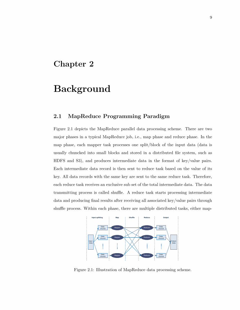
Figure 2.1 depicts the MapReduce parallel data processing scheme. There are two

major phases in a typical MapReduce job, i.e., map phase and reduce phase. In the

map phase, each mapper task processes one split/block of the input data (data is

usually chuncked into small blocks and stored in a distributed file system, such as

HDFS and S3), and produces intermediate data in the format of key/value pairs.

Each intermediate data record is then sent to reduce task based on the value of its

key. All data records with the same key are sent to the same reduce task. Therefore,

each reduce task receives an exclusive sub set of the total intermediate data. The data

transmitting process is called shuffle. A reduce task starts processing intermediate

data and producing final results after receiving all associated key/value pairs through

shuffle process. Within each phase, there are multiple distributed tasks, either map-

InputData

Datachunck

Datachunck

Datachunck

Mapper

Mapper

Mapper

Reducer

Reducer

Reducer

Datachunck

Datachunck

Datachunck

OutputData

Input splitting Map Shuffle Reduce Output

Figure 2.1: Illustration of MapReduce data processing scheme.

10

pers or reducers, running the same function independently to process their input data

sets. Therefore, data processing in each stage can be performed in parallel in a cluster

for performance improvement. If some tasks of a job fail or straggle, then only these

tasks, instead of the entire job, will be re-executed. In the MapReduce framework,

programmers only need to design appropriate map and reduce functions for their ap-

plications, without taking care of data flow, data distribution, failure recovery, and

other implementation details.

2.2 Hadoop MapReduce

The Apache Hadoop MapReduce implementation closely resembles the MapReduce

paradigm. The structure of Hadoop platform is shown in Figure 2.2. It consists of

two main components: Hadoop Distributed File System (HDFS), and MapReduce

framework. All the input and output data files are stored in HDFS, which automati-

cally chops each file into uniform sized splits, and evenly distributes all splits across

its distributed storages devices (i.e., local storages of cluster nodes). Each split of

data also has multiple redundant copies for fault tolerance and data locality. A cen-

tralized NameNode is in charge of managing the HDFS, and distributed DataNodes

are running on cluster nodes to manage the stored data.

Master Node

Slave Node Slave Node

JobTracker(scheduler)

TaskTracker(slots)

TaskTracker(slots)

NameNode(namespace)

DataNode(data chunks)

local disk

DataNode(data chunks)

local disk

Figure 2.2: Illustration of Apache Hadoop platform structure.

In a Hadoop MapReduce framework, all incoming MapReduce jobs are scheduled

and managed in a centralized master node that runs a JobTracker routine. The

map/reduce tasks of each job are executed on distributed slave nodes which run

TaskTracker routines. Resources on slave nodes are represented by the “slot” concept,

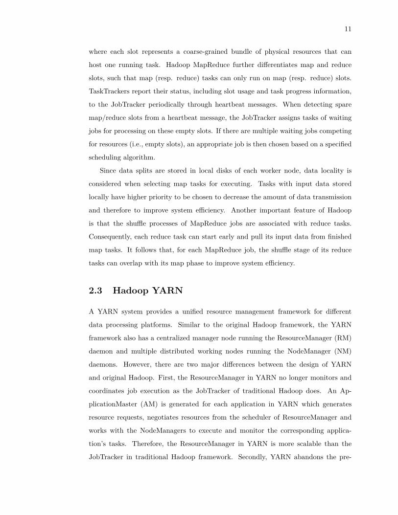
11

where each slot represents a coarse-grained bundle of physical resources that can

host one running task. Hadoop MapReduce further differentiates map and reduce

slots, such that map (resp. reduce) tasks can only run on map (resp. reduce) slots.

TaskTrackers report their status, including slot usage and task progress information,

to the JobTracker periodically through heartbeat messages. When detecting spare

map/reduce slots from a heartbeat message, the JobTracker assigns tasks of waiting

jobs for processing on these empty slots. If there are multiple waiting jobs competing

for resources (i.e., empty slots), an appropriate job is then chosen based on a specified

scheduling algorithm.

Since data splits are stored in local disks of each worker node, data locality is

considered when selecting map tasks for executing. Tasks with input data stored

locally have higher priority to be chosen to decrease the amount of data transmission

and therefore to improve system efficiency. Another important feature of Hadoop

is that the shuffle processes of MapReduce jobs are associated with reduce tasks.

Consequently, each reduce task can start early and pull its input data from finished

map tasks. It follows that, for each MapReduce job, the shuffle stage of its reduce

tasks can overlap with its map phase to improve system efficiency.

2.3 Hadoop YARN

A YARN system provides a unified resource management framework for different

data processing platforms. Similar to the original Hadoop framework, the YARN

framework also has a centralized manager node running the ResourceManager (RM)

daemon and multiple distributed working nodes running the NodeManager (NM)

daemons. However, there are two major differences between the design of YARN

and original Hadoop. First, the ResourceManager in YARN no longer monitors and

coordinates job execution as the JobTracker of traditional Hadoop does. An Ap-

plicationMaster (AM) is generated for each application in YARN which generates

resource requests, negotiates resources from the scheduler of ResourceManager and

works with the NodeManagers to execute and monitor the corresponding applica-

tion’s tasks. Therefore, the ResourceManager in YARN is more scalable than the

JobTracker in traditional Hadoop framework. Secondly, YARN abandons the pre-

12

vious coarse-grained slot configuration used by TaskTrackers in traditional Hadoop.

Instead, NodeManagers in YARN consider the fine-grained resource management for

managing various resources (e.g., CPU and memory) in the cluster. Therefore, in a

YARN system, users need to specify resource demands for each task of their jobs. A

resource request of a task is a tuple < p,~r,m, l, γ >, where p represents task priority,

~r gives a vector of task resource requirements, m shows the number of tasks in the

application which have the same resource requirements of ~r, l indicates the location

of a task’s input data split, and γ is a boolean value to indicate whether a task can be

assigned to a NodeManager that does not locally have that task’s input data split. Re-

sourceManager also receives heartbeat messages from all active NodeManagers which

report their current resource usages, and then schedules tasks to NodeManagers which

have sufficient residual resources.

Different data processing paradigms can run on top of YARN as long as appro-

priate Application Master implementations are provided. For example, a MapReduce

job’s ApplicationMaster needs to negotiate resources for its map and reduce tasks,

and coordinate the execution of map and reduce tasks, i.e., delay the start time of

reduce tasks. On the other hand, a Spark job’s ApplicationMaster needs to negotiate

resources for its executors and schedule tasks to run in the launched executors.

2.4 Scheduling Policies

Scheduling policies play an important role in large-scale data processing platforms

which are shared by multiple users and thus have the issue of resource contentions.

Classic scheduling policies that are widely adopted include FIFO, Fair, and Capacity.

• The FIFO policy sorts all waiting applications in a non-decreasing order of their

submission times. The first queuing job’s request is always scheduled for service

when there are spare resources, e.g., available slots in Hadoop MapRedce or

cpu/memory capacity in Hadoop YARN.

• The Fair policy assigns resources to applications such that all applications get,

on average, an equal share of resources over time. Job queues with different

shares and weights may be configured to support proportional resource sharing

13

for applications in different queues. A variant of Fair, named Dominant Re-

source Fairness (DRF) [21], is also widely adopted when tasks require multiple

resource types, e.g., cpu and memory. DRF assigns resources to applications

such that all applications get, on average, an equal share of their dominant

resources over time.

• The Capacity policy works similar to the Fair policy. Under Capacity, the

scheduler attempts to reserve a guaranteed resource capacity for each job queue.

Additionally, the under-utilized capacities of idle queues can be shared by other

busy queues.

When scheduling tasks for each job/application, all these scheduling policies mainly

consider data locality. Tasks with input data stored locally have higher priority to be

scheduled, such that the framework can bring computation to the data which is more

efficient than the opposite way.

14

Chapter 3

Resource Management for

Hadoop MapReduce

Hadoop MapReduce has been widely adopted as the prime framework for large-scale

data processing jobs in recent years. Although initially designed for batch job process-

ing, Hadoop MapReduce platforms usually serve much more complex workloads that

comes from multiple tenants in real world deployments. For example, Facebook [2],

one of Hadoop’s biggest champions, keeps more than 100 petabytes of Hadoop data

on-line, and allows multiple applications and users to submit their ad-hoc queries to

the shared Hive-Hadoop clusters. For those ad-hoc jobs, the average job response

time becomes a prime performance consideration in the shared Hadoop MapReduce

cluster. At the same time, the Hadoop cluster in Facebook also serves periodical batch

jobs where the total completion length of jobs is of greater importance. In this sec-

tion, we propose two different schemes for Hadoop MapReduce platform that aim to

improve the system performance under different primary performance considerations.

15

3.1 A Job Size-Based Scheduler for Hadoop

MapReduce

Scheduling policy plays an important role for improving job response times in Hadoop

when multiple users compete for available resources in cluster. However, we found

that the existing policies supported by Hadoop MapReduce platform do not perform

well in terms of job response times under heavy and diverse workloads. The default

FIFO policy, which is originally designed for better total job completion length (i.e.,

makespan) for batch jobs, performs poorly in terms of average job response time. Since

short jobs may stuck behind long jobs and have extremely long waiting time. Fair

and Capacity policies mitigate the problem of FIFO by sharing total system resources

among jobs from different queues. Such that short jobs can process immediately after

submission without waiting for long jobs if they are assigned to a different queue from

the long jobs. However, we found that Fair policy could also perform poorly in terms

of average job response times under certain workload patterns.

In this work, we introduce a scheduler, called LsPS [16, 17], which aims to im-

prove the average job response time of Hadoop MapReduce systems by leveraging the

present job size patterns to tune its scheduling schemes among users and for each

user as well. Specifically, we first develop a lightweight information collector that

tracks the important statistic information of recently finished jobs from each user. A

self-tuning scheduling policy is then designed to scheduler Hadoop jobs at two levels:

the resource shares across multiple users are tuned based on the estimated job size

of each user; and the job scheduling for each individual user is further adjusted to

accommodate to that user’s job size distribution. Experimental results in both the

simulation model and the Amazon EC2 Hadoop cluster environment confirm the ef-

fectiveness and robustness of our solution. We show that our scheduler improves the

average job response times under a variety of system workloads.

3.1.1 Motivation

In order to investigate the pros and cons of the existing Hadoop schedulers (i.e.,

FIFO and Fair), we conduct several experiments in a Hadoop MapReduce cluster at

16

Amazon EC2. In particular, we lease 11 EC2 nodes to deploy the Hadoop platform,

where one node serves as the master and the remaining ten nodes run as the slaves.

In this Hadoop cluster, each slave node contains 2 map slots and 2 reduce slots. We

run WordCount applications to compute the occurrence frequency of each word in

input files with different sizes. Randomtextwriter is used to generate random files as

the inputs of WordCount application in the experiments.

3.1.1.1 How to Share Slots

Specifically, there are two tiers of scheduling in a Hadoop system which is shared by

multiple users: (1) Tier 1 is responsible for assigning free slots to active users; and (2)

Tier 2 schedules jobs for each individual user. In this subsection, we first investigate

different Hadoop scheduling policies at Tier 1. When no minimum share of each user

is specified, Fair scheduler fairly allocates available slots among users such that all

users get an equal share of slots over time. However, we argue that Fair unfortunately

is inefficient in terms of job response times.

For example, we perform an experiment with two users such that user 1 submits

30 WordCount jobs to scan a random generated input file with size of 180 MB, while

user 2 submits 6 WordCount jobs at the same time to scan a random generated 1.6

GB input file. All the jobs will be submitted at roughly the same time. We set the

block size of HDFS to be equal to 30 MB. Thus, the map task number of each job

from user 2 is equal to 54 (1.6GB/30MB), while each job from user 1 only has 6

(180MB/30MB) map tasks. We also set the reduce task number of each job equal to

its map task number. As the average task execution times of jobs from two users are

similar, we say that the average job size (i.e., average task number times average task

execution time) of user 2 is about 9 times larger than that of user 1.

In the context of single-user job queues, it is well known that giving preferen-

tial treatment to shorter jobs can reduce the overall expected response time of the

system, such that the shortest remaining job first (SRJF) scheduling policy gener-

ates the optimal queuing time [22]. However, directly using SRJF policy has several

drawbacks. First, the large jobs could be starved in SRJF, and SRJF lacks flexibility

when certain level of fairness or priority between users is required, which is common

in practice. Moreover, precise job size prediction before execution is also required

17

for using SRJF which is not easy to achieve in real systems. In contrast, the shar-

ing based scheduling could easily solve the starve problem and provides flexibility

to integrate fairness between users by setting up minimal shares for each user. Al-

lowing all users to run their application concurrently also helps to improve the job

size prediction accuracy in Hadoop system by getting information from finished tasks.

Motivated by this observation and the analysis of discriminatory processor sharing be-

tween multiple users in [23], we evaluate the discriminatorily share policies in Hadoop

platform. It is extremely hard and complex to find out an optimal share policy under

a dynamic environment, where user workload patterns may change frequently across

time. Therefore, we opted to heuristically assign slots that are reversely proportional

to the average job sizes of users, and dynamically tune the share over time accord-

ing to the workload pattern changes. We compare Fair policy and two variants, i.e.,

share slots proportional to the average job sizes of users (Fair V1), and reversely

proportional sharing policy (Fair V2), under the two user scenario.

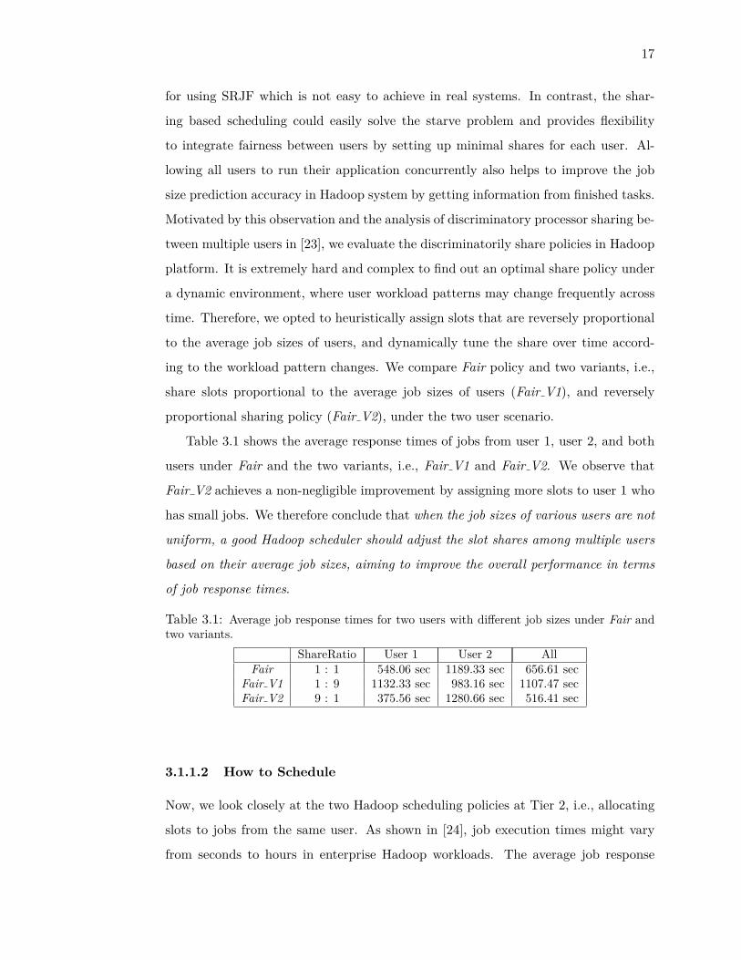
Table 3.1 shows the average response times of jobs from user 1, user 2, and both

users under Fair and the two variants, i.e., Fair V1 and Fair V2. We observe that

Fair V2 achieves a non-negligible improvement by assigning more slots to user 1 who

has small jobs. We therefore conclude that when the job sizes of various users are not

uniform, a good Hadoop scheduler should adjust the slot shares among multiple users

based on their average job sizes, aiming to improve the overall performance in terms

of job response times.

Table 3.1: Average job response times for two users with different job sizes under Fair andtwo variants.

ShareRatio User 1 User 2 AllFair 1 : 1 548.06 sec 1189.33 sec 656.61 sec

Fair V1 1 : 9 1132.33 sec 983.16 sec 1107.47 secFair V2 9 : 1 375.56 sec 1280.66 sec 516.41 sec

3.1.1.2 How to Schedule

Now, we look closely at the two Hadoop scheduling policies at Tier 2, i.e., allocating

slots to jobs from the same user. As shown in [24], job execution times might vary

from seconds to hours in enterprise Hadoop workloads. The average job response

18

times under FIFO scheduling policy thus becomes quite unacceptable because small

jobs are often stuck behind large ones and thus experiencing long waiting times. On

the other hand, Fair scheduler solves this problem by equally assigning slots to all

jobs no matter what sizes those jobs have and thus avoiding the long wait behind

large jobs. However, the average job response time of Fair scheduler depends on the

job size distribution, similar as PS policy [25]: when job sizes have high variances,

i.e., coefficient of variation1 of job sizes CV > 1, Fair achieves better performance

(i.e., shorter average job response time) than FIFO; but this performance benefit

disappears when the job sizes become close to each other, with CV ≤ 1.

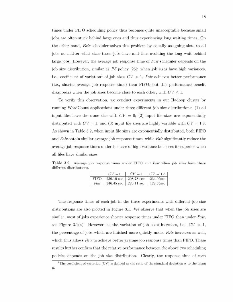
To verify this observation, we conduct experiments in our Hadoop cluster by

running WordCount applications under three different job size distributions: (1) all

input files have the same size with CV = 0; (2) input file sizes are exponentially

distributed with CV = 1; and (3) input file sizes are highly variable with CV = 1.8.

As shown in Table 3.2, when input file sizes are exponentially distributed, both FIFO

and Fair obtain similar average job response times; while Fair significantly reduce the

average job response times under the case of high variance but loses its superior when

all files have similar sizes.

Table 3.2: Average job response times under FIFO and Fair when job sizes have threedifferent distributions.

CV = 0 CV = 1 CV = 1.8FIFO 239.10 sec 208.78 sec 234.95secFair 346.45 sec 220.11 sec 128.35sec

The response times of each job in the three experiments with different job size

distributions are also plotted in Figure 3.1. We observe that when the job sizes are

similar, most of jobs experience shorter response times under FIFO than under Fair,

see Figure 3.1(a). However, as the variation of job sizes increases, i.e., CV > 1,

the percentage of jobs which are finished more quickly under Fair increases as well,

which thus allows Fair to achieve better average job response times than FIFO. These

results further confirm that the relative performance between the above two scheduling

policies depends on the job size distribution. Clearly, the response time of each1The coefficient of variation (CV) is defined as the ratio of the standard deviation σ to the mean

µ.

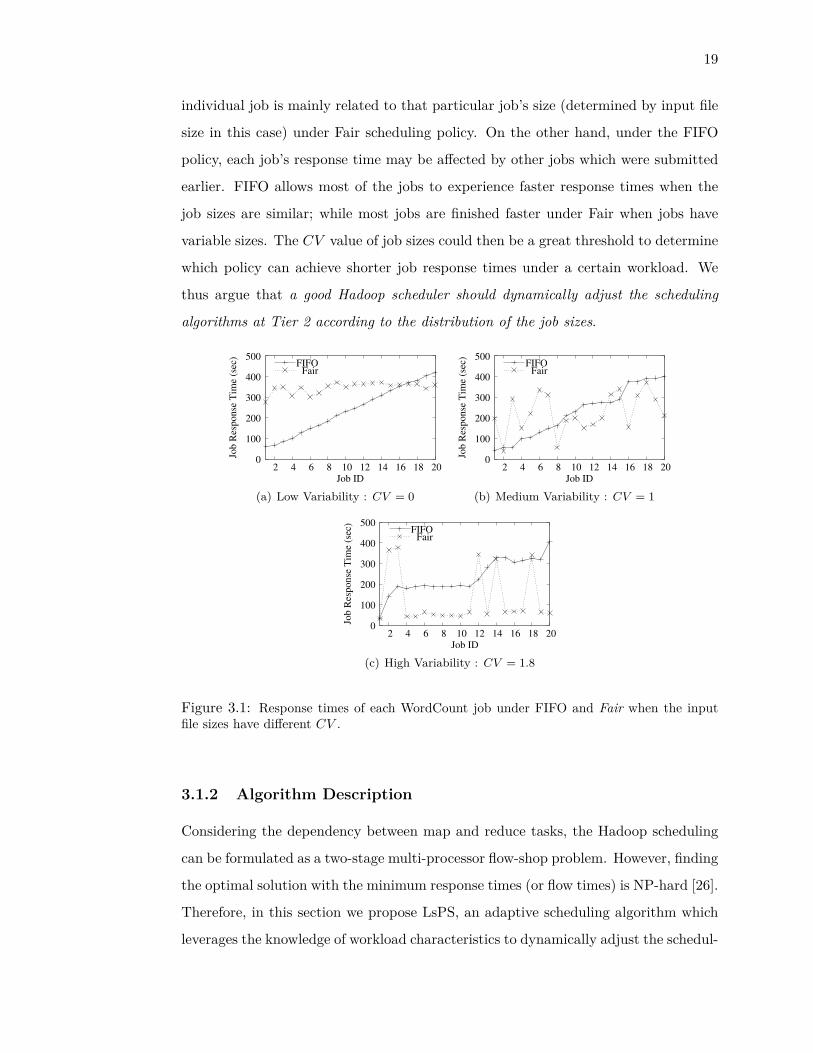
19

individual job is mainly related to that particular job’s size (determined by input file

size in this case) under Fair scheduling policy. On the other hand, under the FIFO

policy, each job’s response time may be affected by other jobs which were submitted

earlier. FIFO allows most of the jobs to experience faster response times when the

job sizes are similar; while most jobs are finished faster under Fair when jobs have

variable sizes. The CV value of job sizes could then be a great threshold to determine

which policy can achieve shorter job response times under a certain workload. We

thus argue that a good Hadoop scheduler should dynamically adjust the scheduling

algorithms at Tier 2 according to the distribution of the job sizes.

0

100

200

300

400

500

2 4 6 8 10 12 14 16 18 20

Job

Res

po

nse

Tim

e (s

ec)

Job ID

FIFOFair

(a) Low Variability : CV = 0

0

100

200

300

400

500

2 4 6 8 10 12 14 16 18 20Jo

b R

esp

on

se T

ime

(sec

)

Job ID

FIFOFair

(b) Medium Variability : CV = 1

0

100

200

300

400

500

2 4 6 8 10 12 14 16 18 20

Job

Res

po

nse

Tim

e (s

ec)

Job ID

FIFOFair

(c) High Variability : CV = 1.8

Figure 3.1: Response times of each WordCount job under FIFO and Fair when the inputfile sizes have different CV .

3.1.2 Algorithm Description

Considering the dependency between map and reduce tasks, the Hadoop scheduling

can be formulated as a two-stage multi-processor flow-shop problem. However, finding

the optimal solution with the minimum response times (or flow times) is NP-hard [26].

Therefore, in this section we propose LsPS, an adaptive scheduling algorithm which

leverages the knowledge of workload characteristics to dynamically adjust the schedul-

20

ing schemes, aiming to improve efficiency in terms of job response times in systems,

especially under heavy-tailed workloads [27].

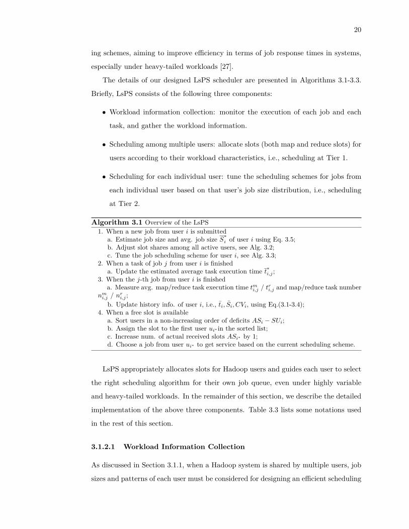
The details of our designed LsPS scheduler are presented in Algorithms 3.1-3.3.

Briefly, LsPS consists of the following three components:

• Workload information collection: monitor the execution of each job and each

task, and gather the workload information.

• Scheduling among multiple users: allocate slots (both map and reduce slots) for

users according to their workload characteristics, i.e., scheduling at Tier 1.

• Scheduling for each individual user: tune the scheduling schemes for jobs from

each individual user based on that user’s job size distribution, i.e., scheduling

at Tier 2.

Algorithm 3.1 Overview of the LsPS1. When a new job from user i is submitted

a. Estimate job size and avg. job size S∗i of user i using Eq. 3.5;b. Adjust slot shares among all active users, see Alg. 3.2;c. Tune the job scheduling scheme for user i, see Alg. 3.3;

2. When a task of job j from user i is finisheda. Update the estimated average task execution time t∗i,j ;

3. When the j-th job from user i is finisheda. Measure avg. map/reduce task execution time tmi,j / tri,j and map/reduce task number

nmi,j / nr

i,j ;b. Update history info. of user i, i.e., ti, Si, CVi, using Eq.(3.1-3.4);

4. When a free slot is availablea. Sort users in a non-increasing order of deficits ASi − SUi;b. Assign the slot to the first user ui∗ in the sorted list;c. Increase num. of actual received slots ASi∗ by 1;d. Choose a job from user ui∗ to get service based on the current scheduling scheme.

LsPS appropriately allocates slots for Hadoop users and guides each user to select

the right scheduling algorithm for their own job queue, even under highly variable

and heavy-tailed workloads. In the remainder of this section, we describe the detailed

implementation of the above three components. Table 3.3 lists some notations used

in the rest of this section.

3.1.2.1 Workload Information Collection

As discussed in Section 3.1.1, when a Hadoop system is shared by multiple users, job

sizes and patterns of each user must be considered for designing an efficient scheduling

21

Table 3.3: Notations used in the algorithm.

U / ui number of users / i-th user, i ∈ [1, U ]Ji / jobi,j set of all user i’s jobs / j-th job of user i. jobi,j ∈ Ji.tmi,j / tri,j average map/reduce task execution time of jobi,j

tmi / tri average map/reduce task execution time of jobs from ui

nmi,j / nr

i,j number of map/reduce tasks in jobi,j

si,j size of jobi,j , i.e., total exe. time of map and reduce tasksSi / S∗i average size of completed/current jobs from ui

CVi / CV ∗i coefficient of variation of completed/current job sizes of ui

SUi / SJi,j the slot share of ui / the slot share of jobi,j

ASi the slot share that ui actually received

algorithm. Therefore, a light-weight history information collector is introduced in

LsPS for collecting the important historic information of jobs and users upon each

job’s completion time. Here we collect and update the information of each job’s

map and reduce tasks separately, through the same functions. To avoid redundant

description, we use the term task to represent both types of tasks and the term size

to represent size of either map phase or reduce phase of each job as follows.

In LsPS, the important history workload information that needs to be collected

for each user ui includes its average task execution time tmi (and tri ), average size Si,

and the coefficient of variation of sizes CVi. We here adopt the Welford’s one-pass

algorithm [28] to on-line update these statistics as follows.

si,j = tmi,j · nmi,j + tri,j · nri,j , (3.1)

Si = Si + (si,j − Si)/j, (3.2)

vi = vi + (si,j − Si)2 · (j − 1)/j, (3.3)

CVi =√vi/j/Si, (3.4)

where si,j denotes the size of the j-th completed job of user ui(i.e., jobi,j), tmi,j(resp. tri,j) represents the measured average map (resp. reduce) task execution time

of jobi,j , nmi,j (resp. nri,j) means the measured map (resp. reduce) task number of

the jobi,j . We remark that a job’s size si,j is calculated here as the summation of

the execution times of all tasks from that particular job, which is independent on the

level of task concurrency, i.e., concurrently running multiple map (or reduce) tasks of

that job. Additionally, vi/j denotes the variance of ui’s job sizes. Si and vi are both

initialized as 0 and updated each time when a new job is finished and its information

22

is collected. The average map (resp. reduce) task execution time tmi (resp. tri ) can be

updated as well with Equations (3.2-3.4) by replacing si,j with tmi,j (resp. tri,j).

We use a moving window to collect and update the workload information of each

user. Let TW be a window for monitoring the past scheduling history. In each

monitoring window, the system completes exactly W jobs; we set W = 100 in all

the experiments presented in the paper. We also assume that the scheduler is able

to correctly measure the information of each completed job, such as its map/reduce

execution times as well as the number of map/reduce tasks. We remark that this

assumption should be reasonable for most Hadoop systems.

Upon each job’s completion, LsPS updates the workload statistics for job owner

using the above equations, i.e., Eq.s(3.1)-(3.4). The statistic information collected in

the present monitoring window will then be utilized by LsPS to tune the schemes for

scheduling the following W jobs arriving in the next window, see Algorithm 3.1 step

3.

3.1.2.2 Scheduling Among Multiple Users

In this subsection, we present our algorithm (i.e., Algorithm 2) for scheduling among

multiple users. Our goal is to decide the deserved amount of slots and allocate ap-

propriate number of slots for each active user to run their jobs. In a MapReduce

system, there are two types of slots, i.e., map slots and reduce slots. Therefore, we

have designed two algorithms, one for allocating map slots and the other for allocat-

ing reduce slots. However, they share the same design. For simplicity, we present a

general form of the algorithm in the rest of this subsection. We use the general terms

similar as in Section 3.1.2.1 to represent both type of tasks.

Basically, our solution is motivated by the drawbacks of Fair scheduler, which

generates long average job response times when the job sizes of multiple users vary a

lot (see Section 3.1.1.1). We found that tuning the slot share ratio among users based

on their average job sizes can help reduce the average job response times. Therefore,

we propose to adaptively adjust the slot shares among all active users such that

the share ratio is inversely proportional to the ratio of their job average sizes. For

example, in a simple case of two users, if their average job size ratio is equal to 1:2,

then the number of slots assigned to user 1 will be twice that to user 2. Consequently,

23

Algorithm 3.2 Tier 1: Allocate slots for each userInput: historic information of each active user;Output: slot share SUi of each active user;for each user ui do

Update that user’s slot share SUi using Eq.3.6;for j-th job of user i, i.e., jobi,j do

if the current job scheduling based on job submission times thenif jobi,j has the earliest submission time in pool Ji thenSJi,j = SUi;

elseSJi,j = 0;

end ifelseSJi,j = SUi/|Ji|.

end ifend for

end for

LsPS implicitly gives higher priority to users with smaller jobs, resulting in shorter

job response times.

One critical issue that needs to be addressed is how to correctly measure the

execution times of map or reduce phase of jobs that are currently running or waiting

for the service. In Hadoop systems, it is not possible to get the exact execution

times of job’s tasks before it is finished. However, the job sizes are predictable in

Hadoop system as discussed before in this section. In this work, we estimate the job

sizes as “task number” times “average task execution time”, through the following

steps: (1) the number of tasks of j-th job from user i (jobi,j), i.e., ni,j , could be

obtained immediately when the job is submitted; (2) similar to [29], we assume that

the execution times of tasks from the same job are close to each other, and thus the

average task execution time, t∗i,j , of the finished tasks of current running job jobi,j

could be used to represent the overall average task execution time ti,j of that job;

and (3) for those jobs that are still waiting for execution or jobs that are currently

running but have no finished tasks, we consider the historic information and use the

average task execution times of recently finished jobs from their user ui, e.g., ti, to

approximate their average task execution time ti,j .

Therefore, user ui’s average map phase size of jobs is calculated as follows,

S∗i = 1|Ji|·|Ji|∑j=1

nmi,j · tmi,j , (3.5)

where Ji represents the set of jobs from user ui that are currently running or waiting

24

for service. And the average reduce phase size of ui could be calculated in the same

way. We remark that due to dynamic changes in the workloads, instead of calculating

the average map phase size of all the jobs that are submitted by a user, we only

take the jobs that are currently running or waiting in the queue into consideration

of job size calculation. Particularly, our scheduler recalculates the average job sizes

and updates the slots assignment among users upon the submission time of new jobs.

Therefore, our scheduler can adapt to the changes in the job sizes of each user by

dynamically tuning the slot assignment.

As shown in Algorithm 3.2 step 1, once a new job arrives, LsPS updates the

average size of that job’s owner and then adaptively adjusts the deserved map slot

shares (SUi) among all active users using Eq.(3.6).

SUi = SU∗i · (α · U ·1S∗i∑Ui=1

1S∗i

+ 1− α), (3.6)

∀i, SUi > 0, (3.7)U∑i=1

SUi =U∑i=1

SU∗i , (3.8)

where SU∗i represents the deserved slot shares for user ui under the Fair scheme, i.e.,

equally dispatching the slots among all users, U indicates the number of users that

are currently active in the system, and α is a tuning parameter within the range from

0 to 1. Parameter α in Eq.(3.6) can be used to control how aggressively LsPS biases

towards the users with smaller jobs: when α is close to 0, our scheduler increases the

degree of fairness among all users, performing similar as Fair; and when α is increased

to 1, LsPS gives the strong bias towards the users with small jobs in order to improve

the efficiency in terms of job response times. In the remainder of the paper, we set α

as 1 if there is no explicit specification. We remark that when all users have the same

average job sizes, one can get SUi equal to SU∗i , i.e., fairly allocating slots among

users. We also note that when using Eq.(3.6) to calculate the SUi for each user, it is

guaranteed that no active users gets starved for map/reduce slots, see Eq.(3.7), and

all available slots in the system are fully distributed to active users, see Eq.(3.8).

The resulting deserved slot shares (i.e., SUi) are not necessarily equal to the actual

assignments among users (i.e., ASi). They will be used to determine which user can

receive the slot that just became available for redistribution, see Algorithm 3.2 step

25

2. LsPS sorts all active users in a non-increasing order of their deficits, i.e., the gap

between the expected assigned slots (SUi) and the actual received slots (ASi), and

then dispatchs that particular slot to the user with the largest deficit. Additionally,

it might happen in the Hadoop system that some users have high deficits but their

actual demands on map/reduce slots are less than the expected shares. In such a

case, LsPS re-dispatches the extra slots to those users who have lower deficits but

need more slots for serving their jobs.

3.1.2.3 Scheduling for A User

The second design principle used in LsPS is to dynamically tune the scheduling scheme

for jobs within an individual user by leveraging the knowledge of job size distribution.

As observed in Section 3.1.1.2, the scheme of equally distributing shared resources

outperforms by avoiding small jobs to waiting behind large ones. However, when

the jobs have similar sizes, scheduling jobs based on their submission times becomes

superior to the former one.

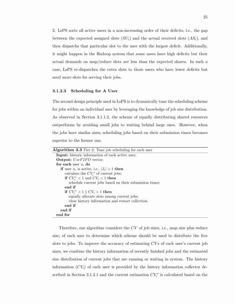
Algorithm 3.3 Tier 2: Tune job scheduling for each userInput: historic information of each active user;Output: UseFIFO vector;for each user ui do

if user ui is active, i.e., |Ji| > 1 thencalculate the CV ∗i of current jobs;if CV ∗i < 1 and CVi < 1 then

schedule current jobs based on their submission times;end ifif CV ∗i > 1 ‖ CVi > 1 then

equally allocate slots among current jobs;clear history information and restart collection.

end ifend if

end for

Therefore, our algorithm considers the CV of job sizes, i.e., map size plus reduce

size, of each user to determine which scheme should be used to distribute the free

slots to jobs. To improve the accuracy of estimating CV s of each user’s current job

sizes, we combine the history information of recently finished jobs and the estimated

size distribution of current jobs that are running or waiting in system. The history

information (CVi) of each user is provided by the history information collector de-

scribed in Section 3.1.2.1 and the current estimation CV ∗i is calculated based on the

26

estimated job sizes described in Section 3.1.2.2. When the two values of a user are

both smaller than 1, the LsPS scheme schedules the current jobs in that user’s sub

queue in the order of their submission times, otherwise the user level scheduler will

fairly assign slots among jobs. When the two values are conflicting, i.e., CVi > 1 and

CV ∗i < 1 or vise versa, which means the user’s workload pattern may change, the fair

scheme will be adopted at this time, and the history information will be cleared and

a new collection window will start at this time, see the pseudo-code in Algorithm 3.3.

3.1.3 Model Description

In this section, we introduce a model that is developed to emulate a classic Hadoop

system. The purpose of this model is twofold: 1) to capture the actual execution of

Hadoop jobs with multiple map and reduce tasks; and 2) to compare various Hadoop

scheduling schemes and give the first proof of our new approach. Later, we will

evaluate the performance of these schemes in a real Hadoop system.

... ...

Sm Map Slots

Map Queue (Qm)

Sr Reduce Slots

{m_n,m_t,r_n,r_t}

Job Generator

Update Percentage of Finished Map Tasks for Each Job

Reduce Queue (Qr)

Map Task

Dispatcher

Reduce TaskDispatcher

Figure 3.2: Modeling a Hadoop MapReduce cluster.

The model, as shown in Fig. 3.2, consists of two queues for map tasks (Qm) and

reduce tasks (Qr), respectively. Once a job is submitted, its tasks will be inserted

into Qm (resp. Qr) through the map (resp. reduce) task dispatcher. Furthermore,

the model includes s servers to represent s available slots in the system, such that

sm servers are used to serve map tasks while the remaining servers, i.e., sr = s− sm,

connect to the reduce queue for executing reduce tasks. Note that the values of

{sm, sr} are based on the actual Hadoop configuration.

27

An important feature of MapReduce jobs need to be considered in the model is

the dependency between map and reduce tasks. Typically, in a Hadoop cluster, there

is a parameter which decides when a job can start its reduce tasks. By default, this

parameter is set as 5%, which indicates that the first reduce task can be launched

when 5% of the map tasks are committed. Under this setting, a job’s first wave of

reduce tasks will overlap with its map phase and could prefetch the output of map

tasks in the overlapping period. However, previous work [30] found that this setting

would lead to performance degradation under the Fair scheduling policy and proposed

to launch reduce tasks gradually according to the progress of map phase. We further

found that delaying the launch time of reduce tasks, i.e., setting the parameter to

a large value such as 100%, can improve the performance of the Fair and the other

slots sharing based schedulers. Therefore, in our experiments, we set the parameter

to 100%, i.e., running reduce tasks when all map tasks are completed, in all the

three policies (i.e., FIFO, Fair and our LsPS). However, we remark that this is not

a necessary assumption. Our scheduler works in the same way under the other two

cases, i.e., launching the first reduce task when 5% of the map tasks are committed

or launching the reduce tasks gradually according to the progress of map phase.

3.1.4 Evaluation

In this section, we turn to present the performance evaluation of the proposed LsPS

scheduler, which aims to improve the efficiency of a Hadoop system, especially with

highly variable and/or bursty workloads from different users.

3.1.4.1 Simulation Evaluation

We first evaluate LsPS with our simulation model which is developed to emulate

a classic Hadoop system. On top of this model, we use trace-driven simulations to

evaluate the performance improvement of LsPS in terms of average job response times.

Later, we will verify the performance of LsPS by implementing the proposed policy

as a plug-in scheduler in an EC2 Hadoop cluster.

In our simulations, we have U users {u1, ..., ui, ..., uU} to share the Hadoop cluster

by submitting Ji jobs to the system. The specification of users include their job inter-

arrival times and job sizes, which are created based on the specified distributions and

28

23%37%

13%

37%62%60%

(b) User 1

36%−0.4%

−1%

(c) User 2

100

1000

10000

100000

u:u u:h u:b Aver

age

Res

ponse

Tim

e (S

ec) (a) Overall

100

1000

10000

100000

u:u u:h u:b Aver

age

Res

ponse

Tim

e (S

ec)

100

1000

10000

100000

u:u u:h u:b Aver

age

Res

ponse

Tim

e (S

ec)

LsPSFairFIFO

Figure 3.3: Average job response times of (a) two users, (b) user 1, and (c) user 2 underthree different scheduling policies, i.e., FIFO, Fair and LsPS. Here, user 1 has uniform job sizedistribution while user 2 have similar job sizes (see the bars denoted as u:u); high variability injob sizes (see the bars denoted as u:h); and high variability and strong temporal dependencein job sizes (see the bars denoted as u:b). The relative improvement with respect to Fair isalso plotted on each bar of LsPS.

0.001

0.01

0.1

1

10 100 1000 10000 100000

CC

DF

Response Time (sec)

FIFOFair

LsPS 0.001

0.01

0.1

1

10 100 1000 10000 100000 1e+06

CC

DF

Response Time (sec)

FIFOFair

LsPS 0.001

0.01

0.1

1

10 100 1000 10000 100000 1e+06

CC

DF

Response Time (sec)

FIFOFair

LsPS

(a) Job Size Pattern u:u (b) Job Size Pattern u:h (c) Job Size Pattern u:b

Figure 3.4: CCDFs of response times of all jobs under three different scheduling policies,where user 1 has uniform job size distribution while user 2 have (a) similar job sizes; (b) highvariability in job sizes; and (c) high variability and strong temporal dependence in job sizes.

methods. Recall that each Hadoop job size is determined by the number of map

(resp. reduce) tasks from that job as well as the execution time of each map (resp.

reduce) task. In our model, we consider to change the distributions of map/reduce

task numbers for investigating various job size patterns, while fixing the uniform

distribution to draw the execution times of map/reduce tasks.

In general, we consider the following four different distributions to generate job

inter-arrival times and job map/reduce task numbers.

• Uniform distribution (u), which indicates similar job sizes.

• Exponential distribution (e), which implies medium diversity of job sizes or

inter-arrival times.

• Hyper-exponential distribution (h), which means high variance of traces.

• Bursty pattern (b), which indicates high variance and high auto-correlation of

traces.

29

We first consider two simple cases where the Hadoop cluster is shared by two

users. We evaluate the impacts of different job size patterns in case 1 and different

job arrival patterns in case 2. We then validate the robustness of LsPS with a complex

case where the cluster is shared by multiple users with different job size and job arrival

patterns.

Simple Case 1-Two Users with Diverse Job Size Patterns Consider a

simple case of two users, i.e., u1 and u2, that concurrently submit Hadoop jobs to the

system. We first focus on evaluating different Hadoop schedulers under various job

size patterns, i.e., we conduct experiments with different job size distributions for u2,

but always keeping the uniform distribution to generate job sizes for u1. Specifically,

we consider u2 with (1) similar job sizes; (2) high variability in job sizes; and (3)

high variability and strong temporal dependence in job sizes. We also set the job

size ratio between u1 and u2 as 1:1, i.e., two users having the same average job sizes.

Furthermore, both users have the exponentially distributed job interarrival times with

the same mean of 300 seconds.

Figure 3.3 shows the mean job response times of both users under the different

policies and the relative improvement with respect to Fair. The mean job response

times of each user are presented in the figure as well. Job response time is measured

from the moment when that particular job is submitted to the moment that all the

associated map and reduce tasks are finished. We first observe that high variability

in job sizes dramatically degrades the performance under FIFO as a large number of

small jobs are stuck behind the extremely large ones, see plot (a) in Figure 3.3. In

contrast, both Fair and LsPS effectively mitigate such negative performance effects

by equally distributing available slots between two users and within a single user. Our

policy further improves the overall performance by shifting the scheduler to FIFO for

the jobs from u1 and thus significantly reducing its mean job response time by 60%

and 62% with respect to Fair when the job sizes of user 2 are highly variable (i.e.,

“u:h”) and temporally dependent (i.e., “u:b”), respectively, see plot (b) in Figure 3.3.

On the other hand, Fair loses its superiority when both users have similar job sizes,

while our new scheduler bases on the features of both users’ job sizes to tune the

scheduling at two tiers and thus achieves the performance close to the best one.

To further investigate the tail of job response times, we plot in Figure 3.4 the

30

complementary cumulative distribution functions (CCDFs) of job response times, i.e.,

the probability that the response times experienced by individual jobs are greater than

the value on the horizontal axis, for both users under the three scheduling policies.

Consistently, almost all jobs from the two users experience shorter response times

under Fair and LsPS than under FIFO when job sizes of u2 are highly variable. In

addition, compared to Fair, LsPS reduces the response times for more that 60% of

jobs, having shorter tails in job response times.

(I) Job Size Ratio 1:10

31% 27%19%

26% 21% 32%

36% 7%

−5%

(II)

31%19%

18%

36% 35%58%

26%

7%

3%

Job Size Ratio 10:1

100

1000

10000

100000

u:u u:h u:b Av

erag

e R

esp

on

se T

ime

(Sec

) (a) Overall

100

1000

10000

100000

u:u u:h u:b Av

erag

e R

esp

on

se T

ime

(Sec

) (b) User 1

100

1000

10000

100000

u:u u:h u:b Av

erag

e R

esp

on

se T

ime

(Sec

) (c) User 2

100

1000

10000

u:u u:h u:bAv

erag

e R

esp

on

se T

ime

(Sec

) (c) User 2

100

1000

10000

u:u u:h u:bAv

erag

e R

esp

on

se T

ime

(Sec

) (a) Overall

100

1000

10000

u:u u:h u:bAv

erag

e R

esp

on

se T

ime

(Sec

) (b) User 1

FairFIFO LsPS

Figure 3.5: Average job response times of (a) two users, (b) user 1, and (c) user 2 underthree different scheduling policies. The relative job size ratio between two users is (I) 1:10,and (II) 10:1.

(II) Job Size Ratio 10:1

(I) Job Size Ratio 1:10

0.001

0.01

0.1

1

10 100 1000 10000 100000 1e+06

CC

DF

Response Time (sec)

(c) Job Size Pattern u:b

FIFOFair

LsPS 0.001

0.01

0.1

1

10 100 1000 10000 100000 1e+06

CC

DF

Response Time (sec)

(b) Job Size Pattern u:h

FIFOFair

LsPS 0.001

0.01

0.1

1

10 100 1000 10000 100000

CC

DF

Response Time (sec)

(a) Job Size Pattern u:u

FIFOFair

LsPS

0.001

0.01

0.1

1

10 100 1000 10000 100000

CC

DF

Response Time (sec)

(b) Job Size Pattern u:h

FIFOFair

LsPS 0.001

0.01

0.1

1

10 100 1000 10000 100000

CC

DF

Response Time (sec)

(c) Job Size Pattern u:b

FIFOFair

LsPS 0.001

0.01

0.1

1

10 100 1000 10000 100000

CC

DF

Response Time (sec)

(a) Job Size Pattern u:u

FIFOFair

LsPS

Figure 3.6: CCDFs of response times of all jobs under three different scheduling policies.The relative job size ratio between two users is (I) 1:10, and (II) 10:1.

31

In order to analyze the impacts of relative job sizes on LsPS performance, we

conduct another two sets of experiments with various job size ratios between two

users, i.e., we keep the same parameters as the previous experiments but tune the

job sizes of u2 such that we have the average job size of u1 is 10 times less (resp.

more) than that of u2, see the results shown in Figure 3.5(I) (resp. Figure 3.5(II)).

In addition, we tune the job arrival rates of u2 to keep the same loads in the system.

Recall that our LsPS scheduler always gives higher priority, i.e., assigning more slots,

to the user with smaller average job size, see Section 3.1.2.2. As a result, LsPS

achieves non-negligible improvements of overall job response times no matter which

user has smaller job sizes, see plots (a) in Figure 3.5(I) and (II). Further confirmation

of this benefit comes from the plots in Figure 3.6(I) and (II), which show that most

jobs experience the shortest response times when the scheduling is LsPS. Indeed, the

part of the workload whose job sizes are large receives increased response times, but

the number of penalized jobs is less than 5% of the total.

We also observe that under the cases of two different job size ratios, LsPS always

achieves significant improvement in job response times for the user which submits

small jobs in average by assigning more slots to that user, see plot (b) in Figure 3.5(I)

and plot (c) in Figure 3.5(II). Meanwhile, although LsPS discriminately treats another

user (i.e., having larger jobs) with less resource, this policy does not always sacrifice

that user’s performance. For example, as shown in plot (c) of Figure 3.5(I), when

job sizes of u2 are highly variable and/or strongly dependent, shorter response times

are achieved under LsPS or Fair than under FIFO because small jobs now have the

reserved slots without waiting behind the large ones. Another example can be found

in plot (b) of Figure 3.5(II), where we observe that LsPS is superior to Fair on the

performance of user 1 by switching the tier 2 scheduling algorithm to FIFO.

Simple Case 2-Two Users with Diverse Job Arrival Patterns We now

turn to consider the changes in job arrival patterns. We conduct experiments with

varying arrival processes of the second user, i.e., u2, but always fixing the uniform job

size distributions for both users as well as the relative job size ratio between them as

1:10. Therefore, the job interarrival times of u2 are drawn from three different arrival

patterns, i.e., exponential, hyper-exponential and bursty, while user 1’s job interarrival

times are exponentially distributed in all the experiments. We then depict the average

32

58%

60%

31%26%

65%

61%36%

26%

46%

100

1000

10000

e:e e:h e:bAver

age

Res

ponse

Tim

e (S

ec) (b) User 1

100

1000

10000

e:e e:h e:bAver

age

Res

ponse

Tim

e (S

ec) (c) User 2

100

1000

10000

e:e e:h e:bAver

age

Res

ponse

Tim

e (S

ec) (a) Overall

FIFO Fair LsPS

Figure 3.7: Average job response times of (a) two users, (b) user 1, and (c) user 2 under threedifferent scheduling policies, i.e., FIFO, Fair and LsPS. Here, job interarrival times of usersare exponentially distributed while user 2’s arrival process is exponential (see the bars denotedas e:e); hyper-exponential (see the bars denoted as e:h); and bursty (see the bars denoted ase:b). The relative job size ratio between two users is 1:10. The relative improvement withrespect to Fair is also plotted on each bar of LsPS.

0.001

0.01

0.1

1

10 100 1000 10000 100000

CC

DF

Response Time (sec)

(a) Arrival Pattern e:e

FIFOFair

LsPS 0.001

0.01

0.1

1

10 100 1000 10000 100000

CC

DF

Response Time (sec)

(b) Arrival Pattern e:h

FIFOFair

LsPS 0.001

0.01

0.1

1

10 100 1000 10000 100000 1e+06

CC

DF

Response Time (sec)

(c) Arrival Pattern e:b

FIFOFair

LsPS

Figure 3.8: CCDFs of job response times under three different scheduling policies, i.e., FIFO,Fair and LsPS, where job interarrival times of users are exponentially distributed while user2’s arrival process is (a) exponential; (b) hyper-exponential; and (c) bursty. The relative jobsize ratio between two users is 1:10.

job response times of two users in Figure 3.7 and the CCDFs of job response times in

Figure 3.8.

Consistent to the previous experiments, our LsPS scheduler outperforms in terms

of the overall job response times, see plot (a) in Figure 3.7. We observe that this

benefit indeed comes from the response time improvement of u1, i.e., LsPS assigns

u1 with more slot shares due to its smaller average job size and further schedules its

jobs based on the FIFO discipline because its job sizes have low variability. However,

comparing to FIFO, this outcome unfortunately penalizes user 2, especially when

this user’s arrival process is hyper-exponential or bursty, see plot (c) in Figure 3.7.

Meanwhile, due to the uniform job size distribution, LsPS schedules the jobs from

u2 in the order of their submission times, which indeed compensates for the less

resources and thus reduces the average response time when compared to Fair. The

CCDFs shown in Figure 3.8 further confirm that a large portion of jobs experiences

the shortest response times under LsPS than under the other two policies.

Complex Case-Multiple Users with Diverse Job Arrival/Size Patterns

33

To further verify the robustness of LsPS, we conduct experiments under a more com-

plex case of 6 users which have the mixed workloads of varying job arrival and job

size patterns. Table 3.4 presents the detailed experimental settings. Here, users with

larger IDs have relatively larger job sizes in average. We also adjust the average ar-

rival rate of each user such that all the users submit the same load to the system.

Table 3.5 and Figure 3.9 present the average job response times as well as the distri-

butions of job response times of all users under the three different scheduling policies,

i.e., FIFO, Fair and LsPS. The average job response times of each user are also shown

in the table. Furthermore, in order to analyze the impact of parameter α in Eq. 3.6,

Table 3.4 shows the simulation results under LsPS with α equal to 0.3, 0.6 and 1.0.

Table 3.4: Experimental settings for each user.

User Job Size Pattern Job Arrival Pattern Average Job Size Ratio1 Bursty Hyper-exponential 12 Exponential Exponential 53 Uniform Exponential 104 Hyper-exponential Exponential 205 Uniform Bursty 506 Hyper-exponential Hyper-exponential 100

We first observe that LsPS with different α significantly improves the overall job

response times compared to FIFO and Fair. Meanwhile, the average response times

of the first four users are improved as well under LsPS because those users have

relatively smaller job sizes and thus receive more map/reduce slots for executing their

jobs. On the other hand, although the last two users u5 and u6 are assigned with the

least number of slots, their average job response times have not been dramatically

increased. In contrast, their jobs even experience faster response times compared to

Fair for u5 and to Fair and FIFO for u6. The main reason is because LsPS switches the

scheduling for each user between FIFO and Fair based on their job size distributions

and thus improves that particular user’s response times. Additionally, LsPS completes

the jobs from the first four users within a short time period such that the occupied

slots will be released soon and then reassigned to the last two users, which further

decreases the job response times of these two users.

Recall that parameter α in Eq. 3.6 is a tuning parameter to control how ag-

gressively LsPS discriminates large jobs from small ones. The larger the α is, the

34

stronger bias is given towards the users with small jobs. Table 3.5 shows that LsPS

with α = 1.0 introduces the strongest bias on user slot shares and achieves the best

response time improvement. Therefore, we set α = 1.0 in the remainder of this paper.

Table 3.5: Average response times (in seconds) of all users and each user under differentscheduling policies.

User FIFO Fair LsPS LsPS LsPSα = 0.3 α = 0.6 α = 1.0

1 7357.60 211.43 163.00 150.05 142.512 11520.03 283.43 234.64 222.00 220.203 10822.45 475.00 276.18 258.88 254.414 10626.55 1182.14 742.41 734.50 647.845 12017.48 40677.55 22637.01 17557.73 13317.926 11346.46 3318.84 3194.37 4760.66 5587.35

All 8488.00 939.24 583.05 505.94 441.66

0.001

0.01

0.1

1

10 100 1000 10000 100000

CC

DF

Response Time (sec)

FIFOFair

LsPS

Figure 3.9: CCDFs of job response times under different scheduling policies under the com-plex case of 6 users having the mixed workloads.

3.1.4.2 Case Studies in Amazon EC2

To further verify the effectiveness and robustness of our new scheduler, we implement

and evaluate the LsPS algorithms in Amazon EC2, a cloud platform that provides

pools of computing resources to developers for flexibly configuring and scaling their

computational capacity on demand.

Experimental Setting In particular, we lease a m1.large instance as master

node, which provides 2 virtual cores with 2 EC2 Compute Units each, 7.5 GB memory,

and 850 GB storage to perform heartbeat and jobtracker routines for job scheduling.

We also use the same 11 m1.large instances to launch slave nodes, each of which is

configured with two map slots and two reduce slots. Such a configuration ensures

35

that the system bottleneck is not our scheduler on master node, while the overall

job response times depend on the scheduling algorithms as well as the processing

capability of each slave node.

As the Hadoop project provides APIs to support pluggable schedulers, we im-

plement our proposed LsPS scheduling policy in Amazon Hadoop by extending the

TaskScheduler interface. In particular, we add a module in our scheduler to peri-

odically predict the job sizes of users based on the execution times of finished tasks

(which are recorded for logging purpose in original Hadoop implementation). We also

integrate another module to calculate the slot share between users upon the submis-

sion of new jobs and assign tasks of different users according to the deficiency between

their running tasks and deserved slot assignments.

The benchmarks we consider for performance evaluation includes the following

four classic MapReduce applications.

• WordCount - taking text files as job inputs and computing the occurrence fre-

quency of each word in input files. The map tasks take one line each time and

emit key/value pairs of each word in the line and count 1, and the reduce tasks

sum up the counts for each word and emit the key/value pairs of each individual

word in files and its total occurrence.

• PiEstimator - estimating the value of π using quasi-Monte Carlo method, where

map tasks generate random points in a unit square and then count the number

of points that locate inside and outside of the inscribed circle of the square,

while reduce tasks accumulate points inside/outside results from the map tasks.

• Grep - extracting and counting the strings in input files that match the given

regular expression. Each map task takes lines of input files, matches the user

provided regular expression and emits key/value pairs of matching string and

count 1. The reduce tasks then sum the frequencies of each matching string.

• Sort - taking sequential files as inputs and fragmenting and sorting the input

data. The map and reduce functions are Hadoop predefined IdentifyMapper and

IdentifyReducer which pass inputs directly to the output through the MapRe-

duce framework.

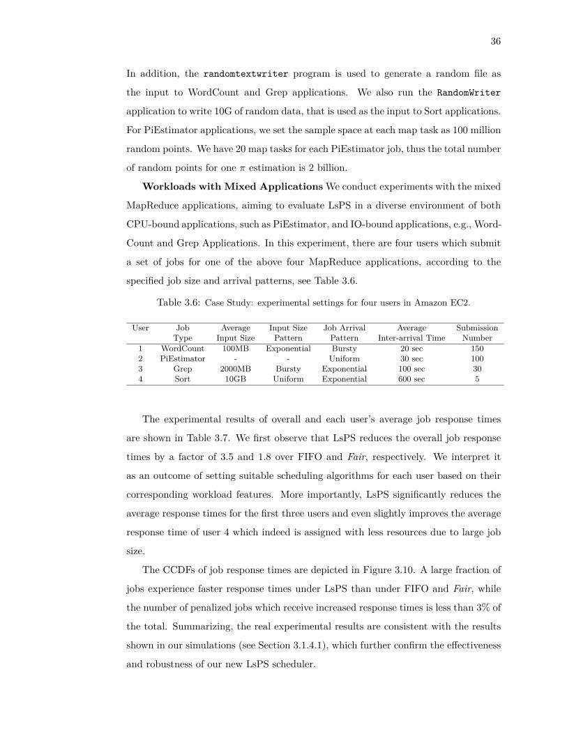
36

In addition, the randomtextwriter program is used to generate a random file as

the input to WordCount and Grep applications. We also run the RandomWriter

application to write 10G of random data, that is used as the input to Sort applications.

For PiEstimator applications, we set the sample space at each map task as 100 million

random points. We have 20 map tasks for each PiEstimator job, thus the total number

of random points for one π estimation is 2 billion.

Workloads with Mixed Applications We conduct experiments with the mixed

MapReduce applications, aiming to evaluate LsPS in a diverse environment of both

CPU-bound applications, such as PiEstimator, and IO-bound applications, e.g., Word-

Count and Grep Applications. In this experiment, there are four users which submit

a set of jobs for one of the above four MapReduce applications, according to the

specified job size and arrival patterns, see Table 3.6.

Table 3.6: Case Study: experimental settings for four users in Amazon EC2.

User Job Average Input Size Job Arrival Average SubmissionType Input Size Pattern Pattern Inter-arrival Time Number

1 WordCount 100MB Exponential Bursty 20 sec 1502 PiEstimator - - Uniform 30 sec 1003 Grep 2000MB Bursty Exponential 100 sec 304 Sort 10GB Uniform Exponential 600 sec 5

The experimental results of overall and each user’s average job response times

are shown in Table 3.7. We first observe that LsPS reduces the overall job response

times by a factor of 3.5 and 1.8 over FIFO and Fair, respectively. We interpret it

as an outcome of setting suitable scheduling algorithms for each user based on their

corresponding workload features. More importantly, LsPS significantly reduces the

average response times for the first three users and even slightly improves the average

response time of user 4 which indeed is assigned with less resources due to large job

size.

The CCDFs of job response times are depicted in Figure 3.10. A large fraction of

jobs experience faster response times under LsPS than under FIFO and Fair, while

the number of penalized jobs which receive increased response times is less than 3% of

the total. Summarizing, the real experimental results are consistent with the results

shown in our simulations (see Section 3.1.4.1), which further confirm the effectiveness

and robustness of our new LsPS scheduler.

37

Table 3.7: Average response times (in seconds) of all users and each user in the AmazonHadoop cluster.

User FIFO Fair LsPS1 251.36 121.18 67.502 280.06 149.95 74.793 235.33 118.36 75.184 330.20 248.00 209.00

All 259.61 132.90 74.16

0.001

0.01

0.1

1

10 100 1000

CC

DF

Response Time (sec)

FIFOFair

LsPS

Figure 3.10: CCDFs of job response times when four different MapReduce applications arerunning in Amazon EC2.

Non-Stationary Workloads In the previous sections, we have confirmed that

LsPS performs effectively under a stationary workload, where all users have the stable

job size/arrival patterns within the whole experiments. Now, we turn to evaluate LsPS

under non-stationary workloads, further verifying its effectiveness when the workloads

of some users change over time.

In particular, we conduct experiments with two users which submit a set of Word-

Count jobs to our Hadoop cluster consisting of 18 map and 18 reduce slots on m1.large

instances (i.e., slave nodes) in Amazon EC2. We further generate a non-stationary

workload by changing the job size/arrival patterns of user 1 while keeping fixed user

2’s input file sizes and job interarrival times both exponentially distributed with mean

of 500MB and 25 seconds, respectively. Table 3.8 illustrates the three changes in user

1’s workloads.

Table 3.8: Experimental settings for user 1’s non-stationary workload.

Periods Average Input Size Input Size Pattern Inter-arrival Time Submission #1 100MB Uniform 5 sec 502 100MB HyperExponential 5 sec 503 2500MB Uniform 125 sec 10

38

Table 3.9 shows the mean response times of two users as well as of each user

under the Fair and LsPS policies. The average job response times measured during

each period are also shown in the table. We observe that LsPS successfully captures

the changes in user 1’s workloads and dynamically tunes the two-level scheduling

(i.e., between two users and within each user) based on the measured job size/arrival

patterns. As a result, LsPS always achieves noticeable response time improvement by

26%, 24%, and 40% during the three periods and by 34% in overall with respect to

Fair.

Table 3.9: Average job response times (in seconds) of Fair and LsPS under non-stationaryworkloads

User Period 1 Period 2 Period 3 AllFair LsPS Fair LsPS Fair LsPS Fair LsPS

1 108.96 50.30 100.72 60.78 803.00 771.10 168.30 120.592 277.90 354.50 326.70 329.60 357.52 158.40 341.74 210.87

All 136.32 101.00 138.38 105.58 431.33 260.51 235.75 155.70

To better understand LsPS’s processing on non-stationary workloads, Figure 3.11

illustrates how LsPS dynamically adjusts its two-level scheduling algorithms in an

on-line fashion. Specifically, the transient distributions of 18 map slots between two

users are depicted in Figure 3.11(a), where red areas indicate the slots assigned to

user 1 while greed areas represent those assigned to user 2. We also plot the changes

of the scheduling within user 1 as a function of time in Figure 3.11(b).

As we observed, during the first period, LsPS assigns more shares to user 1 than to

user 2 because LsPS detects that user 1 has smaller average job size, see Figure 3.11(a).

Meanwhile, the jobs from user 1 are scheduled according to the FIFO discipline, see

Figure 3.11(b), which further reduces the response times of user 1 and thus results

in better overall response times during this period. Once LsPS captures the changes

in user 1’s job size distribution, i.e., from uniform to hyperexponential, LsPS quickly

switches the scheduling within user 1 from FIFO to Fair and thus consistently achieves

shorter response times in the second period, see Figure 3.11(b). Later, when user 1

starts to submit large jobs with the uniform distribution, LsPS turns to dispatch more

resources to user 2, decreasing its job response times during the last period. On the

other hand, user 1 still experiences shorter job response times than under Fair even

though this user now receives less resources. We interpret this by observing the FIFO

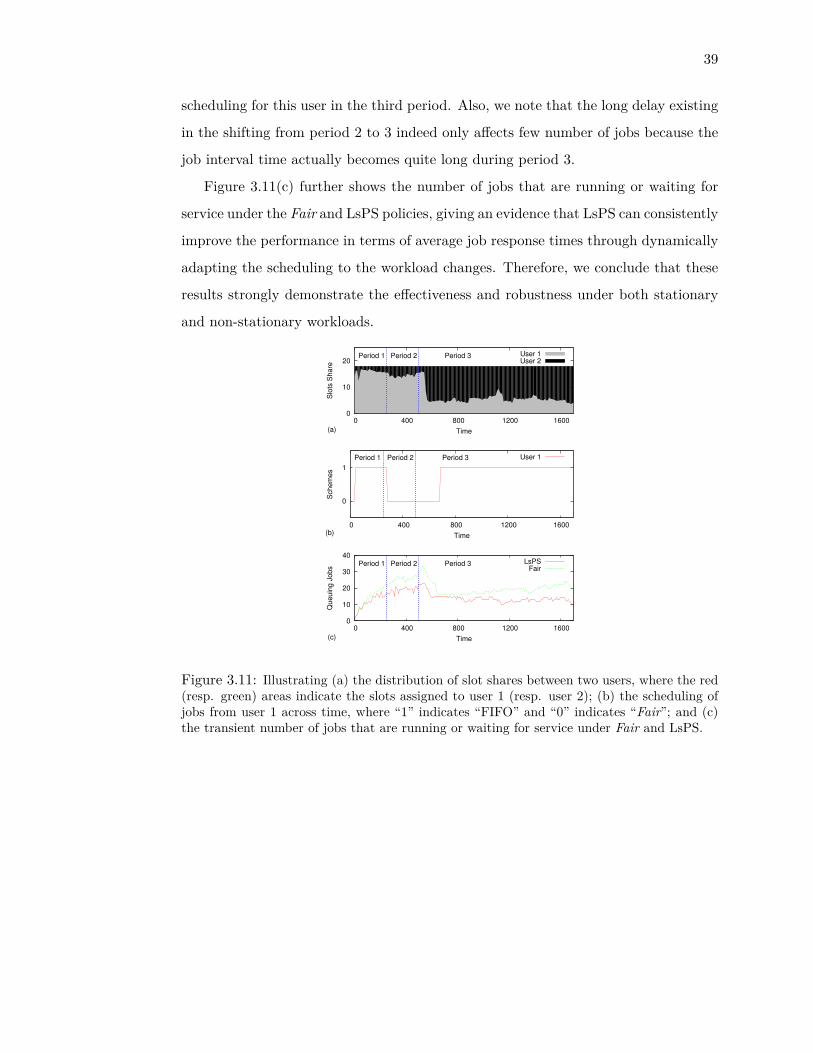
39

scheduling for this user in the third period. Also, we note that the long delay existing

in the shifting from period 2 to 3 indeed only affects few number of jobs because the

job interval time actually becomes quite long during period 3.

Figure 3.11(c) further shows the number of jobs that are running or waiting for

service under the Fair and LsPS policies, giving an evidence that LsPS can consistently

improve the performance in terms of average job response times through dynamically

adapting the scheduling to the workload changes. Therefore, we conclude that these

results strongly demonstrate the effectiveness and robustness under both stationary

and non-stationary workloads.

0

10

20

0 400 800 1200 1600

Slo

ts S

ha

re

Time(a)

Period 1 Period 2 Period 3 User 1User 2

0

1

0 400 800 1200 1600

Sch

em

es

Time(b)

Period 1 Period 2 Period 3 User 1

0

10

20

30

40

0 400 800 1200 1600

Qu

eu

ing

Jo

bs

Time(c)

Period 1 Period 2 Period 3 LsPSFair

Figure 3.11: Illustrating (a) the distribution of slot shares between two users, where the red(resp. green) areas indicate the slots assigned to user 1 (resp. user 2); (b) the scheduling ofjobs from user 1 across time, where “1” indicates “FIFO” and “0” indicates “Fair”; and (c)the transient number of jobs that are running or waiting for service under Fair and LsPS.

40

3.2 Self-Adjusting Slot Configurations for Hadoop

MapReduce

Many companies’ core business rely on the ability of cluser computing frameworks to

analyze massive user data. This kind of analysis in Hadoop platform, including data

pre-processing, and data mining jobs, usually comes periodically in a batch fashion

along with the increments of data. For example, LinkedIn [31] depends on their

Hadoop cluster’s ability of off-line processing daily generated user data to provide

applications such as collaborative filtering and email generation. The key performance

consideration in such use case is the throughput or total completion length (makespan)

of a batch of MapReduce jobs. As discussed in Section 2.2, the original Hadoop

system design distinguishes the cluster resources as map slots and reduce slots to

accelerate the processing of batch jobs under the FIFO policy. We find that the slot

configuration has a significant impact on system performance in terms of makespan.

Current Hadoop system configures static numbers of map slots and reduce slots. And

the configurations are usually based on simple rule of thumbs without considering job

characteristics. Our experiment results show that this kind of static setting is usually

hard to optimize and may hinder the performance improvement of the entire cluster.

We design and implement a new mechanism to dynamically allocate slots for map

and reduce tasks [18, 19]. The primary goal of the new mechanism is to improve the

completion time (i.e., the makespan) of a batch of MapReduce jobs while retain the

simplicity in implementation and management of the slot-based Hadoop design. The

key idea of this new mechanism, named TuMM, is to automate the slot assignment

ratio between map and reduce tasks in a cluster as a tunable knob for reducing the

makespan of MapReduce jobs. The Workload Monitor (WM) and the Slot Assigner

(SA) are the two major components introduced by TuMM. The WM that resides in

the JobTracker periodically collects the execution time information of recently fin-

ished tasks and estimates the present map and reduce workloads in the cluster. The

SA module takes the estimation to decide and adjust the slot ratio between map and

reduce tasks for each slave node. With TuMM, the map and reduce phases of jobs

could be better pipelined under priority based schedulers, and thus the makespan is

reduced. We further investigate the dynamic slot assignments in heterogeneous envi-

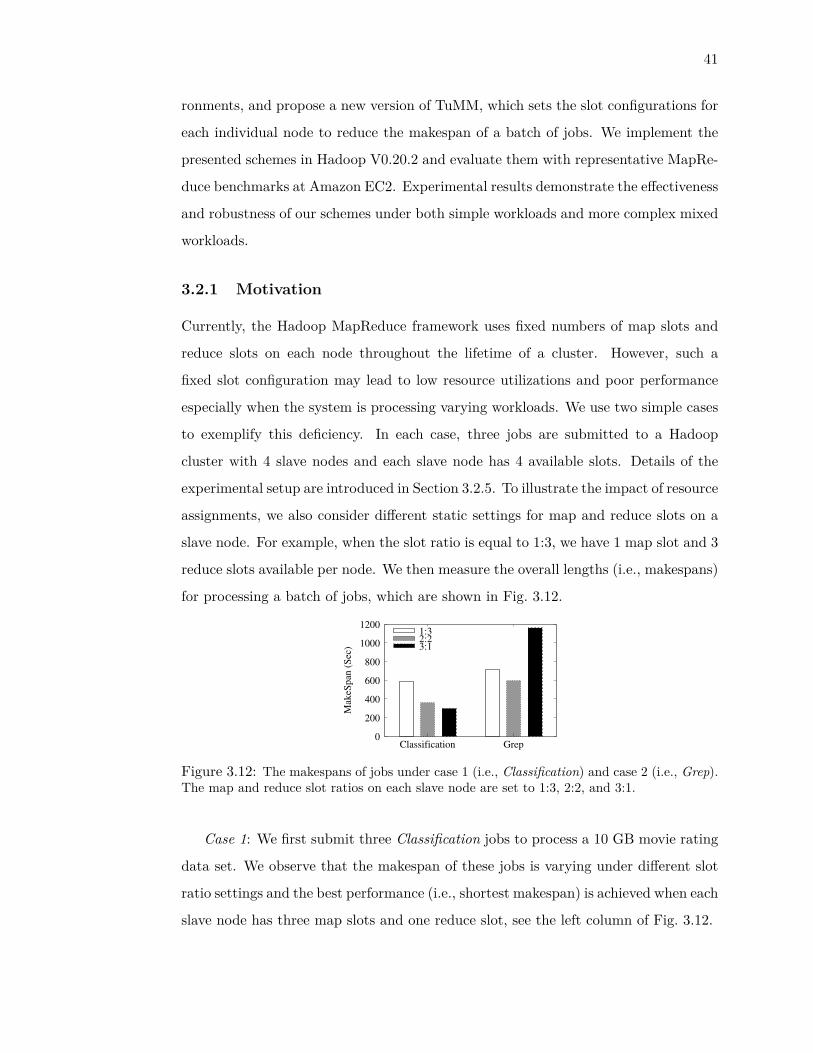
41

ronments, and propose a new version of TuMM, which sets the slot configurations for

each individual node to reduce the makespan of a batch of jobs. We implement the

presented schemes in Hadoop V0.20.2 and evaluate them with representative MapRe-

duce benchmarks at Amazon EC2. Experimental results demonstrate the effectiveness

and robustness of our schemes under both simple workloads and more complex mixed

workloads.

3.2.1 Motivation

Currently, the Hadoop MapReduce framework uses fixed numbers of map slots and

reduce slots on each node throughout the lifetime of a cluster. However, such a

fixed slot configuration may lead to low resource utilizations and poor performance

especially when the system is processing varying workloads. We use two simple cases

to exemplify this deficiency. In each case, three jobs are submitted to a Hadoop

cluster with 4 slave nodes and each slave node has 4 available slots. Details of the

experimental setup are introduced in Section 3.2.5. To illustrate the impact of resource

assignments, we also consider different static settings for map and reduce slots on a

slave node. For example, when the slot ratio is equal to 1:3, we have 1 map slot and 3

reduce slots available per node. We then measure the overall lengths (i.e., makespans)

for processing a batch of jobs, which are shown in Fig. 3.12.

1:32:23:1

0

200

400

600

800

1000

1200

Classification Grep

Mak

eSp

an (

Sec

)

Figure 3.12: The makespans of jobs under case 1 (i.e., Classification) and case 2 (i.e., Grep).The map and reduce slot ratios on each slave node are set to 1:3, 2:2, and 3:1.

Case 1: We first submit three Classification jobs to process a 10 GB movie rating

data set. We observe that the makespan of these jobs is varying under different slot

ratio settings and the best performance (i.e., shortest makespan) is achieved when each

slave node has three map slots and one reduce slot, see the left column of Fig. 3.12.

42

0 2 4 6 8

10 12 14 16 18

0 100 200 300

Slo

t

Time (Sec)

(a) 2 map slots : 2 reduce slots

0 2 4 6 8

10 12 14 16 18

0 100 200 300

Slo

t

Time (Sec)

(b) 3 map slots : 1 reduce slot

Figure 3.13: Task execution times of three Classification jobs under different static slotconfigurations, where each node has (a) 2 map slots and 2 reduce slots, and (b) 3 map slotsand 1 reduce slot. Each arrowed line represents the execution of one task, and the solid (resp.dashed) ones represent map (resp. reduce) tasks. The first wave in each job’s reduce phaserepresents the shuffle operations. In addition, we use three different colors to discriminate thethree jobs.

To interpret this effect, we further plot the execution times of each task in Fig. 3.13.

Clearly, Classification is a map-intensive application; for example, when we equally

distribute resources (or slots) between map and reduce tasks, i.e., with the slot ratio

of 2:2, the length of a map phase is longer than that of a reduce phase, see Fig. 3.13(a).

It follows that each job’s reduce phase (including shuffle operations and reduce op-

erations) overlaps with its map phase for a long period. However, as the reduce

operations can only start after the end of the map phase, the occupied reduce slots

stay in shuffle for a long period, mainly waiting for the outputs from the map tasks.

Consequently, system resources are underutilized.

For example, we tracked the cpu utilizations of each task in a slave node every 5

seconds and Table 3.10 shows part of the records in one of such overlapping periods.

At each moment, the overall cpu utilization (i.e., the summation of cpu utilizations

of the four tasks) is much less than 400%, for a node with 4 cores. We then notice

that when we assign more slots to map tasks, e.g., with the slot ratio of 3:1, each

job experiences a shorter map phase and most of its reduce phase overlaps with

the following job’s map phase, see Fig. 3.13(b). The average cpu utilization is also

43

increased by 20% comparing to those under the the slot ratio of 2:2. It implies that

for map-intensive jobs like Classification, one should assign more resources (slots) to

map tasks in order to improve the performance in terms of makespan.

Table 3.10: Real time CPU utilizations of each task on a slave node in the overlapping timeperiod of a job’s map and reduce phases. The slot ratio per node is 2:2.

ProcessId/TaskTypeTime(sec) 3522/map 3564/map 3438/reduce 3397/reduce

1 147% 109% 26% 0%6 103% 93% 0% 4%11 93% 99% 8% 0%16 100% 100% 0% 0%21 97% 103% 0% 0%

Case 2: In this case, we turn to consider reduce-intensive applications by submit-

ting three Grep jobs to scan the 10 GB movie rating data. Similar to case 1, we also

investigate three static slot configurations.

First, we observe that each job takes longer time to process its reduce phase than

its map phase when we have 2 map and 2 reduce slots per node, see Fig. 3.14(a).

Based on the observation in case 1, we expect a reduced makespan when assigning

more slots to reduce tasks, e.g., with the slot ratio of 1:3. However, the experimental

results show that the makespan under this slot ratio setting (1:3) becomes even longer

than that under the setting of 2:2, see the right column of Fig. 3.12. We then look

closely at the corresponding task execution times, see Fig. 3.14(b). We find that the

reduce tasks indeed have excess slots such that the reduce phase of each job starts

too early and wastes time waiting for the output from its map phase. In fact, a good

slot ratio should be set between 2:2 and 1:3 to enable each job’s reduce phase to fully

overlap with the following job’s map phase rather than its own map phase.

In summary, in order to reduce the makespan of a batch of jobs, more resources (or

slots) should be assigned to map (resp. reduce) tasks if we have map (resp. reduce)

intensive jobs. On the other hand, a simple adjustment in such slot configurations

is not enough. An effective approach should tune the slot assignments such that the

execution times of map and reduce phases can be well balanced and the makespan of

a given set can be reduced to the end.

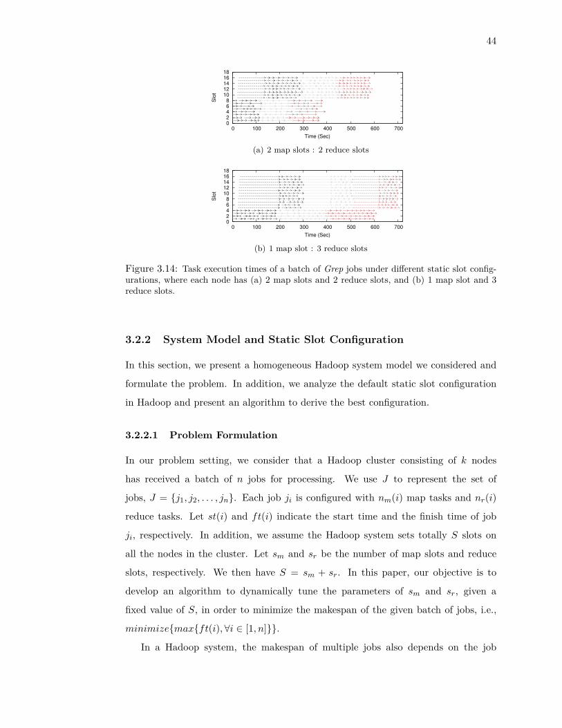
44

0 2 4 6 8

10 12 14 16 18

0 100 200 300 400 500 600 700

Slo

t

Time (Sec)

(a) 2 map slots : 2 reduce slots

0 2 4 6 8

10 12 14 16 18

0 100 200 300 400 500 600 700

Slo

t

Time (Sec)

(b) 1 map slot : 3 reduce slots

Figure 3.14: Task execution times of a batch of Grep jobs under different static slot config-urations, where each node has (a) 2 map slots and 2 reduce slots, and (b) 1 map slot and 3reduce slots.

3.2.2 System Model and Static Slot Configuration

In this section, we present a homogeneous Hadoop system model we considered and

formulate the problem. In addition, we analyze the default static slot configuration

in Hadoop and present an algorithm to derive the best configuration.

3.2.2.1 Problem Formulation

In our problem setting, we consider that a Hadoop cluster consisting of k nodes

has received a batch of n jobs for processing. We use J to represent the set of

jobs, J = {j1, j2, . . . , jn}. Each job ji is configured with nm(i) map tasks and nr(i)

reduce tasks. Let st(i) and ft(i) indicate the start time and the finish time of job

ji, respectively. In addition, we assume the Hadoop system sets totally S slots on

all the nodes in the cluster. Let sm and sr be the number of map slots and reduce

slots, respectively. We then have S = sm + sr. In this paper, our objective is to

develop an algorithm to dynamically tune the parameters of sm and sr, given a

fixed value of S, in order to minimize the makespan of the given batch of jobs, i.e.,

minimize{max{ft(i), ∀i ∈ [1, n]}}.

In a Hadoop system, the makespan of multiple jobs also depends on the job

45

scheduling algorithm which is coupled with our solution of allocating the map and

reduce slots on each node. In this paper, we assume that a Hadoop cluster uses the

default FIFO (First-In-First-Out) job scheduler because of the following two reasons.

First, given n jobs waiting for service, the performance of FIFO is no worse than Fair

in terms of makespan. In the example of “Case 2” mentioned in Section 3.2.1, the

makespan under FIFO is 594 sec while Fair, another alternative scheduler in Hadoop,

consumes 772 sec to finish jobs. Second, using FIFO simplifies the performance analy-

sis because generally speaking, there are fewer concurrently running jobs at any time.

Usually two jobs, with one in map phase and the other in reduce phase.

Furthermore, we use execution time to represent the workload of each job. As a

MapReduce job is composed of two phases, we define wm(i) and wr(i) as the workload

of map phase and reduce phase in job ji, respectively. We have developed solutions

with and without the prior knowledge of the workload and we will discuss how to

obtain this information later.

3.2.2.2 Static Slot Configuration with Workload Information

First, we consider the scenario that the workload of a job is available and present the

algorithm for static slot configuration which is default in a Hadoop system. Basically,

the Hadoop cluster preset the values of sm and sr under the constraint of S = sm+sr

before executing the batch of jobs, and the slot assignment will not be changed during

the entire process. We have developed the following Algorithm 3.4 to derive the

optimal values of sm and sr.

Our algorithm and analysis are based on an assumption that the time needed to

finish the workload of map or reduce phase is inversely proportional to the number

of slots assigned to the phase in a homogeneous Hadoop cluster. Given sm and sr,

the map (resp. reduce) phase of ji needs nm(i)sm

(resp. nr(i)sr

) rounds to finish. In

each round, sm map tasks or sr reduce tasks are processed in parallel and the time

consumed is equal to the execution time of one map or one reduce task. Let tm(i) and

tr(i) be the average execution time for a map task and a reduce task, respectively.

The workloads of map and reduce phases are defined as

wm(i) = nm(i) · tm(i), wr(i) = nr(i) · tr(i). (3.9)

46

Algorithm 3.4 can derive the best static setting of sm and sr given the workload

information. The outer loop (lines 1–10) in the algorithm enumerates the value of smand sr (i.e., S − sm). For each setting of sm and sr, the algorithm first calculates

the workload (wm(i) and wr(i)) for each job ji in lines 3–5. The second inner loop

(lines 6–8) is to calculate the finish time of each job. Under the FIFO policy, there

are at most two concurrently running jobs in the Hadoop cluster. Each job’s map or

reduce phase cannot start before the precedent job’s map or reduce phase is finished

(we assume here that all jobs have more tasks than the slots number in system for

the simplicity of discussion). More specifically, the start time of map tasks of job

ji, i.e., st(i), is the finish time of ji−1’s map phase, i.e., st(i) = st(i − 1) + wm(i−1)sm

.

Additionally, the start time of ji’s reduce phase should be no earlier than both the

finish time of ji’s map phase and the finish time of ji−1’s reduce phase. Therefore, the

finish time of ji is ft(i) = max(st(i) + wm(i)sm

, ft(i− 1)) + wr(i)sr

. Finally, the variables

Opt SM and Opt MS keep track of the optimal value of sm and the corresponding

makespan (lines 9–10), and the algorithm returns Opt SM and S − Opt SM as the

values for sm and sr at the end. The time complexity of the algorithm is O(S · n).

Algorithm 3.4 Static Slot Configuration1: for sm = 1 to S do2: sr = S − sm

3: for i = 1 to n do4: wm(i) = nm(i) · tm(i)5: wr(i) = nr(i) · tr(i)6: end for7: for i = 1 to n do8: st(i) = st(i− 1) + wm(i−1)

sm

9: ft(i) = max(st(i) + wm(i)sm

, ft(i− 1)) + wr(i)sr

10: end for11: if ft(n) < Opt MS then12: Opt MS = ft(n); Opt SM = sm

13: end if14: end for15: return Opt SM and S −Opt SM

3.2.3 Dynamic Slot Configuration Under Homogeneous

Environments

As discussed in Section 3.2.1, the default Hadoop cluster uses static slot configuration

and does not perform well for varying workloads. The inappropriate setting of sm

47

and sr may lead to extra overhead because of the following two cases:

(1) if job ji’s map phase is completed later than job ji−1’s reduce phase, then the

reduce slots will be idle for the interval period of (st(i) + wm(i)) − ft(i − 1), see

Fig. 3.15(a);

(2) if job ji’s map phase is completed earlier than the job ji−1’s reduce phase, then

ji’s reduce tasks have to wait for a period of ft(i− 1)− (st(i) + wm(i)) until reduce

slots are released by ji−1, see Fig. 3.15(b).

job i

job i-1 job i

job i

job i-1 job i

job i

job i-1 job i

Map

Reduce

(a) (b) (c)

Figure 3.15: Illustration of aligning the map and reduce phases. (a) and (b) are the twoundesired cases mentioned above, and our goal is to achieve (c).

In this section, we present our solutions that dynamically allocate the slots to

map and reduce tasks during the execution of jobs. The architecture of our design is

shown in Fig. 3.16. In dynamic slot configuration, when one slot becomes available

upon the completion of a map or reduce task, the Hadoop system will re-assign a

map or reduce task to the slot based on the current optimal values of sm and sr.

There are totally∑i∈[1,n](nm(i) + nr(i)) tasks and at the end of each task, Hadoop

needs to decide the role of the available slot (either a map slot or a reduce slot).

In this setting, therefore, we cannot enumerate all the possible values of sm and

sr (i.e., 2∑

i(nm(i)+nr(i)) combinations) as in Algorithm 3.4. Instead, we modify our

objective in the dynamic slot configuration as there is no closed-form expression of

the makespan.

Our goal now is, for the two concurrently running jobs (one in map phase and

the other in reduce phase), to minimize the completion time of these two phases.

Our intuition is to eliminate the two undesired cases mentioned above by aligning

the completion of ji’s map phase and ji−1’s reduce phase, see Fig. 3.15(c). Briefly,

we use the slot assignment as a tunable knob to change the level of parallelism of

map or reduce tasks. When we assign more map slots, map tasks obtain more system

resources and could be finished faster, and vice versa for reduce tasks. In the rest of

this section, we first present our basic solution with the assumption of prior knowledge

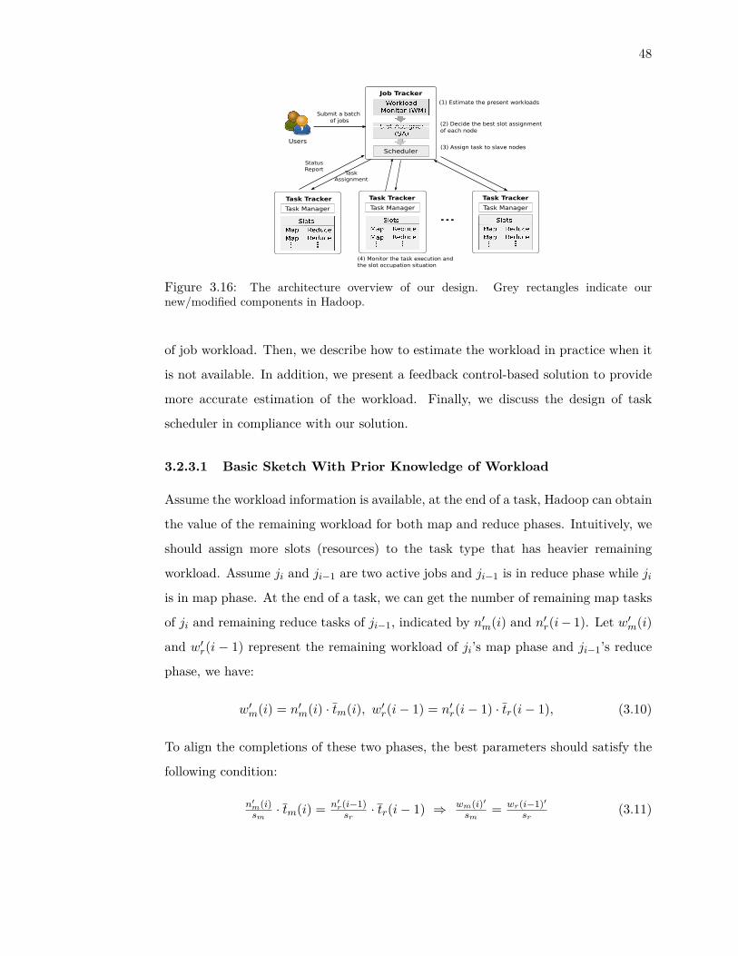
48

Job Tracker

Scheduler

Task Tracker

Task Manager

Task Tracker

Task Manager

Task Tracker

Task Manager

...

Submit a batch

of jobs

Status

ReportTask

Assignment

Users

(1) Estimate the present workloads

(2) Decide the best slot assignment

of each node

(3) Assign task to slave nodes

(4) Monitor the task execution and

the slot occupation situation

Figure 3.16: The architecture overview of our design. Grey rectangles indicate ournew/modified components in Hadoop.

of job workload. Then, we describe how to estimate the workload in practice when it

is not available. In addition, we present a feedback control-based solution to provide

more accurate estimation of the workload. Finally, we discuss the design of task

scheduler in compliance with our solution.

3.2.3.1 Basic Sketch With Prior Knowledge of Workload

Assume the workload information is available, at the end of a task, Hadoop can obtain

the value of the remaining workload for both map and reduce phases. Intuitively, we

should assign more slots (resources) to the task type that has heavier remaining

workload. Assume ji and ji−1 are two active jobs and ji−1 is in reduce phase while jiis in map phase. At the end of a task, we can get the number of remaining map tasks

of ji and remaining reduce tasks of ji−1, indicated by n′m(i) and n′r(i− 1). Let w′m(i)

and w′r(i − 1) represent the remaining workload of ji’s map phase and ji−1’s reduce

phase, we have:

w′m(i) = n′m(i) · tm(i), w′r(i− 1) = n′r(i− 1) · tr(i− 1), (3.10)

To align the completions of these two phases, the best parameters should satisfy the

following condition:

n′m(i)sm· tm(i) = n′r(i−1)

sr· tr(i− 1) ⇒ wm(i)′

sm= wr(i−1)′

sr(3.11)

49

Therefore, the number of map and reduce slots should be proportional to their re-

maining workloads as shown in Eq. 3.12-3.13,

sm = b w′m(i)w′m(i) + w′r(i− 1) · Sc, (3.12)

sr = S − sm, (3.13)

where sm and sr represent the target numbers of map and reduce slots respectively,

and S is the total number of slots in the cluster which is configured based on system

capacity. Furthermore, we introduce the upper bound shm and the lower bound slm for

the map slots assignment. When the estimated value of sm exceeds the bounds, we

use the bound value as the new sm value instead. In our design, slm is set to be the

number of nodes in the cluster (k) such that there is at least one map slot on each

node at any time. Similarly, shm is set to be equal to S−slm such that the reduce slots

number in each node is always greater than or equal to 1. When a map or reduce

task is finished, one slot becomes available. The Hadoop system calculates the values

of sm and sr according to Eq. 3.12-3.13. If the current map slots are fewer than sm,

then the available slot will become a map slot and serve a map task. Otherwise, it

turns to a reduce slot. With this setting, the current map and reduce phases could

finish at approximately the same time with a high system resource utilization.

3.2.3.2 Workload Estimation

Our solution proposed above depends on the assumption of prior knowledge of work-

load information. In practice, workload can be derived from job profiles, training

phase, or other empirical settings. In some applications, however, workload informa-

tion may not be available or accurate. In this subsection, we present a method that

estimates the workload during the job execution without any prior knowledge.

We use w′m and w′r to represent the remaining workload of a map or reduce

phase, i.e., the summation of execution time of the unfinished map or reduce tasks.

Note that we only track the map/reduce workloads of running jobs, but not the jobs

waiting in the queue. Basically, the workload is calculated as the production of the

number of remaining tasks and the average task execution time of a job. Specifically,

when a map or reduce task is finished, the current workload information needs to be

updated, as shown in Algorithm 3.5, where n′m(i)/ n′r(i) is the number of unfinished

50

map/reduce tasks of job ji, and tm(i)/ tr(i) means the average execution time of

finished map/reduce tasks from ji. Note that the execution time of each finished

task is already collected and reported to the JobTracker in current Hadoop systems.

In addition, we use Welford’s one pass algorithm to calculate the average of task

execution times, which incurs very low overheads on both time and memory space.

Algorithm 3.5 Workload Information Collectorif a map task of job ji is finished then

update the average execution time of a map task tm(i)w′m(i) = tm(i) · n′m(i)

end ifif a reduce task of job ji is finished then

update the average execution time of a reduce task tr(i)w′r(i) = tr(i) · n′r(i)

end if

3.2.3.3 Feedback Control-based Workload Estimation

In this subsection, we present an enhanced workload estimation algorithm to achieve

more accurate workload information. Our previous analysis adopts an assumption

that the execution time of a map or reduce task is similar, represented by the average

values tm(i) and tr(i), respectively. They are also used for calculating the workload

wm and wr. This estimation works well in systems where the slots assignment is

fixed. In our system design, however, the slots assignment is dynamically changed,

which affects the per task execution time in practice. Assigning more slots to one

type of tasks may cause the contention on a particular system resource and lead to

an increased execution time of each following task in the same type. For example,

in “Case 2” described in Section 3.2.1, when we use 1 map slot on each node, the

average execution time of a map task is 18.5 sec. When we increase the number of

map slots per node to 2, the average execution time of a map task becomes 23.1 sec

with a 25% increase.

To overcome this issue, we have designed a feedback control based mechanism

to tune the slots assignment. Under this mechanism, the slots assignment, sm and

sr, is first calculated through Eq. 3.12-3.13. An additional routine is introduced to

periodically update the workload information based on newly captured average task

execution times. If the workloads have changed, then the slots assignment will also

51

be updated according to Eq. 3.14-3.15.

sm = sm + bα · ( w′mw′m + w′r

− wmwm + wr

) · Sc, (3.14)

sr = S − sm. (3.15)

When the new estimated workloads, i.e., w′m and w′r, differ from the previous

estimation, an integral gain parameter α is used to control the new assignment of

slots based on the new estimation. The Hadoop system will iteratively calculate smand sr (Eq. 3.14-3.15) until there is no change on these two parameters. The value of

α is set to be 1.2 in our system such that the slots assignment could converge quickly.

3.2.3.4 Slot Assigner

The task assignment in Hadoop works in a heartbeat fashion: the TaskTrackers re-

port slots occupation situation to the JobTracker with heartbeat messages; and the

JobTracker selects tasks from the queue and assigns them to free slots. There are

two new problems need to be addressed when assigning tasks under TuMM. First,

slots of each type should be evenly distributed across the slave nodes. For example,

when we have a new slot assignment sm = 5, sr = 7 in a cluster with 2 slave nodes,

a 2:3/4:3 map/reduce slots distribution is better than the 1:4/5:2 map/reduce slots

distribution in case of resource contention. Second, the currently running tasks may

stick with their slots and therefore the new slot assignments may not be able to apply

immediately. To address these problems, our slot assignment module (SA) takes both

the slots assignment calculated through Eq. 3.14-3.15 and the situation of currently

running tasks into consideration when assigning tasks.

The process of SA is shown in Algorithm 3.6. The SA first calculates the map

and reduce slot assignments of slave node x (line 1), indicated by sm(x) and sr(x),

based on the current values of sm and sr and the number of running tasks in cluster.

Because of the flooring operation in line 1, the assigned slots (sm(x) + sr(x)) on node

x may be fewer than the available slots (S/k). In lines 3–6, we increase either sm(x)

or sr(x) to compensate slot assignment. Our decision is based on the deficit of current

map and reduce slots (line 3), where sm/ sr represent our target assignment and rtm/

rtr are the number of current running map/reduce tasks. Eventually, we assign a

task to the available slot in lines 7–10. Similarly, the decision is made by comparing

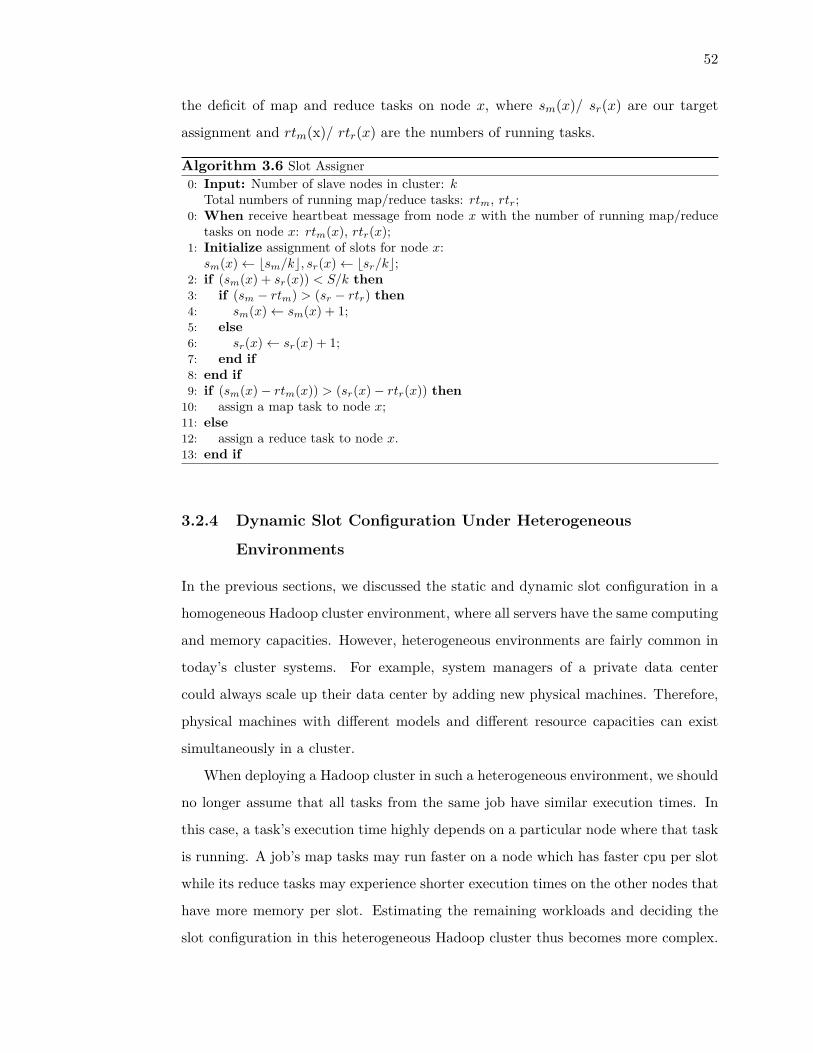
52

the deficit of map and reduce tasks on node x, where sm(x)/ sr(x) are our target

assignment and rtm(x)/ rtr(x) are the numbers of running tasks.

Algorithm 3.6 Slot Assigner0: Input: Number of slave nodes in cluster: k

Total numbers of running map/reduce tasks: rtm, rtr;0: When receive heartbeat message from node x with the number of running map/reduce

tasks on node x: rtm(x), rtr(x);1: Initialize assignment of slots for node x:sm(x)← bsm/kc, sr(x)← bsr/kc;

2: if (sm(x) + sr(x)) < S/k then3: if (sm − rtm) > (sr − rtr) then4: sm(x)← sm(x) + 1;5: else6: sr(x)← sr(x) + 1;7: end if8: end if9: if (sm(x)− rtm(x)) > (sr(x)− rtr(x)) then

10: assign a map task to node x;11: else12: assign a reduce task to node x.13: end if

3.2.4 Dynamic Slot Configuration Under Heterogeneous

Environments

In the previous sections, we discussed the static and dynamic slot configuration in a

homogeneous Hadoop cluster environment, where all servers have the same computing

and memory capacities. However, heterogeneous environments are fairly common in

today’s cluster systems. For example, system managers of a private data center

could always scale up their data center by adding new physical machines. Therefore,

physical machines with different models and different resource capacities can exist

simultaneously in a cluster.

When deploying a Hadoop cluster in such a heterogeneous environment, we should

no longer assume that all tasks from the same job have similar execution times. In

this case, a task’s execution time highly depends on a particular node where that task

is running. A job’s map tasks may run faster on a node which has faster cpu per slot

while its reduce tasks may experience shorter execution times on the other nodes that

have more memory per slot. Estimating the remaining workloads and deciding the

slot configuration in this heterogeneous Hadoop cluster thus becomes more complex.

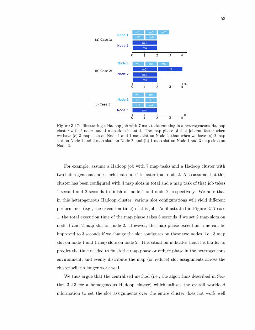
53

Node 1

Node 2

0 2 4

m3

m2

m1 m5

m6

m7

m4

31

Node 1

Node 2

0 2 4

m3

m1 m5 m6

m4

31

m2 m7

Node 1

Node 2

0 2 4

m3

m1 m5

m4

31

m2m2

m3

m6

m7

(a) Case 1:

(b) Case 2:

(c) Case 3:

Figure 3.17: Illustrating a Hadoop job with 7 map tasks running in a heterogeneous Hadoopcluster with 2 nodes and 4 map slots in total. The map phase of that job run faster whenwe have (c) 3 map slots on Node 1 and 1 map slot on Node 2, than when we have (a) 2 mapslot on Node 1 and 2 map slots on Node 2, and (b) 1 map slot on Node 1 and 3 map slots onNode 2.

For example, assume a Hadoop job with 7 map tasks and a Hadoop cluster with

two heterogeneous nodes such that node 1 is faster than node 2. Also assume that this

cluster has been configured with 4 map slots in total and a map task of that job takes

1 second and 2 seconds to finish on node 1 and node 2, respectively. We note that

in this heterogeneous Hadoop cluster, various slot configurations will yield different

performance (e.g., the execution time) of this job. As illustrated in Figure 3.17 case

1, the total execution time of the map phase takes 3 seconds if we set 2 map slots on

node 1 and 2 map slot on node 2. However, the map phase execution time can be

improved to 3 seconds if we change the slot configures on these two nodes, i.e., 3 map

slot on node 1 and 1 map slots on node 2. This situation indicates that it is harder to

predict the time needed to finish the map phase or reduce phase in the heterogeneous

environment, and evenly distribute the map (or reduce) slot assignments across the

cluster will no longer work well.

We thus argue that the centralized method (i.e., the algorithms described in Sec-

tion 3.2.3 for a homogeneous Hadoop cluster) which utilizes the overall workload

information to set the slot assignments over the entire cluster does not work well

54

any more when the nodes in the cluster become heterogenous. Motivated by this, we

present in this section a new version of TuMM, named H TuMM, which dynamically

sets the slot configurations for each node in a heterogeneous Hadoop cluster in order

to reduce the makespan of a batch of Hadoop jobs.

3.2.4.1 Problem Formulation

The problem of finding the optimal slot assignment to map and reduce tasks in a het-

erogeneous Hadoop cluster that aligns the current running map and reduce workloads

and minimizes the time required to finish current map and reduce workloads could

be formulated as a linear programming problem as follows:

Minimize max {vim ∗ tim},∀i ∈ I, (3.16)

subject to :

sim + sir = Si, ∀i ∈ I, (3.17)∑vim ∗ sim >= n′m, ∀i ∈ I, (3.18)∑vir ∗ sir >= n′r, ∀i ∈ I, (3.19)

(vjm − 1) ∗ tjm <= vim ∗ tim,

∀i, j ∈ I, if tim < tjm, (3.20)

vim ∗ tim <= (vjm + 1) ∗ tjm,

∀i, j ∈ I, if tim < tjm. (3.21)

(vjr − 1) ∗ tjr <= vir ∗ tir,

∀i, j ∈ I, if tir < tjr, (3.22)

vir ∗ tir <= (vjr + 1) ∗ tjr,

∀i, j ∈ I, if tir < tjr. (3.23)

(vjr − 1) ∗ tjr <= vim ∗ tim,

∀i, j ∈ I, if tim < tjr, (3.24)

vim ∗ tim <= (vjr + 1) ∗ tjr,

∀i, j ∈ I, if tim < tjr, (3.25)

Here, I represents the set of nodes in the cluster, tim/tir represents the average

map/reduce task execution time on node i, and n′m/n′r represents the remaining unas-

55

signed map/reduce tasks of jobs that are currently running under their map/reduce

phases. Additionally, vim/vir denotes the waves of map/reduce tasks that have to run

on node i before the finish time of current map/reduce phase, sim/sir represents the

optimal slot assignment to map/reduce on node i, and Si represents the constraint

of total avaliable slot number of node i. The target is to minimize the finish time

of the current map phase under a set of constraints: Eq.(3.17) states that the slots

assigned to map or reduce tasks on each node should not exceed the pre-defined slot

constraint of that particular node; Eq.s(3.18)-(3.19) state that all the remaining tasks

of current running jobs need to be assigned across the cluster; Eq.s(3.20)-(3.21) state

that the difference between the times each node takes to execute its assigned map

tasks should not exceed the execution time of one task (this constraint is decided by

the nature of the Hadoop scheduler); Eq.s(3.22)-(3.23), similarly, state that the time

each node taskes to execute its assigned reduce tasks should be roughly the same;

and Eq.s(3.24)-(3.25) state that the finish time of map and reduce workloads that are

dispatched to each node should also be aligned to avoid slot idleness.

However, the time complexity to solve the above problem is extremely high. In

order to make decisions for slot configurations instantly when the workloads change,

we instead present a new algorithm which solves the problem by heuristically assigning

slots for map and reduce tasks on each node in a heterogeneous Hadoop cluster.

3.2.4.2 Algorithm Design: H TuMM

H TuMM shares the similar idea of TuMM, i.e., dynamically assign slots to map and

reduce tasks to align the process of map and reduce phase based on the collected

workload information. The key difference of H TuMM is to set the slot configurations

for each node individually in a heterogeneous cluster, i.e., each of those nodes will

have different slot assignment ratio between map and reduce tasks.

To accomplish it, H TuMM collects the workload information on the entire cluster

and on each individual node as well: when a map/reduce task is finished on node i,

the workload collector updates (1) the average execution time of map/reduce tasks,

i.e., tm/tr; and (2) the average execution of map/reduce tasks that ran on node i, i.e.,

tim/tir.

Based on the collected workload information, H TuMM performs slot assignment

56

for each node as shown in Algorithm 3.7. Once a slot in node i becomes available,

H TuMM first updates the slot assignments to map tasks (sim) and reduce tasks (sir)

on node i. Such that the ratio of slot assignments (i.e., sim/sir) is equal to the ratio

of remaining map and reduce workloads (i.e., tim∗n′mtir∗n′r

, see line 1-2 in Algorithm 3.7.

Therefore, map and reduce phases running on that node are aligned. Similar to

Algorithm 3.6, floor function is used to make sure that slots assignments are all

integers. If there is one remaining slot, in this case, the free slot will be assigned to

a map (resp. reduce) task if map (resp. reduce) tasks run relatively faster on this

node compared to the average execution time across the entire cluster in order to

improve the efficiency, see line 3-7 in Algorithm 3.7. When the slot assignment on the

specific node is determined, the JobTracker can assign tasks based on the new slot

configuration and the number of currently running tasks on that node (i.e., rtim and

rtir), see line 8-11 in Algorithm 3.7.

Algorithm 3.7 Slot Assignment for Node i0: Input: Average task execution time on node i and across the cluster, and the remaining

task number of current running jobs;0: When Node i has free slots and ask for new task assignment through the heartbeat

message;1: si

m ← bSi ∗ tim∗n

′m

tim∗n′m+ti

r∗n′rc;

2: sir ← bSi ∗ ti

r∗n′r

tim∗n′m+ti

r∗n′rc;

3: if sim + si

r < Si then4: if ti

m

tm>

tir

trthen

5: sir ← Si − si

m;6: else7: si

m ← Si − sir.

8: end if9: end if

10: if (sim − rtim) > (si

r − rtir) then11: assign a map task to node i;12: else13: assign a reduce task to node i;14: end if

3.2.5 Evaluation

3.2.5.1 Experimental Setup and Workloads

Implementation We implemented our new scheme (for homogeneous environment

and heterogeneous environment) on top of Hadoop Version 0.20.2. First, we added

57

two new modules to the JobTracker: the Workload Monitor (WM) that is responsible

to collect past workload information such as execution times of completed tasks and

to estimate the workloads of currently running map and reduce tasks and the Slot

Assigner (SA) which uses the estimated information received from WM to adjust the

slot ratio between map and reduce for each slave node. The JobTracker with these

additional modules will then assign tasks to a slave node based on the adjusted slot

ratio and the current slot status at that particular node. In addition, we modified

the TaskTracker as well as the JvmManager running on each slave node to check

the number of individual map and reduce tasks running on that node based on the

new slot ratio received from the JobTracker. The architecture overview of this new

Hadoop framework is shown in Fig. 3.16.

Benchmarks We choose five representative data-analyzing Hadoop benchmarks

from Purdue MapReduce Benchmarks Suite [32]:

• Inverted Index: input text documents and generate word to document indexing.

• Histogram Rating: input the movie rating data and calculate the histogram.

• Word Count: take text documents as input and count the occurrence of each

word.

• Classification: take the movie rate data and classify movies into predefined

clusters.

• Grep: input text documents and search for a pattern in the files.

In addition, we use different sizes of movie rating data [32] that consists of user

ranking information and wiki category links data [33] that includes the information

about wiki page categories, as the input to the above five benchmarks. A 10GB movie

rating data and a 7GB wiki category data are used as input for experiments in the

homogeneous cluster. And experiments under the heterogeneous cluster use a 8GB

movie rating data and a 8GB wiki category data as inputs.

We further choose TPC-H [34] queries expressed as Pig programs [35] to validate

the performance of H TuMM under heterogeneous environments. A data generator in

TPC-H can be used to create a database with the customized size. In such a database,

58

there are totally eight tables, i.e., customer, supplier, orders, lineitem, part, partsupp,

nation, and region. In our experiments, we generated a database with 4G data in total

and selected three queries from the TPC-H benchmark to evaluate the performance

of H TuMM.

• TPCH-Q15: This query finds the supplier who contributed the most to the

overall revenue for parts shipped during a given quarter of a given year.

• TPCH-Q16: This query counts the number of suppliers who can supply parts

that satisfy a particular customer’s requirements.

• TPCH-Q18: This query finds a list of the top 100 customers who have ever

placed large quantity orders.The query lists the customer name, customer key,

the order key, date and total price and the quantity for the order.

3.2.5.2 Performance Evaluation in Homogeneous Environment

In this section, we evaluate the performance of TuMM in terms of the makespan of

a batch of MapReduce jobs in a homogeneous environment. we launch a Hadoop

cluster in the Amazon EC2 environment which consists of 5 m1.xlarge Amazon EC2

instances. Specifically, we have one master node and four slave nodes in the cluster.

The number of slots which can be available on each slave node is set as 4 since an

m1.xlarge instance at Amazon EC2 has 4 virtual cores.

We first consider the simple workloads which consist of jobs from a single MapRe-

duce benchmark and then validate the robustness of our approach with a mixed

workload that is a combination of different MapReduce benchmarks from Purdue

MapReduce Benchmarks Suite.

Simple Workloads We here conduct a set of experiments such that in each

experiment 3 Hadoop jobs from one of the above benchmarks (see Section 3.2.5.1)

are waiting for service. We remark that such a simple workload is often found in real

systems as the same Hadoop jobs may be executed repeatedly to process similar or

different input data sets. In our experiments, three Hadoop jobs use the same data set

as the input. Furthermore, as the comparisons, we evaluate the performance under

the static slot ratios for map and reduce. With our setting in the evaluation (i.e., total

number of slots per node is 4), we consider three static configuration alternatives, i.e.,

59

1:3, 2:2 and 3:1, for a Hadoop cluster. We enumerate all these three possible settings

for the comparison with our solution.

TuMM TuMM TuMM

TuMM TuMM

1:3 2:2 3:1 1:3 2:2 3:1 1:3 2:2 3:1

1:3 2:2 3:1 1:3 2:2 3:1 0

100

200

300

400

500

600

Mak

eSpan

(S

ec)

0

200

400

600

800

1000

1200

Mak

eSpan

(S

ec)

(d) Classification (e) Grep

0

500

1000

1500

2000

2500

3000

3500

Mak

eSpan

(S

ec)

0

200

400

600

800

1000

1200

1400

1600

1800

Mak

eSpan

(S

ec)

0

200

400

600

800

1000

1200

1400

Mak

eSpan

(S

ec)

(c) Word Count(b) Histogram Rating(a) Inverted Index

Figure 3.18: Makespans of five Hadoop applications under TuMM and three static slotconfigurations.

Fig. 3.18 shows the makespans (i.e., the completion lengths) of a given set when we

have different slot configurations. We first observe that the performance varies a lot

under three static slot settings. For example, the Inverted Index jobs experience the

fastest makespan when the slot ratio is equal to 1:3. In contrast, the Histogram Rating

jobs achieve better performance when we assign more slots to their map tasks, e.g.,

with slot ratio of 3:1. We also observe that TuMM always yields the best performance,

i.e., the shortest makespan, for all the five Hadoop benchmarks. We interpret this

effect as the result of dynamic slot ratio adjustments enabled by TuMM.

Compared to the slot ratio of 2:2, our approach in average achieves about 20%

relative improvement in the makespan. Moreover, such improvement becomes more

visible when the workloads of map and reduce tasks become more unbalanced. For

example, the makespan of the Inverted Index jobs is reduced by 28% where these jobs

have their reduce phases longer than their map phases.

Mixed Workloads In the previous experiments, each workload only contains jobs

from the same benchmark. Now, we consider a more complex workload, which mixes

jobs from different Hadoop benchmarks. Reducing the makespan for such a mixed

workload thus becomes non-trivial. One solution to tackle this problem is to shuffle

the execution order of these jobs. For example, the classic Johnson’s algorithm [36]

that was proposed for building an optimal two-stage job schedule, could be applied

60

0

5

10

15

20

25

0 300 600 900 1200 1500 1800 2100 2400

Slo

t

Time (Sec)

(a) Johnson’s Algorithm

(1)

0

5

10

15

20

25

0 300 600 900 1200 1500 1800 2100 2400

Slo

t

Time (Sec)

(b) Reversed Johnson’s Algorithm

(3)

0

5

10

15

20

25

0 300 600 900 1200 1500 1800 2100 2400

Slo

t

Time (Sec)

(c) Random Sequence

(5)

0 2 4 6 8

10 12 14 16

0 500 1000 1500 2000

Slo

ts N

um

be

r

Time (Sec)(2)

Map SlotsReduce Slots

0 2 4 6 8

10 12 14 16

0 500 1000 1500 2000

Slo

ts N

um

be

r

Time (Sec)(4)

Map SlotsReduce Slots

0 2 4 6 8

10 12 14 16

0 500 1000 1500 2000

Slo

ts N

um

be

r

Time (Sec)(6)

Map SlotsReduce Slots

Figure 3.19: Illustrating task execution times and slot assignments across time under TuMM,where the job execution sequence is (a) generated by Johnson’s algorithm; (b) inverse to thefirst one; and (c) random. In the plots at the second row, black (resp. gray) areas representthe number of available map (resp. reduce) slots in the cluster.

to process a set of Hadoop jobs and minimize the makespan of a given set as well.

However, this algorithm needs to assume a priori knowledge of the exact execution

times of each job’s map and reduce phases, which unfortunately limits the adoption

of this algorithm in real Hadoop systems. Moreover, for some cases, it may not be

feasible to change the execution order of jobs, especially when there exists dependency

among jobs or some of them have high priority to be processed first.

To address the above issues, our solution leverages the knowledge of the completed

tasks to estimate the execution times of the currently running tasks and reduces the

makespan of a set of jobs by dynamically adjusting the slot assignments for map and

reduce tasks. As a result, TuMM does not need to change the execution order of jobs

and does not need to know the exact task execution times in advance, either.

We generate the mixed workload for our experiments by randomly choosing 10

jobs from 5 different Hadoop benchmarks. In order to investigate the impact of job

execution order, we also consider three different execution sequences, including (1) a

sequence generated by Johnson’s algorithm which can be considered as the optimal

case in terms of the makespan; (2) a sequence that is inverse to the first one and can be

considered as the worst case; and (3) a sequence that is random. Similarly, we evaluate

the performance (i.e., makespan) under TuMM and three static slot configurations.

Fig. 3.20 shows the makespans of the 10 jobs in the mixed workload. We first

observe that among three static settings, the slot ratio of 2:2 always achieves the

61

TuMM TuMM TuMM1:3 2:2 3:1 1:3 2:2 3:1 1:3 2:2 3:1

4000

3000

2000 2000

3000

4000

(b) Reversed Johnson’s Algorithm

2000

3000

4000

(c) Random

Mak

eSpan

(S

ec)

(a) Johnson’s Algorithm

Figure 3.20: Makespans of a mixed workload under TuMM and three static slot configura-tions. Three execution orders are also considered: (a) a sequence follows Johnson’s algorithm,(b) a sequence with reversed order of Johnson’s algorithm, and (c) a random sequence.

best performance under three different execution orders. This is because the overall

workloads of map tasks and reduce tasks from the 10 jobs are well balanced. We also

notice that with a fixed number of slots per node, different job execution orders could

yield different makespans. While our solution always achieves the best performance,

the impact of execution sequence on our solution’s performance also becomes less

visible. This means that no matter what the execution order is, TuMM can always

serve the jobs with the shortest makespans. That is, our approach allows to improve

the performance in terms of makespan without changing the execution order of jobs.

To better understand how TuMM uses the slot ratio as a tunable knob to improve

the makespan, we further plot the task execution times for each job as well as the

transient slot assignments in Fig. 3.19, where the plots in the first row depict the

running period of each task from the 10 jobs while the plots in the second row illus-

trate how the slot assignments change across time. As shown in Fig. 3.19, TuMM

dynamically adjusts the slot assignments to map and reduce tasks based on the esti-

mated workload information. For example, in the first 1200 seconds of Fig. 3.19-(2),

TuMM attempts to assign more slots to reduce tasks. Then, in the later 1200 seconds,

TuMM turns to allow more available map slots on each node. This is because the

Johnson’s algorithm shuffles order of 10 jobs such that all the reduce intensive jobs

such as Inverted Index and Grep run before the map intensive jobs, e.g., Histogram

Rating and Classification. The only exception is the first 100s where most of the slots

are assigned to map tasks even though the running job actually has reduce intensive

workloads. That is because TuMM does not consider the reduce workloads of this

job in the first 100 seconds until its map tasks are finished. Fig. 3.19-(1) shows the

corresponding task execution times under TuMM. It is obvious that each job’s reduce

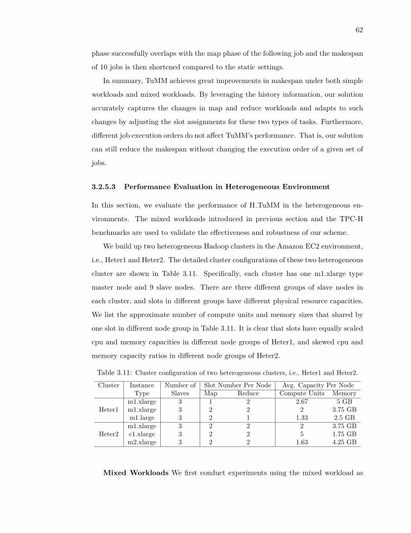
62

phase successfully overlaps with the map phase of the following job and the makespan

of 10 jobs is then shortened compared to the static settings.

In summary, TuMM achieves great improvements in makespan under both simple

workloads and mixed workloads. By leveraging the history information, our solution

accurately captures the changes in map and reduce workloads and adapts to such

changes by adjusting the slot assignments for these two types of tasks. Furthermore,

different job execution orders do not affect TuMM’s performance. That is, our solution

can still reduce the makespan without changing the execution order of a given set of

jobs.

3.2.5.3 Performance Evaluation in Heterogeneous Environment

In this section, we evaluate the performance of H TuMM in the heterogeneous en-

vironments. The mixed workloads introduced in previous section and the TPC-H

benchmarks are used to validate the effectiveness and robustness of our scheme.

We build up two heterogeneous Hadoop clusters in the Amazon EC2 environment,

i.e., Heter1 and Heter2. The detailed cluster configurations of these two heterogeneous

cluster are shown in Table 3.11. Specifically, each cluster has one m1.xlarge type

master node and 9 slave nodes. There are three different groups of slave nodes in

each cluster, and slots in different groups have different physical resource capacities.

We list the approximate number of compute units and memory sizes that shared by

one slot in different node group in Table 3.11. It is clear that slots have equally scaled

cpu and memory capacities in different node groups of Heter1, and skewed cpu and

memory capacity ratios in different node groups of Heter2.

Table 3.11: Cluster configuration of two heterogeneous clusters, i.e., Heter1 and Heter2.

Cluster Instance Number of Slot Number Per Node Avg. Capacity Per NodeType Slaves Map Reduce Compute Units Memory

m1.xlarge 3 1 2 2.67 5 GBHeter1 m1.xlarge 3 2 2 2 3.75 GB

m1.large 3 2 1 1.33 2.5 GBm1.xlarge 3 2 2 2 3.75 GB

Heter2 c1.xlarge 3 2 2 5 1.75 GBm2.xlarge 3 2 2 1.63 4.25 GB

Mixed Workloads We first conduct experiments using the mixed workload as

63

0 200 400 600 800 1000 1200 1400

Slo

t

Time (Sec)

0 200 400 600 800 1000 1200

Slo

t

Time (Sec)

(a) FIFO

0 200 400 600 800 1000 1200 1400

Slo

t

Time (Sec)

0 200 400 600 800 1000 1200

Slo

t

Time (Sec)

(b) H TuMM

Figure 3.21: Task execution times of a batch of mixed benchmarks under (a) FIFO and(b) H TuMM. The plots in the left (resp. right) column show the results from Heter1 (resp.Heter2) cluster. There are in total 30 (resp. 36) slots across Heter1 (resp. Heter2) cluster,i.e., there are at most 30 (resp. 36) running tasks in Heter1 (resp. Heter2) cluster at anygiven time.

Table 3.12: Maximum and minimum task execution times of each job across Heter1 cluster.

Map Tasks Reduce TasksBenchmarks Minimum (sec) Maximum (sec) Minimum (sec) Maximum (sec)Classification 6.5 24.1 9.5 15.9

Histogram Rating 8.5 24.8 9.7 25.5Inverted Index 5.1 17.4 16.5 48.1Word Count 11.5 31.4 12.6 25.2

Grep 6.7 25.1 12.7 29.5

described in Section 3.2.5.2, where the size of input data is 8GB and the data block

size is set to 64MB such that each job has 128 map tasks. Additionally, the number of

reduce tasks from each job is set to be 150 and 80 for the Inverted Index benchmark

and the remaining benchmarks, respectively.

In order to investigate the impact of heterogeneous environments on Hadoop per-

formance, we measured the maximum and minimum task execution times for each

job across different slave nodes in Heter1 cluster. As shown in Table 3.12, each job’s

task execution times are no longer uniform, for example, the slowest map task(s) of

a Classification job could almost run four times longer than the fastest one(s). We

interpret this effect by observing the variance of resource capacity among the slots on

different slave nodes.

Figure 3.21 illustrates the task execution details (i.e., the running period of each

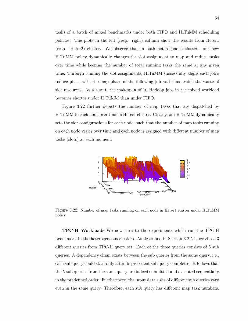
64

task) of a batch of mixed benchmarks under both FIFO and H TuMM scheduling

policies. The plots in the left (resp. right) column show the results from Heter1

(resp. Heter2) cluster. We observe that in both heterogenous clusters, our new

H TuMM policy dynamically changes the slot assignment to map and reduce tasks

over time while keeping the number of total running tasks the same at any given

time. Through tunning the slot assignments, H TuMM successfully aligns each job’s

reduce phase with the map phase of the following job and thus avoids the waste of

slot resources. As a result, the makespan of 10 Hadoop jobs in the mixed workload

becomes shorter under H TuMM than under FIFO.

Figure 3.22 further depicts the number of map tasks that are dispatched by

H TuMM to each node over time in Heter1 cluster. Clearly, our H TuMM dynamically

sets the slot configurations for each node, such that the number of map tasks running

on each node varies over time and each node is assigned with different number of map

tasks (slots) at each moment.

1 2 3 4 5 6 7 8 9 0 200 400 600 800 1000 1200 1400

0

1

2

3

nodes

time(sec)

0 0.5 1 1.5 2 2.5 3

Figure 3.22: Number of map tasks running on each node in Heter1 cluster under H TuMMpolicy.

TPC-H Workloads We now turn to the experiments which run the TPC-H

benchmark in the heterogeneous clusters. As described in Section 3.2.5.1, we chose 3

different queries from TPC-H query set. Each of the three queries consists of 5 sub

queries. A dependency chain exists between the sub queries from the same query, i.e.,

each sub query could start only after its precedent sub query completes. It follows that

the 5 sub queries from the same query are indeed submitted and executed sequentially

in the predefined order. Furthermore, the input data sizes of different sub queries vary

even in the same query. Therefore, each sub query has different map task numbers.

65

For example, in this set of experiments, the first sub query of all the three queries has

the largest input data size and thus most map tasks are clustered in the first few sub

queries, while the following sub queries have relatively small amount of map tasks.

We submit the 3 queries (i.e., TPCH-Q15, TPCH-Q16 and TPCH-Q18) to the

cluster at the same time, such that the sub queries of each query could interleave

with each other. The makespans of these three TPC-H queries in two heterogeneous

clusters (i.e., Heter1 and Heter2) are shown in Table 3.13 and the execution details

of these queries are further plotted in Figure 3.23. We observe that by dynamically

adjusting slot assignments on each node, H TuMM improves the performance (i.e.,

reducing the makespan) of all the three TPC-H queries when compared to FIFO.

Such performance improvement can be consistently observed in both heteregeneous

clusters. Figure 3.23 further illustrates that the map and reduce phases are well

aligned under the H TuMM policy.

Table 3.13: Makespans of TPC-H queries under FIFO and H TuMM in two heterogeneousclusters. The numbers in the parentheses are the relative improvements against FIFO.

Cluster Query FIFO H TuMMQ15 523.6 465.0 (11.1%)

Heter1 Q16 564.1 495.3 (12.2%)Q18 598.4 529.2 (11.5%)Q15 452.0 397.7 (12.0%)

Heter2 Q16 491.9 437.1 (11.1%)Q18 519.7 456.4 (12.4%)

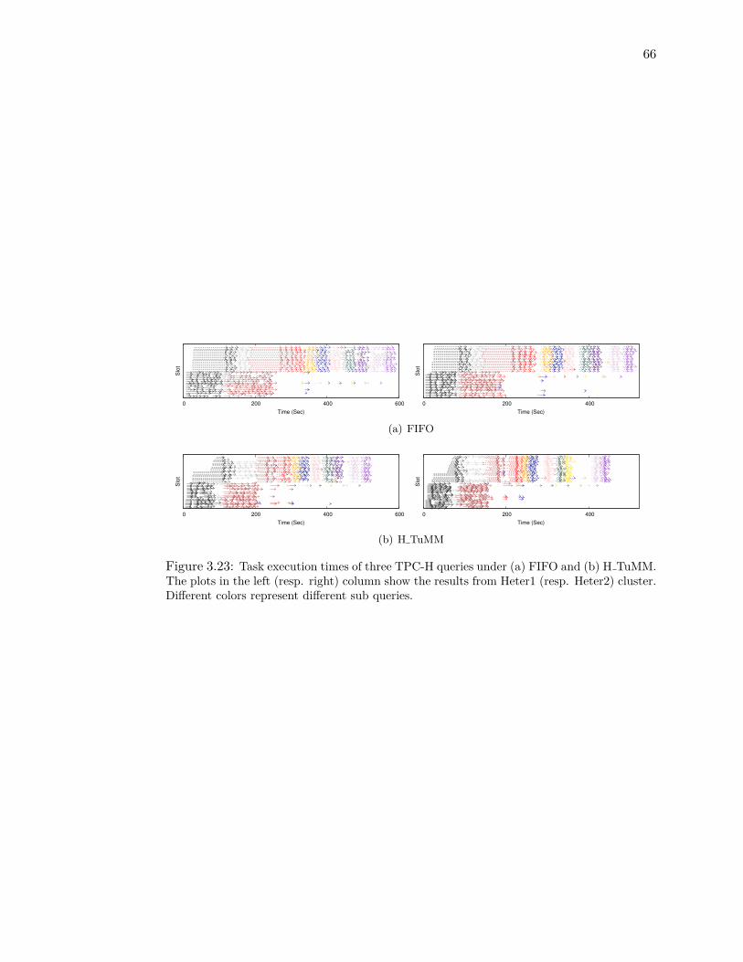
66

0 200 400 600

Slo

t

Time (Sec)

0 200 400

Slo

tTime (Sec)

(a) FIFO

0 200 400 600

Slo

t

Time (Sec)

0 200 400

Slo

t

Time (Sec)

(b) H TuMM

Figure 3.23: Task execution times of three TPC-H queries under (a) FIFO and (b) H TuMM.The plots in the left (resp. right) column show the results from Heter1 (resp. Heter2) cluster.Different colors represent different sub queries.

67

3.3 Related Work

Scheduling in Hadoop system has already received lots of attention. An early well

known work of Matei Zaharia et al. [37] proposed Fair scheduler which has been widely

adopted by Hadoop users since it is suitable for shared clusters. However, its objective

is not to optimize the system performance.

Scheduling performance is of great importance in Hadoop system and draws lots

of research attention. In [38], a delay scheduler was proposed to improve performance

of Fair scheduler by increasing data locality. It simply delays a task assignment for

a while when there is no local data available. This improvement is at task level, and

can be combined with our proposed works. Quincy scheduler [39] considered similar

direction and found a fair assignment while considering locality by formulating and

solving a minimum flow network problem. However, it is limited due to its high

computation complexity. In [40], Sandholm et. al. considered the profit of the service

provider and proposed a scheduler that splits slots to users according to the bids they

pay instead of fair share. The efficiency of scheduler is not considered in their work.

Joel Wolf et. al. proposed a slot allocation scheduler called FLEX [41] that could

optimize towards a given scheduling metric, e.g., average response time, makespan,

etc., by sorting jobs with generic schemes before allocating slots. Verma et al. [42]

introduced a heuristic to minimize the makespan of a set of independent MapReduce

jobs by applying the classic Johnson’s algorithm.

Job size based scheduling are also well studied in Hadoop system in recent years.

Mario Pastorelli et. al. [43] proposed HFSP, which closely assembles the Shortest

Remaining Processing Time (SRPT) algorithm with aging in Hadoop system to im-

prove efficiency. Deadline or SLA aware scheduling is also well studied in Hadoop

context. An early work of Kc and Anyanwu [44] address the problem of scheduling

jobs to meet user-provided deadlines, but assume job runtime to be an input to the

scheduler. Another deadline based scheduler was proposed in [45], which utilizes the

earliest deadline first (EDF) policy to sort jobs and adopts the Lagrange optimization

method to find out the minimum map and reduce slots number requirements of jobs

to meet their deadline. This solution requires a detailed profile for each job to pro-

vide its execution times of map and reduce tasks. Jorda Polo et al. [29] estimated the

68

task execution time of a MapReduce job from the average execution time of already

finished tasks of that job, and calculated the slots number a job needs based on its

deadline and estimated task execution time. We partly adopt the method to help

estimate the job size of each user in our proposed LsPS scheduler. Different deadline

and locality aware scheduling algorithms were evaluated with empirical analysis for

Hadoop system in [46].

Some other works focus on theoretical understanding of scheduling problem in

Hadoop system and give approximate scheduling algorithms [26,47]. Chang et al. [47]

proposed a 2-approximate scheduling algorithm. However, their assumption that there

are no precedence relationships between different tasks belonging to a given job is not

true in real-world Hadoop system. Benjamin et al. [26] formalized job scheduling

problem in MapReduce system as a generalization of the two-stage flexible flow-shop

problem and gave the off-line and on-line version of approximate algorithm. Their

work assumes that the execution time of tasks are known.

Furthermore, the heterogeneousness of system and jobs’ resource requirements are

considered in many research works to improve the scheduling. M. Zaharia et al. [48]

indicated that the Hadoop speculative execution will lead to poor performance in

heterogeneous Hadoop environments. They thus proposed LATE scheduler which

stops unnecessary speculative executions. [49] also focused on improving speculative

task execution by efficiently determine which tasks should be picked for duplicate

execution. [21] considered the difference of resources requirements of Hadoop jobs and

proposed a dominant resource fairness policy to fairly assign resources instead of slots.

This policy is implemented in the next generation Hadoop (YARN) system. Tian et

al. [50] propose a mechanism to concurrently schedule where IO-bound and CPU-

bound jobs, to avoid conflicts on single type of resource. The design of SkewTune [51]

greatly mitigates the issue of data skewness in Hadoop system with a plug-in module

to improve the job running efficiency. In [52], the authors proposed Tarazu, which

adaptively allows task stealing from slow nodes, as well as re-balancing loads of reduce

tasks running on slow and fast nodes.

69

3.4 Summary

In enterprise Hadoop MapReduce platforms, it is common practice to share the core

MapReduce cluster among multiple tenants with different kind of applications. In

general, these applications can be characterized into ad-hoc on-line queries and off-

line batch jobs, and have different prime performance concerns. For the ad-hoc query

jobs, the average response time is important for user experience while makespan is

more important for off-line jobs. In the proposed work, we first design an adaptive

scheduling technique that captures the present job size patterns of users and leverages

this knowledge to improve the system performance in terms of average job response

time. Performance of the proposed scheduler is evaluated in both simulators and

Amazon EC2 clusters under diverse workloads. We further propose a slot resource

management scheme to enable dynamic slot configuration in Hadoop MapReduce clus-

ter. The main objective is to improve resource utilization and reduce the makespan

of a batch of jobs. To meet this goal, the presented scheme introduces two main com-

ponents: Workload Monitor periodically tracks the execution information of recently

completed tasks and estimates the present workloads of map and reduce tasks; Slot

Assigner dynamically allocates the slots to map and reduce tasks by leveraging the

estimated workload information. The scheme is implemented upon Hadoop v0.20 and

evaluated with representative MapReduce benchmarks and TPC-H query sets in both

homogeneous and heterogeneous EC2 clusters.

70

Chapter 4

Resource Management for

Hadoop YARN

With the rapid growth of the demand on large-scale data processing and analysis, the

original Hadoop MapReduce system has met several bottlenecks. First, the centralize

JobTracker becomes performance bottleneck when cluster expands to thousands of

machines. Secondly, the coarse-grained resource management based on slot concept

is not suitable for higher resource utilization requirements. Moreover, the MapRe-

duce framework, although serves as a general purpose data processing scheme, is

not efficient for streaming data processing and iterative data processing. Therefore,

Hadoop has recently evolved into its second generation, Hadoop YARN - yet another

resource negotiator. As discussed in Section 2.3, Hadoop YARN separates the two

major functionalities of the JobTracker, i.e., resource management and job schedul-

ing / job monitoring and coordination, in the first generation Hadoop. A global

ResourceManager(RM) is in charge of cluster resource management and job schedul-

ing, and a per-application ApplicationMaster(AM) is required for negotiate resources

for tasks in application and monitor task executions. By splitting the job coordina-

tion from RM, YARN system is more horizontally scalable than the first generation

Hadoop. Furthermore, since RM becomes a pure scheduler, YARN system supports

different frameworks other than MapReduce, such that users can co-deploy multiple

frameworks on the same cluster and choose the most suitable framework for different

applications. However, the fine-grained resource allocation in YARN system and the

71

co-deployment of different frameworks introduce new challenges to efficient resource

management. In this section, we focus on developing new scheduler that improves ef-

ficiency of MapReduce jobs in YARN platform and new resource management scheme

that improves resource utilization and task throughput of YARN cluster.

72

4.1 Scheduling for YARN MapReduce

Hadoop YARN system abandons the coarse-grained “slot” configuration and evolves

into the fine-grained resource management. The widely adopted scheduling policies

in Hadoop system, e.g., FIFO, Fair, Capacity, however, still keep the same logic as

in the first generation Hadoop system. As described in Section 2.4, the FIFO policy

still sorts waiting jobs according to their submission time for scheduling, the Fair and

Capacity scheduler assign shares of cluster resources, in terms of memory instead of

slots, to jobs in different queues. Dominant Resource Fairness (DRF) scheduler is

a variant of Fair that introduced to handle multi-resource allocation, e.g., cpu and

memory, in YARN by assigning all jobs to get on average an equal share on their

dominant resource requirements. We find that these commonly adopted schedulers

are still not performing well for scheduling a batch of MapReduce jobs efficiently

under the fine-grained resource sharing platform. For example, while it is obviously

more efficient to run cpu intensive jobs and memory intensive jobs simultaneously, the

FIFO scheduler forces jobs to run sequentially which leads to unnecessary resource

idleness. Moreover, current resource sharing based schedulers omit considering the

dependency between MapReduce tasks which actually has a critical impact on the

efficiency especially when there are multiple jobs running concurrently in cluster.

Therefore, in this work, we present a new Hadoop YARN scheduling algorithm,

named HaSTE [20], which aims at efficiently utilizing cluster resources for scheduling

map/reduce tasks in Hadoop YARN and improving the makespan of MapReduce jobs.

HaSTE meets these goals by leveraging the requested resources, resource capacities,

and the dependency between tasks. Specifically, our solution dynamically schedules

tasks for execution when resources become available based on each task’s fitness and

urgency. Fitness essentially refers to the gap between the resource demand of tasks

and the residual resource capacity of nodes. This metric has been commonly con-

sidered in other resource allocation problems in the literatures. The second metric,

urgency, is designed to quantify the “importance” of a task in the entire process. It al-

lows us to prioritize all the tasks from different jobs and more importantly, catches the

dependency between tasks. An aggregation function is used to combines the fitness

and urgency to compare all candidate tasks for efficient schedule.

73

4.1.1 Problem Formulation

We consider that a set of n jobs {J1, J2, . . . , Jn} are submitted to a Hadoop YARN

cluster consisting of m servers, {S1, S2, . . . , Sm}. Each job consists of map tasks and

reduce tasks. We consider all the tasks in n jobs as a set T and assign each task

a unique index number, i.e., ti represents the i-th task in the system. Each job Ji

is then represented by a set of tasks. We further define two subsets MT and RT to

represent all the map tasks and reduce tasks, respectively, i.e., T = MT∪RT . MT∩Ji

(RT ∩ Ji) represents all the map (reduce) tasks of job Ji. In addition, assume that k

types of computing resources are considered in the system, indicated by r1, r2, . . . , rk.

Note that in the current YARN system, only two resources are included, memory

and cpu. Here we use k to define the problem with a general setting so that potential

extensions can involve other types of resources, e.g., network bandwidth and disk I/O.

In the rest of the paper, r1 and r2 represent memory and cpu resources, respectively.

We use a two-dimensional matrix C to represent the resource capacity in the cluster.

C[i, j] indicates the amount of available resource rj at server Si, where i ∈ [1,m] and

j ∈ [1, k]. This matrix C is available to the scheduler after the cluster is launched

and the values in C are updated during the execution of jobs upon each heartbeat

message received from NodeManagers.

In YARN, each task can request for user-specified resources. All map/reduce tasks

in a job share the same resource requirement. For a task ti ∈ T , R[i, j] is defined

to record the amount of resource rj requested by ti, where R[p, j] = R[q, j] if tp and

tq are the same type of tasks (either both map tasks or both reduce tasks) from the

same job. The Hadoop scheduler can assign a task ti to a work node Sj for execution

as long as ∀p ∈ [1, k],R[i, p] ≤ C[j, p]. In this paper, given C and R, our goal is to

design an efficient scheduler that can help the cluster finish all the MapReduce jobs

with the minimum time (i.e., minimize the makespan). More specifically, let sti be

the starting time of task ti ∈ T , τi be the execution time of ti, and xij indicate the

association between ti and Sj , i.e., xij is 1 if task ti is assigned to worker node Sj .

74

Then our scheduling problem is to derive sti and xij in order to

minimize: max{sti + τi}, ∀i ∈ T

s.t.∑

j∈[1,m]xij = 1,∀ti ∈ T ; (4.1)

∑ti∈A(θ)

xijR[i, p] ≤ C[j, p], j ∈ [1,m], p ∈ [1, k], θ > 0; (4.2)

xij ∈ {0, 1}, sti ≥ 0, ∀i, j.

Here time is measured as a discrete value which is multiple of the time unit. θ

represents a particular time point, and A(θ) is defined as the set of active tasks at

time θ, A(θ) = {ti ∈ T |sti ≤ θ ≤ sti + τi}. Therefore, constraint (4.1) specifies

that each task could be assigned to exactly one NodeManager, and constraint (4.2)

requires that the resources consumed by all active tasks at a particular worker node

Sj cannot exceed its resource capacity.

Assume τi is available and each map/reduce task is independent, our scheduling

problem is equivalent to general resource constrained scheduling problem which has

been proved to be NP-complete [53]. Many heuristics have been proposed for solving

the problem. Most of them, however, are not practical to be directly implemented in

the Hadoop YARN system. The main issue is that the processing time τi of each task

ti is required to determine the schedule in the conventional solutions. In practice, the

value of τi cannot be known as a prior before its execution in the system. Profiling

or other run time estimation techniques may be applied to roughly estimate the

execution time of map tasks [29,45]. However, it is extremely hard, if not impossible,

to predict the execution times of reduce tasks in a cluster where multiple jobs could

be running concurrently. In Hadoop YARN, the reduce tasks of a MapReduce job

consist of two main stages, shuffle and reduce. In the shuffle stage, the output of

each map task of the job is transferred to the worker nodes which host the reduce

tasks, while computation in the reduce stage starts when all the input data are ready.

Therefore, the execution time of a reduce task are dependent on several map-related

factors, such as the execution times of all map tasks and the size of the intermediate

output data. In this paper, we aim to develop a more practical heuristic that does

not require any prior knowledge of task execution times.

75

4.1.2 Sketch of HaSTE Design

We design a scheduler that consists of two components, initial task assignment and

real-time task assignment. First, initial task assignment is executed when the cluster

is just started and all ApplicationMasters have submitted the resource requests for

their MapReduce tasks to the scheduler. The goal of initial task assignment is to

assign the first batch of tasks for execution while the rest of tasks remain pending

in the system queue. Specifically, initial task assignment algorithm needs to select a

subset of pending tasks and select a hosting work node for each of them for execution.

On the other hand, real-time task assignment is launched during the execution of all

the jobs when tasks are finished and the corresponding resources are released. When

new resources become available at a worker node, the NodeManager will notify the

scheduler through heartbeat messages. Then the scheduler will execute real-time task

assignment to select one or more tasks from the pending queue and assign them to

the worker node with new resources available. Compared to initial task assignment,

real-time task assignment is triggered by heartbeat messages with resource capacity

update and only dispatches tasks to the hosting work node, i.e., the sender of the

heartbeat message.

In our design, without prior knowledge of the execution time, we exploit the greedy

strategy to develop both initial task assignment and real-time task assignment algo-

rithms. Initial task assignment is formulated as a variant of the knapsack problem.

We then use dynamic programming to derive the best task assignment in the begin-

ning. Real-time task assignment is a more complex problem involving the progress

of all active tasks and the dependency between tasks. We develop an algorithm that

considers fitness and urgency of tasks for determining the appropriate task to execute

on-the-fly.

4.1.3 Initial Task Assignment

The objective of this component is to select a set of tasks to start. Since the execution

of each task is unknown, it is impossible to yield the optimal solution at this point.

Therefore, we adopt the greedy strategy and simplify our objective to be maximiz-

ing the resource utilization after initial task assignment. If there is only one type

76

of resource, then this problem is equivalent to the typical knapsack problem. Con-

sider each worker node as a knapsack, the resource capacity refers to the knapsack

capacity. Correspondingly, each task can be considered as an item and the requested

resource amount is both the weight and the value of the item. The optimal solu-

tion to the converted knapsack problem will yield the maximized resource utilization

in our problem setting. However, the Hadoop YARN system defines two resources

(recall that we consider a general setting of k resources) in which case our problem

cannot directly reduce to the knapsack problem. We thus need a quantitative means

to compare different types of resources, e.g., Is utilizing 100% cpu and 90% memory

better than utilizing 90% cpu and 100% memory? We then assume that the cluster

specifies a weight wi for each resource ri. The initial task assignment problem can be

formulated as follows:

maximize:∑ti∈T

(∑

j∈[1,m]xij ·

∑p∈[1,k]

wp · R[i, p])

s.t.∑

j∈[1,m]xij ≤ 1,∀ti ∈ T ;

∑ti∈T

xij · R[i, p] ≤ C[j, p],∀j ∈ [1,m], p ∈ [1, k].

We design an algorithm using dynamic programming to solve the problem. The

details are illustrated in the following Algorithm 4.1. The main algorithm is simply

a loop that assigns tasks to each of the m servers (lines 1–2). The core algorithm is

implemented in the procedure AssignTask(j, T ), i.e., select tasks from T to assign

to server Sj . We design a dynamic programming algorithm with two 2-dimensional

matricesM and L, whereM[a, b] is the maximum value of our objective function with

a capacity <a,b> and L records the list of tasks that yield this optimal solution. The

main loops fill all the elements in M and L (lines 4–17). Eventually, the algorithm

finds the optimal solution (line 18) and assigns the list of tasks to Sj (lines 19–23).

When filling an element in the matrices (lines 6–17), we enumerate all candidate tasks

and based on the previously filled elements, we check: (1) if the resource capacity is

sufficient to serve the task (lines 9-12); and (2) if the resulting value of the objective

function is better than the current optimal value (lines 13-16). If both conditions are

satisfied, we update the matrices M and L (line 16-17).

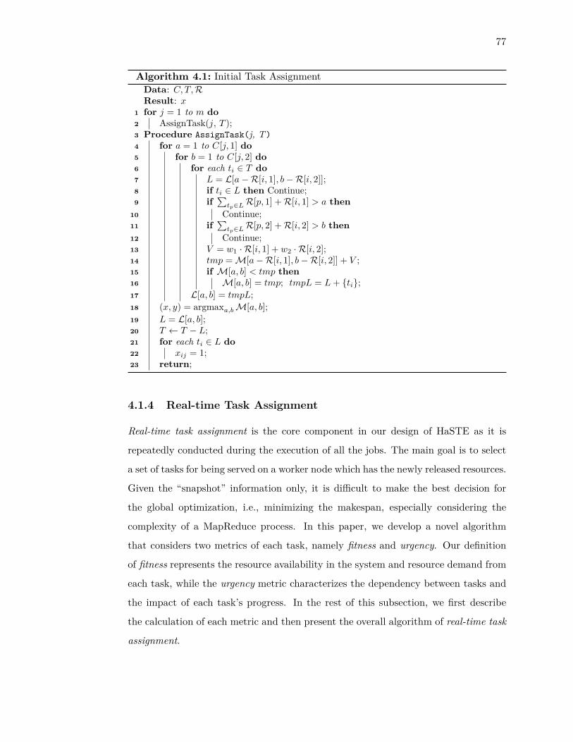
77

Algorithm 4.1: Initial Task AssignmentData: C, T,RResult: x

1 for j = 1 to m do2 AssignTask(j, T );3 Procedure AssignTask(j, T)4 for a = 1 to C[j, 1] do5 for b = 1 to C[j, 2] do6 for each ti ∈ T do7 L = L[a−R[i, 1], b−R[i, 2]];8 if ti ∈ L then Continue;9 if

∑tp∈LR[p, 1] +R[i, 1] > a then

10 Continue;11 if

∑tp∈LR[p, 2] +R[i, 2] > b then

12 Continue;13 V = w1 · R[i, 1] + w2 · R[i, 2];14 tmp =M[a−R[i, 1], b−R[i, 2]] + V ;15 if M[a, b] < tmp then16 M[a, b] = tmp; tmpL = L+ {ti};17 L[a, b] = tmpL;18 (x, y) = argmaxa,bM[a, b];19 L = L[a, b];20 T ← T − L;21 for each ti ∈ L do22 xij = 1;23 return;

4.1.4 Real-time Task Assignment

Real-time task assignment is the core component in our design of HaSTE as it is

repeatedly conducted during the execution of all the jobs. The main goal is to select

a set of tasks for being served on a worker node which has the newly released resources.

Given the “snapshot” information only, it is difficult to make the best decision for

the global optimization, i.e., minimizing the makespan, especially considering the

complexity of a MapReduce process. In this paper, we develop a novel algorithm

that considers two metrics of each task, namely fitness and urgency. Our definition

of fitness represents the resource availability in the system and resource demand from

each task, while the urgency metric characterizes the dependency between tasks and

the impact of each task’s progress. In the rest of this subsection, we first describe

the calculation of each metric and then present the overall algorithm of real-time task

assignment.

78

4.1.4.1 Fitness

Using fitness in our design is motivated by the greedy solution to the classic bin

packing problem. We first note that some special cases of our problem are equivalent

to the classic bin packing problem. Assume that all submitted jobs have only one

type of tasks and all tasks are independent to each other. Also, assume that the

execution times of all tasks are the same, say u time units. Our scheduling problem

thus becomes packing tasks into the system for each time unit. The total resource

capacity is considered as the bin size and the makespan is actually the number of bins.

Thus, finding the optimal job scheduling in this setting is equivalent to minimizing

the number of bins in the bin packing problem. The classic bin packing considers

only one type of resource and has been proven to be NP-hard. A greedy heuristic,

named First Fit Decreasing (FFD), is widely adopted to solve the problem because it

is effective in practice and yields a 119 OPT +1 worst case performance [54]. The main

idea of FFD is to sort tasks in a descending order of the resource requirements and

keep allocating the first fitted tasks in the sorted list to the bins. Figure 4.1 illustrates

how FFD can improve the makespan and resource utilization when scheduling two

jobs with different memory requirements.

1G

3G

t0 t1 t2 t3 t4 t5

Memory Capacity: 4G

(a) FIFO

1G

3G

t0 t1 t2 t3 t4 t5

Memory Capacity: 4G

(b) FAIR

1G

3G

t0 t1 t2 t3 t4 t5

Memory Capacity: 4G

(c) FFD

Figure 4.1: Scheduling two jobs under (a) FIFO, (b) Fair and (c) FFD, where a worker nodewith 4G memory capacity is processing two jobs each with 4 tasks. Job 1 arrives first and eachof its task requests 1G memory (blue blocks), while each task of Job 2 requests 3G memory,see yellow blocks. Assume that the execution time of each task is one time unit. Thus, theFFD scheduler uses 4 time units to finish both jobs while FIFO and Fair need 5 time units.

In fact, with two types of resources (memory and cpu) supported in Hadoop

YARN, the simplified scheduling problem is equivalent to the vector bin packing

problem in the literature. Different variants of FFD have been studied for solving the

vector bin packing problem [55]. The FFD-DotProduct (dubbed as FFD-DP) method

has been shown to be superior under various evaluation sets. Therefore, we adopt the

79

FFD-DP method to schedule map and reduce tasks with two resource requirements.

Specifically, we define fitness as:

Fij =∑

p∈[1,k]R[i, p] · C[j, p] · wp. (4.3)

Real-time task assignment uses Eq.(4.3) to calculate a fitness score for each pending

task ti when selecting tasks to be executed on the worker node Sj . Recall that for each

resource rp, R[i, p] is the requested amount from ti, C[j, p] is the resource capacity at

Sj , and wp is the weight of the resource. Intuitively, we prefer to select the task with

the highest fitness score. Therefore, real-time task assignment can sort all the pending

tasks in the descending order of their fitness scores, and then assign the first task to

the worker node Sj . After updating Sj ’s resource capacity, real-time task assignment

will repeat this selection process to assign more tasks until there is no sufficient

resource on Sj to serve any pending tasks. The FFD-DP algorithm works well with

multiple resource types since it is aware of the skewness of resource requirements. For

example, assume that there two types of tasks with different resource requirements:

one requests <1 GB, 3 cores> and the other requests <3 GB, 1 core>; and real-time

task assignment tries to assign tasks to a worker node with residual capacity of <10

GB, 6 cores>. The FFD-DP algorithm will choose 3 tasks of type II and 1 task of type

I, which results in 100% resource utilization. The following table shows the fitness

scores of these two types of tasks at each iteration of the algorithm.

Capacity <10,6> <7,5> <4,4> <3,1>Type I <1 GB, 3 cores> 28 22 16 6Type II <3 GB, 1 core> 36 26 16 10

4.1.4.2 Urgency

Scheduling in Hadoop YARN is more complex than the regular job scheduling problem

due to the dependency between map and reduce tasks. Considering fitness alone may

not always lead to good performance in practice. Although there has been previous

work [56–59] on job scheduling under the dependency constraints, their solutions

cannot be directly applied to our problem because the dependency between map

and reduce tasks is quite different from the dependency defined in these works. In

traditional scheduling problems, a task tj is said to be dependent on task ti, i.e.,

80

ti ≺ tj , if tj cannot start before ti has been completed. However, in the MapReduce

framework, reduce tasks, although depend on the outputs of all map tasks, can start

before the completion of all map tasks for retrieving the intermediate data from the

completed map tasks. This early start is configured by a system parameter “slowstart”

and renders a better performance in practice.

Consequently, the execution of the reduce tasks are highly dependent on the ex-

ecution of map tasks,. Indeed, such dependency relationship has been known by

ApplicationMasters when making reduce task requirements. A new metric, named

“Ideal Reduce Memory Limit”, is calculated as the product of the progress of map

tasks and the total “available” memory for the corresponding job. The resource limit

of reduce tasks increases gradually with the progress of map tasks. An Application-

Master sends new reduce task requests to the ResourceManager only when the present

resource limit is enough for running more reduce tasks.

However, we observed that the current schedulers in Hadoop YARN, which are

designed for more general task scheduling, fail to recognize the impact of dependency

in MapReduce jobs and may lead to ineffective resource assignments and poor perfor-

mance as well. For example, a job that has already launched many reduce tasks may

not be able to have all its map tasks to be executed right away due to resource con-

tention among other jobs; the launched reduce tasks will keep occupying the resources

when waiting for the completion of all maps tasks of the same job. This incurs low

utilization of resources that are allocated to those reduce tasks.

To address the above issue, HaSTE uses a new metric, named “urgency”, to cap-

ture the performance impact caused by the dependency between map and reduce

tasks of MapReduce jobs. Specifically, we have the following main scheduling rules

associated with the urgency.

R1. A job with more progress in its map phase, will be more urgent to schedule its

map tasks. This rule can boost the completion of the entire map phase and further

reduce the execution time of the launched reduce tasks.

R2. A job with more resources allocated to its running reduce tasks will be more

urgent to schedule its map tasks in order to avoid low resource utilization when its

reduce tasks are waiting for the completion of map tasks.

R3. Reduce tasks should be more urgent than map tasks of the same job if the ratio

81

between resources occupied by currently running reduces and all currently running

tasks is lower than the progress of map phase, vice versa.

In summary, R1 and R2 are used to compare the urgency between two different

jobs while the urgency of map/reduce tasks from the same job is compared by R3.

We have the following equations to calculate the urgency score Umi (U ri ) for each map

(reduce) task from job i:

Umi = AmiTmi· (Ari ·Rri +Aami ·Rami ), (4.4)

U ri = Umi ·AmiTmi· O

mi ·Rmi +Ori ·Rri

Ori ·Rri. (4.5)

Here Ami /Ari /A

ami represents the number of map/reduce/ApplicationMaster tasks

that have been assigned for job i, and Rmi /Rri /R

ami represents the resource require-

ment of a single map/reduce/ApplicationMaster task, i.e., the weighted summation of

memory and cpu requirements. Tmi represents the total number of map tasks of job i.

Omi /Ori represents the number of running map/reduce tasks of job i that are currently

occupying system resources. All these metrics are accessible to the scheduler in the

current YARN system. Therefore, we implemented our new scheduler as a pluggable

component to YARN without any needs of changing other components.

4.1.4.3 On-line Scheduler

Now, we turn to summarize the design of HaSTE by integrating the two new metrics,

i.e., fitness and urgency, into the scheduling decision.

Once a node update message is received from a NodeManager, the scheduler first

creates a list of all resource requests that can fit the remaining resource capacity

of that node. Meanwhile, the scheduler calculates the fitness and urgency scores of

those chosen resource requests, and obtains the preference score for each request by

summing up the normalized fitness and urgency scores, see Eq.(4.6).

Pi = Fi − FminFmax − Fmin

+ Ui − UminUmax − Umin

, (4.6)

where Fmax and Fmin (resp. Umax and Umin) record the maximum and minimum

fitness (resp. urgency) scores among these requests.

Such preference scores are then used to sort all resource requests in the list. The

resource request with the highest score will be chosen for being served. Note that

82

each resource request can actually represent a set of task requests since tasks with

the same type and from the same job usually have the same resource requirements.

The scheduler will then choose a task that has the best locality (i.e., node local or rack

local) and assign that task to the NodeManager. One special type of task request is

the request for ApplicationMaster. Such requests always have the highest preference

score in HaSTE due to its special functionality, i.e. submitting resource requirements

and coordinating the execution of a job’s tasks.

Finally, we remark that the complexity of our scheduling algorithm is O(n logn)

which is determined by the sorting process. Here n is the number of running jobs

rather than the number of running tasks, since all tasks with the same type and from

the same job could be represented in a single resource request and then have the same

preference score. Therefore, HaSTE is a light-weighted and practical scheduler for the

Hadoop YARN system.

4.1.5 Evaluation

In this section, we evaluate the performance of HaSTE by conducing experiments in a

Hadoop YARN cluster. We implemented both HaSTE and FFD-DotProduct (abbrev.

FFD-DP) schedulers in Hadoop YARN version 2.2.0 and compared HaSTE with three

built-in schedulers (i.e., FIFO, Fair and DRF) and FFD-DP. The performance metrics

considered in the evaluation include makespans of a batch of MapReduce jobs and

resource utilizations of the Hadoop YARN cluster.

4.1.5.1 Resource Requests of MapReduce Jobs

In our experiments, we consider different resource requirements such that a job can

be either memory intensive or cpu intensive. The resource requirements of map and

reduce tasks of a MapReduce job can be specified by the user when that job is sub-

mitted. The user should set the resource requirements equal to or slightly more than

the actual resource demands. Otherwise, a task will be killed if it uses more resources

than its resource demand1. Such a mechanism adopted in the YARN system can pre-1We note that the virtual cpu cores are not physically isolated for each task in the YARN system.

The number of virtual cpu cores requested for a task determines the priority of that task whencompeting for cpu times. Therefore, an inappropriate low request of virtual cpu cores is also notdesired because it may lead to insufficient cpu times that a task can get and dramatically delay the

83

vent malicious users from faking the resource requirements and thus from thrashing

the system. On the other hand, it is not proper either to request much more than

the actual demands because the concurrency level of MapReduce jobs and the actual

resource utilizations will be reduced and the performance will be degraded as well.

We note that how to set appropriate resource requirements for each job is discussed

in the next section. In our experiments, we vary the resource requirements for dif-

ferent jobs in order to evaluate the schedulers under various resource requirements,

but keep the resource requirements configuration the same under different scheduling

algorithms.

4.1.5.2 Experiment Results

Here, we conduct two sets of experiments in a Hadoop YARN cluster with 8 nodes,

each of which is configured with the capacity of 8GB memory and 8 virtual cpu cores,

i.e., <8G, 8cores> .

Simple Workload. In the first set of experiments, we consider a simple workload

which consists of four Wordcount jobs. Each job in this workload parses the same 3.5G

wiki category links input file. Therefore, all the four jobs have the same number of

map and reduce tasks. The map task number is determined by the input file size

and the HDFS block size which is set to 64MB in this experiment. As described

in Section 4.1.5.1, for different jobs, we vary the resource requirements on a single

type of resource for analyzing the impact of resource requirements on the scheduling

performance. The configurations of each job and their resource requirements are

shown in Table 4.1.

Table 4.1: Simple Workload Configuration.

Job ID #Map #Reduce Rm Rr

1 52 5 <1G, 2cores> <1G, 2cores>2 52 5 <1G, 3cores> <1G, 2cores>3 52 5 <1G, 4cores> <1G, 3cores>4 52 5 <1G, 5cores> <1G, 3cores>

Figure 4.2 shows the makespans and the average resource (mem and cpu) utiliza-

tions under different scheduling policies. Note that the resource utilization presented

in this work is the percentage of total cluster resources that have been assigned to

execution of that task.

84

0

200

400

600

800

1000

FIFO Fair DRF FFD-DP HaSTE 0

20

40

60

80

100

Tim

e(S

ec)

Per

cent

age(

%)

MakespanMemory-Usage

Cores-Usage

Figure 4.2: Makespans and average resource utilizations under the workload of 4 Wordcountjobs. The left y-axis shows the makespans (sec.) while the right y-axis shows the cpu andmemory resource utilizations (%).

MapReduce tasks, instead of actual run time resource usages of cluster nodes which

may be lower than the assigned resource amount. We observe that all the conventional

schedulers (i.e., FIFO, Fair, and DRF) cannot efficiently utilize the system resources,

e.g., under 60% cpu core utilization and under 30% memory utilization. Although

these conventional schedulers obtain similar resource utilizations, FIFO outperforms

Fair by 23.8% and DRF by 29.3%. That is because under Fair and DRF, when mul-

tiple jobs are running concurrently in the cluster, their reduce tasks are launched and

thus occupy many of the assigned resources, which may dramatically delay the exe-

cution of map phases. Therefore, running reduce tasks have to wait for map outputs

and cannot fully utilized their assigned resources. Similarly, the makespan under the

FFD-DP scheduling policy is 10% larger than under FIFO, although more system

resources are assigned for running tasks under FFD-DP, e.g., 86.6% cpu cores uti-

lization in average. HaSTE solves this problem by considering the impacts of both

resource requirements (i.e., fitness) and dependency between tasks (i.e., urgency) and

thus achieves the best makespan, which is, for example, 27% and 44.6% shorter than

FIFO and Fair, respectively.

Mixed Workload. To further validate the effectiveness of HaSTE, we conduct a

more complex workload which is mixed with both cpu and memory intensive MapRe-

duce jobs. Table 4.2 shows the detailed workload configuration, where the input data

for Terasort is generated through the Teragen benchmark, and the input for Word-

count and Wordmean is the wiki category links data. In this set of experiments, we

set the HDFS file block size to be equal to 128MB.

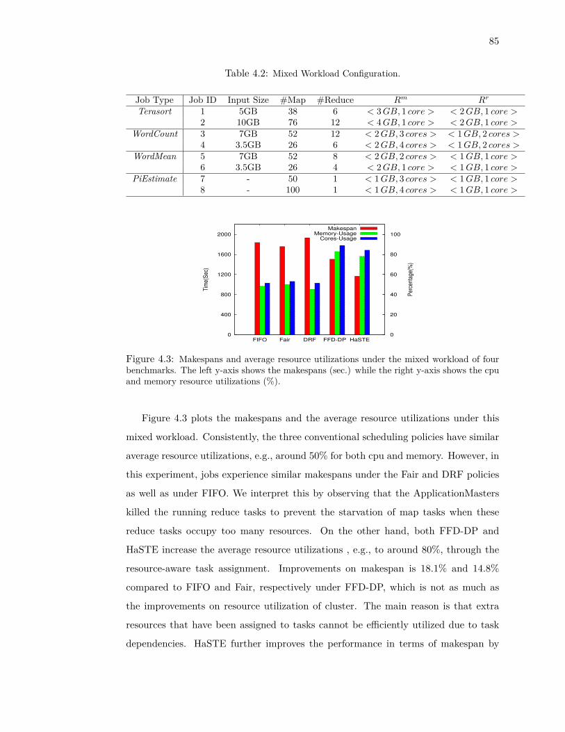
85

Table 4.2: Mixed Workload Configuration.

Job Type Job ID Input Size #Map #Reduce Rm Rr

Terasort 1 5GB 38 6 < 3GB, 1 core > < 2GB, 1 core >2 10GB 76 12 < 4GB, 1 core > < 2GB, 1 core >

WordCount 3 7GB 52 12 < 2GB, 3 cores > < 1GB, 2 cores >4 3.5GB 26 6 < 2GB, 4 cores > < 1GB, 2 cores >

WordMean 5 7GB 52 8 < 2GB, 2 cores > < 1GB, 1 core >6 3.5GB 26 4 < 2GB, 1 core > < 1GB, 1 core >

PiEstimate 7 - 50 1 < 1GB, 3 cores > < 1GB, 1 core >8 - 100 1 < 1GB, 4 cores > < 1GB, 1 core >

0

400

800

1200

1600

2000

FIFO Fair DRF FFD-DP HaSTE 0

20

40

60

80

100

Tim

e(S

ec)

Per

cent

age(

%)

MakespanMemory-Usage

Cores-Usage

Figure 4.3: Makespans and average resource utilizations under the mixed workload of fourbenchmarks. The left y-axis shows the makespans (sec.) while the right y-axis shows the cpuand memory resource utilizations (%).

Figure 4.3 plots the makespans and the average resource utilizations under this

mixed workload. Consistently, the three conventional scheduling policies have similar

average resource utilizations, e.g., around 50% for both cpu and memory. However, in

this experiment, jobs experience similar makespans under the Fair and DRF policies

as well as under FIFO. We interpret this by observing that the ApplicationMasters

killed the running reduce tasks to prevent the starvation of map tasks when these

reduce tasks occupy too many resources. On the other hand, both FFD-DP and

HaSTE increase the average resource utilizations , e.g., to around 80%, through the

resource-aware task assignment. Improvements on makespan is 18.1% and 14.8%

compared to FIFO and Fair, respectively under FFD-DP, which is not as much as

the improvements on resource utilization of cluster. The main reason is that extra

resources that have been assigned to tasks cannot be efficiently utilized due to task

dependencies. HaSTE further improves the performance in terms of makespan by

86

36.3% and 33.9% compared to FIFO and Fair, respectively.

0 5

10 15 20 25 30 35 40 45

0 500 1000 1500 2000

Mem

ory

Occupie

d

Time

(a) FIFO

job8job7job6job5job4job3job2job1

0 5

10 15 20 25 30 35 40 45

0 500 1000 1500 2000

Mem

ory

Occupie

d

Time

(b) Fair

job8job7job6job5job4job3job2job1

0 5

10 15 20 25 30 35 40 45

0 500 1000 1500 2000

Mem

ory

Occupie

d

Time

(c) DRF

job8job7job6job5job4job3job2job1

0

10

20

30

40

50

60

70

0 200 400 600 800 1000 1200 1400 1600

Mem

ory

Occupie

d

Time

(d) FFD-DP

job8job7job6job5job4job3job2job1

0

10

20

30

40

50

60

70

0 200 400 600 800 1000 1200

Mem

ory

Occupie

d

Time

(e) HaSTE

job8job7job6job5job4job3job2job1

Figure 4.4: Illustrating the memory resources that have been allocated to each job cross timeunder different scheduling policies.

To better understand how these scheduling policies work, we further plot the

runtime memory allocations in Figure 4.4. We observe that the precedence constraint

of FIFO policy and the fairness constraint of Fair and DRF policies can both lead to

inefficient resource allocation in the Hadoop YARN cluster. For example, when cpu

intensive jobs are running under the FIFO policy, see job 3,4,6,7 in Figure 4.4(a), the

87

scheduler cannot co-schedule memory intensive jobs at the same time, and a large

amount of memory resources in the cluster are idle for a long period. Under the

Fair and DRF policies, although all jobs share the resources, the fairness constraint,

i.e., all jobs should get equal shares on average, in fact hinders the efficient resource

utilizations. For example, when a node has < 1GB, 4 cores > available resources

and two tasks t1 and t2 with R1 =< 1GB, 4 cores > and R2 =< 1GB, 1 core > are

waiting for service, Fair may assign resources to t2 if this tasks now deserves more

share of resources, which will lead to a waste of 3 cpu cores on the node. We also

observe that by tuning the resource shares among different jobs, the FFD-DP policy

could achieve better resource utilizations across time. More importantly, HaSTE also

achieves high or even slightly higher resource utilizations across time. This is because

HaSTE allows jobs whose resource requirements can better fit the available resource

capacities to have higher chance to get resources and thus improves the resource

utilizations.

In summary, HaSTE achieves non-negligible improvements in terms of makespans

and resource utilizations when the MapReduce jobs have various resource require-

ments. By leveraging the information of job resource requirements and cluster re-

source capacities, HaSTE is able to efficiently schedule map/reduce tasks and thus

improve the system resource utilization. In addition, the makespans of MapReduce

jobs are further improved by taking the dependency between map and reduce tasks

into consideration when multiple jobs are competing for resources in the YARN clus-

ter.

88

4.2 Idleness Management of YARN System through

Opportunistic Scheduling

Popular resource management schemes, i.e., Hadoop YARN [7] and Mesos [8], both

adopt fine-grained resource management, i.e., leveraging the knowledge of task re-

source requirements, system residual resources, and scheduling policies to assign re-

sources to tasks of applications from different frameworks. Applications from different

frameworks need to send resource requests for their tasks, which consist of cpu and

memory demands, to a centralized resource manager. Scheduler resides in the resource

manager can then assign tasks based on global status, e.g., current resource assign-

ment to applications and residual resources on cluster nodes. High cluster resource

utilization level is expected under such resource management schemes based on the

following reasons. First, cluster resources are more effectively shared among multiple

applications and frameworks compared with static resource partitioning. Secondly,

resource assignments are performed at task level. Since tasks have relatively lower

resource demands and shorter life times than applications, it is easier to assign re-

sources for tasks and the assigned resources can also be recycled for future usage

quickly. Moreover, different resource types are considered when assigning resources

such that tasks can be efficiently co-assigned for better resource utilization, e.g., assign

cpu intensive tasks and memory intensive tasks to the same node.

However, these schemes still cannot fully utilize cluster resources. A production

cluster at Twitter managed by Mesos has reported to have aggregate cpu utilization

lower than 20% when reservations reach up to 80% [14], and Google’s Borg system

has reported aggregate cpu utilization of 25-35% while reserved cpu resources exceed

70% [15] . One main reason is that current resource management schemes always

reserve fixed amount of resources for each task according to its resource request. Yet,

we observe that tasks from many frameworks and applications actually have fluctuat-

ing resource usage patterns. As an example, reduce tasks in MapReduce framework

usually have low cpu utilization in their shuffle stage when they are waiting for map

tasks to generate outputs. And they become more cpu intensive after their shuffle

phases have finished, i.e., fetched all intermediate data from map tasks. Another

example is Spark tasks. When deployed on a YARN system, each spark task is an

89

executor that hosts multiple user-defined stages which may require different types

and amounts of resources. Even more, when Spark tasks serve interactive queries,

resource usage of these tasks can change frequently, e.g., being totally idle during

the user’s thinking time, and becoming busy and requesting more resources upon the

user’s query arrivals. Similarly, frameworks that process streaming data may keep a

large number of tasks being alive and waiting for streaming inputs for processing. Re-

source requirements thus have to change over time upon the arriving of incoming new

data which is unfortunately non-predictable. In these cases, fixing the assignment of

resources during a task’s lifetime becomes inefficient to fully utilize system resources.

Motivated by this problem, we present a new opportunistic scheduling approach

that helps resource management schemes to improve system resource utilization and

application throughput. The main idea of our approach is to leverage the knowledge

of actual run-time system resource utilizations for task assignment. That is, when

observing that a running task is idle or not fully utilizing its assigned resources, we

aggressively assign the spare resources for running eligible pending tasks. The key

issue to be addressed in our approach is how to reduce or avoid performance inter-

ference when running tasks are requiring more resources which have already been

assigned to others during their idle periods. To solve this problem, we restrict that

only tasks with short life times are eligible for stealing idle resources from running

tasks, i.e., opportunistic scheduling. Given that, we expect that (1) opportunistic

scheduled tasks have high chances to finish before running tasks requiring back their

resources, such that there are fewer severe resource contentions and performance in-

terferences, and (2) killing opportunistically assigned tasks upon resource contentions

will not result in significant work and resource waste. Different contention relief

policies are also designed for preventing performance interferences when detecting

resource contentions. We implement the new opportunistic scheduling approach in

Hadoop YARN, and evaluate its effectiveness with MapReduce and Spark workloads.

Experiment results show clear improvements on both cluster resource utilizations and

application response times.

90

4.2.1 Background and Motivation

4.2.1.1 Resource Capacity and Reservation in a Cluster

The current cluster resource management is based on resource reservation. Basically,

each cluster member declares its resource capacity, specifically the number of CPU

cores and the memory size. On the other hand, when submitting a job, the user needs

to specify the resource demand for each task of the job. A centralized resource man-

ager is responsible for allocating the resources to each pending task. Specifically, each

task will be executed in a resource container that occupies the amounts of resources

requested by the task. The resource manager may adopt different strategies when

assigning pending tasks to cluster members. However, an important common rule is

to choose a cluster member with sufficient resources (i.e., no less than the resource de-

mands of the task). In other word, for each cluster member, the total amounts of the

resources allocated to all the active tasks running on it cannot exceed its capacities.

Each task that gets its desired resource starts to run as a process on a cluster

node, and the assigned resource will not be released until the task is terminated.

For example, consider a cluster that has a node with cpu and memory resource ca-

pacity of < 3vcores, 3GB >, and two pending tasks with resource requirement of

< 1vcore, 2GB >. After one of the pending tasks is running on it, the residual re-

source capacity of that node becomes < 2vcores, 1GB >, which is then not sufficient

for running the second pending task. Consequently, the second task has to wait till

the running task finishes and releases its resource.

Typically, users should be responsible for requesting appropriate amount of re-

sources (e.g., cpu and memory) for tasks of their applications. Current resource

management frameworks for cluster computing use a single value to represent task

resource demand on each resource type, and reserve fixed amount of resources for

tasks according to the demand values through their life times. Therefore, users tend

to configure a high resource demand value according to the peak usage of their tasks.

For example, user should configure memory requests of each of their tasks equal to

or higher than tasks’ peak usage to avoid out of memory errors. Requests on cpu

resource can be more elastic because less cpu resource can only increase the task ex-

ecution time without causing any task failures. In this work, we keep using roughly

91

the 75% value of each task’s peak cpu usage as its cpu request and the peak memory

usage as its memory request.

4.2.1.2 Understanding Task Resource Usage Pattern

Nevertheless, even if users have a good understanding of their tasks’ resource usage,

using a single value still cannot accurately represent task resource requirement since

actual resource usage of tasks are usually oscillating over time. In order to under-

stand the patterns of task resource usage, we deploy MapReduce and Spark as two

representative frameworks on a YARN platform of 20 slave nodes with 8 cpu cores

and 16 GB memory per node , and measure each task’s run-time resource usages on

cluster nodes while running applications. In the first experiment, we submit a terasort

job through MapReduce framework to sort 50 GB input data randomly generated by

teragen. We classify this job’s tasks into two categories, i.e., short and long, according

to their execution times. Short tasks have their execution times less than p minutes

(e.g., p = 1 in our experiments) while long tasks finish their execution in more than p

minutes. In this experiment, most of the map tasks and some of the reduce tasks that

start after map phase has finished are short ones, and reduce tasks whose executions

overlap with the map phase are identified as long.

We then measure the run time resource usages (e.g., cpu utilizations and used

memory sizes) of short and long tasks that are running on one of the cluster nodes,

see Figure 4.5. We observe that resource usages of all tasks, especially cpu utilizations,

are fluctuating over time. Yet, short and long tasks exhibit different resource usage

patterns. Specifically, long tasks in this case have clear idle intervals without any cpu

consumption for a considerable long period. Under such situation, reserving fixed

amount of resources for each task, i.e., 75% of task’s peak cpu usage, obviously leads

to significant resource waste.

To further investigate resource usage patterns under Spark framework, we con-

duct the second set of experiments by submitting a pathSim job which analyzes the

similarity between authors using the academic paper submission records. 2. This

pathSim application includes multiple stages of data transforming and calculation2the job selects top 30000 authors, builds matrix that represents author submission records to

different conferences, and calculate the similarity between authors with pathSim algorithm [60]

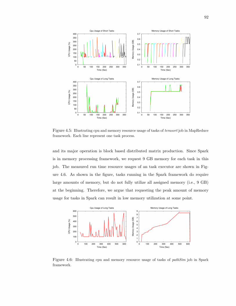
92

0

50

100

150

200

250

300

350

400

0 50 100 150 200 250 300 350C

PU

Usa

ge

(%

)Time (Sec)

Cpu Usage of Short Tasks

0.1

0.2

0.3

0.4

0.5

0.6

0.7

0 50 100 150 200 250 300 350

Me

mo

ry U

sa

ge

(G

B)

Time (Sec)

Memory Usage of Short Tasks

0

50

100

150

200

250

300

350

400

0 50 100 150 200 250 300 350

CP

U U

sa

ge

(%

)

Time (Sec)

Cpu Usage of Long Tasks

0.1

0.2

0.3

0.4

0.5

0.6

0.7

0 50 100 150 200 250 300 350

Me

mo

ry U

sa

ge

(G

B)

Time (Sec)

Memory Usage of Long Tasks

Figure 4.5: Illustrating cpu and memory resource usage of tasks of terasort job in MapReduceframework. Each line represent one task process.

and its major operation is block based distributed matrix production. Since Spark

is in memory processing framework, we request 9 GB memory for each task in this

job. The measured run time resource usages of an task executor are shown in Fig-

ure 4.6. As shown in the figure, tasks running in the Spark framework do require

large amounts of memory, but do not fully utilize all assigned memory (i.e., 9 GB)

at the beginning. Therefore, we argue that requesting the peak amount of memory

usage for tasks in Spark can result in low memory utilization at some point.

0

100

200

300

400

500

600

0 100 200 300 400 500 600

CP

U U

sa

ge

(%

)

Time (Sec)

Cpu Usage of Long Tasks

0

1

2

3

4

5

6

7

8

9

0 100 200 300 400 500 600

Me

mo

ry U

sa

ge

(G

B)

Time (Sec)

Memory Usage of Long Tasks

Figure 4.6: Illustrating cpu and memory resource usage of tasks of pathSim job in Sparkframework.

93

4.2.1.3 Improve System Resource Utilization

The above results give us some implications that time series resource demand val-

ues might be used for resource allocation, which unfortunately is not practical. It is

difficult to accurately predict actual resource usages of tasks running in many frame-

works. It can also greatly increase complexity of task scheduling even if a precise

prior knowledge is available. Our solution to solving this problem is on-line moni-

toring actual resource usages of all running tasks, and opportunistically scheduling

tasks, i.e., reassign idle resources which have been assigned but not fully utilized by

running tasks. There are two major issues need to be addressed: (1) which tasks are

eligible for opportunistic scheduling, and (2) how to mitigate the impact of possible

resource contentions caused by opportunistic scheduling.

0

1

2

3

4

5

6

7

8

9

0 200 400 600 800 1000 1200

Me

mo

ry U

sa

ge

(G

B)

Time (Sec)

Memory Usage of Each Task

0

20

40

60

80

100

0 200 400 600 800 1000 1200

iow

ait (

%)

Time (Sec)

IO Waits on Slave Node

0

1

2

3

4

5

6

7

8

0 1000 2000 3000 4000 5000

Me

mo

ry U

sa

ge

(G

B)

Time (Sec)

Memory Usage of Each Task

0

20

40

60

80

100

0 1000 2000 3000 4000 5000 6000

iow

ait (

%)

Time (Sec)

IO Waits on Slave Node

Figure 4.7: Illustrating memory resource usage of tasks and system iowait on one clusternode. (1) The upper row represents normal assignment results. Scheduler reserves resourcesaccording to task requests, i.e., peak resource usage of task, for running tasks. Two Sparkjobs therefore run sequentially due to the resource limit of system. (2) The lower row rep-resents opportunistic assignment results. Scheduler assigns tasks whenever there are enoughfree resources on node. Two Spark jobs run concurrently and result in severe performancedegradation when they start competing for memory resources.

We thus first investigate the impact of opportunistic scheduling on performance.

We setup a YARN cluster with 2 slave nodes, each has 12 cores and 44 GB memory,

94

and submit two pathSim jobs with 8 executor tasks, each has 9 GB memory request.

When we set the memory request for each task as 9 GB, only 4 tasks (or executors)

can be launched on each slave node, because the remaining memory available on each

node, 8 GB in this case, is not enough for running any tasks. Therefore, job 2 has to

wait till job 1’s tasks finish and release their resources. Figure 4.7(a)-(b) shows run-

time memory usages of tasks running on one of the slave nodes as well as iowait ratios

of that node. Each task takes around 10 minutes to finish and makespan of these two

jobs is around 21 minutes. No resource contention exists in this case since each task is

guaranteed to maintain their requested resource amount, i.e., 9 GB memory, during

the entire period of their execution. To better utilize system resource, we can adopt

opportunistic scheduling scheme (i.e., launching task to a slave node based on that

node’s present actual resource utilization). Under this scheme, ResourceManager can

schedule tasks from job 2 shortly after job 1 starts, because job 1’s tasks have low

memory usages at the beginning, see figure 4.7(c). Once ResourceManager detects

idle memory resources on a node, it assigns available memory to tasks of job 2.

However, when all running tasks from both jobs need more memory, the total demand

of memory resource exceeds overall memory capacity and thus no tasks can get enough

memory for execution. Additionally, such memory contention further increases I/Os

for swapping, which severely degrades the performance and will eventually cause task

failures. 3

Typically, we can avoid such resource contention in two ways: (1) suspend or (2)

kill tasks that are launched through opportunistic scheduling when detect resource

contention. The discussion on pausing and resuming tasks in Hadoop MapReduce

has been presented in [69]. Despite suspending tasks can save the efforts on task

processing compared with killing tasks, it requires non-negligible extra system design

work. Preservation of task status is application and framework dependent, which

requires considerable disbursements for cluster computing environments that support

a variety of frameworks. Furthermore, it is also not trivial to find right times for task

resuming or find appropriate target nodes for migration especially in the highly dy-

namic cluster computing environments. Therefore, we choose to kill opportunistically3Tasks do not fail immediately when lacking memory in this case since Spark framework has fault

tolerant scheme within each executor.

95

scheduled tasks in order to relief resource contention and performance degradation.

This solution is simple and straight forward, especially, the fault tolerant schemes

in current frameworks can well support automatic re-submission of killed and failed

tasks.

Moreover, simply and randomly choosing tasks for killing does not work either,

it can waste work and weakens the benefit of utilizing idle resources through oppor-

tunistic scheduling tasks. We repeat the previous experiment with submitting the

same two pathSim jobs to the cluster and introduce contention relief scheme which

kills opportunistically launched tasks when detecting memory resource contention.

Memory utilization of running tasks are shown in figure 4.8. In this case, job 2’s tasks

are opportunistically scheduled with job 1’s tasks when they have low memory usage

at the beginning. However, opportunistically scheduled tasks from job 2 are gradu-

ally killed after running for more than 8 minutes when normal assigned tasks from

job 1 are requiring more memory resources, see time period 400-600 in Figure 4.8(a).

As a result, job 1’s execution is delayed (takes more than 700 seconds in this case

compared with 600 seconds when running along as shown in Figure 4.7(a)) due to

performance interference caused by opportunistically launched tasks, and execution

of job 2’s opportunistically launched tasks are totally wasted. Moreover, job 2’s tasks

are killed again since all of its 8 tasks have been packed into the same machine after

job 1 finished, see time period around 1000 in Figure 4.8(a). Under such case, al-

though cluster memory resources are fully utilized, no jobs benefit from opportunistic

scheduling since the waste of work surpass the increase of resource utilization.

0

1

2

3

4

5

6

7

8

9

0 200 400 600 800 1000

Me

mo

ry U

sa

ge

(G

B)

Time (Sec)

Memory Usage of Each Task

0

20

40

60

80

100

0 200 400 600 800 1000

iow

ait (

%)

Time (Sec)

IO Waits on Slave Node

Figure 4.8: Illustrating memory resource usage of tasks and system iowait on one cluster nodeunder opportunistically scheduling. Task killing is performed to avoid memory contention.

To solve this problem, we only consider tasks that have short life times for oppor-

96

tunistic scheduling. Such opportunistically launched tasks can finish soon and return

occupied resources to eliminate resource contention; and killing these tasks will not

waste a significant amount of work. Our proposed opportunistic scheduling scheme is

practical and effective due to the following characteristics of cluster computing frame-

works. First, most tasks in cluster computing frameworks, e.g., MapReduce tasks [27],

are short, which gives us a good chance of opportunistic scheduling. Second, it is

highly possible to predict task lengths in most cluster computing frameworks. Jobs in

these cluster computing frameworks usually consist of multiple stages, each of which

has tasks with identical functionality to process a similar amount of data. It follows

that each stage’s tasks usually have similar life times, e.g., as shown in Figure 4.5,4.7,

many tasks (represented by lines) have similar execution length. With an accurate

prediction mechanism, it is guaranteed that killing opportunistic scheduled tasks has

minimum negative effect on overall system performance.

4.2.2 Opportunistic Scheduling - Design and Implementation

In this section, we present a new scheme named OpRM, which aims to improve the

system resource utilization as well as throughput of current cluster computing frame-

works. In particular, we implement our scheme on top of Hadoop YARN resource

management framework and its FAIR scheduling policy.

4.2.2.1 Architecture

Client

ResourceManager

NodeManager NodeManager

Job Submission

Task/Resource

Status

Resource

Request/Assignment

Task Launching

Figure 4.9: Demonstrating the architecture of opportunistic scheduling on YARN. Darkcomponents are modified or new designed modules.

97

Table 4.3: Notations used in this work.ni working node iRc

i / Rai resource capacity / available resources on node i

Rgi / Ro

i guaranteed / opportunistic available resources on node iTTT i / TTTn

i set of total assigned / normal assigned tasks on node itr / tn reserved / next available taskRd

t / Rat resource demand / actual resurce usage of task t

Rbi / T b

i blocked resources / time period on node i

The architecture of our design upon YARN framework is shown in figure 4.9. We

mainly introduce the following three components to the existing YARN framework:

• Opportunistic Scheduler: Makes scheduling decisions for pending tasks;

• Task Classifier: Classifies pending tasks into short or long task categories;

• Monitor: Tracks and reports run-time resource utilizations of running tasks.

Performs contention relief policy to prevent performance interference when de-

tects resource contention on node;

Once an application is submitted to YARN system by a client, a special task called

ApplicationMaster (AM) will first be launched. AM requires resources for all re-

maining tasks of the application from the ResourceManager (RM). Task requests are

classified into two categories, i.e., short and long, and labeled by the Task Classifier.

Opportunistic Scheduler maintains all waiting task requests in queues, and performs

task scheduling whenever receives heartbeat message from a NodeManager which

reports status of node and running tasks on node. Monitors running on each Node-

Manager monitor and report run-time utilizations of running tasks to Opportunistic

Scheduler through heartbeat messages. Furthermore, Monitors are also responsible

for preventing performance interference caused by opportunistic scheduling. Details

of these components are discussed in the following sections. Summary of notations

used in this section is listed in table 4.3.

4.2.2.2 Opportunistic schedule

As discussed in Section 4.2.1, tasks do not always fully utilize their assigned resources

during their lifetime. However, the ResourceManager under current YARN framework

estimates the amount of residual resource on each working node as the gap between

98

the node resource capacity and the summation of resource demands of tasks running

on it, see equation 4.7. Consequently, idle resources on a node might be more than

the estimated available resources, which can incur low resource utilization.

Rai = Rci − Σt∈TTT iRdt ; (4.7)

To address this issue, we design the opportunistic scheduler, which considers two kinds

of available resources, i.e., guaranteed available resources (Rg), and opportunistic

available resources (Ro), for managing and assigning resources. In particular, Oppor-

tunistic Scheduler always guarantees the assigned amount of resources are available

during a task’s lifetime if that task is assigned with guaranteed available resources.

We refer to this kind of resource assignment as normal assignment/schedule. On the

other hand, a task might lose its assigned opportunistic available resources before

it finishes. We refer to it as opportunistic assignment/schedule. Rg and Ro of each

working node are calculated in different ways as shown in equation 4.8-4.9. Rgi is equal

to the difference between node i’s resource capacity Rci and the resource demands of

normal assigned tasks that are currently running on node i. While, the calculation of

Roi is based on actual resource usages of all active tasks on node i. Since running tasks

may have lower actual resource usage than their resource demands in idle periods,

Opportunistic scheduler can then use Ro to further capture and utilize those reserved

but idle resources.

Rgi = Rci − Σt∈TTTniRdt ; (4.8)

Roi = Rci − Σt∈TTT iRat ; (4.9)

Algorithm 4.2 presents the high level idea of our scheduling scheme 4. As discussed

in section 4.2.2.1, NodeManager of each working node periodically sends heartbeat

messages to ResourceManager, which includes node health status and run-time re-

source utilizations of each running task. When receiving heartbeat message from one

working node, opportunistic scheduler updates the guaranteed/opportunistic avail-

able resources of that node through equation 4.8-4.9, see line 2-3. The next waiting

task requirement is chosen for assignment from the waiting queues according to user4We implement the opportunistic scheduler based on the FAIR scheduling policy. Note it can

also be integrated with any other scheduling algorithms.

99

defined scheduling policy, e.g., FAIR, see line 10-14. When trying to assign available

resources of node, opportunistic scheduler always first tries to assign guaranteed avail-

able resources, i.e., normal assign, see line 15-17. If resource demand of the chosen

task does not fit into the guaranteed available resources of node, scheduler will try op-

portunistic assignment, see line 18-19. If the task is still not eligible for opportunistic

scheduling or cannot fit into the opportunistic available resources on node, scheduler

reserves this task on the node and stops the assignment process until receiving next

heartbeat message, see line 20-23. Only one task can be reserved on each node, and

the reserved task has a higher priority for assignment, see line 6-9.

In summary, the key difference between the existing scheduler and our proposed

opportunistic scheduler lies in the approach of estimating and assigning available re-

sources on node. Existing schedulers only consider to assign available resources which

have not been reserved for any tasks, i.e., guaranteed available resources. Oppor-

tunistic scheduler instead considers all available resources, including the assigned but

not used resources, aiming to improve system efficiency. In the following section, we

will discuss how to classify waiting tasks, i.e., determine which tasks are eligible for

opportunistic assignment.

4.2.2.3 Task Classifier

In this work, we classify tasks into two categories, i.e., short and long. Our oppor-

tunistic scheduler thus only considers short tasks for opportunistic scheduling, such

that they have a high chance to finish their work before opportunistic assigned re-

sources vanish and killing these opportunistic assigned short tasks due to resource

contention does not incur a significant waste of work. We expect that by this way,

idle resources that have yet been assigned or reserved can be effectively reused by

other waiting tasks.

One of the issues that need to be addressed is how we can accurately classify

a task that is waiting in the system. We claim that execution length of tasks in

cluster computing frameworks are predictable. The reason is that tasks from the

same stage of an application usually have identical function and process similar size

of input data and thus have similar execution length. For example, a wordcount

MapReduce application that processes 10GB input data has 80 mapper tasks, each

100

processes 128MB input data chunk (when the HDFS is configured with 128MB block

size), and all these 80 mapper tasks have similar execution times. Another wordcount

MapReduce application that processes 100GB input data should have 800 mapper

tasks when submitted to the same YARN cluster. Each mapper task still has 128MB

input size and thus has similar task execution time compared with mapper tasks in

the application that processes 10GB input data. Therefore, we can predict task length

based on historical informations. The challenges of accurate task length classification

here are (1) scheduler can only get very limited information from a submitted task

request; and (2) how do we classify tasks when there is no historical information, e.g.,

a new type of application.

Our scheme adopts naive Bayes classifier [61] to identify tasks as short or long. It

has been widely used in text classification and spam filtering due to its high accuracy

and low overhead on both storage and computation. And we address the challenges

of task classification in cluster computing frameworks by presenting a new hierarchy

approach that considers the following five properties to select features for each task

t.

• Property 1: the framework (denoted as Ft), e.g., MapReduce, Spark, Storm,

that submits task t;

• Property 2: priority of task t (denoted as St), since tasks in different stages usu-

ally have different priorities in YARN system, this can also be used to determine

the stage a task belongs to;

• Property 3: current progress of the application that submits task t (denoted as

Pt, Pt ⊆ [0, 1]);

• Property 4: application name (denoted as At) of task t;

• Property 5: resource demand of task t (denoted as Rt);

We then define the features of each task t as a tuple using equation 4.10.

Featuret =

{Ft, (Ft, St), (Ft, St, Pt), (Ft, St, Pt, At), (Ft, St, Pt, At, Rt)}; (4.10)

101

The reason for choosing such hierarchy features instead of using task properties sep-

arately are as follows. First, combining these task properties together provides more

meaningful hints for better prediction accuracy. For example, a task t of the fea-

ture (Ft = “MapReduce′′, St = 20) gives the hint that this task is a mapper task in

MapReduce framework5. On the other hand, the task property St = 20 itself does

not convey useful information if considered separately. Furthermore, tasks from the

same type of application but running on different frameworks often have varying life

time. Considering individual task properties like application name cannot help the

classifier getting useful information to distinguish tasks. This may not be a big issue

for classic text classification problem when there are a large number of features, e.g.,

thousands of different vocabularies. However, in our classification criteria, each task

request only provides a limited number of properties, such that each feature has sig-

nificant impact on decisions. Therefore, we decide to combine different task properties

in order to get a set of more meaningful features that help distinguish and classify

tasks. Secondly, the design of hierarchy features can further help our classifier make

reasonable decisions for tasks which are newly met without any historical informa-

tion. For example, when a new MapReduce job is launched, our classifier can classify

its mapper tasks using the historical information of all finished mapper tasks from

different applications but running on the same MapReduce framework.

When a task t’s features (Featuret) are determined, we calculate the posterior

probability (P (C|Featuret)) of its category (Ct) using equations 4.11-4.12 as follows.

P (Ct|Featuret) ∝ P (Ct) ∗ P (Featuret|Ct), (4.11)

P (Featuret|Ct) =∏

P (Featureit|Ct); (4.12)

(4.13)

Where C ∈ {short, long}. Task t will then be classified to one of the two categories

which has a higher posterior probability. Probabilities, e.g., P (Ct), P (Featureit|Ct),

used in equation 4.11-4.12 are on-line learned and updated upon the completion of

tasks. We determine the category (short or long) of finished tasks by checking if their

execution times are less than a threshold (e.g., 1 minute) and update all probabilities5In YARN cluster, all mapper tasks have the task priorities equal to 20, and all reduce tasks have

the task priorities equal to 10.

102

with tasks’ feature and category information. There is a special case when an appli-

cation with new features is submitted. Without any historical information, we opt to

conservatively initialize the probabilities of such features (P (Feature|C)) with bias

to the long category.

4.2.2.4 NodeManager Monitor

The key idea of our new opportunistic scheduling scheme is to assign idle resources

to pending tasks based on actual run time resource usages. Therefore, we imple-

ment and plug a monitor module on NodeManagers to (1) keep tracking both cpu

and memory usages of running tasks and sending the collected usage information to

ResourceManager through heartbeat messages; and (2) detect and solve performance

interferences caused by resource contentions when resources on that node have been

over provisioned and overall resource demand of running tasks exceeds node capacity.

Algorithm 4.3 shows the main process for detecting and mitigating resource con-

tention on a working node. In particular, our resource monitor periodically collects

real-time cpu and memory usage of running tasks, and updates the aggregated cpu and

memory usages Rcpui and Rmemi on the working node ni, see line 1-10. Once Ri(cpu)

or Ri(mem) exceeds a pre-defined threshold (see line 13-19 in Algorithm 4.3) the

monitor identifies possible existence of resource contention on that node and triggers

a mechanism to release some occupied resources to avoid performance interference.

In our experiments, we set the threshold as ρ ∗Rci (cpu) and ρ ∗Rci (mem) for cpu and

memory respectively, and ρ, set to be equal to 0.95 in our experiments, can be used

to adjust the aggressiveness of our scheme.

We consider the following three policies to solve the problem of performance in-

terference caused by resource contention.

• LAZY : this policy only kills the most recently launched task through oppor-

tunistic scheduling when the monitor detects contention on memory resources;

• STRICT : this policy kills the most recently launched task through opportunistic

scheduling when memory or cpu contention has been detected;

• PRESERVE : this policy kills the most recently launched task through oppor-

tunistic scheduling when memory or cpu contention has been detected, and

103

further block certain amount of opportunistic available resources of this node

for a period of time;

LAZY policy, see line 21-23 in algorithm 4.3, only kills tasks to address memory

contentions. This policy ignores cpu contention mainly because cpu contention usually

does not cause task failures as memory contention does. As opportunistic tasks are

short ones and can return occupied resources quickly, the LAZY policy tends to

aggressively keep running these opportunistic tasks even under cpu contentions for

achieving better overall performance. One the other hand, the drawback of this policy

is that normally reserved resources cannot always be guaranteed especially during the

periods of system overload.

In contrast, STRICT is a conservative policy (see line 24-26 of algorithm 4.3) which

kills opportunistic tasks under both cpu and memory resource contention. Clearly,

this policy can guarantee reserved resources but might incur too frequent task termi-

nations, especially when resource utilizations of running tasks are oscillating, e.g., see

figure 4.6.

To avoid killing too many tasks but still guarantee reserved resources, we further

present a new contention relief policy, named PRESERVE, by introducing the con-

cepts of blocked resource (Rbi ) and block time (T bi ), see line 27-37 of algorithm 4.3.

Besides killing opportunistic tasks, this policy further blocks an amount (Rbi ) of re-

sources from opportunistic available resources of node ni for a time window (T bi ).

Under PRESERVE policy, the opportunistic scheduler will estimate opportunistic

available resources (Roi ) by considering both actual resource usage of running tasks

(Rat ) and the amount of blocked resources (Rbi ), see equation 4.14.

Roi = Rci − Σt∈TTT iRat −Rbi ; (4.14)

The values of Rbi and T bi are adjusted with the similar idea of congestion avoidance

algorithm that is used in networking systems. We double the Rbi and T bi values to

be more conservative if a new resource contention is detected within current blocking

time window. Similarly, the values of Rbi and T bi will be decreased exponentially by a

factor of two if no resource contention has been detected in the T bi window. We also

set the minimum/maximum thresholds for both Rbi and T bi , e.g., in our experiments,

we have 0 < Rbi <= 0.5∗Rci and the range of T bi is between 30 seconds and 90 seconds.

104

4.2.3 Evaluation

We implement the proposed opportunistic scheduling scheme OpRM on Hadoop YARN

V2.5. We modified the scheduler part in the ResourceManager of YARN (based on

Fair scheduler in this work) to include a task classifier and to separate normal task

assignment and opportunistic task assignment. In the NodeManager, we enabled run

time resource monitoring and reporting as well as contention detection and relief in

the ContainerMonitor component. The communication protocols and messages be-

tween ResourceManager, NodeManagers, and ApplicationMasters are also modified to

convey the actual resource usage and assignment type (i.e., normal or opportunistic)

information of tasks. We evaluate OpRM in a YARN cluster with different data pro-

cessing workloads which are mixed with representative MapReduce and Spark jobs.

We then present the detailed experimental settings in Section 4.2.3.1 and discuss

experimental results in Section 4.2.3.2.

4.2.3.1 Experiment Settings

We conduct our experiments in a YARN cluster which is deployed in a cloud en-

vironment provided by CloudLab [62]. This YARN cluster is configured with one

master node and 20 working nodes, each of which has 8 physical cores. We configure

2 virtual cores for each physical core. So there are 16 vcores in total on each working

node where we leave 1 vcore for NodeManager and HDFS usage, and the remain-

ing 15 vcores can be used for running cluster computing applications. Each node is

configured with memory capacity of 12 GB.

The following four benchmarks are considered in our experiments:

• pathSim: a Spark application that computes the meta path based similarity [60]

between academic paper authors. Input data is 1.2 million paper submission

records.

• terasort: a MapReduce application that sorts input records, the input 50GB

data is generated through teragen.

• wordcount: a MapReduce application that counts the occurrence of each word

in input files. Each input file with 50GB data is generated through randomTex-

105

tWriter.

• piEstimate: a MapReduce application that estimates the value of π using the

quasi-Monte Carlo method; each task processes 300 million data points.

Table 4.4 shows task configurations of each application, including task numbers

and task resource requests. By default, we configure each task’s resource request

according to their actual resource usage. The cpu demand of a task is equal to 75%

of its peak cpu usage and the memory requirement is set to that task’s maximum

memory usage. These applications thus have various resource requirements. For

example, tasks from Spark applications are memory intensive while MapReduce tasks

are mainly cpu intensive.

4.2.3.2 Experiment Results

We conduct three sets of experiments in a MapReduce YARN cluster to evaluate our

new opportunistic scheduling scheme. In all experiments, we use the results under

the original YARN framework with Fair scheduler as a base line for comparison. The

performance metrics we consider for evaluating the effectiveness of OpRM include

resource utilizations, and job execution times.

Workloads with MapReduce jobs only

In the first set of experiments, we generate a workload which includes a batch of

MapReduce jobs by submitting 2 jobs from each MapReduce application type as

listed in Table 4.4. That is, we run 6 MapReduce jobs in a batch under both original

Fair policy, and our opportunistic scheduler. We further consider three mechanisms,

i.e., LAZY, STRICT, and PRESERVE for contention relief.

The first set of results, shown in Table 4.5, demonstrates the prediction accuracy of

our task classifier which adopts the hierarchy feature-based naive Bayes classification

algorithm as described in Section4.2.2.3. Each entry in Table 4.5 shows how many

short/long tasks are predicted as short or long. We note that the major issue of

our scheme is to avoid false positives, i.e., predicting a long task as short, which can

incur server resource contention or significant work lost up on task killing. On the

other hand, a false negative, i.e., predicting a short task as long, only prevents us

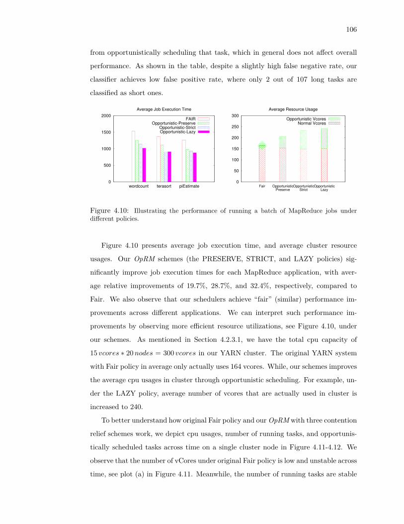
106

from opportunistically scheduling that task, which in general does not affect overall

performance. As shown in the table, despite a slightly high false negative rate, our

classifier achieves low false positive rate, where only 2 out of 107 long tasks are

classified as short ones.

0

500

1000

1500

2000

wordcount terasort piEstimate

Average Job Execution Time

FAIROpportunistic-Preserve

Opportunistic-StrictOpportunistic-Lazy

0

50

100

150

200

250

300

Fair OpportunisticPreserve

OpportunisticStrict

OpportunisticLazy

Average Resource Usage

OpportunisticVcoresNormalVcores

Figure 4.10: Illustrating the performance of running a batch of MapReduce jobs underdifferent policies.

Figure 4.10 presents average job execution time, and average cluster resource

usages. Our OpRM schemes (the PRESERVE, STRICT, and LAZY policies) sig-

nificantly improve job execution times for each MapReduce application, with aver-

age relative improvements of 19.7%, 28.7%, and 32.4%, respectively, compared to

Fair. We also observe that our schedulers achieve “fair” (similar) performance im-

provements across different applications. We can interpret such performance im-

provements by observing more efficient resource utilizations, see Figure 4.10, under

our schemes. As mentioned in Section 4.2.3.1, we have the total cpu capacity of

15 vcores ∗ 20nodes = 300 vcores in our YARN cluster. The original YARN system

with Fair policy in average only actually uses 164 vcores. While, our schemes improves

the average cpu usages in cluster through opportunistic scheduling. For example, un-

der the LAZY policy, average number of vcores that are actually used in cluster is

increased to 240.

To better understand how original Fair policy and our OpRM with three contention

relief schemes work, we depict cpu usages, number of running tasks, and opportunis-

tically scheduled tasks across time on a single cluster node in Figure 4.11-4.12. We

observe that the number of vCores under original Fair policy is low and unstable across

time, see plot (a) in Figure 4.11. Meanwhile, the number of running tasks are stable

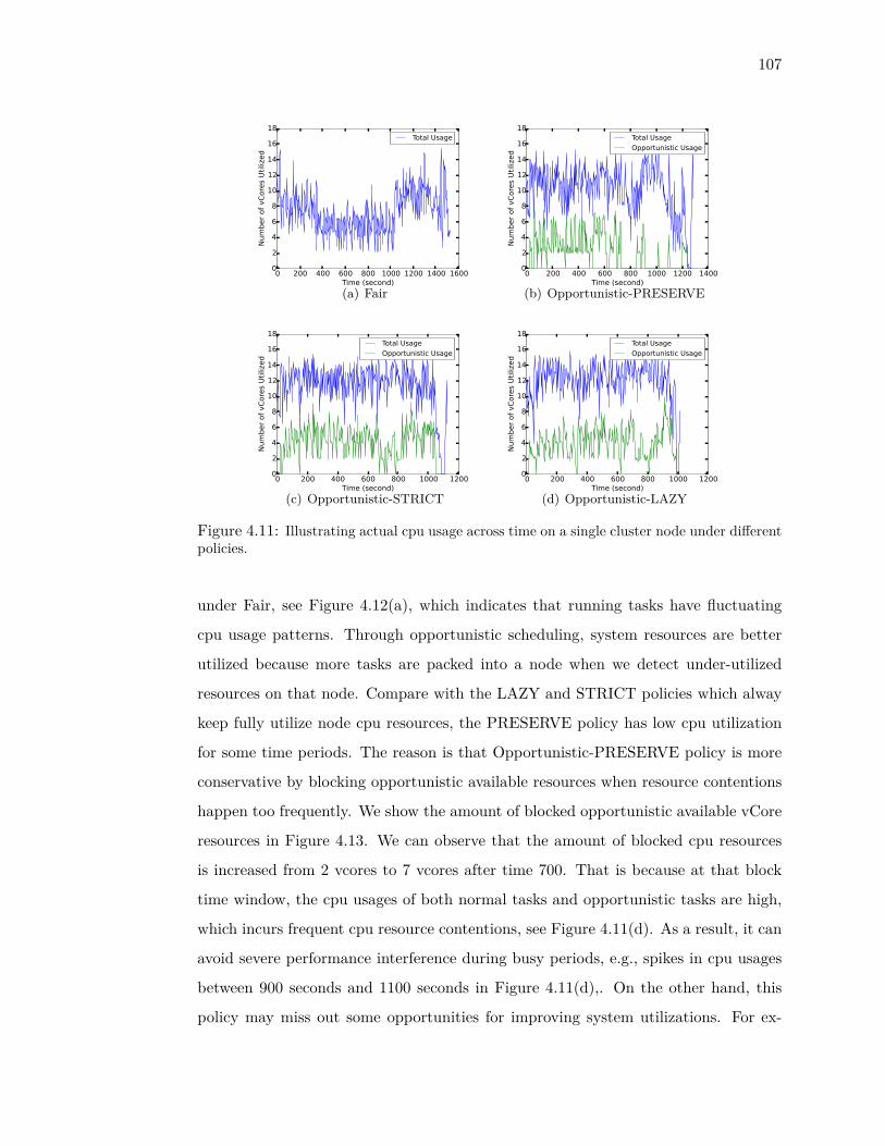
107

0 200 400 600 800 1000 1200 1400 1600Time (second)

0

2

4

6

8

10

12

14

16

18

Numbe

r of v

Cores Utilize

d

Total Usage

(a) Fair0 200 400 600 800 1000 1200 1400

Time (second)0

2

4

6

8

10

12

14

16

18

Numbe

r of v

Cores Ut

ilize

d

Total UsageOpportunistic Usage

(b) Opportunistic-PRESERVE

0 200 400 600 800 1000 1200Time (second)

0

2

4

6

8

10

12

14

16

18

Numbe

r of v

Cores Ut

ilize

d

Total UsageOpportunistic Usage

(c) Opportunistic-STRICT0 200 400 600 800 1000 1200

Time (second)0

2

4

6

8

10

12

14

16

18

Numbe

r of v

Cores Ut

ilize

d

Total UsageOpportunistic Usage

(d) Opportunistic-LAZY

Figure 4.11: Illustrating actual cpu usage across time on a single cluster node under differentpolicies.

under Fair, see Figure 4.12(a), which indicates that running tasks have fluctuating

cpu usage patterns. Through opportunistic scheduling, system resources are better

utilized because more tasks are packed into a node when we detect under-utilized

resources on that node. Compare with the LAZY and STRICT policies which alway

keep fully utilize node cpu resources, the PRESERVE policy has low cpu utilization

for some time periods. The reason is that Opportunistic-PRESERVE policy is more

conservative by blocking opportunistic available resources when resource contentions

happen too frequently. We show the amount of blocked opportunistic available vCore

resources in Figure 4.13. We can observe that the amount of blocked cpu resources

is increased from 2 vcores to 7 vcores after time 700. That is because at that block

time window, the cpu usages of both normal tasks and opportunistic tasks are high,

which incurs frequent cpu resource contentions, see Figure 4.11(d). As a result, it can

avoid severe performance interference during busy periods, e.g., spikes in cpu usages

between 900 seconds and 1100 seconds in Figure 4.11(d),. On the other hand, this

policy may miss out some opportunities for improving system utilizations. For ex-

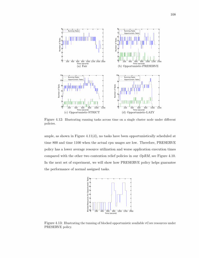
108

0 200 400 600 800 1000 1200 1400 1600Time (second)

0

1

2

3

4

5

6

7

8

Numbe

r of Tasks

Running Tasks

(a) Fair0 200 400 600 800 1000 1200 1400

Time (second)0

1

2

3

4

5

6

7

8

Number o

f Tasks

Running TasksOpportunistic Tasks

(b) Opportunistic-PRESERVE

0 200 400 600 800 1000 1200Time (second)

0

2

4

6

8

10

12

Numbe

r of Tasks

Running TasksOpportunistic Tasks

(c) Opportunistic-STRICT0 200 400 600 800 1000 1200

Time (second)0

2

4

6

8

10

Numbe

r of Tasks

Running TasksOpportunistic Tasks

(d) Opportunistic-LAZY

Figure 4.12: Illustrating running tasks across time on a single cluster node under differentpolicies.

ample, as shown in Figure 4.11(d), no tasks have been opportunistically scheduled at

time 800 and time 1100 when the actual cpu usages are low. Therefore, PRESERVE

policy has a lower average resource utilization and worse application execution times

compared with the other two contention relief policies in our OpRM, see Figure 4.10.

In the next set of experiment, we will show how PRESERVE policy helps guarantee

the performance of normal assigned tasks.

0 200 400 600 800 1000 1200 1400Time (second)

0

1

2

3

4

5

6

7

8

Bloc

ked Re

source

s For O

pportunistic Ta

sks

Figure 4.13: Illustrating the tunning of blocked opportunistic available vCore resources underPRESERVE policy.

109

Workloads with Mixed MapReduce and Spark jobs

In the second set of experiments, we launch two Spark jobs, i.e., pathSim, to the clus-

ter, such that Spark executors will occupy 10 GB (9 GB executor memory request and

1 GB overhead) memory capacity of each cluster node. We then submit a batch of 6

MapReduce jobs (same configuration with the first experiment sets) to run in parallel

with the Spark jobs. Experiment results are shown in Figure 4.14. MapReduce jobs

receive significant performance boost in this set of experiments. Average job execu-

tion time of all MapReduce jobs is improved by 25.5%, 29.3%, and 36.1% respectively

under the PRESERVE, STRICT, and LAZY policies. On the other hand, Spark

jobs, i.e., pathSim, do not benefit from opportunistic scheduling. The reason is that

Spark jobs have few tasks, and all tasks can be finished in a single wave. Therefore,

the parallelism of Spark tasks cannot be further improved for better job execution

time. The performance of Spark jobs is even worse under opportunistic scheduling

due to the resource contentions caused by opportunistic scheduling. The degradation

is 2.7%, 5.4%, and 6.3% respectively under our proposed three contention relief poli-

cies. Although have lower system utilization level, PRESERVE policy achieves better

performance isolation for normal assigned tasks (i.e., tasks from Spark framework)

compared with other two contention relief policies. Moreover, compared with STRICT

policy which simply kills tasks when detect resource contention, PRESERVE policy

performs task killing much less often. Figure 4.15 depicts the number of killed tasks

and the amount of wasted workloads across time under PRESERVE and STRICT

policies on a single cluster node. The total killed task number and wasted workload

length in cluster is 626 and 4270.8 seconds under STRICT policy, while they drop to

246 and 1752.3 seconds respectively under PRESERVE policy.

Workloads with Mixed MapReduce jobs and Spark jobs with sleeping pe-

riods

Finally, we show that our proposed scheme can achieve even better performance im-

provements when tasks have longer idle periods. For example, tasks from interactive

jobs or tasks that process streaming input data may have more frequent and longer

idle periods when they are waiting for user inputs or incoming data streams. To

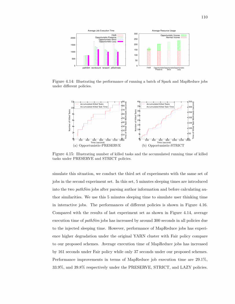
110

0

500

1000

1500

2000

pathSim wordcount terasort piEstimate

Average Job Execution Time

FAIROpportunistic-Preserve

Opportunistic-StrictOpportunistic-Lazy

0

50

100

150

200

250

300

FAIR OpportunisticPreserve

OpportunisticStrict

OpportunisticLazy

Average Resource Usage

OpportunisticVcoresNormalVcores

Figure 4.14: Illustrating the performance of running a batch of Spark and MapReduce jobsunder different policies.

0 200 400 600 800 1000 1200 1400Time (second)

0

2

4

6

8

10

12

Num

ber o

f Kill

ed Ta

sks

Accumulated Killed TasksAccumulated Killed Task Time

0

10

20

30

40

50

60

70

80

90

Tim

e of

Kill

ed Ta

sk W

orkl

oads

(sec

ond)

(a) Opportunistic-PRESERVE0 200 400 600 800 1000 1200 1400

Time (second)0

5

10

15

20

25

30

35

40

Numbe

r of K

illed

Tasks

Accumulated Killed TasksAccumulated Killed Task Time

0

50

100

150

200

250

300

350

Time of Killed

Task W

orkloa

ds (s

econ

d)

(b) Opportunistic-STRICT

Figure 4.15: Illustrating number of killed tasks and the accumulated running time of killedtasks under PRESERVE and STRICT policies.

simulate this situation, we conduct the third set of experiments with the same set of

jobs in the second experiment set. In this set, 5 minutes sleeping times are introduced

into the two pathSim jobs after parsing author information and before calculating au-

thor similarities. We use this 5 minutes sleeping time to simulate user thinking time

in interactive jobs. The performances of different policies is shown in Figure 4.16.

Compared with the results of last experiment set as shown in Figure 4.14, average

execution time of pathSim jobs has increased by around 300 seconds in all policies due

to the injected sleeping time. However, performance of MapReduce jobs has experi-

ence higher degradation under the original YARN cluster with Fair policy compare

to our proposed schemes. Average execution time of MapReduce jobs has increased

by 161 seconds under Fair policy while only 37 seconds under our proposed schemes.

Performance improvements in terms of MapReduce job execution time are 29.1%,

33.9%, and 39.8% respectively under the PRESERVE, STRICT, and LAZY policies.

111

0

500

1000

1500

2000

2500

pathSim wordcount terasort piEstimate

Average Job Execution Time

FAIROpportunistic-Preserve

Opportunistic-StrictOpportunistic-Lazy

0

50

100

150

200

250

300

FAIR OpportunisticPreserve

OpportunisticStrict

OpportunisticLazy

Average Resource Usage

OpportunisticVcoresNormalVcores

Figure 4.16: Illustrating the performance of running Spark jobs with waiting time andMapReduce jobs under different policies.

Figure 4.17 shows the resource utilization across time on one of the cluster nodes

under different policies. As shown in the figure, the node is idle in the first 5 minutes,

i.e., sleeping time of pathSim job, under Fair policy. It is because waiting MapReudce

tasks cannot acquire the occupied resources of running Spark tasks even if they are

not using any of the assigned resources. On the other hand, our proposed scheme

can significantly increase cluster resource utilization and task throughputs through

opportunistic scheduling in such idle periods.

112

0 500 1000 1500 2000Time (second)

0

2

4

6

8

10

Mem

ory Us

age (GB)

Total Usage

(a) Fair0 200 400 600 800 1000 1200 1400

Time (second)0

2

4

6

8

10

12

Mem

ory Us

age (GB)

Total UsageOpportunistic Usage

(b) Opportunistic-PRESERVE

0 500 1000 1500 2000Time (second)

0

2

4

6

8

10

12

14

Numbe

r of v

Cores Utilize

d

Total Usage

(c) Fair0 200 400 600 800 1000 1200 1400

Time (second)0

2

4

6

8

10

12

14

16

18

Numbe

r of v

Cores Ut

ilize

d

Total UsageOpportunistic Usage

(d) Opportunistic-PRESERVE

Figure 4.17: Illustrating actual resource usage across time on one cluster node under differentpolicies.

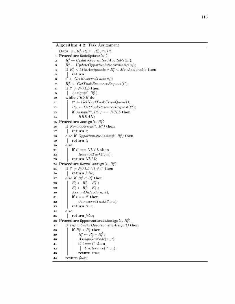
113

Algorithm 4.2: Task AssignmentData: ni, R

gi , R

oi , t

r, Rdtr , tn, Rd

tn

1 Procedure NodeUpdate(ni)2 Rg

i ← UpdateGuaranteedAvailable(ni);3 Ro

i ← UpdateOpportunisticAvailable(ni);4 if Rg

i < MinAssignable ∧Roi < MinAssignable then

5 return6 tr ← GetReservedTask(ni);7 Rd

tr ← GetTaskResourceRequest(tr);8 if tr 6= NULL then9 Assign(tr, Rd

tr );10 while TRUE do11 tn ← GetNextTaskFromQueue();12 Rd

tn ← GetTaskResourceRequest(tn);13 if Assign(tn, Rd

tn ) == NULL then14 BREAK;15 Procedure Assign(t, Rd

t )16 if NormalAssign(t, Rd

t ) then17 return t;18 else if OpportunisticAssign(t, Rd

t ) then19 return t;20 else21 if tr == NULL then22 ReserveTask(t, ni);23 return NULL;24 Procedure NormalAssign(t, Rd

t )25 if tr 6= NULL ∧ t 6= tr then26 return false;27 else if Rd

t < Rgi then

28 Rgi ← Rg

i −Rdt ;

29 Roi ← Ro

i −Rdt ;

30 AssignOnNode(ni, t);31 if t == tr then32 UnreserveTask(tr, ni);33 return true;34 else35 return false;36 Procedure OpportunisticAssign(t, Rd

t )37 if IsEligibleForOpportunisticAssign(t) then38 if Rd

t < Roi then

39 Roi ← Ro

i −Rdt ;

40 AssignOnNode(ni, t);41 if t == tr then42 UnReserve(tr, ni);43 return true;44 return false;

114

Algorithm 4.3: Node MonitoringData: Ri(cpu), Ri(mem),TTT o, Rc

i (cpu), Rci (mem), POLICY,Rb

i , Rb′

i , Tbi

1 Procedure Monitoring()2 while TRUE do3 Ri(cpu)← 0;4 Ri(mem)← 0;5 TTT o ← {};6 foreach t in RunningTasks do7 Ri(cpu)← Ri(cpu) + CurrentCpuUsage(t);8 Ri(mem)← Ri(mem) + CurrentMemoryUsage(t);9 if IsOpportunistic(t) then

10 TTT o ← TTT o ∪ {t}11 Contention← IsContention(Ri(cpu), Ri(mem),TTT o)

ReliefContention(Contention, POLICY );12 SLEEP MonitorInterval;13 Procedure IsContention(Ri(cpu), Ri(mem),TTT o)14 if TTT o 6= {} then15 if Ri(mem) > ρ ∗Rc

i (mem) then16 return Memory;17 if Ri(cpu) > ρ ∗Rc

i (cpu) then18 return Cpu;19 return NONE ;20 Procedure ReliefContention(Contention, POLICY )21 if POLICY == LAZY then22 if Contention == Memory then23 KillMostRecentLaunchedOpportunisticTask()24 if POLICY == STRICT then25 if Contention 6= NONE then26 KillMostRecentLaunchedOpportunisticTask()27 if POLICY == PRESERV E then28 if Contention 6= NONE then29 KillMostRecentLaunchedOpportunisticTask() Rb

i ← Rbi ∗ 2;

30 T bi ← T b

i ∗ 2;31 LastReliefT ime = CurrentT ime;32 else33 if CurrentT ime− LastReliefT ime > tr then34 Rb

i ← Rbi −Rb′

i ;35 Rb′

i ← Rb′

i ∗ 2;36 T b

i ← T bi /2;

37 LastReliefT ime = CurrentT ime;

Table 4.4: Task Configurations of Applications.

Framwork Application Task Number Task RequestSpark pathSim 10 executor < 4vcores, 9GB >

terasort 374 mapper < 4vcores, 1GB >100 reducer < 2vcores, 1GB >

MapReduce wordcount 414 mapper < 4vcores, 1GB >50 reducer < 2vcores, 1GB >

piEstimate 500 mapper < 3vcores, 1GB >1 reducer < 2vcores, 1GB >

115

Table 4.5: Task duration classification results.Classification

Task Number Short LongShort 2777 2417 (87.0%) 360 (13.0%)Long 107 2 (1.9%) 105 (98.1%)

116

4.3 Related Work

The work of Omega [63] provided a high-level overview of two generations of Google’s

cluster management systems. Sparrow [64] considers efficient scheduling for sub-

second parallel jobs in Spark framework. MATRIX proposed in [65] is a distributed

many-task computing execution framework, which utilizes the adaptive work stealing

algorithm to achieve distributed load balancing.

Fine-grained resource management was well studied for Hadoop systems. Through-

putScheduler was proposed by Gupta et al. [66] to improve the performance of het-

erogeneous Hadoop clusters. An explore stage was proposed to learn the resource

requirement of tasks and the capabilities of nodes, and the scheduler could then se-

lect the best node to assign tasks. Polo et al. [67] leveraged job profiling information

to dynamically adjust the number of slots on each node, as well as workload place-

ment across nodes, to maximize the resource utilization of the Hadoop cluster. Our

proposed scheduler, however, does not require any learning phases or job profiles for

scheduling. Therefore, HaSTE is more lightweight and practical.

Schedule tasks with resource and dependency constraints is known as the NP hard

resource constrained project scheduling problem (RCPSP). This problem has been

extensively studied in the past decades by many researchers [56–59]. While in YARN

system, scheduling tasks for MapReduce jobs is very close to the RCPSP problem since

there is also resource and dependency constraints of MapReduce tasks. However,

the difference between the dependency of map/reduce tasks and previous defined

dependency of tasks in projects distinguishes the scheduling problem of MapReduce

jobs. The special dependency between map and reduce phases was studied in recent

works [30] of IBM. They proposed to schedule reduce tasks gradually according to

the progress of map tasks. However, their solution mainly considers the single job

execution situation, and may not be sufficient under resource contention situation in

shared cluster.

Improving resource efficiency and throughput of cluster computing platforms was

extensively studied in recent years. DynMR [68] presents that reduce tasks in MapRe-

duce framework bundle multiple phases and have changing resource utilization, and

propose to assemble multiple reduce tasks into a progressive queue for management

117

and backfill map tasks to fully utilize system resources. Their work is closely bounded

with MapReduce framework, and involves complex task management that cannot be

easily extend to other frameworks. Quasar [14] designs resource efficient and QoS-

aware cluster management. Classification techniques are used to find appropriate

resource allocation to applications to fulfill their QoS requirements and maximize

system resource utilization. Resource assignment in their work is to assign one or

multiple nodes to the application which is different from task assignment in cluster

computing. They mainly address the inefficient resource utilization caused by the gap

between user specified application resource requirements and actual resource usage

of application. While in our work, we mainly address the resource under utilization

caused by fluctuating resource usage pattern of tasks. With the same motivation, work

of [69] enables elastic load balancing and scheduling through pausing or consolidating

idle tasks.

Resource utilization is of greater importance in large enterprise data centers since

increasing utilization by few percents may save a lot in a large scale cluster. Recent

published works reveal some technique details of Google’s Borg system [70] and Mi-

croSoft’s Apollo [71] system. They both have design ideas similar to our work, i.e.,

improve cluster resource utilization by exploring actual resource usage of running jobs

and assign idle resources to pending tasks to improve system utilization. Borg classi-

fies jobs into high priority and low priority categories and monitors resource usage of

high priority tasks and predict their future usage by adding safety margins. If high

priority tasks are not using all their reserved resources, resource manager can reclaim

these resources and assign to low priority tasks. Low priority tasks may be killed or

throttled when high priority tasks require more resources. Apollo starts opportunis-

tic scheduling after all available resource tokens have been assigned to regular tasks.

Fairness is achieved by assigning each job a maximum amount of opportunistic tasks

and randomly select opportunistic tasks from waiting jobs when scheduling. Although

sharing the similar idea, our work differences from their designs in the following as-

pects. Instead of using user defined task priorities or assign each job fixed amount

of opportunistic tasks proportional to job resource tokens, we automatically classify

tasks according to their estimated execution length, and only allow short tasks to be

opportunistic scheduled. Through this classification, the interference introduced by

118

opportunistic scheduling and the penalty of killing unfinished opportunistic tasks are

minimized. With our method, high priority tasks can also benefit from opportunistic

scheduling, and the amount of opportunistic tasks of each job is determined by task

properties instead of job resource requirements. We also design different contention

relief policies and investigate the trade off between them. Different policy can then be

chosen freely according to different situations, e.g., different task latency sensitivity.

119

4.4 Summary

In this chapter, we propose a new scheduler for efficiently schedule MapReduce jobs

in Hadoop YARN system. Our scheduler considers both the fine-grained resource

requirements of tasks and the subtle dependency relationship between tasks while

allocating resources. The proposed scheduler was implemented in the Hadoop YARN

system and evaluated under classic MapReduce workloads. Experiment results re-

veal that our scheduler could improve both the resource utilization of system and the

makespan of a set of MapReduce jobs. We also implement an opportunistic schedul-

ing based scheme for the resource management layer of cluster computing platforms.

In the scheme, we propose to separately consider guaranteed available resources and

opportunistic available resources in cluster. We calculate guaranteed available re-

sources according to each task’s resource demands and get the opportunistic available

resources according to actual task resource usage. We further classify pending tasks

according to their expected running time. By only allowing short tasks for oppor-

tunistic scheduling, we can guarantee that performance interference can be minimized

and killing opportunistic launched tasks will not lead to significant waste. Different

contention relief mechanisms are evaluated through experiments and the results show

great utilization and performance improvements with only slight performance inter-

ference.

120

Chapter 5

Conclusion

In the era of big data, more and more data processing applications have migrated

into cluster computing platforms due to their increasing input size. As the scale of

cluster size and supporting application number grows, there is also increasing impor-

tance of the efficiency of cluster computing platforms. In this dissertation, we mainly

investigated two popular cluster computing platforms, i.e., Hadoop MapReduce and

Hadoop YARN, and aimed to improve their efficiency through more effective resource

management.

We found that current design of Hadoop scheduling and resource management

is not optimized for cluster computing applications since many prominent features

of these applications are not considered. New schedulers and resource management

schemes proposed in this dissertation take advantage of our observed application

properties to improve system efficiency. We developed a job size-based scheduler for

Hadoop MapReduce to improve the average job response time by exploiting the fea-

ture of production Hadoop clusters which usually serve diverse workloads with varying

job sizes. We designed a self-adjusting slot configuration scheme, which is the first

work that uses slot configuration on cluster nodes as a tunable knob to align the

execution of map and reduce phase of consequent MapReduce jobs. Makespan of a

batch of jobs is greatly improved since map and reduce tasks are consuming different

types of system resources and can benefit from pipelined execution. New heuristic

was devised for Hadoop YARN which, to the best of our knowledge, is the only work

that considers both task resource requirements and task dependencies in MapReduce

121

framework for more efficient scheduling. We further proposed opportunistic schedul-

ing approach to more efficiently utilize idle resources in YARN cluster caused by

fluctuating resource usage patterns of cluster computing tasks.

All of the proposed mechanisms in this dissertation are implemented upon open-

sourced Hadoop projects and evaluated with representative workloads. We believe

that our work in this dissertation provides valuable extensions to the existing Hadoop

platforms, which can be easily adopted when system efficiency is a primary concern.

We hope that the designs proposed here can offer a useful reference point of improving

efficiency of cluster computing platforms by exploiting features of cluster computing

applications.

While multiple scheduling policies and resource management schemes were de-

signed for tackling different performance issues in this work, in the future, we plan

to integrate different schemes as an unified solution for Hadoop platform that can

automatically adjust according to user defined performance targets. For example, dif-

ferent scheduling algorithms may be automatically selected for different user queues

according to their primary performance considerations. Furthermore, as the demand

on large-scale data processing grows, new cluster computing platforms are recently

developed to support more complex applications such as iterative machine learning

and graph processing jobs. We also plan to investigate these new cluster computing

applications and platforms and propose more efficient resource management schemes

for these complex applications in the future.

122

Bibliography

[1] J. Dean and S. Ghemawat, “MapReduce: simplified data processing on large

clusters,” Communications of the ACM, vol. 51, no. 1, pp. 107–113, 2008.

[2] A. Thusoo, Z. Shao, S. Anthony, D. Borthakur, N. Jain, J. Sen Sarma, R. Murthy,

and H. Liu, “Data warehousing and analytics infrastructure at facebook,” in Pro-

ceedings of the 2010 ACM SIGMOD International Conference on Management

of data. ACM, 2010, pp. 1013–1020.

[3] T. White, Hadoop: The definitive guide. O’Reilly Media, Inc., 2012.

[4] (2014) Hadoop Users. [Online]. Available: https://wiki.apache.org/hadoop/

PoweredBy

[5] M. Zaharia, M. Chowdhury, M. J. Franklin, S. Shenker, and I. Stoica, “Spark:

cluster computing with working sets,” in Proceedings of the 2nd USENIX con-

ference on Hot topics in cloud computing, 2010, pp. 10–10.

[6] N. Marz, “A storm is coming: more details and plans for release,” Twitter Engi-

neering, vol. 42, 2011.

[7] V. K. Vavilapalli, A. C. Murthy, C. Douglas, S. Agarwal, M. Konar, R. Evans,

T. Graves, J. Lowe, H. Shah, S. Seth et al., “Apache hadoop yarn: Yet another

resource negotiator,” in Proceedings of the 4th annual Symposium on Cloud Com-

puting. ACM, 2013, p. 5.

[8] B. Hindman, A. Konwinski, M. Zaharia, A. Ghodsi, A. D. Joseph, R. H. Katz,

S. Shenker, and I. Stoica, “Mesos: A platform for fine-grained resource sharing

in the data center.” in Unsnix Symposium on Networked Systems Design and

Implementation, vol. 11, 2011, pp. 22–22.

123

[9] A. Thusoo, J. S. Sarma, N. Jain, Z. Shao, P. Chakka, S. Anthony, H. Liu,

P. Wyckoff, and R. Murthy, “Hive: a warehousing solution over a map-reduce

framework,” Proceedings of the VLDB Endowment, vol. 2, no. 2, pp. 1626–1629,

2009.

[10] C. Olston, B. Reed, U. Srivastava, R. Kumar, and A. Tomkins, “Pig latin: a

not-so-foreign language for data processing,” in Proceedings of the 2008 ACM

SIGMOD international conference on Management of data. ACM, 2008, pp.

1099–1110.

[11] R. S. Xin, J. Rosen, M. Zaharia, M. J. Franklin, S. Shenker, and I. Stoica,

“Shark: Sql and rich analytics at scale,” in Proceedings of the 2013 international

conference on Management of data. ACM, 2013, pp. 13–24.

[12] R. S. Xin, J. E. Gonzalez, M. J. Franklin, and I. Stoica, “Graphx: A resilient

distributed graph system on spark,” in First International Workshop on Graph

Data Management Experiences and Systems. ACM, 2013, p. 2.

[13] Y. Chen, A. Ganapathi, R. Griffith, and R. Katz, “The case for evaluating

MapReduce performance using workload suites,” in Modeling, Analysis & Sim-

ulation of Computer and Telecommunication Systems (MASCOTS), 2011 IEEE

19th International Symposium on. IEEE, 2011, pp. 390–399.

[14] C. Delimitrou and C. Kozyrakis, “Quasar: Resource-efficient and qos-aware clus-

ter management,” ACM SIGPLAN Notices, vol. 49, no. 4, pp. 127–144, 2014.

[15] C. Reiss, A. Tumanov, G. R. Ganger, R. H. Katz, and M. A. Kozuch, “Hetero-

geneity and dynamicity of clouds at scale: Google trace analysis,” in Proceedings

of the Third ACM Symposium on Cloud Computing. ACM, 2012, p. 7.

[16] Y. Yao, J. Tai, B. Sheng, and N. Mi, “Lsps: A job size-based scheduler for efficient

assignments in hadoop,” Cloud Computing, IEEE Transactions on, 2014.

[17] ——, “Scheduling heterogeneous MapReduce jobs for efficiency improvement in

enterprise clusters,” in Integrated Network Management, 2013.

124

[18] Y. Yao, J. Wang, B. Sheng, and N. Mi, “Using a tunable knob for reducing

makespan of MapReduce jobs in a hadoop cluster,” in Cloud Computing, IEEE

Transactions on, 2013.

[19] Y. Yao, J. Wang, B. Sheng, C. Tan, and N. Mi, “Self-adjusting slot configurations

for homogeneous and heterogeneous hadoop clusters,” Cloud Computing, IEEE

Transactions on, no. 99, p. 1, 2015.

[20] Y. Yao, J. Wang, B. Sheng, J. Lin, and N. Mi, “Haste: Hadoop yarn schedul-

ing based on task-dependency and resource-demand,” in Cloud Computing

(CLOUD), 2014 IEEE 7th International Conference on. IEEE, 2014, pp. 184–

191.

[21] A. Ghodsi, M. Zaharia, B. Hindman, A. Konwinski, S. Shenker, and I. Sto-

ica, “Dominant resource fairness: Fair allocation of multiple resource types.” in

Proceedings of the 9th USENIX conference on Networked Systems Design and

Implementation, vol. 11, 2011, pp. 24–24.

[22] L. E. Schrage and L. W. Miller, “The queue m/g/1 with the shortest remaining

processing time discipline,” Operations Research, vol. 14, no. 4, pp. pp. 670–684,

1966.

[23] K. Avrachenkov, U. Ayesta, P. Brown et al., “Discriminatory processor shar-

ing revisited,” in IEEE International Conference on Computer Communications,

Mar. 2005, pp. 784–795.

[24] Y. Chen, A. S. Ganapathi, R. Griffith, and R. H. Katz, “A methodology for

understanding MapReduce performance under diverse workloads,” University of

California, Berkeley, Tech. Rep., Nov 2010.

[25] I. Mitrani, Probabilistic Modelling. Cambridge University Press, 1998.

[26] B. Moseley, A. Dasgupta, R. Kumar, and T. Sarlos, “On scheduling in map-

reduce and flow-shops,” in Proceedings of the twenty-third annual ACM sympo-

sium on Parallelism in algorithms and architectures. ACM, 2011, pp. 289–298.

125

[27] S. Kavulya, J. Tan, R. Gandhi, and P. Narasimhan, “An analysis of traces from

a production mapreduce cluster,” in IEEE/ACM International Symposium on

Cluster, Cloud and Grid Computing, 2010, pp. 94–103.

[28] B. P. Welford, “Note on a method for calculating corrected sums of squares and

products,” in Technometrics, 1962, pp. 419–420.

[29] J. Polo, D. Carrera, Y. Becerra, J. Torres, E. Ayguade, M. Steinder, and I. Whal-

ley, “Performance-driven task co-scheduling for mapreduce environments,” in

Network Operations and Management Symposium (NOMS), 2010 IEEE. IEEE,

2010, pp. 373–380.

[30] J. Tan, X. Meng, and L. Zhang, “Performance analysis of coupling scheduler for

mapreduce/hadoop,” in IEEE International Conference on Computer Commu-

nications. IEEE, 2012, pp. 2586–2590.

[31] R. Sumbaly, J. Kreps, and S. Shah, “The big data ecosystem at linkedin,” in

Proceedings of the 2013 international conference on Management of data. ACM,

2013, pp. 1125–1134.

[32] Purdue MapReduce benchmarks suite. [Online]. Available: http://web.ics.

purdue.edu/∼fahmad/benchmarks.htm

[33] Wiki data sets. [Online]. Available: http://dumps.wikimedia.org/

[34] TPC-H benchmark. [Online]. Available: http://www.tpc.org/tpch/

[35] TPC-H benchmark on pig. [Online]. Available: https://issues.apache.org/jira/

browse/PIG-2397

[36] S. M. Johnson, “Optimal two- and three-stage production schedules with setup

times included,” Naval Research Logistics Quarterly, vol. 1, no. 1, pp. 61–68,

1954.

[37] M. Zaharia, D. Borthakur, J. S. Sarma, K. Elmeleegy, S. Shenker, and I. Stoica,

“Job scheduling for multi-user mapreduce clusters,” EECS Department, Univer-

sity of California, Berkeley, Tech. Rep. UCB/EECS-2009-55, 2009.

126

[38] M. Zaharia, D. Borthakur, J. Sen Sarma, K. Elmeleegy, S. Shenker, and I. Stoica,

“Delay scheduling: a simple technique for achieving locality and fairness in cluster

scheduling,” in Proceedings of the 5th European conference on Computer systems.

ACM, 2010, pp. 265–278.

[39] M. Isard, V. Prabhakaran, J. Currey, U. Wieder, K. Talwar, and A. Goldberg,

“Quincy: fair scheduling for distributed computing clusters,” in Proceedings of

the ACM SIGOPS 22nd symposium on Operating systems principles. ACM,

2009, pp. 261–276.

[40] T. Sandholm and K. Lai, “MapReduce optimization using regulated dynamic

prioritization,” ACM SIGMETRICS Performance Evaluation Review, vol. 37,

no. 1, pp. 299–310, 2009.

[41] J. Wolf, D. Rajan, K. Hildrum, R. Khandekar, V. Kumar, S. Parekh, K.-L. Wu,

and A. Balmin, “Flex: A slot allocation scheduling optimizer for mapreduce

workloads,” in ACM/IFIP/USENIX Middleware. Springer, 2010, pp. 1–20.

[42] A. Verma, L. Cherkasova, and R. H. Campbell, “Two sides of a coin: Optimizing

the schedule of mapreduce jobs to minimize their makespan and improve cluster

performance,” in Modeling, Analysis & Simulation of Computer and Telecommu-

nication Systems (MASCOTS), 2012 IEEE 20th International Symposium on.

IEEE, 2012, pp. 11–18.

[43] M. Pastorelli, A. Barbuzzi, D. Carra, M. Dell’Amico, and P. Michiardi, “HFSP:

size-based scheduling for Hadoop,” in Big Data, 2013 IEEE International Con-

ference on. IEEE, 2013, pp. 51–59.

[44] K. Kc and K. Anyanwu, “Scheduling hadoop jobs to meet deadlines,” in Cloud

Computing Technology and Science (CloudCom), 2010 IEEE Second Interna-

tional Conference on. IEEE, 2010, pp. 388–392.

[45] A. Verma, Ludmila Cherkasova, and R. H. Campbell, “ARIA: Automatic re-

source inference and allocation for MapReduce environments,” in IEEE Interna-

tional Conference on Autonomic Computing, 2011, pp. 235–244.

127

[46] L. T. Phan, Z. Zhang, Q. Zheng, B. T. Loo, and I. Lee, “An empirical analysis

of scheduling techniques for real-time cloud-based data processing,” in Service-

Oriented Computing and Applications (SOCA), 2011 IEEE International Con-

ference on. IEEE, 2011, pp. 1–8.

[47] H. Chang, M. Kodialam, R. R. Kompella, T. Lakshman, M. Lee, and S. Mukher-

jee, “Scheduling in mapreduce-like systems for fast completion time,” in IEEE

International Conference on Computer Communications. IEEE, 2011, pp. 3074–

3082.

[48] M. Zaharia, A. Konwinski, A. D. Joseph, R. H. Katz, and I. Stoica, “Improving

mapReduce performance in heterogeneous environments.” in USENIX Sympo-

sium on Operating Systems Design and Implementation, vol. 8, no. 4, 2008, p. 7.

[49] Q. Chen, D. Zhang, M. Guo, Q. Deng, and S. Guo, “Samr: A self-adaptive

mapreduce scheduling algorithm in heterogeneous environment,” in Computer

and Information Technology (CIT), 2010 IEEE 10th International Conference

on. IEEE, 2010, pp. 2736–2743.

[50] C. Tian, H. Zhou, Y. He, and L. Zha, “A dynamic mapreduce scheduler for

heterogeneous workloads,” in Grid and Cooperative Computing, 2009. GCC’09.

Eighth International Conference on. IEEE, 2009, pp. 218–224.

[51] Y. Kwon, M. Balazinska, B. Howe, and J. Rolia, “Skewtune: mitigating skew

in mapreduce applications,” in Proceedings of the 2012 ACM SIGMOD Interna-

tional Conference on Management of Data. ACM, 2012, pp. 25–36.

[52] F. Ahmad, S. T. Chakradhar, A. Raghunathan, and T. Vijaykumar, “Tarazu:

optimizing mapreduce on heterogeneous clusters,” in ACM SIGARCH Computer

Architecture News, vol. 40, no. 1. ACM, 2012, pp. 61–74.

[53] G. Ausiello, Complexity and Approximability Properties: Combinatorial Opti-

mization Problems and Their Approximability Properties. Springer, 1999.

[54] V. V. Vazirani, Approximation algorithms. springer, 2001.

[55] R. Panigrahy, K. Talwar, L. Uyeda, and U. Wieder, “Heuristics for vector bin

packing,” research. microsoft. com, 2011.

128

[56] J. Blazewicz, J. K. Lenstra, and A. Kan, “Scheduling subject to resource con-

straints: classification and complexity,” Discrete Applied Mathematics, vol. 5,

no. 1, pp. 11–24, 1983.

[57] P. Brucker, A. Drexl, R. Mohring, K. Neumann, and E. Pesch, “Resource-

constrained project scheduling: Notation, classification, models, and methods,”

European Journal of Operational Research, vol. 112, no. 1, pp. 3–41, 1999.

[58] T. R. Browning and A. A. Yassine, “Resource-constrained multi-project schedul-

ing: Priority rule performance revisited,” International Journal of Production

Economics, vol. 126, no. 2, pp. 212–228, 2010.

[59] R. Kolisch and S. Hartmann, Heuristic algorithms for the resource-constrained

project scheduling problem: Classification and computational analysis. Springer,

1999.

[60] Y. Sun, J. Han, X. Yan, P. S. Yu, and T. Wu, “Pathsim: Meta path-based

top-k similarity search in heterogeneous information networks,” International

Conference on Very Large Data Bases, 2011.

[61] S. J. Russell, P. Norvig, and S. Chakrabarti, “Artificial intelligence: a modern

approach.”

[62] Cloudlab. [Online]. Available: http://cloudlab.us/

[63] M. Schwarzkopf, A. Konwinski, M. Abd-El-Malek, and J. Wilkes, “Omega: flex-

ible, scalable schedulers for large compute clusters,” in Proceedings of the 8th

ACM European Conference on Computer Systems. ACM, 2013, pp. 351–364.

[64] K. Ousterhout, P. Wendell, M. Zaharia, and I. Stoica, “Sparrow: distributed,

low latency scheduling,” in Proceedings of the Twenty-Fourth ACM Symposium

on Operating Systems Principles. ACM, 2013, pp. 69–84.

[65] K. Wang, X. Zhou, T. Li, D. Zhao, M. Lang, and I. Raicu, “Optimizing load

balancing and data-locality with data-aware scheduling,” in Big Data (Big Data),

2014 IEEE International Conference on. IEEE, 2014, pp. 119–128.

129

[66] S. Gupta, C. Fritz, B. Price, R. Hoover, J. de Kleer, and C. Witteveen,

“ThroughputScheduler: Learning to schedule on heterogeneous hadoop clusters,”

in Proceedings 10th ACM International Conference on Autonomic Computing

(ICAC’13). ACM.

[67] J. Polo, C. Castillo, D. Carrera et al., “Resource-aware adaptive scheduling for

mapreduce clusters,” in ACM/IFIP/USENIX Middleware. Springer, 2011, pp.

187–207.

[68] J. Tan, A. Chin, Z. Z. Hu, Y. Hu, S. Meng, X. Meng, and L. Zhang, “DynMR:

Dynamic mapreduce with reducetask interleaving and maptask backfilling,” in

Proceedings of the Ninth European Conference on Computer Systems. ACM,

2014, p. 2.

[69] G. Ananthanarayanan, C. Douglas, R. Ramakrishnan, S. Rao, and I. Stoica,

“True elasticity in multi-tenant data-intensive compute clusters,” in Proceedings

of the Third ACM Symposium on Cloud Computing. ACM, 2012, p. 24.

[70] A. Verma, L. Pedrosa, M. Korupolu, D. Oppenheimer, E. Tune, and J. Wilkes,

“Large-scale cluster management at google with borg,” in Proceedings of the

Tenth European Conference on Computer Systems. ACM, 2015, p. 18.

[71] E. Boutin, J. Ekanayake, W. Lin, B. Shi, J. Zhou, Z. Qian, M. Wu, and L. Zhou,

“Apollo: scalable and coordinated scheduling for cloud-scale computing,” in Pro-

ceedings of the 11th USENIX conference on Operating Systems Design and Im-

plementation. USENIX Association, 2014, pp. 285–300.