Response of the Indian Ocean Basin Mode and Its …iprc.soest.hawaii.edu/users/xie/iob-change-jc11.pdfResponse of the Indian Ocean Basin Mode and Its Capacitor Effect to Global Warming*

Response of the Indian Ocean Basin Mode and Its Capacitor Effect toGlobal Warming*

XIAO-TONG ZHENG

Physical Oceanography Laboratory, Ocean–Atmosphere Interaction and Climate Laboratory,

Ocean University of China, Qingdao, China

SHANG-PING XIE

International Pacific Research Center, and Department of Meteorology, School of Ocean and Earth Science and Technology,

University of Hawaii at Manoa, Honolulu, Hawaii, and Physical Oceanography Laboratory, Ocean–Atmosphere

Interaction and Climate Laboratory, Ocean University of China, Qingdao, China

QINYU LIU

Physical Oceanography Laboratory, Ocean–Atmosphere Interaction and Climate Laboratory,

Ocean University of China, Qingdao, China

(Manuscript received 26 October 2010, in final form 6 May 2011)

ABSTRACT

The development of the Indian Ocean basin (IOB) mode and its change under global warming are in-

vestigated using a pair of integrations with the Geophysical Fluid Dynamics Laboratory Climate Model

version 2.1 (CM2.1). In the simulation under constant climate forcing, the El Nino–induced warming over the

tropical Indian Ocean (TIO) and its capacitor effect on summer northwest Pacific climate are reproduced

realistically. In the simulation forced by increased greenhouse gas concentrations, the IOB mode and its

summer capacitor effect are enhanced in persistence following El Nino, even though the ENSO itself weakens

in response to global warming. In the prior spring, an antisymmetric pattern of rainfall–wind anomalies and

the meridional SST gradient across the equator strengthen via increased wind–evaporation–sea surface

temperature (WES) feedback. ENSO decays slightly faster in global warming. During the summer following

El Nino decay, the resultant decrease in equatorial Pacific SST strengthens the SST contrast with the en-

hanced TIO warming, increasing the sea level pressure gradient and intensifying the anomalous anticyclone

over the northwest Pacific. The easterly wind anomalies associated with the northwest Pacific anticyclone

in turn sustain the SST warming over the north Indian Ocean and South China Sea. Thus, the increased

TIO capacitor effect is due to enhanced air–sea interaction over the TIO and with the western Pacific. The

implications for the observed intensification of the IOB mode and its capacitor effect after the 1970s are

discussed.

1. Introduction

El Nino–Southern Oscillation (ENSO) is the first

mode of ocean–atmospheric interaction in the equatorial

Pacific. ENSO not only dominates in the tropical Pacific

region but also influences the climate of other regions.

As a remote impact of El Nino, positive anomalies of sea

surface temperature develop over the tropical Indian

Ocean (TIO) during the winter of the developing year of

El Nino, reach the peak in the following spring (Klein

et al. 1999; Alexander et al. 2002; Lau and Nath 2003;

Schott et al. 2009), and persist through boreal summer

(Du et al. 2009). This basinwide warming phenomenon

emerges as the first empirical orthogonal function of

Indian Ocean SST both in observations and model sim-

ulations (Saji et al. 2006; Du et al. 2009; Deser et al. 2010)

and is referred to as the Indian Ocean basin (IOB) mode

in Yang et al. (2007). Yang et al. (2007) and Li et al.

* International Pacific Research Center Publication Number

797.

Corresponding author address: Xiao-Tong Zheng, College of

Physical and Environmental Oceanography, Ocean University of

China, Qingdao 266100, China.

E-mail: [email protected]

6146 J O U R N A L O F C L I M A T E VOLUME 24

DOI: 10.1175/2011JCLI4169.1

� 2011 American Meteorological Society

(2008) suggest that this prolonged basinwide warming is

not simply a passive response to El Nino, but influences

climate like a capacitor in the summer when El Nino has

dissipated. Specifically the IOB mode anchors an anom-

alous anticyclone over the northwest Pacific (NWP) via

atmospheric Kelvin waves and increases mei-yu–baiu

rainfall over East Asia in boreal summer (Xie et al.

2009). In a coupled forecast model, the IOB mode ac-

counts for about 50% of atmospheric anomalies over

NWP during June–August [JJA(1)] (Chowdary et al.

2011a) [numerals in the parentheses denote the ENSO

developing (0) and decay (1) years]. Furthermore, the

TIO warming also suppresses NWP tropical cyclones in

the summer following El Nino (Du et al. 2011).

There are numerous studies that investigate mecha-

nisms for the IOB mode formation. Klein et al. (1999)

show that much of the IOB mode is caused by ENSO-

induced surface heat flux anomalies, including the wind-

induced latent heat flux and solar radiation flux due to

suppressed atmospheric convection over the TIO. Fur-

thermore, a tropospheric temperature (TT) mechanism

is proposed to explain the formation of the IOB mode

(Chiang and Sobel 2002; Chiang and Lintner 2005):

Because of the increased tropospheric temperature over

the tropics during El Nino (Yulaeva and Wallace 1994),

the temperature and humidity of the atmospheric bound-

ary layer over deep convection regions rise, thereby in-

creasing the SST via turbulent heat flux. In the tropical

southwest IO (SWIO) however, the warming cannot be

explained by surface fluxes (Klein et al. 1999), for which

ocean dynamics are important (Xie et al. 2002; Huang

and Kinter 2002). In the developing and mature phases

of El Nino, there are anticyclonic wind anomalies over

the southern TIO, which force a downwelling Rossby

wave (Masumoto and Meyers 1998). The Rossby wave

propagates westward to the SWIO where the mean

thermocline is shallow, deepens the thermocline, and

raises SST (Xie et al. 2002).

Recent studies suggest that the IOB mode is not

uniform in space but shows spatial variations. A series of

TIO–atmosphere interactions helps the IOB mode per-

sist through the summer and shapes its spatiotemporal

structures. In boreal spring, the SWIO warming induces

an antisymmetric pattern of atmospheric anomalies.

There is more (less) rainfall than normal, with north-

westerly (northeasterly) wind anomalies south (north)

of the equator (Kawamura et al. 2001; Xie et al. 2002;

Wu et al. 2008). Wind–evaporation–sea surface tem-

perature (WES) (Xie and Philander 1994) feedback

helps sustain this antisymmetric mode operating on the

easterly climatological winds during winter and early

spring (Kawamura et al. 2001; Wu et al. 2008). The an-

tisymmetric pattern persists through early summer. When

the southwest monsoon begins in May over the north

Indian Ocean (NIO), the northeasterly anomalies there

act to warm the ocean, inducing a second warming over

the NIO and extending the IOB mode through JJA(1)

following El Nino (Du et al. 2009). This prolonged IOB

mode affects the subtropical NWP and East Asian cli-

mate. The schematic in Xie et al. (2010b, Fig. 1) illus-

trates the air–sea interactions and the capacitor effect.

The IOB mode and its capacitor effect show an

interdecadal change around the climate regime shift of

the 1970s in observations and atmospheric general cir-

culation model (GCM) studies (Xie et al. 2010b; Huang

et al. 2010). After the mid-1970s, the IOB mode

strengthens and persists through JJA(1). Most of the

aforementioned air–sea interaction processes over TIO

are more pronounced after the 1970s, including the

ENSO-induced downwelling Rossby wave, the SWIO

warming, the antisymmetric wind pattern, the second

warming over NIO, and the anticyclonic anomalies over

the subtropical NWP. Xie et al. (2010b) suggests that the

intensification of ENSO and the thermocline shoaling

over the SWIO thermocline ridge lead to this inter-

decadal change.

Is the increase of IOB mode after the mid-1970s a

result of the ongoing global warming due to anthro-

pogenic forcing? It is difficult to answer this question.

First, changes in interannual variability of tropical Pa-

cific SST during global warming have been investigated

extensively (Meehl et al. 1993; Knutson et al. 1997;

Timmermann et al. 1999; Fedorov and Philander 2000;

Collins 2005; van Oldenborgh et al. 2005; Capotondi

et al. 2006; An et al. 2008; Collins et al. 2010) and appear

to vary among models (Guilyardi et al. 2009). Second,

observations are too short to determine a long-term

trend in ENSO change (Wittenberg 2009). Unlike ob-

servations for the past few decades (Xie et al. 2010b;

Han et al. 2010), the thermocline deepens over the

SWIO in many models because of the weakened Walker

circulation during global warming (Zheng et al. 2010),

potentially decreasing the local thermocline feedback

and weakening the effect of ocean dynamics on SST.

Several studies investigate the response of the Indian

Ocean dipole (IOD) mode—the second mode of Indian

Ocean SST—to global warming (Abram et al. 2008; Cai

et al. 2009; Zheng et al. 2010). The shoaling thermocline

in the eastern equatorial Indian Ocean due to a weak-

ened Walker circulation under global warming (Vecchi

et al. 2006; Du and Xie 2008) has been proposed as the

cause of the increased IOD activity in recent decades

(Abram et al. 2008). Based on ocean–atmospheric cou-

pled model simulations, Zheng et al. (2010) suggest that

the IOD variance does not change much in global

warming because the increased thermocline feedback is

1 DECEMBER 2011 Z H E N G E T A L . 6147

offset by a decreased atmospheric wind feedback. The

response to global warming of the first mode of Indian

Ocean SST (IOB mode) has not been systematically

investigated.

The present study investigates changes in the IOB

mode and its capacitor effect under global warming by

using a state-of-the-art coupled GCM that simulates the

IOB mode very well. Our results show that the IOB

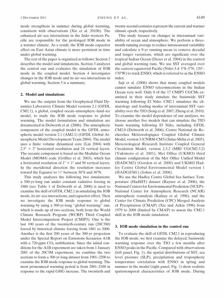
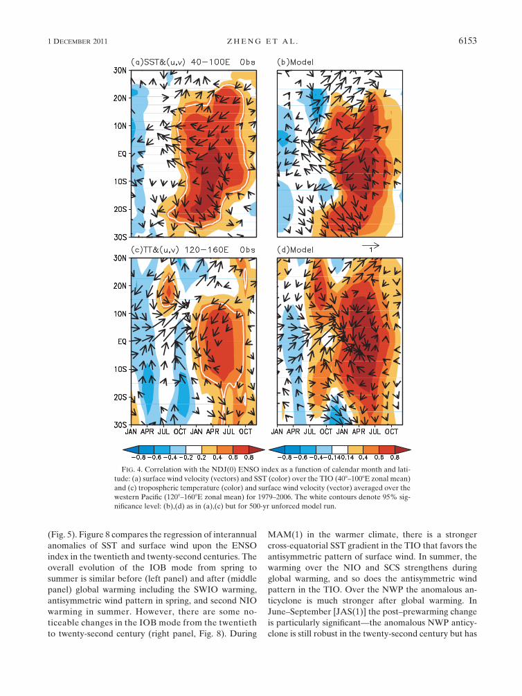
FIG. 1. Correlation with the NDJ(0) ENSO index of observed SST (color), SLP (contours), and surface wind

velocity (vectors) during (a) MAM(1) and (c) JJA(1). (b),(d) As in (a),(c) but for tropospheric temperature (contour)

and rainfall (gray shade . 0.4 and white contours at intervals of 0.1) in observations. The right-hand panels are for the

GFDL CM2.1 control run.


mode strengthens in summer during global warming,

consistent with observations (Xie et al. 2010b). The

enhanced air–sea interactions in the Indo–western Pa-

cific are responsible for the prolonged IOB mode in

a warmer climate. As a result, the IOB mode capacitor

effect on East Asian climate is more persistent in time

under global warming.

The rest of the paper is organized as follows: Section 2

describes the model and simulations. Section 3 analyzes

the control run and evaluates the simulation of IOB

mode in the coupled model. Section 4 investigates

changes in the IOB mode and its air–sea interactions in

global warming. Section 5 is a summary.

2. Model and simulations

We use the outputs from the Geophysical Fluid Dy-

namics Laboratory Climate Model versions 2.1 (GFDL

CM2.1), a global, coupled ocean–atmosphere–land–ice

model, to study the IOB mode response to global

warming. The model formulation and simulation are

documented in Delworth et al. (2006). The atmospheric

component of the coupled model is the GFDL atmo-

spheric model version 2.1 (AM2.1) (GFDL Global At-

mospheric Model Development Team 2004). The model

uses a finite volume dynamical core (Lin 2004) with

2.58 3 28 horizontal resolution and 24 vertical layers.

The oceanic component is based on the Modular Ocean

Model (MOM4) code (Griffies et al. 2003), which has

a horizontal resolution of 18 3 18 and 50 vertical layers.

In the meridional direction the resolution increases

toward the Equator to 1/38 between 308S and 308N.

This study analyzes the following two simulations:

a 500-yr-long run under constant radiative forcing in

1860 (see Table 1 of Delworth et al. 2006) is used to

examine the skill of GFDL CM2.1 in simulating the IOB

mode, its air–sea interactions, and capacitor effect. Then

we investigate the IOB mode response to global

warming by using a 300-yr-long ‘‘global warming’’ run,

which is made up of two sections, both from the World

Climate Research Program (WCRP) Third Coupled

Model Intercomparison Project (CMIP3). One is the

last 100 years of the twentieth-century run (20C3M)

forced by historical climate forcing from 1861 to 2000.

Another is the first 200 years of the 300-yr projection

under the Special Report on Emissions Scenarios A1B

with a 720-ppm CO2 stabilization. Since the initial con-

ditions for the A1B experiment are taken from 1 January

2001 of the 20C3M experiment, we combine the two

sections to form a 300-yr-long dataset from 1901–2200 to

examine the IOB mode response to global warming. The

most pronounced warming period is from 2001–2100 in

response to the rapid GHG increase. The twentieth and

twenty-second centuries represent the current and warmer

climate epoch, respectively.

This study focuses on changes in interannual vari-

ability of ocean and atmosphere. We perform a three-

month running average to reduce intraseasonal variability

and calculate a 9-yr running mean to remove decadal

and longer variations, which are significant over the

tropical Indian Ocean (Deser et al. 2004) in the control

and global warming runs. We use SST averaged over

the eastern equatorial Pacific (Nino-3.4: 58S–58N, 1208–

1708W) to track ENSO, which is referred to as the ENSO

index.

Saji et al. (2006) shows that many coupled models

cannot simulate ENSO teleconnections in the Indian

Ocean very well. Only 8 of the 17 CMIP3 CGCMs ex-

amined in their study simulate the basinwide SST

warming following El Nino. CM2.1 simulates the cli-

matology and leading modes of interannual SST vari-

ability over the TIO (Song et al. 2007; Zheng et al. 2010).

To examine the model dependence of our analyses, we

choose another five models that can simulate the TIO

basin warming following El Nino, including GFDL

CM2.0 (Delworth et al. 2006), Centre National de Re-

cherches Meteorologiques Coupled Global Climate

Model, version 3 (CNRM-CM3) (Salas-Melia et al. 2005),

Meteorological Research Institute Coupled General

Circulation Model, version 2.3.2 (MRI CGCM2.3.2)

(Yukimoto et al. 2001), Met Office (UKMO) third

climate configuration of the Met Office Unified Model

(HADCM3) (Gordon et al. 2000) and UKMO Had-

ley Centre Global Environmental Model version 1

(HADGEM1) (Johns et al. 2006).

We use the Hadley Centre Global Sea Surface Tem-

perature (HadSST) dataset (Rayner et al. 2006), the

National Centers for Environmental Prediction (NCEP)–

National Center for Atmospheric Research (NCAR)

atmospheric reanalysis (Kalnay et al. 1996), and the

Center for Climate Prediction (CPC) Merged Analysis

of Precipitation (CMAP) (Xie and Arkin 1996) from

1979 to 2008 (limited by CMAP) to assess the CM2.1

skill in the IOB mode simulation.

3. IOB mode simulation in the control run

To evaluate the skill of GFDL CM2.1 in reproducing

the IOB mode, we first examine the delayed, basinwide

warming response over the TIO a few months after

ENSO peaks in the Pacific. Compared with observations

(left panel, Fig. 1), the spatial distributions of SST, sea

level pressure (SLP), precipitation and tropospheric

temperature correlation with ENSO in spring and

summer in the model (right panel, Fig. 1) show realistic

spatiotemporal characteristics of IOB mode. During


March–May [MAM(1)], the warming is visible in the

southern TIO (Figs. 1a,e), which is due to ocean dy-

namics (Xie et al. 2002; Du et al. 2009) and heat flux

exchange (Wu et al. 2008; Wu and Yeh 2010). Both in

observations and the model (Figs. 1a,e), the antisym-

metric wind (rainfall) pattern appears over the TIO with

anomalous northeasterlies (decreased rainfall) north of

the equator and northwesterlies (increased rainfall) to

the south, accompanied with a cross-equatorial SST

gradient. The tropical tropospheric temperature anom-

alies are zonally uniform in both observations and model

during MAM(1) when El Nino signal begins its rapid

decay (Figs. 1b,f). During JJA(1) the NIO and South

China Sea warm after the summer monsoon onset, while

the antisymmetric pattern decays in the atmosphere

(Figs. 1c,g). Tropospheric temperature anomalies show

a Matsuno(1966)–Gill(1980) pattern (Figs. 1d,h). The

NWP anticyclonic circulation is present from MAM(1)

to JJA(1) in surface wind and SLP fields (Figs. 1c,g). In

MAM(1) the NWP anticyclone is maintained by local

negative SST anomalies (Wang et al. 2003). In JJA(1)

the local negative SST anomalies decay, and the remote

forcing by the TIO warming becomes the main anchor

for the NWP anticyclone (Yang et al. 2007; Xie et al.

2009). Although the model captures the main spatial

features of IO SST response to ENSO, there are some

biases as follows. The warming over the equatorial Pa-

cific is too strong and shifts westward compared with

observation, indicating the bias of simulating ENSO in

CM2.1 as is documented in Wittenberg et al. (2006). In

summer, the SST warming over the Bay of Bengal and

SCS is weaker in the model than observations.

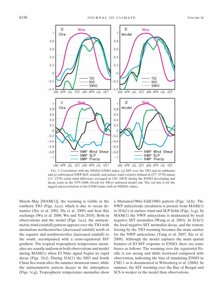
FIG. 2. Correlation with the NDJ(0) ENSO index: (a) SST over the TIO and its subbasins

and (c) subtropical NWP SLP, rainfall, and surface wind vorticity defined as (278–338N) minus

(118–158N) zonal wind difference averaged in 1208–1608E during the ENSO developing and

decay years in the 1979–2006: (b),(d) for 500-yr unforced model run. The red line is for the

lagged autocorrelation of the ENSO index with its NDJ(0) values.


The model also simulates the temporal evolution of

IOB mode realistically. Figures 2a and 2b compare the

lagged correlation with ENSO of SST averaged over the

TIO (408–1008E, 208S–208N) and its subbasins [SWIO

(508–808E, 158–58S) and NIO (408–1008E, 08–208N)] be-

tween observations and model. For 500-yr time series,

a correlation of 0.14 reaches the 99% significance level

based on t test. The model TIO warming reaches a broad

peak in MAM(1) when Nino-3.4 SST anomalies decay

rapidly. TIO SST anomalies persist through JJA(1) and

decay in August–September(1), similar to observations

(Fig. 2a). The SWIO warming, with an important con-

tribution by ocean dynamics, is maximum in March(1)

and decays in June(1). The NIO warming shows a double-

peak feature. The first warming appears during the

mature phase of El Nino while the second emerges

during JJA(1) because of the air–sea interactions within

the TIO (Izumo et al. 2008; Du et al. 2009). The NIO

warming weakens during MAM(1). This characteristic

of NIO warming is similar to observations after the mid-

1970s when ENSO is significantly stronger (Fig. 2a).

Overall, CM2.1 successfully captures the delayed TIO

warming response to El Nino.

In addition to the IOB mode, the model also simulates

the atmospheric response to El Nino over the sub-

tropical NWP. Figures 2c and 2d compare the lagged

correlation of the anomalous NWP anticyclone with

ENSO between observations and model. The anoma-

lous anticyclone emerges when El Nino reaches the

peak and persists through the summer. This result holds

whether we use a zonal wind-shear index [defined as

(27.58–32.58N) minus (108–158N) difference averaged in

1208–1608E], SLP or precipitation averaged in 12.58–

308N, 1208–1608E to represent the anticyclone. The time

evolution of the NWP anticyclone in the model is similar

to that in observations (Fig. 2c), indicating the model

skill in simulating the atmospheric response over the

subtropical NWP.

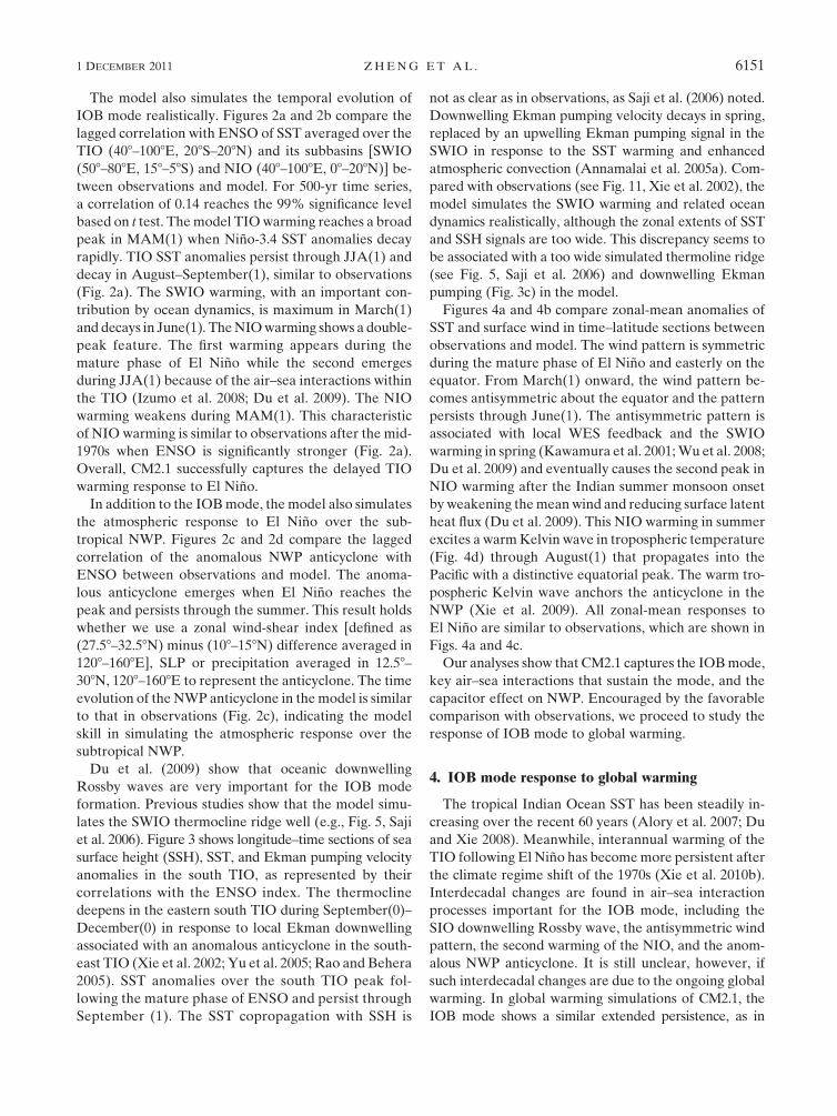
Du et al. (2009) show that oceanic downwelling

Rossby waves are very important for the IOB mode

formation. Previous studies show that the model simu-

lates the SWIO thermocline ridge well (e.g., Fig. 5, Saji

et al. 2006). Figure 3 shows longitude–time sections of sea

surface height (SSH), SST, and Ekman pumping velocity

anomalies in the south TIO, as represented by their

correlations with the ENSO index. The thermocline

deepens in the eastern south TIO during September(0)–

December(0) in response to local Ekman downwelling

associated with an anomalous anticyclone in the south-

east TIO (Xie et al. 2002; Yu et al. 2005; Rao and Behera

2005). SST anomalies over the south TIO peak fol-

lowing the mature phase of ENSO and persist through

September (1). The SST copropagation with SSH is

not as clear as in observations, as Saji et al. (2006) noted.

Downwelling Ekman pumping velocity decays in spring,

replaced by an upwelling Ekman pumping signal in the

SWIO in response to the SST warming and enhanced

atmospheric convection (Annamalai et al. 2005a). Com-

pared with observations (see Fig. 11, Xie et al. 2002), the

model simulates the SWIO warming and related ocean

dynamics realistically, although the zonal extents of SST

and SSH signals are too wide. This discrepancy seems to

be associated with a too wide simulated thermoline ridge

(see Fig. 5, Saji et al. 2006) and downwelling Ekman

pumping (Fig. 3c) in the model.

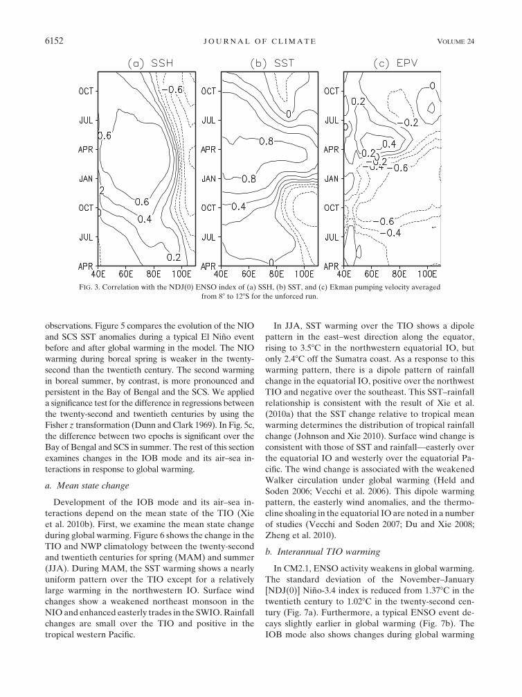
Figures 4a and 4b compare zonal-mean anomalies of

SST and surface wind in time–latitude sections between

observations and model. The wind pattern is symmetric

during the mature phase of El Nino and easterly on the

equator. From March(1) onward, the wind pattern be-

comes antisymmetric about the equator and the pattern

persists through June(1). The antisymmetric pattern is

associated with local WES feedback and the SWIO

warming in spring (Kawamura et al. 2001; Wu et al. 2008;

Du et al. 2009) and eventually causes the second peak in

NIO warming after the Indian summer monsoon onset

by weakening the mean wind and reducing surface latent

heat flux (Du et al. 2009). This NIO warming in summer

excites a warm Kelvin wave in tropospheric temperature

(Fig. 4d) through August(1) that propagates into the

Pacific with a distinctive equatorial peak. The warm tro-

pospheric Kelvin wave anchors the anticyclone in the

NWP (Xie et al. 2009). All zonal-mean responses to

El Nino are similar to observations, which are shown in

Figs. 4a and 4c.

Our analyses show that CM2.1 captures the IOB mode,

key air–sea interactions that sustain the mode, and the

capacitor effect on NWP. Encouraged by the favorable

comparison with observations, we proceed to study the

response of IOB mode to global warming.

4. IOB mode response to global warming

The tropical Indian Ocean SST has been steadily in-

creasing over the recent 60 years (Alory et al. 2007; Du

and Xie 2008). Meanwhile, interannual warming of the

TIO following El Nino has become more persistent after

the climate regime shift of the 1970s (Xie et al. 2010b).

Interdecadal changes are found in air–sea interaction

processes important for the IOB mode, including the

SIO downwelling Rossby wave, the antisymmetric wind

pattern, the second warming of the NIO, and the anom-

alous NWP anticyclone. It is still unclear, however, if

such interdecadal changes are due to the ongoing global

warming. In global warming simulations of CM2.1, the

IOB mode shows a similar extended persistence, as in


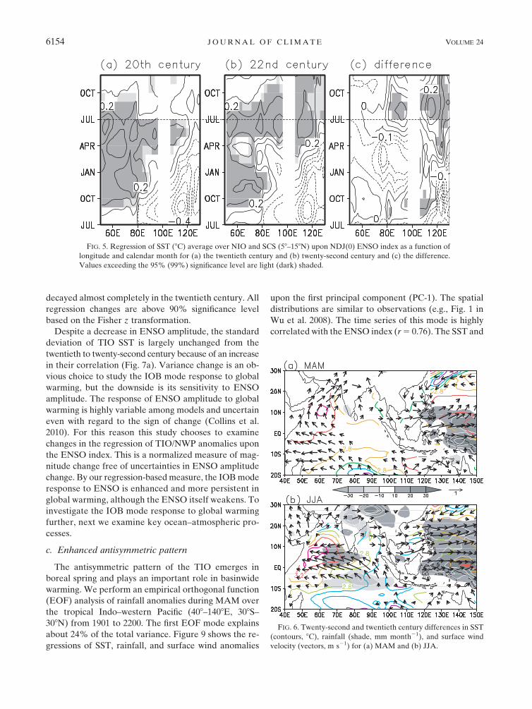
observations. Figure 5 compares the evolution of the NIO

and SCS SST anomalies during a typical El Nino event

before and after global warming in the model. The NIO

warming during boreal spring is weaker in the twenty-

second than the twentieth century. The second warming

in boreal summer, by contrast, is more pronounced and

persistent in the Bay of Bengal and the SCS. We applied

a significance test for the difference in regressions between

the twenty-second and twentieth centuries by using the

Fisher z transformation (Dunn and Clark 1969). In Fig. 5c,

the difference between two epochs is significant over the

Bay of Bengal and SCS in summer. The rest of this section

examines changes in the IOB mode and its air–sea in-

teractions in response to global warming.

a. Mean state change

Development of the IOB mode and its air–sea in-

teractions depend on the mean state of the TIO (Xie

et al. 2010b). First, we examine the mean state change

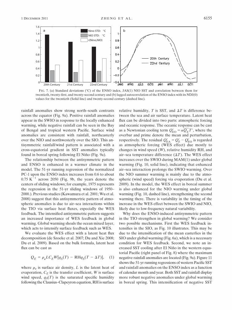
during global warming. Figure 6 shows the change in the

TIO and NWP climatology between the twenty-second

and twentieth centuries for spring (MAM) and summer

(JJA). During MAM, the SST warming shows a nearly

uniform pattern over the TIO except for a relatively

large warming in the northwestern IO. Surface wind

changes show a weakened northeast monsoon in the

NIO and enhanced easterly trades in the SWIO. Rainfall

changes are small over the TIO and positive in the

tropical western Pacific.

In JJA, SST warming over the TIO shows a dipole

pattern in the east–west direction along the equator,

rising to 3.58C in the northwestern equatorial IO, but

only 2.48C off the Sumatra coast. As a response to this

warming pattern, there is a dipole pattern of rainfall

change in the equatorial IO, positive over the northwest

TIO and negative over the southeast. This SST–rainfall

relationship is consistent with the result of Xie et al.

(2010a) that the SST change relative to tropical mean

warming determines the distribution of tropical rainfall

change (Johnson and Xie 2010). Surface wind change is

consistent with those of SST and rainfall—easterly over

the equatorial IO and westerly over the equatorial Pa-

cific. The wind change is associated with the weakened

Walker circulation under global warming (Held and

Soden 2006; Vecchi et al. 2006). This dipole warming

pattern, the easterly wind anomalies, and the thermo-

cline shoaling in the equatorial IO are noted in a number

of studies (Vecchi and Soden 2007; Du and Xie 2008;

Zheng et al. 2010).

b. Interannual TIO warming

In CM2.1, ENSO activity weakens in global warming.

The standard deviation of the November–January

[NDJ(0)] Nino-3.4 index is reduced from 1.378C in the

twentieth century to 1.028C in the twenty-second cen-

tury (Fig. 7a). Furthermore, a typical ENSO event de-

cays slightly earlier in global warming (Fig. 7b). The

IOB mode also shows changes during global warming

FIG. 3. Correlation with the NDJ(0) ENSO index of (a) SSH, (b) SST, and (c) Ekman pumping velocity averaged

from 88 to 128S for the unforced run.


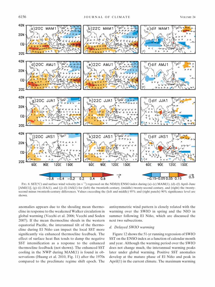
(Fig. 5). Figure 8 compares the regression of interannual

anomalies of SST and surface wind upon the ENSO

index in the twentieth and twenty-second centuries. The

overall evolution of the IOB mode from spring to

summer is similar before (left panel) and after (middle

panel) global warming including the SWIO warming,

antisymmetric wind pattern in spring, and second NIO

warming in summer. However, there are some no-

ticeable changes in the IOB mode from the twentieth

to twenty-second century (right panel, Fig. 8). During

MAM(1) in the warmer climate, there is a stronger

cross-equatorial SST gradient in the TIO that favors the

antisymmetric pattern of surface wind. In summer, the

warming over the NIO and SCS strengthens during

global warming, and so does the antisymmetric wind

pattern in the TIO. Over the NWP the anomalous an-

ticyclone is much stronger after global warming. In

June–September [JAS(1)] the post–prewarming change

is particularly significant—the anomalous NWP anticy-

clone is still robust in the twenty-second century but has

FIG. 4. Correlation with the NDJ(0) ENSO index as a function of calendar month and lati-

tude: (a) surface wind velocity (vectors) and SST (color) over the TIO (408–1008E zonal mean)

and (c) tropospheric temperature (color) and surface wind velocity (vector) averaged over the

western Pacific (1208–1608E zonal mean) for 1979–2006. The white contours denote 95% sig-

nificance level: (b),(d) as in (a),(c) but for 500-yr unforced model run.


decayed almost completely in the twentieth century. All

regression changes are above 90% significance level

based on the Fisher z transformation.

Despite a decrease in ENSO amplitude, the standard

deviation of TIO SST is largely unchanged from the

twentieth to twenty-second century because of an increase

in their correlation (Fig. 7a). Variance change is an ob-

vious choice to study the IOB mode response to global

warming, but the downside is its sensitivity to ENSO

amplitude. The response of ENSO amplitude to global

warming is highly variable among models and uncertain

even with regard to the sign of change (Collins et al.

2010). For this reason this study chooses to examine

changes in the regression of TIO/NWP anomalies upon

the ENSO index. This is a normalized measure of mag-

nitude change free of uncertainties in ENSO amplitude

change. By our regression-based measure, the IOB mode

response to ENSO is enhanced and more persistent in

global warming, although the ENSO itself weakens. To

investigate the IOB mode response to global warming

further, next we examine key ocean–atmospheric pro-

cesses.

c. Enhanced antisymmetric pattern

The antisymmetric pattern of the TIO emerges in

boreal spring and plays an important role in basinwide

warming. We perform an empirical orthogonal function

(EOF) analysis of rainfall anomalies during MAM over

the tropical Indo–western Pacific (408–1408E, 308S–

308N) from 1901 to 2200. The first EOF mode explains

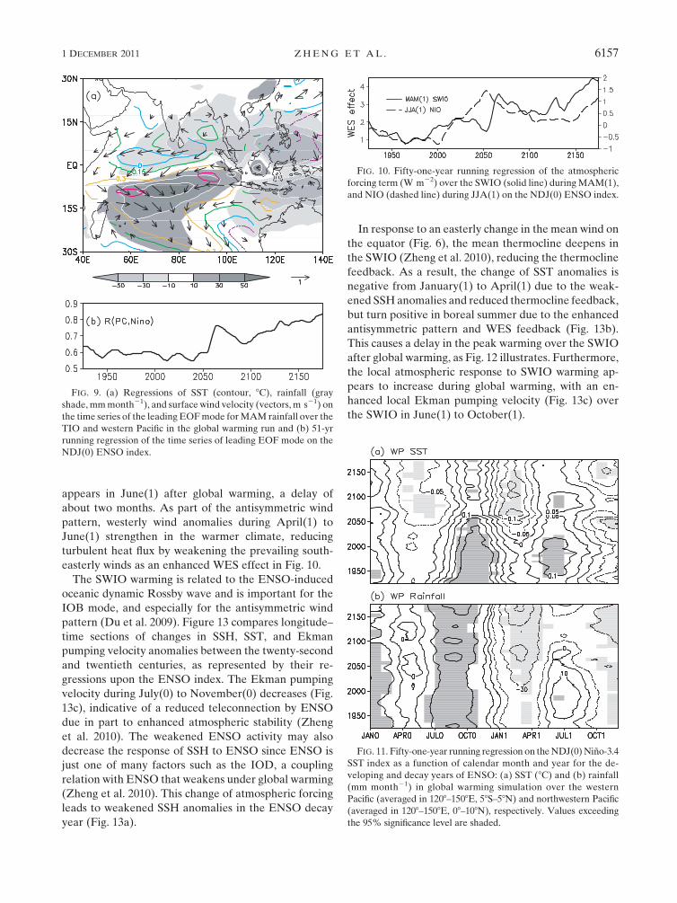
about 24% of the total variance. Figure 9 shows the re-

gressions of SST, rainfall, and surface wind anomalies

upon the first principal component (PC-1). The spatial

distributions are similar to observations (e.g., Fig. 1 in

Wu et al. 2008). The time series of this mode is highly

correlated with the ENSO index (r 5 0.76). The SST and

FIG. 5. Regression of SST (8C) average over NIO and SCS (58–158N) upon NDJ(0) ENSO index as a function of

longitude and calendar month for (a) the twentieth century and (b) twenty-second century and (c) the difference.

Values exceeding the 95% (99%) significance level are light (dark) shaded.

FIG. 6. Twenty-second and twentieth century differences in SST

(contours, 8C), rainfall (shade, mm month21), and surface wind

velocity (vectors, m s21) for (a) MAM and (b) JJA.


rainfall anomalies show strong north–south contrasts

across the equator (Fig. 9a). Positive rainfall anomalies

appear in the SWIO in response to the locally enhanced

warming, while negative rainfall can be seen in the Bay

of Bengal and tropical western Pacific. Surface wind

anomalies are consistent with rainfall, northeasterly

over the NIO and northwesterly over the SIO. This an-

tisymmetric rainfall/wind pattern is associated with a

cross-equatorial gradient in SST anomalies typically

found in boreal spring following El Nino (Fig. 9a).

The relationship between the antisymmetric pattern

and ENSO is enhanced in a warmer climate in the

model. The 51-yr running regression of the normalized

PC-1 upon the ENSO index increases from 0.6 to about

0.75 K21 across 2050 (Fig. 9b, the years denote the

centers of sliding windows; for example, 1975 represents

the regression in the 51-yr sliding windows of 1950–

2000.). Previous studies (Kawamura et al. 2001; Wu et al.

2008) suggest that this antisymmertric pattern of atmo-

spheric anomalies is due to air–sea interactions within

the TIO via surface heat fluxes, especially the WES

feedback. The intensified antisymmetric pattern suggests

an increased importance of WES feedback in global

warming. Global warming shoals the ocean mixed layer,

which acts to intensify surface feedback such as WES.

We evaluate the WES effect with a latent heat flux

decomposition (de Szoeke et al. 2007; Du and Xie 2008;

Du et al. 2009). Based on the bulk formula, latent heat

flux can be cast as

QE 5 raLCEW[qS(T) 2 RHqS(T 2 DT)], (1)

where ra is surface air density, L is the latent heat of

evaporation, CE is the transfer coefficient, W is surface

wind speed, qS(T) is the saturated specific humidity

following the Clausius–Clapeyron equation, RH is surface

relative humidity, T is SST, and DT is difference be-

tween the sea and air surface temperature. Latent heat

flux can be divided into two parts: atmospheric forcing

and oceanic response. The oceanic response can be cast

as a Newtonian cooling term Q9EO 5 aQET9, where the

overbar and prime denote the mean and perturbation,

respectively. The residual Q9EA 5 Q9E 2 Q9EO is regarded

as atmospheric forcing (WES effect) due mostly to

changes in wind speed (W), relative humidity RH, and

air–sea temperature difference (DT ). The WES effect

increases over the SWIO during MAM(1) under global

warming (Fig. 10, solid line), indicating that enhanced

air–sea interaction prolongs the SWIO warming. Over

the NIO summer warming is mainly due to the atmo-

spheric (wind speed) forcing via evaporation (Du et al.

2009). In the model, the WES effect in boreal summer

is also enhanced for the NIO warming under global

warming (Fig. 10, dashed line), strengthening the second

warming there. There is variability in the timing of the

increase in the WES effect between the SWIO and NIO,

likely due to low-frequency natural variability.

Why does the ENSO-induced antisymmetric pattern

in the TIO strengthen in global warming? We consider

two possible mechanisms. First the WES feedback in-

tensifies in the SIO, as Fig. 10 illustrates. This may be

due to the intensification of the mean easterlies in the

SIO under global warming (Fig. 6a), which is a necessary

condition for WES feedback. Second, we note an in-

creased SST cooling after El Nino in the western equa-

torial Pacific (right panel of Fig. 8) where the maximum

negative rainfall anomalies are located (Fig. 9a). Figure 11

shows the 51-yr running regressions of western Pacific SST

and rainfall anomalies on the ENSO index as a function

of calendar month and year. Both SST and rainfall display

more robust negative anomalies under global warming

in boreal spring. This intensification of negative SST

FIG. 7. (a) Standard deviations (8C) of the ENSO index, JAS(1) NIO SST and correlation between them for

twentieth, twenty-first, and twenty-second century and (b) lagged autocorrelation of the ENSO index with its NDJ(0)

values for the twentieth (Solid line) and twenty-second century (dashed line).


anomalies appears due to the shoaling mean thermo-

cline in response to the weakened Walker circulation in

global warming (Vecchi et al. 2006; Vecchi and Soden

2007). If the mean thermocline shoals in the western

equatorial Pacific, the interannual tilt of the thermo-

cline during El Nino can impact the local SST more

significantly via enhanced thermocline feedback. The

effect of surface heat flux tends to damp the negative

SST intensification as a response to the enhanced

thermocline feedback (not shown). The enhanced SST

cooling in the NWP during MAM(1) is found in ob-

servations (Huang et al. 2010, Fig. 11) after the 1970s

compared to the preclimate regime shift epoch. The

antisymmetric wind pattern is closely related with the

warming over the SWIO in spring and the NIO in

summer following El Nino, which are discussed the

next two subsections.

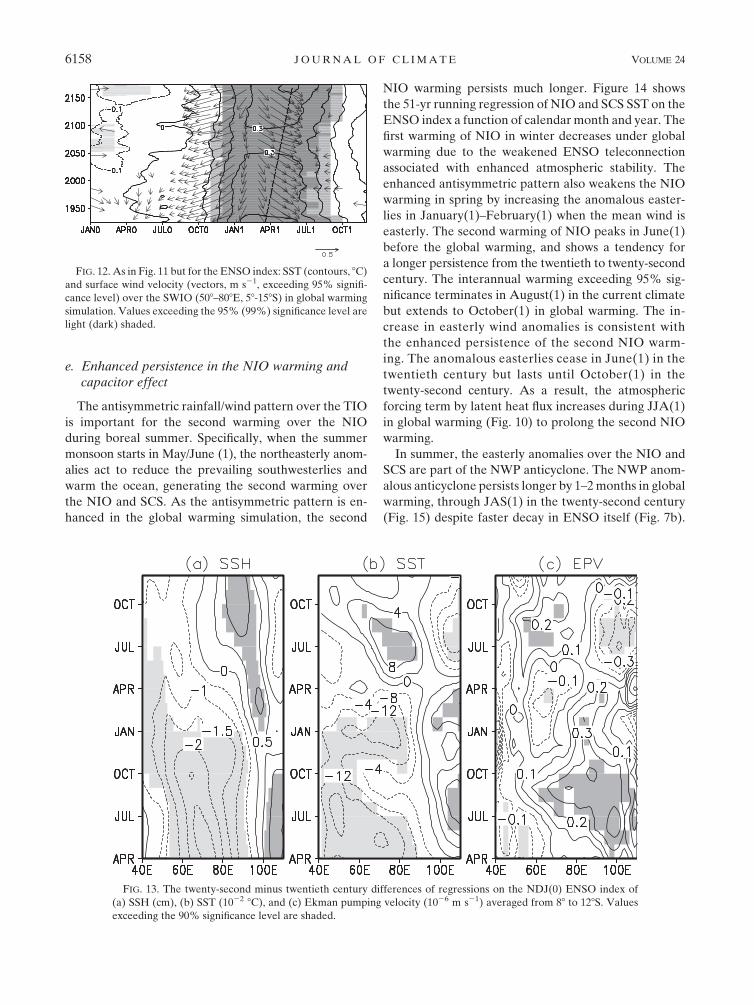
d. Delayed SWIO warming

Figure 12 shows the 51-yr running regression of SWIO

SST on the ENSO index as a function of calendar month

and year. Although the warming period over the SWIO

does not change much, the interannual warming peaks

later under global warming. Positive SST anomalies

develop at the mature phase of El Nino and peak in

April(1) in the current climate. The maximum warming

FIG. 8. SST(8C) and surface wind velocity (m s21) regressed on the NDJ(0) ENSO index during (a)–(c) MAM(1), (d)–(f) April–June

[AMJ(1)], (g)–(i) JJA(1), and ( j)–(l) JAS(1) for (left) the twentieth century, (middle) twenty-second century, and (right) the twenty-

second minus twentieth-century differences. Values exceeding the (left and middle) 95% and (right panels) 90% significance level are

shown.


appears in June(1) after global warming, a delay of

about two months. As part of the antisymmetric wind

pattern, westerly wind anomalies during April(1) to

June(1) strengthen in the warmer climate, reducing

turbulent heat flux by weakening the prevailing south-

easterly winds as an enhanced WES effect in Fig. 10.

The SWIO warming is related to the ENSO-induced

oceanic dynamic Rossby wave and is important for the

IOB mode, and especially for the antisymmetric wind

pattern (Du et al. 2009). Figure 13 compares longitude–

time sections of changes in SSH, SST, and Ekman

pumping velocity anomalies between the twenty-second

and twentieth centuries, as represented by their re-

gressions upon the ENSO index. The Ekman pumping

velocity during July(0) to November(0) decreases (Fig.

13c), indicative of a reduced teleconnection by ENSO

due in part to enhanced atmospheric stability (Zheng

et al. 2010). The weakened ENSO activity may also

decrease the response of SSH to ENSO since ENSO is

just one of many factors such as the IOD, a coupling

relation with ENSO that weakens under global warming

(Zheng et al. 2010). This change of atmospheric forcing

leads to weakened SSH anomalies in the ENSO decay

year (Fig. 13a).

In response to an easterly change in the mean wind on

the equator (Fig. 6), the mean thermocline deepens in

the SWIO (Zheng et al. 2010), reducing the thermocline

feedback. As a result, the change of SST anomalies is

negative from January(1) to April(1) due to the weak-

ened SSH anomalies and reduced thermocline feedback,

but turn positive in boreal summer due to the enhanced

antisymmetric pattern and WES feedback (Fig. 13b).

This causes a delay in the peak warming over the SWIO

after global warming, as Fig. 12 illustrates. Furthermore,

the local atmospheric response to SWIO warming ap-

pears to increase during global warming, with an en-

hanced local Ekman pumping velocity (Fig. 13c) over

the SWIO in June(1) to October(1).

FIG. 9. (a) Regressions of SST (contour, 8C), rainfall (gray

shade, mm month21), and surface wind velocity (vectors, m s21) on

the time series of the leading EOF mode for MAM rainfall over the

TIO and western Pacific in the global warming run and (b) 51-yr

running regression of the time series of leading EOF mode on the

NDJ(0) ENSO index.

FIG. 10. Fifty-one-year running regression of the atmospheric

forcing term (W m22) over the SWIO (solid line) during MAM(1),

and NIO (dashed line) during JJA(1) on the NDJ(0) ENSO index.

FIG. 11. Fifty-one-year running regression on the NDJ(0) Nino-3.4

SST index as a function of calendar month and year for the de-

veloping and decay years of ENSO: (a) SST (8C) and (b) rainfall

(mm month21) in global warming simulation over the western

Pacific (averaged in 1208–1508E, 58S–58N) and northwestern Pacific

(averaged in 1208–1508E, 08–108N), respectively. Values exceeding

the 95% significance level are shaded.


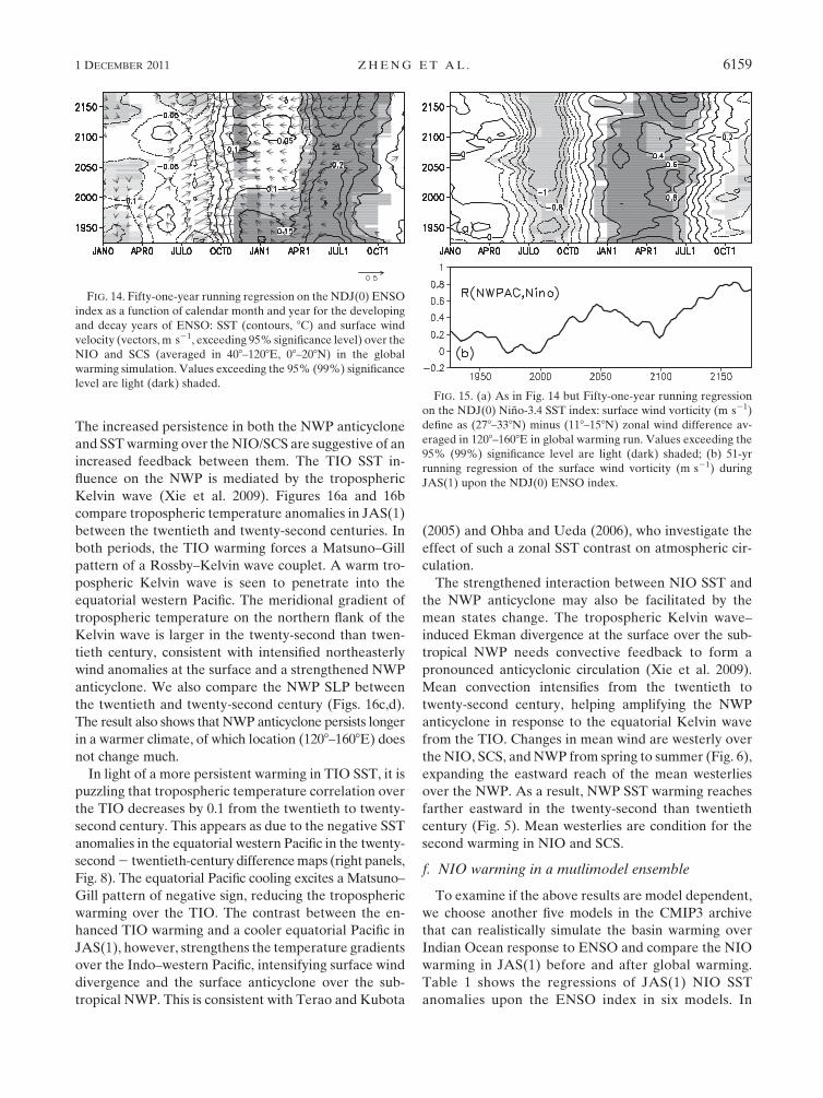
e. Enhanced persistence in the NIO warming andcapacitor effect

The antisymmetric rainfall/wind pattern over the TIO

is important for the second warming over the NIO

during boreal summer. Specifically, when the summer

monsoon starts in May/June (1), the northeasterly anom-

alies act to reduce the prevailing southwesterlies and

warm the ocean, generating the second warming over

the NIO and SCS. As the antisymmetric pattern is en-

hanced in the global warming simulation, the second

NIO warming persists much longer. Figure 14 shows

the 51-yr running regression of NIO and SCS SST on the

ENSO index a function of calendar month and year. The

first warming of NIO in winter decreases under global

warming due to the weakened ENSO teleconnection

associated with enhanced atmospheric stability. The

enhanced antisymmetric pattern also weakens the NIO

warming in spring by increasing the anomalous easter-

lies in January(1)–February(1) when the mean wind is

easterly. The second warming of NIO peaks in June(1)

before the global warming, and shows a tendency for

a longer persistence from the twentieth to twenty-second

century. The interannual warming exceeding 95% sig-

nificance terminates in August(1) in the current climate

but extends to October(1) in global warming. The in-

crease in easterly wind anomalies is consistent with

the enhanced persistence of the second NIO warm-

ing. The anomalous easterlies cease in June(1) in the

twentieth century but lasts until October(1) in the

twenty-second century. As a result, the atmospheric

forcing term by latent heat flux increases during JJA(1)

in global warming (Fig. 10) to prolong the second NIO

warming.

In summer, the easterly anomalies over the NIO and

SCS are part of the NWP anticyclone. The NWP anom-

alous anticyclone persists longer by 1–2 months in global

warming, through JAS(1) in the twenty-second century

(Fig. 15) despite faster decay in ENSO itself (Fig. 7b).

FIG. 12. As in Fig. 11 but for the ENSO index: SST (contours, 8C)

and surface wind velocity (vectors, m s21, exceeding 95% signifi-

cance level) over the SWIO (508–808E, 58-158S) in global warming

simulation. Values exceeding the 95% (99%) significance level are

light (dark) shaded.

FIG. 13. The twenty-second minus twentieth century differences of regressions on the NDJ(0) ENSO index of

(a) SSH (cm), (b) SST (1022 8C), and (c) Ekman pumping velocity (1026 m s21) averaged from 88 to 128S. Values

exceeding the 90% significance level are shaded.


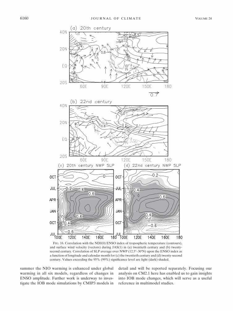
The increased persistence in both the NWP anticyclone

and SST warming over the NIO/SCS are suggestive of an

increased feedback between them. The TIO SST in-

fluence on the NWP is mediated by the tropospheric

Kelvin wave (Xie et al. 2009). Figures 16a and 16b

compare tropospheric temperature anomalies in JAS(1)

between the twentieth and twenty-second centuries. In

both periods, the TIO warming forces a Matsuno–Gill

pattern of a Rossby–Kelvin wave couplet. A warm tro-

pospheric Kelvin wave is seen to penetrate into the

equatorial western Pacific. The meridional gradient of

tropospheric temperature on the northern flank of the

Kelvin wave is larger in the twenty-second than twen-

tieth century, consistent with intensified northeasterly

wind anomalies at the surface and a strengthened NWP

anticyclone. We also compare the NWP SLP between

the twentieth and twenty-second century (Figs. 16c,d).

The result also shows that NWP anticyclone persists longer

in a warmer climate, of which location (1208–1608E) does

not change much.

In light of a more persistent warming in TIO SST, it is

puzzling that tropospheric temperature correlation over

the TIO decreases by 0.1 from the twentieth to twenty-

second century. This appears as due to the negative SST

anomalies in the equatorial western Pacific in the twenty-

second 2 twentieth-century difference maps (right panels,

Fig. 8). The equatorial Pacific cooling excites a Matsuno–

Gill pattern of negative sign, reducing the tropospheric

warming over the TIO. The contrast between the en-

hanced TIO warming and a cooler equatorial Pacific in

JAS(1), however, strengthens the temperature gradients

over the Indo–western Pacific, intensifying surface wind

divergence and the surface anticyclone over the sub-

tropical NWP. This is consistent with Terao and Kubota

(2005) and Ohba and Ueda (2006), who investigate the

effect of such a zonal SST contrast on atmospheric cir-

culation.

The strengthened interaction between NIO SST and

the NWP anticyclone may also be facilitated by the

mean states change. The tropospheric Kelvin wave–

induced Ekman divergence at the surface over the sub-

tropical NWP needs convective feedback to form a

pronounced anticyclonic circulation (Xie et al. 2009).

Mean convection intensifies from the twentieth to

twenty-second century, helping amplifying the NWP

anticyclone in response to the equatorial Kelvin wave

from the TIO. Changes in mean wind are westerly over

the NIO, SCS, and NWP from spring to summer (Fig. 6),

expanding the eastward reach of the mean westerlies

over the NWP. As a result, NWP SST warming reaches

farther eastward in the twenty-second than twentieth

century (Fig. 5). Mean westerlies are condition for the

second warming in NIO and SCS.

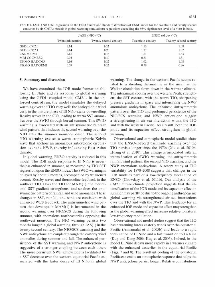
f. NIO warming in a mutlimodel ensemble

To examine if the above results are model dependent,

we choose another five models in the CMIP3 archive

that can realistically simulate the basin warming over

Indian Ocean response to ENSO and compare the NIO

warming in JAS(1) before and after global warming.

Table 1 shows the regressions of JAS(1) NIO SST

anomalies upon the ENSO index in six models. In

FIG. 14. Fifty-one-year running regression on the NDJ(0) ENSO

index as a function of calendar month and year for the developing

and decay years of ENSO: SST (contours, 8C) and surface wind

velocity (vectors, m s21, exceeding 95% significance level) over the

NIO and SCS (averaged in 408–1208E, 08–208N) in the global

warming simulation. Values exceeding the 95% (99%) significance

level are light (dark) shaded.FIG. 15. (a) As in Fig. 14 but Fifty-one-year running regression

on the NDJ(0) Nino-3.4 SST index: surface wind vorticity (m s21)

define as (278–338N) minus (118–158N) zonal wind difference av-

eraged in 1208–1608E in global warming run. Values exceeding the

95% (99%) significance level are light (dark) shaded; (b) 51-yr

running regression of the surface wind vorticity (m s21) during

JAS(1) upon the NDJ(0) ENSO index.


summer the NIO warming is enhanced under global

warming in all six models, regardless of changes in

ENSO amplitude. Further work is underway to inves-

tigate the IOB mode simulations by CMIP3 models in

detail and will be reported separately. Focusing our

analysis on CM2.1 here has enabled us to gain insights

into IOB mode changes, which will serve as a useful

reference in multimodel studies.

FIG. 16. Correlation with the NDJ(0) ENSO index of tropospheric temperature (contours),

and surface wind velocity (vectors) during JAS(1) in (a) twentieth century and (b) twenty-

second century. Correlation of SLP average over NWP (12.58–308N) upon the ENSO index as

a function of longitude and calendar month for (c) the twentieth century and (d) twenty-second

century. Values exceeding the 95% (99%) significance level are light (dark) shaded.


5. Summary and discussion

We have examined the IOB mode formation fol-

lowing El Nino and its response to global warming

using the GFDL coupled model CM2.1. In the un-

forced control run, the model simulates the delayed

warming over the TIO very well; the anticyclonic wind

curls in the mature phase of El Nino excite downwelling

Rossby waves in the SIO, leading to warm SST anoma-

lies over the SWIO through boreal summer. This SWIO

warming is associated with an antisymmetric rainfall/

wind pattern that induces the second warming over the

NIO after the summer monsoon onset. The second

NIO warming excites a warm tropospheric Kelvin

wave that anchors an anomalous anticyclonic circula-

tion over the NWP, thereby influencing East Asian

climate.

In global warming, ENSO activity is reduced in this

model. The IOB mode response to El Nino is never-

theless enhanced in summer, as measured by TIO SST

regression upon the ENSO index. The SWIO warming is

delayed by about 2 months, accompanied by weakened

oceanic Rossby waves and thermocline feedback in the

southern TIO. Over the TIO for MAM(1), the meridi-

onal SST gradient strengthens, and so does the anti-

symmetric pattern of rainfall and wind anomalies. These

changes in SST, rainfall, and wind are consistent with

enhanced WES feedback. The antisymmetric wind pat-

tern that develops in MAM(1) is instrumental in the

second warming over NIO/SCS during the following

summer, with anomalous northeasterlies opposing the

southwest monsoon. The NIO warming persists two

months longer in global warming, through JAS(1) in the

twenty-second century. The NIO/SCS warming and the

NWP anticyclone are coupled through the easterly wind

anomalies during summer and fall. The enhanced per-

sistence of the SST warming and NWP anticyclone is

suggestive of a stronger coupling between each other.

The more persistent NWP anticyclone is facilitated by

a SST decrease over the western equatorial Pacific as-

sociated with the faster decay of El Nino in global

warming. The change in the western Pacific seems re-

lated to a shoaling thermocline in the mean as the

Walker circulation slows down in the warmer climate.

The interannual cooling over the western Pacific strength-

ens the SST contrast with the warm TIO, sharpening

pressure gradients in space and intensifying the NWP

anomalous anticyclone. The enhanced antisymmetric

pattern over the TIO and prolonged persistence of the

NIO/SCS warming and NWP anticyclone suggest

a strengthening in air–sea interaction within the TIO

and with the western Pacific. As a result, both the IOB

mode and its capacitor effect strengthen in global

warming.

Observational and atmospheric model studies show

that the ENSO-induced basinwide warming over the

TIO persists longer since the 1970s (Xie et al. 2010b;

Huang et al. 2010). This change is associated with an

intensification of SWIO warming, the antisymmetric

rainfall/wind pattern, the second NIO warming, and the

NWP anomalous anticyclone. A recent study of TIO

variability for 1870–2008 suggests that changes in the

IOB mode is part of a low-frequency modulation of

ENSO (Chowdary et al. 2011b). Our analysis of the

CM2.1 future climate projection suggests that the in-

tensification of the IOB mode and its capacitor effect in

summer may partly be due to the ongoing anthropogenic

global warming via strengthened air–sea interactions

over the TIO and with the NWP. This tendency for an

enhanced IOB mode and capacitor effect may strengthen

as the global warming effect increases relative to natural

low-frequency modulation.

Observational and model studies suggest that the TIO

basin warming forces easterly winds over the equatorial

Pacific (Annamalai et al. 2005b) and leads to a rapid

termination of El Nino and a fast transition to La Nina

(Kug and Kang 2006; Kug et al. 2006). Indeed, in the

model El Nino decays more rapidly in a warmer climate

with the enhanced easterlies in the equatorial Pacific

(Figs. 7 and 8). The resultant cooling of the equatorial

Pacific can excite an atmospheric response that helps the

NWP anticyclone persist longer. Relative contributions

TABLE 1. JAS(1) NIO SST regression on the ENSO index and standard deviations of ENSO index for the twentieth and twenty-second

centuries by six CMIP3 models in global warming simulations: regressions exceeding the 95% significance level of a t test in bold.

JAS(1) NIO (8C) ENSO std dev (8C)

Twentieth century Twenty-second century Twentieth century Twenty-second century

GFDL CM2.0 0.14 0.17 1.13 1.08

GFDL CM2.1 0.14 0.20 1.37 1.02

CNRM-CM3 0.15 0.16 1.81 1.63

MRI CGCM2.3.2 0.04 0.10 0.81 1.31

UKMO HADCM3 0.16 0.17 1.02 1.08

UKMO HADGEM1 0.09 0.15 0.58 0.86


from Indian Ocean and Pacific SST anomalies to the

increased persistence of the NWP anticyclone need to

be investigated in future studies.

Acknowledgments. We would like to acknowledge

useful comments from anonymous reviewers. We wish

to thank Drs. N. C. Johnson and J. S. Chowdary for

helpful discussions. This work is supported by the Nat-

ural Science Foundation of China (40830106, 41106010,

40921004), the National Basic Research Program of China

(2012CB955603), the Fundamental Research Funds for

Central Universities of the Ministry of Education of China

(201113026), the 111 Project (B07036), the Changjiang

and Qianren Programs, the U.S. National Science Foun-

dation, and the Japan Agency for Marine-Earth Science

and Technology.

REFERENCES

Abram, N. J., M. K. Gagan, J. E. Cole, W. S. Hantoro, and

M. Mudeless, 2008: Recent intensification of tropical climate

variability in the Indian Ocean. Nat. Geosci., 1, 849–853.

Alexander, M. A., I. Blade, M. Newman, J. R. Lanzante, N.-C. Lau,

and J. D. Scott, 2002: The atmospheric bridge: The influence of

ENSO teleconnections on air–sea interaction over the global

oceans. J. Climate, 15, 2205–2231.

Alory, G., S. Wijffels, and G. Meyers, 2007: Observed temperature

trends in the Indian Ocean over 1960-1999 and associated

mechanisms. Geophys. Res. Lett., 34, L02606, doi:10.1029/

2006GL028044.

An, S.-I., J.-S. Kug, Y.-G. Ham, and I.-S. Kang, 2008: Successive

modulation of ENSO to the future greenhouse warming.

J. Climate, 21, 3–21.

Annamalai, H., P. Liu, and S.-P. Xie, 2005a: Southwest Indian

Ocean SST variability: Its local effect and remote influence on

Asian monsoons. J. Climate, 18, 4150–4167.

——, S.-P. Xie, J.-P. McCreary, and R. Murtugudde, 2005b: Impact

of Indian Ocean sea surface temperature on developing

El Nino. J. Climate, 18, 302–319.

Cai, W., A. Sullivan, and T. Cowan, 2009: Climate change con-

tributes to more frequent consecutive positive Indian Ocean

Dipole events. Geophys. Res. Lett., 36, L23704, doi:10.1029/

2009GL040163.

Capotondi, A., A. Wittenberg, and S. Masina, 2006: Spatial and

temporal structure of tropical Pacific interannual variability

in 20th century coupled simulations. Ocean Modell., 15,

274–298.

Chiang, J. C. H., and A. H. Sobel, 2002: Tropical tropospheric

temperature variations caused by ENSO and their in-

fluence on the remote tropical climate. J. Climate, 15, 2616–

2631.

——, and B. R. Lintner, 2005: Mechanisms of remote tropical

surface warming during El Nino. J. Climate, 18, 4130–4149.

Chowdary, J. S., S.-P. Xie, J.-J. Luo, J. Hafner, S. Behera,

Y. Masumoto, and T. Yamagata, 2011a: Predictability of

Northwest Pacific climate during summer and the role of the

tropical Indian Ocean. Climate Dyn., 36, 607–621, doi:10.1007/

s00382-009-0686-5.

——, ——, H. Tokinaga, Y. Okumura, H. Kubota, N. Johnson, and

X.-T. Zheng, 2011b: Inter-decadal variations in ENSO tele-

connection to the Indo-western Pacific for 1870–2007. J. Cli-

mate, in press.

Collins, M., 2005: El Nino- or La Nina-like climate change? Climate

Dyn., 24, 89–104.

——, and Coauthors, 2010: The impact of global warming on

the tropical Pacific Ocean and El Nino. Nat. Geosci., 3,

391–397.

Delworth, T. L., and Coauthors, 2006: GFDL’s CM2 global cou-

pled climate models. Part I: Formulation and simulation

characteristics. J. Climate, 19, 643–674.

Deser, C., A. S. Phillips, and J. W. Hurrell, 2004: Pacific inter-

decadal climate variability: Linkages between the tropics and

the North Pacific during boreal winter since 1900. J. Climate,

17, 3109–3124.

——, M. A. Alexander, S.-P. Xie, and A. S. Phillips, 2010: Sea

surface temperature variability: Patterns and mechanisms.

Ann. Rev. Marine Sci., 2, 115–143, doi:10.1146/annurev-

marine-120408-151453.

de Szoeke, S. P., S.-P. Xie, T. Miyama, K. J. Richards, and R. J. O.

Small, 2007: What maintains the SST front north of the equa-

torial cold tongue? J. Climate, 20, 2500–2514.

Du, Y., and S.-P. Xie, 2008: Role of atmospheric adjustments in the

tropical Indian Ocean warming during the 20th century in

climate models. Geophys. Res. Lett., 35, L08712, doi:10.1029/

2008GL033631.

——, L. Yang, and S.-P. Xie, 2011: Tropical Indian Ocean influence

on Northwest Pacific tropical cyclones in summer following

strong El Nino. J. Climate, 24, 315–322.

——, S.-P. Xie, G. Huang, and K. Hu, 2009: Role of air–sea in-

teraction in the long persistence of El Nino–induced North

Indian Ocean warming. J. Climate, 22, 2023–2038.

Dunn, O. J., and V. A. Clark, 1969: Correlation coefficients

measured on the same individuals. J. Amer. Stat. Assoc., 64,

366–377.

Fedorov, A. V., and S. G. Philander, 2000: Is El Nino changing?

Science, 288, 1997–2002.

GFDL Global Atmospheric Model Development Team, 2004: The

new GFDL global atmosphere and land model AM2-LM2:

Evaluation with prescribed SST simulations. J. Climate, 17,

4641–4673.

Gill, A. E., 1980: Some simple solutions for heat-induced tropical

circulation. Quart. J. Roy. Meteor. Soc., 106, 447–462.

Gordon, C., C. Cooper, C. A. Senior, H. T. Banks, J. M. Gregory,

T. C. Johns, J. F. B. Mitchell, and R. A. Wood, 2000: The

simulation of SST, sea ice extents and ocean heat transports in

a version of the Hadley Centre coupled model without flux

adjustments. Climate Dyn., 16, 147–168.

Griffies, S., M. J. Harrison, R. C. Pacanowski, and A. Rosati,

2003: A technical guide to MOM4. NOAA/Geophysical

Fluid Dynamics Laboratory Ocean Group Tech. Rep. 5,

295 pp.

Guilyardi, E., A. Wittenberg, A. Fedorov, M. Collins, C. Wang,

A. Capotondi, G. J. van Oldenborgh, and T. Stockdele, 2009:

Understanding El Nino in ocean–atmosphere general circu-

lation models: Progress and challenges. Bull. Amer. Meteor.

Soc., 90, 325–340.

Han, W., and Coauthors, 2010: Patterns of Indian Ocean sea level

change in a warming climate. Nat. Geosci., 3, 546–550.

Held, I. M., and B. J. Soden, 2006: Robust responses of the

hydrological cycle to global warming. J. Climate, 19, 5686–

5699.


Huang, B. H., and J. L. Kinter, 2002: Interannual variability in the

tropical Indian Ocean. J. Geophys. Res., 107, 3319, doi:10.1029/

2001JC001278.

Huang, G., K. Hu, and S.-P. Xie, 2010: Strengthening of tropical

Indian Ocean teleconnection to the Northwest Pacific since

the mid-1970s: An atmospheric GCM study. J. Climate, 23,

5294–5304.

Izumo, T., C. B. Montegut, J.-J. Luo, S. K. Behera, S. Masson, and

T. Yamagata, 2008: The role of the western Arabian Sea up-

welling in Indian monsoon rainfall variability. J. Climate, 21,

5603–5623.

Johns, T. C., and Coauthors, 2006: The new Hadley Centre climate

model HadGEM1: Evaluation of coupled simulations. J. Cli-

mate, 19, 1327–1353.

Johnson, N. C., and S.-P. Xie, 2010: Changes in the sea surface

temperature threshold for tropical convection. Nat. Geosci., 3,

842–845.

Kalnay, E., and Coauthors, 1996: The NCEP/NCAR 40-Year Re-

analysis Project. Bull. Amer. Meteor. Soc., 77, 437–471.

Kawamura, R., T. Matsumura, and S. Iizuka, 2001: Role of equa-

torially asymmetric sea surface temperature anomalies in the

Indian Ocean in the Asian summer monsoon and El Nino–

Southern Oscillation coupling. J. Geophys. Res., 106, 4681–

4693.

Klein, S. A., B. J. Soden, and N.-C. Lau, 1999: Remote sea surface

temperature variations during ENSO: Evidence for a tropical

atmospheric bridge. J. Climate, 12, 917–932.

Knutson, T. R., S. Manabe, and D. Gu, 1997: Simulated ENSO in

a global coupled ocean–atmosphere model: Multidecadal

amplitude modulation and CO2 sensitivity. J. Climate, 10, 138–

161.

Kug, J.-S., and I.-S. Kang, 2006: Interactive feedback between

ENSO and the Indian Ocean. J. Climate, 19, 1784–1801.

——, B. P. Kirtman, and I.-S. Kang, 2006: Interactive feedback

between ENSO and the Indian Ocean in an interactive en-

semble coupled model. J. Climate, 19, 6371–6381.

Lau, N.-C., and M. J. Nath, 2003: Atmosphere–ocean variations in

the Indo-Pacific sector during ENSO episodes. J. Climate, 16,

3–20.

Li, S. L., J. Lu, G. Huang, and K. M. Hu, 2008: Tropical Indian

Ocean basin warming and East Asian summer monsoon: A

multiple AGCM study. J. Climate, 21, 6080–6088.

Lin, S.-J., 2004: A ‘‘vertically Lagrangian’’ finite-volume dy-

namical core for global models. Mon. Wea. Rev., 132, 2293–

2307.

Masumoto, Y., and G. Meyers, 1998: Forced Rossby waves in the

southern tropical Indian Ocean. J. Geophys. Res., 103, 27 589–

27 602.

Matsuno, T., 1966: Quasi-geostrophic motions in the equatorial

area. J. Meteor. Soc. Japan, 44, 25–43.

Meehl, G. A., G. W. Branstator, and W. M. Washington, 1993:

Tropical Pacific interannual variability and CO2 climate

change. J. Climate, 6, 42–63.

Ohba, M., and H. Ueda, 2006: A role of zonal gradient of SST

between the Indian Ocean and the western Pacific in lo-

calized convection around the Philippines. SOLA, 2, 176–

179.

Rao, S. A., and S. K. Behera, 2005: Subsurface influence on SST in

the tropical Indian Ocean: Structure and interannual vari-

ability. Dyn. Atmos. Oceans, 39, 103–125.

Rayner, N. A., P. Brohan, D. E. Parker, C. K. Folland, J. J. Kennedy,

M. Vanicek, T. Ansell, and S. F. B. Tett, 2006: Improved

analyses of changes and uncertainties in surface temperature

measured in situ since the mid-nineteenth century: The

HadSST2 dataset. J. Climate, 19, 446–469.

Saji, N. H., S.-P. Xie, and T. Yamagata, 2006: Tropical Indian

Ocean variability in the IPCC 20th-century climate simula-

tions. J. Climate, 19, 4397–4417.

Salas-Melia, D., and Coauthors, 2005: Description and validation of

the CNRM-CM3 global coupled model, CNRM Working Note

103, 36 pp.

Schott, F. A., S.-P. Xie, and J. P. McCreary, 2009: Indian Ocean

circulation and climate variability. Rev. Geophys., 47,

RG1002, doi:10.1029/2007RG000245.

Song, Q. N., G. A. Vecchi, and A. Rosati, 2007: Indian Ocean

variability in the GFDL CM2 coupled climate model. J. Cli-

mate, 20, 2895–2916.

Terao, T., and T. Kubota, 2005: East–west SST contrast over the

tropical oceans and the post El Nino western North Pacific

summer monsoon. Geophys. Res. Lett., 32, L15706, doi:10.1029/

2005GL023010.

Timmermann, A., J. Oberhuber, A. Bacher, M. Esch, M. Latif, and

E. Roeckner, 1999: Increased El Nino frequency in a climate

model forced by future greenhouse warming. Nature, 398,

694–697.

van Oldenborgh, G. J., S. Philip, and M. Collins, 2005: El Nino

in a changing climate: A multi-model study. Ocean Sci., 1,

81–85.

Vecchi, G. A., and B. J. Soden, 2007: Global warming and the

weakening of the tropical circulation. J. Climate, 20, 4316–4340.

——, ——, A. T. Wittenberg, I. M. Held, A. Leetmaa, and

M. J. Harrison, 2006: Weakening of tropical Pacific atmo-

spheric circulation due to anthropogenic forcing. Nature,

441, 73–76.

Wang, B., R. Wu, and T. Li, 2003: Atmosphere–warm ocean in-

teraction and its impact on Asian–Australian monsoon vari-

ability. J. Climate, 16, 1195–1211.

Wittenberg, A. T., 2009: Are historical records sufficient to con-

strain ENSO simulations? Geophys. Res. Lett., 36, L12702,

doi:10.1029/2009GL038710.

——, A. Rosati, N.-C. Lau, and J. J. Ploshay, 2006: GFDL’s CM2

global coupled climate models. Part III: Tropical Pacific cli-

mate and ENSO. J. Climate, 19, 698–722.

Wu, R., and S.-W. Yeh, 2010: A further study of the tropical Indian

Ocean asymmetric mode in boreal spring. J. Geophys. Res.,

115, D08101, doi:10.1029/2009JD012999.

——, B. P. Kirtman, and V. Krishnamurthy, 2008: An asym-

metric mode of tropical Indian Ocean rainfall variability in

boreal spring. J. Geophys. Res., 113, D05104, doi:10.1029/

2007JD009316.

Xie, P., and P. A. Arkin, 1996: Analyses of global monthly pre-

cipitation using gauge observations, satellite estimates, and

numerical model predictions. J. Climate, 9, 840–858.

Xie, S.-P., and S. G. H. Philander, 1994: A coupled ocean-

atmosphere model of relevance to the ITCZ in the eastern

Pacific. Tellus, 46A, 340–350.

——, H. Annamalai, F. A. Schott, and J. P. McCreary, 2002:

Structure and mechanisms of South Indian Ocean climate

variability. J. Climate, 15, 864–878.

——, K. Hu, J. Hafner, H. Tokinaga, Y. Du, G. Huang, and

T. Sampe, 2009: Indian Ocean capacitor effect on Indo-western

Pacific climate during the summer following El Nino. J. Climate,

22, 730–747.

——, C. Deser, G. A. Vecchi, J. Ma, H. Teng, and A. T. Wittenberg,

2010a: Global warming pattern formation: Sea surface tem-

perature and rainfall. J. Climate, 23, 966–986.


——, Y. Du, G. Huang, X.-T. Zheng, H. Tokinaga, K. Hu, and

Q. Liu, 2010b: Decadal shift in El Nino influences on Indo-

western Pacific and East Asian climate in the 1970s. J. Climate,

23, 3352–3368.

Yang, J., Q. Liu, S.-P. Xie, Z. Liu, and L. Wu, 2007: Impact of the

Indian Ocean SST basin mode on the Asian summer monsoon.

Geophys. Res. Lett., 34, L02708, doi:10.1029/2006GL028571.

Yu, W., B. Xiang, L. Liu, and N. Liu, 2005: Understanding the

origins of interannual thermocline variations in the tropical

Indian Ocean. Geophys. Res. Lett., 32, L24706, doi:10.1029/

2005GL024327.

Yukimoto, S., and Coauthors, 2001: The New Meteorological

Research Institute coupled GCM (MRI–CGCM2)—

Model climate and variability. Pap. Meteor. Geophys., 51,

47–88.

Yulaeva, E., and J. M. Wallace, 1994: The signature of ENSO in

global temperature and precipitation fields derived from

the microwave sounding unit. J. Climate, 7, 1719–1736.

Zheng, X.-T., S.-P. Xie, G. A. Vecchi, Q. Liu, and J. Hafner, 2010:

Indian Ocean dipole response to global warming: Analysis of

ocean–atmospheric feedbacks in a coupled model. J. Climate,

23, 1240–1253.


Documents

Response of the Indian Ocean Basin Mode and Its …iprc.soest.hawaii.edu/users/xie/iob-change-jc11.pdfResponse of the Indian Ocean Basin Mode and Its Capacitor Effect to Global Warming*