City University of New York (CUNY) City University of New York (CUNY)

CUNY Academic Works CUNY Academic Works

Dissertations, Theses, and Capstone Projects CUNY Graduate Center

2-2020

Responses of North American Birds to Recent Climate Change: Responses of North American Birds to Recent Climate Change:

Effects of Distributional Changes on Migration Distances, Effects of Distributional Changes on Migration Distances,

Community Structure and Biodiversity Patterns Community Structure and Biodiversity Patterns

Shannon R. Curley The Graduate Center, City University of New York

How does access to this work benefit you? Let us know!

More information about this work at: https://academicworks.cuny.edu/gc_etds/3633

Discover additional works at: https://academicworks.cuny.edu

This work is made publicly available by the City University of New York (CUNY). Contact: AcademicWorks@cuny.edu

Responses of North American birds to recent climate change: Effects of distributional changes on migration distances, community structure and

biodiversity patterns

by

Shannon R. Curley

A dissertation submitted to the Graduate Faculty in Biology in partial fulfillment of the requirements for the degree of Doctor of Philosophy, The City University of New York

2020

© 2020 Shannon R. Curley All Rights Reserved

ii

Responses of North American birds to recent climate change: Effects of distributional changes on migration distances, community structure and biodiversity patterns

by

Shannon R. Curley

by Author Name This manuscript has been read and accepted for the Graduate Faculty in the Biology: Ecology, Evolution and Behavior program in satisfaction of the dissertation

requirement for the degree of Doctor of Philosophy.

__________________________ ______________________________

Date Lisa L. Manne Chair of Examining Committee __________________________ ______________________________

Date Christine Li Executive Officer

Supervisory Committee:

José D. Anadón

Frank A. La Sorte

Shaibal S. Mitra

Richard R. Veit

THE CITY UNIVERSITY OF NEW YORK

iii

Abstract

Responses of North American birds to recent climate change: Effects of distributional changes on migration distances, community structure and

biodiversity patterns

by

Shannon R. Curley Advisor: Lisa L. Manne

Species distributions are becoming increasingly altered by climate change which has been

identified as one of the leading threats to biodiversity through altered community composition. I

address changes in species distributions of North American birds and how species responses affect

community assemblages, functional traits and temporal trends in biodiversity.

Chapter 1 investigates inter-seasonal differences in range shifts for 77 species of North

American migratory birds. I quantify how shifts between winter and breeding ranges have

potentially impacted migration distances. I found that winter range shifted predominantly

northward while shifts in breeding range were more variable. These disproportional shifts have

caused decreased migration distances. Species in this study tracked their historic temperatures and

precipitation conditions in winter, but only tracked precipitation during the breeding season.

Chapter 2 focuses on species-specific responses to climate during the breeding season, and how

changes in species distributions can alter community composition. I evaluate the temporal changes

of two community indices, the Community Temperature Index (CTI), which measures

contributions of “warm” or “cool” dwelling species in a community and then establish a new

index, the Community Precipitation Index (CPI), which measures relative influences

iv

contributions of “high precipitation” or “low precipitation” affiliated species. CTI and CPI

significantly increased over time, though the strength and significance of these relationships

varied at difference latitudes. Most changes were characterized by southerly species moving to

higher latitudes and concurrent decreases in “cool” and “low precipitation” species affiliated

with urban and grassland habitats. Chapter 3 builds on the results from Chapter 2 and

investigates if these community indices inform alpha (α) and beta (ß) diversity. Species richness

decreased over time at the regional scale, and varied with latitude. CTI varied inversely with

richness, while CPI showed a positive relationship. Beta diversity also changed over time, driven

by biotic homogenization at higher latitudes, and greater community dissimilarity at the lowest

latitudes.

Multi-species, inter-seasonal studies are scare in the literature. The complementary

analyses presented in this dissertation provide new insights into the macroecological responses of

North American birds to changing climate at the population and community levels. Chapter 1

demonstrates that wintering and breeding range shifts have occur independently in North

American birds and is the first study to evaluate independent range shifts using multiple species.

Chapter 2 addresses changes in community composition in response to temperature and

precipitation and show that species contribution to CTI and CPI are different among latitude bands.

Chapter 3 expands on Chapter 2 and demonstrates that temporal trends in species turnover and

nestedness have resulted in biotic homogenization between the highest latitudes of the study.

While communities become increasingly composed of southern dwelling species moving north,

we observe decreased species richness. These chapters combined offer perspective on population

and community changes that can be used in informing conservation at the macroecology scale.

v

Acknowledgments

I would like to thank my committee members, Lisa L. Manne, Richard R. Veit, José D.

Anadón, Shaibal S. Mitra and Frank A. La Sorte for the support and guidance they have given me

over the years.

This research could not have been done without the dedication of thousands of citizen-

scientists who have generously volunteered their time to the Breeding Bird Survey and Christmas

Bird Count. I would like to thank Kathy Dale of the National Audubon Society for supplying us

with the Christmas Bird Count Data.

Thank you to the City University of New York’s Doctoral Students Research Grant

Program as well as Con-Edison, and the Research Foundation of CUNY for funding. These grants

provided me the opportunity to present my research at national and international conferences and

this exposure that has helped me grow as a researcher along the way.

During my time at CUNY I have met so many amazing people. Elizabeth Dluhos, thank

you for being the most supportive friend. You always make me laugh and have gotten me through

some of the most stressful times. José Ramírez-Garofalo, you are sitting next to me as I write this,

which is fitting. You have been next to me during this entire process and I can’t thank you enough

for your support through this all, your friendship means the world to me.

I would like to thank my family, Michael and Patricia Curley and my brother Christopher,

for their enduring patience and unconditional support. To my husband, Stephen Vargas, these last

few years have been chaotic and you have taken on so much. Thank you for always sticking by

my side and for learning how to cook!

vi

Lastly, I would like to dedicate this dissertation to my father-in-law, Dr. John Vargas.

Though you may not be here with us physically, I have felt your presence every step of this journey.

Thank you for helping me find the courage and strength to always keep pushing forward. I am

forever grateful.

vii

Contents Abstract. . . . . . . . . . . . . . . . . . . . . . . . . . . . . . . . . . . . . . . . . . . . . . . . . . . . . . . . . . . . . . . . . . . . . .iv

Acknowledgments. . . . . . . . . . . . . . . . . . . . . . . . . . . . . . . . . . . . . . . . . . . . . . . . . . . . . . . . . . . . . vi

List of Figures. . . . . . . . . . . . . . . . . . . . . . . . . . . . . . . . . . . . . . . . . . . . . . . . . . . . . . . . . . . . . . . . xi

List of Tables. . . . . . . . . . . . . . . . . . . . . . . . . . . . . . . . . . . . . . . . . . . . . . . . . . . . . . . . . . . . . . . . . xi

List of Supplementary Tables. . . . . . . . . . . . . . . . . . . . . . . . . . . . . . . . . . . . . . . . . . . . . . . . . . . . xii

Introduction. . . . . . . . . . . . . . . . . . . . . . . . . . . . . . . . . . . . . . . . . . . . . . . . . . . . . . . . . . . . . . . . . . . 1

1 Differential winter and breeding range shifts: Implications for avian migration

distances. . . . . . . . . . . . . . . . . . . . . . . . . . . . . . . . . . . . . . . . . . . . . . . . . . . . . . . . . . . . . . . . . 4

1.1 Abstract. . . . . . . . . . . . . . . . . . . . . . . . . . . . . . . . . . . . . . . . . . . . . . . . . . . . . . . . . . . . . . . . . . 4

1.2 Introduction. . . . . . . . . . . . . . . . . . . . . . . . . . . . . . . . . . . . . . . . . . . . . . . . . . . . . . . . . . . . . . . 5

1.3 Methods. . . . . . . . . . . . . . . . . . . . . . . . . . . . . . . . . . . . . . . . . . . . . . . . . . . . . . . . . . . . . . . . . . 8

1.3.1 Winter and Breeding Range Survey Data. . . . . . . . . . . . . . . . . . . . . . . . . . . . . . . . . .8

1.3.2 Species Selection and Classification. . . . . . . . . . . . . . . . . . . . . . . . . . . . . . . . . . . . . 9

1.3.3 Center of abundance (COA) of Latitude and Longitude. . . . . . . . . . . . . . . . . . . . . 10

1.3.4 Direction of COA Shifts. . . . . . . . . . . . . . . . . . . . . . . . . . . . . . . . . . . . . . . . . . . . . 10

1.3.5 Temperature and Precipitation at COAs. . . . . . . . . . . . . . . . . . . . . . . . . . . . . . . . . 11

1.3.6 Migration Distance Analysis. . . . . . . . . . . . . . . . . . . . . . . . . . . . . . . . . . . . . . . . . .12

1.4 Results. . . . . . . . . . . . . . . . . . . . . . . . . . . . . . . . . . . . . . . . . . . . . . . . . . . . . . . . . . . . . . . . . . .12

1.4.1 Directional Shifts in Winter Versus Breeding Ranges. . . . . . . . . . . . . . . . . . . . . . .12

1.4.2 Latitude Shifts Between Seasons. . . . . . . . . . . . . . . . . . . . . . . . . . . . . . . . . . . . . . .13

1.4.3 Longitude Shifts Between Seasons. . . . . . . . . . . . . . . . . . . . . . . . . . . . . . . . . . . . . .13

1.4.4 Average Temperature and Precipitation Trends at COA. . . . . . . . . . . . . . . . . . . . . 13

viii

1.4.5 Impacts on Migration Distances. . . . . . . . . . . . . . . . . . . . . . . . . . . . . . . . . . . . . . . 14

1.5 Discussion. . . . . . . . . . . . . . . . . . . . . . . . . . . . . . . . . . . . . . . . . . . . . . . . . . . . . . . . . . . . . . . .15

2 Changes in community temperature & precipitation indices over time and space reveal changing characteristics of ecological communities. . . . . . . . . . . . . . . . . . . .60 2.1 Abstract. . . . . . . . . . . . . . . . . . . . . . . . . . . . . . . . . . . . . . . . . . . . . . . . . . . . . . . . . . . . . . . . . . 60

2.2 Introduction. . . . . . . . . . . . . . . . . . . . . . . . . . . . . . . . . . . . . . . . . . . . . . . . . . . . . . . . . . . . . . .61

2.3 Methods. . . . . . . . . . . . . . . . . . . . . . . . . . . . . . . . . . . . . . . . . . . . . . . . . . . . . . . . . . . . . . . . . .63

2.3.1 Breeding Bird Survey. . . . . . . . . . . . . . . . . . . . . . . . . . . . . . . . . . . . . . . . . . . . . . . .63

2.3.2 Species Selection and Classification. . . . . . . . . . . . . . . . . . . . . . . . . . . . . . . . . . . . 63

2.3.3 Species Temperature and Precipitation Indices. . . . . . . . . . . . . . . . . . . . . . . . . . . 64

2.3.4 Community Temperature and Precipitation Indices (CTI/CPI) . . . . . . . . . . . . . . . .64

2.3.5 Modeling Spatiotemporal Trends in CTI and CPI. . . . . . . . . . . . . . . . . . . . . . . . . . 65

2.3.6 Species Contribution to CTI and CPI – Jackknife. . . . . . . . . . . . . . . . . . . . . . . . . . 65

2.3.7 Species contributions to changes in community indices. . . . . . . . . . . . . . . . . . . . .65

2.4 Results. . . . . . . . . . . . . . . . . . . . . . . . . . . . . . . . . . . . . . . . . . . . . . . . . . . . . . . . . . . . . . . . . . 66

2.4.1 Temporal trends in CTI and CPI from the Global Model. . . . . . . . . . . . . . . . . . . .66

2.4.2 Species Contributions to CTI and CPI from the Jackknife Global models. . . . . . 66

2.4.3 Temporal trends in CTI and CPI from the Latitude Bands. . . . . . . . . . . . . . . . . . .67

2.4.4 Species Contributions to CTI and CPI from the Latitude Bands. . . . . . . . . . . . . . .67

2.5 Discussion. . . . . . . . . . . . . . . . . . . . . . . . . . . . . . . . . . . . . . . . . . . . . . . . . . . . . . . . . . . . . . . 68

3 Functional community indices inform species diversity and changes in avian breeding

community composition in the eastern United States. . . . . . . . . . . . . . . . . . . . . . . . . .85

3.1 Abstract. . . . . . . . . . . . . . . . . . . . . . . . . . . . . . . . . . . . . . . . . . . . . . . . . . . . . . . . . . . . . . . . . . 85

ix

3.2 Introduction. . . . . . . . . . . . . . . . . . . . . . . . . . . . . . . . . . . . . . . . . . . . . . . . . . . . . . . . . . . . . . .86

3.3 Methods. . . . . . . . . . . . . . . . . . . . . . . . . . . . . . . . . . . . . . . . . . . . . . . . . . . . . . . . . . . . . . . . . .89

3.3.1 Community Data - Breeding Bird Survey and Study Design. . . . . . . . . . . . . . . . .89

3.3.2 Species Selection and Classification. . . . . . . . . . . . . . . . . . . . . . . . . . . . . . . . . . . .89

3.3.3 Species and Community Temperature and Precipitation Indices. . . . . . . . . . . . . .90

3.3.4 α-diversity – Rarefied Species Richness. . . . . . . . . . . . . . . . . . . . . . . . . . . . . . . . . .90

3.3.5 Temporal ß-diversity – Bray-Curtis Dissimilarity between BBS Sites. . . . . . . . . . 90

3.3.6 CTI and CPI as predictors of alpha and ß-diversity. . . . . . . . . . . . . . . . . . . . . . . . .91

3.3.7 Temporal Trends in Community Dissimilarity –

Bray Curtis Dissimilarity comparison between bands. . . . . . . . . . . . . . . . . . . . . . .92

3.4 Results. . . . . . . . . . . . . . . . . . . . . . . . . . . . . . . . . . . . . . . . . . . . . . . . . . . . . . . . . . . . . . . . . . 92

3.4.1 Rarefied Species Richness at the Regional Scale. . . . . . . . . . . . . . . . . . . . . . . . . .92

3.4.2 Rarefied Species Richness at the Local Scale. . . . . . . . . . . . . . . . . . . . . . . . . . . . .92

3.4.3 Bray Curtis Dissimilarity. . . . . . . . . . . . . . . . . . . . . . . . . . . . . . . . . . . . . . . . . . . . 93

3.4.4 Temporal Trends in Community Dissimilarity –

Bray Curtis Dissimilarity comparison between bands. . . . . . . . . . . . . . . . . . . . . . .93

3.5 Discussion. . . . . . . . . . . . . . . . . . . . . . . . . . . . . . . . . . . . . . . . . . . . . . . . . . . . . . . . . . . . . . . 94

3.5.1 Temporal Changes in Species Richness at the Regional and Local Scales. . . . . . 94

3.5.2 The Relationship Between Community Indices and Species Richness. . . . . . . . . 95

3.5.3 Temporal Changes in ß-diversity at the Regional and Local Scales. . . . . . . . . . . 96

3.5.4 Biotic Homogenization. . . . . . . . . . . . . . . . . . . . . . . . . . . . . . . . . . . . . . . . . . . . . . .97

Conclusion. . . . . . . . . . . . . . . . . . . . . . . . . . . . . . . . . . . . . . . . . . . . . . . . . . . . . . . . . . . . . . . . . .104

Bibliography. . . . . . . . . . . . . . . . . . . . . . . . . . . . . . . . . . . . . . . . . . . . . . . . . . . . . . . . . . . . . . . . .107

x

List of Tables 1.1 Generalized Linear Mixed Model (GLMM) results for winter and breeding COAs. . . . . . . . . . . . . . . . . . . . . . . . . . . . . . . . . . . . . . . . . . . . . . . . . . 26 2.1 Top 20 species with a positive percent difference from the jackknife. . . . . . . . . . . . . . . . . .77 2.2 Output from the Global model where “Year” coefficient of the model. . . . . . . . . . . . . . . .78 2.3 The top 5 species with the greatest CTIPD and CPIPD by band from the jackknife models. . . . . . . . . . . . . . . . . . . . . . . . . . . . . . . . . . . . . . . . . . . . . . . . . . 79 3.1 Results of the GLMM of species richness. . . . . . . . . . . . . . . . . . . . . . . . . . . . . . . . . . . . . 102 3.2 Results of GLMMs by latitude band. . . . . . . . . . . . . . . . . . . . . . . . . . . . . . . . . . . . . . . . . .103

List of Figures 1.1 Map of study region in North America with examples

of a) unchanged b) increased and c) decreased migration distances. . . . . . . . . . . . . . . . . 21

1.2 Significant COA shifts a) wintering range and b) breeding range. . . . . . . . . . . . . . . . . . . . 22 1.3 Boxplot of winter and summer latitude shifts. . . . . . . . . . . . . . . . . . . . . . . . . . . . . . . . . . . .23 1.4 Boxplot of winter and summer longitude shifts. . . . . . . . . . . . . . . . . . . . . . . . . . . . . . . . . . 24 1.5 Inter-seasonal comparison of latitude shifts that have resulted

in changes in migration distances. . . . . . . . . . . . . . . . . . . . . . . . . . . . . . . . . . . . . . . . . . . . .25

2.1 Map of Study area of eastern United States. . . . . . . . . . . . . . . . . . . . . . . . . . . . . . . . . . . . . 73 2.2 Mean trends in CTI (top panel) and CPI (bottom panel) from 1990 – 2017. . . . . . . . . . . . 74 2.3 Mean trends in CTI from 1990-2017. . . . . . . . . . . . . . . . . . . . . . . . . . . . . . . . . . . . . . . . . . 75 2.4 Mean trends in CPI from 1990-2017. . . . . . . . . . . . . . . . . . . . . . . . . . . . . . . . . . . . . . . . . . 76 3.1 Increasing temporal trend of mean ßBRAY at the regional scale. . . . . . . . . . . . . . . . . . . . . . 99

xi

3.2 Temporal trends in Bray Curtis Dissimilarity and its components,

balanced variation and abundance gradient. . . . . . . . . . . . . . . . . . . . . . . . . . . . . . . . . . . . 100

3.3 TukeyHSD confidence intervals of band comparisons for the earlier

time period (1990-1994) to the later time period (2013-2017). . . . . . . . . . . . . . . . . . . . . .101

List of Supplementary Tables

1.1 Change in migration distance (km yr-1) for 77 species of North American birds. . . . . . . . . 27

1.2 Shifts in Winter COAs for 77 species of North American Birds. . . . . . . . . . . . . . . . . . . . . .30

1.3 Temperature Trends at Winter “Stationary” COAs. . . . . . . . . . . . . . . . . . . . . . . . . . . . . . . .33

1.4 Precipitation Trends at Winter “Stationary” COAs. . . . . . . . . . . . . . . . . . . . . . . . . . . . . . . .36

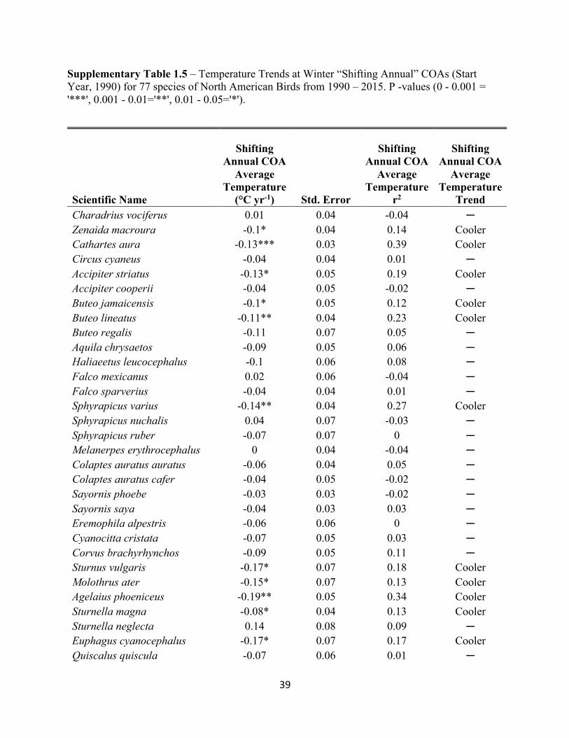
1.5 Temperature Trends at Winter “Shifting Annual” COAs. . . . . . . . . . . . . . . . . . . . . . . . . . . 39

1.6 Precipitation Trends at Winter “Shifting Annual” COAs. . . . . . . . . . . . . . . . . . . . . . . . . . . 42

1.7 Shifts in Breeding COAs for 77 species of North American Birds. . . . . . . . . . . . . . . . . . . .45

1.8 Temperature Trends at Breeding “Stationary” COAs. . . . . . . . . . . . . . . . . . . . . . . . . . . . . .48

1.9 Precipitation Trends at Breeding “Stationary” COAs. . . . . . . . . . . . . . . . . . . . . . . . . . . . . .51

1.10 Temperature Trends at Breeding “Shifting Annual” COAs. . . . . . . . . . . . . . . . . . . . . . . . . 54

1.11 Precipitation Trends at Breeding “Shifting Annual” COAs. . . . . . . . . . . . . . . . . . . . . . . . . 57

2.1 Species specific STI and SPI values and temperature and habitat associations. . . . . . . . . . . 80

xii

1

INTRODUCTION

Climate change and has been identified as one of the biggest threats to biodiversity (Bellard

et al. 2012), with consequences for species at global, regional, and local scales (Parmesan 2006).

Climate change has altered the interactions between species and their environment at individual,

population, and community levels and within ecological networks (Bellard et al. 2012).

Climate change has led to widespread shifts in species’ phenology, which have resulted in

asynchronous timing between species and seasonally abundance resources (Cayan et al. 2001,

Menzel et al. 2006, Parmesan 2006, Schwartz et al. 2006). To maintain a competitive edge, avian

species need to mitigate the effects of increased resource mismatches by adapting to changing

environmental conditions (Both & Visser 2001, Ahola et al. 2004, Saino et al. 2011). Avian

responses to changing phenology are highly variable (Both et al. 2009, Végvári et al. 2010). Some

birds arrive earlier to their breeding grounds (Van Buskirk et al. 2009), or have advanced their

breeding season (Crick & Sparks 1999). These heterogenous responses alter ecological balance by

disrupting normal patterns of inter and intraspecific competition and predator-prey dynamics

(Durant et al. 2007, Wittwer et al. 2015). This results in a reorganization of community

assemblages with potential to alter ecosystem processes (Lafferty 2009, Walther 2010, Yang &

Rudolf 2010)

In addition to changes in seasonal phenology, climate change has been identified as a driver

of change in species’ distributions (Thomas et al. 2004). In response, a wide array of taxa have

shown poleward movements in their geographic ranges (Walther et al. 2002, Parmesan & Yohe

2003, Root et al. 2003, Hickling et al. 2006, Parmesan 2006, Chen et al. 2011). Northward shifts

have been reported in avifauna of Europe and North America (Hitch & Leberg 2006, La Sorte &

Thompson 2007, Zuckerberg et al. 2009), suggesting that this ecological response is not isolated

2

to a particular region, but rather represents a much larger ecological response.

Birds have often been used as model organisms to study impacts of climate change and

ecosystem health (Both et al. 2004, Burger & Gochfeld 2004, Gregory & van Strien 2010). Birds

have high dispersal abilities and are known to track climate (Tingley et al. 2009). In addition, birds

are widely studied, and many avian monitoring programs cover over large spatial and temporal

scales. However, inter-seasonal studies of multiple species are uncommon, largely because of the

lack of suitable datasets. It is clear that independent processes in the annual life cycles of birds

should be accounted for in conservation strategies (Doswald et al. 2009, Zurell et al. 2018). For

example, migratory species—which occupy distinct wintering and breeding grounds— should be

impacted if their winter and breeding ranges are under different ecological pressures. These shifts

could impact the distance and time needed to travel between locations, thus affecting the timing of

resource availability on breeding grounds. Migration is physiologically taxing and migratory

species will need to adjust to altered phenology to avoid increasing mismatches with resources

(Saino et al. 2010).

I took advantage of two long-term, continent-wide surveys of avian abundance that occur

during the wintering and breeding seasons for North American birds; the National Audubon

Society Christmas Bird Count (CBC; National Audubon Society 2017) and the North American

Breeding Bird Survey (BBS; US Geological Survey Patuxent Wildlife Research Center 2017).

The CBC was established in 1900, and has continued annually. The CBC represents the world’s

oldest and most comprehensive dataset on avian populations (Butcher 1990). The BBS was

established in 1966 by the United States Fish and Wildlife Service and Canadian Wildlife Service

as a continent-wide network of avian survey routes to monitor avian declines resulting from the

widespread agricultural use of DDT (Peterjohn et al. 1995). Over the next few decades, routes

3

expanded into Alaska and the Northwest Territories as well as Mexico (Peterjohn et al. 1995).

Each of these surveys rely heavily on the contributions and participation of volunteer observers.

These two citizen science monitoring programs have become valuable resources for addressing

long-term impacts of climate change on avian populations.

In each chapter of this dissertation, I address patterns that occur at the population or

community level, and where applicable, provide information on individual species contributions

to overall trends and patterns. In Chapter 1, I test the hypothesis that winter and breeding

distributions are changing at the same rate. I find that they are largely shifting at different rates

(and sometimes in different directions) and I assess the impacts on migration distances. In chapter

2, I test the hypothesis that community climate indices are predictive of community functional

traits. I find that avian communities are becoming increasingly composed of species adapted to

warm and wet environments. In chapter 3, I again study community climate indices, and their

effectiveness at predicting multiple biodiversity measures. I test the hypothesis that community

climate indices are predictive of biodiversity, and find that community indices of temperature and

precipitation have significant, but opposing relationships with alpha diversity. However, I found

no relationships between the community indices and beta diversity.

4

Chapter 1

Differential winter and breeding range shifts: Implications for avian migration distances

(in press for Diversity and Distributions)

1.1 ABSTRACT

Aim: For many migratory avian species, winter and breeding habitats occur at geographically

distinct locations. Disparate magnitudes and direction of shifts in wintering and breeding locations

could lead to altered migration distances. We investigated how shifts in the center of abundance

(COA) of winter and breeding ranges have changed for 77 species of short distance migratory

birds. We addressed whether species tracked their historical average temperature and precipitation

conditions at their winter and breeding COA, using data from 1990-2015.

Location: North America

Methods: We calculated the COA for winter and breeding ranges from the National Audubon

Society’s Christmas Bird Count and the North American Breeding Bird Survey. We regressed the

annual change in distance (km) between the two annual COAs of each species as a proxy for

change in migration distance. We constructed a series of Generalized Linear Mixed Models

(GLMMs) to evaluate changes in average temperature and precipitation at the wintering and

breeding COAs.

Results: Winter shifts in COA were predominantly northward. For most species, average

temperature and precipitation that species experienced had not changed. Breeding shifts in COA

varied in direction. For breeding season COAs, average temperature warmed, but average

precipitation had not changed. Thirty-one species significantly decreased their migration distances,

5

mainly driven by northward shifts in the winter range. Ten species increased their migration

distances.

Main Conclusions: Winter and breeding range shifts in COA have not occurred at the same

magnitude and direction, and have therefore impacted distance migrated. Our results suggest that

wintering and breeding range shifts occur independently, and under different climate pressures.

1.2 INTRODUCTION

Avian migration is an annual movement across landscapes to take advantage of seasonally

variable resources (Alerstam & Lindström, 1990). It is a widely documented behavior found on all

continents and oceans (Alerstam, Hedenström, & Åkesson, 2003). The seasonal movement of

migrating individuals has long-term impacts on biodiversity and ecosystem processes (Bauer &

Hoye, 2014). Understanding how migratory patterns are changing over time is important for

conservation planning.

Anthropogenic land-use and climate change are altering species distributions (Walther et

al., 2002; Parmesan & Yohe, 2003; Sparks, Roy & Dennis, 2005; Hickling, Roy, Hill, Fox, &

Thomas, 2006; Parmesan 2006; Chen, Hill, Ohlemüller, Roy, & Thomas, 2011; Van der Hoek,

Renfrew, & Manne, 2013; Van der Hoek et al., 2015). Predicting how migratory species might

respond to landscape level changes presents additional challenges as breeding and wintering

habitats generally occur at geographically disjoint locations (Knudsen et al., 2011). The effects of

climate change are projected to be the most pronounced in the winter, and at higher latitudes (IPCC

2013). The phenomena that elicit changes in species distributions in one portion of an annual range

may not exist in another. Different portions of a migratory species’ range might experience

different conditions throughout the annual cycle; therefore, it is necessary to look at each portion

of the range independently to understand how distributions are changing throughout an annual

6

cycle. If disparate magnitudes and directions of range shifts are occurring between breeding and

wintering locations, the migratory distance between the two will likely change (Doswald et al.,

2009; Huntley et al., 2006).

Northward range shifts have been documented in birds in summer (Thomas & Lennon

1999; Hitch & Leberg 2006; Zuckerberg, Woods, & Porter, 2009) and winter (La Sorte &

Thompson 2007). However, recent literature has emphasized that species-specific movements are

more complex and variable due to the interactions between temperature, precipitation and land-

use changes (Tingley, Monahan, Beissinger, & Moritz, 2009; Lenoir et al., 2010; VanDerWal et

al., 2013). Multidirectional shifts – shifts having a latitude and longitude component – can be

evaluated by incorporating measures of central tendency of a species range. Using central tendency

measures, multidirectional shifts have been documented in North America and Europe for various

birds, trees and plant species (Ash, Givnish, & Waller, 2017; Currie & Venne, 2017; Fei et al.,

2017; Huang, Sauer, & Dubayah, 2017; Pavón‐Jordán et al., 2018).

Most knowledge of how migration patterns might be changing in birds comes from banded-

bird data. In the Netherlands, Visser, Perdeck, van Balen, & Both (2009) analyzed 72 years of

banded-bird recovery data and found half of the species experienced shortened migration

distances. They implicate climate change as the mechanism for birds wintering closer to their

breeding grounds. Potvin, Välimäki, & Lehikoinen (2016) found that winter and breeding range

shifts do not necessarily occur at equal rates, and not all species shift in the same direction,

resulting in species-specific changes in migration distance. This research also suggests flexibility

in migratory behavior, influenced by independent environmental changes occurring between

ranges.

The availability of high-quality, long-term data sets make birds good candidates to observe

7

effects of climate on species distributions. In this study, we use two long-term avian monitoring

programs, the North American Breeding Bird Survey (BBS; US Geological Survey Patuxent

Wildlife Research Center, 2015) and National Audubon’s Christmas Bird Count (CBC; National

Audubon Society, 2015). These datasets offer continental-scale quantitative data, and represent

some of the most systematic and complete sampling of any taxa. We examined changes in center

of abundance (COA) for temporally shifting breeding and winter ranges to understand how

migration direction and distance is shifting between the two and used COA movement between

seasons as a proxy for migration distance.

In this study we address four complementary hypotheses to examine how species have

shifted over time. First, we test the hypothesis that winter and breeding COAs have shifted at same

rate and direction. We expect that winter COA shifts will occur more rapidly northward than their

breeding range counterparts. Our expectations are derived from recent studies of North American

Birds which have documented northward winter range expansion (La Sorte & Thompson 2007)

but more species-specific variability of movements in the breeding season (Huang, Sauer, &

Dubayah 2017, Currie & Venne 2017). Second, we test the hypothesis that the distance between

winter and breeding COAs has not changed, therefore migration distances have been unaffected.

We expect that most species have decreased their distance between winter and breeding COAs and

have experienced shortened migration distances driven, primarily driven by northward winter

COA shifts exceeding the rates of breeding COAs (Visser et al., 2009; Potvin et al., 2016). We

further assessed two additional hypotheses of how temperature and precipitation have changed and

evaluate if species have tracked their recent historical climate conditions. We test if temperature

and precipitation have changed at the start-year (“stationary”) COA locations. A significant change

at the “stationary” COAs provide evidence that species have experienced changes in temperature

8

and precipitation from a previously occupied COA (a potential reason for species to shift away

from a location). Lastly, we test if temperature and precipitation have not changed at the locations

that species have annually shifted to (“shifting-annual”) COA locations. Our expectation is that

temporally unchanged conditions at a species “shifting annual” COA suggests that species had

moved to areas with similar historic conditions.

1.3 METHODS

1.3.1 Winter and Breeding Range Survey Data

We calculated center of abundance (COA) for winter (December-January) and breeding

ranges (May-June) for North American short-distance migratory birds from 1990 to 2015 from

CBC and BBS, respectively. Since COA calculations are sensitive to spatiotemporal bias, we

restricted our analysis to this 26-year period. This helped to standardize the spatial sampling

between our two datasets and to avoid artificial shifts in COA, which would be an artifact of the

rapid addition of survey routes prior to the years of our study.

The BBS is a network of annually sampled roadside survey routes. Surveys are conducted

during the month of June to coincide with the peak of the breeding season for many avian species.

Each route is 39.4 km long with 50 census locations spaced throughout. At each census location,

a 3-minute point count is taken, where all birds that are seen or heard within a 0.4 km radius are

recorded (US Geological Survey Patuxent Wildlife Research Center, 2015).

CBC censuses are conducted within a two-week window around December 25th. Each

census is annually surveyed in a 24.14 km diameter of a chosen center point. The center point of

the circle does not vary from year to year. Abundances of all birds seen or heard within the circle

are recorded (National Audubon Society, 2015). Effort data (in terms of party hours) can vary

9

within and across CBC circles, therefore, we standardized the overall avian abundances in each

CBC circle by the number of party hours for each count circle unit (Raynor, 1975).

To keep the network of routes relatively stationary over time, BBS routes and CBC circles

were temporally filtered to exclude all routes missing 2 or more consecutive years of sampling.

No routes south of the United States border met the filtering criterion. We eliminated areas where

both BBS and CBC surveys were sparsely sampled by only including surveys that occurred below

56.6° latitude and fell between -125 and -75° longitude (as did Currie & Venne 2017). Using these

criteria, we retained 1,326 BBS routes and 1,321 CBC circles for the analysis. To check for any

spatial bias between our datasets, we regressed the mean latitude and longitude of CBC and BBS

sampling sites over time. For CBC locations we found a 0.11 km yr-1 shift south and a 0.78 km yr-

1 shift to the west. For BBS locations we found no significant trend in latitude over time. We found

a westward rate of 1.66 km yr-1 shift for longitude. The effect of these shifts on species-specific

responses should therefore be small and unbiasing.

1.3.2 Species Selection and Classification

We followed the migratory guild classification of BBS to obtain a pool of “short-distance

migrants”: species whose migratory movements are primarily intra-continental in North America.

Neotropical migrants (species that breed in the United States and Canada but overwinter in

Mexico, Central America, South America and the Caribbean Islands) were not included in this

analysis because most wintering ranges fall outside of the CBC coverage area. We further filtered

out species with known irruptive migratory patterns —Pine Siskin (Spinus pinus), Red Crossbill

(Loxia curvirostra), Evening Grosbeak (Coccothraustes vespertinus)—and coastal species whose

COA for any year was over water —Fish Crow (Corvus ossifragus), Osprey (Pandion haliaetus),

10

Tree Swallow (Tachycineta bicolor) and White-winged dove (Zenaida asiatica). In total, 77

species of short-distance migrants met these criteria and were included in this study.

1.3.3 Center of abundance (COA) of Latitude and Longitude

For each species and range (winter and breeding), we calculated an annual COA. Each

COA is an average longitude (x) and latitude (y) calculated from abundance indices from each

location. For the winter ranges, the latitudes and longitudes in the calculation were from the center

point of each CBC circle. For breeding ranges, the latitudes and longitudes were from the starting

point of each survey route. We used the following formulas to calculate an annual COA abundance

for each species:

Weighted latitudet = Σ(latitudei,t × abundancei,t ) ÷ total abundancet

Weighted longitudet = Σ(longitudei,t × abundancei,t ) ÷ total abundancet

Where latitudei,t and longitudei,t are the latitude and longitude of an individual site i and the

corresponding abundance for year t. Total abundance is the sum of all individuals of the species

for that year across all the sites (either BBS routes or CBC circles).

Annual COAs were derived from a paired weighted latitudet and weighted longitudet:

COAt = (weighted latitudet,weighted longitudet). 1.3.4 Direction of COA Shifts

We regressed the annual latitude and longitude components of COA separately against year

for each species (degree shift yr-1). For the latitude component and the longitude component, we

identified north and south shifts by regression slopes that were significantly greater or less than 0.

Significant shifts to the northeast, southeast, southwest and northwest occurred when both the

11

latitude and longitude components had significant regression slopes (e.g. shifts of COA to the

northeast are the results of significant positive latitude and longitude slopes). We report these

results in km shift yr-1.

1.3.5 Temperature and Precipitation at COAs

We acquired seasonal temperature and precipitation variables from the CRU-TS 3.22

historical dataset (Mitchell & Jones, 2005) downloadable from the open-source software

ClimateNA. v5.21 (http://tinyurl.com/ClimateNA), based on methodology described by Wang et

al. (2016). Climate variables are gridded at a 0.5x0.5° resolution. We obtained average winter and

summer temperature (°C) and precipitation (mm) for each COA/year combination. To evaluate if

species have tracked temporal changes in average temperature and precipitation over the study

period, we produced two sets of Generalized Linear Mixed Models (GLMMs; Zuur et al., 2009).

In each of the models, average temperature and precipitation were the response variables and year

was treated as a continuous variable. We included species as a random effect in the model,

therefore allowing the y-intercepts to vary among species which helped to account for geographic

and species-specific differences in COA. In the first set of models, we used the initial winter and

breeding range COA coordinates for each species from year 1990, assumed these COAs would not

shift, and traced the average temperature and precipitation at this “stationary” COA over time. If

COAs do not shift, but climatic properties of those COAs do change, the birds experience changed

climatic parameters. In the second set of models, we obtained the average temperature and

precipitation at each annual “shifting” COA. If we detected no significant changes in temperature

and precipitation at this “shifting” COA, then the birds experienced similar climatic parameters

from year to year. We conducted this analysis to show the difference between unchanging

conditions (as if the environmental conditions of 1990 remain constant), and what we deduce the

12

birds experienced at shifting COAs. We provide the individual species regressions results in the

supplementary file.

1.3.6 Migration Distance Analysis

As a proxy for migration distance we calculated the Haversine distance (km) between

winter and breeding COA for each year and species using R package ‘geosphere’ (Hijmans,

Williams & Vennes, 2015). Haversine distance measures the shortest distance between two points

on a sphere. This was a more precise measurement for changes between COA while accounting

for the curvature of the Earth. Annual migration distance was regressed against year to test

whether the slopes were significantly different from zero for each of the species. Significant

positive or negative slopes indicate increasing and decreasing migration distance, respectively.

Non-significant slope values indicate no change in migration distance. From this analysis we

partitioned species into groups: species with a) statistically unchanged, b) increased, or c)

decreased migration distances over this time period (Figure 1.1). To evaluate average change in

migration distance over time we produced a GLMM with migration distance as the response and

year as a continuous predictor, with species as a random factor.

1.4 RESULTS

1.4.1 Directional Shifts in Winter Versus Breeding Ranges

In winter, many species (31.1%) have not changed the location of their winter COA. For

species with significantly changed COAs, the most frequently observed shift was to the north

(29.8%), followed by northeast (11.6%), northwest (10.3%), east (7.9%), south (3.8%) and

southeast (2.5%) west (2.5%). No species in this study shifted their winter COA to the southwest

(Figure 1.2a).

During the breeding season, many species (22.0%) did not significantly shift their COA.

13

When shifts in COA occurred, they were comparatively more variable in direction. The most

frequently observed shifts were to the northwest (14.2%) and southwest (12.9%), followed by

south (11.6%), north (10.3%), west (10.3%), east (7.7%), southeast (6.4%) and northeast (3.8%)

(Figure 1.2b).

1.4.2 Latitude Shifts Between Seasons

On average, species in this study shifted the latitude component of their COA northward

in winter and slightly southward during the breeding season. In winter, northward shifts occurred

at an average rate of 3.09 km yr -1. In summer, this rate was significantly lower at -0.003 km yr -1

and not significantly different from zero (t = 5.1878, df= 76, p-value= 1.811e-08, Figure 1.3). The

difference in these rates was driven by the larger number of species shifting the latitude component

of their COA southward during the breeding season (e.g. as shown in Figure 1.2b).

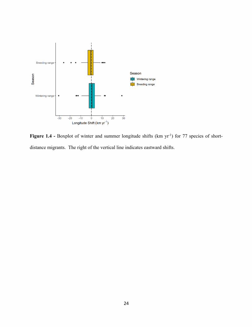
1.4.3 Longitude Shifts Between Seasons

Longitude shifts in COA occurred at the same rate in the winter and breeding seasons and

were not significantly different from zero. Winter ranges shifting slightly eastward at a rate of

0.092 km yr -1 and slightly westward in the breeding season at 1.09 km yr -1 (t = 1.436, df= 76, p-

value= 0.155, Figure 1.3). These low rates of close to 0 km yr -1 are driven by almost equal

numbers of species shifting eastward and westward within a season. In addition, these shifts

occurred at similar magnitudes within and between seasons.

1.4.4 Average Temperature and Precipitation Trends at COA

From the results of the GLMMs we found that the average winter temperature and

precipitation at the 1990 (“stationary”) COAs had significantly declined (p < 0.001) but had not

significantly changed at the shifting annual COAs for either variable (Table 1). Average summer

14

temperature had significantly increased at the stationary (p < 0.001) and shifting annual breeding

range COAs (p < 0.001). Precipitation had not significantly changed at the stationary or shifting

annual COA (Table 1).

1.4.5 Impacts on Migration Distances

Across all species, average migration distances have decreased at a rate of ~2.9 ± 0.4 km

yr-1 (p = <0.001). In this study 36 (46.8%) did not significantly change their migration distance

over the time period. In total, 41 species have changed their migration distance, and the majority

of these shifts were attributed to significant shifts in latitude, with fewer species exhibiting changes

due to shifts in longitude. We found a decrease in migration distance for 31 (40.3%) species and

increased migration distance for 10 (12.9%) species (Figure 1.4). Of the group of species who have

decreased their migration distance, 22/31 of these were driven by northward winter shifts of COA

exceeding the rate of breeding shifts of COA. Many species demonstrated decreased distances

between winter and breeding COA by a combination of southward shifts in breeding COA and

northward shifts in winter COA (Supplementary Material). For four species, Red-shouldered

Hawk (Buteo lineatus), Bald Eagle (Haliaeetus leucocephalus), Western Meadowlark (Sturnella

neglecta), and Lesser Goldfinch (Spinus psaltria), the decreased distance between winter and

breeding COA are explained by significant shifts in longitude (Figure 1.4, Supplementary

Material).

Ten species have increased their distance between their winter and breeding COA (Figure

1.4b). For 6 species, these increases were the result of breeding latitude shifts in COA exceeding

the rate of shift in the winter COA counterpart. Shifts in longitude explained the increased

migration distance for remaining 4 species; American Crow (Corvus brachyrhynchos), House

15

Finch (Haemorhous mexicanus), Fox Sparrow (Passerella iliaca) and Bewick’s Wren

(Thryomanes bewickii) (Figure 1.4, Supplementary Material).

1.5 DISCUSSION

Despite the prevalence of migratory species, literature on migratory systems is

disproportionately small (Berger 2004; Harris, Thirgood, Hopcraft, Cromsigt, & Berger, 2009).

Understanding how migratory patterns are changing under climate change is important for long-

term conservation planning and management. This study uses broad-scale spatiotemporal

abundance survey data to examine inter-seasonal shifts in COA, and how these shifts are

potentially altering migratory distances. Assessment of how migration distances are changing is

scarce in the literature, but we can speculate that these changes are occurring, and have

consequences on both individual fitness and long-term population trends for migratory birds.

Recent literature emphasizes species-specific multidirectional shifts in distributions

(VanDerWal et al., 2013; Gillings, Balmer, & Fuller, 2015; Huang et al., 2017; Currie & Venne

2017, Fei et al., 2017). Complex interactions between temperature and precipitation are driving

species-specific responses to changes in climate (Tingley et al., 2009; Tingley et al., 2012;

VanDerWal et al., 2013; Garcia et al., 2014). Birds have been shown to geographically track their

historical climatic niches (Tingley et al., 2009). While most studies focus on temporal changes

occurring within a single season, there are few comparative studies looking at species-specific

shifts between two distinct periods (but see Potvin et al., 2016; Zurell, Graham, Gallien, Thuiller,

& Zimmermann, 2018). We offer evidence that environmental variables are differentially tracked

between seasons, and that distributions throughout the annual cycle are independent. These

temporal and disjunct seasonal changes in distributions suggest flexibility of migratory behavior,

at least at the macroecological scale.

16

We found that winter movements in COA were primarily occurring in a northward

direction, with 51.9% of the species having a significant northward shift in the latitude component

of their COA. Our results are consistent with the pole-ward shifts documented in North American

birds during the winter (La Sorte & Thompson 2007) and also in Europe (Visser et al., 2009; Potvin

et al., 2016). Our reaffirmation of northward winter shifts was therefore not surprising, as birds

are known to be physiologically constrained by winter temperatures (Root 1988) and temperature-

driven northward shifts of wintering birds has been widely documented (La Sorte and Thompson

2007; Lehikoinen et al., 2013; Pavón-Jordán et al., 2018). Though our finding that winter

temperatures have declined at the stationary COA locations appears at odds with the current

warming trends that have occurred over a longer time period (United States Global Change

Research Program, 2018), cooling trends in the south and southeastern united states have been

documented since the 1950’s. This large area of declining temperatures is referred to as the U.S.

“warming hole” (Pan et al., 2004). The “warming hole” is likely the product of warming

temperatures in the Arctic and the melting of sea ice being driving southward by air currents,

creating cooler than expected temperatures in parts of the United States during the winter

(Partridge et al., 2018). Of our 77 “stationary” COAs, 45 occur east of -100°W longitude and fall

approximately within the warming hole as mapped by Partridge et al (2018). Though our cooling

trend is significant, the slope of this relationship is very small, representing a 0.26°C cooling over

the 26-year time period (Table 1).

In this study, average winter temperature and precipitation have remained consistent at the

shifting annual COA for most species. Climate conditions as a whole appear to be an important

factor for wintering locations for migratory birds (Somveille, Rodrigues, & Manica, 2015; Pérez-

Moreno, Martínez-Meyer, Soberón Mainero, & Rojas-Soto, 2016). Despite northward shifts in

17

winter COAs, we did not detect many instances where temperature was significantly changing at

these shifting annual COAs. From the resolution of our data, it appears that species are shifting

their winter COAs in a manner consistent with the pattern of climate change (Parmesan & Yohe,

2003; Chen et al., 2011).

We found that breeding season movements of COA were more variable in direction in

comparison to winter movements. Despite this variability, most species experienced warming at

their both their 1990 “stationary” and “shifting annual” COA. Average precipitation however, was

unchanged at the 1990 “stationary” and “shifting annual” COAs. Maintaining consistent annual

precipitation might be important as precipitation during the breeding season is known to limit

survivorship in birds (Sillett, Holmes, & Sherry, 2000) and is indirectly linked to food resource

availability (Carroll, Cardinale, & Nisbet, 2011).

Avian species distributions appear to be susceptible to environmental changes along

longitudinal gradients, as well as latitudinal ones. Westward shifts were common; 37.6% of the

species had significant westward longitude shifts in their breeding COA. Our results are consistent

with two recent analyses of North American birds that also found high occurrences of avian

abundances shifting west during the breeding season (Huang et al., 2017; Currie & Venne 2017).

Additionally, Fei et al., (2017) examined 86 tree species across the eastern United States and most

commonly observed westward range shifts over the course of 30 years. Sapling recruitment was

highest at the western edges of ranges, particularly for drought-resilient species with the ability to

exploit increasing moisture patterns within drier, western areas. Interaction between warming

temperature and changing precipitation patterns offers the potential to differentially impact species

via their individual tolerances, which might explain our observed variability in summer.

While significant shifts in COA were evident between seasons 46.8% of the species in this

18

study have not differentially shifted their winter and summer COAs enough to impact migration

distance. We categorize these results in 3 ways: A) neither COA has shifted in summer and winter

(7 species), B) Winter and summer COA shifts have occurred in roughly equal magnitudes and

directions (5 species), or C) direction and magnitude of a COA shift in one season is not large

enough to significantly affect migration distance (24 species). This last point highlights that

measurements of COA shifts and migration distance are occurring at independent scales. In

addition, the coarse scale of the data might not provide an adequate resolution to detect the smallest

of movements.

When species significantly changed the distance between their COAs, we found a

propensity towards shortened migration distances. The primary driver was winter COA shifts

occurring more rapidly northward compared to breeding range shifts. Studies using banded-bird

data have reported similar results (Siriwardena et al., 2004; Fiedler, Bairlein, & Köppen, 2004;

Visser et al., 2009; Potvin et al., 2016). In total, 40.3% of species decreased the distance between

winter and summer COA; similar proportions have been reported for European birds (Visser et al.,

2009). Shortened migration distance in response to climate change may offer a competitive edge,

particularly for short-distance migrants by allow migrants to more quickly track seasonal

conditions between their wintering and breeding grounds (Coppack & Both, 2002). The

advancement of spring phenology has been well documented in the northern hemisphere (Cayan,

Kammerdiener, Dettinger, Caprio, & Peterson, 2001; Schwartz, Ahas, & Aasa, 2006), which has

resulted in resource mismatches for migratory birds (Both & Visser 2001; Møller, Rubolini, &

Lehikoinen, 2008; Saino et al., 2011). In response, earlier arrival of short-distance migrants has

been documented with North American birds (Butler 2003), a pattern consistent with northward

shifts in wintering range and decreased migration distances (Visser et al., 2009).

19

We infrequently observed species that increased migration distance: only 10 (9.2%)

species. Visser et al., (2009) found that no bird in their study had significantly increased migration

distances, however, Potvin et al., (2016) found more variability in how migration distances have

been changing over a similar time period. Longer migration distances are presumably

disadvantageous. The risk of mortality during the annual cycle is most likely the highest during

migration (Sillett & Holmes 2002; Klaassen et al., 2014), and increased migration distances will

likely increase energy expenditure during an already physiologically taxing journey. As a result,

birds might remain at stop-over sites for longer periods of time (Goymann, Spina, Ferri, & Fusani,

2010) or increase en route traveling times between wintering and breeding grounds.

A limitation posed by the data is that CBC and BBS, in many cases, do not sample the

entire distribution of each species range. However, these datasets provide the most consistent

geographic and temporal coverage for our study period. We completed the COA analysis on a

more conservative species pool, where we only incorporated species where greater than 50% of

their breeding and winter range occurred within CBC and BBS locations as estimated by their

range maps provided by their respective Birds of North America species accounts. Our results

from this smaller species pool are fundamentally similar (see Supplementary file), which

differences in longitude shifts between seasons owing to the small sample size. We believe that

although coverage might be limited for some species, the incorporation of a larger species pool

provides robust evidence of the multi-species geographic trends that are occurring.

Though the focus of this study was to evaluate changes in migration distances under

climate change, species-specific shifts as a result of other ecological phenomena were also

captured by analyzing COA-shifts. For example, House Finches (Haemorhous mexicanus)—a

species endemic to the western United States—were introduced to New York in the 1940’s (Elliot

20

& Arbib 1953). Since then, they have experienced a rapid, and continuing, westward expansion

(Bock & Lepthein 1976; Veit & Lewis 1996). Similarly, Bald Eagles (Haliaeetus leucocephalus),

which were historically a widespread endemic to North America, rapidly declined in the

continental United States in the early 1900s due to the rampant use of dichloro-dephenyl

trichloroethane (DDT) in agriculture. Following the Federal ban of DDT, as well as the

effectiveness of Federal protection programs, Bald Eagles have recolonized much of their

historical range, particularly in the eastern United States (Watts, Therres, & Byrd, 2007). We

emphasize that although climate might be a primary driver of COA shifts, other ecological

phenomena, such as invasion and re-colonization, may be helping to drive shifts.

To be successful, migratory birds will ultimately have to respond to environmental changes

that vary throughout their annual cycle. Our results suggest that winter and breeding range shifts

are occurring independently, and under different climate pressures. Therefore, conservation

programs should emphasize impacts that occur during the breeding, winter and migratory

locations.

21

FIGURES

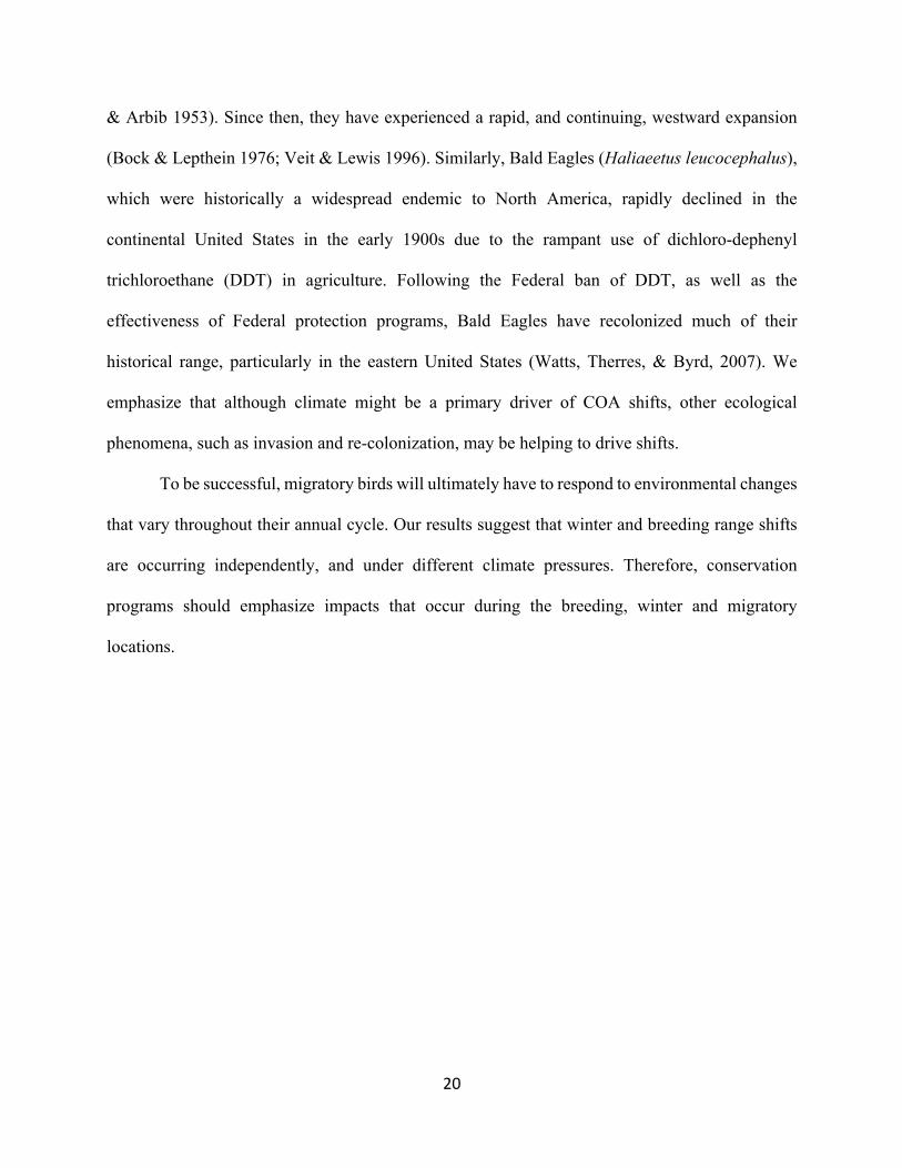
Figure 1.1 - Map of study region in North America with examples of a) unchanged (White-

crowned Sparrow, Zonotrichia leucophrys), b) increased (Savannah Sparrow, Passerculus

sandwichensis) and c) decreased (Brown Thrasher, Toxostoma rufum), migration distances. For

each panel, points in green represent plotted CBC COAs and points in gold are plotted BBS COAs

of each year of the study. Arrows indicate the general direction of the significant shifts that have

resulted in changed migration distance. D1 represents the distance at year 1990 and D2 represents

the distance at year 2015.

22

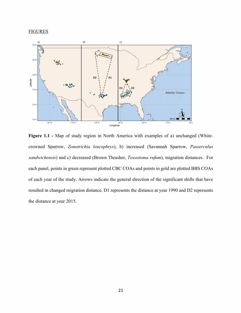
Figure 1.2 - Significant COA shifts (km) in a) wintering range and b) breeding range

from 1990 to 2015. Each arrow represents a single species and the direction and length of the arrow

represents the direction and magnitude of the shift away from its first year COA (0, 0 on the graph).

Arrows above / below the horizontal dashed line indicate northward/ southward movements;

arrows to the right / left of the vertical dashed line represent eastward / westward movements,

respectively.

23

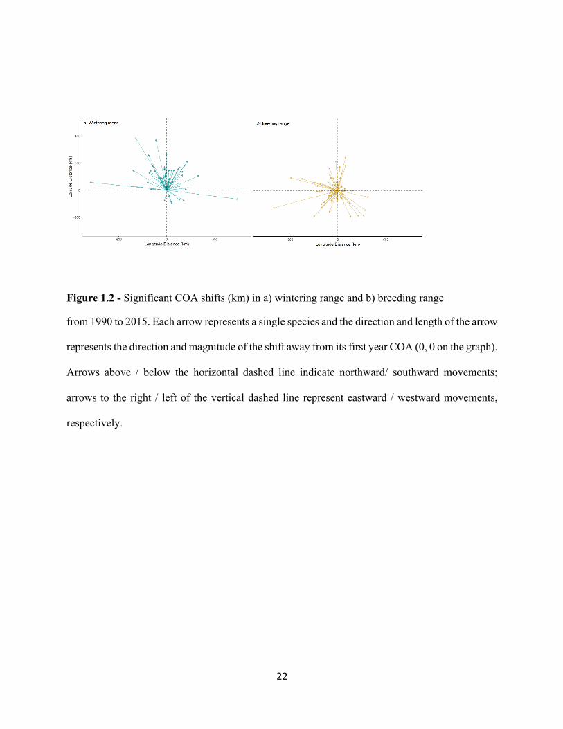
Figure 1.3 – Boxplot of winter and summer latitude shifts (km yr-1) for 77 species of short-distance

migrants. Above the horizontal line indicates northward shifts.

24

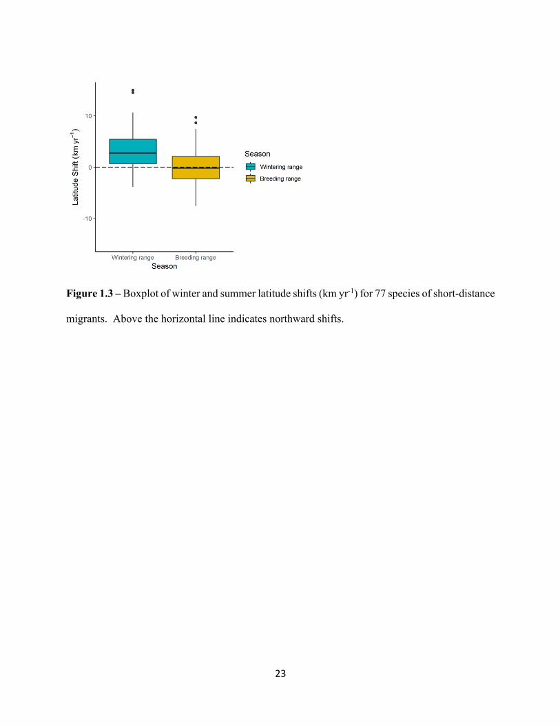
Figure 1.4 - Boxplot of winter and summer longitude shifts (km yr-1) for 77 species of short-

distance migrants. The right of the vertical line indicates eastward shifts.

25

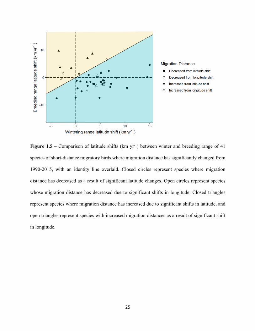
Figure 1.5 – Comparison of latitude shifts (km yr-1) between winter and breeding range of 41

species of short-distance migratory birds where migration distance has significantly changed from

1990-2015, with an identity line overlaid. Closed circles represent species where migration

distance has decreased as a result of significant latitude changes. Open circles represent species

whose migration distance has decreased due to significant shifts in longitude. Closed triangles

represent species where migration distance has increased due to significant shifts in latitude, and

open triangles represent species with increased migration distances as a result of significant shift

in longitude.

26

TABLES

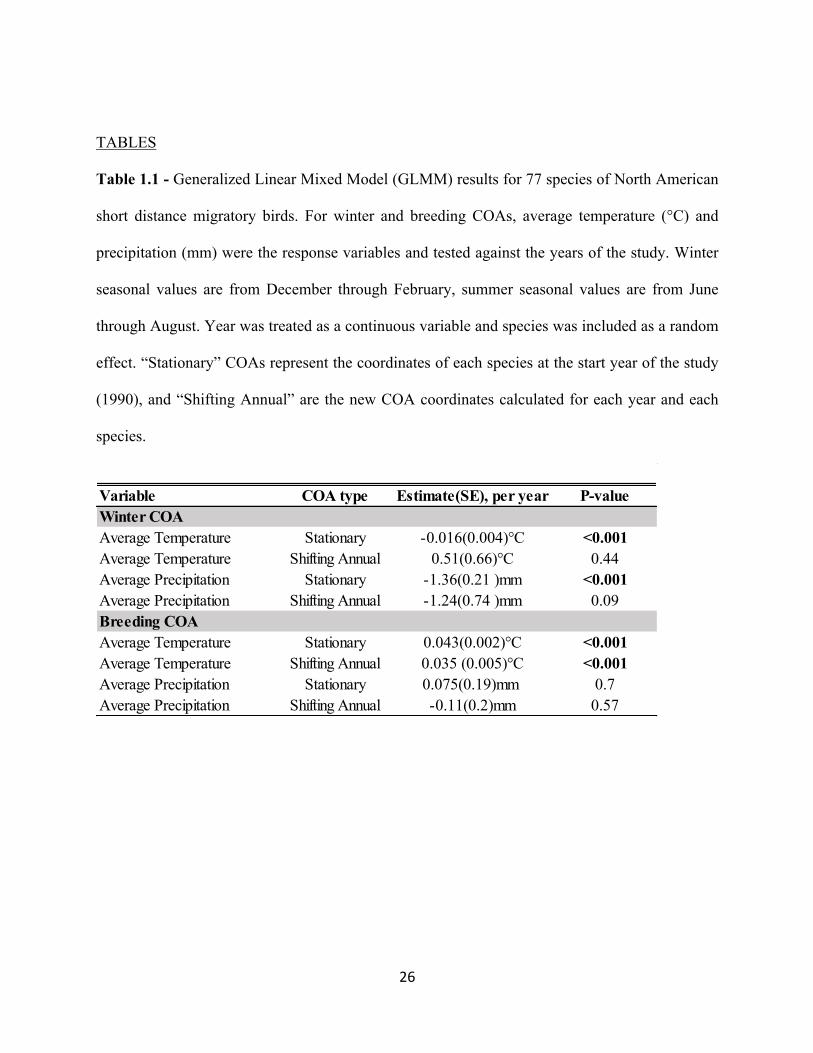
Table 1.1 - Generalized Linear Mixed Model (GLMM) results for 77 species of North American

short distance migratory birds. For winter and breeding COAs, average temperature (°C) and

precipitation (mm) were the response variables and tested against the years of the study. Winter

seasonal values are from December through February, summer seasonal values are from June

through August. Year was treated as a continuous variable and species was included as a random

effect. “Stationary” COAs represent the coordinates of each species at the start year of the study

(1990), and “Shifting Annual” are the new COA coordinates calculated for each year and each

species.

Variable COA type Estimate(SE), per year P-valueWinter COAAverage Temperature Stationary -0.016(0.004)°C <0.001Average Temperature Shifting Annual 0.51(0.66)°C 0.44Average Precipitation Stationary -1.36(0.21 )mm <0.001Average Precipitation Shifting Annual -1.24(0.74 )mm 0.09Breeding COAAverage Temperature Stationary 0.043(0.002)°C <0.001Average Temperature Shifting Annual 0.035 (0.005)°C <0.001Average Precipitation Stationary 0.075(0.19)mm 0.7Average Precipitation Shifting Annual -0.11(0.2)mm 0.57

27

SUPPLEMENTARY TABLES

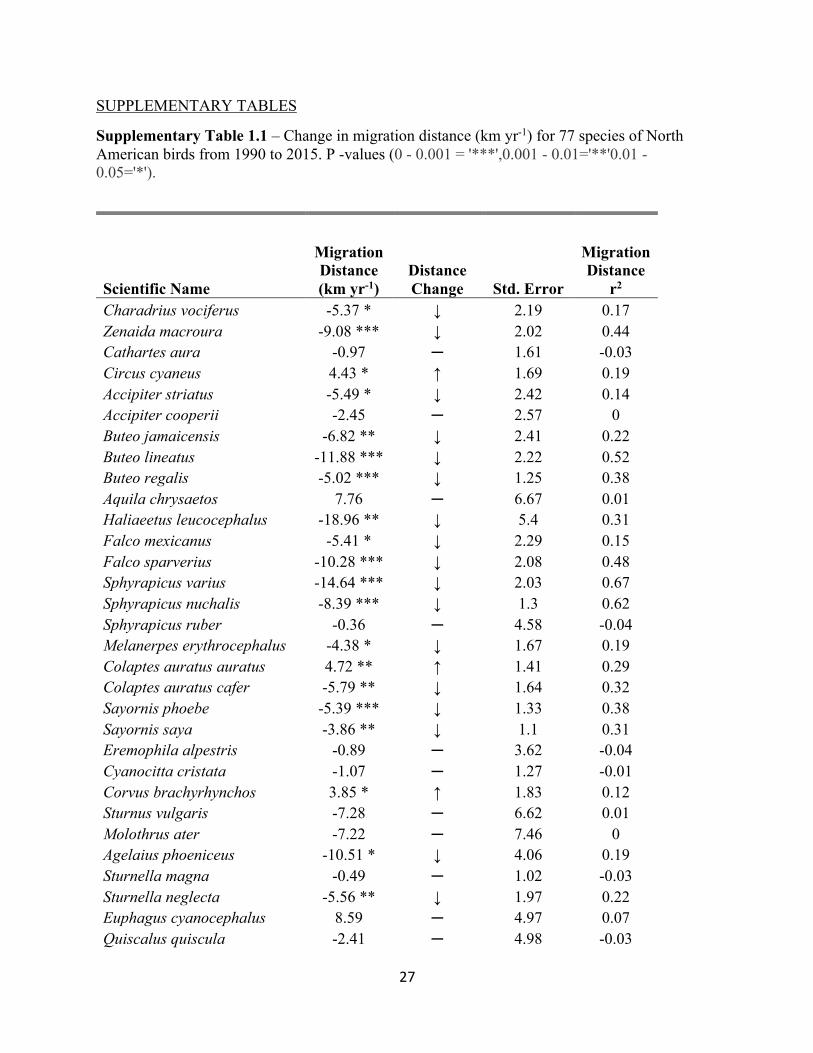
Supplementary Table 1.1 – Change in migration distance (km yr-1) for 77 species of North American birds from 1990 to 2015. P -values (0 - 0.001 = '***',0.001 - 0.01='**'0.01 - 0.05='*').

Scientific Name

Migration Distance (km yr-1)

Distance Change Std. Error

Migration Distance

r2 Charadrius vociferus -5.37 * ↓ 2.19 0.17 Zenaida macroura -9.08 *** ↓ 2.02 0.44 Cathartes aura -0.97 ─ 1.61 -0.03 Circus cyaneus 4.43 * ↑ 1.69 0.19 Accipiter striatus -5.49 * ↓ 2.42 0.14 Accipiter cooperii -2.45 ─ 2.57 0 Buteo jamaicensis -6.82 ** ↓ 2.41 0.22 Buteo lineatus -11.88 *** ↓ 2.22 0.52 Buteo regalis -5.02 *** ↓ 1.25 0.38 Aquila chrysaetos 7.76 ─ 6.67 0.01 Haliaeetus leucocephalus -18.96 ** ↓ 5.4 0.31 Falco mexicanus -5.41 * ↓ 2.29 0.15 Falco sparverius -10.28 *** ↓ 2.08 0.48 Sphyrapicus varius -14.64 *** ↓ 2.03 0.67 Sphyrapicus nuchalis -8.39 *** ↓ 1.3 0.62 Sphyrapicus ruber -0.36 ─ 4.58 -0.04 Melanerpes erythrocephalus -4.38 * ↓ 1.67 0.19 Colaptes auratus auratus 4.72 ** ↑ 1.41 0.29 Colaptes auratus cafer -5.79 ** ↓ 1.64 0.32 Sayornis phoebe -5.39 *** ↓ 1.33 0.38 Sayornis saya -3.86 ** ↓ 1.1 0.31 Eremophila alpestris -0.89 ─ 3.62 -0.04 Cyanocitta cristata -1.07 ─ 1.27 -0.01 Corvus brachyrhynchos 3.85 * ↑ 1.83 0.12 Sturnus vulgaris -7.28 ─ 6.62 0.01 Molothrus ater -7.22 ─ 7.46 0 Agelaius phoeniceus -10.51 * ↓ 4.06 0.19 Sturnella magna -0.49 ─ 1.02 -0.03 Sturnella neglecta -5.56 ** ↓ 1.97 0.22 Euphagus cyanocephalus 8.59 ─ 4.97 0.07 Quiscalus quiscula -2.41 ─ 4.98 -0.03

28

Supplementary Table 1.1 (continued) – Change in migration distance (km yr-1) for 77 species of North American birds from 1990 to 2015. P -values (0 - 0.001 = '***', 0.001 - 0.01='**', 0.01 - 0.05='*'). Haemorhous purpureus -8.47 ─ 4.64 0.09 Haemorhous cassinii -5.68 ─ 6.34 -0.01 Haemorhous mexicanus 5.27 ** ↑ 1.72 0.25 Spinus tristis -9.84 *** ↓ 1.99 0.48 Spinus psaltria -3.54 * ↓ 1.28 0.21 Calcarius ornatus -6.33 ─ 3.44 0.09 Pooecetes gramineus -1.18 ─ 1.35 -0.01 Passerculus sandwichensis 2.16 * ↑ 1.04 0.12 Ammodramus leconteii -10.2 *** ↓ 2.64 0.36 Zonotrichia leucophrys 3.96 ─ 2.26 0.08 Zonotrichia albicollis -3.2 * ↓ 1.17 0.21 Spizella pusilla -2.95 * ↓ 1.33 0.13 Junco hyemalis hyemalis -5.85 ** ↓ 1.96 0.24 Junco hyemalis oreganus -10.18 *** ↓ 1.9 0.53 Junco hyemalis caniceps -4.93 ─ 2.63 0.09 Amphispiza bilineata 0.06 ─ 2.6 -0.04 Peucaea cassinii 0.66 ─ 3.63 -0.04 Melospiza melodia -4.27 *** ↓ 1.12 0.35 Melospiza georgiana -0.9 ─ 1.27 -0.02 Passerella iliaca 12.21 * ↑ 5.62 0.13 Pipilo erythrophthalmus 4.1 ** ↑ 1.1 0.34 Pipilo maculatus -1.68 ─ 1.62 0 Bombycilla cedrorum -3.53 ─ 3.48 0 Lanius ludovicianus 18.06 *** ↑ 3.06 0.57 Setophaga coronata coronata 0.22 ─ 1.49 -0.04 Setophaga coronata auduboni -1.92 ─ 1.34 0.04 Setophaga pinus 12.34 *** ↑ 0.98 0.86 Anthus spragueii 0.52 ─ 4.74 -0.04 Oreoscoptes montanus 3.1 ─ 4.52 -0.02 Toxostoma rufum -8.5 *** ↓ 1.97 0.41 Toxostoma curvirostre -0.3 ─ 1.75 -0.04 Salpinctes obsoletus -5.64 *** ↓ 1.19 0.46 Thryomanes bewickii 10.26 ** ↑ 2.95 0.31 Cistothorus platensis 3.32 ─ 1.61 0.11 Cistothorus palustris 5.98 ─ 3.59 0.07 Certhia americana -9.33 ─ 4.86 0.1 Sitta canadensis -20.14 ** ↓ 5.62 0.32

29

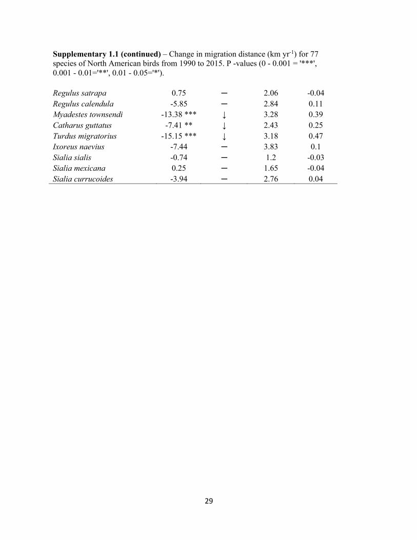
Supplementary 1.1 (continued) – Change in migration distance (km yr-1) for 77 species of North American birds from 1990 to 2015. P -values (0 - 0.001 = '***', 0.001 - 0.01='**', 0.01 - 0.05='*').

Regulus satrapa 0.75 ─ 2.06 -0.04 Regulus calendula -5.85 ─ 2.84 0.11 Myadestes townsendi -13.38 *** ↓ 3.28 0.39 Catharus guttatus -7.41 ** ↓ 2.43 0.25 Turdus migratorius -15.15 *** ↓ 3.18 0.47 Ixoreus naevius -7.44 ─ 3.83 0.1 Sialia sialis -0.74 ─ 1.2 -0.03 Sialia mexicana 0.25 ─ 1.65 -0.04 Sialia currucoides -3.94 ─ 2.76 0.04

30

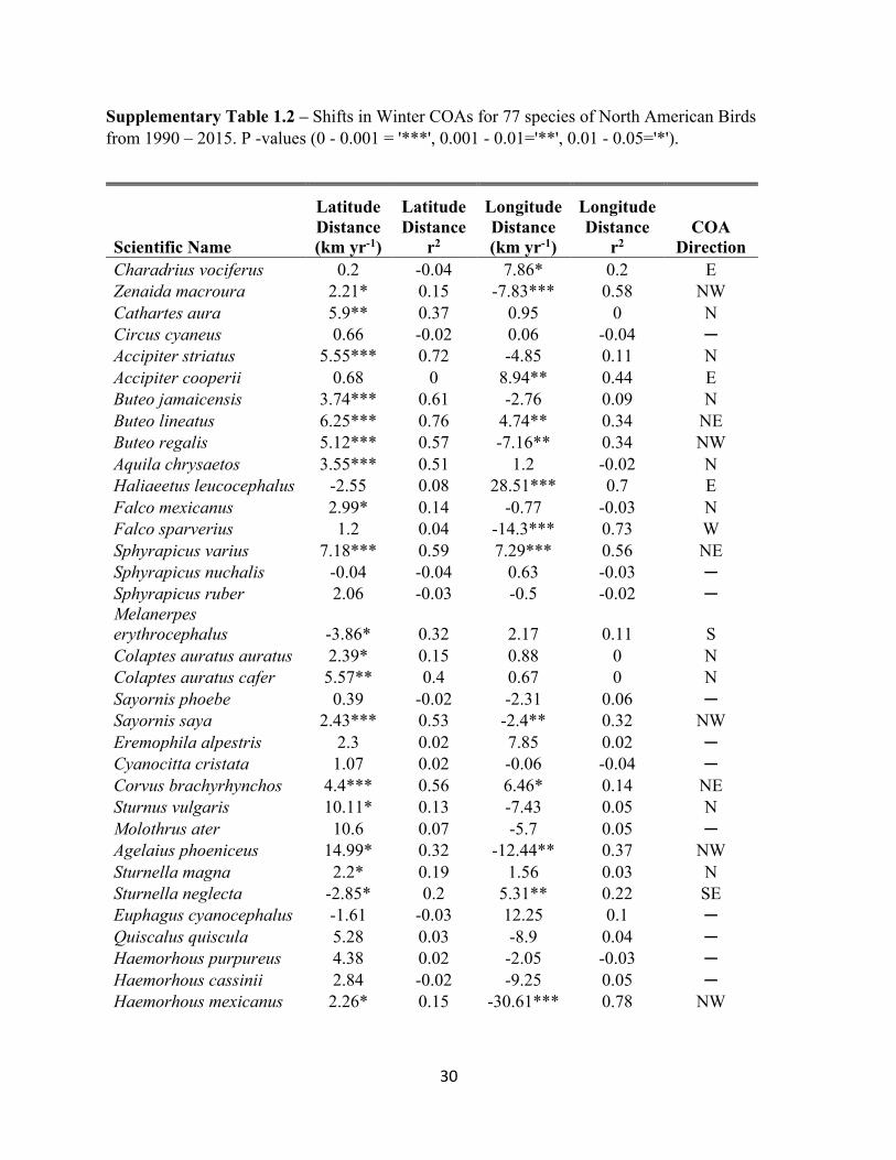
Supplementary Table 1.2 – Shifts in Winter COAs for 77 species of North American Birds from 1990 – 2015. P -values (0 - 0.001 = '***', 0.001 - 0.01='**', 0.01 - 0.05='*').

Scientific Name

Latitude Distance (km yr-1)

Latitude Distance

r2

Longitude Distance (km yr-1)

Longitude Distance

r2 COA

Direction Charadrius vociferus 0.2 -0.04 7.86* 0.2 E Zenaida macroura 2.21* 0.15 -7.83*** 0.58 NW Cathartes aura 5.9** 0.37 0.95 0 N Circus cyaneus 0.66 -0.02 0.06 -0.04 ─ Accipiter striatus 5.55*** 0.72 -4.85 0.11 N Accipiter cooperii 0.68 0 8.94** 0.44 E Buteo jamaicensis 3.74*** 0.61 -2.76 0.09 N Buteo lineatus 6.25*** 0.76 4.74** 0.34 NE Buteo regalis 5.12*** 0.57 -7.16** 0.34 NW Aquila chrysaetos 3.55*** 0.51 1.2 -0.02 N Haliaeetus leucocephalus -2.55 0.08 28.51*** 0.7 E Falco mexicanus 2.99* 0.14 -0.77 -0.03 N Falco sparverius 1.2 0.04 -14.3*** 0.73 W Sphyrapicus varius 7.18*** 0.59 7.29*** 0.56 NE Sphyrapicus nuchalis -0.04 -0.04 0.63 -0.03 ─ Sphyrapicus ruber 2.06 -0.03 -0.5 -0.02 ─ Melanerpes erythrocephalus -3.86* 0.32 2.17 0.11 S Colaptes auratus auratus 2.39* 0.15 0.88 0 N Colaptes auratus cafer 5.57** 0.4 0.67 0 N Sayornis phoebe 0.39 -0.02 -2.31 0.06 ─ Sayornis saya 2.43*** 0.53 -2.4** 0.32 NW Eremophila alpestris 2.3 0.02 7.85 0.02 ─ Cyanocitta cristata 1.07 0.02 -0.06 -0.04 ─ Corvus brachyrhynchos 4.4*** 0.56 6.46* 0.14 NE Sturnus vulgaris 10.11* 0.13 -7.43 0.05 N Molothrus ater 10.6 0.07 -5.7 0.05 ─ Agelaius phoeniceus 14.99* 0.32 -12.44** 0.37 NW Sturnella magna 2.2* 0.19 1.56 0.03 N Sturnella neglecta -2.85* 0.2 5.31** 0.22 SE Euphagus cyanocephalus -1.61 -0.03 12.25 0.1 ─ Quiscalus quiscula 5.28 0.03 -8.9 0.04 ─ Haemorhous purpureus 4.38 0.02 -2.05 -0.03 ─ Haemorhous cassinii 2.84 -0.02 -9.25 0.05 ─ Haemorhous mexicanus 2.26* 0.15 -30.61*** 0.78 NW

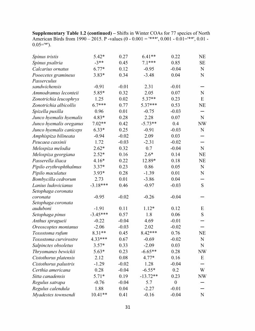
31

Supplementary Table 1.2 (continued) – Shifts in Winter COAs for 77 species of North American Birds from 1990 – 2015. P -values (0 - 0.001 = '***', 0.001 - 0.01='**', 0.01 - 0.05='*'). Spinus tristis 5.42* 0.27 6.41** 0.22 NE Spinus psaltria -3** 0.45 7.1*** 0.85 SE Calcarius ornatus 6.77* 0.12 -0.95 -0.04 N Pooecetes gramineus 3.83* 0.34 -3.48 0.04 N Passerculus sandwichensis -0.91 -0.01 2.31 -0.01 ─ Ammodramus leconteii 5.85* 0.32 2.05 0.07 N Zonotrichia leucophrys 1.25 0.02 5.37** 0.23 E Zonotrichia albicollis 6.7*** 0.77 5.37*** 0.53 NE Spizella pusilla 0.96 0.01 -0.75 -0.03 ─ Junco hyemalis hyemalis 4.83* 0.28 2.28 0.07 N Junco hyemalis oreganus 7.02** 0.42 -5.73** 0.4 NW Junco hyemalis caniceps 6.33* 0.25 -0.91 -0.03 N Amphispiza bilineata -0.94 -0.02 2.09 0.03 ─ Peucaea cassinii 1.72 -0.03 -2.31 -0.02 ─ Melospiza melodia 2.62* 0.32 0.7 -0.04 N Melospiza georgiana 2.52* 0.16 2.6* 0.14 NE Passerella iliaca 4.16* 0.22 12.89* 0.18 NE Pipilo erythrophthalmus 3.37* 0.23 0.86 0.05 N Pipilo maculatus 3.93* 0.28 -1.39 0.01 N Bombycilla cedrorum 2.73 0.01 -3.86 0.04 ─ Lanius ludovicianus -3.18*** 0.46 -0.97 -0.03 S Setophaga coronata coronata -0.95 -0.02 -0.26 -0.04 ─ Setophaga coronata auduboni -1.91 0.11 1.12* 0.12 E Setophaga pinus -3.45*** 0.57 1.8 0.06 S Anthus spragueii -0.22 -0.04 4.69 -0.01 ─ Oreoscoptes montanus -2.06 -0.03 2.02 -0.02 ─ Toxostoma rufum 8.31** 0.45 8.42*** 0.76 NE Toxostoma curvirostre 4.33*** 0.67 -0.69 -0.02 N Salpinctes obsoletus 3.57* 0.33 -2.09 0.03 N Thryomanes bewickii 5.63* 0.23 -6.65** 0.28 NW Cistothorus platensis 2.12 0.08 4.77* 0.16 E Cistothorus palustris -1.29 -0.02 1.28 -0.04 ─ Certhia americana 0.28 -0.04 -6.55* 0.2 W Sitta canadensis 5.71* 0.19 -13.72** 0.23 NW Regulus satrapa -0.76 -0.04 5.7 0 ─ Regulus calendula 1.88 0.04 -2.27 -0.01 ─ Myadestes townsendi 10.41** 0.41 -0.16 -0.04 N

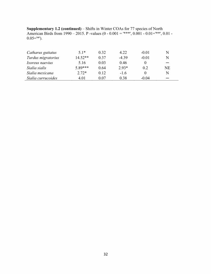
32

Supplementary 1.2 (continued) – Shifts in Winter COAs for 77 species of North American Birds from 1990 – 2015. P -values (0 - 0.001 = '***', 0.001 - 0.01='**', 0.01 - 0.05='*'). Catharus guttatus 5.1* 0.32 4.22 -0.01 N Turdus migratorius 14.52** 0.37 -4.39 -0.01 N Ixoreus naevius 5.16 0.03 0.46 0 ─ Sialia sialis 5.89*** 0.64 2.93* 0.2 NE Sialia mexicana 2.72* 0.12 -1.6 0 N Sialia currucoides 4.01 0.07 0.38 -0.04 ─

33

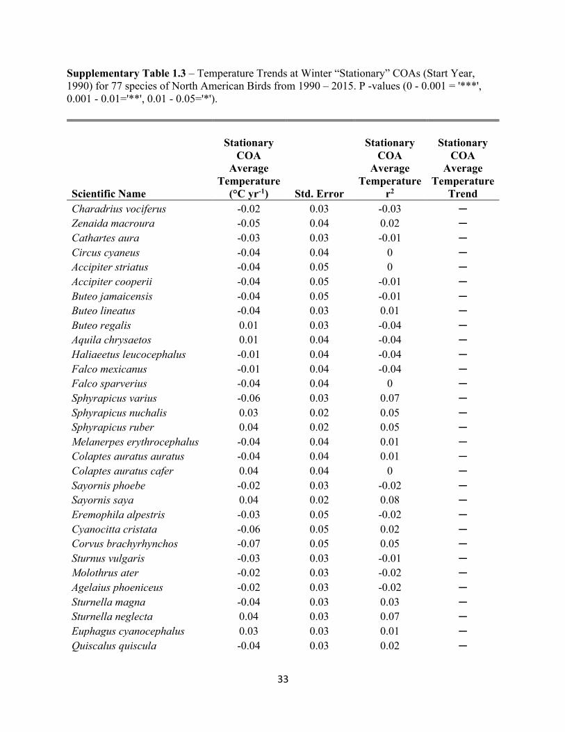
Supplementary Table 1.3 – Temperature Trends at Winter “Stationary” COAs (Start Year, 1990) for 77 species of North American Birds from 1990 – 2015. P -values (0 - 0.001 = '***', 0.001 - 0.01='**', 0.01 - 0.05='*').

Scientific Name

Stationary COA

Average Temperature

(°C yr-1) Std. Error

Stationary COA

Average Temperature

r2

Stationary COA

Average Temperature

Trend Charadrius vociferus -0.02 0.03 -0.03 ─ Zenaida macroura -0.05 0.04 0.02 ─ Cathartes aura -0.03 0.03 -0.01 ─ Circus cyaneus -0.04 0.04 0 ─ Accipiter striatus -0.04 0.05 0 ─ Accipiter cooperii -0.04 0.05 -0.01 ─ Buteo jamaicensis -0.04 0.05 -0.01 ─ Buteo lineatus -0.04 0.03 0.01 ─ Buteo regalis 0.01 0.03 -0.04 ─ Aquila chrysaetos 0.01 0.04 -0.04 ─ Haliaeetus leucocephalus -0.01 0.04 -0.04 ─ Falco mexicanus -0.01 0.04 -0.04 ─ Falco sparverius -0.04 0.04 0 ─ Sphyrapicus varius -0.06 0.03 0.07 ─ Sphyrapicus nuchalis 0.03 0.02 0.05 ─ Sphyrapicus ruber 0.04 0.02 0.05 ─ Melanerpes erythrocephalus -0.04 0.04 0.01 ─ Colaptes auratus auratus -0.04 0.04 0.01 ─ Colaptes auratus cafer 0.04 0.04 0 ─ Sayornis phoebe -0.02 0.03 -0.02 ─ Sayornis saya 0.04 0.02 0.08 ─ Eremophila alpestris -0.03 0.05 -0.02 ─ Cyanocitta cristata -0.06 0.05 0.02 ─ Corvus brachyrhynchos -0.07 0.05 0.05 ─ Sturnus vulgaris -0.03 0.03 -0.01 ─ Molothrus ater -0.02 0.03 -0.02 ─ Agelaius phoeniceus -0.02 0.03 -0.02 ─ Sturnella magna -0.04 0.03 0.03 ─ Sturnella neglecta 0.04 0.03 0.07 ─ Euphagus cyanocephalus 0.03 0.03 0.01 ─ Quiscalus quiscula -0.04 0.03 0.02 ─

34

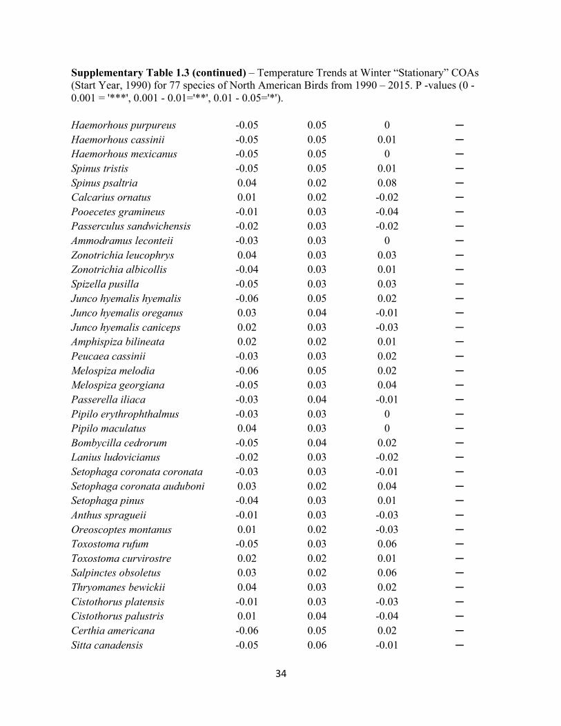
Supplementary Table 1.3 (continued) – Temperature Trends at Winter “Stationary” COAs (Start Year, 1990) for 77 species of North American Birds from 1990 – 2015. P -values (0 - 0.001 = '***', 0.001 - 0.01='**', 0.01 - 0.05='*'). Haemorhous purpureus -0.05 0.05 0 ─ Haemorhous cassinii -0.05 0.05 0.01 ─ Haemorhous mexicanus -0.05 0.05 0 ─ Spinus tristis -0.05 0.05 0.01 ─ Spinus psaltria 0.04 0.02 0.08 ─ Calcarius ornatus 0.01 0.02 -0.02 ─ Pooecetes gramineus -0.01 0.03 -0.04 ─ Passerculus sandwichensis -0.02 0.03 -0.02 ─ Ammodramus leconteii -0.03 0.03 0 ─ Zonotrichia leucophrys 0.04 0.03 0.03 ─ Zonotrichia albicollis -0.04 0.03 0.01 ─ Spizella pusilla -0.05 0.03 0.03 ─ Junco hyemalis hyemalis -0.06 0.05 0.02 ─ Junco hyemalis oreganus 0.03 0.04 -0.01 ─ Junco hyemalis caniceps 0.02 0.03 -0.03 ─ Amphispiza bilineata 0.02 0.02 0.01 ─ Peucaea cassinii -0.03 0.03 0.02 ─ Melospiza melodia -0.06 0.05 0.02 ─ Melospiza georgiana -0.05 0.03 0.04 ─ Passerella iliaca -0.03 0.04 -0.01 ─ Pipilo erythrophthalmus -0.03 0.03 0 ─ Pipilo maculatus 0.04 0.03 0 ─ Bombycilla cedrorum -0.05 0.04 0.02 ─ Lanius ludovicianus -0.02 0.03 -0.02 ─ Setophaga coronata coronata -0.03 0.03 -0.01 ─ Setophaga coronata auduboni 0.03 0.02 0.04 ─ Setophaga pinus -0.04 0.03 0.01 ─ Anthus spragueii -0.01 0.03 -0.03 ─ Oreoscoptes montanus 0.01 0.02 -0.03 ─ Toxostoma rufum -0.05 0.03 0.06 ─ Toxostoma curvirostre 0.02 0.02 0.01 ─ Salpinctes obsoletus 0.03 0.02 0.06 ─ Thryomanes bewickii 0.04 0.03 0.02 ─ Cistothorus platensis -0.01 0.03 -0.03 ─ Cistothorus palustris 0.01 0.04 -0.04 ─ Certhia americana -0.06 0.05 0.02 ─ Sitta canadensis -0.05 0.06 -0.01 ─

35

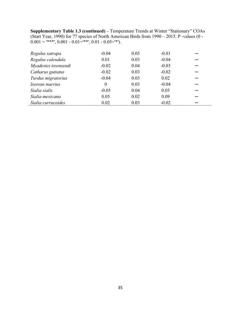
Supplementary Table 1.3 (continued) – Temperature Trends at Winter “Stationary” COAs (Start Year, 1990) for 77 species of North American Birds from 1990 – 2015. P -values (0 - 0.001 = '***', 0.001 - 0.01='**', 0.01 - 0.05='*'). Regulus satrapa -0.04 0.05 -0.01 ─ Regulus calendula 0.01 0.03 -0.04 ─ Myadestes townsendi -0.02 0.04 -0.03 ─ Catharus guttatus -0.02 0.03 -0.02 ─ Turdus migratorius -0.04 0.03 0.02 ─ Ixoreus naevius 0 0.03 -0.04 ─ Sialia sialis -0.05 0.04 0.03 ─ Sialia mexicana 0.05 0.02 0.09 ─ Sialia currucoides 0.02 0.03 -0.02 ─

36

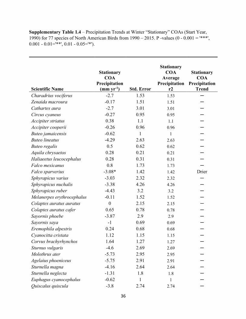
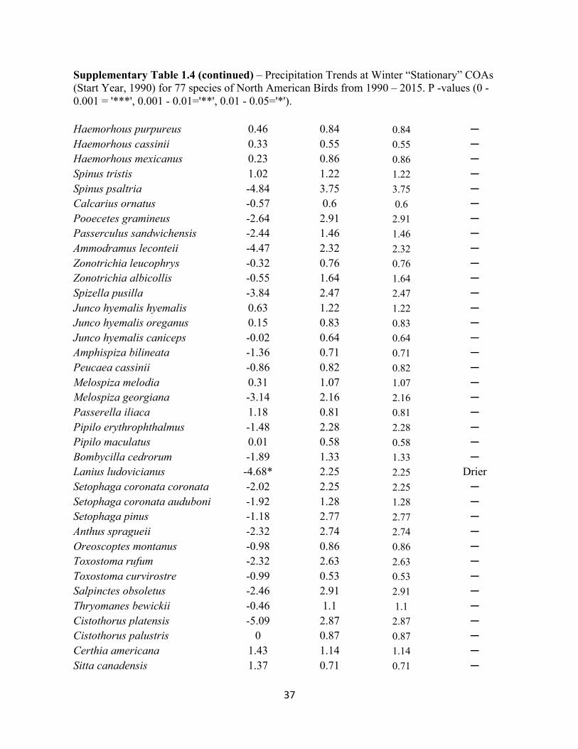
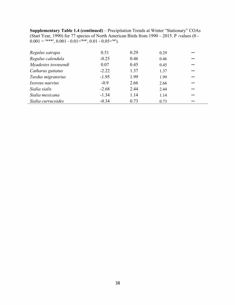
Supplementary Table 1.4 – Precipitation Trends at Winter “Stationary” COAs (Start Year, 1990) for 77 species of North American Birds from 1990 – 2015. P -values (0 - 0.001 = '***', 0.001 - 0.01='**', 0.01 - 0.05='*').

Scientific Name

Stationary COA

Precipitation (mm yr-1) Std. Error

Stationary COA

Average Precipitation

r2

Stationary COA

Precipitation Trend

Charadrius vociferus -2.7 1.53 1.53 ─ Zenaida macroura -0.17 1.51 1.51 ─ Cathartes aura -2.7 3.01 3.01 ─ Circus cyaneus -0.27 0.95 0.95 ─ Accipiter striatus 0.38 1.1 1.1 ─ Accipiter cooperii -0.26 0.96 0.96 ─ Buteo jamaicensis -0.62 1 1 ─ Buteo lineatus -4.29 2.63 2.63 ─ Buteo regalis 0.5 0.62 0.62 ─ Aquila chrysaetos 0.28 0.21 0.21 ─ Haliaeetus leucocephalus 0.28 0.31 0.31 ─ Falco mexicanus 0.8 1.73 1.73 ─ Falco sparverius -3.08* 1.42 1.42 Drier Sphyrapicus varius -3.03 2.32 2.32 ─ Sphyrapicus nuchalis -3.38 4.26 4.26 ─ Sphyrapicus ruber -4.43 3.2 3.2 ─ Melanerpes erythrocephalus -0.11 1.52 1.52 ─ Colaptes auratus auratus 0 2.15 2.15 ─ Colaptes auratus cafer 0.65 0.78 0.78 ─ Sayornis phoebe -3.87 2.9 2.9 ─ Sayornis saya -1 0.69 0.69 ─ Eremophila alpestris 0.24 0.68 0.68 ─ Cyanocitta cristata 1.12 1.15 1.15 ─ Corvus brachyrhynchos 1.64 1.27 1.27 ─ Sturnus vulgaris -4.6 2.69 2.69 ─ Molothrus ater -5.73 2.95 2.95 ─ Agelaius phoeniceus -5.75 2.91 2.91 ─ Sturnella magna -4.16 2.64 2.64 ─ Sturnella neglecta -1.31 1.8 1.8 ─ Euphagus cyanocephalus -0.62 1 1 ─ Quiscalus quiscula -3.8 2.74 2.74 ─

37

Supplementary Table 1.4 (continued) – Precipitation Trends at Winter “Stationary” COAs (Start Year, 1990) for 77 species of North American Birds from 1990 – 2015. P -values (0 - 0.001 = '***', 0.001 - 0.01='**', 0.01 - 0.05='*'). Haemorhous purpureus 0.46 0.84 0.84 ─ Haemorhous cassinii 0.33 0.55 0.55 ─ Haemorhous mexicanus 0.23 0.86 0.86 ─ Spinus tristis 1.02 1.22 1.22 ─ Spinus psaltria -4.84 3.75 3.75 ─ Calcarius ornatus -0.57 0.6 0.6 ─ Pooecetes gramineus -2.64 2.91 2.91 ─ Passerculus sandwichensis -2.44 1.46 1.46 ─ Ammodramus leconteii -4.47 2.32 2.32 ─ Zonotrichia leucophrys -0.32 0.76 0.76 ─ Zonotrichia albicollis -0.55 1.64 1.64 ─ Spizella pusilla -3.84 2.47 2.47 ─ Junco hyemalis hyemalis 0.63 1.22 1.22 ─ Junco hyemalis oreganus 0.15 0.83 0.83 ─ Junco hyemalis caniceps -0.02 0.64 0.64 ─ Amphispiza bilineata -1.36 0.71 0.71 ─ Peucaea cassinii -0.86 0.82 0.82 ─ Melospiza melodia 0.31 1.07 1.07 ─ Melospiza georgiana -3.14 2.16 2.16 ─ Passerella iliaca 1.18 0.81 0.81 ─ Pipilo erythrophthalmus -1.48 2.28 2.28 ─ Pipilo maculatus 0.01 0.58 0.58 ─ Bombycilla cedrorum -1.89 1.33 1.33 ─ Lanius ludovicianus -4.68* 2.25 2.25 Drier Setophaga coronata coronata -2.02 2.25 2.25 ─ Setophaga coronata auduboni -1.92 1.28 1.28 ─ Setophaga pinus -1.18 2.77 2.77 ─ Anthus spragueii -2.32 2.74 2.74 ─ Oreoscoptes montanus -0.98 0.86 0.86 ─ Toxostoma rufum -2.32 2.63 2.63 ─ Toxostoma curvirostre -0.99 0.53 0.53 ─ Salpinctes obsoletus -2.46 2.91 2.91 ─ Thryomanes bewickii -0.46 1.1 1.1 ─ Cistothorus platensis -5.09 2.87 2.87 ─ Cistothorus palustris 0 0.87 0.87 ─ Certhia americana 1.43 1.14 1.14 ─ Sitta canadensis 1.37 0.71 0.71 ─

38

Supplementary Table 1.4 (continued) – Precipitation Trends at Winter “Stationary” COAs (Start Year, 1990) for 77 species of North American Birds from 1990 – 2015. P -values (0 - 0.001 = '***', 0.001 - 0.01='**', 0.01 - 0.05='*'). Regulus satrapa 0.51 0.29 0.29 ─ Regulus calendula -0.25 0.46 0.46 ─ Myadestes townsendi 0.07 0.45 0.45 ─ Catharus guttatus -2.22 1.37 1.37 ─ Turdus migratorius -1.95 1.99 1.99 ─ Ixoreus naevius -0.9 2.66 2.66 ─ Sialia sialis -2.68 2.44 2.44 ─ Sialia mexicana -1.34 1.14 1.14 ─ Sialia currucoides -0.34 0.73 0.73 ─

39

Supplementary Table 1.5 – Temperature Trends at Winter “Shifting Annual” COAs (Start Year, 1990) for 77 species of North American Birds from 1990 – 2015. P -values (0 - 0.001 = '***', 0.001 - 0.01='**', 0.01 - 0.05='*').

Scientific Name

Shifting Annual COA

Average Temperature

(°C yr-1) Std. Error

Shifting Annual COA

Average Temperature

r2

Shifting Annual COA

Average Temperature

Trend Charadrius vociferus 0.01 0.04 -0.04 ─ Zenaida macroura -0.1* 0.04 0.14 Cooler Cathartes aura -0.13*** 0.03 0.39 Cooler Circus cyaneus -0.04 0.04 0.01 ─ Accipiter striatus -0.13* 0.05 0.19 Cooler Accipiter cooperii -0.04 0.05 -0.02 ─ Buteo jamaicensis -0.1* 0.05 0.12 Cooler Buteo lineatus -0.11** 0.04 0.23 Cooler Buteo regalis -0.11 0.07 0.05 ─ Aquila chrysaetos -0.09 0.05 0.06 ─ Haliaeetus leucocephalus -0.1 0.06 0.08 ─ Falco mexicanus 0.02 0.06 -0.04 ─ Falco sparverius -0.04 0.04 0.01 ─ Sphyrapicus varius -0.14** 0.04 0.27 Cooler Sphyrapicus nuchalis 0.04 0.07 -0.03 ─ Sphyrapicus ruber -0.07 0.07 0 ─ Melanerpes erythrocephalus 0 0.04 -0.04 ─ Colaptes auratus auratus -0.06 0.04 0.05 ─ Colaptes auratus cafer -0.04 0.05 -0.02 ─ Sayornis phoebe -0.03 0.03 -0.02 ─ Sayornis saya -0.04 0.03 0.03 ─ Eremophila alpestris -0.06 0.06 0 ─ Cyanocitta cristata -0.07 0.05 0.03 ─ Corvus brachyrhynchos -0.09 0.05 0.11 ─ Sturnus vulgaris -0.17* 0.07 0.18 Cooler Molothrus ater -0.15* 0.07 0.13 Cooler Agelaius phoeniceus -0.19** 0.05 0.34 Cooler Sturnella magna -0.08* 0.04 0.13 Cooler Sturnella neglecta 0.14 0.08 0.09 ─ Euphagus cyanocephalus -0.17* 0.07 0.17 Cooler Quiscalus quiscula -0.07 0.06 0.01 ─

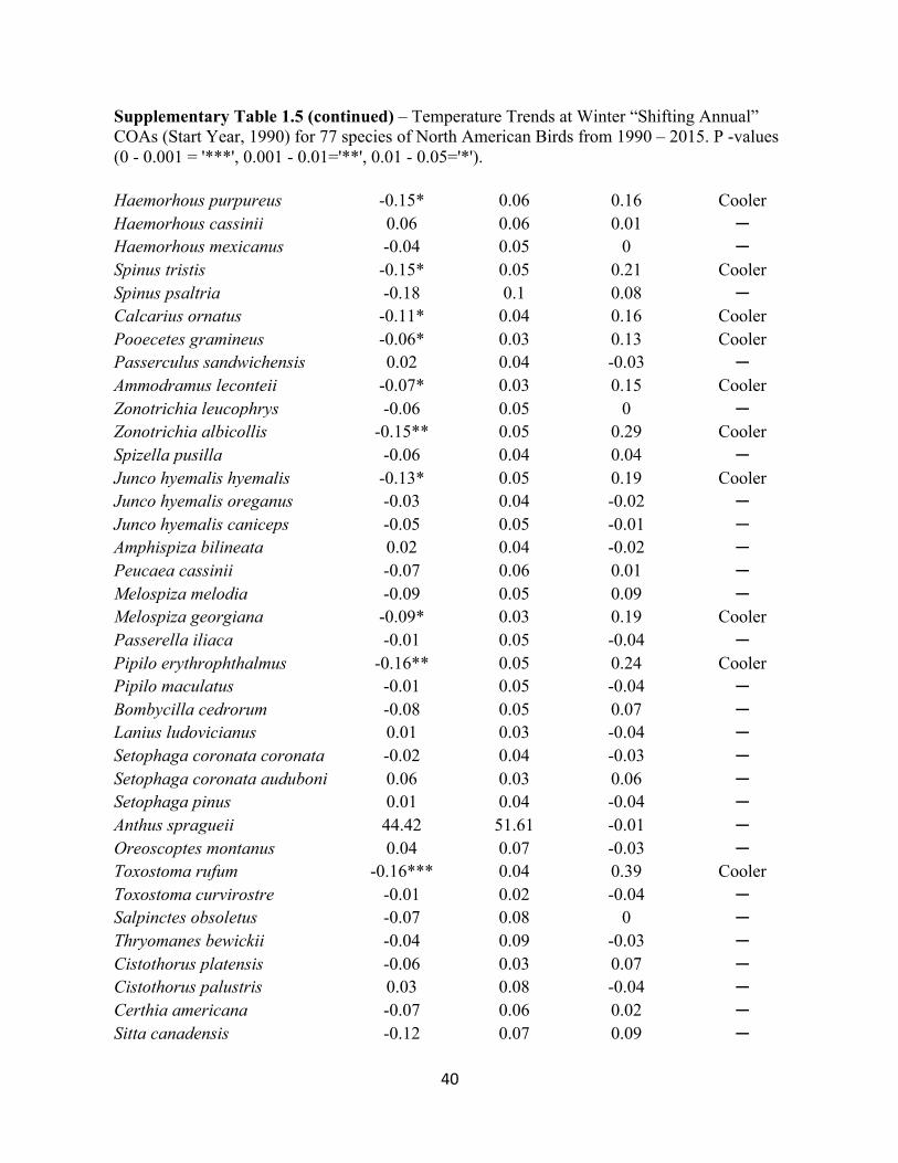
40

Supplementary Table 1.5 (continued) – Temperature Trends at Winter “Shifting Annual” COAs (Start Year, 1990) for 77 species of North American Birds from 1990 – 2015. P -values (0 - 0.001 = '***', 0.001 - 0.01='**', 0.01 - 0.05='*'). Haemorhous purpureus -0.15* 0.06 0.16 Cooler Haemorhous cassinii 0.06 0.06 0.01 ─ Haemorhous mexicanus -0.04 0.05 0 ─ Spinus tristis -0.15* 0.05 0.21 Cooler Spinus psaltria -0.18 0.1 0.08 ─ Calcarius ornatus -0.11* 0.04 0.16 Cooler Pooecetes gramineus -0.06* 0.03 0.13 Cooler Passerculus sandwichensis 0.02 0.04 -0.03 ─ Ammodramus leconteii -0.07* 0.03 0.15 Cooler Zonotrichia leucophrys -0.06 0.05 0 ─ Zonotrichia albicollis -0.15** 0.05 0.29 Cooler Spizella pusilla -0.06 0.04 0.04 ─ Junco hyemalis hyemalis -0.13* 0.05 0.19 Cooler Junco hyemalis oreganus -0.03 0.04 -0.02 ─ Junco hyemalis caniceps -0.05 0.05 -0.01 ─ Amphispiza bilineata 0.02 0.04 -0.02 ─ Peucaea cassinii -0.07 0.06 0.01 ─ Melospiza melodia -0.09 0.05 0.09 ─ Melospiza georgiana -0.09* 0.03 0.19 Cooler Passerella iliaca -0.01 0.05 -0.04 ─ Pipilo erythrophthalmus -0.16** 0.05 0.24 Cooler Pipilo maculatus -0.01 0.05 -0.04 ─ Bombycilla cedrorum -0.08 0.05 0.07 ─ Lanius ludovicianus 0.01 0.03 -0.04 ─ Setophaga coronata coronata -0.02 0.04 -0.03 ─ Setophaga coronata auduboni 0.06 0.03 0.06 ─ Setophaga pinus 0.01 0.04 -0.04 ─ Anthus spragueii 44.42 51.61 -0.01 ─ Oreoscoptes montanus 0.04 0.07 -0.03 ─ Toxostoma rufum -0.16*** 0.04 0.39 Cooler Toxostoma curvirostre -0.01 0.02 -0.04 ─ Salpinctes obsoletus -0.07 0.08 0 ─ Thryomanes bewickii -0.04 0.09 -0.03 ─ Cistothorus platensis -0.06 0.03 0.07 ─ Cistothorus palustris 0.03 0.08 -0.04 ─ Certhia americana -0.07 0.06 0.02 ─ Sitta canadensis -0.12 0.07 0.09 ─

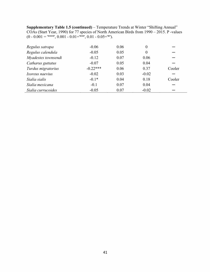
41

Supplementary Table 1.5 (continued) – Temperature Trends at Winter “Shifting Annual” COAs (Start Year, 1990) for 77 species of North American Birds from 1990 – 2015. P -values (0 - 0.001 = '***', 0.001 - 0.01='**', 0.01 - 0.05='*'). Regulus satrapa -0.06 0.06 0 ─ Regulus calendula -0.05 0.05 0 ─ Myadestes townsendi -0.12 0.07 0.06 ─ Catharus guttatus -0.07 0.05 0.04 ─ Turdus migratorius -0.22*** 0.06 0.37 Cooler Ixoreus naevius -0.02 0.03 -0.02 ─ Sialia sialis -0.1* 0.04 0.18 Cooler Sialia mexicana -0.1 0.07 0.04 ─ Sialia currucoides -0.05 0.07 -0.02 ─

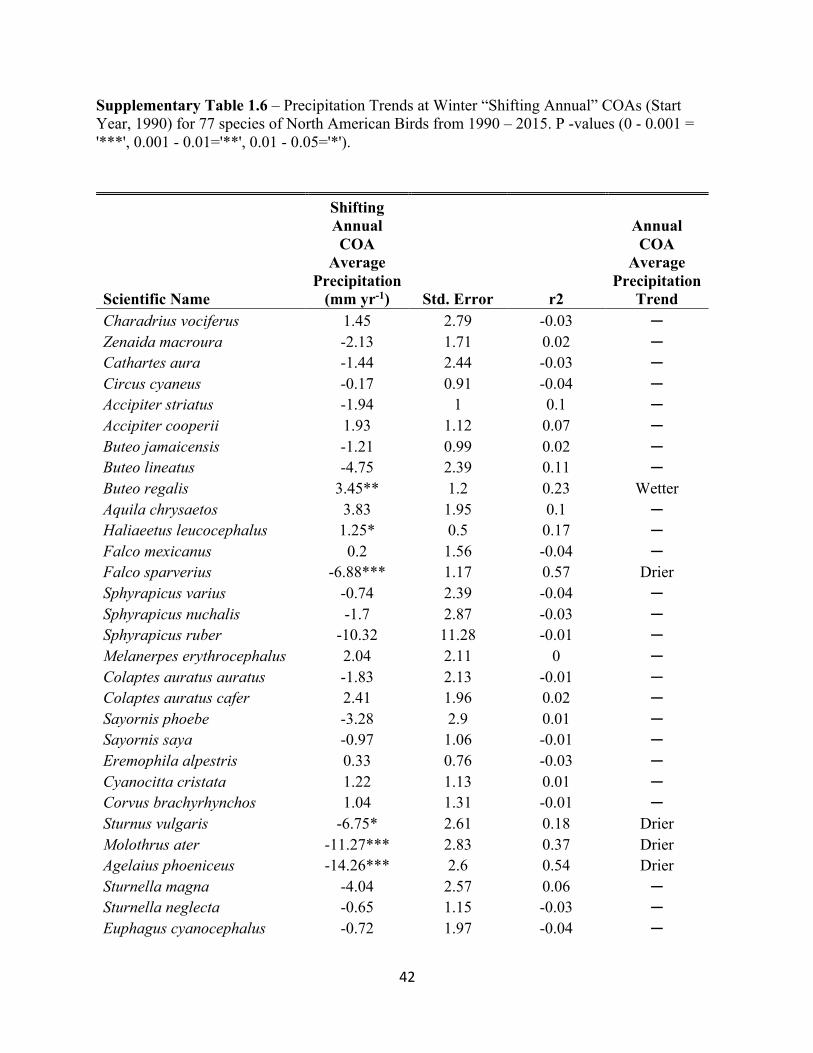
42

Supplementary Table 1.6 – Precipitation Trends at Winter “Shifting Annual” COAs (Start Year, 1990) for 77 species of North American Birds from 1990 – 2015. P -values (0 - 0.001 = '***', 0.001 - 0.01='**', 0.01 - 0.05='*').

Scientific Name

Shifting Annual COA

Average Precipitation

(mm yr-1) Std. Error r2

Annual COA

Average Precipitation

Trend Charadrius vociferus 1.45 2.79 -0.03 ─ Zenaida macroura -2.13 1.71 0.02 ─ Cathartes aura -1.44 2.44 -0.03 ─ Circus cyaneus -0.17 0.91 -0.04 ─ Accipiter striatus -1.94 1 0.1 ─ Accipiter cooperii 1.93 1.12 0.07 ─ Buteo jamaicensis -1.21 0.99 0.02 ─ Buteo lineatus -4.75 2.39 0.11 ─ Buteo regalis 3.45** 1.2 0.23 Wetter Aquila chrysaetos 3.83 1.95 0.1 ─ Haliaeetus leucocephalus 1.25* 0.5 0.17 ─ Falco mexicanus 0.2 1.56 -0.04 ─ Falco sparverius -6.88*** 1.17 0.57 Drier Sphyrapicus varius -0.74 2.39 -0.04 ─ Sphyrapicus nuchalis -1.7 2.87 -0.03 ─ Sphyrapicus ruber -10.32 11.28 -0.01 ─ Melanerpes erythrocephalus 2.04 2.11 0 ─ Colaptes auratus auratus -1.83 2.13 -0.01 ─ Colaptes auratus cafer 2.41 1.96 0.02 ─ Sayornis phoebe -3.28 2.9 0.01 ─ Sayornis saya -0.97 1.06 -0.01 ─ Eremophila alpestris 0.33 0.76 -0.03 ─ Cyanocitta cristata 1.22 1.13 0.01 ─ Corvus brachyrhynchos 1.04 1.31 -0.01 ─ Sturnus vulgaris -6.75* 2.61 0.18 Drier Molothrus ater -11.27*** 2.83 0.37 Drier Agelaius phoeniceus -14.26*** 2.6 0.54 Drier Sturnella magna -4.04 2.57 0.06 ─ Sturnella neglecta -0.65 1.15 -0.03 ─ Euphagus cyanocephalus -0.72 1.97 -0.04 ─

43

Supplementary Table 1.6 (continued) – Precipitation Trends at Winter “Shifting Annual” COAs (Start Year, 1990) for 77 species of North American Birds from 1990 – 2015. P -values (0 - 0.001 = '***', 0.001 - 0.01='**', 0.01 - 0.05='*').

Quiscalus quiscula -6.4* 3.09 0.12 Drier Haemorhous purpureus 0.12 1.11 -0.04 ─ Haemorhous cassinii 1.52 1.01 0.05 ─ Haemorhous mexicanus -2.92*** 0.68 0.41 Drier Spinus tristis 1.19 1.25 0 ─ Spinus psaltria -20.73* 7.82 0.19 Drier Calcarius ornatus -0.18 0.78 -0.04 ─ Pooecetes gramineus -4.09 2.66 0.05 ─ Passerculus sandwichensis -2.31 2.33 0 ─ Ammodramus leconteii -5.45* 2.57 0.12 Drier Zonotrichia leucophrys -1.16 1.39 -0.01 ─ Zonotrichia albicollis -2.67 2.07 0.03 ─ Spizella pusilla -3.44 2.65 0.03 ─ Junco hyemalis hyemalis -0.05 1.27 -0.04 ─ Junco hyemalis oreganus -1.14 1.22 -0.01 ─ Junco hyemalis caniceps -1.58 1.51 0 ─ Amphispiza bilineata -2.24* 0.92 0.17 Drier Peucaea cassinii -0.57 1.06 -0.03 ─ Melospiza melodia -0.66 0.98 -0.02 ─ Melospiza georgiana 0.47 2.56 -0.04 ─ Passerella iliaca -3.7* 1.76 0.12 Drier Pipilo erythrophthalmus 1.54 3.02 -0.03 ─ Pipilo maculatus 0.43 1.23 -0.04 ─ Bombycilla cedrorum -3.45* 1.31 0.19 Drier Lanius ludovicianus -4.44 2.68 0.07 ─ Setophaga coronata coronata -1.01 2.04 -0.03 ─ Setophaga coronata auduboni -2.85 1.49 0.1 ─ Setophaga pinus -1.38 2.58 -0.03 ─ Anthus spragueii 43.92 52.69 -0.01 ─ Oreoscoptes montanus -0.21 0.96 -0.04 ─ Toxostoma rufum -2.48 2.41 0 ─ Toxostoma curvirostre -0.95 0.6 0.06 ─ Salpinctes obsoletus -1.07 2.59 -0.03 ─ Thryomanes bewickii -3.23 1.7 0.09 ─ Cistothorus platensis -3.09 3.19 0 ─ Cistothorus palustris 2.28 2.19 0 ─ Certhia americana -0.42 0.98 -0.03 ─

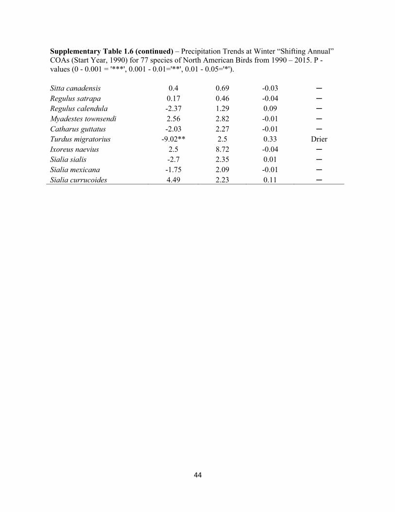
44

Supplementary Table 1.6 (continued) – Precipitation Trends at Winter “Shifting Annual” COAs (Start Year, 1990) for 77 species of North American Birds from 1990 – 2015. P -values (0 - 0.001 = '***', 0.001 - 0.01='**', 0.01 - 0.05='*'). Sitta canadensis 0.4 0.69 -0.03 ─ Regulus satrapa 0.17 0.46 -0.04 ─ Regulus calendula -2.37 1.29 0.09 ─ Myadestes townsendi 2.56 2.82 -0.01 ─ Catharus guttatus -2.03 2.27 -0.01 ─ Turdus migratorius -9.02** 2.5 0.33 Drier Ixoreus naevius 2.5 8.72 -0.04 ─ Sialia sialis -2.7 2.35 0.01 ─ Sialia mexicana -1.75 2.09 -0.01 ─ Sialia currucoides 4.49 2.23 0.11 ─

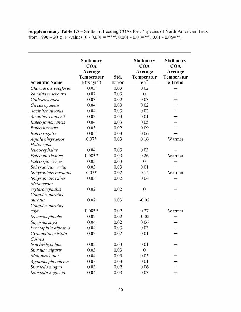
45

Supplementary Table 1.7 – Shifts in Breeding COAs for 77 species of North American Birds from 1990 – 2015. P -values (0 - 0.001 = '***', 0.001 - 0.01='**', 0.01 - 0.05='*').

Scientific Name

Stationary COA

Average Temperature (°C yr-1)

Std. Error

Stationary COA

Average Temperatur

e r2

Stationary COA

Average Temperatur

e Trend Charadrius vociferus 0.03 0.03 0.02 ─ Zenaida macroura 0.02 0.03 0 ─ Cathartes aura 0.03 0.02 0.03 ─ Circus cyaneus 0.04 0.03 0.02 ─ Accipiter striatus 0.04 0.03 0.02 ─ Accipiter cooperii 0.03 0.03 0.01 ─ Buteo jamaicensis 0.04 0.03 0.05 ─ Buteo lineatus 0.03 0.02 0.09 ─ Buteo regalis 0.05 0.03 0.06 ─ Aquila chrysaetos 0.07* 0.03 0.16 Warmer Haliaeetus leucocephalus 0.04 0.03 0.03 ─ Falco mexicanus 0.08** 0.03 0.26 Warmer Falco sparverius 0.03 0.03 0 ─ Sphyrapicus varius 0.03 0.03 0.01 ─ Sphyrapicus nuchalis 0.05* 0.02 0.15 Warmer Sphyrapicus ruber 0.03 0.02 0.04 ─ Melanerpes erythrocephalus 0.02 0.02 0 ─ Colaptes auratus auratus 0.02 0.03 -0.02 ─ Colaptes auratus cafer 0.08** 0.02 0.27 Warmer Sayornis phoebe 0.02 0.02 -0.02 ─ Sayornis saya 0.04 0.02 0.06 ─ Eremophila alpestris 0.04 0.03 0.03 ─ Cyanocitta cristata 0.03 0.02 0.01 ─ Corvus brachyrhynchos 0.03 0.03 0.01 ─ Sturnus vulgaris 0.03 0.03 0 ─ Molothrus ater 0.04 0.03 0.05 ─ Agelaius phoeniceus 0.03 0.03 0.01 ─ Sturnella magna 0.03 0.02 0.06 ─ Sturnella neglecta 0.04 0.03 0.03 ─

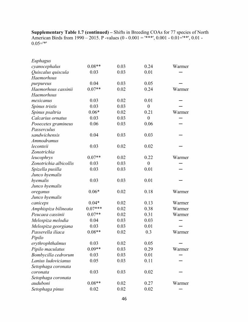
46

Supplementary Table 1.7 (continued) – Shifts in Breeding COAs for 77 species of North American Birds from 1990 – 2015. P -values (0 - 0.001 = '***', 0.001 - 0.01='**', 0.01 - 0.05='*' Euphagus cyanocephalus 0.08** 0.03 0.24 Warmer Quiscalus quiscula 0.03 0.03 0.01 ─ Haemorhous purpureus 0.04 0.03 0.05 ─ Haemorhous cassinii 0.07** 0.02 0.24 Warmer Haemorhous mexicanus 0.03 0.02 0.01 ─ Spinus tristis 0.03 0.03 0 ─ Spinus psaltria 0.06* 0.02 0.21 Warmer Calcarius ornatus 0.03 0.03 0 ─ Pooecetes gramineus 0.06 0.03 0.06 ─ Passerculus sandwichensis 0.04 0.03 0.03 ─ Ammodramus leconteii 0.03 0.02 0.02 ─ Zonotrichia leucophrys 0.07** 0.02 0.22 Warmer Zonotrichia albicollis 0.03 0.03 0 ─ Spizella pusilla 0.03 0.03 0.01 ─ Junco hyemalis hyemalis 0.03 0.03 0.01 ─ Junco hyemalis oreganus 0.06* 0.02 0.18 Warmer Junco hyemalis caniceps 0.04* 0.02 0.13 Warmer Amphispiza bilineata 0.07*** 0.02 0.38 Warmer Peucaea cassinii 0.07** 0.02 0.31 Warmer Melospiza melodia 0.04 0.03 0.03 ─ Melospiza georgiana 0.03 0.03 0.01 ─ Passerella iliaca 0.08** 0.02 0.3 Warmer Pipilo erythrophthalmus 0.03 0.02 0.05 ─ Pipilo maculatus 0.09** 0.03 0.29 Warmer Bombycilla cedrorum 0.03 0.03 0.01 ─ Lanius ludovicianus 0.05 0.03 0.11 ─ Setophaga coronata coronata 0.03 0.03 0.02 ─ Setophaga coronata auduboni 0.08** 0.02 0.27 Warmer Setophaga pinus 0.02 0.02 0.02 ─

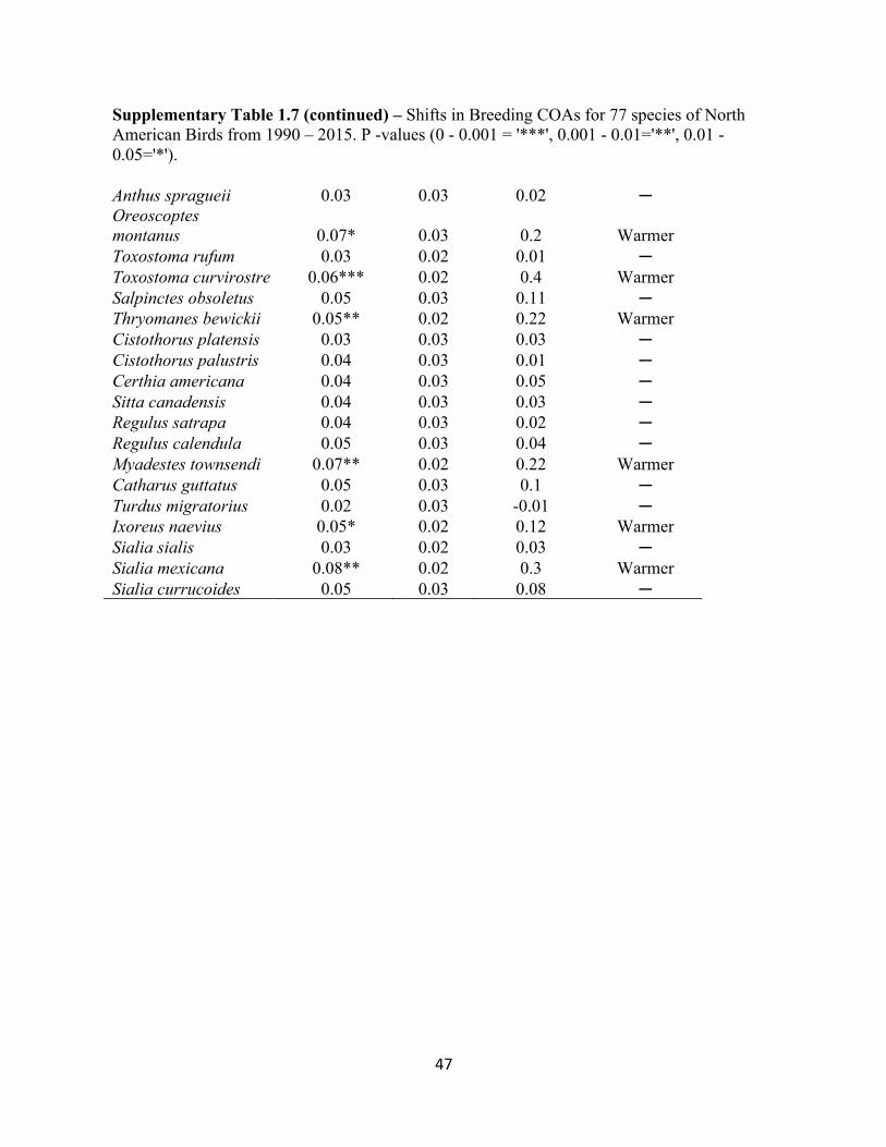
47

Supplementary Table 1.7 (continued) – Shifts in Breeding COAs for 77 species of North American Birds from 1990 – 2015. P -values (0 - 0.001 = '***', 0.001 - 0.01='**', 0.01 - 0.05='*'). Anthus spragueii 0.03 0.03 0.02 ─ Oreoscoptes montanus 0.07* 0.03 0.2 Warmer Toxostoma rufum 0.03 0.02 0.01 ─ Toxostoma curvirostre 0.06*** 0.02 0.4 Warmer Salpinctes obsoletus 0.05 0.03 0.11 ─ Thryomanes bewickii 0.05** 0.02 0.22 Warmer Cistothorus platensis 0.03 0.03 0.03 ─ Cistothorus palustris 0.04 0.03 0.01 ─ Certhia americana 0.04 0.03 0.05 ─ Sitta canadensis 0.04 0.03 0.03 ─ Regulus satrapa 0.04 0.03 0.02 ─ Regulus calendula 0.05 0.03 0.04 ─ Myadestes townsendi 0.07** 0.02 0.22 Warmer Catharus guttatus 0.05 0.03 0.1 ─ Turdus migratorius 0.02 0.03 -0.01 ─ Ixoreus naevius 0.05* 0.02 0.12 Warmer Sialia sialis 0.03 0.02 0.03 ─ Sialia mexicana 0.08** 0.02 0.3 Warmer Sialia currucoides 0.05 0.03 0.08 ─

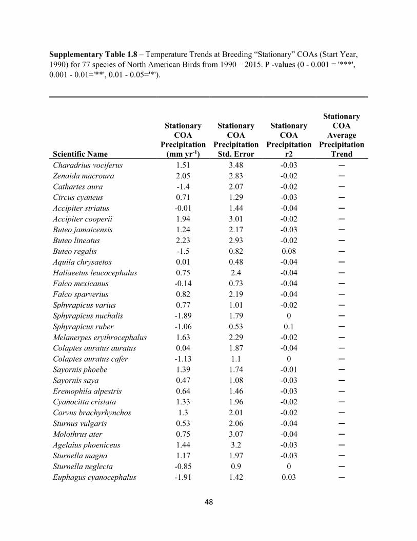
48

Supplementary Table 1.8 – Temperature Trends at Breeding “Stationary” COAs (Start Year, 1990) for 77 species of North American Birds from 1990 – 2015. P -values (0 - 0.001 = '***', 0.001 - 0.01='**', 0.01 - 0.05='*').

Scientific Name

Stationary COA

Precipitation (mm yr-1)

Stationary COA

Precipitation Std. Error

Stationary COA

Precipitation r2

Stationary COA

Average Precipitation

Trend Charadrius vociferus 1.51 3.48 -0.03 ─ Zenaida macroura 2.05 2.83 -0.02 ─ Cathartes aura -1.4 2.07 -0.02 ─ Circus cyaneus 0.71 1.29 -0.03 ─ Accipiter striatus -0.01 1.44 -0.04 ─ Accipiter cooperii 1.94 3.01 -0.02 ─ Buteo jamaicensis 1.24 2.17 -0.03 ─ Buteo lineatus 2.23 2.93 -0.02 ─ Buteo regalis -1.5 0.82 0.08 ─ Aquila chrysaetos 0.01 0.48 -0.04 ─ Haliaeetus leucocephalus 0.75 2.4 -0.04 ─ Falco mexicanus -0.14 0.73 -0.04 ─ Falco sparverius 0.82 2.19 -0.04 ─ Sphyrapicus varius 0.77 1.01 -0.02 ─ Sphyrapicus nuchalis -1.89 1.79 0 ─ Sphyrapicus ruber -1.06 0.53 0.1 ─ Melanerpes erythrocephalus 1.63 2.29 -0.02 ─ Colaptes auratus auratus 0.04 1.87 -0.04 ─ Colaptes auratus cafer -1.13 1.1 0 ─ Sayornis phoebe 1.39 1.74 -0.01 ─ Sayornis saya 0.47 1.08 -0.03 ─ Eremophila alpestris 0.64 1.46 -0.03 ─ Cyanocitta cristata 1.33 1.96 -0.02 ─ Corvus brachyrhynchos 1.3 2.01 -0.02 ─ Sturnus vulgaris 0.53 2.06 -0.04 ─ Molothrus ater 0.75 3.07 -0.04 ─ Agelaius phoeniceus 1.44 3.2 -0.03 ─ Sturnella magna 1.17 1.97 -0.03 ─ Sturnella neglecta -0.85 0.9 0 ─ Euphagus cyanocephalus -1.91 1.42 0.03 ─

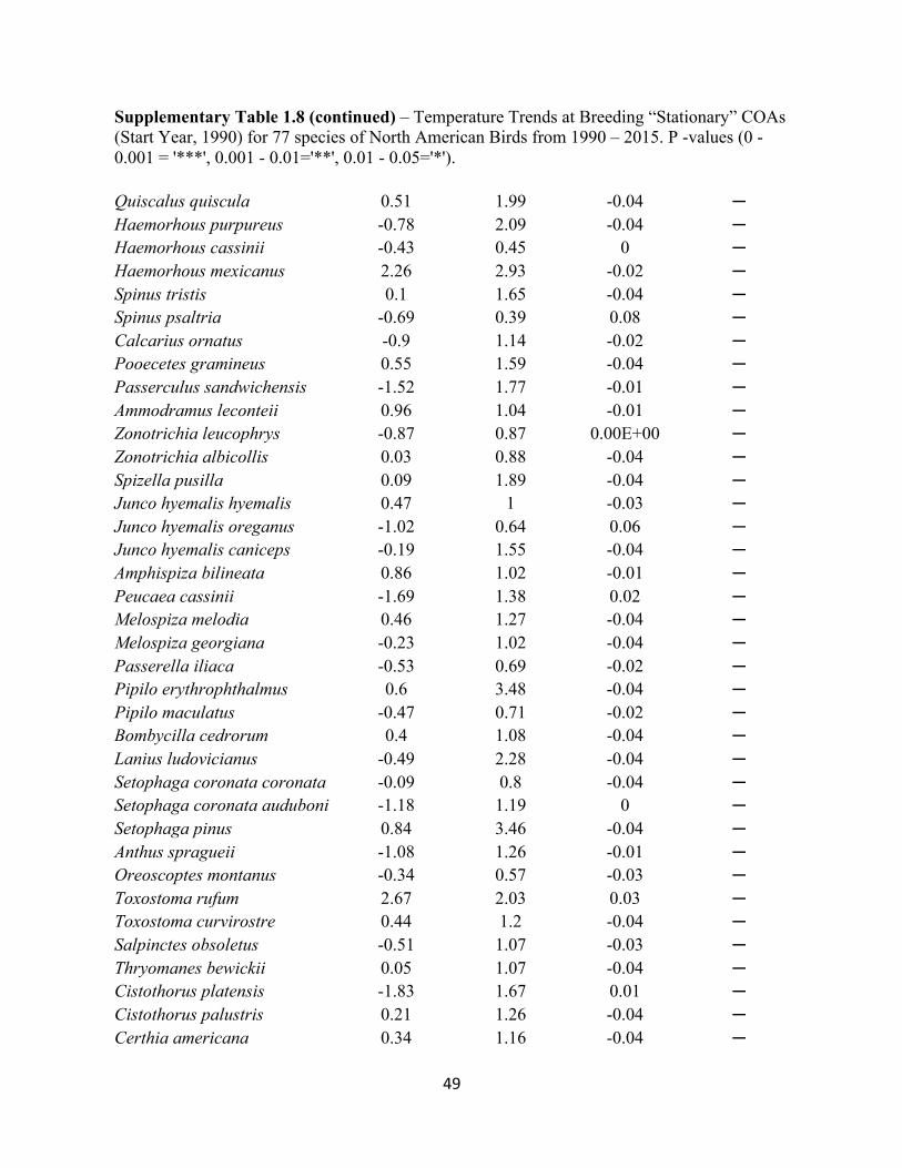
49

Supplementary Table 1.8 (continued) – Temperature Trends at Breeding “Stationary” COAs (Start Year, 1990) for 77 species of North American Birds from 1990 – 2015. P -values (0 - 0.001 = '***', 0.001 - 0.01='**', 0.01 - 0.05='*'). Quiscalus quiscula 0.51 1.99 -0.04 ─ Haemorhous purpureus -0.78 2.09 -0.04 ─ Haemorhous cassinii -0.43 0.45 0 ─ Haemorhous mexicanus 2.26 2.93 -0.02 ─ Spinus tristis 0.1 1.65 -0.04 ─ Spinus psaltria -0.69 0.39 0.08 ─ Calcarius ornatus -0.9 1.14 -0.02 ─ Pooecetes gramineus 0.55 1.59 -0.04 ─ Passerculus sandwichensis -1.52 1.77 -0.01 ─ Ammodramus leconteii 0.96 1.04 -0.01 ─ Zonotrichia leucophrys -0.87 0.87 0.00E+00 ─ Zonotrichia albicollis 0.03 0.88 -0.04 ─ Spizella pusilla 0.09 1.89 -0.04 ─ Junco hyemalis hyemalis 0.47 1 -0.03 ─ Junco hyemalis oreganus -1.02 0.64 0.06 ─ Junco hyemalis caniceps -0.19 1.55 -0.04 ─ Amphispiza bilineata 0.86 1.02 -0.01 ─ Peucaea cassinii -1.69 1.38 0.02 ─ Melospiza melodia 0.46 1.27 -0.04 ─ Melospiza georgiana -0.23 1.02 -0.04 ─ Passerella iliaca -0.53 0.69 -0.02 ─ Pipilo erythrophthalmus 0.6 3.48 -0.04 ─ Pipilo maculatus -0.47 0.71 -0.02 ─ Bombycilla cedrorum 0.4 1.08 -0.04 ─ Lanius ludovicianus -0.49 2.28 -0.04 ─ Setophaga coronata coronata -0.09 0.8 -0.04 ─ Setophaga coronata auduboni -1.18 1.19 0 ─ Setophaga pinus 0.84 3.46 -0.04 ─ Anthus spragueii -1.08 1.26 -0.01 ─ Oreoscoptes montanus -0.34 0.57 -0.03 ─ Toxostoma rufum 2.67 2.03 0.03 ─ Toxostoma curvirostre 0.44 1.2 -0.04 ─ Salpinctes obsoletus -0.51 1.07 -0.03 ─ Thryomanes bewickii 0.05 1.07 -0.04 ─ Cistothorus platensis -1.83 1.67 0.01 ─ Cistothorus palustris 0.21 1.26 -0.04 ─ Certhia americana 0.34 1.16 -0.04 ─

50

Supplementary Table 1.8 (continued) – Temperature Trends at Breeding “Stationary” COAs (Start Year, 1990) for 77 species of North American Birds from 1990 – 2015. P -values (0 - 0.001 = '***', 0.001 - 0.01='**', 0.01 - 0.05='*'). Sitta canadensis -0.49 1.11 -0.03 ─ Regulus satrapa -1.35 1.19 0.01 ─ Regulus calendula 0.53 1.29 -0.03 ─ Myadestes townsendi -0.47 0.74 -0.02 ─ Catharus guttatus -2.81 2.27 0.02 ─ Turdus migratorius 0.34 2.57 -0.04 ─ Ixoreus naevius -1.49* 0.55 0.2 Drier Sialia sialis 3.16 1.76 0.08 ─ Sialia mexicana -0.08 0.53 -0.04 ─ Sialia currucoides -1.36 1.44 0 ─

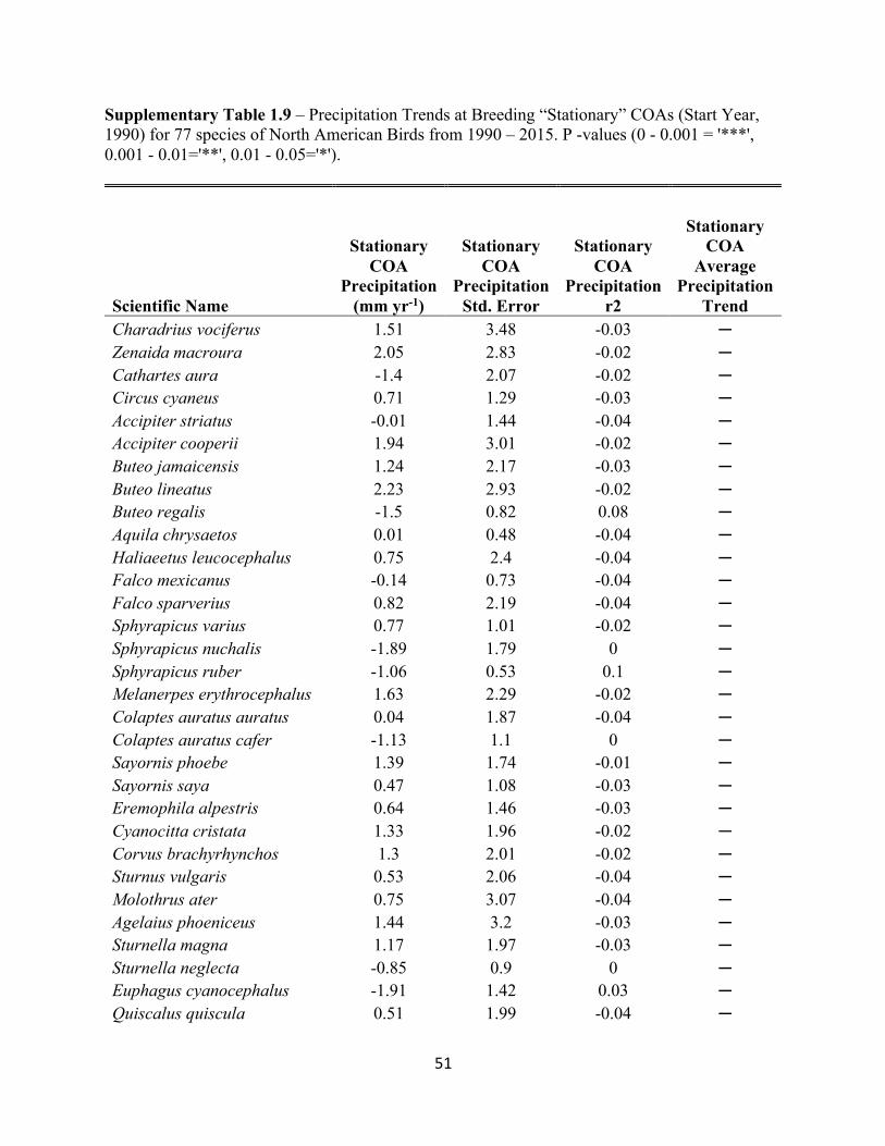
51

Supplementary Table 1.9 – Precipitation Trends at Breeding “Stationary” COAs (Start Year, 1990) for 77 species of North American Birds from 1990 – 2015. P -values (0 - 0.001 = '***', 0.001 - 0.01='**', 0.01 - 0.05='*').

Scientific Name

Stationary COA

Precipitation (mm yr-1)

Stationary COA

Precipitation Std. Error

Stationary COA

Precipitation r2

Stationary COA

Average Precipitation

Trend Charadrius vociferus 1.51 3.48 -0.03 ─ Zenaida macroura 2.05 2.83 -0.02 ─ Cathartes aura -1.4 2.07 -0.02 ─ Circus cyaneus 0.71 1.29 -0.03 ─ Accipiter striatus -0.01 1.44 -0.04 ─ Accipiter cooperii 1.94 3.01 -0.02 ─ Buteo jamaicensis 1.24 2.17 -0.03 ─ Buteo lineatus 2.23 2.93 -0.02 ─ Buteo regalis -1.5 0.82 0.08 ─ Aquila chrysaetos 0.01 0.48 -0.04 ─ Haliaeetus leucocephalus 0.75 2.4 -0.04 ─ Falco mexicanus -0.14 0.73 -0.04 ─ Falco sparverius 0.82 2.19 -0.04 ─ Sphyrapicus varius 0.77 1.01 -0.02 ─ Sphyrapicus nuchalis -1.89 1.79 0 ─ Sphyrapicus ruber -1.06 0.53 0.1 ─ Melanerpes erythrocephalus 1.63 2.29 -0.02 ─ Colaptes auratus auratus 0.04 1.87 -0.04 ─ Colaptes auratus cafer -1.13 1.1 0 ─ Sayornis phoebe 1.39 1.74 -0.01 ─ Sayornis saya 0.47 1.08 -0.03 ─ Eremophila alpestris 0.64 1.46 -0.03 ─ Cyanocitta cristata 1.33 1.96 -0.02 ─ Corvus brachyrhynchos 1.3 2.01 -0.02 ─ Sturnus vulgaris 0.53 2.06 -0.04 ─ Molothrus ater 0.75 3.07 -0.04 ─ Agelaius phoeniceus 1.44 3.2 -0.03 ─ Sturnella magna 1.17 1.97 -0.03 ─ Sturnella neglecta -0.85 0.9 0 ─ Euphagus cyanocephalus -1.91 1.42 0.03 ─ Quiscalus quiscula 0.51 1.99 -0.04 ─

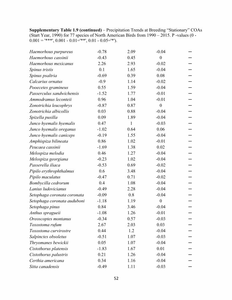
52

Supplementary Table 1.9 (continued) – Precipitation Trends at Breeding “Stationary” COAs (Start Year, 1990) for 77 species of North American Birds from 1990 – 2015. P -values (0 - 0.001 = '***', 0.001 - 0.01='**', 0.01 - 0.05='*'). Haemorhous purpureus -0.78 2.09 -0.04 ─ Haemorhous cassinii -0.43 0.45 0 ─ Haemorhous mexicanus 2.26 2.93 -0.02 ─ Spinus tristis 0.1 1.65 -0.04 ─ Spinus psaltria -0.69 0.39 0.08 ─ Calcarius ornatus -0.9 1.14 -0.02 ─ Pooecetes gramineus 0.55 1.59 -0.04 ─ Passerculus sandwichensis -1.52 1.77 -0.01 ─ Ammodramus leconteii 0.96 1.04 -0.01 ─ Zonotrichia leucophrys -0.87 0.87 0 ─ Zonotrichia albicollis 0.03 0.88 -0.04 ─ Spizella pusilla 0.09 1.89 -0.04 ─ Junco hyemalis hyemalis 0.47 1 -0.03 ─ Junco hyemalis oreganus -1.02 0.64 0.06 ─ Junco hyemalis caniceps -0.19 1.55 -0.04 ─ Amphispiza bilineata 0.86 1.02 -0.01 ─ Peucaea cassinii -1.69 1.38 0.02 ─ Melospiza melodia 0.46 1.27 -0.04 ─ Melospiza georgiana -0.23 1.02 -0.04 ─ Passerella iliaca -0.53 0.69 -0.02 ─ Pipilo erythrophthalmus 0.6 3.48 -0.04 ─ Pipilo maculatus -0.47 0.71 -0.02 ─ Bombycilla cedrorum 0.4 1.08 -0.04 ─ Lanius ludovicianus -0.49 2.28 -0.04 ─ Setophaga coronata coronata -0.09 0.8 -0.04 ─ Setophaga coronata auduboni -1.18 1.19 0 ─ Setophaga pinus 0.84 3.46 -0.04 ─ Anthus spragueii -1.08 1.26 -0.01 ─ Oreoscoptes montanus -0.34 0.57 -0.03 ─ Toxostoma rufum 2.67 2.03 0.03 ─ Toxostoma curvirostre 0.44 1.2 -0.04 ─ Salpinctes obsoletus -0.51 1.07 -0.03 ─ Thryomanes bewickii 0.05 1.07 -0.04 ─ Cistothorus platensis -1.83 1.67 0.01 ─ Cistothorus palustris 0.21 1.26 -0.04 ─ Certhia americana 0.34 1.16 -0.04 ─ Sitta canadensis -0.49 1.11 -0.03 ─

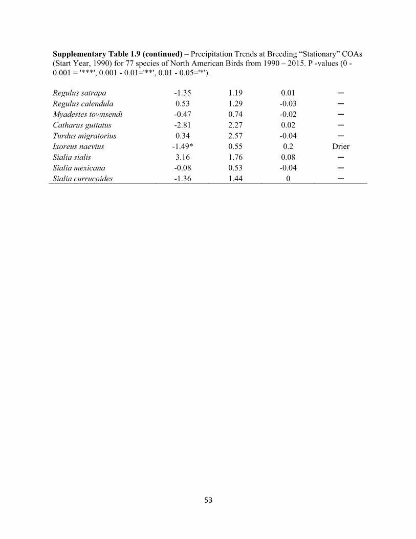
53

Supplementary Table 1.9 (continued) – Precipitation Trends at Breeding “Stationary” COAs (Start Year, 1990) for 77 species of North American Birds from 1990 – 2015. P -values (0 - 0.001 = '***', 0.001 - 0.01='**', 0.01 - 0.05='*'). Regulus satrapa -1.35 1.19 0.01 ─ Regulus calendula 0.53 1.29 -0.03 ─ Myadestes townsendi -0.47 0.74 -0.02 ─ Catharus guttatus -2.81 2.27 0.02 ─ Turdus migratorius 0.34 2.57 -0.04 ─ Ixoreus naevius -1.49* 0.55 0.2 Drier Sialia sialis 3.16 1.76 0.08 ─ Sialia mexicana -0.08 0.53 -0.04 ─ Sialia currucoides -1.36 1.44 0 ─

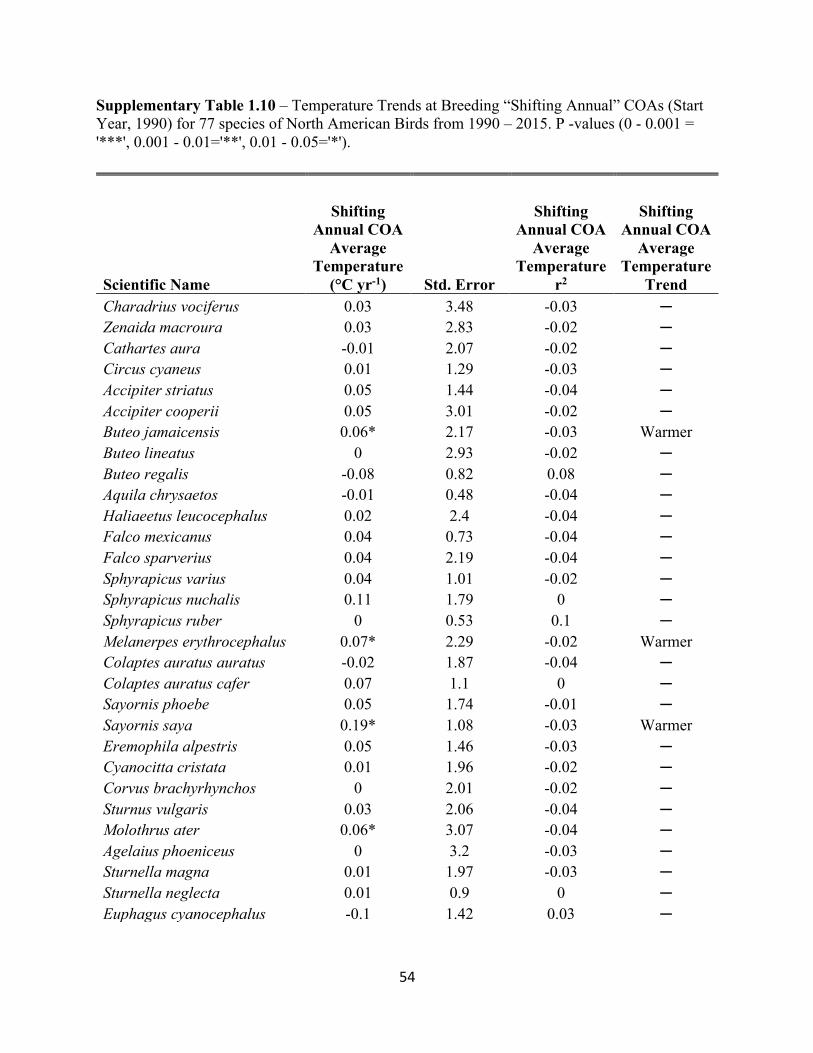
54

Supplementary Table 1.10 – Temperature Trends at Breeding “Shifting Annual” COAs (Start Year, 1990) for 77 species of North American Birds from 1990 – 2015. P -values (0 - 0.001 = '***', 0.001 - 0.01='**', 0.01 - 0.05='*').

Scientific Name

Shifting Annual COA

Average Temperature

(°C yr-1) Std. Error

Shifting Annual COA

Average Temperature

r2

Shifting Annual COA

Average Temperature

Trend Charadrius vociferus 0.03 3.48 -0.03 ─ Zenaida macroura 0.03 2.83 -0.02 ─ Cathartes aura -0.01 2.07 -0.02 ─ Circus cyaneus 0.01 1.29 -0.03 ─ Accipiter striatus 0.05 1.44 -0.04 ─ Accipiter cooperii 0.05 3.01 -0.02 ─ Buteo jamaicensis 0.06* 2.17 -0.03 Warmer Buteo lineatus 0 2.93 -0.02 ─ Buteo regalis -0.08 0.82 0.08 ─ Aquila chrysaetos -0.01 0.48 -0.04 ─ Haliaeetus leucocephalus 0.02 2.4 -0.04 ─ Falco mexicanus 0.04 0.73 -0.04 ─ Falco sparverius 0.04 2.19 -0.04 ─ Sphyrapicus varius 0.04 1.01 -0.02 ─ Sphyrapicus nuchalis 0.11 1.79 0 ─ Sphyrapicus ruber 0 0.53 0.1 ─ Melanerpes erythrocephalus 0.07* 2.29 -0.02 Warmer Colaptes auratus auratus -0.02 1.87 -0.04 ─ Colaptes auratus cafer 0.07 1.1 0 ─ Sayornis phoebe 0.05 1.74 -0.01 ─ Sayornis saya 0.19* 1.08 -0.03 Warmer Eremophila alpestris 0.05 1.46 -0.03 ─ Cyanocitta cristata 0.01 1.96 -0.02 ─ Corvus brachyrhynchos 0 2.01 -0.02 ─ Sturnus vulgaris 0.03 2.06 -0.04 ─ Molothrus ater 0.06* 3.07 -0.04 ─ Agelaius phoeniceus 0 3.2 -0.03 ─ Sturnella magna 0.01 1.97 -0.03 ─ Sturnella neglecta 0.01 0.9 0 ─ Euphagus cyanocephalus -0.1 1.42 0.03 ─

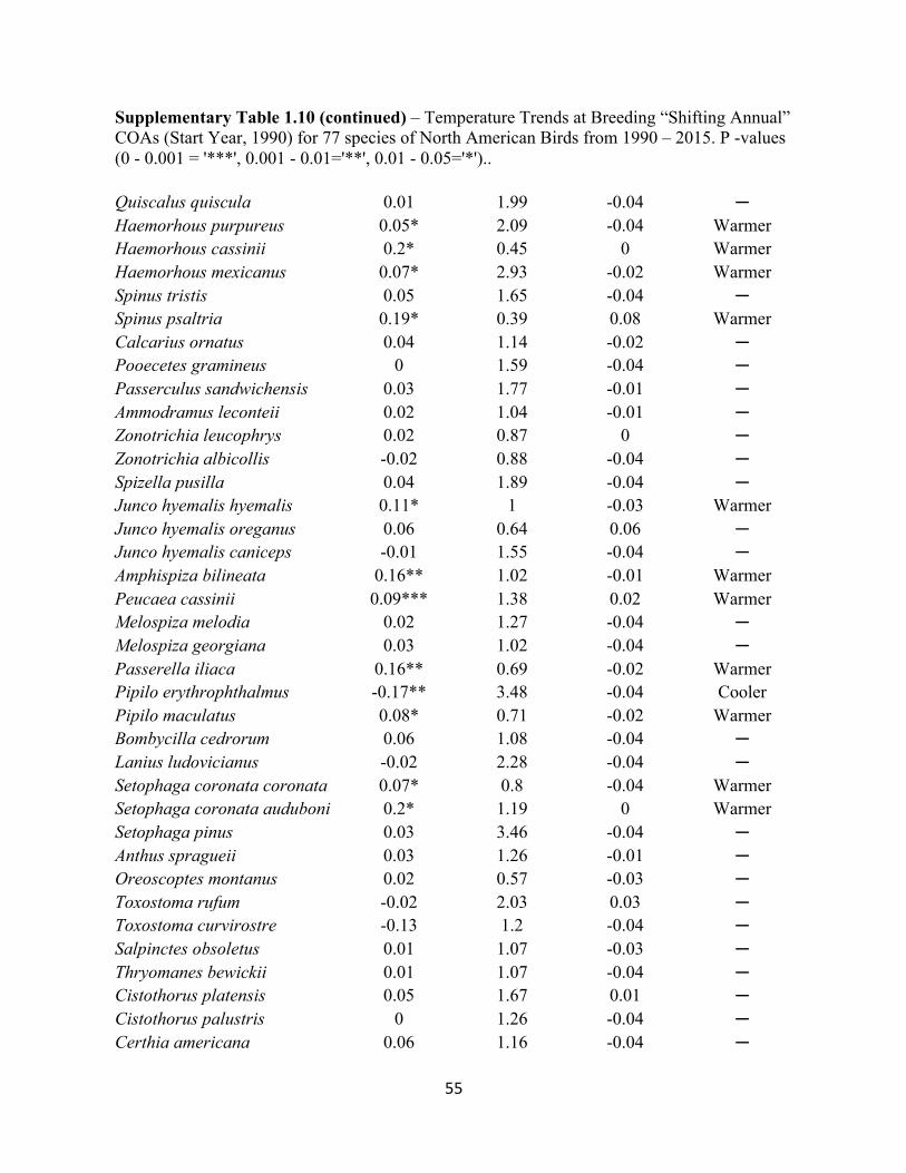
55

Supplementary Table 1.10 (continued) – Temperature Trends at Breeding “Shifting Annual” COAs (Start Year, 1990) for 77 species of North American Birds from 1990 – 2015. P -values (0 - 0.001 = '***', 0.001 - 0.01='**', 0.01 - 0.05='*').. Quiscalus quiscula 0.01 1.99 -0.04 ─ Haemorhous purpureus 0.05* 2.09 -0.04 Warmer Haemorhous cassinii 0.2* 0.45 0 Warmer Haemorhous mexicanus 0.07* 2.93 -0.02 Warmer Spinus tristis 0.05 1.65 -0.04 ─ Spinus psaltria 0.19* 0.39 0.08 Warmer Calcarius ornatus 0.04 1.14 -0.02 ─ Pooecetes gramineus 0 1.59 -0.04 ─ Passerculus sandwichensis 0.03 1.77 -0.01 ─ Ammodramus leconteii 0.02 1.04 -0.01 ─ Zonotrichia leucophrys 0.02 0.87 0 ─ Zonotrichia albicollis -0.02 0.88 -0.04 ─ Spizella pusilla 0.04 1.89 -0.04 ─ Junco hyemalis hyemalis 0.11* 1 -0.03 Warmer Junco hyemalis oreganus 0.06 0.64 0.06 ─ Junco hyemalis caniceps -0.01 1.55 -0.04 ─ Amphispiza bilineata 0.16** 1.02 -0.01 Warmer Peucaea cassinii 0.09*** 1.38 0.02 Warmer Melospiza melodia 0.02 1.27 -0.04 ─ Melospiza georgiana 0.03 1.02 -0.04 ─ Passerella iliaca 0.16** 0.69 -0.02 Warmer Pipilo erythrophthalmus -0.17** 3.48 -0.04 Cooler Pipilo maculatus 0.08* 0.71 -0.02 Warmer Bombycilla cedrorum 0.06 1.08 -0.04 ─ Lanius ludovicianus -0.02 2.28 -0.04 ─ Setophaga coronata coronata 0.07* 0.8 -0.04 Warmer Setophaga coronata auduboni 0.2* 1.19 0 Warmer Setophaga pinus 0.03 3.46 -0.04 ─ Anthus spragueii 0.03 1.26 -0.01 ─ Oreoscoptes montanus 0.02 0.57 -0.03 ─ Toxostoma rufum -0.02 2.03 0.03 ─ Toxostoma curvirostre -0.13 1.2 -0.04 ─ Salpinctes obsoletus 0.01 1.07 -0.03 ─ Thryomanes bewickii 0.01 1.07 -0.04 ─ Cistothorus platensis 0.05 1.67 0.01 ─ Cistothorus palustris 0 1.26 -0.04 ─ Certhia americana 0.06 1.16 -0.04 ─

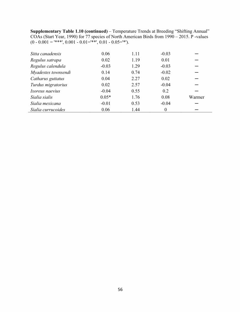
56

Supplementary Table 1.10 (continued) – Temperature Trends at Breeding “Shifting Annual” COAs (Start Year, 1990) for 77 species of North American Birds from 1990 – 2015. P -values (0 - 0.001 = '***', 0.001 - 0.01='**', 0.01 - 0.05='*'). Sitta canadensis 0.06 1.11 -0.03 ─ Regulus satrapa 0.02 1.19 0.01 ─ Regulus calendula -0.03 1.29 -0.03 ─ Myadestes townsendi 0.14 0.74 -0.02 ─ Catharus guttatus 0.04 2.27 0.02 ─ Turdus migratorius 0.02 2.57 -0.04 ─ Ixoreus naevius -0.04 0.55 0.2 ─ Sialia sialis 0.05* 1.76 0.08 Warmer Sialia mexicana -0.01 0.53 -0.04 ─ Sialia currucoides 0.06 1.44 0 ─

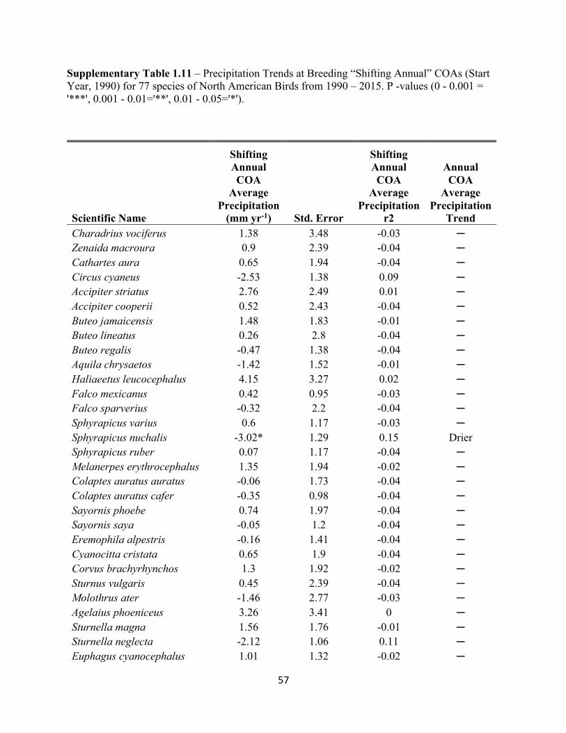
57

Supplementary Table 1.11 – Precipitation Trends at Breeding “Shifting Annual” COAs (Start Year, 1990) for 77 species of North American Birds from 1990 – 2015. P -values (0 - 0.001 = '***', 0.001 - 0.01='**', 0.01 - 0.05='*').

Scientific Name

Shifting Annual COA

Average Precipitation

(mm yr-1) Std. Error

Shifting Annual COA

Average Precipitation

r2

Annual COA

Average Precipitation

Trend Charadrius vociferus 1.38 3.48 -0.03 ─ Zenaida macroura 0.9 2.39 -0.04 ─ Cathartes aura 0.65 1.94 -0.04 ─ Circus cyaneus -2.53 1.38 0.09 ─ Accipiter striatus 2.76 2.49 0.01 ─ Accipiter cooperii 0.52 2.43 -0.04 ─ Buteo jamaicensis 1.48 1.83 -0.01 ─ Buteo lineatus 0.26 2.8 -0.04 ─ Buteo regalis -0.47 1.38 -0.04 ─ Aquila chrysaetos -1.42 1.52 -0.01 ─ Haliaeetus leucocephalus 4.15 3.27 0.02 ─ Falco mexicanus 0.42 0.95 -0.03 ─ Falco sparverius -0.32 2.2 -0.04 ─ Sphyrapicus varius 0.6 1.17 -0.03 ─ Sphyrapicus nuchalis -3.02* 1.29 0.15 Drier Sphyrapicus ruber 0.07 1.17 -0.04 ─ Melanerpes erythrocephalus 1.35 1.94 -0.02 ─ Colaptes auratus auratus -0.06 1.73 -0.04 ─ Colaptes auratus cafer -0.35 0.98 -0.04 ─ Sayornis phoebe 0.74 1.97 -0.04 ─ Sayornis saya -0.05 1.2 -0.04 ─ Eremophila alpestris -0.16 1.41 -0.04 ─ Cyanocitta cristata 0.65 1.9 -0.04 ─ Corvus brachyrhynchos 1.3 1.92 -0.02 ─ Sturnus vulgaris 0.45 2.39 -0.04 ─ Molothrus ater -1.46 2.77 -0.03 ─ Agelaius phoeniceus 3.26 3.41 0 ─ Sturnella magna 1.56 1.76 -0.01 ─ Sturnella neglecta -2.12 1.06 0.11 ─ Euphagus cyanocephalus 1.01 1.32 -0.02 ─

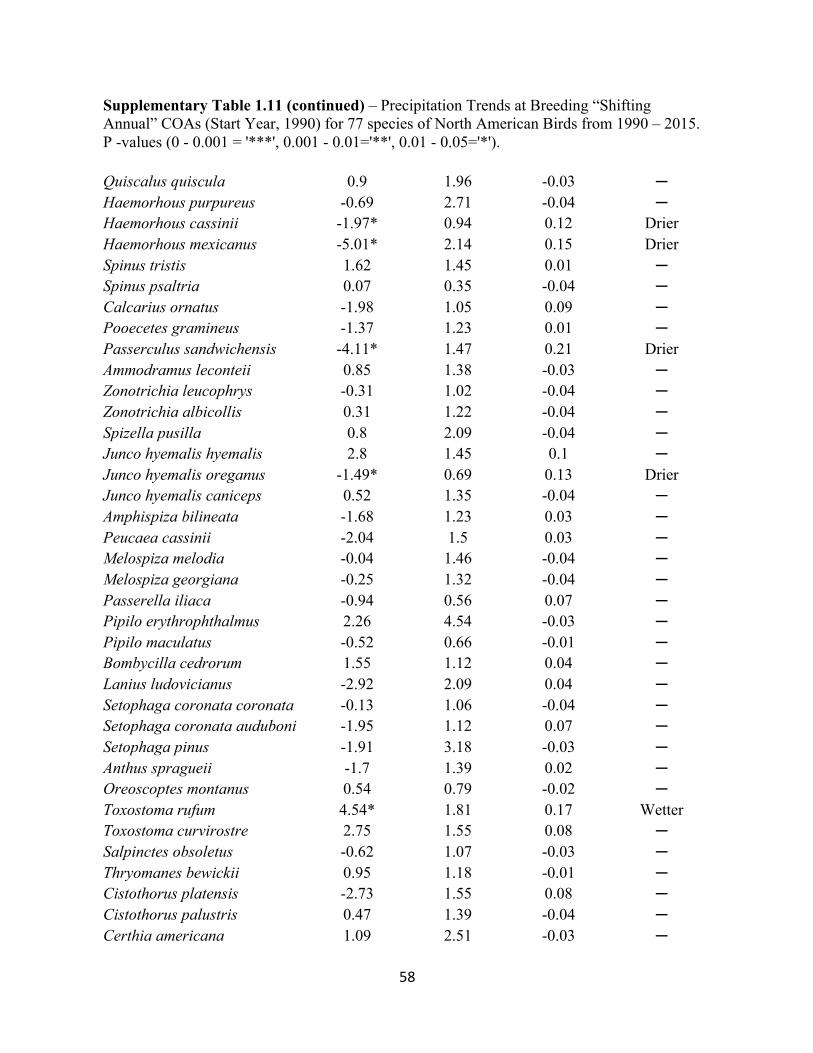
58

Supplementary Table 1.11 (continued) – Precipitation Trends at Breeding “Shifting Annual” COAs (Start Year, 1990) for 77 species of North American Birds from 1990 – 2015. P -values (0 - 0.001 = '***', 0.001 - 0.01='**', 0.01 - 0.05='*'). Quiscalus quiscula 0.9 1.96 -0.03 ─ Haemorhous purpureus -0.69 2.71 -0.04 ─ Haemorhous cassinii -1.97* 0.94 0.12 Drier Haemorhous mexicanus -5.01* 2.14 0.15 Drier Spinus tristis 1.62 1.45 0.01 ─ Spinus psaltria 0.07 0.35 -0.04 ─ Calcarius ornatus -1.98 1.05 0.09 ─ Pooecetes gramineus -1.37 1.23 0.01 ─ Passerculus sandwichensis -4.11* 1.47 0.21 Drier Ammodramus leconteii 0.85 1.38 -0.03 ─ Zonotrichia leucophrys -0.31 1.02 -0.04 ─ Zonotrichia albicollis 0.31 1.22 -0.04 ─ Spizella pusilla 0.8 2.09 -0.04 ─ Junco hyemalis hyemalis 2.8 1.45 0.1 ─ Junco hyemalis oreganus -1.49* 0.69 0.13 Drier Junco hyemalis caniceps 0.52 1.35 -0.04 ─ Amphispiza bilineata -1.68 1.23 0.03 ─ Peucaea cassinii -2.04 1.5 0.03 ─ Melospiza melodia -0.04 1.46 -0.04 ─ Melospiza georgiana -0.25 1.32 -0.04 ─ Passerella iliaca -0.94 0.56 0.07 ─ Pipilo erythrophthalmus 2.26 4.54 -0.03 ─ Pipilo maculatus -0.52 0.66 -0.01 ─ Bombycilla cedrorum 1.55 1.12 0.04 ─ Lanius ludovicianus -2.92 2.09 0.04 ─ Setophaga coronata coronata -0.13 1.06 -0.04 ─ Setophaga coronata auduboni -1.95 1.12 0.07 ─ Setophaga pinus -1.91 3.18 -0.03 ─ Anthus spragueii -1.7 1.39 0.02 ─ Oreoscoptes montanus 0.54 0.79 -0.02 ─ Toxostoma rufum 4.54* 1.81 0.17 Wetter Toxostoma curvirostre 2.75 1.55 0.08 ─ Salpinctes obsoletus -0.62 1.07 -0.03 ─ Thryomanes bewickii 0.95 1.18 -0.01 ─ Cistothorus platensis -2.73 1.55 0.08 ─ Cistothorus palustris 0.47 1.39 -0.04 ─ Certhia americana 1.09 2.51 -0.03 ─

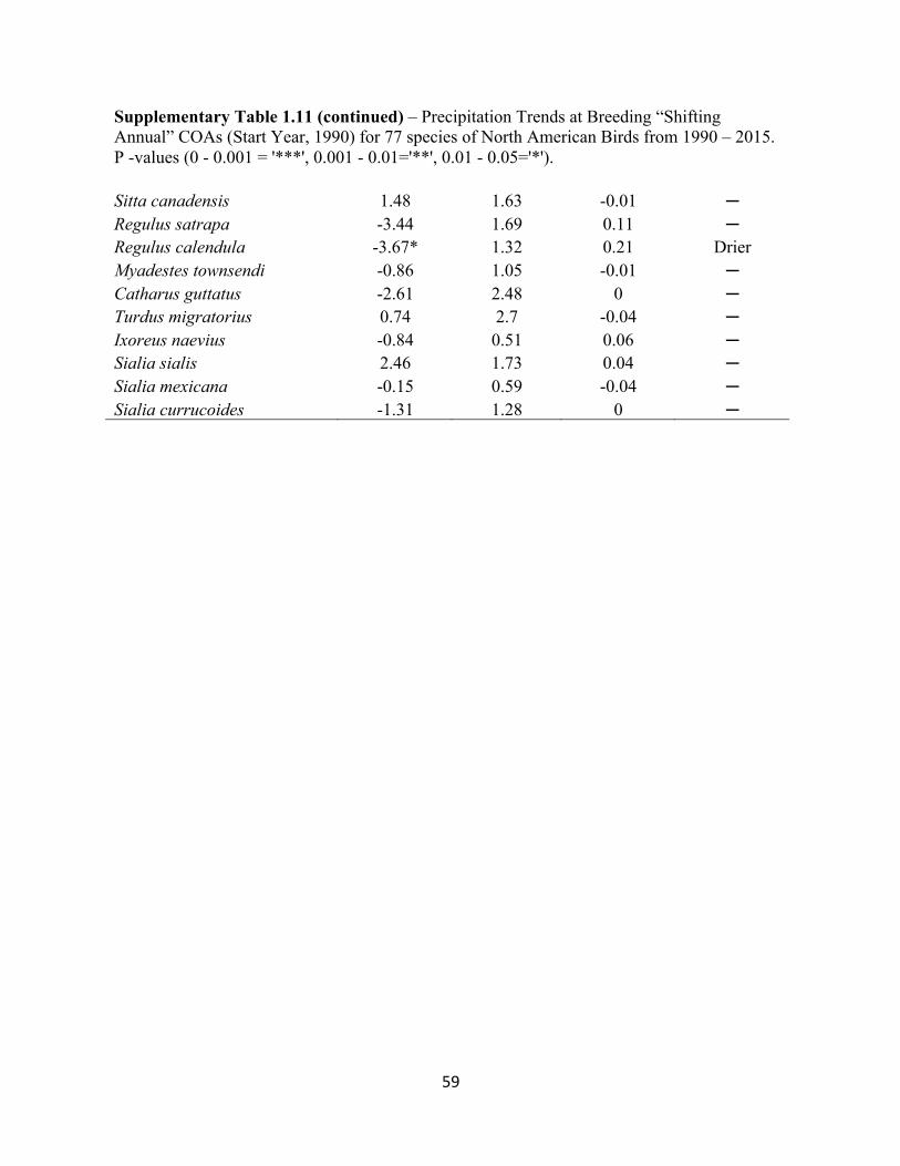
59

Supplementary Table 1.11 (continued) – Precipitation Trends at Breeding “Shifting Annual” COAs (Start Year, 1990) for 77 species of North American Birds from 1990 – 2015. P -values (0 - 0.001 = '***', 0.001 - 0.01='**', 0.01 - 0.05='*'). Sitta canadensis 1.48 1.63 -0.01 ─ Regulus satrapa -3.44 1.69 0.11 ─ Regulus calendula -3.67* 1.32 0.21 Drier Myadestes townsendi -0.86 1.05 -0.01 ─ Catharus guttatus -2.61 2.48 0 ─ Turdus migratorius 0.74 2.7 -0.04 ─ Ixoreus naevius -0.84 0.51 0.06 ─ Sialia sialis 2.46 1.73 0.04 ─ Sialia mexicana -0.15 0.59 -0.04 ─ Sialia currucoides -1.31 1.28 0 ─

60

Chapter 2

Changes in community temperature & precipitation indices over time and space reveal changing characteristics of ecological communities

2.1 ABSTRACT

Species distributions are becoming increasingly altered by changes in the earth’s climate.

Different responses by different species to climate can reshuffle communities, leading to complex

and unexpected changes. We used two community indices to investigate compositional changes,

the Community Temperature Index (CTI), which measures contributions of “warm” or “cool”

dwelling species in a community and a newly derived Community Precipitation Index (CPI),

which measures contributions of “high precipitation” or “low precipitation” tolerant species.

We hypothesized that CTI and CPI would each increase over time, due to increased abundances

of southernly distributed “warm” and “wet” increasing within communities. We used North

American Breeding Bird Survey (BBS) data from 1990 – 2017 from eastern North America. We

modeled spatiotemporal changes in CTI and CPI at the regional scale (all BBS sites) and a local

scale (BBS sites partitioned by 5° latitude bands), using Generalized Liner Mixed Models

(GLMMs). We then performed a jackknife analysis to determine the contribution of species to the

temporal trends of CTI and CPI. We used generalized linear models (GLMs) to ask if abundance

trends, habitat associations, or a species affinity for “warm /cool” and “high precipitation/low

precipitation” climates, contributed to the positive percent changes from the jackknifed models.

CTI and CPI both linearly increased at the regional scale due to increased abundances of “warm

dwelling” and “high precipitation tolerant” species. These trends were more variable at different

61

latitude bands. Individual species contributions to these temporal changes also varied with

latitude. At higher latitudes, we observed increased of abundances of southerly distributed

“warm / high precipitation” species and increased abundances of “low precipitation” species at

lower latitudes. We concluded the species decoupling between these indices support that

community composition had changed with respect to temperate and precipitation in breeding bird

communities over the last 28 years.

2.2 INTRODUCTION

As species distributions become increasingly altered by climate change, community

structure and function will also change (Morecroft & Speakman 2013). Pole-ward shifts and shifts

to higher elevations have been documented as a response to increasingly warm temperatures

(Thomas & Lennon 1999, Parmesan & Yohe 2003, Hickling et al. 2006, Tingley et al. 2012).

However, meta-analyses show a diversity of responses across different regions and taxa (Chen et

al. 2011). The diversity of species responses indicates that temperature alone is not altering

community composition. Rather, competition and responses to precipitation changes have also

been shown to impact species distributions (Van Der Wall et al. 2013, Alexander et al. 2015).

In addition, climate change is not occurring uniformly across landscapes, therefore, identifying

geographic trends of community composition with temperature and precipitation changes is

important for formulating more effective responses to climate change (Savage et al. 2015).

Community indices have been used to quantify changes in species composition while

accounting for temporal changes in community characteristics. One such index is the

Community Temperature Index (CTI), which is a weighted ratio of “warmer” vs “cooler”

dwelling species within a community (Devictor et al. 2008, Devictor et al. 2012). It is calculated

from the average temperature of an individual species’ geographic range - a Species Temperature

62

Index (STI) - which reflects a thermal envelope of a species (Thuiller et al. 2005, Hijmans &

Graham 2006). This value is weighted by the abundance of each species within a community to

develop a CTI value (°C). Relatively lower CTI values represent communities composed of more

cool dwelling species. Temporal changes in CTI are used to evaluate how communities are

responding to climate change as species assemblages change. A Community Precipitation Index

(CPI) is similarly derived by using species’ average precipitation within its range (mm).

A positive linear relationship between CTI and time has been observed in several

communities (Devictor et al. 2008, 2012; Godet et al. 2011; Princé & Zuckerberg 2015) In eastern

North America, CTI increased in winter communities of birds, driven by increases of “warm-

dwelling” southern species shifting to higher latitudes (Princé & Zuckerberg 2015). However, this

study predominantly incorporated birds that frequent bird feeders and largely representing a single

feeding guild. Supplementary feeding of wintering birds logically influences northward range

expansion of more southerly-distributed species (Robb et al. 2008) which may inherently influence

results.

In summer, shifts in avian species distributions have been shown to be more variable in

comparison to those in winter (Huang et al. 2016, Currie & Venne 2017, Curley et al. in press),

and avian distributions do not always change in the direction and magnitude predicted by change

in temperature (Currie & Venne 2017, Curley et al. in press), which suggests that alternative

climate indices to CTI may be more useful for predicting changes in community composition.

In this study we use Breeding Bird Survey (BBS; US Geological Survey Patuxent

Wildlife Research Center, 2017) examine changes in community structure of eastern North

American birds from 1990-2015. We chose this time period and spatial scale to provide

comparable results to the similar study by Prince and Zuckerberg (2015). We test several

63

hypotheses: 1) that breeding bird communities are reflecting changes in climate and have a)

become increasingly composed of warm dwelling species (Wright et al. 1993, Hawkins et al. 2003)

and b) have become increasingly composed of species that are tolerant of higher levels of

precipitation. We used the previously established CTI and our newly derived CPI and analyzed

the spatiotemporal trends of these indices. We then examined how changes in these indices and

tested the hypothesis that CTI and CPI are predicted by species traits, habitat associations and

abundance trends.

2.3 METHODS

2.3.1 Breeding Bird Survey

We obtained data from The North American Breeding Bird Survey (BBS) from 1990-2017.

BBS is a network of annually sampled roadside surveys that are conducted during June to coincide

with the peak of the avian breeding season. Each route is 39.4 km long with 50, 3-minute point

counts spaced along the route. At each point count, all birds that are seen or heard within a 0.4 km

radius are recorded (US Geological Survey Patuxent Wildlife Research Center, 2015). We applied

a temporal filter to all BBS routes so that no routes missing 2 consecutive years of sampling were

included. We included 600 BBS routes in the eastern Unites States and Canada between -90° to -

60° longitude (East of the Mississippi River) and 25° to 50° latitude. Each BBS route was treated

as a single sample location (community) (Figure 2.1). We looked at BBS routes at a regional scale

(All BBS routes in the eastern United States) and at a local scale which consisted of 5° latitude

bands.

2.3.2 Species Selection and Classification

For the initial species pool, we followed the current taxonomy of North American birds

implemented by the American Ornithologists' Union (AOU; Chesser et al. 2018). To ensure only

64

well-sampled species were included in subsequent analyses, we selected species (from the

temporally filtered BBS routes), that occurred on at least 10 routes for each year of our study; 166

species met the criteria (supplementary material). The most recorded species was American Crow

(Corvus brachyrhynchos) with 15,439 individuals from 1990 to 2017. Least often recorded was

Willet (Tringa semipalmata) with 398 individuals recorded during our selected time window.

2.3.3 Species Temperature and Precipitation Indices

Seasonal temperature and precipitation variables were acquired from ClimateNA version

6.0 (Mitchell & Jones, 2005; http://tinyurl.com/ClimateNA.) Monthly temperature and

precipitation data are gridded at a 0.5 x 0.5° resolution. A species-specific temperature index (STI)

and precipitation index (SPI) were calculated from the average summer (May-June) temperature

(°C) and precipitation (mm) from occupancy data from BBS routes from 1970 to 1980 (Devictor

et al. 2008; Devictor et al. 2012). To remain consistent with location sampling, we included all

BBS routes throughout the United States and Canada that missed fewer than than 3 consecutive

years of surveying. STI ranged from 25.4⁰C to 14.03⁰C for Common Ground Dove (Columbia

passerine) and Magnolia Warbler (Setophaga magnolia) respectively. SPI ranged from 137.8mm

for White Ibis (Eudocimus albus) to 32.6mm for House Finch (Haemorhous mexicanus).

2.3.4 Community Temperature and Precipitation Indices (CTI/CPI)

From STI and SPI, we derived two functional indices of community composition, an annual

Community Temperature Index (CTI) and a Precipitation Index (CPI), each calculated from

weighted species abundances at each BBS location.

(1) !"#$ =∑ '(,*×,-.(,*/(01∑ '(,*/(01

(2) !3#$ =∑ '(,*×,4.(,*/(01∑ '(,*/(01

65

where ai,j is the abundance of species i at BBS route j, and n is the total number of species on that

route.

2.3.5 Modeling Spatiotemporal Trends in CTI and CPI

To model spatiotemporal changes in CTI and CPI, we used Generalized Linear Mixed

Models (GLMMs) with Year, Latitude and Longitude as fixed covariates (r package ‘nlme’;

Pinheiro et al. 2018). We included the BBS site as a random effect to account for the compound

correlation structure between BBS locations (Zuur 2009). Because we allowed intercepts to vary

between sites, we reduced the number of parameters included in our models (Zuur 2009).

2.3.6 Species Contribution to CTI and CPI – Jackknife

We implemented a Jackknife analysis (Crowley 1992, Davey et al. 2013, Princé &

Zuckerberg 2015, Tayleur et al. 2016) to assess individual species contribution to the

spatiotemporal trends in CTI and CPI. We iteratively removed species from the dataset and

recalculated the annual CTI and CPI for each BBS location. We then reran the GLMMs and

retained the new coefficient for our “Year” variable and calculated the percent difference between

the jackknifed model and original model coefficients (Davey et al. 2013, Princé & Zuckerberg

2015). Species with positive percent differences between the models positively contributed to the

temporal trends in CTI (CTIPD) and CPI (CPIPD). We repeated this process separately for each of

the 5 latitude bands.

2.3.7 Species contributions to changes in community indices

We used GLMs to access species contributions to the percent change of the global model,

using each species positive percent changes from jackknife models as the response. As predictor

variables, we accessed the abundance trends of each species via linear models against time and

retained the slope. Species abundances were then categorized as significantly increased, decreased

66

or unchanged over time. We then included the relative STI (STIREL) and SPI (SPIREL) of each

species by calculating the mean STI and SPI values from all 166 species in the pool. For example,

if a species’ STI or SPI fell above or below the mean of the species pool, the species was designated

“Warm / Cool” or “High Precipitation / Low Precipitation”. In addition to the abundance trend and

species STIREL-SPIREL combination, we included the primary habitat type of each species as a

categorical variable. These models were performed on the global data and repeated for each of the

latitude bands that had significant trends in CTI or CPI.

2.4 RESULTS

2.4.1 Temporal trends in CTI and CPI from the Global Model

From 1990 to 2017, in the eastern United States, CTI and CPI have significant temporal

trends (Figure 2.2a,b). CTI increased (1.58 ± 0.16× 10−3 °C yr−1, t-value = 9.85, P < 0.001) and

CPI increased (2.02 ± 0.13× 10−2 mm yr−1, t-value = 15.5, P < 0.001). The speed of northward

community shift occurred more rapidly in CPI than CTI (Figure 2.2). CTI had stronger shifts at

lower latitudes, whereas the rate of community shift was greater at higher latitudes for CPI.

2.4.2 Species Contributions to CTI and CPI from the Jackknife Global models

Species contributions to the spatiotemporal trends of CTI and CPI varied between species

and indices. Of the entire species pool, 79 of 166 species (47.6%) positively contributed to the CPI

trend and 75 species (45.2%) positively contributed to CPI. We report the 20 species whose

positive contributions to CPI and CTI were greatest (Table 2.1). For CTI, increasing “Warm/High

precipitation” species had the most positive affect on CTIPD (p = 0.0205). We found no significant

association between habitat type and CTIPD. For CPI, decreased “Warm / low precipitation”

species contributed to the positive percent values of CPI (p = 0.01). Species associated with Urban

habitats had the greatest positive relationship with CPIPD (p= 4.91e-08).

67

2.4.3 Temporal trends in CTI and CPI from the Latitude Bands

Changes in CTI and CPI were not consistent across the latitudinal bands. For Band 1, CTI

and CPI did not significantly change over time. CTI was significantly positive at bands 2-4 but

not at band 5 (Table 2.2). CPI was significantly negative at band 2, but significantly positive from

bands 3-5 (Figure 2.2). Overall, CTI had stronger shifts at lower latitudes, whereas the rate of

community shift was greater at higher latitudes for CPI.

2.4.4 Species Contributions to CTI and CPI from the Latitude Bands

Species contributions to CTI and CPI varied between the different latitude bands. Bands 2,

3 and 4 showed 46.3%, 50.6% and 48.4% of species with significant positive contributions to CTI.

For CPIPD, Band 2 had 55/135 species (41.0%) with a negative contribution to the negative trend

in CPI. Band 3 had 87/160 species (54.3%) with a positive CPIPD, Band 4 had 56/159 species

(40.8%) and Band 5 had 55/159 species (34.5%) with a positive CTIPD. We report the top 5 species

that had the highest CTIPD and CPIPD of each latitude band in Table 2.3.

GLM by Band–

Band 2 – For CTI, the decline of “Cool/High precipitation dwelling” species had the

greatest impact on the positive CTI trends (p = 0.027). Species associated with Open Woodlands

also showed the highest impacts on CTIPD (p = 0.045). For CPI, the decline of “Warm/High

precipitation” dwelling species had the biggest effect on the negative trend in CPI, particularly

species associated with Marsh habitat (p = 0.017)

Band 3 - For CTI, increase of “Warm temperature / High precipitation dwelling”

species affected the positive trend in CTI (p = 0.02832), attributed to species associated with

Open Woodlands (p = 0.00417). We found no significant habitat or trend variables for CPI at this

band.

68

Band 4 – We found no significant species trends or habitat associations at this band for

CTI. For CPI, species associated with Urban habitats showed the greatest contributions to CPIPD

(p = 0.2e-16 ). This was mainly due to the decline of one species, Haemorhous mexicanus (House

Finch). We ran the GLM for CPI after removing this species and found no significant habitat or

trend predictors at this band.

Band 5 – for CPI, there was significant relationship of increased abundance trend of

“Cool/High precipitation dwelling” species (p = 0.0274).

2.5 DISCUSSION

CTI and CPI increased in breeding bird communities across eastern North America from

1990-2015. Increased CTI was generally attributed to the northward shift of southerly distributed

species as a response to climate change and land use change (Kampichler et al. 2012, Princé &

Zuckerberg 2015). Our similarly derived CPI reflects community changes that result from

expected precipitation changes related to climate, and emphasizes the impact that changing

precipitation patterns will have on communities. Higher STI and SPIs were associated with

southern latitudes; therefore, changes in CTI/CPI are also appropriate in detecting more southernly

species shifting north; however, we found that different species contributed to each of the indices,

representing a decoupling between them.

CTI increased at a similar magnitude as in Devictor et al. 2008, Godet et al. 2011,

Lindström et al. 2013, Princé & Zuckerberg 2015. At the regional scale, the contributions of

increased “warm-dwelling” species are explained by northward range expansion of common,

generalist species. This finding and pattern is consistent with poleward shifts in species

distributions related to climate change and corroborates this as the mechanism which has already

been documented for winter avian communities (Prince and Zuckerberg) in eastern North America.

69

To our knowledge, this study is the first to assess avian community composition change

via a CPI index. Like CTI, CPI also increased at the regional scale, but interestingly, this

relationship did not hold true along the local latitudinal gradient. CPI significantly decreased

between 30°-35° but showed significant positive trends at the higher latitudes. It is possible that

community response to precipitation is more variable in comparison to temperature changes. This

presents an interesting avenue for further research. Broad-changes in precipitation patterns

occurred during the 20th century, with the subtropics and tropics becoming drier, and increased

precipitation at higher latitudes (Trenberth 2011). Avian species are known to follow their thermal

and precipitation niches (Tingley et al. 2009); therefore, we expect that at the community level,

CTI in conjunction with CPI to more accurately captures temporal changes of community

compositions.

In addition, community shifts occur at different rates between habitat types (Kampichler et

al. 2012), at different times of the year (Princé & Zuckerberg 2015), and along a latitudinal gradient

(Nieto-Sánchez et al. 2015, Magurran et al. 2015). We did not differentiate habitat types in this

study, but included the primary habitat in which a species occurred as an indicator of sensitivity to

community changes. From the global model, the greatest CTIPD contributions were attributed to

increasing trends of “warm/High precipitation dwelling” species. From the global model, habitat

type was not significant, but many species primarily associated with Forests and Open Woodlands

have positive CPIPD (Table 2.1). Of those species, many experienced northward range expansions

during the study period. This expansion may be due forest ecosystem changes in the eastern United

States over the study period (Nowacki & Abrams 2008, Fei et al. 2011). Our study did not focus

on land-use changes, but the northeastern United States has experienced reforestation with an

increase of secondary growth forests after an intense period of logging (Thompson et al. 2013),

70

which may create suitable habitat for forest-dwelling and open-woodland associated species. This

was not captured by our global / latitudinal band models, likely because the relative abundances

of forest-dwelling species were lower than urban-dwelling species at this resolution.

From the CPI global model, species associated with urban habitats showed the greatest

contributions. The species with the highest CPIPD was Haemorhous mexicanus (House Finch), a

widespread and common, “low precipitation” toloerant species, which experienced a steep

decrease in abundance during this time period (Table 2.1). A major contributor to their rapid

decline was the widespread outbreak of mycoplasmal conjunctivitis in the mid-Atlantic states,

resulting in ~60% population decline in its eastern population (Fischer et al. 1997; Hochachka &

Dhondt 2000; Dhondt et al. 2005). This is an extreme example of how a decline in species impacts

community indices without reflecting a change in climate.

Though species differentially impacted CTI and CPI, the two indices shared some

similarity in species that contributed to these changes. Species that positively contributed to CTIPD

CPIPD his model were common, southerly-distributed species which have expanded their ranges

northward, including Thryothorus ludovicianus (Carolina Wren), Cardinalis cardinalis (Northern

Cardinal) and Baeolophis bicolor (Tufted Titmouse), possibly driven by changes in distribution of

Forest ecosystems in the eastern United States (Nowacki & Abrams 2008, Fei et al. 2011), as

above.

Band 2 showed the most variability between CTI and CPI trends, with a positive trend in

CTI and a negative trend in CPI. We attributed the positive CTI increase to decreases in “cool”

dwelling species from this band, although no habitat significantly drove this shift. This indicates a

possible, more widespread phenomenon of species loss occurring at lower latitudes. Conversely,

we found a significantly negative slope of CPI at Band 2. Drastic increased abundances of “low

71

precipitation” affiliated species drove this negative relationship of CPI. The species that made the

most significant impact on this trend was Petrochelidon pyrrhonota (Cliff Swallow), a species

which nests in large colonies. In this study, they rapidly and steadily increased from 79 individuals

on 3 BBS routes in 1990 to over 500 individuals on 16 routes in 2017, a 545.5% increase in

abundance. This species expanded its breeding range into the southeastern United States, with new

colonies recorded every year (Brown et al. 2017). Rapid population declines of “High

precipitation-dwelling” species, such as Colinus virginianus (Northern Bobwhite), have also

contributed to this negative trend (Droege & Sauer 1990; Brennan 1991, Church et al. 1993,

Hernandez et al. 2013). Last, a widespread, “low precipitation” species, Zenaida macroura

(Mourning Dove), that has not experienced a significant abundance trend, also showed a large

CPIPD from the global model, indicating that the presence/absence of a species alone can cause

large deviations from a global model.

Our hypothesis that CTI and CPI would increase over time via southern “warm / wet –

dwelling” species moving north was supported by the Jackknife approach. This allowed us to

independently assess species contributions to the global model for both CTI and CPI, and make

comparisons between each species’ STIREL and SPIREL. For species that contributed positively to

both the CTI and CPI models, we found that many are “warm / wet” dwelling species that are

increasing in abundance. This is indicative of southern species expanding northward. However,

the jackknife approach also provided greater insight at the finer scale latitudinal bands; increases

in “low precipitation” species in the southern latitudes and decreases of “low precipitation” species

at the higher latitudes demonstrates that community changes are not occurring uniformly along a

latitudinal gradient. We concluded that multiple indices provide greater insight to how community

composition is changing over time.

72

Species in the eastern US clearly have responded to climate warming in such a way that

has translated to changes in the functional traits of communities. We have observed predictable

movement of species northward into the middle latitudinal bands, and expect that this trend will

continue over time if species continue to shift north with climate. We speculate that, since CPI is

has increased at this higher latitude band, that in the future, CTI will also increase. Band 2 has

opposing trends in CTI and CPI, we can infer from these results that CTI and CPI are changing at

different rates as species shift geographic ranges due to climate change: neither CTI nor CPI is

changing in band 1, CTI is still in flux in bands 2-4, and CPI is changing in bands 2-5 (Table 2.2).

We can speculate as to why we did not observe any changes band 1. Since a species pool was

already established prior to the study there was no way for new species to move into the lowest

latitude band from the Caribbean. This would have been the most logical way for CTI to increase

at this band. However, the failure to detect northward “cooler” dwelling species moving into the

lowest latitude band provides support that this system is primary being driven by southward

species expanding north.

The composition of breeding bird communities changed between 1990 and 2017. The

decoupling of our indices might be a useful tool in identifying which habitat types and which

species are more susceptible to climate and land use pressures (Kampichler et al. 2012). In

comparison to the winter bird communities examined by Prince and Zuckerberg (2015), our study

does not share many of the same species contributing to the positive trends in CTI. Our mechanism

of change, southern species shifting north, in similar to this previous study. This result suggests an

interesting dynamic about inter-seasonal community change via the same mechanism, with

different species contributing between seasons. In addition, our newly developed CPI revealed that

different species contribute to changes in temperature versus precipitation.

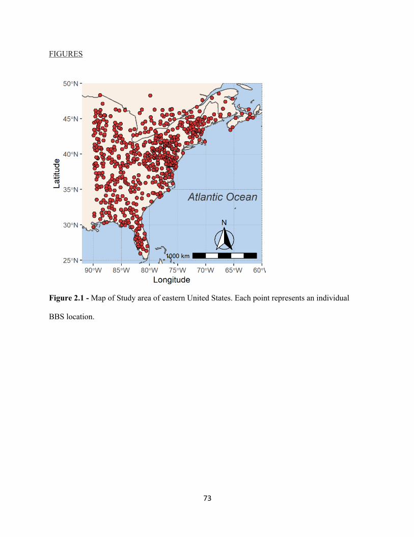
73

FIGURES

Figure 2.1 - Map of Study area of eastern United States. Each point represents an individual

BBS location.

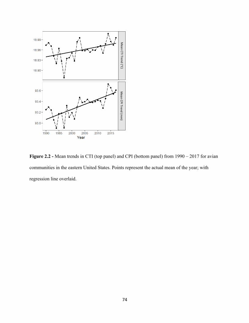
74

Figure 2.2 - Mean trends in CTI (top panel) and CPI (bottom panel) from 1990 – 2017 for avian

communities in the eastern United States. Points represent the actual mean of the year; with

regression line overlaid.

Mean CTI Trend (°C)

Mean CPI Trend (m

m)

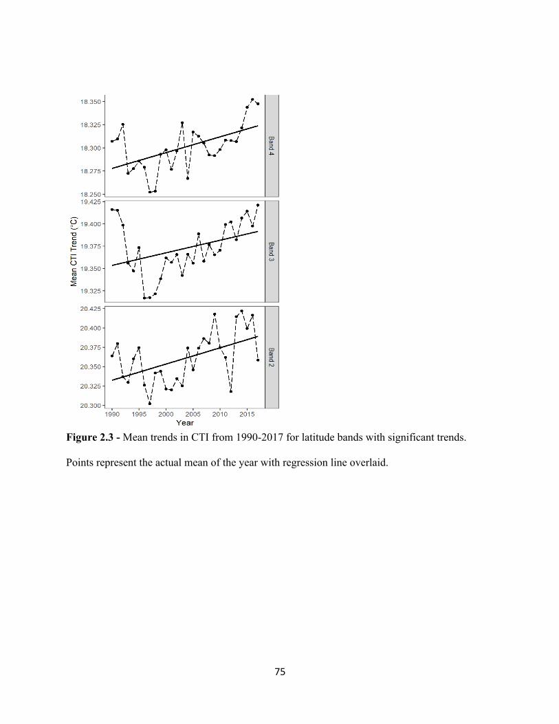
75

Figure 2.3 - Mean trends in CTI from 1990-2017 for latitude bands with significant trends.

Points represent the actual mean of the year with regression line overlaid.

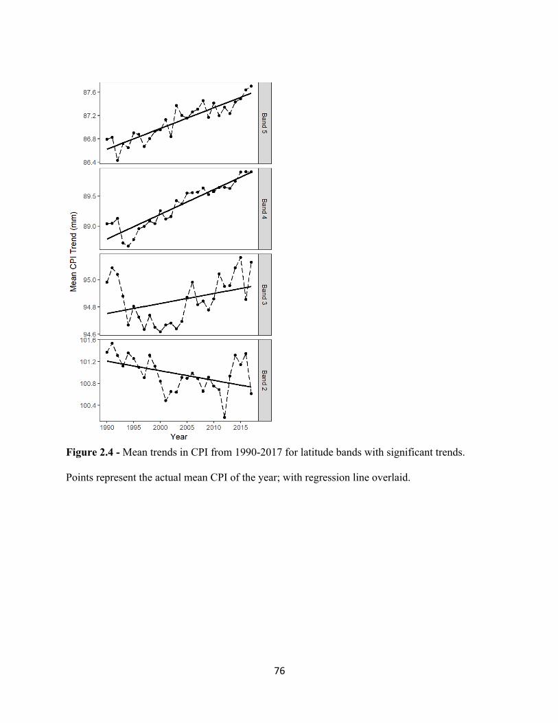
76

Figure 2.4 - Mean trends in CPI from 1990-2017 for latitude bands with significant trends.

Points represent the actual mean CPI of the year; with regression line overlaid.

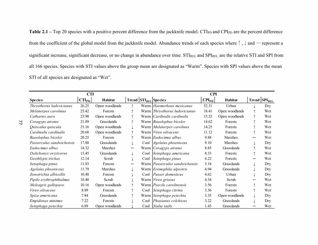
77

Table 2.1 – Top 20 species with a positive percent difference from the jackknife model. CTIPD and CPIPD are the percent difference

from the coefficient of the global model from the jackknife model. Abundance trends of each species where↑,↓and ─ represent a

significant increase, significant decrease, or no change in abundance over time. STIREL and SPIREL are the relative STI and SPI from

all 166 species. Species with STI values above the group mean are designated as “Warm”. Species with SPI values above the mean

STI of all species are designated as “Wet”.

Species CTIPD Habitat Trend STIREL Species CPIPD Habitat Trend SPIREL

Thryothorus ludovicianus 26.25 Open woodlands ↑ Warm Haemorhous mexicanus 52.31 Urban ↓ DryMelanerpes carolinus 25.42 Forests ↑ Warm Thryothorus ludovicianus 18.41 Open woodlands ↑ WetCathartes aura 23.90 Open woodlands ↑ Warm Cardinalis cardinalis 15.32 Open woodlands ↑ WetCoragyps atratus 21.89 Grasslands ↑ Warm Baeolophus bicolor 14.62 Forests ↑ WetQuiscalus quiscula 21.16 Open woodlands ↓ Warm Melanerpes carolinus 14.25 Forests ↑ WetCardinalis cardinalis 20.68 Open woodlands ↑ Warm Vireo olivaceus 11.12 Forests ↑ WetBaeolophus bicolor 20.25 Forests ↑ Warm Eudocimus albus 9.88 Marshes ─ WetPasserculus sandwichensis 17.88 Grasslands ↓ Cool Agelaius phoeniceus 9.10 Marshes ↓ DryEudocimus albus 14.32 Marshes ─ Warm Coragyps atratus 8.85 Grasslands ↑ WetDolichonyx oryzivorus 13.45 Grasslands ↓ Cool Setophaga americana 8.33 Forests ↑ WetGeothlypis trichas 12.14 Scrub ↓ Cool Setophaga pinus 6.22 Forests ─ WetSetophaga pinus 11.83 Forests ─ Warm Passerculus sandwichensis 5.14 Grasslands ↓ DryAgelaius phoeniceus 11.79 Marshes ↓ Warm Eremophila alpestris 4.94 Grasslands ↓ DryZonotrichia albicollis 10.48 Forests ↓ Cool Passer domesticus 4.62 Urban ↓ DryPipilo erythrophthalmus 10.40 Scrub ↓ Warm Vireo griseus 4.34 Scrub ─ WetMeleagris gallopavo 10.16 Open woodlands ↑ Warm Poecile carolinensis 3.56 Forests ↑ WetVireo olivaceus 8.89 Forests ↑ Cool Setophaga citrina 3.36 Forests ↑ WetSpiza americana 7.84 Grasslands ↑ Warm Setophaga petechia 3.35 Open woodlands ↓ DryEmpidonax minimus 7.22 Forests ↓ Cool Phasianus colchicus 3.22 Grasslands ↓ DrySetophaga petechia 6.89 Open woodlands ↓ Cool Sialia sialis 1.45 Grasslands ─ Wet

CTI CPI

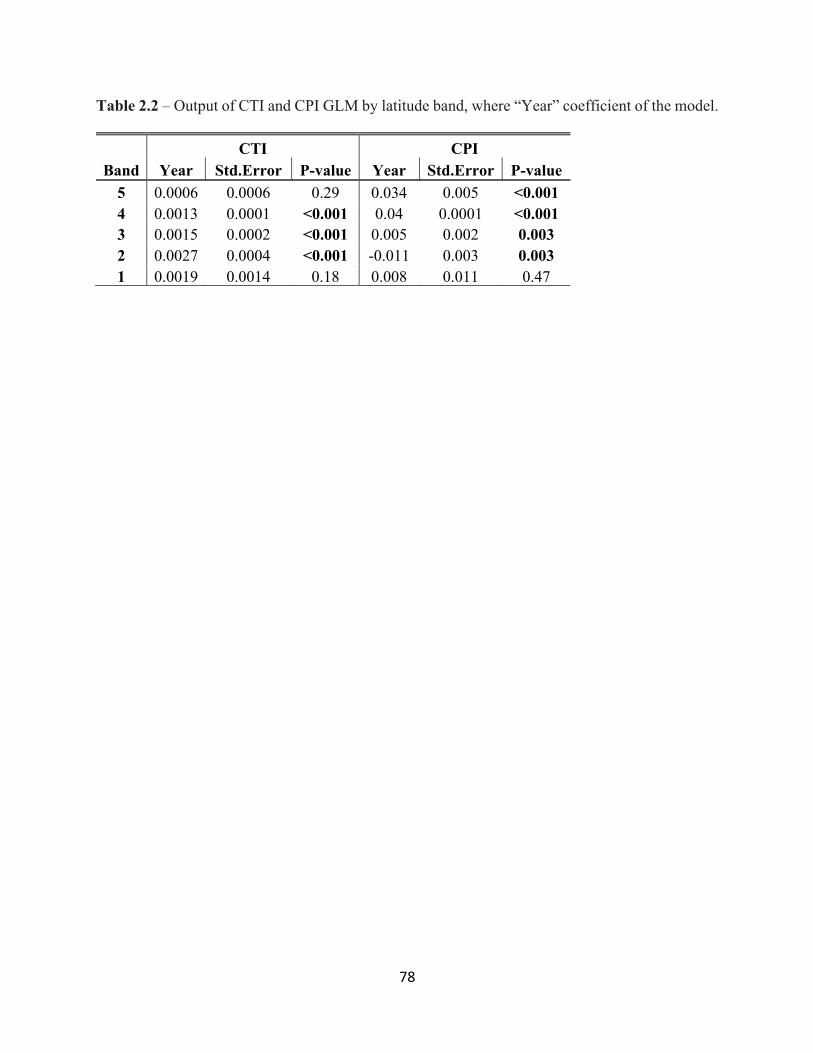
78

Table 2.2 – Output of CTI and CPI GLM by latitude band, where “Year” coefficient of the model.

CTI CPI Band Year Std.Error P-value Year Std.Error P-value

5 0.0006 0.0006 0.29 0.034 0.005 <0.001 4 0.0013 0.0001 <0.001 0.04 0.0001 <0.001 3 0.0015 0.0002 <0.001 0.005 0.002 0.003 2 0.0027 0.0004 <0.001 -0.011 0.003 0.003 1 0.0019 0.0014 0.18 0.008 0.011 0.47

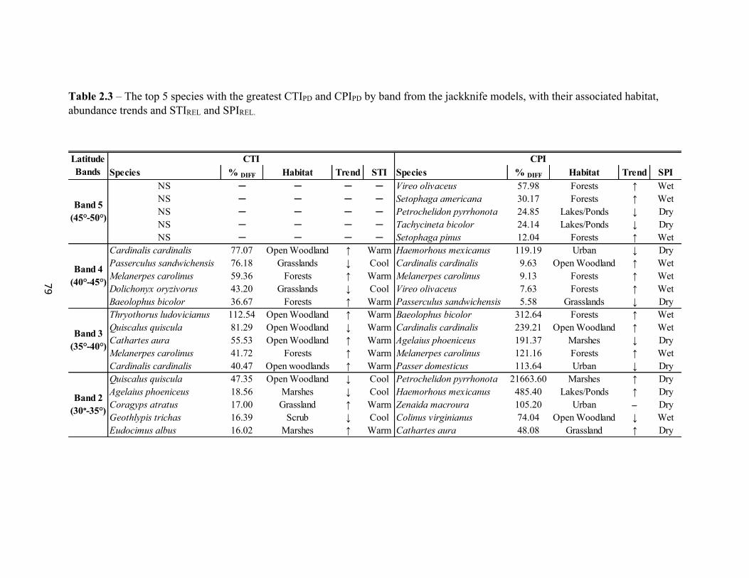
79

Table 2.3 – The top 5 species with the greatest CTIPD and CPIPD by band from the jackknife models, with their associated habitat, abundance trends and STIREL and SPIREL.

Species % DIFF Habitat Trend STI Species % DIFF Habitat Trend SPINS ─ ─ ─ ─ Vireo olivaceus 57.98 Forests ↑ WetNS ─ ─ ─ ─ Setophaga americana 30.17 Forests ↑ WetNS ─ ─ ─ ─ Petrochelidon pyrrhonota 24.85 Lakes/Ponds ↓ DryNS ─ ─ ─ ─ Tachycineta bicolor 24.14 Lakes/Ponds ↓ DryNS ─ ─ ─ ─ Setophaga pinus 12.04 Forests ↑ Wet

Cardinalis cardinalis 77.07 Open Woodland ↑ Warm Haemorhous mexicanus 119.19 Urban ↓ DryPasserculus sandwichensis 76.18 Grasslands ↓ Cool Cardinalis cardinalis 9.63 Open Woodland ↑ WetMelanerpes carolinus 59.36 Forests ↑ Warm Melanerpes carolinus 9.13 Forests ↑ WetDolichonyx oryzivorus 43.20 Grasslands ↓ Cool Vireo olivaceus 7.63 Forests ↑ WetBaeolophus bicolor 36.67 Forests ↑ Warm Passerculus sandwichensis 5.58 Grasslands ↓ DryThryothorus ludovicianus 112.54 Open Woodland ↑ Warm Baeolophus bicolor 312.64 Forests ↑ WetQuiscalus quiscula 81.29 Open Woodland ↓ Warm Cardinalis cardinalis 239.21 Open Woodland ↑ WetCathartes aura 55.53 Open Woodland ↑ Warm Agelaius phoeniceus 191.37 Marshes ↓ DryMelanerpes carolinus 41.72 Forests ↑ Warm Melanerpes carolinus 121.16 Forests ↑ WetCardinalis cardinalis 40.47 Open woodlands ↑ Warm Passer domesticus 113.64 Urban ↓ DryQuiscalus quiscula 47.35 Open Woodland ↓ Cool Petrochelidon pyrrhonota 21663.60 Marshes ↑ DryAgelaius phoeniceus 18.56 Marshes ↓ Cool Haemorhous mexicanus 485.40 Lakes/Ponds ↑ DryCoragyps atratus 17.00 Grassland ↑ Warm Zenaida macroura 105.20 Urban ─ DryGeothlypis trichas 16.39 Scrub ↓ Cool Colinus virginianus 74.04 Open Woodland ↓ WetEudocimus albus 16.02 Marshes ↑ Warm Cathartes aura 48.08 Grassland ↑ Dry

CTI CPI

Band 5 (45°-50°)

Latitude Bands

Band 2 (30°-35°)

Band 3 (35°-40°)

Band 4 (40°-45°)

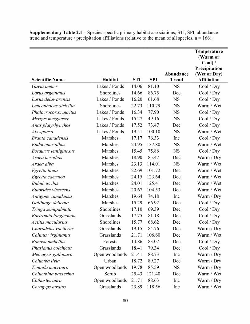
80

Supplementary Table 2.1 – Species specific primary habitat associations, STI, SPI, abundance trend and temperature / precipitation affiliations (relative to the mean of all species, n = 166).

Scientific Name Habitat STI SPI Abundance

Trend

Temperature (Warm or

Cool) / Precipitation (Wet or Dry)

Affiliation Gavia immer Lakes / Ponds 14.06 81.10 NS Cool / Dry Larus argentatus Shorelines 14.66 86.75 Dec Cool / Dry Larus delawarensis Lakes / Ponds 16.20 61.68 NS Cool / Dry Leucophaeus atricilla Shorelines 22.73 110.79 NS Warm / Wet Phalacrocorax auritus Lakes / Ponds 16.34 77.90 NS Cool / Dry Mergus merganser Lakes / Ponds 15.27 49.16 NS Cool / Dry Anas platyrhynchos Lakes / Ponds 17.52 73.47 Dec Cool / Dry Aix sponsa Lakes / Ponds 19.51 100.10 NS Warm / Wet Branta canadensis Marshes 17.17 76.33 Inc Cool / Dry Eudocimus albus Marshes 24.95 137.80 NS Warm / Wet Botaurus lentiginosus Marshes 15.45 75.86 NS Cool / Dry Ardea herodias Marshes 18.90 85.47 Dec Warm / Dry Ardea alba Marshes 23.13 114.01 NS Warm / Wet Egretta thula Marshes 22.69 101.72 Dec Warm / Wet Egretta caerulea Marshes 24.15 123.64 Dec Warm / Wet Bubulcus ibis Marshes 24.01 125.41 Dec Warm / Wet Butorides virescens Marshes 20.67 104.53 Dec Warm / Wet Antigone canadensis Marshes 19.64 74.18 Inc Warm / Dry Gallinago delicata Marshes 15.29 66.92 Dec Cool / Dry Tringa semipalmata Shorelines 17.10 69.39 Dec Cool / Dry Bartramia longicauda Grasslands 17.75 81.18 Dec Cool / Dry Actitis macularius Shorelines 15.77 68.62 Dec Cool / Dry Charadrius vociferus Grasslands 19.15 84.76 Dec Warm / Dry Colinus virginianus Grasslands 21.71 106.60 Dec Warm / Wet Bonasa umbellus Forests 14.86 83.07 Dec Cool / Dry Phasianus colchicus Grasslands 18.41 79.34 Dec Cool / Dry Meleagris gallopavo Open woodlands 21.41 88.73 Inc Warm / Dry Columba livia Urban 18.72 89.27 Dec Warm / Dry Zenaida macroura Open woodlands 19.78 85.59 NS Warm / Dry Columbina passerina Scrub 25.43 121.40 Dec Warm / Wet Cathartes aura Open woodlands 21.71 88.63 Inc Warm / Dry Coragyps atratus Grasslands 23.89 118.56 Inc Warm / Wet

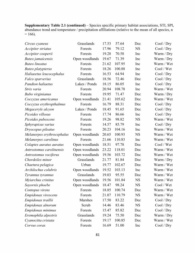
81

Supplementary Table 2.1 (continued) – Species specific primary habitat associations, STI, SPI, abundance trend and temperature / precipitation affiliations (relative to the mean of all species, n = 166). Circus cyaneus Grasslands 17.53 57.64 Dec Cool / Dry Accipiter striatus Forests 17.96 79.12 NS Cool / Dry Accipiter cooperii Forests 19.28 70.58 Inc Warm / Dry Buteo jamaicensis Open woodlands 19.67 71.39 Inc Warm / Dry Buteo lineatus Forests 21.62 107.95 Inc Warm / Wet Buteo platypterus Forests 18.26 100.88 Inc Cool / Wet Haliaeetus leucocephalus Forests 16.53 64.94 Inc Cool / Dry Falco sparverius Grasslands 18.56 72.46 Dec Cool / Dry Pandion haliaetus Lakes / Ponds 18.15 86.05 Inc Cool / Dry Strix varia Forests 20.94 108.78 Inc Warm / Wet Bubo virginianus Forests 19.95 71.47 Dec Warm / Dry Coccyzus americanus Open woodlands 21.41 105.62 Dec Warm / Wet Coccyzus erythropthalmus Forests 16.79 88.31 Dec Cool / Dry Megaceryle alcyon Lakes / Ponds 18.45 91.65 Dec Cool / Dry Picoides villosus Forests 17.74 86.66 Inc Cool / Dry Picoides pubescens Forests 19.26 98.82 NS Warm / Wet Sphyrapicus varius Forests 14.57 85.79 Inc Cool / Dry Dryocopus pileatus Forests 20.23 104.16 Inc Warm / Wet Melanerpes erythrocephalus Open woodlands 20.65 100.93 NS Warm / Wet Melanerpes carolinus Forests 21.66 110.83 Inc Warm / Wet Colaptes auratus auratus Open woodlands 18.51 97.78 Dec Cool / Wet Antrostomus carolinensis Open woodlands 23.22 118.01 Dec Warm / Wet Antrostomus vociferus Open woodlands 19.56 103.72 Dec Warm / Wet Chordeiles minor Grasslands 21.77 81.84 Dec Warm / Dry Chaetura pelagica Urban 19.77 102.67 Dec Warm / Wet Archilochus colubris Open woodlands 19.52 103.13 Inc Warm / Wet Tyrannus tyrannus Grasslands 19.03 95.55 Dec Warm / Wet Myiarchus crinitus Open woodlands 19.56 101.84 NS Warm / Wet Sayornis phoebe Open woodlands 18.47 98.24 NS Cool / Wet Contopus virens Forests 18.85 100.74 Dec Warm / Wet Empidonax virescens Forests 21.07 110.79 NS Warm / Wet Empidonax traillii Marshes 17.50 83.22 Dec Cool / Dry Empidonax alnorum Scrub 14.46 83.46 NS Cool / Dry Empidonax minimus Forests 15.47 85.82 Dec Cool / Dry Eremophila alpestris Grasslands 19.24 75.50 Dec Warm / Dry Cyanocitta cristata Forests 19.17 100.85 Dec Warm / Wet Corvus corax Forests 16.69 51.00 Inc Cool / Dry

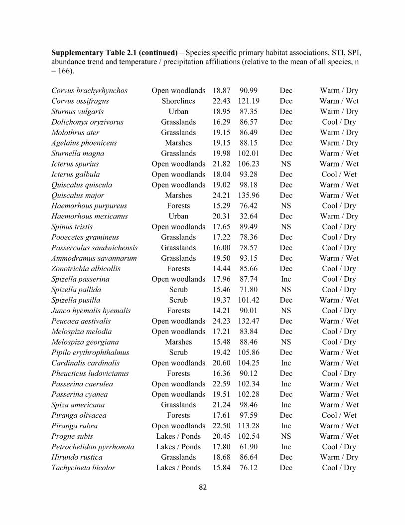
82

Supplementary Table 2.1 (continued) – Species specific primary habitat associations, STI, SPI, abundance trend and temperature / precipitation affiliations (relative to the mean of all species, n = 166). Corvus brachyrhynchos Open woodlands 18.87 90.99 Dec Warm / Dry Corvus ossifragus Shorelines 22.43 121.19 Dec Warm / Wet Sturnus vulgaris Urban 18.95 87.35 Dec Warm / Dry Dolichonyx oryzivorus Grasslands 16.29 86.57 Dec Cool / Dry Molothrus ater Grasslands 19.15 86.49 Dec Warm / Dry Agelaius phoeniceus Marshes 19.15 88.15 Dec Warm / Dry Sturnella magna Grasslands 19.98 102.01 Dec Warm / Wet Icterus spurius Open woodlands 21.82 106.23 NS Warm / Wet Icterus galbula Open woodlands 18.04 93.28 Dec Cool / Wet Quiscalus quiscula Open woodlands 19.02 98.18 Dec Warm / Wet Quiscalus major Marshes 24.21 135.96 Dec Warm / Wet Haemorhous purpureus Forests 15.29 76.42 NS Cool / Dry Haemorhous mexicanus Urban 20.31 32.64 Dec Warm / Dry Spinus tristis Open woodlands 17.65 89.49 NS Cool / Dry Pooecetes gramineus Grasslands 17.22 78.36 Dec Cool / Dry Passerculus sandwichensis Grasslands 16.00 78.57 Dec Cool / Dry Ammodramus savannarum Grasslands 19.50 93.15 Dec Warm / Wet Zonotrichia albicollis Forests 14.44 85.66 Dec Cool / Dry Spizella passerina Open woodlands 17.96 87.74 Inc Cool / Dry Spizella pallida Scrub 15.46 71.80 NS Cool / Dry Spizella pusilla Scrub 19.37 101.42 Dec Warm / Wet Junco hyemalis hyemalis Forests 14.21 90.01 NS Cool / Dry Peucaea aestivalis Open woodlands 24.23 132.47 Dec Warm / Wet Melospiza melodia Open woodlands 17.21 83.84 Dec Cool / Dry Melospiza georgiana Marshes 15.48 88.46 NS Cool / Dry Pipilo erythrophthalmus Scrub 19.42 105.86 Dec Warm / Wet Cardinalis cardinalis Open woodlands 20.60 104.25 Inc Warm / Wet Pheucticus ludovicianus Forests 16.36 90.12 Dec Cool / Dry Passerina caerulea Open woodlands 22.59 102.34 Inc Warm / Wet Passerina cyanea Open woodlands 19.51 102.28 Dec Warm / Wet Spiza americana Grasslands 21.24 98.46 Inc Warm / Wet Piranga olivacea Forests 17.61 97.59 Dec Cool / Wet Piranga rubra Open woodlands 22.50 113.28 Inc Warm / Wet Progne subis Lakes / Ponds 20.45 102.54 NS Warm / Wet Petrochelidon pyrrhonota Lakes / Ponds 17.80 61.90 Inc Cool / Dry Hirundo rustica Grasslands 18.68 86.64 Dec Warm / Dry Tachycineta bicolor Lakes / Ponds 15.84 76.12 Dec Cool / Dry

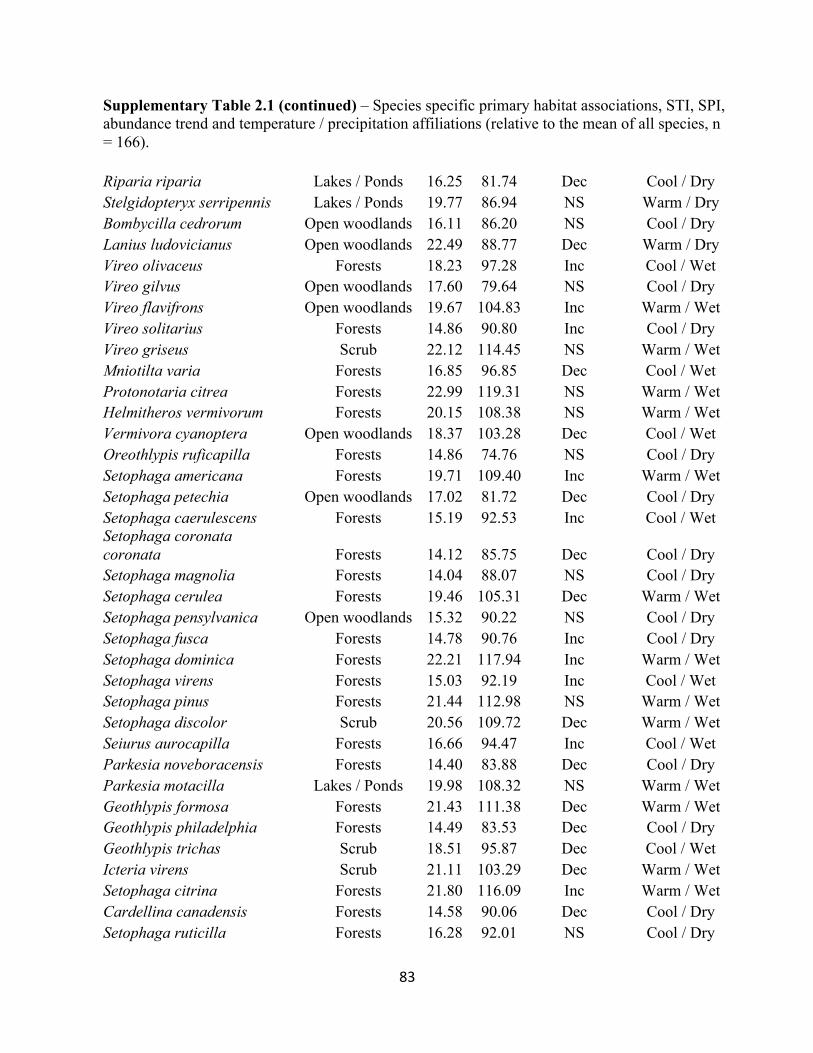
83

Supplementary Table 2.1 (continued) – Species specific primary habitat associations, STI, SPI, abundance trend and temperature / precipitation affiliations (relative to the mean of all species, n = 166). Riparia riparia Lakes / Ponds 16.25 81.74 Dec Cool / Dry Stelgidopteryx serripennis Lakes / Ponds 19.77 86.94 NS Warm / Dry Bombycilla cedrorum Open woodlands 16.11 86.20 NS Cool / Dry Lanius ludovicianus Open woodlands 22.49 88.77 Dec Warm / Dry Vireo olivaceus Forests 18.23 97.28 Inc Cool / Wet Vireo gilvus Open woodlands 17.60 79.64 NS Cool / Dry Vireo flavifrons Open woodlands 19.67 104.83 Inc Warm / Wet Vireo solitarius Forests 14.86 90.80 Inc Cool / Dry Vireo griseus Scrub 22.12 114.45 NS Warm / Wet Mniotilta varia Forests 16.85 96.85 Dec Cool / Wet Protonotaria citrea Forests 22.99 119.31 NS Warm / Wet Helmitheros vermivorum Forests 20.15 108.38 NS Warm / Wet Vermivora cyanoptera Open woodlands 18.37 103.28 Dec Cool / Wet Oreothlypis ruficapilla Forests 14.86 74.76 NS Cool / Dry Setophaga americana Forests 19.71 109.40 Inc Warm / Wet Setophaga petechia Open woodlands 17.02 81.72 Dec Cool / Dry Setophaga caerulescens Forests 15.19 92.53 Inc Cool / Wet Setophaga coronata coronata Forests 14.12 85.75 Dec Cool / Dry Setophaga magnolia Forests 14.04 88.07 NS Cool / Dry Setophaga cerulea Forests 19.46 105.31 Dec Warm / Wet Setophaga pensylvanica Open woodlands 15.32 90.22 NS Cool / Dry Setophaga fusca Forests 14.78 90.76 Inc Cool / Dry Setophaga dominica Forests 22.21 117.94 Inc Warm / Wet Setophaga virens Forests 15.03 92.19 Inc Cool / Wet Setophaga pinus Forests 21.44 112.98 NS Warm / Wet Setophaga discolor Scrub 20.56 109.72 Dec Warm / Wet Seiurus aurocapilla Forests 16.66 94.47 Inc Cool / Wet Parkesia noveboracensis Forests 14.40 83.88 Dec Cool / Dry Parkesia motacilla Lakes / Ponds 19.98 108.32 NS Warm / Wet Geothlypis formosa Forests 21.43 111.38 Dec Warm / Wet Geothlypis philadelphia Forests 14.49 83.53 Dec Cool / Dry Geothlypis trichas Scrub 18.51 95.87 Dec Cool / Wet Icteria virens Scrub 21.11 103.29 Dec Warm / Wet Setophaga citrina Forests 21.80 116.09 Inc Warm / Wet Cardellina canadensis Forests 14.58 90.06 Dec Cool / Dry Setophaga ruticilla Forests 16.28 92.01 NS Cool / Dry

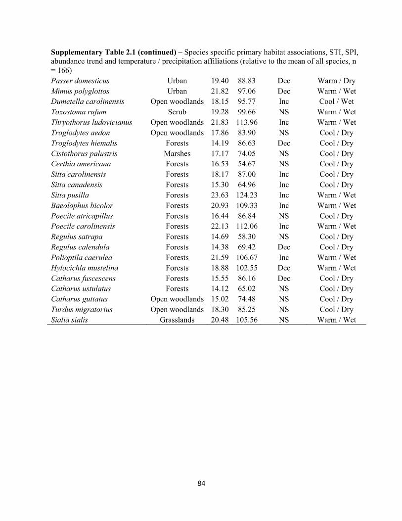
84

Supplementary Table 2.1 (continued) – Species specific primary habitat associations, STI, SPI, abundance trend and temperature / precipitation affiliations (relative to the mean of all species, n = 166) Passer domesticus Urban 19.40 88.83 Dec Warm / Dry Mimus polyglottos Urban 21.82 97.06 Dec Warm / Wet Dumetella carolinensis Open woodlands 18.15 95.77 Inc Cool / Wet Toxostoma rufum Scrub 19.28 99.66 NS Warm / Wet Thryothorus ludovicianus Open woodlands 21.83 113.96 Inc Warm / Wet Troglodytes aedon Open woodlands 17.86 83.90 NS Cool / Dry Troglodytes hiemalis Forests 14.19 86.63 Dec Cool / Dry Cistothorus palustris Marshes 17.17 74.05 NS Cool / Dry Certhia americana Forests 16.53 54.67 NS Cool / Dry Sitta carolinensis Forests 18.17 87.00 Inc Cool / Dry Sitta canadensis Forests 15.30 64.96 Inc Cool / Dry Sitta pusilla Forests 23.63 124.23 Inc Warm / Wet Baeolophus bicolor Forests 20.93 109.33 Inc Warm / Wet Poecile atricapillus Forests 16.44 86.84 NS Cool / Dry Poecile carolinensis Forests 22.13 112.06 Inc Warm / Wet Regulus satrapa Forests 14.69 58.30 NS Cool / Dry Regulus calendula Forests 14.38 69.42 Dec Cool / Dry Polioptila caerulea Forests 21.59 106.67 Inc Warm / Wet Hylocichla mustelina Forests 18.88 102.55 Dec Warm / Wet Catharus fuscescens Forests 15.55 86.16 Dec Cool / Dry Catharus ustulatus Forests 14.12 65.02 NS Cool / Dry Catharus guttatus Open woodlands 15.02 74.48 NS Cool / Dry Turdus migratorius Open woodlands 18.30 85.25 NS Cool / Dry Sialia sialis Grasslands 20.48 105.56 NS Warm / Wet

85

Chapter 3

Functional Community Indices Inform Species Diversity and Changes in Avian Breeding Community Composition in the eastern United States

3.1 ABSTRACT

Climate change has been identified as one of the leading threats to biodiversity and changes

in community composition. Heterogenous responses to climate change can lead to the reshuffling

of community composition over time, resulting in changes in alpha and ß-diversity and the

functional traits of a community, such as the Community Temperature Index (CTI) and the

Community Precipitation Index (CPI), which are measures of how communities are

compositionally composed warm or cool and wet or dry affiliated species. We hypothesize that

the community indices CTI and CPI can be used to inform how changes in species diversity have

changed over time and provide insight as to what ecological drivers are responsible for changes in

species assemblages. Using North American Breeding Bird Survey data collected in the eastern

United States from 1990-2017, we quantified regional and local (along 5 latitude bands) temporal

trends in species richness (α-diversity) and Bray Curtis Dissimilarity (ßBRAY;ß-diversity). We used

a series of Generalized Linear Mixed Models (GLMMs) and Generalized Linear Models (GLMs)

to test if CTI and CPI are predictors to inform α-diversity ß-diversity. To determine if ß-diversity

converged over time we used ANOVA to test if multivariate dispersions of the bands differed from

the group centroid for an early (1990-1994) and a late (2013-2017) time period. At the regional

scale, species richness slightly decreased over the time period and ßBRAY increased. CTI showed

an inverse relationship with species richness, while CPI showed a positive relationship; however,

neither was a good predictor of ß-diversity. Variable patterns in dissimilarity have led to

86

compositional homogenization at the three highest latitude bands. Our results demonstrate that

using community indices in compliment with biodiversity metrics provide greater insight into

community compositional shifts and the underlying ecological drivers of these changes.

3.2 INTRODUCTION

Climate change is one of the biggest threats to biodiversity (Thomas et al. 2004, Bellard et

al. 2012). Poleward shifts in species distributions have occurred at a coarse scale as a response to

changes in climate (Walther et al. 2002, Parmesan & Yohe 2003). However, not all species have

responded equally to climate change (Menendez et al. 2008, Ven der Putten et al. 2010, Chen et

al. 2011), which has resulted in the reshuffling of community assemblages (Devictor et al.

2008, 2012, Bellard et al. 2012, Princé & Zuckerberg 2015). In addition to climate, local-scale

mechanisms such as habitat loss or fragmentation, invasive species and changes to inter or

intraspecific competition regimes can drive changes in patterns of biodiversity (Harley 2011,

Guichard 2017).

Identifying how community assemblages are changing has important implications for

conservation and future planning and management (Gaüzère et al. 2016, Socolar et al. 2016,

Fourcade et al. 2019). Northward range expansion is recognized as an ecological indicator of

climate change (Thomas & Lennon 1999, Parmesan & Yohe 2003, La Sorte & Thompson 2007,

Brommer 2008, Reif et al. 2010). These northward expansions are predicted to impact diversity

in several ways. First, generalist and abundant species should expand their ranges more readily

and rapidly than specialized species (McKinney & Lockwood 1999, Davey et al. 2012), leading to

an initial increase in species richness at the local community level (Filippi-Codaccioni et

al. 2010). Second, communities should become increasingly composed of northward-moving

species originating from warmer climatic regions, when compared to the original community

87

structure (Devictor et al. 2008). Third, communities should become more taxonomically similar

(homogenized) over time and space as competitive species successfully colonize and replace

previously established species (McKinney & Lockwood 1999, La Sorte & McKinney 2007).

With respect to climate, community indices are used to investigate the temporal changes

in the functional traits of a community. The Community Temperature Index (CTI) measures the

weighted contribution of warmer vs cooler dwelling species within a community (Devictor et

al. 2008, Devictor et al. 2012), and is widely used for this purpose. CTI is calculated as a

weighted average of each species’ Species Temperature Index (STI). STI is the average

temperature over a species entire range, thus reflecting its thermal envelope (Thuiller et al. 2005,

Hijmans & Graham 2006, Jiguet et al. 2007). Similarly, a Community Precipitation Index (CPI)

taking the average precipitation (mm) over a species range, measures if wet versus dry dwelling

species are changing abundances in a community (see Chapter 2). Positive trends in CTI have been

attributed to increased abundances of warm-dwelling species moving into a community

(Devictor et al. 2008, 2012, Lindström et al. 2013, Princé & Zuckerberg 2015), or decreased

abundance as cool-dwelling species decrease (Oliver et al. 2017). Similarly, CPI has also been

shown to increase with an increased abundance of warm-dwelling species at higher latitude bands

(Curley et al. in press)

Species richness is a measure of biodiversity that is used to assess diversity at the site or

local level (α-diversity; Gotelli & Colwell 2001). Species richness is a count of the number of

species in a community, that does not incorporate abundances. Though widely used in the field of

ecology due to its ease of measurement and interpretation, meta-analyses show that community

composition changes over time without a net change in species richness (Vellend et al. 2013,

Dornelas et al. 2014, Hillebrand et al. 2018). Therefore, species richness may be an overly

88

simplified indicator for informing temporal trends in biodiversity because of its limited ability to

detect underlying ecological processes (Whittaker et al. 2001, Washington 2003, Devictor &

Robert 2008). However, species richness in compliment with other measures of biodiversity, such

as community indices that incorporate abundance, can elucidate the ecological mechanism driving

community change (Aviron et al. 2007, Filippi-Codaccioni et al. 2010).

ß-diversity is often used to link the spatial and/or temporal structure of species assemblages

to underlying ecological processes, such as species turnover (Basegla 2010, Legendre 2013). A

pattern that may emerge from changes in ß-diversity is biotic homogenization, a process where

species assemblages become increasingly similar over time or space (Olden & Rooney 2006).

Biotic homogenization has been a documented response to anthropogenic disturbance,

urbanization, and habitat fragmentation (McKinney 2006). Biotic homogenization has been

characterized as an increase of generalist (common) species and/or extinction of more specialized

species (McKinney & Lockwood 1999). Under current warming trends, generalist species may

respond more rapidly to increased current warming trends (Davey et al. 2012), and thus more

greatly contribute to changes in community assemblage (Reif et al. 2010).

In Chapter 2, I asked how climate can influence diversity by separating “climate” into its

temperature and rainfall components using CTI and CPI, respectively. In this study we examined

the interplay among these community indices and measures of alpha and ß-diversity in

communities of eastern North American birds and ask how these measures might predict continued

community response to climate change. In this study we test several hypotheses; first, we

hypothesize that communities with high CTI and CPI values are less diverse. From previous

literature, we expect negative relationship between diversity and CTI and CPI, as generalist species

saturate community composition via southern-dwelling species moving north. Second, we test the

89

hypothesis that communities have not temporally changed in their species composition. If temporal

changes have community composition, we can expect that species turnover and/or species loss are

occurring. Lastly, we test that communities have become more homogenized over time. We

propose a mechanism driving community changes of North American birds; that the observed

increase in CTI and CPI as documented in Chapter 2 from the northward expansion of southern

species, has led to increased species turnover at mid latitudes, making community structure

between communities to beginning to resemble each other from a south to north direction.

3.3 METHODS

3.3.1 Community Data - Breeding Bird Survey and Study Design

Avian community data was obtained from The North American Breeding Bird Survey

(BBS; US Geological Survey Patuxent Wildlife Research Center, 2017) for the eastern United

States between -90° to -60° longitude (east of the Mississippi River) and between 25° to 50°

latitudes, from the years 1990 to 2017. The BBS is conducted in June during the avian breeding

season. Each BBS route is 39.4 km long with 50 three-minute point count locations spaced

throughout. We applied a temporal filter to exclude routes missing two or more consecutive years

of sampling. The temporal filter reduced the spatial and temporal bias inherent of a multisite,

largescale dataset. Each BBS route was treated as a single community, where the abundances of

each species was totaled for all 50-point counts. Diversity and community calculations were done

at a regional scale, which we define as all BBS routes in the eastern United States, as well as at the

local scale, where the study site was partitioned into 5° latitude bands (Figure 3.1).

3.3.2 Species Selection and Classification

For the initial species pool, we followed the current taxonomy of North American birds

implemented by the American Ornithologists' Union (AOU 2018). To ensure that only well-

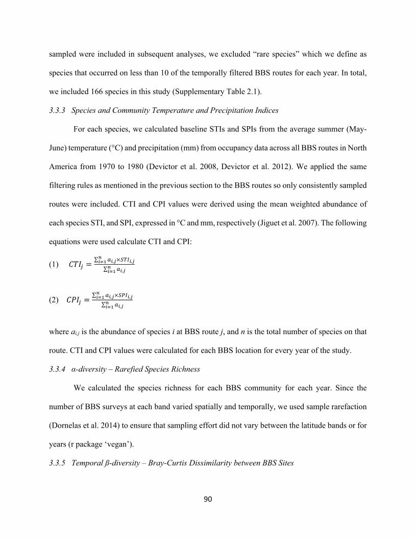
90

sampled were included in subsequent analyses, we excluded “rare species” which we define as

species that occurred on less than 10 of the temporally filtered BBS routes for each year. In total,

we included 166 species in this study (Supplementary Table 2.1).

3.3.3 Species and Community Temperature and Precipitation Indices

For each species, we calculated baseline STIs and SPIs from the average summer (May-

June) temperature (°C) and precipitation (mm) from occupancy data across all BBS routes in North

America from 1970 to 1980 (Devictor et al. 2008, Devictor et al. 2012). We applied the same

filtering rules as mentioned in the previous section to the BBS routes so only consistently sampled

routes were included. CTI and CPI values were derived using the mean weighted abundance of

each species STI, and SPI, expressed in °C and mm, respectively (Jiguet et al. 2007). The following

equations were used calculate CTI and CPI:

(1) !"#$ =∑ '(,*×,-.(,*/(01∑ '(,*/(01

(2) !3#$ =∑ '(,*×,4.(,*/(01∑ '(,*/(01

where ai,j is the abundance of species i at BBS route j, and n is the total number of species on that

route. CTI and CPI values were calculated for each BBS location for every year of the study.

3.3.4 α-diversity – Rarefied Species Richness

We calculated the species richness for each BBS community for each year. Since the

number of BBS surveys at each band varied spatially and temporally, we used sample rarefaction

(Dornelas et al. 2014) to ensure that sampling effort did not vary between the latitude bands or for

years (r package ‘vegan’).

3.3.5 Temporal ß-diversity – Bray-Curtis Dissimilarity between BBS Sites

91

Bray-Curtis Dissimilarity (ßBRAY) is an abundance-based dissimilarity index used to

quantify species variation between sites. ßBRAY values range from 0 to 1; where 0 indicates that

community composition between 2 communities is identical and a value of 1 if they do not share

any species in common. ßBRAY can be partitioned into two components: Balanced variation

(βBC.BAL; species turnover) and abundance gradient (βBC.GRA; nestedness), the sum of which is equal

to the total dissimilarity (see Baselga 2010, 2013). Balanced variation is related to species

replacement and reflects species gain and loss from ecological drivers such as environmental

filtering, competition and historical events (Leprieur et al. 2011). The abundance gradient

component is a richness pattern where species-poor locations are subsets of richer community

assemblages, highlighting species losses between locations (Basegla 2013). We used R package

‘betapart’ (Baselga et al. 2017) to calculate ßBRAY distance matrices between all BBS locations for

each year of the study at the regional scale and again at the local scale). We partitioned βBRAY into

its to components of balanced variation (βBC.BAL) and abundance gradient (βBC.GRA)

(Baselga 2013, 2017). βBRAY, βBC.BAL and βBC.GRA values were averaged across their respective

distance matrices to obtain a single value per year regionally, and at each latitude band. We

regressed ßBRAY, βBC.BAL, and βBC.GRA separately against time to detect: 1) temporal patterns in ß-

diversity and 2) it this temporal pattern consistent with temporal changes in the balanced variation

between location and abundance gradient.

3.3.6 CTI and CPI as predictors of alpha and ß-diversity

To test for a regional spatiotemporal relationship of CTI and CPI on α-diversity we used

Generalized Liner Models (GLMMs) where ‘Year’ and ‘Latitude’ were included as fixed

covariates and BBS sites as a random term (Zuur 2009; r package ‘nlme’). We then reran this

model at the local scale but removed the ‘Latitude’ variable because this was accounted for in the

92

structuring of the latitude bands. To test of the spatiotemporal relationship of our community

indices to ß diversity we used GLMs to test the relationship of ßBRAY, βBC.BAL, and βBC.GRA to mean

CTI and CPI as predictors and using year as a continuous variable.

3.3.7 Temporal Trends in Community Dissimilarity – Bray Curtis Dissimilarity comparison

between bands

To investigate if latitudes bands were becoming more homogenized over time, we tested

the multivariate dispersions (variances) for each of the latitude bands from the total group centroid

and conducted an ANOVA test if the distances of one or more of the groups were different to the

group centroid. To do this, we partitioned our community dataset between an earlier time period

from 1990-1994 and a later period from 2013-2017. Between-band comparisons for each time

period we used Tukey’s Honest Significant Differences between groups (r package ‘vegan’).

3.4 RESULTS

3.4.1 Rarefied Species Richness at the Regional Scale

At the regional scale, ‘Year’, ‘CTI’, ‘CPI’ and ‘Latitude’ were all significant predictors of

rarified species richness for avian communities in the eastern United States (Table 3.1). We

observed an overall decline in species richness over the time period. CTI was negatively related to

richness (p = <0.001) and CPI was positively related (p = <0.001). There was positive relationship

of species richness to latitude (P = 0.001) (Table 3.1).

3.4.2 Rarefied Species Richness at the Local Scale

CTI and CPI were not significant predictors at every latitude band but when they were,

each showed a consistent relationship (Table 3.2). CTI has a significantly negative relationship

with species richness at bands 2 – 4. CPI had a significantly positive relationship with species

93

richness from bands 2 – 5 (Table 3.2). We found no significant relationship of mean CTI and CPI

as predictors of mean ßBRAY, βBC.BAL, and βBC.GRA at the regional or local scales.

3.4.3 Bray Curtis Dissimilarity

From our GLMs, we found no significant relationship of mean CTI and CPI as predictors

of mean ßBRAY, βBC.BAL, and βBC.GRA at the regional or local scales, however, there were significant

temporal trends in ß-diversity. At the regional scale, Bray Curtis Dissimilarity has significantly

increased during the time period (0.0002 ± 0.00007, t‐value = 2.91, P = 0.007, Figure 3.1a), albeit,

at a very slow annual rate. There was no temporal trend of βBC.BAL (Figure 3.1b) but a positive

significant trend in βBC.GRA (0.00018 ± 0.00007, t‐value = 3.193, P = 0.00367, Figure 3.1c)

indicating that increased dissimilarity between communities is due to an increase of species loss

or local extinction over time.

At the local scale, ßBRAY increased at bands 1, 2 and 4, and decreased at band 5 (Figure 3.2,

left panel). βBC.BAL was always the larger component of ßBRAY, and has significant temporal trends

at each latitude band. Bands 1, 3 and 4 had positive trends in βBC.BAL and bands 2 and 5 had

significantly negative temporal trends (Figure 3.2, middle panel). βBC.GRA was almost the smaller

component of ßBRAY at each latitude band. We found a significant positive relationship at band 2

and a negative relationship at band 3 (Figure 3.2, right panel).

3.4.4 Temporal Trends in Community Dissimilarity – Bray Curtis Dissimilarity comparison

between bands

In the first time period, the distance from group to centroid for bands 3 and 4 was not

significantly different (P = 0.76) and the distance from bands 4 and 5 was only marginally similar

(P = 0.06). In the later time period, the distance from group to centroid was smaller for bands 3 -

94

5. The lowest latitude bands remained dissimilar over time period, whereas, the mid and northern-

most bands become more similar in composition over time (Figure 3.3).

3.5 DISCUSSION

Avian community composition in the eastern United States changed over the study period.

Regional changes in community assemblages appear to be driven by non-uniform trends of α and

ß-diversity at the local scale. The variability in the observed patterns of α and ß-diversity at

different scales suggests that multiple differences in ecological drivers are shaping community

assemblages and that these processes are not uniform across the study region (La Sorte 2006,

Mimet et al. 2019). While a variety of small-scale drivers may be shaping community composition,

biotic homogenization across higher latitudes was observed. The complimentary analyses (Using

CTI / CPI) in this study provide support that homogenization has occurred as a result of northward

range expansion of generalist and common species. CTI and CPI served as useful predictors of α-

diversity at both the regional and local scales, and are useful in implying how ß-diversity is

changing.

3.5.1 Temporal Changes in Species Richness at the Regional and Local Scales

At the regional scale, there was a gradual decline of species richness, but larger, non-

uniform trends observed within the local bands. Patterns of species richness are often dependent

on the scale of the study (Sax & Gaines 2003, Vellend et al. 2013, Dornelas et al. 2014). Previous

studies reported similar patterns of species richness which are attributed to positive and negative

slopes at the local scale leading to no net loss of average richness at the regional scale (Vellend et

al. 2013, Dornelas et al. 2014, Elahi et al. 2015, Yoccoz et al. 2018). However, different patterns

of local richness have important implications for regional scale biodiversity. For example, species

richness decreased at the highest latitude band, and area where richness was previously high. This

95

convergence of species richness between latitude bands lends support to the biotic homogenization

we observed between bands 5 and 3 (Van Turnhout et al. 2007). Initial increases in species richness

have been attributed to the range expansion and/or colonization of generalist species (Blackburn

et al. 2004, Christian et al. 2009), which explains why band 3 is the only band showing a significant

increase in richness. The variation we observed on the local scale without an observed change in

richness at the regional scale suggests that using simple measures of species richness masks

distinctive ecological processes operating at the local scale. Concurrent use of community indices

provided greater insight as to how community composition has changed.

3.5.2 The Relationship Between Community Indices and Species Richness

In this study, we found a negative relationship between species richness and CTI. In

general, as community richness decreases, there is a simultaneous increase in CTI. This pattern is

consistent with the northward expansion of southernly distributed, warm-dwelling species

(Menéndez et al. 2006, Devictor et al. 2008, Princé & Zuckerberg 2015, Curley et al. in press) and

the gradual replacement of species with low STI values by species with higher STI values (Jiguet

et al. 2010, Lindström et al. 2013). Recent studies corroborate this pattern of increasing CTI

related to species turnover (Lindström et al. 2013, Fourcade et al. 2019) and increased abundance

trends of warm-dwelling, common species (see Chapter 2). Conversely, we found a positive

relationship between CPI and richness, indicating a decoupling of these two indices. Previous

studies found positive associations with precipitation and species richness (Van Rensburg et al.

2002). Species richness has declines at the regional scale and at all latitude bands richness has

generally declined at the regional scale and at all latitude bands except for band 3. Our results

indicate two different processes might be occurring that are not mutually exclusive. First, a smaller

number of species are responding to changes in precipitation in comparison to temperature

96

(Pearce-Higgins et al. 2015). Second, some habitat types might be more sensitive to changes in

precipitation than others, but do not occur widespread enough to sway the overall declines in

richness that we observed.

3.5.3 Temporal Changes in ß-diversity at the Regional and Local Scales

Mean ßBRAY increased at the regional scale. The βBC.BAL component was proportionally

higher but exhibited no linear trend, whereas the βBC.GRA component significantly increased. It

appears that the driving force in the increased dissimilarity between communities at the regional

scale is driven by the βBC.GRA component. Temporal changes in βBC.BAL appear to occur as species

ranges expand, whereas βBC.GRA might reflect contributions of colonization and extinction events

in community assemblages (Whittaker & Fernandez‐Palacios 2007, Leprieur et al. 2009). The

temporal trend in the βBC.GRA suggests that species loss is increasingly important in community

dynamics, while species turnover remains constant.

Variable patterns emerged when we scaled down to the different latitude bands. Bands 1,

2 and 4 had positive trends in ßBRAY. Band 5 was the only band with a negative trend in ßBRAY.

This variation in ß-diversity was in part explained by differences in the βBC.BAL and βBC.GRA

components. βBC.BAL was consistently the highest component of ßBRAY and had significant

temporal trends at each latitude band, indicating that community composition continuously

changed from the original time period (Dornelas et al. 2014). Our observed patterns suggest that a

loss of species at some latitudes and northward expansion of species are occurring simultaneously,

reflected by our positive trends in turnover at mid latitudes, and a negative trend at the highest

latitude band. Temporal relationships of the βBC.BAL and βBC.GRA components have important

implications for the factors diving biotic homogenization, particularly if turnover trends are non-

uniform between locations (Rooney et al. 2007)

97

3.5.4 Biotic Homogenization

ß-diversity between communities is expected to be more dissimilar with greater geographic

separation (Nekola & White, 1999). During the earlier time period, adjacent Bands 3 and 4 were

the only bands that were not significantly different from the group centroid. However, during the

later time period, bands 3 through 5 (~1, 660 km distance) converged on the group centroid.

Similar patterns in homogenization between latitude bands have been observed with marine fish

(Magurran et al. 2015). Biotic homogenization is attributed to decreases in habitat specialists or

increases in habitat generalists, each of which can occur simultaneously (Olden & Poff, 2003,

Rooney et al. 2004). Well documented range shifts in North American birds are potentially

contributing to the turnover observed at this scale (Thomas & Lennon 1999, La Sorte & Thompson

2007, Curley et al. in press). This should lead to an initial increase in richness at the local scale

(La Sorte 2006), but result in long-term homogenization with expansion of generalist species (La

Sorte & Boecklen, 2005, La Sorte 2006).

North America avifauna is experiencing steep and staggering declines (Rosenberg et al.

2019), which have impacted biodiversity and community composition. By employing the use of

multiple community indices concurrently, this study provides a mechanism in which avian

communities have become homogenized. In Chapter 2, we found that increases in CTI and CPI

were driven by northward-moving species originating from warmer climatic regions. At the mid

latitudes of this study (bands 3&4), species turnover had significantly increased, driven primarily

by northward increases in southerly distributed, locally-common species, such as Northern

Cardinal (Cardinalis cardinalis), Carolina Wren (Thryothorus ludovicianus), Red-bellied

woodpecker (Melanerpes carolinus) and Tufted Titmouse (Baeolophus bicolor) (Chapter 2) and

decreases in northern species, such as Savannah Sparrow (Passerculus sandwichensis) and

98

Bobolink (Dolichonyx oryzivorus). As southern species continue to move north as indicated by

the positive temporal trends of turnover at mid latitudes, and northward latitudes decreasing in

community composition, we expect biotic homogenization to continue across these latitude

bands.

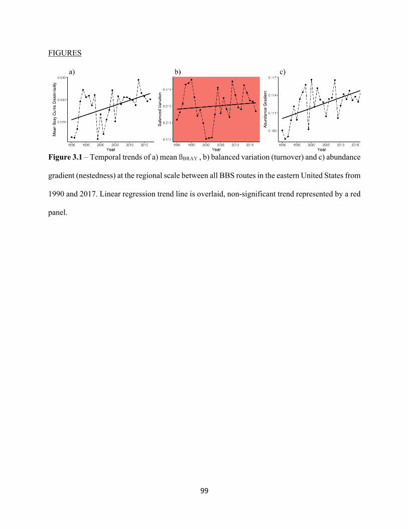
99

FIGURES

Figure 3.1 – Temporal trends of a) mean ßBRAY , b) balanced variation (turnover) and c) abundance

gradient (nestedness) at the regional scale between all BBS routes in the eastern United States from

1990 and 2017. Linear regression trend line is overlaid, non-significant trend represented by a red

panel.

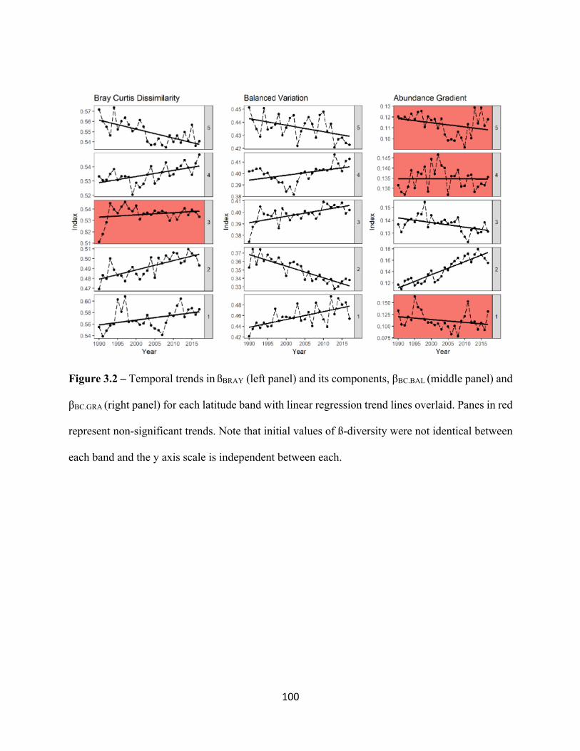
100

Figure 3.2 – Temporal trends in ßBRAY (left panel) and its components, βBC.BAL (middle panel) and

βBC.GRA (right panel) for each latitude band with linear regression trend lines overlaid. Panes in red

represent non-significant trends. Note that initial values of ß-diversity were not identical between

each band and the y axis scale is independent between each.

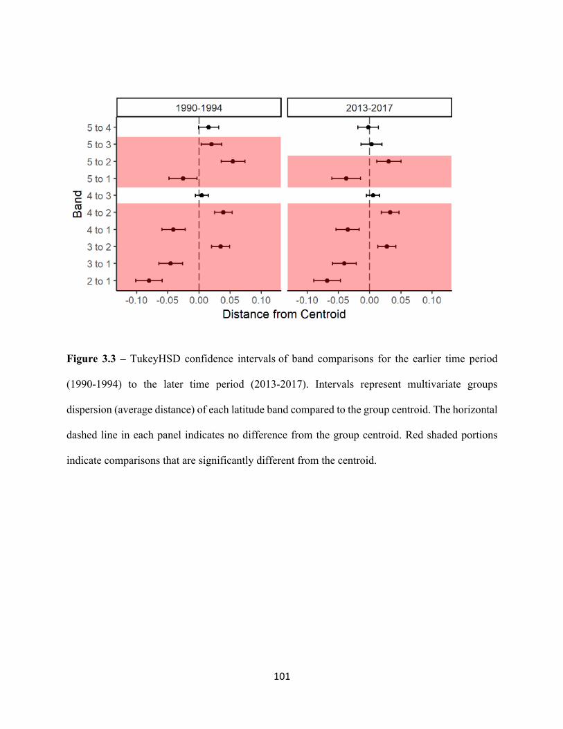
101

Figure 3.3 – TukeyHSD confidence intervals of band comparisons for the earlier time period

(1990-1994) to the later time period (2013-2017). Intervals represent multivariate groups

dispersion (average distance) of each latitude band compared to the group centroid. The horizontal

dashed line in each panel indicates no difference from the group centroid. Red shaded portions

indicate comparisons that are significantly different from the centroid.

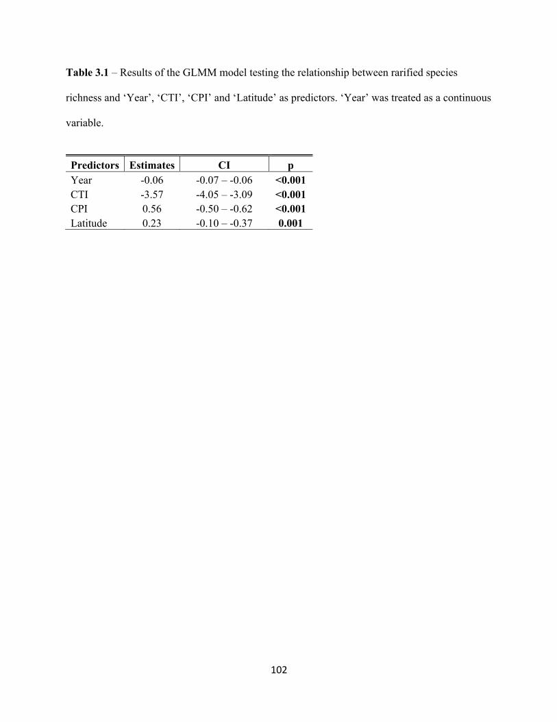
102

Table 3.1 – Results of the GLMM model testing the relationship between rarified species

richness and ‘Year’, ‘CTI’, ‘CPI’ and ‘Latitude’ as predictors. ‘Year’ was treated as a continuous

variable.

Predictors Estimates CI p Year -0.06 -0.07 – -0.06 <0.001 CTI -3.57 -4.05 – -3.09 <0.001 CPI 0.56 -0.50 – -0.62 <0.001 Latitude 0.23 -0.10 – -0.37 0.001

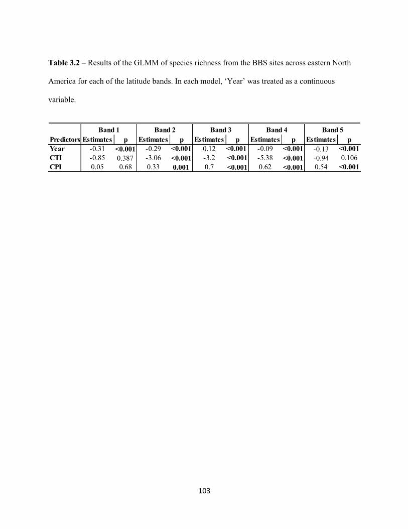
103

Table 3.2 – Results of the GLMM of species richness from the BBS sites across eastern North

America for each of the latitude bands. In each model, ‘Year’ was treated as a continuous

variable.

Estimates p Estimates p Estimates p Estimates p Estimates pYear -0.31 <0.001 -0.29 <0.001 0.12 <0.001 -0.09 <0.001 -0.13 <0.001CTI -0.85 0.387 -3.06 <0.001 -3.2 <0.001 -5.38 <0.001 -0.94 0.106CPI 0.05 0.68 0.33 0.001 0.7 <0.001 0.62 <0.001 0.54 <0.001

Band 5Predictors

Band 1 Band 2 Band 3 Band 4

104

Conclusion This body of this dissertation focuses on changes in species distributions under

anthropogenic climate change and how these changes have impacted community dynamics and

diversity patterns for North American birds. The following text summarizes the intellectual merit

of each chapter and contributions to the field. I offer future directions on where this research can

be expanded.

Chapter 1 focuses on inter-seasonal distribution shifts for short-distance migratory birds

and the impacts these shifts have on migratory distances. This represents the first study of North

American birds that evaluates differences in winter and breeding range shifts from a

macroecological perspective and provides evidence that migration distances are potentially

changing for many species. At the spatial resolution of the climate data, winter “stationary” COAs

have, overall, decreased in temperature and precipitation but have not changed at the annual

shifting COAs. During the breeding season, temperature has increased at the “stationary” and

“shifting annual” COAs but precipitation has not changed in each. The changes in temperature and

precipitation are only in regards to COAs of each species and do not incorporate what each species

is experiencing over their entire range. I suggest that the incorporation of climate conditions over

entire species’ range in comparison to the centroid will provide greater insight to changing

condition and inclusions of more climate variables (such as temperature extremes) and time lags,

which have shown to influence avian distributions. Lastly, this chapter also has applications for

individual species studies, and offers preliminary expectations that can be used to ground-truth

migration studies.

Chapter 2 evaluates how the compositions of communities during the avian breeding

season are changing by evaluating trends in functional community indices, the Community

105

Temperature Index (CTI; Devictor et al. 2008) and the newly developed Community Precipitation

Index (CPI). This study intended to compliment and compare to the positive CTI trends that have

been observed in a previous study of winter avian communities of eastern North America (Princé

& Zuckerberg 2015), as well as to establish a community index that reflects changes in

precipitation-affiliations of birds. We expanded on this previous study by including a larger pool

of species, and species-specific traits and abundance trends, as predictors of species-specific

contributions to community change. Our study reports similar trends in CTI via a similar

mechanism; warm-dwelling, southern species have expanded into communities at higher latitudes.

By incorporating species-specific traits and abundance trends, we also attribute changes in CTI

and CPI to declines in cool-dwelling species, grassland species and species that are associated with

urban habitats. A greater number of species have impacted CTI, while fewer species have impacted

the CPI, which suggests that species dwelling in different habitat types (e.g. grasslands, where

precipitation is more limited) are responding differently to climate change. This result offers the

potential for follow-up research at a finer scale that incorporates land use changes and different

habitat types with these two community indices (Kampichler et al. 2012).

In Chapter 3, I tested the applications of these community indices as predictors of

biodiversity at both a regional and local scales. I found that increasing CTI is associated with

decreases in species richness, which reflects turnover of species with a low STI values with species

with a higher STI values (see Chapter 2). This replacement of cool-dwelling species with warm-

dwelling species is consistent with climate change (Davey et al. 2012). An interesting result was

that the relationship between species richness and CPI was significantly positive. This reveals a

decoupling of CTI and CPI indices, suggesting that in at least some environments, species are

responding more strongly to precipitation, though the overall trend of species richness was

106

negative. This divergent relationship to species richness between the two indices highlights that

species-specific traits, or specialized species, must be contributing to community composition but

on a smaller scale. The relationships of specialized species response to changes in precipitation

would be an interesting next step, particularly in regards to habitat types. Lastly, the

complimentary results of α and ß diversity from this chapter lend strong support to the idea that

communities at higher latitudes are becoming increasingly homogenized. Identifying specific

areas (via decomposing the distance matrices by pairs) would be an informative and useful follow

up study, which I intend to begin in 2020.

The goals of this dissertation were to help inform gaps in the lack of inter-seasonal studies

and assessment of individual species contributions to community changes. Inter-seasonal studies

are challenging in large part due to the lack of comparable datasets at large spatial scales (Runge

et al. 2014). However, spatiotemporal variability between seasons should be used to inform

conservation strategies. Individual species contributions to these large-scale patterns are important

in informing and identifying how populations and communities are changing under this climate

regime.

107

Bibliography Ahola, M., Laaksonen, T., Sippola, K., Eeva, T., Rainio, K., & Lehikoinen, E. (2004). Variation in climate warming along the migration route uncouples arrival and breeding dates. Global Change Biology, 10(9), 1610-1617. Alerstam, T., Hedenström, A., & Åkesson, S. (2003). Long‐distance migration: evolution

and determinants. Oikos, 103(2), 247-260. Alerstam, T., & Lindström, Å. (1990). Optimal bird migration: the relative importance of time,

energy, and safety. In Bird migration (pp. 331-351): Springer. Alexander, J. M., Diez, J. M., & Levine, J. M. (2015). Novel competitors shape species’ responses to climate change. Nature, 525(7570), 515. Ash, J. D., Givnish, T. J., & Waller, D. M. (2017). Tracking lags in historical plant species’ shifts

in relation to regional climate change. Global change biology, 23(3), 1305-1315. Aviron, S., Jeanneret, P., Schüpbach, B., & Herzog, F. (2007). Effects of agri-environmental

measures, site and landscape conditions on butterfly diversity of Swiss grassland. Agriculture, ecosystems & environment, 122(3), 295-304.

Baselga, A. (2010). Partitioning the turnover and nestedness components of beta diversity. Global ecology and biogeography, 19(1), 134-143. Baselga, A. (2013). Separating the two components of abundance‐based dissimilarity: balanced changes in abundance vs. abundance gradients. Methods in Ecology and Evolution, 4(6), 552-557. Baselga, A., Orme, D., Villeger, S., De Bortoli, J., & Leprieur, F. (2017). Partitioning beta diversity into turnover and nestedness components. Package betapart, Version, 1-4. Bauer, S., & Hoye, B. J. (2014). Migratory animals couple biodiversity and ecosystem functioning

worldwide. Science, 344(6179), 1242552. Bellard, C., Bertelsmeier, C., Leadley, P., Thuiller, W., & Courchamp, F. (2012). Impacts of climate change on the future of biodiversity. Ecology letters, 15(4), 365-377. Berger, J. J. C. B. (2004). The last mile: how to sustain long‐distance migration in mammals. 18(2),

320-331. Bock, C. E. and L. W. Lepthien. (1976). Growth in the eastern House Finch population, 1962-

1971. American Birds 30:791-792. Both, C., & Visser, M. E. (2001). Adjustment to climate change is constrained by arrival date in a

long-distance migrant bird. Nature, 411(6835), 296–298. Both, C., Van Turnhout, C. A., Bijlsma, R. G., Siepel, H., Van Strien, A. J., & Foppen, R. P.

(2009). Avian population consequences of climate change are most severe for long-distance migrants in seasonal habitats. Proceedings of the Royal Society B: Biological Sciences, 277(1685), 1259-1266.

Brennan, L. A. (1991). How can we reverse the northern bobwhite population decline? Wildlife Society Bulletin 19: 544– 555. Brommer, J. E. (2008). Extent of recent polewards range margin shifts in Finnish birds depends on their body mass and feeding ecology. Ornis Fennica, 85(4), 109-17. Brown, C. R., M. B. Brown, P. Pyle, and M.A. Patten. (2017) Cliff Swallow (Petrochelidon pryyhonota), version 3.0. In The Birds of North America (P. G. Rodewald, Editor). Cornell Lan of Ornithology, Ithaca, NY, USA. https://dio.ord/10.2173/bna.cliswa.03 Burger, J., & Gochfeld, M. (2004). Marine birds as sentinels of environmental

pollution. EcoHealth, 1(3), 263-274.

108

Carroll, I. T., Cardinale, B. J., & Nisbet, R. M. J. E. (2011). Niche and fitness differences relate the maintenance of diversity to ecosystem function. 92(5), 1157-1165.

Cayan, D.R., Kammerdiener, S.A., Dettinger, M.D., Caprio, J.M., Peterson, D.H. (2001). Changes in the onset of spring in the western United States. Bulletin of the American Meteorological Society, 82, 399–415.

Chen, I. C., Hill, J. K., Ohlemüller, R., Roy, D. B., & Thomas, C. D. (2011). Rapid range shifts of species associated with high levels of climate warming. Science, 333(6045), 1024-1026.

Chesser, R. T., K. J. Burns, C. Cicero, J. L. Dunn, A. W. Kratter, I. J. Lovette, P. C. Rasmussen, J. V. Remsen, Jr., D. F. Stotz, and K. Winker. 2019. Check-list of North American Birds

(online). American Ornithological Society. http://checklist.aou.org/taxa Church, K. E., J. R. Sauer, and S. Droege. (1993). Population trends of quails in North America. Proceedings of the National Quail Symposium 3:44–54. Coppack, T., & Both, C. (2002). Predicting life-cycle adaptation of migratory birds to global

climate change. Ardea, 90(3), 369-378. Crick, H. Q., & Sparks, T. H. (1999). Climate change related to egg-laying trends. Nature, 399(6735), 423. Crowley, P. H. (1992). Resampling methods for computation-intensive data analysis in ecology and evolution. Annual Review of Ecology and Systematics, 23(1), 405-447. Curley, S. R., Manne, L. L., & Veit R. R. (2020). Differential winter and breeding range shifts: Implications for avian migration distances. Diversity and Distributions, in press. Currie, D. J., & Venne, S. (2017). Climate change is not a major driver of shifts in the geographical

distributions of North American birds. Global Ecology and Biogeography, 26(3), 333-346. Davey, C. M., Chamberlain, D. E., Newson, S. E., Noble, D. G., & Johnston, A. (2012). Rise of the generalists: evidence for climate driven homogenization in avian communities. Global Ecology and Biogeography, 21(5), 568-578. Davey, C. M., Devictor, V., Jonzén, N., Lindström, Å., & Smith, H. G. (2013). Impact of climate change on communities: revealing species' contribution. Journal of Animal Ecology, 82(3), 551-561. Devictor V, Julliard R, Couvet D, Jiguet F. (2008). Birds are tracking climate warming, but not fast enough. Proceedings of the Royal Society B: Biological Sciences, 275, 2743– 2748. Devictor, V., Van Swaay, C., Brereton, T., Brotons, L., Chamberlain, D., Heliölä, J., ... & Reif, J. (2012). Differences in the climatic debts of birds and butterflies at a continental scale. Nature climate change, 2(2), 121. Dhondt, A. A., Altizer, S., Cooch, E. G., Davis, A. K., Dobson, A., Driscoll, M. J., ... & Jennelle, C. S. (2005). Dynamics of a novel pathogen in an avian host: mycoplasmal conjunctivitis in house finches. Acta tropica, 94(1), 77-93. Dornelas, M., Gotelli, N. J., McGill, B., Shimadzu, H., Moyes, F., Sievers, C., & Magurran, A. E. (2014). Assemblage time series reveal biodiversity change but not systematic loss. Science, 344(6181), 296-299. Doswald, N., Willis, S. G., Collingham, Y. C., Pain, D. J., Green, R. E., & Huntley, B. (2009).

Potential impacts of climatic change on the breeding and non‐breeding ranges and migration distance of European Sylvia warblers. Journal of Biogeography, 36(6), 1194-1208.

Droege, S., and J. R. Sauer. (1990). Northern bobwhite, gray partridge, and ring‐necked pheasant population trends (1966–1988) from the North American Breeding Bird Survey. Pages 2– 20 in K. E. Church, R. E. Warner, and S. J. Brady, editors. PerdixV:

109

gray partridge and ring‐necked pheasant workshop. Kansas Department of Wildlife and Parks, Emporia, USA. Durant, J. M., Hjermann, D. Ø., Ottersen, G., & Stenseth, N. C. (2007). Climate and the match or mismatch between predator requirements and resource availability. Climate research, 33(3), 271-283. Elahi, R., O’Connor, M. I., Byrnes, J. E., Dunic, J., Eriksson, B. K., Hensel, M. J., & Kearns, P. J. (2015). Recent trends in local-scale marine biodiversity reflect community structure and human impacts. Current Biology, 25(14), 1938-1943. Fei, S., Desprez, J. M., Potter, K. M., Jo, I., Knott, J. A., & Oswalt, C. M. (2017). Divergence of

species responses to climate change. Science advances, 3(5), e1603055. Fiedler, W., Bairlein, F., and Köppen, U. (2004). Using Large-Scale Data from Ringed

Birds for the Investigation of Effects of Climate Change on Migrating Birds: Pitfalls and Prospects.Advances in Ecological Research, 35(4), 49–67.

Filippi-Codaccioni, O., Devictor, V., Bas, Y., & Julliard, R. (2010). Toward more concern for specialisation and less for species diversity in conserving farmland biodiversity. Biological Conservation, 143(6), 1493-1500. Fischer, J. R., D. E. Stallknecht, M. P. Luttrell, A. A. Dhondt and K. A. Converse. (1997). Mycoplasmal conjunctivitis in wild songbirds: The spread of a new contagious disease in a mobile host population. Emerging Infectious Diseases 3 (1):69-72. Garcia, R. A., Cabeza, M., Rahbek, C., & Araújo, M. B. (2014). Multiple dimensions of climate

change and their implications for biodiversity. Science, 344(6183), 1247579. Gaüzère, P., Jiguet, F., & Devictor, V. (2016). Can protected areas mitigate the impacts of climate change on bird's species and communities?. Diversity and Distributions, 22(6), 625-637. Gillings, S., Balmer, D. E., & Fuller, R. J. (2015). Directionality of recent bird distribution shifts

and climate change in Great Britain. Global Change Biology, 21(6), 2155-2168. Godet, L., Jaffré, M., & Devictor, V. (2011). Waders in winter: long-term changes of migratory bird assemblages facing climate change. Biology letters, 7(5), 714-717. Gotelli, N. J., & Colwell, R. K. (2001). Quantifying biodiversity: procedures and pitfalls in the measurement and comparison of species richness. Ecology letters, 4(4), 379-391. Goymann, W., Spina, F., Ferri, A., & Fusani, L. (2010). Body fat influences departure from

stopover sites in migratory birds: evidence from whole-island telemetry. Biology Letters, 6(4), 478-481.

Gregory, R. D., & van Strien, A. (2010). Wild bird indicators: using composite population trends of birds as measures of environmental health. Ornithological Science, 9(1), 3-22.

Harley, C. D. (2011). Climate change, keystone predation, and biodiversity loss. Science, 334(6059), 1124-1127. Harris, G., Thirgood, S., Hopcraft, J. G. C., Cromsigt, J. P., & Berger, J. (2009). Global decline in

aggregated migrations of large terrestrial mammals. Endangered Species Research, 7(1), 55-76.

Hickling, R., Roy, D. B., Hill, J. K., Fox, R., & Thomas, C. D. (2006). The distributions of a wide range of taxonomic groups are expanding polewards. Global change biology, 12(3), 450-455.

Hijmans, R. J., & Graham, C. H. (2006). The ability of climate envelope models to predict the effect of climate change on species distributions. Global change biology, 12(12), 2272-2281.

110

Hijmans, R. J., Williams, E., Vennes, C., & Hijmans, M. R. J. (2017). Package ‘geosphere’. Hillebrand, H., Blasius, B., Borer, E. T., Chase, J. M., Downing, J. A., Eriksson, B. K., ... & Lewandowska, A. M. (2018). Biodiversity change is uncoupled from species richness trends: consequences for conservation and monitoring. Journal of Applied Ecology, 55(1), 169-184. Hitch, A. T., & Leberg, P. L. (2007). Breeding distributions of North American bird species

moving north as a result of climate change. Conservation Biology, 21(2), 534-539. Hochachka, W. M. and A. A. Dhondt. (2006). House Finch (Carpodacus mexicanus) population

and group-level responses to a bacterial disease. Ornithological Monographs 60:30-43. Huang, Q., Sauer, J. R., & Dubayah, R. O. (2017). Multidirectional abundance shifts among North

American birds and the relative influence of multifaceted climate factors. Global change biology, 23(9), 3610-3622.

Huntley, B., Collingham, Y. C., Green, R. E., Hilton, G. M., Rahbek, C., & Willis, S. G. (2006). Potential impacts of climatic change upon geographical distributions of birds. Ibis, 148, 8-28.

IPCC (2013) Climate Change 2013: The Physical Science Basis. Contribution of Working Group I to the Fifth Assessment Report of the Intergovernmental Panel on Climate Change [Stocker, T.F., D. Qin, G.-K. Plattner, M. Tignor, S.K. Allen, J. Boschung, A. Nauels, Y. Xia, V. Bex and P.M. Midgley (eds.)]. Cambridge University Press, Cambridge, United Kingdom and New York, NY, USA,

Jiguet, F., Gadot, A. S., Julliard, R., Newson, S. E., & Couvet, D. (2007). Climate envelope, life history traits and the resilience of birds facing global change. Global Change Biology, 13(8), 1672-1684. Jiguet, F., Devictor, V., Ottvall, R., Van Turnhout, C., Van der Jeugd, H., & Lindström, Å. (2010). Bird population trends are linearly affected by climate change along species thermal ranges. Proceedings of the Royal Society B: Biological Sciences, 277(1700), 3601-3608. Kampichler, C., Van Turnhout, C. A., Devictor, V., & Van Der Jeugd, H. P. (2012). Large-scale changes in community composition: determining land use and climate change signals. PLoS One, 7(4), e35272. Klaassen, R. H., Hake, M., Strandberg, R., Koks, B. J., Trierweiler, C., Exo, K. M., ... & Alerstam,

T. (2014). When and where does mortality occur in migratory birds? Direct evidence from long-term satellite tracking of raptors. Journal of Animal Ecology, 83(1), 176-184.

Knudsen, E., Lindén, A., Both, C., Jonzén, N., Pulido, F., Saino, N., ... & Gienapp, P. (2011). Challenging claims in the study of migratory birds and climate change. Biological Reviews, 86(4), 928-946.

La Sorte, F. A. (2006). Geographical expansion and increased prevalence of common species in avian assemblages: implications for large‐scale patterns of species richness. Journal of Biogeography, 33(7), 1183-1191. La Sorte, F. A., & Boecklen, W. J. (2005). Temporal turnover of common species in avian assemblages in North America. Journal of Biogeography, 32(7), 1151-1160. La Sorte, F. A., & McKinney, M. L. (2007). Compositional changes over space and time along an

occurrence–abundance continuum: anthropogenic homogenization of the North American avifauna. Journal of Biogeography, 34(12), 2159-2167.

La Sorte, F. A. & Thompson F. R. III. (2007). Poleward shifts in winter ranges of North American birds. Ecology, 88(7), 1803-1812.

111

Lehikoinen, A., Jaatinen, K., Vähätalo, A. V., Clausen, P., Crowe, O., Deceuninck, B., ... & Nilsson, L. (2013). Rapid climate driven shifts in wintering distributions of three common waterbird species. Global Change Biology, 19(7), 2071-2081.

Legendre, P., & Legendre, L. F. (2012). Numerical ecology (Vol. 24). Elsevier. Lenoir, J., Gégout, J. C., Guisan, A., Vittoz, P., Wohlgemuth, T., Zimmermann, N. E., ... &

Svenning, J. C. (2010). Going against the flow: potential mechanisms for unexpected downslope range shifts in a warming climate. Ecography, 33(2), 295-303.

Leprieur, F., Olden, J. D., Lek, S., & Brosse, S. (2009). Contrasting patterns and mechanisms of spatial turnover for native and exotic freshwater fish in Europe. Journal of Biogeography, 36(10), 1899-1912. Lindström, Å., Green, M., Paulson, G., Smith, H. G., & Devictor, V. (2013). Rapid changes in bird community composition at multiple temporal and spatial scales in response to recent climate change. Ecography, 36(3), 313-322. Magurran, A. E., Dornelas, M., Moyes, F., Gotelli, N. J., & McGill, B. (2015). Rapid biotic homogenization of marine fish assemblages. Nature communications, 6, 8405. McKinney, M. L. (2006). Urbanization as a major cause of biotic homogenization. Biological conservation, 127(3), 247-260. McKinney, M. L., & Lockwood, J. L. (1999). Biotic homogenization: a few winners replacing many losers in the next mass extinction. Trends in ecology & evolution, 14(11), 450-453. Menéndez, R., Megías, A. G., Hill, J. K., Braschler, B., Willis, S. G., Collingham, Y., ... & Thomas, C. D. (2006). Species richness changes lag behind climate change. Proceedings of the Royal Society B: Biological Sciences, 273(1593), 1465-1470. Mimet, A., Buitenwerf, R., Sandel, B., Svenning, J. C., & Normand, S. (2019). Recent global changes have decoupled species richness from specialization patterns in North American birds. bioRxiv, 577841. Mitchell, T. D., & Jones, P. D. (2005). An improved method of constructing a database of monthly

climate observations and associated high-resolution grids. International journal of climatology, 25(6), 693-712.

Møller, A. P., Rubolini, D., and Lehikoinen, E. (2008). Populations of migratory bird species that did not show a phenological response to climate change are declining. Proceedings of the National Academy of Sciences, 105(42), 16195–16200.

Morecroft, M., & Speakman, L. (2013). Terrestrial biodiversity climate change impacts summary report. Living with environmental change partnership. National Audubon Society (2015). The Christmas Bird Count Historical Results. 1990-2015. Nekola, J. C., & White, P. S. (1999). The distance decay of similarity in biogeography and ecology. Journal of Biogeography, 26(4), 867-878. Nowacki, G. J., & Abrams, M. D. (2008). The demise of fire and “mesophication” of forests in the

eastern United States. BioScience, 58(2), 123-138. Olden, J. D., & Poff, N. L. (2003). Toward a mechanistic understanding and prediction of biotic homogenization. The American Naturalist, 162(4), 442-460. Olden, J. D., & Rooney, T. P. (2006). On defining and quantifying biotic homogenization. Global Ecology and Biogeography, 15(2), 113-120. Oliver, T. H., Gillings, S., Pearce‐Higgins, J. W., Brereton, T., Crick, H. Q., Duffield, S. J., ... & Roy, D. B. (2017). Large extents of intensive land use limit community reorganization during climate warming. Global change biology, 23(6), 2272-2283.

112

Pan, Z., Arritt, R. W., Takle, E. S., Gutowski Jr, W. J., Anderson, C. J., & Segal, M. (2004). Altered hydrologic feedback in a warming climate introduces a “warming hole”. Geophysical Research Letters, 31(17).

Parmesan, C., & Yohe, G. (2003). A globally coherent fingerprint of climate change impacts across natural systems. Nature, 421(6918), 37.

Parmesan, C. (2006). Ecological and evolutionary responses to recent climate change. Annu. Rev. Ecol. Evol. Syst., 37, 637-669.

Pavón-Jordán, D., Clausen, P., Dagys, M., Devos, K., Encarnaçao, V., Fox, A. D., ... & Langendoen, T. (2018). Habitat and species mediated short and long term distributional changes in waterbird abundance linked to variation in European winter weather. Diversity and Distributions.

Pearce‐Higgins, J. W., Eglington, S. M., Martay, B., & Chamberlain, D. E. (2015). Drivers of climate change impacts on bird communities. Journal of Animal Ecology, 84(4), 943-954. Pérez-Moreno, H., Martínez-Meyer, E., Soberón Mainero, J., & Rojas-Soto, O. (2016). Climatic

patterns in the establishment of wintering areas by North American migratory birds. Ecology and evolution, 6(7), 2022-2033.

Peterjohn, B. G., Sauer, J. R., & Robbins, C. S. (1995). Population trends from the North American breeding bird survey. Pinheiro J, Bates D, DebRoy S, Sarkar D, R Core Team (2018). nlme: Linear and Nonlinear Mixed Effects Models_. R package version 3.1-137, <URL:https://CRAN.R- project.org/package=nlme>. Potvin, D. A., Välimäki, K., & Lehikoinen, A. (2016). Differences in shifts of wintering and

breeding ranges lead to changing migration distances in European birds. Journal of Avian Biology, 47(5), 619-628.

Princé, K. & Zuckerberg, B. "Climate change in our backyards: the reshuffling of North America's winter bird communities." Global Change Biology 21.2 (2015): 572-585.

R Core Team (2018). R: A language and environment for statistical computing. R Foundation for Statistical Computing, Vienna, Austria. URL https://www.R-project.org/.

Raynor, G. S. (1975). Techniques for evaluating and analyzing Christmas Bird Count data. American Birds, 29(2), 626-633.

Reif, J., Jiguet, F., & Šťastný, K. (2010). Habitat specialization of birds in the Czech Republic: comparison of objective measures with expert opinion. Bird Study, 57(2), 197-212. Robb, G. N., McDonald, R. A., Chamberlain, D. E., Reynolds, S. J., Harrison, T. J., & Bearhop,

S. (2008). Winter feeding of birds increases productivity in the subsequent breeding season. Biology letters, 4(2), 220-223.

Rooney, T. P., Wiegmann, S. M., Rogers, D. A., & Waller, D. M. (2004). Biotic impoverishment and homogenization in unfragmented forest understory communities. Conservation Biology, 18(3), 787-798. Rooney, T. P., Olden, J. D., Leach, M. K., & Rogers, D. A. (2007). Biotic homogenization and conservation prioritization. Biological Conservation, 134(3), 447-450. Root, T. (1988). Environmental factors associated with avian distributional boundaries. Journal of

Biogeography, 489-505. Root, T. L., Price, J. T., Hall, K. R., Schneider, S. H., Rosenzweig, C., & Pounds, J. A. (2003). Fingerprints of global warming on wild animals and plants. Nature, 421(6918), 57-60. Runge, C. A., Martin, T. G., Possingham, H. P., Willis, S. G., & Fuller, R. A. (2014). Conserving mobile species. Frontiers in Ecology and the Environment, 12(7), 395-402.

113

Saino, N., Ambrosini, R., Rubolini, D., von Hardenberg, J., Provenzale, A., Hüppop, K., Hüppop, O., Lehikoinen, A., Lehikoinen, E., Rainio, K., Romano, M., and Sokolov, L. (2011). Climate warming, ecological mismatch at arrival and population decline in migratory birds. Proceedings of the Royal Society B: Biological Sciences, 278(1707), 835–842.

Sauer, J. R., D. K. Niven, J. E. Hines, D. J. Ziolkowski, Jr, K. L. Pardieck, J. E. Fallon, and W. A. Link. (2015). The North American Breeding Bird Survey, Results and Analysis 1966 -2015. Version 2.07.2017 USGS Patuxent Wildlife Research Center, Laurel, MD

Sauer, J. R., D. K. Niven, J. E. Hines, D. J. Ziolkowski, Jr, K. L. Pardieck, J. E. Fallon, and W. A. Link. (2017). The North American Breeding Bird Survey, Results and Analysis 1966 -2017. Version 2.07.2017 USGS Patuxent Wildlife Research Center, Laurel, MD

Savage, J., & Vellend, M. (2015). Elevational shifts, biotic homogenization and time lags in vegetation change during 40 years of climate warming. Ecography, 38(6), 546-555.

Sax, D. F., & Gaines, S. D. (2003). Species diversity: from global decreases to local increases. Trends in Ecology & Evolution, 18(11), 561-566. Schwartz, M. D., Ahas, R., and Aasa, A. (2006). Onset of spring starting earlier across the Northern

Hemisphere. Global Change Biology, 12(2), 343–351. Sillett, T. S., Holmes, R. T., & Sherry, T. W. (2000). Impacts of a global climate cycle on

population dynamics of a migratory songbird. Science, 288(5473), 2040-2042. Sillett, T. S., & Holmes, R. T. (2002). Variation in survivorship of a migratory songbird throughout

its annual cycle. Journal of Animal Ecology, 71(2), 296-308. Somveille, M., Rodrigues, A. S., & Manica, A. (2015). Why do birds migrate? A macroecological

perspective. Global Ecology and Biogeography, 24(6), 664-674. Sparks, T. H., Roy, D. B., & Dennis, R. L. H. (2005). The influence of temperature on migration

of Lepidoptera into Britain. Global Change Biology, 11(3), 507-514. Tayleur, C. M., Devictor, V., Gaüzère, P., Jonzén, N., Smith, H. G., & Lindström, Å. (2016).

Regional variation in climate change winners and losers highlights the rapid loss of cold‐dwelling species. Diversity and Distributions, 22(4), 468-480.

Thomas, C. D., & Lennon, J. J. (1999). Birds extend their ranges northwards. Nature, 399(6733), 213.

Thomas, C. D., Cameron, A., Green, R. E., Bakkenes, M., Beaumont, L. J., Collingham, Y. C., ... & Hughes, L. (2004). Extinction risk from climate change. Nature, 427(6970), 145-148. Thompson, J. R., Carpenter, D. N., Cogbill, C. V., & Foster, D. R. (2013). Four centuries of change

in northeastern United States forests. PloS one, 8(9), e72540. Thuiller, W., Lavorel, S., & Araújo, M. B. (2005). Niche properties and geographical extent as

predictors of species sensitivity to climate change. Global Ecology and Biogeography, 14(4), 347-357.

Tingley, M. W., Monahan, W. B., Beissinger, S. R., & Moritz, C. (2009). Birds track their Grinnellian niche through a century of climate change. Proceedings of the National Academy of Sciences, 106(Supplement 2), 19637-19643.

Tingley, M. W., Koo, M. S., Moritz, C., Rush, A. C., & Beissinger, S. R. (2012). The push and pull of climate change causes heterogeneous shifts in avian elevational ranges. Global Change Biology, 18(11), 3279-3290.

Trenberth, K. E. (2011). Changes in precipitation with climate change. Climate Research, 47(1- 2), 123-138.

114

United States Global Change Research Program. (2018). Impacts, Risks, and Adaptation in the United States: Fourth National Climate Assessment, Volume II [Reidmiller, D.R., C.W. Avery, D.R. Easterling, K.E. Kunkel, K.L.M. Lewis, T.K. Maycock, and B.C. Stewart (eds.)]. U.S. Global Change Research Program, Washington, DC, USA, 1515 pp. doi: 10.7930/NCA4.2018

Van Buskirk, J., Mulvihill, R. S., & Leberman, R. C. (2009). Variable shifts in spring and autumn migration phenology in North American songbirds associated with climate change. Global Change Biology, 15(3), 760-771. Van der Hoek, Y., Renfrew, R. & Manne, L.L. (2013) Assessing regional and interspecific

variation in threshold responses of forest breeding birds through broad scale analyses. PloS one, 8, 1-12.

Van der Hoek, Y., Wilson, A.M., Renfrew, R., Walsh, J., Rodewald, P.G., Baldy, J. & Manne, L.L. (2015) Regional variability in extinction thresholds for forest birds in the north-eastern United States: an examination of potential drivers using long-term breeding bird atlas datasets. Diversity and Distributions, 21, 686-697.

Van Rensburg, B. J., Chown, S. L., & Gaston, K. J. (2002). Species richness, environmental correlates, and spatial scale: a test using South African birds. The American Naturalist, 159(5), 566-577. Van Turnhout, C. A., Foppen, R. P., Leuven, R. S., Siepel, H., & Esselink, H. (2007). Scale- dependent homogenization: changes in breeding bird diversity in the Netherlands over a 25-year period. Biological Conservation, 134(4), 505-516. VanDerWal, J., Murphy, H. T., Kutt, A. S., Perkins, G. C., Bateman, B. L., Perry, J. J., &

Reside, A. E. (2013). Focus on poleward shifts in species' distribution underestimates the fingerprint of climate change. Nature Climate Change, 3(3), 239.

Végvári, Z., Bokony, V., Barta, Z., & Kovacs, G. (2010). Life history predicts advancement of avian spring migration in response to climate change. Global Change Biology, 16(1), 1-11.

Veit, R. R., and Lewin, M. A. (1996). Dispersal, Population Growth, and the Allee Effect: Dynamics of the House Finch Invasion of Eastern North America. The American Naturalist, 148 (2), 255-274.

Vellend, M., Baeten, L., Myers-Smith, I. H., Elmendorf, S. C., Beauséjour, R., Brown, C. D., ... & Wipf, S. (2013). Global meta-analysis reveals no net change in local-scale plant biodiversity over time. Proceedings of the National Academy of Sciences, 110(48), 19456-19459. Visser, M. E., Perdeck, A. C., van Balen, J. H., & Both, C. (2009). Climate change leads to

decreasing bird migration distances. Global Change Biology, 15(8), 1859-1865 Walther, G. R. (2010). Community and ecosystem responses to recent climate

change. Philosophical Transactions of the Royal Society B: Biological Sciences, 365(1549), 2019-2024.

Walther, G. R., Post, E., Convey, P., Menzel, A., Parmesan, C., Beebee, T. J., ... & Bairlein, F. (2002). Ecological responses to recent climate change. Nature, 416(6879), 389.

Watts, B. D., Therres, G. D., & Byrd, M. A. (2007). Status, distribution, and the future of Bald Eagles in the Chesapeake Bay area. Waterbirds, 30(sp1), 25-39.

Whittaker, R. J., & Fernández-Palacios, J. M. (2007). Island biogeography: ecology, evolution, and conservation. Oxford University Press.

115

Wittwer, T., O'Hara, R. B., Caplat, P., Hickler, T., & Smith, H. G. (2015). Long‐term population dynamics of a migrant bird suggests interaction of climate change and competition with resident species. Oikos, 124(9), 1151-1159.

Wright, D. H. (1993). Energy supply and patterns of species richness on local and regional scales. Species diversity in ecological communities: historical and geographical perspectives, 66-74.

Yang, L. H., & Rudolf, V. H. W. (2010). Phenology, ontogeny and the effects of climate change on the timing of species interactions. Ecology letters, 13(1), 1-10. Yoccoz, N. G., Ellingsen, K. E., & Tveraa, T. (2018). Biodiversity may wax or wane depending on metrics or taxa. Proceedings of the National Academy of Sciences, 115(8), 1681-1683. Zuckerberg, B., Woods, A. M., & Porter, W. F. (2009). Poleward shifts in breeding bird

distributions in New York State. Global Change Biology, 15(8), 1866-1883. Zurell, D., Graham, C. H., Gallien, L., Thuiller, W., & Zimmermann, N. E. (2018). Long-

distance migratory birds threatened by multiple independent risks from global change. Nature climate change, 8(11), 992.

Zuur, A., Ieno, E. N., Walker, N., Saveliev, A. A., & Smith, G. M. (2009). Mixed effects models and extensions in ecology with R. Springer Science & Business Media.