Restoration of lost frequency in OpenPET imaging: comparisonbetween the method of convex projections and the maximumlikelihood expectation maximization method

Hideaki Tashima • Takayuki Katsunuma •

Hiroyuki Kudo • Hideo Murayama •

Takashi Obi • Mikio Suga • Taiga Yamaya

Received: 22 January 2014 / Revised: 6 May 2014 / Accepted: 9 May 2014

� Japanese Society of Radiological Technology and Japan Society of Medical Physics 2014

Abstract We are developing a new PET scanner based

on the ‘‘OpenPET’’ geometry, which consists of two

detector rings separated by a gap. One item to which

attention must be paid is that OpenPET image recon-

struction is classified into an incomplete inverse problem,

where low-frequency components are truncated. In our

previous simulations and experiments, however, the

OpenPET imaging was made feasible by application of

iterative image reconstruction methods. Therefore, we

expect that iterative methods have a restorative effect to

compensate for the lost frequency. There are two types of

reconstruction methods for improving image quality when

data truncation exists: one is the iterative methods such as

the maximum-likelihood expectation maximization (ML-

EM) and the other is an analytical image reconstruction

method followed by the method of convex projections,

which has not been employed for the OpenPET. In this

study, therefore, we propose a method for applying the

latter approach to the OpenPET image reconstruction and

compare it with the ML-EM. We found that the proposed

analytical method could reduce the occurrence of image

artifacts caused by the lost frequency. A similar tendency

for this restoration effect was observed in ML-EM image

reconstruction where no additional restoration method was

applied. Therefore, we concluded that the method of con-

vex projections and the ML-EM had a similar restoration

effect to compensate for the lost frequency.

Keywords OpenPET � Positron emission tomography �Iterative methods � Maximum likelihood expectation

maximization � Method of convex projections � Projections

onto convex sets

1 Introduction

We are developing an open-type PET scanner, OpenPET,

which has axially separated detector rings providing a

physically open space and an accessible field of view [1–7].

The OpenPET reduces a patient’s stress during PET

scanning when it is applied to brain imaging. The Open-

PET also enables various applications, such as in-beam

PET imaging for particle therapy [8–14] and entire-body

PET imaging with use of fewer detector rings [4–6].

The open space between the detector rings is imaged

only from oblique lines of response (LORs), in which low-

frequency components are lost [15]. There is no LOR that

forms direct plane sinograms. Thus, the OpenPET image

reconstruction is an incomplete inverse problem because

Orlov’s condition is not satisfied [16]. However, our pre-

vious simulations and experiments showed that it is

H. Tashima (&) � H. Murayama � T. Yamaya (&)

Molecular Imaging Center, National Institute of Radiological

Sciences, 4-9-1 Anagawa, Inage-ku, Chiba 263-8555,

Japan

e-mail: tashima@nirs.go.jp

T. Yamaya

e-mail: taiga@nirs.go.jp

T. Katsunuma � M. Suga

Graduate School of Engineering, Chiba University,

1-33 Yayoi-cho, Inage-ku, Chiba 263-8522, Japan

H. Kudo

Division of Information Engineering, Faculty of Engineering,

Information and Systems, University of Tsukuba,

1-1-1 Tennoudai, Tsukuba 305-8573, Japan

T. Obi

Interdisciplinary Graduate School of Science and Engineering,

Tokyo Institute of Technology, 4259-G2-2 Nagatsuta-cho,

Midori-ku, Yokohama 226-8502, Japan

Radiol Phys Technol

DOI 10.1007/s12194-014-0270-5

feasible to obtain reconstruction images using iterative

image reconstruction methods [1–5]. We used the maxi-

mum-likelihood expectation maximization (ML-EM)

method [17] and ordered subset expectation maximization

[18], incorporating the detector response function for

accurate system modeling of the OpenPET. Therefore, we

expected that iterative methods have a restorative effect to

compensate for the lost frequency. Here, we define the

restorative effect as the effect to restore the lost-frequency

components by estimating from available information and/

or a priori knowledge. However, this restorative effect has

not been well analyzed. Because the imaging process of

iterative methods is sometimes considered as a kind of

black box, we proposed an analytical approach to verify

this restorative effect.

There are two types of reconstruction methods for

improving image quality when the data truncation exists.

One is the iterative methods such as the ML-EM and the

other is an analytical method followed by the method of

convex projections [19], which is also known as projec-

tions onto convex sets. Although these methods have been

applied to conventional PET geometries, no investigator

has experimentally confirmed the restorative effect of these

methods applied to OpenPET. Such experiments require a

great deal of effort, and we think that it is worthy of

publication. Our aim of this paper is to show the restorative

effect.

In this paper, we propose a method that applies a lost-

frequency restoration method for OpenPET images

reconstructed by an analytical approach. At first, to

confirm the restorative effect of the proposed method, we

compared images obtained by the proposed method with

analytically reconstructed images which did not have any

restoration effect. Next, we compared the proposed

method with the ML-EM method so as to verify whether

the iterative method has a similar restorative effect. In

the comparison, we evaluated the error in the lost-fre-

quency region.

2 Materials and methods

2.1 Reconstruction methods

2.1.1 Analytical reconstruction method for OpenPET

imaging

In this paper, we propose an analytical OpenPET image

reconstruction method which makes use of the method of

convex projections [19]. The method of convex projections

was originally used for restoration of frequency truncation,

such as in cases of X-ray computed tomography (CT)

imaging with limited angle projections [20–22] in the field

of medical imaging. It is reasonable to expect that the lost

frequency in OpenPET can be restored by this method. At

first, we reconstruct an image by the direct Fourier method

(DFM), which is an analytical reconstruction method [23,

24]. The DFM implementation requires appropriate inter-

polation in the Fourier domain. In our implementation, we

applied linear interpolation and a weighted average for

each Fourier component.

The image reconstruction by the DFM needs 2D pro-

jection data. Each one of the 2D projection data is calcu-

lated from LORs of an oblique angle. If there are hiatuses

in the 2D projection data, the reconstruction image will

have artifacts. Therefore, to simplify the problem, we use

only two projection angles, as shown in Fig. 1a. Then, the

feasible imaging region is the rhombus region in Fig. 1a.

The simulated phantom used is placed in that region. The

lost-frequency region in the case of Fig. 1a can be calcu-

lated by the central slice theorem, which is the basis of 3D

image reconstruction [23]. As shown in Fig. 1b, the fre-

quency in two cone-shaped regions is lost. This kind of

lost-frequency region is similar to that found in recon-

struction problems for the off-center region in cone-beam

X-ray CT [25] and ectomography [26, 27]. Because the

projection data of the slant angle h = 0 cannot be mea-

sured, the analytically reconstructed images have many

Fig. 1 Feasible imaging region

for the proposed method using

the oblique LORs of the angle h(a), and its lost-frequency

region (b)

H. Tashima et al.

artifacts in OpenPET image reconstruction, which uses

only oblique LORs.

To restore this lost frequency, we apply the method of

convex projections to the reconstruction image obtained by

the DFM. The method of convex projections can apply

explicit constraints to the analytically reconstructed ima-

ges. In the proposed method, we employ two constraints

which should be satisfied in PET measurements. One of the

constraints is object support, in which the counts outside

the object support are zero, and the other is non-negativity,

in which the counts are not negative. The iterative recon-

struction methods such as ML-EM normally satisfy these

constraints implicitly. The proposed method estimates

unknown frequency components in the lost-frequency

region using these constraints and the known frequency

components calculated by the DFM.

2.1.2 Algorithm of the method of convex projections

This section describes the method of convex projections

employed for the proposed method. Let Fknown (vx, vy, vz)

be the known frequency components calculated by the

DFM in OpenPET, where vx, vy, vz are spatial frequencies

in the x, y, z directions, respectively. Then, the recon-

structed image by the DFM fDFM (x, y, z) is calculated by

the inverse 3D Fourier transform.

At first, we apply an object support constraint. Let rOS

be the radius of the object support. Then, the object support

X is defined as

X ¼ fðx; y; zÞ x2 þ y2� r2OS

�� g: ð1Þ

We define constraint set C1 as

C1 ¼ ff f ðx; y; zÞ ¼ 0; ðx; y; zÞ 62 Xj g: ð2Þ

The associated projection operator P1 is given by

P1f ¼f ðx; y; zÞ; ðx; y; zÞ 2 X

0; ðx; y; zÞ 62 X

(

: ð3Þ

Next, the non-negativity constraint set C2 is defined as

C2 ¼ ff Re½f ðx; y; zÞ� � 0; Im½f ðx; y; zÞ� ¼ 0j g; ð4Þ

where Re[•] and Im[•] denote the real and imaginary parts,

respectively. The associated projection operator P2 is given

by

P2f ¼ Re½f ðx; y; zÞ�; Re½f ðx; y; zÞ� � 0

0; Re[f ðx; y; zÞ�\0

�

: ð5Þ

The constraint in the frequency domain is to use Fknown in

the region known by the DFM in OpenPET. The region

Kknown outside the two cone-shaped regions in Fig. 1b is

written as

Kknown ¼ ðvx; vy; vzÞv2

x þ v2y

v2z

� tan2 h

�����

( )

: ð6Þ

Let F3 and F-3 be the 3D Fourier transform and the inverse

3D Fourier transform, respectively. Then, the proposed

OpenPET reconstruction algorithm with use of the method

of convex projections is written as follows:

f0 ¼ fDFM; ð7Þ

Fn ¼Fknown; ðmx; my; mzÞ 2 Kknown

F3P2P1fn; ðmx; my; mzÞ 62 Kknown

(

; ð8Þ

fnþ1 ¼ F�13 Fn; ð9Þ

where the index n (0, 1, 2, …) refers to the number of

iterations.

2.2 Simulation method

2.2.1 OpenPET geometry

We applied the proposed method to simulation data.

Table 1 shows the parameters for the simulated OpenPET

scanner. Each of the two detector scanners consisted of 24

rings with an axial length of 150 mm, and the gap was

100 mm. Oblique sinograms were generated for each ring

pair and then rebinned into 2D projection data for each

oblique angle, to be used in the DFM.

2.2.2 Convergence of the proposed method

In the proposed method, we used the normalized mean

square error (NMSE) to decide the number of iterations for

the method of convex projections to be compared with the

ML-EM:

Table 1 Parameters for simulated OpenPET scanner

Parameter Value

Ring diameter 800 mm

No. of rings 48 (24 9 2)

Ring width 150 mm 9 2

Gap 100 mm

Radial sampling 3.125 mm

No. of radial samples 128

No. of angular samples 128

Ring spacing 6.25 mm

2D projection sampling 128 9 128

Image matrix size 128 9 128 9 128

Voxel size 3.125 9 3.125 9 3.125 mm3

Restoration of lost frequency in OpenPET imaging

NMSE ¼PZ�1

k¼0

PY�1j¼0

PX�1i¼0 fphantomðxi; yj; zkÞ � freconðxi; yj; zkÞ

� �2

PZ�1k¼0

PY�1j¼0

PX�1i¼0 fphantomðxi; yj; zkÞ2

;

ð10Þ

where frecon (xi, yj, zk) is a reconstruction image obtained by

the proposed method and fphantom (xi, yj, zk) is an original

image of the phantom. X, Y, Z are the numbers of voxels in

the x, y, z directions, respectively. The subscripts i, j,

k indicate the voxel indices. To check the convergence

property of the method of convex projections, we com-

pared the NMSE of the method of convex projections using

the frequency calculated by the DFM as the known fre-

quency (proposed method) with that by use of the true

frequency calculated by Fourier transformation of the

actual phantom image.

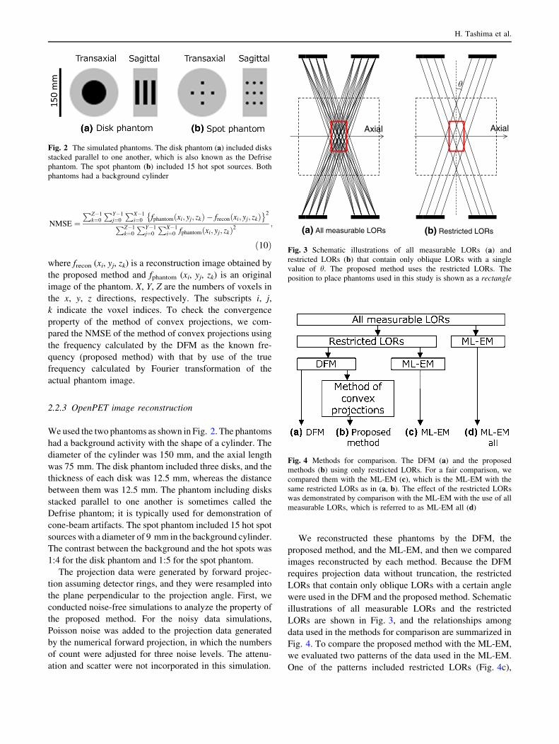
2.2.3 OpenPET image reconstruction

We used the two phantoms as shown in Fig. 2. The phantoms

had a background activity with the shape of a cylinder. The

diameter of the cylinder was 150 mm, and the axial length

was 75 mm. The disk phantom included three disks, and the

thickness of each disk was 12.5 mm, whereas the distance

between them was 12.5 mm. The phantom including disks

stacked parallel to one another is sometimes called the

Defrise phantom; it is typically used for demonstration of

cone-beam artifacts. The spot phantom included 15 hot spot

sources with a diameter of 9 mm in the background cylinder.

The contrast between the background and the hot spots was

1:4 for the disk phantom and 1:5 for the spot phantom.

The projection data were generated by forward projec-

tion assuming detector rings, and they were resampled into

the plane perpendicular to the projection angle. First, we

conducted noise-free simulations to analyze the property of

the proposed method. For the noisy data simulations,

Poisson noise was added to the projection data generated

by the numerical forward projection, in which the numbers

of count were adjusted for three noise levels. The attenu-

ation and scatter were not incorporated in this simulation.

We reconstructed these phantoms by the DFM, the

proposed method, and the ML-EM, and then we compared

images reconstructed by each method. Because the DFM

requires projection data without truncation, the restricted

LORs that contain only oblique LORs with a certain angle

were used in the DFM and the proposed method. Schematic

illustrations of all measurable LORs and the restricted

LORs are shown in Fig. 3, and the relationships among

data used in the methods for comparison are summarized in

Fig. 4. To compare the proposed method with the ML-EM,

we evaluated two patterns of the data used in the ML-EM.

One of the patterns included restricted LORs (Fig. 4c),

Fig. 2 The simulated phantoms. The disk phantom (a) included disks

stacked parallel to one another, which is also known as the Defrise

phantom. The spot phantom (b) included 15 hot spot sources. Both

phantoms had a background cylinder

Axial Axial

(a) All measurable LORs (b) Restricted LORs

Fig. 3 Schematic illustrations of all measurable LORs (a) and

restricted LORs (b) that contain only oblique LORs with a single

value of h. The proposed method uses the restricted LORs. The

position to place phantoms used in this study is shown as a rectangle

Fig. 4 Methods for comparison. The DFM (a) and the proposed

methods (b) using only restricted LORs. For a fair comparison, we

compared them with the ML-EM (c), which is the ML-EM with the

same restricted LORs as in (a, b). The effect of the restricted LORs

was demonstrated by comparison with the ML-EM with the use of all

measurable LORs, which is referred to as ML-EM all (d)

H. Tashima et al.

which was the same as for the proposed method, and the

other included all measurable LORs in the OpenPET

(Fig. 4d). The ML-EM with use of all measurable LORs is

hereinafter referred to as ML-EM all.

The reconstructed images were evaluated both in the

image domain and in the frequency domain by the 3D

Fourier transform. The error for the power spectra in the

two cone-shaped regions was calculated. As the error for

the power spectra, the mean squared error (MSE) was also

calculated to show the absolute amount of error in the

frequency domain:

MSE ¼XZ�1

k¼0

XY�1

j¼0

XX�1

i¼0

ffphantomðxi; yj; zkÞ � freconðxi; yj; zkÞg2

ð11Þ

To understand the effect of the constraint set used in the

proposed method, we changed the parameters for the object

support constraint. Also, the method of convex projections

with and without the non-negativity constraint was com-

pared. We applied the object support with diameters of

156, 188, 250, and 312 mm with and without the non-

negativity constraint. The reconstructed images with only

the non-negativity constraint were also calculated.

3 Results

3.1 Convergence of the proposed method

The relationships between the NMSE of the reconstructed

images and the number of iterations are shown in Fig. 5.

By about 3500 iterations for the disk phantom, the NMSE

of the proposed method decreased as the number of itera-

tions increased. However, starting from about 4000

iterations, the NMSE gradually diverged. In the case of the

spot phantom, the NMSE decreased rapidly and began to

diverge within 100 iterations. On the other hand, the

amounts of image updates, which are sums of absolute

differences between images fn-1 and fn, were converged.

We attribute this to errors in the calculation of the known

frequency by the DFM, such as the blurring effect in the

rebinning of the LOR data into the 2D projection image

and in the interpolation of the frequency components in the

Fourier domain. When we used the ideal frequency com-

ponents of the phantom which were calculated by Fourier

transformation of the actual phantom image (Fig. 6), the

NMSE did not diverge. Thus, we selected the images for

which the NMSE was at a minimum as the images for

Fig. 5 NMSE (left) and amount of image updates defined as the sum

of absolute differences (right) in the method of convex projections.

The result of the method of convex projections did not converge to the

ideal images due to the system errors such as interpolation error.

Arrows indicate minimum points. The amount of image updates

converged toward zero (right)

Fig. 6 NMSE in the method of convex projections using ideal

frequency components obtained by filtering of the Fourier transform

of the ideal images. The results of the method of convex projections

converge to the ideal images

Restoration of lost frequency in OpenPET imaging

comparison with the ML-EM. We note that the conver-

gence property when the projection data contained noise

was similar to the noise-free case.

3.2 OpenPET image reconstruction

The reconstruction images are shown in Fig. 7. The images

of Fig. 7a are the reconstruction images by the DFM,

which has the lost-frequency region in the Fourier domain.

The images of Fig. 7b are the reconstruction images by the

proposed method, which applied the method of convex

projection to the images reconstructed by the DFM. We

applied both a non-negativity and an object support con-

straint. The diameter for the object support constraint was

156 mm. The numbers of iterations for the method of

convex projections were 3500 for the disk phantom and 60

for the spot phantom. The images of Fig. 7c are the

reconstruction images by the ML-EM with use of restricted

LORs, the same as in the proposed method, and the images

of Fig. 7d were obtained by the ML-EM with use of all

measurable LORs (ML-EM all).

Because the image was reconstructed with incomplete

data, we needed more iterations than the usual ML-EM

image reconstruction. Therefore, we stopped the calcula-

tion of the ML-EM at 500 iterations. The calculation time

was measured on a workstation having two CPUs of 2.93-

GHz Intel� Xeon� X5570 and 12 GB memory. The cal-

culation time for the DFM was 3.3 s, and those for a single

iteration of the proposed method, the ML-EM, and the ML-

EM all were 0.47 s, 4.7 s, and 215 s, respectively. When

we applied only one constraint to the proposed method, the

calculation time for the single iteration was 0.44 s for the

object support constraint and was 0.45 s for the non-neg-

ativity constraint. We should note that the reconstruction

software was not optimized for high-speed computation,

and only a single thread was used. The profiles of the

reconstruction images of the disk phantom by each method

are shown in Fig. 8. These profiles were obtained along the

center line in each image.

As shown in Fig. 7a, the reconstruction images of the

disk phantom by the DFM had strong artifacts. The back-

ground between the disks disappeared. It can be seen from

Figs. 7b and 8 that artifacts in the reconstruction image of

the disk phantom were reduced by application of the

method of convex projections, and the disks were clearly

separated. On the other hand, the spot phantom could be

reconstructed by the DFM (Fig. 7a), and the influence of

the lost frequency on the spots was small.

In Fig. 7c, a ring artifact in the transaxial plane and a

streak artifact in the sagittal plane appeared in the ML-EM

reconstruction image. These artifacts were caused by the

sensitivity irregularity in the simulated OpenPET geome-

try, where the axial sampling in the simulated detector

rings and that in the image matrix were different. This

effect appeared strongly in the case of the MLEM with the

use of restricted LORs with only one oblique angle. In

Fig. 7 Reconstruction images

obtained with each method. The

center slices in each image are

shown. The profiles indicated by

horizontal lines in the disk

phantom images are plotted in

Fig. 8

H. Tashima et al.

addition, even if we use all measurable LORs for the ML-

EM all, there were still occurrences of artifacts and over-

estimation depending on the shape of the imaging subjects,

due to the incompleteness of the projection data.

Figure 9 shows the NMSE of the images reconstructed

by each method. The disk phantom contained larger errors

than did the spot phantom for every method. The proposed

method and ML-EM had a similar error for the disk

phantom. The NMSE of the spot phantom for the ML-EM

was much smaller than that for the proposed method. This

is because the components in the lost-frequency region

were small for the spot phantom; therefore, the effect of

restoration of the lost frequency was limited. Instead, the

effect of resampling from LORs for the detector rings to

the 2D projection data was dominant, whereas the ML-EM

has an advantage in which no rebinning is required.

Figure 10 shows vz - vy planes (vz = 0) of the power

spectra of the original phantom image and the reconstruc-

tion images. The two cone-shaped regions (Fig. 1b) in the

power spectrum of the reconstructed image by the DFM

were lost. The disk phantom contained many components

in the truncated regions compared with the spot phantom.

Therefore, the disk phantom was affected by the lost-fre-

quency components, whereas hot spots in the spot phantom

were well reconstructed in the case of DFM. The lost-

frequency components in the two cone-shaped regions

were restored by application of the method of convex

projections (Fig. 10c).

A similar tendency was observed in the case of ML-EM

(Fig. 10d, e). In Fig. 11, the NMSE and MSE were eval-

uated for the two cone-shaped regions in the power spec-

trum domain. In the spectrum domain, the NMSE of the

ML-EM restricted was almost the same as in the proposed

methods, whereas it was better in the image domain. The

ML-EM all had the best performance for both image and

power spectrum domains. For the spot phantom, the pro-

posed method could not restore the lost frequency in the

two cone-shaped regions well compared to ML-EM.

However, the amount of the lost-frequency component for

the spot phantom was much smaller than that for the disk

phantom. Actually, the MSE for the spot phantom was

small for all methods except for the DFM. Therefore, the

Fig. 8 The profiles of the reconstructed image of the disk phantom obtained by each method

Fig. 9 NMSE of the reconstructed images

Restoration of lost frequency in OpenPET imaging

difference in the restorative effect for the spot phantom was

not significant.

Figure 12 shows the effect of over-iterations with

100000 iterations. Components in the lost frequency tended

to be overestimated, and the resulting images suffered from

strong artifacts. Therefore, we needed to carefully choose

the optimum number of iterations, depending on the

imaging subject.

Figure 13 shows the effect of the constraint set used in

the proposed method. The numbers of iterations for each

result are shown in Table 2. The NMSE of each result is

plotted in Fig. 14.

The reconstructed images with non-negativity constraint

were almost the same for any diameter of the object sup-

port constraint. Without non-negativity constraint, how-

ever, the size of the object support constraint affected the

image quality. The NMSE convergence was much faster in

the case where the non-negativity constraint was applied

than in the case where only the object support constraint

was applied. In the case where the diameter for the object

support constraint was 188 mm, the NMSE of the disk

phantom did not reach a minimum even after 100000

Fig. 10 Original power spectrum of the disk phantom and reconstructed power spectra. The direction from left to right in the figures indicates

the axial direction (vz axis) in the Fourier domain. The vertical direction corresponds to the vy axis

Fig. 11 NMSE (left) and MSE (right) inside the two cone-shaped regions in the Fourier domain of the image reconstructed by each method

Fig. 12 Effect of over-iterations shown in the images reconstructed

by the proposed method after 100000 iterations. The constraints were

non-negativity and object support with a diameter of 156 mm

H. Tashima et al.

iterations, although the image updates for each step were

very small. Even so, the NMSE was the smallest when the

diameter for the object support constraint was almost the

same (156 mm) as the object background.

Figure 15 shows the images reconstructed from noisy

projection data with three different noise levels. The pro-

posed method could reduce the occurrence of the image

artifacts even in the noisy case, although slightly patchy

patterns appeared depending on the noise realizations.

Figure 16 shows the images reconstructed from noisy

projection data generated using different random seeds.

The results of the proposed method enhanced the noise in

the reconstructed images, and patchy patterns appeared.

The patterns were different from each other for different

noise realizations. The average image of the reconstructed

images from projection data with the 100 noise realizations

did not show the patchy pattern.

4 Discussion

The results for the disk phantom show that the method of

convex projections is effective in the restoration of the lost

frequency caused by the detector gap in OpenPET imaging.

In the case of the spot phantom, the spots could be

reconstructed well by the DFM (Fig. 7a). This is because

the spots consist mainly of high-frequency components

outside the lost-frequency region shown in Fig. 1b. Thus,

Fig. 13 Images restored by the

method of convex projections

with various constraints

Table 2 Optimum numbers of iterations for the method of convex

projections

Object support constraint (diameter) Optimum number of iterations

w/non-

negativity

constraint

w/o non-

negativity

constraint

Disk Spot Disk Spot

156 mm 3500 60 19400 7300

188 mm 3800 70 100000 42800

250 mm 4100 80 50400 37800

312 mm 4600 80 200 300

None 6300 100 N/A N/A

Fig. 14 NMSE of the images restored by the method of convex projections with various constraints

Restoration of lost frequency in OpenPET imaging

the spots are not sensitive to the lost frequency in OpenPET

imaging. The method of convex projections is effective

only at the edge of the background cylinder (Fig. 7b). From

Figs. 7, 8, 9, 10, 11, the results of the proposed method and

the ML-EM with use of restricted LORs show a tendency

similar to that of the proposed method. Therefore, the lost-

frequency restoration effects of these methods are nearly

equal. We consider that this is because the constraint set is

the same as or part of the constraints implicitly included in

the ML-EM.

Without non-negativity constraint, the NMSE was lower

than in the case where both constraints were applied only

when the object support diameter was almost the same as

the size of the background cylinder (Figs. 13, 14). This

indicates that the non-negativity constraint has a stronger

effect for image updates than did the object support.

However, due to the systematic error in the measurement

system, such as blurring and interpolation, the method of

convex projections did not converge toward the ideal

image, and we needed to stop the iteration when the NMSE

was optimal.

The imaging simulations with noisy data showed that

the proposed method was effective even when the number

of counts in the projection data was small while generating

a patchy pattern. However, the pattern disappeared by

averaging of multiple trials of the reconstruction of noisy

projection data generated using different random seeds

(Fig. 16). This means that the patchy pattern depends on

the initial noise pattern that appeared in the image recon-

structed by the DFM, and the method of convex projections

enhances it.

The object constraint also had the effect of improving

the image quality if it was set properly on the boundary of

the imaging object, whereas it had a weaker effect on

image updates than did the non-negativity constraint. In the

ML-EM, activities outside the object rapidly became zero

after a few iterations, and this is equivalent to the object

support constraint. Thus, the ML-EM implicitly applies the

same constraint set as does the proposed method.

The results reported in this paper show that the ML-EM

has the same lost-frequency restoration effect as does the

method of convex projections with the constraint set of

non-negativity and object support. Thus, iterative methods

which maximize the likelihood function are effective in

OpenPET imaging.

5 Conclusion

We proposed an analytical OpenPET image reconstruction

method that makes use of the method of convex projec-

tions, and we compared the proposed method with the ML-

Fig. 15 Images reconstructed

from noisy data by each

method. Constraints with non-

negativity and object support of

156 mm were applied for the

method of convex projections

with 3500 iterations for the disk

phantom and with 60 iterations

for the spot phantom. The

window level was set for each

noise level so that the maximum

value was equal to the count for

ideal hot disks

Fig. 16 Images reconstructed

by the DFM from different

noise realizations for the

projection data of about 5 M

counts (upper row), patchy

patterns appeared in the restored

images by the proposed method

(bottom row) and average image

of 100 noise realizations

(rightmost column)

H. Tashima et al.

EM in terms of the restorative effect on the lost frequency.

The results showed that the proposed method reduced the

image artifacts caused by the lost frequency. A tendency

similar to that for this restorative effect was observed in the

ML-EM image reconstruction, where no additional resto-

ration method was applied. Therefore, iterative image

reconstruction methods such as ML-EM involve the same

frequency restoration effect as does the method of convex

projections for the lost frequency caused by the detector

gap. We conclude that the iterative methods are effective in

OpenPET imaging.

Acknowledgments The authors would like to thank Dr. Shoko

Kinouchi for her support in developing simulation programs, and for

useful discussions. This work was supported in part by a Grant-in-Aid

for Japan Society for the Promotion of Science (JSPS) Fellows.

Conflict of interest The authors declare that they have no conflict

of interest.

References

1. Yamaya T, Inaniwa T, Minohara S, Yoshida E, Inadama N,

Nishikido F, et al. A proposal of an open PET geometry. Phys

Med Biol. 2008;53:757–73.

2. Yamaya T, Yoshida E, Inaniwa T, Sato S, Nakajima Y, Wakizaka

H, et al. Development of a small prototype for a proof-of-concept

of OpenPET imaging. Phys Med Biol. 2011;56:1123–37.

3. Yamaya T, Inaniwa T, Mori S, Furukawa T, Minohara S, Yoshida

E, et al. Imaging simulations of an ‘OpenPET’ geometry with

shifting detector rings. Radiol Phys Technol. 2008;2:62–9.

4. Yamaya T, Inaniwa T, Yoshida E, Nishikido F, Shibuya K, In-

adama N, et al. Simulation studies of a new ‘OpenPET’ geometry

based on a quad unit of detector rings. Phys Med Biol.

2009;54:1223–33.

5. Yamaya T, Yoshida E, Inadama N, et al. A multiplex ‘‘Open-

PET’’ geometry to extend axial FOV without increasing the

number of detectors. IEEE Trans Nucl Sci. 2009;56:2644–50.

6. Yoshida E, Yamaya T, Nishikido F, Inadama N, Murayama H.

Basic study of entire whole-body PET scanners based on the

OpenPET geometry. Nucl Instrum Methods Phys Res A.

2010;621:576–80.

7. Tashima H, Yoshida E, Kinouchi S, Nishikido F, Inadama N,

Murayama H, Suga M, Haneishi H, Yamaya T. Real-time

imaging system for the OpenPET. IEEE Trans Nucl Sci.

2012;59(1):40–6.

8. Iseki Y, Mizuno H, Futami Y, Tomitani T, Kanai T, Kanazawa

M, Kitagawa A, Murakami T, Nishio T, Suda M. Positron camera

for range verification of heavy-ion radiotherapy. Nucl Instrum

Methods Phys Res A. 2003;515:840–9.

9. Iseki Y, Kanai T, Kanazawa M, Kitagawa A, Mizuno H, Tomi-

tani T, et al. Range verification system using positron emitting

beams for heavy-ion radiotherapy. Phys Med Biol.

2004;49:3179–95.

10. Nishio T, Ogino T, Nomura K, Uchida H. Dose-volume delivery

guided proton therapy using beam on-line PET system. Med

Phys. 2006;33:4190–7.

11. Enghardt W, Crespo P, Fiedler F, Hinz R, Parodi K, Pawelke J,

et al. Charged hadron tumour therapy monitoring by means of

PET. Nucl Instrum Methods Phys Res A. 2004;525:284–8.

12. Crespo P, Shakirin G, Enghardt W. On the detector arrangement

for in-beam PET for hadron therapy monitoring. Phys Med Biol.

2006;51:2143–63.

13. Fiedler F, Shakirin G, Skowron J, Braess H, Crespo P, Kunath D,

et al. On the effectiveness of ion range determination from in-

beam PET data. Phys Med Biol. 2010;55:1989–98.

14. Inaniwa T, Kohno T, Tomitani T, et al. Experimental determi-

nation of particle range and dose distribution in thick targets

through fragmentation reactions of stable heavy ions. Phys Med

Biol. 2006;51:4129–46.

15. Tanaka E, Amo Y. A Fourier rebinning algorithm incorporating

spectral transfer efficiency for 3D PET. Phys Med Biol.

1998;43:739–46.

16. Orlov SS. Theory of three-dimensional reconstruction. 1. Con-

ditions for a complete set of projections. Soviet Phys Crystallogr.

1975;20:312–4.

17. Shepp LA, Vardi Y. Maximum likelihood reconstruction for

emission tomography. IEEE Trans Med Imag. 1982;MI-

1:113–22.

18. Hudson HM, Larkin RS. Accelerated image reconstruction using

ordered subsets of projection data. IEEE Trans Med Imag.

1994;13:601–9.

19. Youla DC, Webb H. Image restoration by the method of convex

projections: part 1—theory. IEEE Trans Med Imag. 1982;MI-

1:81–94.

20. Tuy H. Reconstruction of a three-dimensional object from limited

range of views. J Math Anal Appl. 1981;80:598–616.

21. Lent A, Tuy H. An iterative method for the extrapolation of band-

limited functions. J Math Anal Appl. 1981;83:554–65.

22. Kudo H, Saito T. Sinogram recovery with the method of convex

projections for limited-data reconstruction in computed tomog-

raphy. J Opt Soc Am A. 1991;8:1148–60.

23. Bendriem B, Townsend DW, editors. The theory and practice of

3D PET, Dordrecht. Netherlands: Kluwer Academic Publishers;

1998.

24. Tanaka E. Analytical methods of three-dimensional image

reconstruction. Med Imag Tech. 2000;18:33–9.

25. Sidky EY, Pan X. Image reconstruction in circular cone-beam

computed tomography by constrained, total-variation minimiza-

tion. Phys Med Biol. 2008;53:4777–807.

26. Knutsson HE, Edholm P, Granlund GH, Petersson CU. Ecto-

mography—a new radiographic reconstruction method—I. The-

ory and error estimates. IEEE Trans Biol Eng. 1980;27:640–8.

27. Dale S, Edholm PE, Hellstrom LG, Larsson S. Ectomography—a

tomographic method for gamma camera imaging. Phys Med Biol.

1985;30:1237–49.

Restoration of lost frequency in OpenPET imaging