8. 1

CHAPTER-8

RESULTS AND DISCUSSIONS

n this thesis, the concept of Quantum-inspired Evolutionary Algorithm (QIEA) is

initially presented along with its advantages over normal evolutionary algorithms.

Further, description of various types of soft computing techniques i.e. artificial neural

networks, neuro-fuzzy networks, genetic algorithms, simulated annealing algorithm,

evolutionary algorithms and hybrid evolutionary techniques and their detailed review

along with applications in optimization are presented.

An overview of quantum computation and its various concepts like hilbert space, bras

and kets, bits and qubits, bloch sphere, various quantum gates, quantum entanglement

and quantum parallelism are explained in detail.

A detailed review of Quantum-inspired Evolutionary Algorithms is discussed.

A review of FEM application in metal forming processes along with its use in forging

process modelling and design are discussed.

Severe plastic deformation and its different processing techniques are discussed while

giving Equal Channel Angular Pressing (ECAP) the main emphasis along with

detailed review.

8.1 Finite Element Modelling and Simulation of Hot Extrusion Process

Initially, flow formulation and deformation mechanics for the simulation and analysis

of metal forming process using FEM is presented. Further FEM based process

modelling is demonstrated. Mathematical formulation of metal forming processes is

discussed in detail.

A number of finite element simulations are performed for forward hot extrusion of a

preform for transmission shaft with various die angles (15o, 30o, 45o, 60o and 75o) at

temperatures varying from 1000oC to 1260oC using the finite element model. This

I

Chapter-8

8. 2

range of operating parameters is often used in industry for hot extrusion as per the

ASM specifications. The dies are kept at constant temperature (350oC). The 3

dimensional models of billet, lower die and upper die (punch) for simulation were

developed in solidworks software. The dies are assumed to be rigid pieces and the

billet material taken is ck-45 steel. Finite element simulation is done in FORGE3

environment.

The forging force or extrusion force at 50% reduction in diameter for few simulations

at 203 mm/s punch velocity and 1000oC with 0.4 co-efficient of friction is depicted

along with extrusion load graph with respect to displacement of upper die in figures

2.11, 2.12, 2.13, 2.14 and 2.15. The figures clearly indicate the evolution of extrusion

load with respect to punch travel and effect of die angle on the magnitude of extrusion

force.

Table 2.3 shows the FE simulation results for extrusion load required to extrude a

shaft by 50% reduction in its diameter with various die angles under different process

conditions at a punch velocity of 203 mm/sec.

The salient conclusions observed from the finite element simulations results as given

in table 2.3 are summarized below:

(i) Forging force or extrusion load reduces as the temperature of the billet

increases.

(ii) Forging force increases with increase in friction coefficient.

(iii) The forging force decreases with increase in die angle.

(iv) For die angle 75o the forging force increases in comparison with die angles 30o,

45o and 60o due to friction encountered in the conical shape pertaining to larger

die angle.

(v) The combination of process parameters i.e. temperature, velocity and die angle

and friction coefficient for minimum forging force needs an optimization

methodology to be applied in tandem with a new process model which can give

fast estimates of forging force unlike finite element model which requires

considerable time and effort.

Chapter-8

8. 3

The above conclusions can easily be visualized graphically by seeing the graphs in

figure 2.16 in which the effect on extrusion load for various die angles, coefficient of

friction and billet temperatures are shown.

As is to be expected the minimum extrusion force is for a combination of parameters

with maximum temperature, die angle and minimum friction coefficient. From a

practical point of view the high temperature can be obtained by appropriate heating,

the die angle can be selected as large as possible and the friction coefficient for a

billet - die material pair can be altered with suitable lubricant to some extent.

However, improper selection of the parameters may cause a folding defect in the billet

and inferior or defective parts.

8.2 Finite Element Modelling and Simulation of Equal Channel Angular Pressing(ECAP)

The 3D models for the ECAP simulation were developed in solidworks software with

the channel intersection angle Φ = 90° and angle of curvature Ψ = 0°. The dies are

assumed to be rigid pieces and the material used is an H13 tool-steel. The dimension

of the upper die or punch is 10mm (width) x 10mm (breadth) and 20mm (height). The

square shaped three dimensional workpiece (billet) considered has the dimensions of

10 mm (width) x 10 mm (breadth) and 60 mm (height) (refer figure 2.19). The

material of the billet is assumed to be Al 6061 aluminum alloy. Finite element

simulation is done in FORGE3 environment. It accurately predicts the material flow

and evolved equivalent strain during 3D bulk ECAP process. It enables fast

simulation of very complex and fully three-dimensional parts.

The FE modeling of ECAP process using Al 6061 billet is attempted for various

combinations of die channel angles (Φ = 90o, 105o and 120o), friction coefficient (μ =

0, 0.1, 0.15, 0.2, 0.25, 0.3, 0.35) and different processing routes, viz., Route A, Route

BA and Route C. Effect of these parameters on average equivalent strain in ECAPed

billet and forming energy required during ECAP process is studied and the results are

obtained by FE analysis.

Sample simulations illustrating isocontours of equivalent strain evolved during ECAP

process for channel angles (Φ =90o, 105o and 120o) after fourth pass of routes A, BA

Chapter-8

8. 4

and C are shown in figure 2.20, 2.21 and 2.22. Table 2.4 show results of FE

evaluation of average equivalent strain obtained in ECAPed billet and forming energy

(kJ) required during the ECAP process for various channel angles (Φ) after fourth

pass at various values of µ. Figure 2.23, 2.24 and 2.25 show graphs between average

equivalent strain and various coefficients of friction for different channel angles and

passes. Figures 2.26, 2.27 and 2.28 show graphs between average equivalent strain

and forming energy for different channel angles.

The salient conclusions observed from the finite element simulations results as given

in table 2.4 are summarized below:

i. The average equivalent strain imparted during ECAP is influenced mainly by

die channel angle (Φ).

ii. Channel angle of 90o imparts higher average equivalent strain in comparison

with those of 105o and 120o

iii. The forming energy required for Φ = 90o is more than that for 105o and 120o.

iv. Route A and BA imposes high average equivalent strain for all channel angles

in comparison with route C.

v. The average equivalent strain evolved during ECAP process increases with

number of passes and is maximum during fourth pass.

vi. The requirement of forming energy decreases with increase in number of

passes and is minimum during fourth pass.

8.3Neuro-fuzzy modelling of hot extrusion process and ECAP process

Neuro-fuzzy models have gained prominence on account of their flexibility to model

complex processes with experimental/simulation data. Their well-known model free

estimation makes them ideal candidate for fitness evaluation in the framework of

quantum evolutionary optimization.

Chapter-8

8. 5

8.3.1 Computational results of Neuro-fuzzy (NF) model for hot extrusion process

A neuro-fuzzy model is developed for hot extrusion process. The data obtained from

the FEM simulations of hot extrusion process; chapter-2, table 2.3 is used to train the

NF model. This model can be used to predict the extrusion forces for given parameter

combinations of hot extrusion in real-time without having to perform any extensive

and costly computations. A three input NF network is shown in figure 3.9. Neuro-

fuzzy inference system under consideration has three inputs viz. die angle (θ),

coefficient of friction (α) and initial temperature of billet (ν), and one output extrusion

load (f).

After developing the NF model from training it by FE simulation data the model is

validated. For this, the input parameters to the NF model are sets of values that have

not been used for training the model but are in the same range as those used for

training. This enables us to test the network with regard to its capability for

interpolation. The final extrusion force is thus obtained for this set of parameters.

Then an FE simulation is performed for the same sets of parameters to determine the

extrusion force. The level of agreement between the extrusion force predicted by NF

model and the FE simulation indicates the conformity of the NF model. The results of

the validation procedure described above are given in table 3.14. The close agreement

of the values of the final extrusion force obtained by the NF model and the FE

simulation clearly indicates that the model can be used for predicting the extrusion

force in the range of parameters under consideration. The model is very fast and

prediction can be done in real time.

8.3.2 Computational results of Neuro-fuzzy (NF) model for ECAP process

In this section, the neuro-fuzzy modelling of ECAP process is described. The data

obtained from the FEM simulations, Chapter 3, table 3.1 are used to train the NF

model. The neuro-fuzzy inference system under consideration has two inputs: channel

intersection angle (Φ) and coefficient of friction (µ) and two outputs: average

equivalent strain and forming energy (kJ). To achieve better accuracy in the results,

the prediction of average equivalent strain and forming energy are carried out

separately by two independent NF models in parallel as shown in figure 3.11. The

inputs are simultaneously fed to the two NF models and NF model-I fulfill the

Chapter-8

8. 6

prediction of the average equivalent strain, and NF model-II evaluates the forming

energy. As the two NF models are also trained separately, most suitable NF model

parameters could be found and thus better accuracy of prediction is attained. These

models can be used to predict the average equivalent strain and forming energy for

given parameter combinations of ECAP process in real-time without having to

perform any extensive and costly computations

The FE simulation results and NF estimated results for average equivalent strain and

forming energy are shown in table 3.15 and table 3.16 respectively. The close

agreement of simulated and trained values given by the developed neuro fuzzy model

clearly shows the efficacy of the model. The training information and the parameters

of NF architecture are shown in Table 3.17. The initial and final membership

functions for the NF model developed are shown in Fig. 3.14. The validation

procedure is same as discussed in section 9.3.1.

8.3.3 Neuro-fuzzy (NF) modelling of orthogonal cutting process

Cutting force estimation is an important criterion that determines the economics of

machining and is of engineering interest in intelligent manufacturing. A complex

relationship exists between process parameters like speed, feed, depth of cut, tool

geometry and cutting forces. There is a need to develop models that can capture this

interrelationship and enable fast computation of the cutting forces based on these

parameters. Here NF modelling of cutting forces for a given set of input parameters

i.e. speed, feed and depth of cut is attempted and the results obtained from NF model

compare favorably with the experimental data sets of cutting forces.

8.3.4 Neuro-fuzzy (NF) modelling of end milling process

The data obtained from the mentioned experimental setup in table 3.8, section 3.5 is

used to train the NF model for end milling process. The NF model is developed on

similar pattern as developed for forming processes in section 3.7 and 3.8. Neuro-fuzzy

inference system under consideration has four inputs as shown in figures 3.17 and

3.18 viz. cutting speed, feed rate, radial depth of cut, tolerance and one output

machining time and average surface roughness.

Chapter-8

8. 7

The experimental values reported by Tansel et al. [Tan06] and the computed values

after training NF model are listed in table 3.22. The close agreement of the values

obtained by the model and those reported by Tansel et al. clearly indicates that the

model can be used for predicting the values in the range of parameters under

consideration. The model is very fast and the time taken for prediction is negligible.

8.4 Regression modelling of manufacturing processes

8.4.1Regression modelling of hot extrusion process

Statistical regression model is developed using Minitab 15 for hot extrusion process

and is compared with NF model and FE model. Through the regression analysis of

the results, the values of the model coefficients have been obtained and the regression

equation for extrusion load as response is given as under:

Load = 405 – 0.562 Angle + 14.7 Friction – 0.135 Temp

The comparison of both the models i.e. NF model and Regression Analysis (RA)

model with FE modeled values in terms of relative percentage error for hot extrusion

process are shown in table 3.25. Error comparison of both the models is also shown

in table 3.26. Graph in fig. 3.20 shows comparison of FE modeled extrusion load

values and predicted values of NF and RA models.

The result of average percentage error (ϕa) is 0.33% for NF model as shown in table

3.26 for validation data set (n=6) and 9.54% for RA model. This means that the NF

model could predict the average equivalent strain with 99.67% accuracy as compared

to RA model with 90.46% accuracy. Further, R-squared (R2) and R-squared adjusted

(R2adj) values were also calculated which show the goodness of fit of the neuro-fuzzy

and regression models. For NF model the R2 value was 98.9% and R2adj was 99.1%.

For RA model the R2 value was 64.6% and R2adj was 62.7%. The NF model clearly

outperforms the statistical regression model.

8.4.2Regression modelling of ECAP process

The regression models for average equivalent strain and forming energy (kJ) of ECAP

process are also developed using Minitab 15 and are compared with NF model and FE

Chapter-8

8. 8

model. Through the regression analysis of the results, the values of the model

coefficients have been obtained and the regression equation for average equivalent

strain and forming energy are given as under:

Average Equivalent Strain = 17.7 - 0.125 angle + 3.07 friction

Forming Energy = 1.75 - 0.00583 angle + 0.763 friction

The result of average percentage error (ϕa) is 5.38% of average equivalent strain for

NF model as shown in table 3.28 for validation data set (n=9) and 20.42% for RA

model. This means that the NF model could predict the average equivalent strain with

94.62% accuracy as compared to RA model with just 79.58% accuracy. Further, R-

squared (R2) and R-squared adjusted (R2adj) values were also calculated which show

the goodness of fit of the neuro-fuzzy and regression models. For NF model the R2

value was 99.2% and R2adj was 99.6%. For RA model the R2 value was 97.9% and

R2adj was 97.7%.The results clearly shows that values of NF model are quite

consistent in comparison with RA modeled values.

The results shown in Table 3.29, 3.30 and Fig. 3.22 again clearly shows that values of

NF model are quite consistent in comparison with RA modeled values with those of

FE modeled values of forming energy for ECAP process. The result of average

percentage error (ϕa) is 3.56% of forming energy for NF model as shown in table 3.30

for validation data set (n=9) and 7.84% for RA model. This means that the NF model

could predict the forming energy with 96.44% accuracy as compared to RA model

with 92.16% accuracy. Further, R-squared (R2) and R-squared adjusted (R2adj) values

were also calculated which show the goodness of fit of the neuro-fuzzy and regression

models. For NF model the R2 value was 97.9% and R2adj was 98.2%. For RA model

the R2 value was 64.2% and R2adj was 60.8%. The NF model performance is again

found to be better than the statistical regression model.

8.4.3 Regression modelling of orthogonal cutting process

Through the regression analysis of the results, the values of the model coefficients

have been obtained and the regression equations of cutting forces (Ft and Fc) are given

as under:

Chapter-8

8. 9

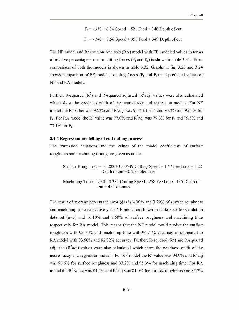
Ft = - 330 + 6.34 Speed + 521 Feed + 348 Depth of cut

Fc = - 343 + 7.56 Speed + 956 Feed + 349 Depth of cut

The NF model and Regression Analysis (RA) model with FE modeled values in terms

of relative percentage error for cutting forces (Ft and Fc) is shown in table 3.31. Error

comparison of both the models is shown in table 3.32. Graphs in fig. 3.23 and 3.24

shows comparison of FE modeled cutting forces (Ft and Fc) and predicted values of

NF and RA models.

Further, R-squared (R2) and R-squared adjusted (R2adj) values were also calculated

which show the goodness of fit of the neuro-fuzzy and regression models. For NF

model the R2 value was 92.3% and R2adj was 93.7% for Ft and 93.2% and 95.3% for

Fc. For RA model the R2 value was 77.0% and R2adj was 79.3% for Ft and 79.3% and

77.1% for Fc.

8.4.4 Regression modelling of end milling process

The regression equations and the values of the model coefficients of surface

roughness and machining timing are given as under.

Surface Roughness = - 0.288 + 0.00549 Cutting Speed + 1.47 Feed rate + 1.22 Depth of cut + 0.95 Tolerance

Machining Time = 99.0 - 0.235 Cutting Speed - 258 Feed rate - 135 Depth of cut + 46 Tolerance

The result of average percentage error (ϕa) is 4.06% and 3.29% of surface roughness

and machining time respectively for NF model as shown in table 3.35 for validation

data set (n=5) and 16.10% and 7.68% of surface roughness and machining time

respectively for RA model. This means that the NF model could predict the surface

roughness with 95.94% and machining time with 96.71% accuracy as compared to

RA model with 83.90% and 92.32% accuracy. Further, R-squared (R2) and R-squared

adjusted (R2adj) values were also calculated which show the goodness of fit of the

neuro-fuzzy and regression models. For NF model the R2 value was 94.9% and R2adj

was 96.6% for surface roughness and 93.2% and 95.3% for machining time. For RA

model the R2 value was 84.4% and R2adj was 81.0% for surface roughness and 87.7%

Chapter-8

8. 10

and 87% for machining time. The NF model clearly appears to outperform the

statistical regression model.

8.5 Development of Quantum Seeded Hybrid Evolutionary Computational Technique (QSHECT)

A general, flexible, and efficient Quantum Seeded Hybrid Evolutionary

Computational Technique (QSHECT) is developed which generates initial parents

using quantum seeds. It is here that QSHECT incorporates ideas from the principles

of quantum computation and integrates them in the current frame work of Real Coded

Evolutionary Algorithm (RCEA). The efficiency, effectiveness and ease of

application of the proposed technique are demonstrated by solving standard test bench

problems G1, G7, G9, G10 and engineering design problems such as gear design

problem, a truss design problem and a spring design problem. This technique also

incorporates Simulated Annealing (SA) in the selection process of Genetic Algorithm

(GA). It has been designed with genetic operator called the blend crossover (BLX) to

provide a better search capability. The algorithm is developed in MATLAB

environment.

The technique has been carefully designed with various features that enable it to seek

the global optimum rapidly without getting stuck in the local optima. It is clear from

the examples presented that QSHECT finds better solutions than the previously

known best optimal solutions. The algorithm allows a natural coding of design

variables by considering discrete/continuous variables. QSHECT finds a number of

solutions as an end results. Multiple optimal solutions can be simultaneously captured

with QSHECT. This gives designer more flexibility in optimization problems. The

results show a great promise in solving even system level design problems in future

with this new technique.

8.6 Development of Quantum Seeded Neuro Fuzzy Hybrid Evolutionary Computational Technique (QSNFHECT)

QSNFHECT uses neuro-fuzzy model in tandem with Quantum Seeded Hybrid

Evolutionary Computational Technique (QSHECT) for determining the optimal

process parameters. The methodology of QSNFHECT is shown in fig.5.1. The NF

Chapter-8

8. 11

model intelligently determines the output for a given set of input process parameters.

Once the NF model is ready it is incorporated in the QSHECT algorithm for fitness

evaluation while finding optimal values. This integration of NF model enables fast

computation of fitness function which is the primary requirement for successful

implementation of the evolutionary optimization.

8.6.1Result of QSNFHECT applied to hot extrusion process

The best solution i.e., optimum value of die angle, co-efficient of friction, die

velocity for minimum extrusion load obtained by QSNFHECT is shown in following

table 8.1. The optimal die angle and other process parameters obtained by

QSNFHECT are validated by the finite element model. Statistical information

obtained after 50 runs of QSNFHECT algorithm for hot extrusion process is also

obtained. QSNFHECT converged in 45 generations to optimal solution.

Optimaldie

angle (o)

Co-efficient of friction

()

Temp. of billet (oC)

Optimalextrusion load (tones)FEM result

QSNFHECT result

65 0.4 1260 218.71 220.13

Table 8.1: Final result of QSNFHECT indicating optimal process parameters and extrusion load with finite element validation for hot extrusion process.

8.6.2Result of QSNFHECT applied to ECAP process

The optimization of routes A, route BA and route C after fourth pass of ECAP process

is conducted using QSNFHECT algorithm methodology, to maximize average

equivalent strain and to minimize required forming energy. The results are further

validated by finite element model.

The optimum solutions i.e. optimum values of channel angle (ϕ) and coefficient of

friction (μ) for maximum predicted value of average equivalent strain and minimum

predicted value of forming energy is obtained in fifty runs by QSNFHECT algorithm

as shown in following table 8.2. Statistical information obtained after 50 runs of

QSNFHECT algorithm for different routes is also computed.

Chapter-8

8. 12

Route Results

Optimal Parameters

ChannelAngle

(ϕ)(o)

Co-efficient

of friction

()

Average Equivalent

Strain

ChannelAngle

(ϕ)(o)

Co-efficient

of friction

()

Forming Energy

(kJ)

AFEM 90 0.4 7.605 120 0.0 0.745

QSNFHECT 90 0.4 7.597 120 0.0 0.786

BAFEM 90 0.4 7.944 120 0.12 0.892

QSNFHECT 90 0.4 7.864 120 0.12 0.856

CFEM 90 0.4 7.188 120 0.0 0.795

QSNFHECT 90 0.4 7.203 120 0.0 0.821

Table 8.2: Final result of QSNFHECT indicating optimal average equivalent strain and forming energy with finite element validation of ECAP process

Following table 8.3 show number of generation taken by QSNFHECT for converging

the optimal values of average equivalent strain and forming energy for various routes.

Route Results Average Equivalent Strain Forming Energy (kJ)

No. of generations No. of generations

A QSNFHECT 52 40

BA QSNFHECT 47 43

C QSNFHECT 49 38

Table8.3: Number of generation taken by QSNFHECT for various routes

8.6.3Result of QSNFHECT applied to orthogonal cutting process

Orthogonal metal cutting is one of the most widely used processes in manufacturing.

The value of cutting speed, feed and depth of cut have significant effect on the

process optimization. Minimization of cutting forces with QSNFHECT algorithm

methodology is attempted in this work. Results obtained by QSNFHECT are shown

below in the table 8.4. The results are compared with those reported by Hans Raj et al.

The number of generations taken by QSNFHECT for computing optimal solution is

60 for both forces.

Chapter-8

8. 13

ForceCuttingspeed

FeedDepthof cut

Optimal valueof forces

(Hans Raj et al.)

Optimal valueof forces

(QSNFHECT)Fc 17.91 0.1070 1.01 230.48 228.39

Ft 17.61 0.1123 1.04 139.80 137.42

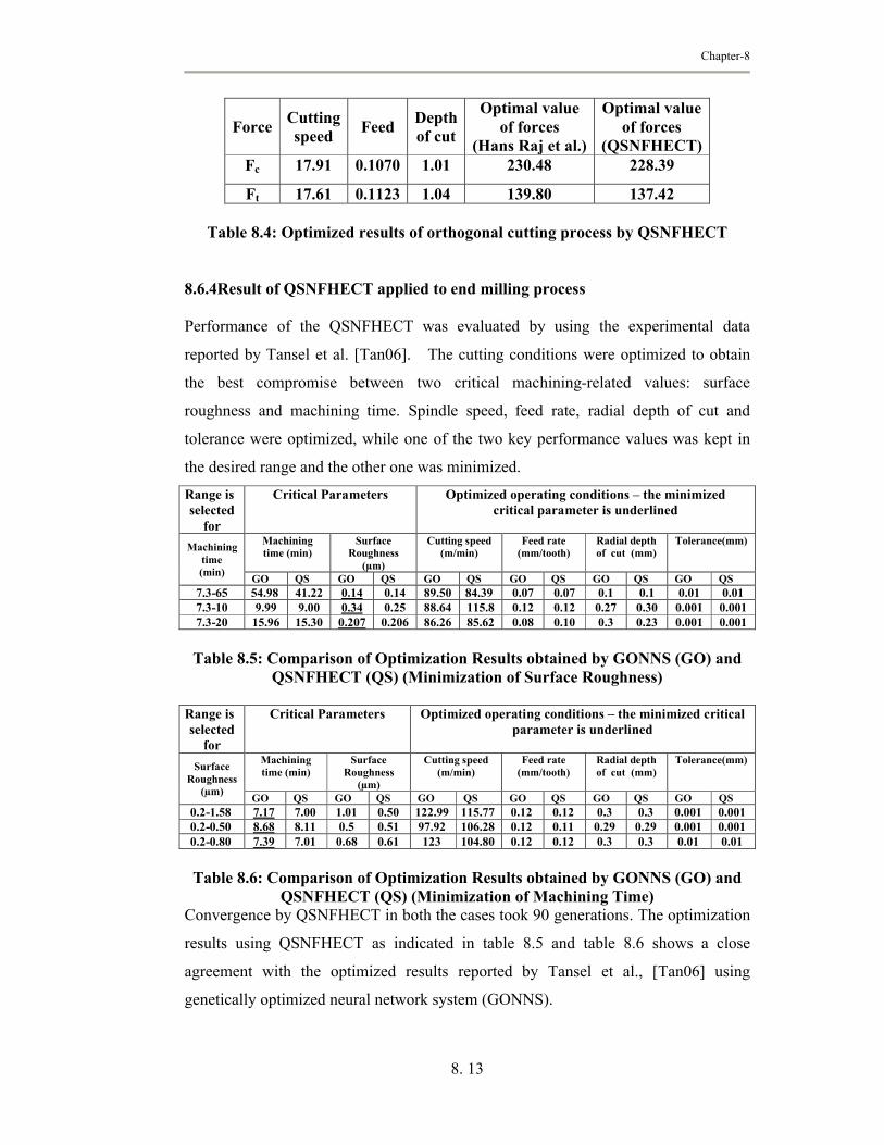
Table 8.4: Optimized results of orthogonal cutting process by QSNFHECT

8.6.4Result of QSNFHECT applied to end milling process

Performance of the QSNFHECT was evaluated by using the experimental data

reported by Tansel et al. [Tan06]. The cutting conditions were optimized to obtain

the best compromise between two critical machining-related values: surface

roughness and machining time. Spindle speed, feed rate, radial depth of cut and

tolerance were optimized, while one of the two key performance values was kept in

the desired range and the other one was minimized.

Range isselected

for

Critical Parameters Optimized operating conditions – the minimized critical parameter is underlined

Machining time (min)

Machining time (min)

Surface Roughness

(µm)

Cutting speed (m/min)

Feed rate (mm/tooth)

Radial depth of cut (mm)

Tolerance(mm)

GO QS GO QS GO QS GO QS GO QS GO QS7.3-65 54.98 41.22 0.14 0.14 89.50 84.39 0.07 0.07 0.1 0.1 0.01 0.017.3-10 9.99 9.00 0.34 0.25 88.64 115.8 0.12 0.12 0.27 0.30 0.001 0.0017.3-20 15.96 15.30 0.207 0.206 86.26 85.62 0.08 0.10 0.3 0.23 0.001 0.001

Table 8.5: Comparison of Optimization Results obtained by GONNS (GO) and QSNFHECT (QS) (Minimization of Surface Roughness)

Range isselected

for

Critical Parameters Optimized operating conditions – the minimized critical parameter is underlined

Surface Roughness

(µm)

Machining time (min)

Surface Roughness

(µm)

Cutting speed (m/min)

Feed rate (mm/tooth)

Radial depth of cut (mm)

Tolerance(mm)

GO QS GO QS GO QS GO QS GO QS GO QS0.2-1.58 7.17 7.00 1.01 0.50 122.99 115.77 0.12 0.12 0.3 0.3 0.001 0.0010.2-0.50 8.68 8.11 0.5 0.51 97.92 106.28 0.12 0.11 0.29 0.29 0.001 0.0010.2-0.80 7.39 7.01 0.68 0.61 123 104.80 0.12 0.12 0.3 0.3 0.01 0.01

Table 8.6: Comparison of Optimization Results obtained by GONNS (GO) and QSNFHECT (QS) (Minimization of Machining Time)

Convergence by QSNFHECT in both the cases took 90 generations. The optimization

results using QSNFHECT as indicated in table 8.5 and table 8.6 shows a close

agreement with the optimized results reported by Tansel et al., [Tan06] using

genetically optimized neural network system (GONNS).

Chapter-8

8. 14

The versatility of Quantum Seeded Neuro-Fuzzy Hybrid Evolutionary

Computational Technique (QSNFHECT) is demonstrated by applying it to different

manufacturing processes like hot extrusion, ECAP, orthogonal cutting and end milling

for the evaluation of final results. The QSNFHECT algorithm developed is modified

version of Quantum Seeded Hybrid Evolutionary Computational Technique

(QSHECT). In QSNFHECT a NF model is used to provide the fitness function value.

Thus QSNFHECT uses neuro-fuzzy network model in tandem with QSHECT in

determining the optimal process parameters. Results show that this is an innovative

approach for optimization of process parameters.

8.7 Development of Quantum-inspired Evolutionary Algorithm (QIEA) and its application to numerical optimization problems

Quantum-inspired Evolutionary Algorithm (QIEA) is a kind of evolutionary

algorithm where a qubit representation is adopted based on the concept and principles

of quantum computation. The major characteristic of the representation is that a linear

superposition of states can be represented. A classical bit is in one of two states, 0 or

1. A qubit also has a state, the two possible states of a qubit are 0 and 1 which

corresponds to the states 0 and 1 for a classical bit. These two states are known as

computational basis states. The difference between qubits and classical bits is that a

qubit may be in the ‘1’ state, in the ‘0’ state, or in any superposition of the two. The

state of a qubit can be represented as:

0 1

where α and β are complex numbers that specify the probability amplitudes of the

corresponding states. |α|2 gives the probability that the qubit will be found in the ‘0’

state and |β|2 gives the probability that the qubit will be found in the ‘1’ state.

In this work a real coded Quantum Inspired Evolutionary Algorithm (QIEA) is

developed and its effectiveness is demonstrated by solving six benchmark numerical

optimization problems with two different quantum gates, namely, rotation gate and Hε

gate. These gates are used to upgrade the quantum population and play a major role in

fast convergence and selection of best individual. The procedure of QIEA developed

in MATLAB environment.

Chapter-8

8. 15

The problems taken into consideration in this work are a set of six functions. These

functions are widely used as benchmark in numerical optimization. All these

functions are to be minimized. Function fsphere is unimodal and relatively easy to

minimize. Although fAckley is multimodal function but compared to other functions it is

not as difficult to optimize.

Other functions, fGriewank , fRastrigin , fschwefel and fRosenbrock are multimodal functions and

have lots of local minima, representing a harder class of functions to optimize. The

global minimum of all these functions is 0 except for fschwefel which has its global

minimum at f(x) = -418.9829n.

All the functions in the QIEA model were optimized for fifty experimental runs. The

population size for each function was taken to be 100. The termination condition with

the maximum number of generations was used.

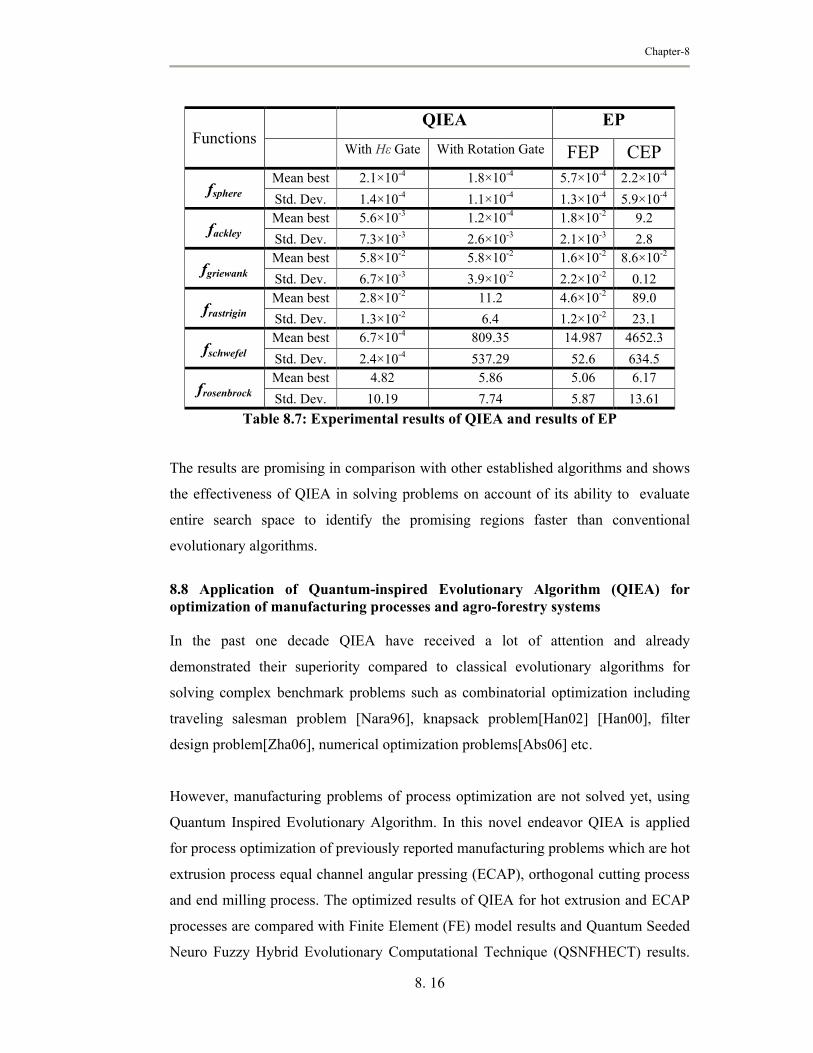
Experimental results with mean best solution and standard deviation of experimental

results for QIEA and the results of Evolutionary Programming (EP) are shown in

Table 8.7. The results of fsphere and fAckley with rotation gate are quite promising as

compared with Fast Evolutionary Programming (FEP) and Classical Evolutionary

Programming (CEP). This indicates that unimodal and relatively easy functions can

be best solved with rotation gate. In the case of fGriewank both the QIEAs, with rotation

gate and with Hε gate, gave the same results and are better than CEP although the

results of FEP are slightly better. In the cases of fRastrigin , fschwefel and fRosenbrock which

have many local minima, QIEA with Hε gate had significantly better results than

others. QIEA with rotation gate demonstrated better performance than CEP in these

cases.

Chapter-8

8. 16

Table 8.7: Experimental results of QIEA and results of EP

The results are promising in comparison with other established algorithms and shows

the effectiveness of QIEA in solving problems on account of its ability to evaluate

entire search space to identify the promising regions faster than conventional

evolutionary algorithms.

8.8 Application of Quantum-inspired Evolutionary Algorithm (QIEA) for optimization of manufacturing processes and agro-forestry systems

In the past one decade QIEA have received a lot of attention and already

demonstrated their superiority compared to classical evolutionary algorithms for

solving complex benchmark problems such as combinatorial optimization including

traveling salesman problem [Nara96], knapsack problem[Han02] [Han00], filter

design problem[Zha06], numerical optimization problems[Abs06] etc.

However, manufacturing problems of process optimization are not solved yet, using

Quantum Inspired Evolutionary Algorithm. In this novel endeavor QIEA is applied

for process optimization of previously reported manufacturing problems which are hot

extrusion process equal channel angular pressing (ECAP), orthogonal cutting process

and end milling process. The optimized results of QIEA for hot extrusion and ECAP

processes are compared with Finite Element (FE) model results and Quantum Seeded

Neuro Fuzzy Hybrid Evolutionary Computational Technique (QSNFHECT) results.

FunctionsQIEA EP

With Hε Gate With Rotation Gate FEP CEP

fsphereMean best 2.1×10-4 1.8×10-4 5.7×10-4 2.2×10-4

Std. Dev. 1.4×10-4 1.1×10-4 1.3×10-4 5.9×10-4

fackleyMean best 5.6×10-3 1.2×10-4 1.8×10-2 9.2

Std. Dev. 7.3×10-3 2.6×10-3 2.1×10-3 2.8

fgriewankMean best 5.8×10-2 5.8×10-2 1.6×10-2 8.6×10-2

Std. Dev. 6.7×10-3 3.9×10-2 2.2×10-2 0.12

frastriginMean best 2.8×10-2 11.2 4.6×10-2 89.0

Std. Dev. 1.3×10-2 6.4 1.2×10-2 23.1

fschwefelMean best 6.7×10-4 809.35 14.987 4652.3

Std. Dev. 2.4×10-4 537.29 52.6 634.5

frosenbrockMean best 4.82 5.86 5.06 6.17

Std. Dev. 10.19 7.74 5.87 13.61

Chapter-8

8. 17

For orthogonal cutting and end milling processes, optimized QIEA results are

compared with those reported in literature and QSNFHECT.

Further extending the application domain, QIEA for the very first time been applied

to optimize agro-forestry systems. Neuro-fuzzy modelling is conducted to predict the

yield of teak combined with agriculture crop from teak based agro-forestry systems.

kharif crops are modeled with QIEA as a constrained optimization problem with an

intent to maximize profit by allocating optimal land area to each individual crop.

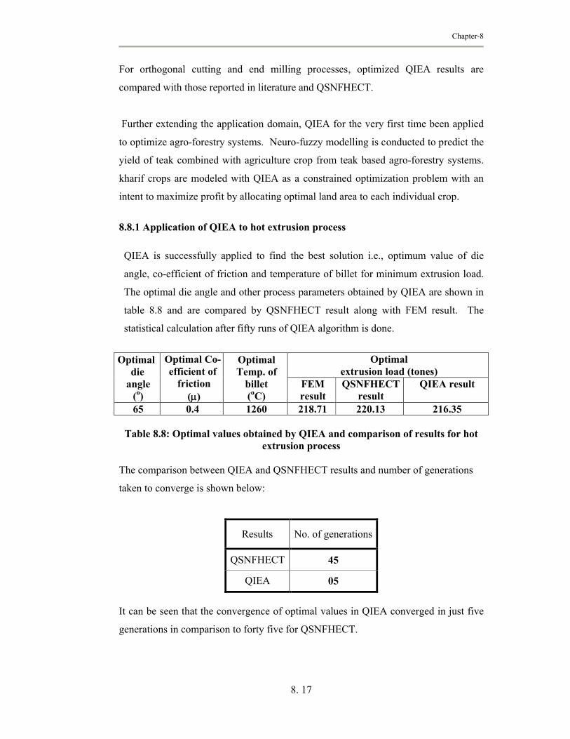
8.8.1 Application of QIEA to hot extrusion process

QIEA is successfully applied to find the best solution i.e., optimum value of die

angle, co-efficient of friction and temperature of billet for minimum extrusion load.

The optimal die angle and other process parameters obtained by QIEA are shown in

table 8.8 and are compared by QSNFHECT result along with FEM result. The

statistical calculation after fifty runs of QIEA algorithm is done.

Optimaldie

angle (o)

Optimal Co-efficient of

friction()

Optimal Temp. of

billet (oC)

Optimalextrusion load (tones)

FEM result

QSNFHECT result

QIEA result

65 0.4 1260 218.71 220.13 216.35

Table 8.8: Optimal values obtained by QIEA and comparison of results for hot extrusion process

The comparison between QIEA and QSNFHECT results and number of generations

taken to converge is shown below:

Results No. of generations

QSNFHECT 45

QIEA 05

It can be seen that the convergence of optimal values in QIEA converged in just five

generations in comparison to forty five for QSNFHECT.

Chapter-8

8. 18

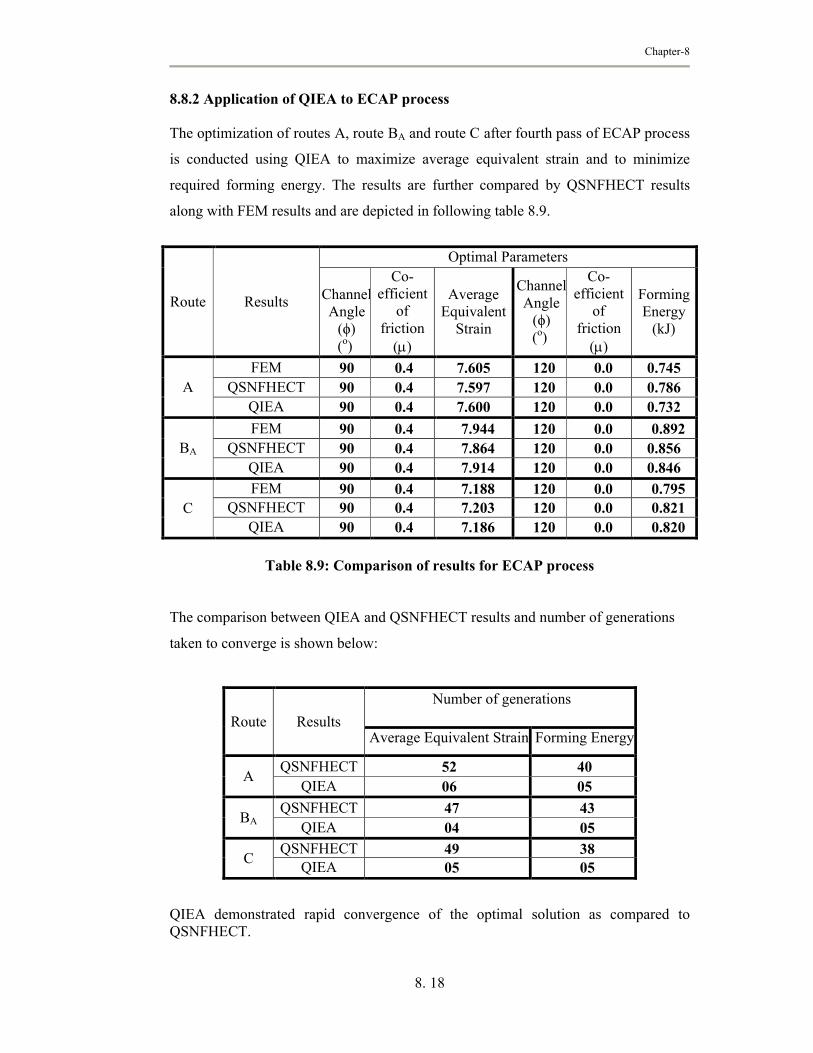
8.8.2 Application of QIEA to ECAP process

The optimization of routes A, route BA and route C after fourth pass of ECAP process

is conducted using QIEA to maximize average equivalent strain and to minimize

required forming energy. The results are further compared by QSNFHECT results

along with FEM results and are depicted in following table 8.9.

Route Results

Optimal Parameters

ChannelAngle

(ϕ)(o)

Co-efficient

of friction

()

Average Equivalent

Strain

ChannelAngle

(ϕ)(o)

Co-efficient

of friction

()

Forming Energy

(kJ)

AFEM 90 0.4 7.605 120 0.0 0.745

QSNFHECT 90 0.4 7.597 120 0.0 0.786QIEA 90 0.4 7.600 120 0.0 0.732

BA

FEM 90 0.4 7.944 120 0.0 0.892QSNFHECT 90 0.4 7.864 120 0.0 0.856

QIEA 90 0.4 7.914 120 0.0 0.846

CFEM 90 0.4 7.188 120 0.0 0.795

QSNFHECT 90 0.4 7.203 120 0.0 0.821QIEA 90 0.4 7.186 120 0.0 0.820

Table 8.9: Comparison of results for ECAP process

The comparison between QIEA and QSNFHECT results and number of generations

taken to converge is shown below:

Route Results

Number of generations

Average Equivalent Strain Forming Energy

AQSNFHECT 52 40

QIEA 06 05

BAQSNFHECT 47 43

QIEA 04 05

CQSNFHECT 49 38

QIEA 05 05

QIEA demonstrated rapid convergence of the optimal solution as compared to QSNFHECT.

Chapter-8

8. 19

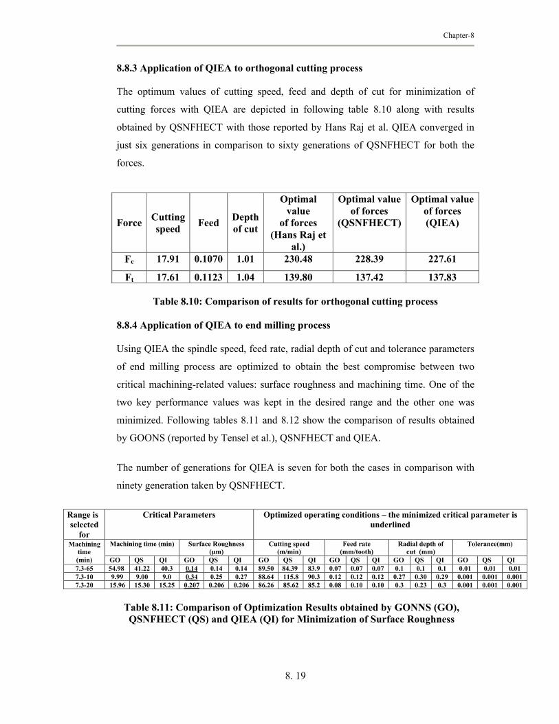
8.8.3 Application of QIEA to orthogonal cutting process

The optimum values of cutting speed, feed and depth of cut for minimization of

cutting forces with QIEA are depicted in following table 8.10 along with results

obtained by QSNFHECT with those reported by Hans Raj et al. QIEA converged in

just six generations in comparison to sixty generations of QSNFHECT for both the

forces.

ForceCuttingspeed

FeedDepthof cut

Optimal value

of forces(Hans Raj et

al.)

Optimal valueof forces

(QSNFHECT)

Optimal valueof forces(QIEA)

Fc 17.91 0.1070 1.01 230.48 228.39 227.61

Ft 17.61 0.1123 1.04 139.80 137.42 137.83

Table 8.10: Comparison of results for orthogonal cutting process

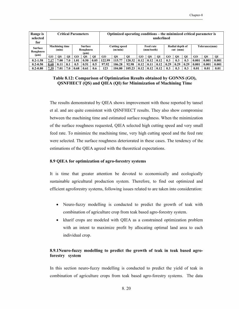
8.8.4 Application of QIEA to end milling process

Using QIEA the spindle speed, feed rate, radial depth of cut and tolerance parameters

of end milling process are optimized to obtain the best compromise between two

critical machining-related values: surface roughness and machining time. One of the

two key performance values was kept in the desired range and the other one was

minimized. Following tables 8.11 and 8.12 show the comparison of results obtained

by GOONS (reported by Tensel et al.), QSNFHECT and QIEA.

The number of generations for QIEA is seven for both the cases in comparison with

ninety generation taken by QSNFHECT.

Range isselected

for

Critical Parameters Optimized operating conditions – the minimized critical parameter is underlined

Machining time (min)

Machining time (min) Surface Roughness (µm)

Cutting speed (m/min)

Feed rate (mm/tooth)

Radial depth of cut (mm)

Tolerance(mm)

GO QS QI GO QS QI GO QS QI GO QS QI GO QS QI GO QS QI7.3-65 54.98 41.22 40.3 0.14 0.14 0.14 89.50 84.39 83.9 0.07 0.07 0.07 0.1 0.1 0.1 0.01 0.01 0.017.3-10 9.99 9.00 9.0 0.34 0.25 0.27 88.64 115.8 90.3 0.12 0.12 0.12 0.27 0.30 0.29 0.001 0.001 0.0017.3-20 15.96 15.30 15.25 0.207 0.206 0.206 86.26 85.62 85.2 0.08 0.10 0.10 0.3 0.23 0.3 0.001 0.001 0.001

Table 8.11: Comparison of Optimization Results obtained by GONNS (GO), QSNFHECT (QS) and QIEA (QI) for Minimization of Surface Roughness

Chapter-8

8. 20

Range isselected

for

Critical Parameters Optimized operating conditions – the minimized critical parameter is underlined

Surface Roughness

(µm)

Machining time (min)

Surface Roughness

(µm)

Cutting speed (m/min)

Feed rate (mm/tooth)

Radial depth of cut (mm)

Tolerance(mm)

GO QS QI GO QS QI GO QS QI GO QS QI GO QS QI GO QS QI0.2-1.58 7.17 7.00 7.0 1.01 0.50 0.05 122.99 115.77 120.32 0.12 0.12 0.12 0.3 0.3 0.3 0.001 0.001 0.0010.2-0.50 8.68 8.11 8.1 0.5 0.51 0.5 97.92 106.28 92.98 0.12 0.11 0.12 0.29 0.29 0.29 0.001 0.001 0.0010.2-0.80 7.39 7.01 7.0 0.68 0.61 0.6 123 104.80 105.23 0.12 0.12 0.12 0.3 0.3 0.3 0.01 0.01 0.01

Table 8.12: Comparison of Optimization Results obtained by GONNS (GO), QSNFHECT (QS) and QIEA (QI) for Minimization of Machining Time

The results demonstrated by QIEA shows improvement with those reported by tansel

et al. and are quite consistent with QSNFHECT results. They also show compromise

between the machining time and estimated surface roughness. When the minimization

of the surface roughness requested, QIEA selected high cutting speed and very small

feed rate. To minimize the machining time, very high cutting speed and the feed rate

were selected. The surface roughness deteriorated in these cases. The tendency of the

estimations of the QIEA agreed with the theoretical expectations.

8.9 QIEA for optimization of agro-forestry systems

It is time that greater attention be devoted to economically and ecologically

sustainable agricultural production system. Therefore, to find out optimized and

efficient agroforestry systems, following issues related to are taken into consideration:

Neuro-fuzzy modelling is conducted to predict the growth of teak with

combination of agriculture crop from teak based agro-forestry system.

kharif crops are modeled with QIEA as a constrained optimization problem

with an intent to maximize profit by allocating optimal land area to each

individual crop.

8.9.1Neuro-fuzzy modelling to predict the growth of teak in teak based agro-forestry system

In this section neuro-fuzzy modelling is conducted to predict the yield of teak in

combination of agriculture crops from teak based agro-forestry systems. The data

Chapter-8

8. 21

pertaining to yield of teak and associated agriculture crop like papaya, grass and

subabul at different spacing combinations viz., 10m and 20m spacing between two

rows of teak were collected by H. M. Chethana and reported in his M.S. thesis

submitted to University of Agricultural Sciences, Dharwad, Karnataka. The neuro-

fuzzy models are compared with regression models reported by H. M. Chethana. The

results clearly show the superiority of neuro-fuzzy models.

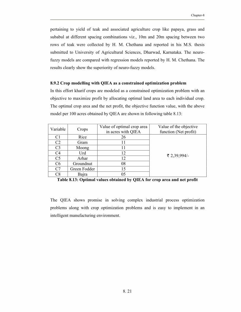
8.9.2 Crop modelling with QIEA as a constrained optimization problem

In this effort kharif crops are modeled as a constrained optimization problem with an

objective to maximize profit by allocating optimal land area to each individual crop.

The optimal crop area and the net profit, the objective function value, with the above

model per 100 acres obtained by QIEA are shown in following table 8.13:

Variable CropsValue of optimal crop area

in acres with QIEAValue of the objective function (Net profit)

C1 Rice 26

` 2,39,994/-

C2 Gram 11C3 Moong 11C4 Urd 12C5 Arhar 12C6 Groundnut 08C7 Green Fodder 15C8 Bajra 05Table 8.13: Optimal values obtained by QIEA for crop area and net profit

The QIEA shows promise in solving complex industrial process optimization

problems along with crop optimization problems and is easy to implement in an

intelligent manufacturing environment.