RESULTS OF THE DOWNHOLE MICROSEISMIC …gljpv/PDFS/Gajek_etal_2018.pdf · The first part of the paper (Gajek et al., 2018) introduces the experiment setting, geology and monitoring

RESULTS OF THE DOWNHOLE MICROSEISMIC MONITORING

AT A PILOT HYDRAULIC FRACTURING SITE IN POLAND,

PART II: SHEAR WAVE SPLITTING ANALYSIS

Journal: Interpretation

Manuscript ID INT-2017-0207.R2

Manuscript Type: 2017-05 Characterization of potential Lower Paleozoic shale resource play in Poland

Date Submitted by the Author: 28-May-2018

Complete List of Authors: Gajek, Wojciech; Polska Akademia Nauk Instytut Geofizyki, Department of Geophysical Imaging Malinowski, Michal; Institute of Geophysics PAS, Verdon, James; University of Bristol, School of Earth Sciences

Keywords: shear wave (S-wave), fractures, anisotropy, microseismic, shale gas

Subject Areas: Unconventional resources, Microseismic and monitoring of completion quality, Reservoir characterization/surveillance, Case studies

https://mc.manuscriptcentral.com/interpretation

Interpretation

This paper presented here as accepted for publication in Interpretation prior to copyediting and composition. © 2018 Society of Exploration Geophysicists and American Association of Petroleum Geologists.

Dow

nloa

ded

06/1

3/18

to 2

13.1

35.3

3.97

. Red

istr

ibut

ion

subj

ect t

o SE

G li

cens

e or

cop

yrig

ht; s

ee T

erm

s of

Use

at h

ttp://

libra

ry.s

eg.o

rg/

https://library.seg.org/action/showImage?doi=10.1190/int-2017-0207.1&iName=master.img-000.jpg&w=420&h=48



http://crossmark.crossref.org/dialog/?doi=10.1190%2Fint-2017-0207.1&domain=pdf&date_stamp=2018-06-08

PA

G

Interpretation

RESULTS OF THE DOWNHOLE MICROSEISMIC MONITORING AT A PILOT

HYDRAULIC FRACTURING SITE IN POLAND, PART II: SHEAR WAVE SPLITTING

ANALYSIS

Wojciech Gajek, Institute of Geophysics Polish Academy of Sciences, Warsaw, Poland,

E-mail: [email protected]

Michał Malinowski, Institute of Geophysics Polish Academy of Sciences, Warsaw,

Poland, E-mail: [email protected]

James P. Verdon, School of Earth Sciences, University of Bristol, Bristol, Great Britain,

E-mail: [email protected]

Original paper date of submission: ----

Revised paper date of submission: ----

Page 1 of 35


Interpretation

123456789101112131415161718192021222324252627282930313233343536373839404142434445464748495051525354555657585960


Dow

nloa

ded

06/1

3/18

to 2

13.1

35.3

3.97

. Red

istr

ibut

ion

subj

ect t

o SE

G li

cens

e or

cop

yrig

ht; s

ee T

erm

s of

Use

at h

ttp://

libra

ry.s

eg.o

rg/

PA

G

Interpretation

ABSTRACT

Observations of azimuthal seismic anisotropy provide useful information, notably on

stress orientation and the presence of pre-existing natural fracture systems, during hydraulic

fracturing operations. Seismic anisotropy can be observed through the measurement of shear-

wave splitting (SWS) on waveforms generated by microseismic events and recorded on

downhole geophone arrays. In this paper we present measurements of azimuthal anisotropy from

a Lower Paleozoic shale play in northern Poland. The observed orthorhombic anisotropic

symmetry system is dominated by a vertically-transverse isotropy (VTI) fabric, produced both by

the alignment of anisotropic platy clay minerals and by thin horizontal layering, and overprinted

by a weak azimuthal anisotropy. Despite the dominating VTI fabric, we successfully identify a

weaker HTI fabric striking east-southeast. We do this by constraining the rock-physics model

inversion with VTI background parameters incorporated from other geophysical methods:

microseismic velocity model inversion, 3D reflection seismic and borehole cross-dipole sonic

logs. The obtained orientation is consistent with a pre-existing natural fracture set that has been

observed using XRMI image logs from a nearby vertical well. The present-day regional

maximum horizontal stress direction differs from the observed fracture strike by approximately

45°. This implies that the SWS measurements recorded during hydraulic stimulation of shale gas

reservoir are imaging the pre-existing natural fracture set which influences the treatment

efficiency, instead of the present-day stress.

Page 2 of 35


Interpretation

123456789101112131415161718192021222324252627282930313233343536373839404142434445464748495051525354555657585960


Dow

nloa

ded

06/1

3/18

to 2

13.1

35.3

3.97

. Red

istr

ibut

ion

subj

ect t

o SE

G li

cens

e or

cop

yrig

ht; s

ee T

erm

s of

Use

at h

ttp://

libra

ry.s

eg.o

rg/

PA

G

Interpretation

INTRODUCTION

Most rocks display some degree of seismic anisotropy. There are numerous well-known

mechanisms causing anisotropy at various scales, including: preferred mineral or crystal

orientation (Johnston and Christensen, 1995; Lonardelli et al., 2007; Hall et al., 2008);

sedimentary layering (Backus, 1962; Liu and Martinez, 2012); aligned fracture sets (Hudson,

1981; Naar et al., 2006); and the application of anisotropic stresses (Lynn and Thomsen, 1986;

Verdon et al., 2008). One of the most direct indicators of anisotropy is a shear-wave splitting

(SWS), where a shear-wave propagating through anisotropic medium is split into two

orthogonally polarized shear-waves traveling with different velocities (Crampin et al., 1980;

Ando et al., 1980). The polarity of the fast and slow arrivals, and the delay times between the

two shear waves will be determined by the anisotropic symmetry system, and the direction of

wave propagation relative to this symmetry system. The delay time will also be determined by

the strength of the anisotropy (e.g. Verdon et al., 2009).

SWS has been exploited in various settings to retrieve important features of the

subsurface at various scales. It is observed in laboratory tests on stressed or fractured rocks (Nur

and Simmons, 1969; Xu and King; 1989, Ebrom et al., 1990, Tillotson et al., 2012), as well as in

global seismology for long-period waves propagating through the crust and mantle (e.g. Vinnik

at al., 1989; Silver and Chan, 1991; Savage, 1999). After being recognized as a useful

phenomenon at exploration scale (Crampin, 1985; Lynn and Thomsen, 1986; Willis et al., 1986),

SWS has been used in fracture detection from surface seismic (Martin and Davis, 1987; Mueller,

1991; Liu and Martinez, 2012), and multicomponent and walk-away VSP (Lynn et al., 1999;

MacBeth, 2002; Horne, 2003). SWS is also conventionally used in cross-dipole sonic logging for

Page 3 of 35


Interpretation

123456789101112131415161718192021222324252627282930313233343536373839404142434445464748495051525354555657585960


Dow

nloa

ded

06/1

3/18

to 2

13.1

35.3

3.97

. Red

istr

ibut

ion

subj

ect t

o SE

G li

cens

e or

cop

yrig

ht; s

ee T

erm

s of

Use

at h

ttp://

libra

ry.s

eg.o

rg/

PA

G

Interpretation

measuring in-situ azimuthal shear-wave anisotropy around the borehole (Mueller et al., 1994;

Patterson and Tang, 2001).

Two split shear modes are frequently observed during three-component downhole

microseismic monitoring in hydrocarbon reservoirs. This length scale is usefully positioned

between the lab scale and larger-scale seismic observations (Verdon and Wuestefeld, 2013).

Unlike VSP and reflection seismic imaging, measuring SWS with downhole receivers benefits

from the proximity of seismic sources (microearthquakes) and receiver arrays. Hence, it can be

efficiently used to image anisotropy within the reservoir without the overburden influence that

affects other methods (Wuestelfeld et al. 2011).

Measurements of seismic anisotropy from microseismicity can be used in a number of

ways, including: improving the accuracy of the velocity model (e.g., Grechka et al, 2011),

enhancing the precision of event locations (Grechka and Yaskevich, 2014), investigation of

fracture alignment (e.g., Miyazawa et al., 2008; Verdon and Kendall, 2011) and fracture

connectivity (e.g., Verdon and Wuestefeld, 2013; Baird et al., 2013); and determining changing

stress conditions generated by subsurface operations (e.g., Verdon et al., 2011). Measurements of

seismic anisotropy have been utilized in the geothermal industry (e.g. Rial et al., 2005) and for

carbon capture and storage (e.g. Verdon et al. 2011), although its most common application with

respect to microseismic data is during hydraulic fracturing of shale and tight gas reservoirs (e.g.,

Verdon and Wuestefeld, 2013).

The dominant symmetry system for many shales is a vertical-transverse isotropy (VTI)

fabric. In a VTI system, wave velocities are independent of azimuth, and depend solely on the

angle of ray propagation from vertical. VTI fabrics can be described by the Thomsen (1986)

Page 4 of 35


Interpretation

123456789101112131415161718192021222324252627282930313233343536373839404142434445464748495051525354555657585960


Dow

nloa

ded

06/1

3/18

to 2

13.1

35.3

3.97

. Red

istr

ibut

ion

subj

ect t

o SE

G li

cens

e or

cop

yrig

ht; s

ee T

erm

s of

Use

at h

ttp://

libra

ry.s

eg.o

rg/

PA

G

Interpretation

parameters ε, γ and δ under the weak anisotropy condition. In shales, this VTI system is

generated by the alignment of platy, anisotropic clay minerals within the sedimentary layers

(e.g., Kendall et al., 2007). Horizontal Transverse Isotropy (HTI) describes a medium when

velocity depends on the azimuth of propagation. HTI can be created by the presence of aligned

vertical fracture sets (Gupta, 1973; Crampin, 1985). Sedimentary rocks usually contain a

combination of VTI and HTI fabrics, creating orthorhombic symmetry (Tsvankin, 1997;

Grechka, 2007). In shales and mudstones the VTI fabric can be particularly strong, obscuring the

weaker effects of azimuthal anisotropy (e.g., Baird et al., 2018). As such, identifying the effects

of sedimentary fabrics to reveal the presence of fractures can be challenging.

In this paper we present a case study from the northern Poland Lower Paleozoic shale

play, where hydraulic stimulation was monitored using a downhole geophone array. We perform

SWS analysis to image the azimuthal anisotropy in the reservoir. The VTI fabric dominates over

the weaker azimuthal anisotropy and hinders the constraint of vertical fracture parameters during

an inversion of orthorhombic anisotropic model. However, by incorporating the VTI fabric

constrained by (i) 3D reflection seismic surveying, (ii) sonic log analysis and (iii) microseismic

event location analysis into our inversion procedure, we are able to obtain constrained

measurements of the azimuthal seismic anisotropy within the orthorhombic symmetry system.

The first part of the paper (Gajek et al., 2018) introduces the experiment setting, geology

and monitoring array geometry. It presents a VTI velocity model inversion based on recorded

perforation shots, location of microseismic events and hydraulic fracturing job effectiveness

assessment.

DATA AND METHODS

Page 5 of 35


Interpretation

123456789101112131415161718192021222324252627282930313233343536373839404142434445464748495051525354555657585960


Dow

nloa

ded

06/1

3/18

to 2

13.1

35.3

3.97

. Red

istr

ibut

ion

subj

ect t

o SE

G li

cens

e or

cop

yrig

ht; s

ee T

erm

s of

Use

at h

ttp://

libra

ry.s

eg.o

rg/

PA

G

Interpretation

In our case study, 6 stages of hydraulic fracturing were monitored using a 11-receiver

downhole geophone array located in vertical observation well near the heel of the horizontal

injection well. Example waveforms with both strong and weak SWS are shown in Figure 1. Most

of the recorded events had clear, strong SH-wave arrivals, and weaker P-wave arrivals. SWS was

visible on the majority of records – at least 1/3 of the events had clear SV-wave onsets. A

detailed description of the site, geometry, data processing and VTI model inversion can be found

in Gajek et al., (2018). The anisotropy is manifested by a significant, stage-varying S-wave

splitting (up to 40 ms for some of the events), necessitating the use of an anisotropic velocity

model for the purpose of microseismic event location. A 1D, 5-layer VTI model was built using

travel-times from 13 perforation shots and selected microseismic events. The model consisted of

layer-dependent velocities and effective Thomsen’s parameters for all the layers. Finally,

detected events were located by inverting picked travel times, using a Bayesian approach (e.g.,

Tarantola, 2005; Gajek et al., 2016).

SWS measurements provide the polarization (Φ) of the fast shear wave, and the time

delay (dt) between the two split shear modes (Wolfe and Silver, 1999; Teanby et al., 2004). A

measurement can be made for each source-receiver pair, resulting in considerable amount of data

when geophone array is used to record hundreds of events. To deal the large number of

measurements thus required, we use the automated method described by Wuestefeld et al.

(2010), which is based in turn on that described by Teanby et al. (2004). The workflow is

presented in Figure 2. Recorded waveforms are rotated to the ray-frame coordinates in order to

minimise P-wave energy on the qSH and qSV components. Next, the SWS correction is applied,

resulting in a linearization of the particle motion in fast- and slow-axes coordinate system

(Figure 2c). The SWS correction is determined by applying all possible fast S-wave orientations

Page 6 of 35


Interpretation

123456789101112131415161718192021222324252627282930313233343536373839404142434445464748495051525354555657585960


Dow

nloa

ded

06/1

3/18

to 2

13.1

35.3

3.97

. Red

istr

ibut

ion

subj

ect t

o SE

G li

cens

e or

cop

yrig

ht; s

ee T

erm

s of

Use

at h

ttp://

libra

ry.s

eg.o

rg/

PA

G

Interpretation

and time shifts and then retrieving the minimum error solution from resulting error surface

(Figure 2d). The analysis is performed for various-length S-wave windows to provide a stable

solution regardless of window position and length (Figure 2e). A more detailed description of

this workflow is described in the Figure 2 caption.

To ensure good data quality, the acceptance criteria defined by Teanby et al. (2004) were

used to ensure that only robust SWS measurements were taken forward for further analysis

including:

1. good event signal-to-noise ratio;

2. linear P-wave motion allowing a well-constrained rotation from geographical (N-

E-Z) to ray-frame (qP-qSH-qSV) coordinate system;

3. effective minimisation of energy on the transverse component after the SWS

correction has been applied, resulting in linear post-correction particle motion,

and matching post-correction waveforms in a fast- and slow-S-wave coordinate

system;

4. a single, tightly constrained minimum in the error surface;

5. consistent SWS results regardless of the choice of the analysis window start time

and length.

A good quality result must fulfil all of these conditions. These criteria were first assessed

automatically by discarding results which evidently neglected any of these conditions. Then

Page 7 of 35


Interpretation

123456789101112131415161718192021222324252627282930313233343536373839404142434445464748495051525354555657585960


Dow

nloa

ded

06/1

3/18

to 2

13.1

35.3

3.97

. Red

istr

ibut

ion

subj

ect t

o SE

G li

cens

e or

cop

yrig

ht; s

ee T

erm

s of

Use

at h

ttp://

libra

ry.s

eg.o

rg/

PA

G

Interpretation

remaining SWS measurements were assessed manually via the inspection of figures such as that

shown in Figure 2.

INVERSION OF SWS MEASUREMENTS FOR ROCK PHYSICS PARAMETERS

A single measurement of dt and Φ along a single raypath is not sufficient to constrain the

overall anisotropic symmetry system. Instead, a population of SWS measurements along a range

of raypaths must be inverted to reveal the overall anisotropy. Typically, a rock-physics model,

assuming a particular anisotropic symmetry system, must be created, which is then compared to

the observations, with the best-fitting rock physics model parameterisation being taken as the

result (e.g., Verdon et al., 2009).

In this case we inverted measured fast polarization angles and time delays for a

background VTI fabric (Thomsen, 2002) overprinted with a single set of vertically aligned,

unfilled, penny-shaped fractures (Hudson, 1981), resulting in effective orthorhombic symmetry.

The inversion is resolved for four free parameters of the effective orthorhombic medium between

receivers and microseismic sources:

• the fracture density ξ and strike α of the vertical fracture set,

• Thomsen’s parameters describing the VTI rock fabric,

• with only S-wave data, δ and ε cannot be constrained independently, instead a

ratio between δ and ε is resolved.

The inversion is performed following the method described by Verdon et al. (2009) and Verdon

and Wuestefeld (2013). When iterating over a parameter space (ξ, α, δ and γ), the elastic stiffness

Page 8 of 35


Interpretation

123456789101112131415161718192021222324252627282930313233343536373839404142434445464748495051525354555657585960


Dow

nloa

ded

06/1

3/18

to 2

13.1

35.3

3.97

. Red

istr

ibut

ion

subj

ect t

o SE

G li

cens

e or

cop

yrig

ht; s

ee T

erm

s of

Use

at h

ttp://

libra

ry.s

eg.o

rg/

PA

G

Interpretation

tensor providing velocities and polarizations of S-waves for any direction is computed by solving

a Christoffel equation, independent from Thomsen’s weak anisotropy assumption (Thomsen,

1986). The background P- and S-wave velocities, VP0, VS0, and density are held constant

through the model space. Velocities are based on the VTI velocity model described by Gajek et

al. (2018), while mean density was taken from the well-log interval of interest.

RESULTS

Out of over 14,000 SWS measurements, 561 were accepted as good quality results under

our strict acceptance criteria. The spatial distribution of microseismic events with a good quality

measurement on at least one trace is plotted in Figure 3 as a map view and in Figure 4 as a side

view. Significant noise levels restricted the number of good measurements, especially for distant

stages: only 4% of accepted measurements belonged to stages 1 – 3 (the most distant from the

observation well). The accepted measurements had ca. 35° wide azimuthal coverage and 35-70°

incidence angles coverage (Figure 5a,b). The majority of fast shear-wave polarization angles are

at 90° relative to the qSV orientation, i.e. they are near-horizontal, as expected from a VTI

system. However, significant numbers of events do not have horizontal fast shear-wave

polarisations, and indeed the delay times for these events are often larger than the delay times for

those with horizontal polarisations (Figure 5c). These observations imply that the system is not

solely VTI. Instead, such a signature can be recognized as VTI fabric influenced by vertical

fractures (Usher et al, 2015).

The inversion of SWS measurements for an orthorhombic rock physics model without

any prior VTI fabric constraints resulted in unstable fracture parameters (strike α and crack

density ξ). Those parameters were not constrained because the relatively weaker azimuthal

Page 9 of 35


Interpretation

123456789101112131415161718192021222324252627282930313233343536373839404142434445464748495051525354555657585960


Dow

nloa

ded

06/1

3/18

to 2

13.1

35.3

3.97

. Red

istr

ibut

ion

subj

ect t

o SE

G li

cens

e or

cop

yrig

ht; s

ee T

erm

s of

Use

at h

ttp://

libra

ry.s

eg.o

rg/

PA

G

Interpretation

anisotropy did not contribute significantly to the overall model due to limited azimuthal and

incidence angle data coverage (Verdon et al., 2009) and stronger VTI fabric that dominates the

inversion (Gajek et al., 2017).

However, the VTI fabric has already been observed by other geophysical methods,

including (i) 3D VTI pre-stack depth migration velocity model (Kowalski et al. 2014) from a

coincident 3D seismic survey, for which γ was derived using empirical relation to ε (Wang,

2001), (ii) Backus-averaged well-logs, (iii) the velocity model inverted for microseismic event

location, described by Gajek et al., (2018). Sonic, density and natural gamma logs were used to

obtain the vertical velocities Vp0 and Vs0, and to derive Thomsen’s parameters (Thomsen,

1986). Those parameters were downscaled to 200 Hz using a Backus-averaging scheme (Backus,

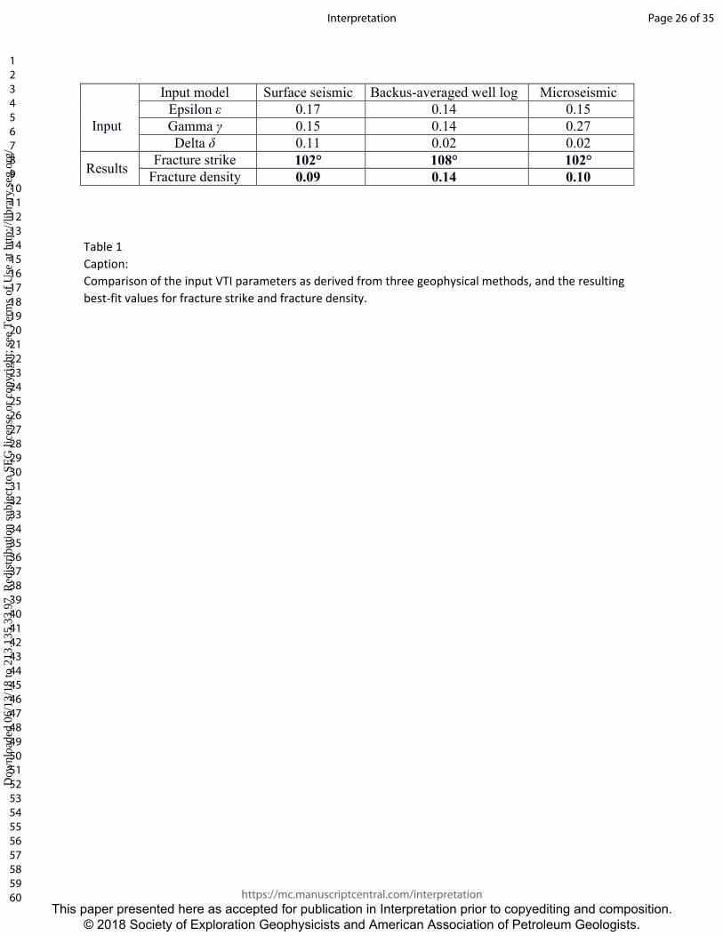
1962). The VTI parameters for three models are listed in Table 1. There is some disagreement

between the prior VTI measurements. We therefore explored the effect on the fracture

parameters (α and ξ) inverted from SWS measurements when the VTI fabric is fixed, doing this

using each of the VTI fabrics determined from each of the geophysical methods (reflection

seismic, well-log, microseismic). The results are listed in Table 1.

We find that, within the range of possible VTI parameters defined by the seismic, well

log and microseismic observations, then inversion for fracture strikes and densities are well

constrained and consistent, ranging between 102 - 108 degrees and 0.09 – 0.14, respectively

(Figure 6).

DISCUSSION

Page 10 of 35


Interpretation

123456789101112131415161718192021222324252627282930313233343536373839404142434445464748495051525354555657585960


Dow

nloa

ded

06/1

3/18

to 2

13.1

35.3

3.97

. Red

istr

ibut

ion

subj

ect t

o SE

G li

cens

e or

cop

yrig

ht; s

ee T

erm

s of

Use

at h

ttp://

libra

ry.s

eg.o

rg/

PA

G

Interpretation

We assumed a VTI medium influenced by vertical cracks after judging from S-wave

delay times and corresponding incidence angle (Figure 5c). However, for particular solely VTI

settings the SV-wave can propagate faster than SH-wave towards particular directions (Thomsen,

1986). Nevertheless, we excluded this possibility basing on a synthetic model of SH- and SV-

wave velocities in VTI medium (Figure 7). Two scenarios for the strongest (γ=0.27) and the

weakest (γ=0.14) anisotropy among finally obtained models (Table 1) were tested, with common

parameters: Vs0=2400 m/s, ε=0.15, δ=0.02. For this particular VTI media the SV-wave can be

slightly faster than SH-wave in case of the lower anisotropy scenario. However, in the range of

incidence angled sampled by SWS measurements SH-wave velocity prevails, hence, the

assumption of VTI fabric with vertical cracks remains valid.

The observation well is close to the heel of the injection well, while the fracturing stages

proceeded from the toe to the heel, as is common practice during hydraulic fracturing operations.

Such geometry promotes the influence of final stages of the stimulation by limiting the amount

of events from initial stages due to the S/N decay with the distance (Figure 4). What’s more, it

limits the available azimuthal coverage of splitting measurements where maximum azimuthal

span is provided mostly by events within the closest, i.e. final stages (Figure 3). Consequently,

the unconstrained inversion of rock-physics parameters did not produce a stable result.

The inversion became well-resolved after fixing the model’s VTI parameters. The

geophysical data sources used to constrain the inversion vary significantly in scale from seismic

frequencies, through microseismic frequencies and up to sonic logs (downscaled to 200 Hz by

Backus averaging (Backus, 1962)). Nevertheless, the obtained fractures strike and fracture

density were constrained well for all three models (Figure 8).

Page 11 of 35


Interpretation

123456789101112131415161718192021222324252627282930313233343536373839404142434445464748495051525354555657585960


Dow

nloa

ded

06/1

3/18

to 2

13.1

35.3

3.97

. Red

istr

ibut

ion

subj

ect t

o SE

G li

cens

e or

cop

yrig

ht; s

ee T

erm

s of

Use

at h

ttp://

libra

ry.s

eg.o

rg/

PA

G

Interpretation

The fracture strike of 102-108° obtained using SWS data is close to the ca. 125° strike of

the J2 fracture set obtained from XRMI log interpretation presented in Figure 9 (Bobek and

Jarosiński, 2018). The J2 set has biggest contribution to the interval influencing SWS

measurements and dominates in the Sasino formation (see Figure 7b in Gajek et al., 2018). It

also contributes to the azimuthal anisotropy as detected by 3D wide-azimuth P-wave seismic

data, where similar fracture strikes were inferred (Cyz and Malinowski, 2018). Estimated

fracture strike can be influenced by a secondary fracture set J’ striking approximately 80°,

however, trying to invert for two fracture sets did not result in any stable strike of second fracture

set.

The imaged direction differs by 45-50° from the in-situ regional maximum horizontal

stress orientation, which has an azimuth ca. 155° (Jarosiński, 2005). This indicates that the SWS

measurements are imaging pre-existing natural fractures rather than new fractures created during

stimulation, which would be expected to strike parallel to the maximum horizontal stress.

However, this is to be expected when the geometry of observation and injection wells is

considered: the ray paths from each of the stages are predominantly through the un-stimulated

rock ahead (i.e. “heel-wards”) of the stimulation stages, and therefore can only image the pre-

existing natural fractures.

Baird et al. (2013) showed how the anisotropic system can change as hydraulic fracturing

proceeds and ray-paths switch from propagation through unstimulated rock to rocks that have

been stimulated, resulting in a change in the dominant fracture strike from that of the pre-existing

fractures to that of the present day maximum horizontal stress direction (and the presumed

orientation of the hydraulic fractures). Baird et al. (2013) also noted an increase in the fracture

Page 12 of 35


Interpretation

123456789101112131415161718192021222324252627282930313233343536373839404142434445464748495051525354555657585960


Dow

nloa

ded

06/1

3/18

to 2

13.1

35.3

3.97

. Red

istr

ibut

ion

subj

ect t

o SE

G li

cens

e or

cop

yrig

ht; s

ee T

erm

s of

Use

at h

ttp://

libra

ry.s

eg.o

rg/

PA

G

Interpretation

compliance ratio (ZN/ZT) representing the change from partially filled and poorly-connected old

fractures to the “clean”, well-connected new hydraulic fractures. To replicate such

measurements, ray-paths through the already-stimulated volumes are required, which in turn

would require an observation well at the toe end of the injection well for this particular well

configuration.

CONCLUSIONS

We have performed SWS analysis in order to invert for fracture parameters during the

pilot hydraulic stimulation of the Lower Paleozoic shale target located in Northern Poland. The

stimulated shale displays orthorhombic anisotropy with dominant VTI fabric overprinted by

weaker azimuthal anisotropy. The imprint of the VTI fabric makes the inversion for fracture

parameters harder than it otherwise would be. However, by incorporating constraints on VTI

parameters from other geophysical measurements, we are able to invert the observed SWS

measurements for a well-constrained estimate of fracture strike of 102 – 108° and fracture

density of 0.09 – 0.14. The resulting fracture strike corresponds to the orientation of pre-existing

fractures obtained from XRMI log, and from the analysis of the surface seismic data, but is

different from the fracture orientation expected from hydraulic fracturing based on the regional

maximum horizontal stress direction.

ACKNOWLEDGMENTS

This research was conducted within the ShaleMech project funded by the Polish National

Centre for Research and Development (NCBR), grant no. BG2/SHALEMECH/14. Data were

provided by the PGNiG SA. Collaboration with University of Bristol was supported within

Page 13 of 35


Interpretation

123456789101112131415161718192021222324252627282930313233343536373839404142434445464748495051525354555657585960


Dow

nloa

ded

06/1

3/18

to 2

13.1

35.3

3.97

. Red

istr

ibut

ion

subj

ect t

o SE

G li

cens

e or

cop

yrig

ht; s

ee T

erm

s of

Use

at h

ttp://

libra

ry.s

eg.o

rg/

PA

G

Interpretation

TIDES COST Action ES1401. XRMI and cross-dipole sonic interpretation was performed by the

Institute of Oil and Gas – National Research Institute. We thank the Associate Editor, Dr

Andrzej Pasternacki, as well as the anonymous reviewers for their useful comments.

REFERENCES

Ando, M., Ishikawa, Y., and Wada, H., 1980, S-wave anisotropy in the upper mantle under a

volcanic area in Japan: Nature 286, 43–46.

Backus, G.E., 1962, Long-wave elastic anisotropy produced by horizontal layering: J. Geophys.

Res., 66, 4427–4440.

Baird, A. F., Kendall, J. M., Verdon, J. P., Wuestefeld, A., Noble, T. E., Li, Y., Dutko, M., and

Fisher, Q. J., 2013, Monitoring increases in fracture connectivity during hydraulic

stimulations from temporal variations in shear wave splitting polarization: Geophysi J Int,

195(2), 1120-1131.

Baird, A.F., Kendall, J-M., Fisher, Q.J., and Budge, J., 2018, The role of texture, cracks and

fractures in highly anisotropic shales: submitted to Journal of Geophysical Research, in

review.

Bobek, K., and Jarosiński, M., 2018, Parallel structural interpretation of drill cores and

microresistivity scanner images from gas-bearing shale (Baltic Basin, Poland),

Interpretation, this volume (in review).

Page 14 of 35


Interpretation

123456789101112131415161718192021222324252627282930313233343536373839404142434445464748495051525354555657585960


Dow

nloa

ded

06/1

3/18

to 2

13.1

35.3

3.97

. Red

istr

ibut

ion

subj

ect t

o SE

G li

cens

e or

cop

yrig

ht; s

ee T

erm

s of

Use

at h

ttp://

libra

ry.s

eg.o

rg/

https://library.seg.org/action/showLinks?doi=10.1190%2Fint-2017-0207.1&isi=A1980JX86000033&citationId=p_1

PA

G

Interpretation

Crampin, S., Evans, R., Üçer, B., Doyle, M, Davis, J. P.,Yegorkina, G. B., and Miller, A., 1980,

Observations of dilatancy-induced polarization anomalies and earthquake prediction:

Nature, 286, 874-877.

Crampin, S., 1985, Evaluation of anisotropy by shear‐wave splitting: Geophysics, 50(1), 142-

152.

Cyz, M., and Malinowski, M., 2018, Seismic azimuthal anisotropy study of the Lower Paleozoic

shale play in Northern Poland, Interpretation, this volume (accepted).

Ebrom, D., Tatham, R., Sekharan, K. K., McDonald, J. A., and Gardner, G. H. F., 1990,

Hyperbolic traveltime analysis of first arrivals in an azimuthally anisotropic medium: A

physical modeling study: Geophysics 55(2):185-191.

Gajek, W., Trojanowski, J. and Malinowski, M., 2016, Advantages of Probabilistic Approach to

Microseismic Events Location - A Case Study from Northern Poland: 78th EAGE

Conference & Exhibition 2016, Extended Abstracts, Student Programme.

Gajek, W., Verdon, J.P., Malinowski, M., and Trojanowski, J., 2017, Imaging seismic anisotropy

in a shale gas reservoir by combining microseismic and 3D surface reflection seismic

data: 79th EAGE Conference & Exhibition 2017, Extended Abstracts, Workshops

Programme.

Gajek, W., and Malinowski, M., and Verdon, J.P., 2018, Results of the downhole microseismic

monitoring at a pilot hydraulic fracturing site in Poland, part I: events location and

stimulation performance: Interpretation, this volume (in review).

Page 15 of 35


Interpretation

123456789101112131415161718192021222324252627282930313233343536373839404142434445464748495051525354555657585960


Dow

nloa

ded

06/1

3/18

to 2

13.1

35.3

3.97

. Red

istr

ibut

ion

subj

ect t

o SE

G li

cens

e or

cop

yrig

ht; s

ee T

erm

s of

Use

at h

ttp://

libra

ry.s

eg.o

rg/

PA

G

Interpretation

Grechka, V., 2007, Multiple cracks in VTI rocks: effective properties and fracture

characterisation: Geophysics, 72(5), D81–D91.

Grechka, V., Singh, P., and Das, I., 2011, Estimation of effective anisotropy simultaneously with

locations of microseismic events: Geophysics, 76(6), WC143–WC155.

Grechka, V., and Yaskevich, S., 2014, Azimuthal anisotropy in microseismic monitoring: A

Bakken case study: Geophysics, 79(1), KS1–KS12.

Gupta, I., N., 1973, Dilatancy and premonitory variations of P, S travel times: Bulletin of the

Seismological Sociery of America. 63, no. 3, 1157-1161.

Hall, S.A., Kendall, J-M., Maddock, J., and Fisher, Q., 2008, Crack density tensor inversion for

analysis of changes in rock frame architecture: Geophys J Int 173, 577-592.

Horne, S. A., 2003, Fracture characterization from walkaround VSPs: Geophysical Prospecting,

51, 493-499.

Hudson, J., 1981, Wave speeds and attenuation of elastic waves in material containing cracks:

Geophys. J. R. astr. Soc., 64, 133–150.

Jarosiński, M., 2005, Ongoing tectonic reactivation of the Outer Carpathians and its impact on

the foreland: Results of borehole breakout measurements in Poland: Tectonophysics, 410,

189-216.

Johnston, J. E., and Christensen, N. I., 1995, Seismic anisotropy of shales: J Geophys. Res,

100(B4), 5991–6003.

Page 16 of 35


Interpretation

123456789101112131415161718192021222324252627282930313233343536373839404142434445464748495051525354555657585960


Dow

nloa

ded

06/1

3/18

to 2

13.1

35.3

3.97

. Red

istr

ibut

ion

subj

ect t

o SE

G li

cens

e or

cop

yrig

ht; s

ee T

erm

s of

Use

at h

ttp://

libra

ry.s

eg.o

rg/

PA

G

Interpretation

Kendall, J-M., Fisher, Q.J., Covey Crump, S., Maddock, J., Carter, A., Hall, S.A., Wookey, J.,

Valcke, S.L.A., Casey, M., Lloyd, G., and Ben Ismail, W., 2007, Seismic anisotropy as

an indicator of reservoir quality in siliciclastic rocks: Geological Society Special

Publications 292, 123-136.

Kowalski, H., Godlewski, P., Kobusinski, W., Makarewicz, W., Podolak, M., Nowicka, A.,

Mikolajewski, Z., Chase, D., Dafni, R., Canning, A. and Koren, Z., 2014, Imaging and

characterization of a shale reservoir onshore Poland, using full-azimuth seismic depth:

First Break, 32, 101-109.

Liu, E., and Martinez, A., 2012, Seismic Fracture Characterization: Concepts and Practical

Applications: EAGE Publications.

Lonardelli, I., Wenk, H-R., and Ren, Y., 2007, Preferred orientation and elastic anisotropy in

shales: Geophysics, 72(2), D33-D40.

Lynn, H. B., and Thomsen, L., 1985, Shear-wave exploration along the principal axis: 56th

Annual International Meeting, SEG, Expanded Abstracts, 473–476.

Lynn, H. B., Beckham, W. E., Simon, K. M., Bates, C. R., Layman, M., and Jones, M., 1999, P-

wave and S-wave azimuthal anisotropy at a naturally fractured gas reservoir, Bluebell‐

Altamont Field, Utah: Geophysics, 64(4), 1312-1328.

MacBeth, C., 2002, Multi-Component VSP analysis for applied seismic anisotropy: Pergamon,

Oxford.

Page 17 of 35


Interpretation

123456789101112131415161718192021222324252627282930313233343536373839404142434445464748495051525354555657585960


Dow

nloa

ded

06/1

3/18

to 2

13.1

35.3

3.97

. Red

istr

ibut

ion

subj

ect t

o SE

G li

cens

e or

cop

yrig

ht; s

ee T

erm

s of

Use

at h

ttp://

libra

ry.s

eg.o

rg/

PA

G

Interpretation

Martin, M. A., and Davis, T. L., 1987, Shear‐wave birefringence: A new tool for evaluating

fractured reservoirs: The Leading Edge, 6(10), 22-28.

Miyazawa, M., Snieder, R., and Venkataraman, A., 2008, Application of seismic interferometry

to extract P-and S-wave propagation and observation of shear-wave splitting from noise

data at Cold Lake, Alberta, Canada: Geophysics, 73(4), D35-D40.

Mueller, M. C., 1991, Prediction of lateral variability in fracture intensity using multicomponent

shear-wave surface seismic as a precursor to horizontal drilling in the Austin Chalk:

Geophys J Int, 107(3), 409-415.

Mueller, M. C., Boyd, A. J., and Esmersoy, C., 1994, Case studies of the dipole shear anisotropy

log:SEG Technical Program Expanded Abstracts, 1143-1146.

Naar, W. N., Schechter, J. B., and Thompson, L., 2006, Naturally fractured reservoir

characterization, Society of Petroleum Engineers.

Nur, A., and Simmons, G., 1969, Stress-induced velocity anisotropy in rock: An experimental

study: J. Geophys. Res., 74(27), 6667–6674.

Patterson, D., and Tang, X. M., 2001, Shear Wave Anisotropy Measurement Using Cross-dipole

Acoustic Logging: An Overview: Petrophysics, 42(02).

Rial, J. A., Elkibbi, M., Yang, M., 2005, Shear-wave splitting as a tool for the characterization of

geothermal fractured reservoirs: lessons learned: Geothermics, 34(3), 365–385.

Page 18 of 35


Interpretation

123456789101112131415161718192021222324252627282930313233343536373839404142434445464748495051525354555657585960


Dow

nloa

ded

06/1

3/18

to 2

13.1

35.3

3.97

. Red

istr

ibut

ion

subj

ect t

o SE

G li

cens

e or

cop

yrig

ht; s

ee T

erm

s of

Use

at h

ttp://

libra

ry.s

eg.o

rg/

PA

G

Interpretation

Savage, M. K., 1999, Seismic anisotropy and mantle deformation: What have we learned from

shear wave splitting? Rev. Geophys., 37(1), 65–106.

Silver, P. G., and Chan, W. W., 1991, Shear wave splitting and subcontinental mantle

deformation: J. Geophys. Res., 96(B10), 16429–16454.

Tarantola, A., 2005, Inverse problem theory and methods for model parameter estimation:

Society of Industrial Applied Mathematics.

Teanby, N. A., Kendall, J.-M., andvan der Baan, M., 2004, Automation of Shear-Wave Splitting

Measurements using Cluster Analysis: Bulletin of the Seismological Society of America,

94(2), 453-463.

Thomsen, L., 1986, Weak elastic anisotropy: Geophysics, 51(10), 1954-1966.

Thomsen, L., 2002, Understanding Seismic Anisotropy in Exploration and Exploitation: SEG

Books.

Tillotson, P., Sothcott, J., Best, A. I., Chapman, M., and Li, X. Y., 2012, Experimental

verification of the fracture density and shear-wave splitting relationship using synthetic

silica cemented sandstones with a controlled fracture geometry: Geophysical Prospecting,

60(3), 516-525.

Tsvankin, I., 1997, Anisotropic parameters and P-wave velocity for orthorhombic media:

Geophysics, 60, no 1, 286-284.

Page 19 of 35


Interpretation

123456789101112131415161718192021222324252627282930313233343536373839404142434445464748495051525354555657585960


Dow

nloa

ded

06/1

3/18

to 2

13.1

35.3

3.97

. Red

istr

ibut

ion

subj

ect t

o SE

G li

cens

e or

cop

yrig

ht; s

ee T

erm

s of

Use

at h

ttp://

libra

ry.s

eg.o

rg/

PA

G

Interpretation

Usher, P. J., Baird, A. F., and Kendall, J-M., 2015, Shear-wave splitting in highly anisotropic

shale gas formations: SEG Technical Program Expanded Abstracts 2015: pp. 2435-2439.

Vinnik, L. P., Kind, R., Kosarev, G. L., and Makeyeva, L. I., 1989, Azimuthal anisotropy in the

lithosphere from observations of long-period S-waves: Geophys. J. Int. 99, 549–559.

Verdon, J.P., Angus, D.A., Kendall, J-M., and Hall, S.A., 2008, The effect of microstructure and

nonlinear stress on anisotropic seismic velocities: Geophysics 73, D41-D51.

Verdon, J.P., Kendall, J-M., and Wuestefeld, A., 2009, Imaging fractures and sedimentary

fabrics using shear wave splitting measurements made on passive seismic data: Geophys.

J. Int., 179, 1245–1254.

Verdon, J.P., and Kendall, J-M., 2011, Detection of multiple fracture sets using observations of

shear‐wave splitting in microseismic data: Geophysical Prospecting 59(4), 593-608.

Verdon, J.P., Kendall, J-M., White, D.J., and Angus, D.A., 2011, Linking microseismic event

observations with geomechanical models to minimize the risks of storing CO2 in

geological formations: Earth and Planetary Science Letters 305, 143-152.

Verdon, J.P., and Wuestefeld, A., 2013, Measurement of the normal/tangential fracture

compliance ratio (ZN/ZT) during hydraulic fracture stimulation using S-wave splitting

data: Geophysical Prospecting 61, 461-475.

Wang, Z., 2001, Seismic anisotropy in sedimentary rocks: SEG Technical Program Expanded

Abstracts 2001: pp. 1740-1743.

Page 20 of 35


Interpretation

123456789101112131415161718192021222324252627282930313233343536373839404142434445464748495051525354555657585960


Dow

nloa

ded

06/1

3/18

to 2

13.1

35.3

3.97

. Red

istr

ibut

ion

subj

ect t

o SE

G li

cens

e or

cop

yrig

ht; s

ee T

erm

s of

Use

at h

ttp://

libra

ry.s

eg.o

rg/

PA

G

Interpretation

Willis, H., Rethford, G., and Bielanski, E., 1986, Azimuthal anisotropy: The occurence and

effect on shear wave data quality: 56th Annual International Meeting, SEG, Expanded

Abstracts, 479–481.

Wolfe, C. J., and Silver, P. G., 1998, Seismic anisotropy of oceanic upper mantle: Shear wave

splitting methodologies and observations: J. Geophys. Res., P. G. (B1), 749–771.

Wuestefeld, A., Al-Harrasi, O., Verdon, J., P., Wookey, J., Kendall, J., M., 2010, A strategy for

automated analysis of passive microseismic data to image seismic anisotropy and fracture

characteristics: Geophysical Prospecting, 58, 755-773.

Wuestefeld, A., Kendall, J. M., Verdon, J. P., and van As, A., 2011, In situ monitoring of rock

fracturing using shear wave splitting analysis: an example from a mining setting:

Geophys J Int, 187(2), 848–860.

Xu, S., and King, M. S., 1989, Shear-wave birefringence and directional permeability in

fractured rock: Scientific Drilling, 1, 27-33.

Page 21 of 35


Interpretation

123456789101112131415161718192021222324252627282930313233343536373839404142434445464748495051525354555657585960


Dow

nloa

ded

06/1

3/18

to 2

13.1

35.3

3.97

. Red

istr

ibut

ion

subj

ect t

o SE

G li

cens

e or

cop

yrig

ht; s

ee T

erm

s of

Use

at h

ttp://

libra

ry.s

eg.o

rg/

PA

G

Interpretation

FIGURE CAPTIONS

Figure 1: Waveforms from example microseismic events recorded by the 11 three component

geophones. Panel (a) shows an event with strong SWS, producing significant time delays (19-37

ms) between fast and slow S-waves. Event is located 450 m from monitoring array. Panel (b)

shows an event with smaller amounts of SWS. Event is located 305 m from monitoring array.

Picks are labelled on bottom traces.

Figure 2: Example SWS result, showing the QC criteria used to assess the measurements. In (a)

we plot the recorded waveforms in the ray-frame coordinates: an effective rotation will ensure

that P-wave energy is minimised on the qSH and qSV components. In (b) we plot the radial and

transverse components prior to and after the SWS correction has been applied: the SWS

correction should minimise energy on the transverse component. In (c) we plot the S-wave

arrivals in the SWS fast- and slow-orientation coordinates, and the pre- and post-correction

particle motion (a superposition of components plotted in (b) restricted to the longest analysis

window length): after correction two matching waveforms should be found, resulting in a

linearization of the particle motion. In (d) we plot the error surface of the correction method as a

function of delay time and fast direction, normalised such that the 95% confidence (highlighted

in bold) interval is 1: A single, clear minimum point should be produced. In (e) we compare SWS

results produced by altering the analysis windows within the light and dark yellow bands of (a):

a good result should be consistent regardless of the choice of analysis window.

Figure 3: A map view of stage-coloured microseismic events locations with at least one good

quality SWS measurement, scaled by splitting magnitude. Other microseismic events are marked

as black plus signs at the background.

Page 22 of 35


Interpretation

123456789101112131415161718192021222324252627282930313233343536373839404142434445464748495051525354555657585960


Dow

nloa

ded

06/1

3/18

to 2

13.1

35.3

3.97

. Red

istr

ibut

ion

subj

ect t

o SE

G li

cens

e or

cop

yrig

ht; s

ee T

erm

s of

Use

at h

ttp://

libra

ry.s

eg.o

rg/

PA

G

Interpretation

Figure 4: Locations of stage-coloured microseismic events with at least one good quality SWS

measurement, scaled by splitting magnitude. Other microseismic events are marked as black plus

signs at the background. Cross-section along the borehole trajectory. Primary and secondary

target intervals with enhanced TOC concentration are Sasino and Jantar, respectively.

Figure 5: SWS results for the good-quality measurements. Panel (a) shows a histogram of P-

wave backazimuths; (b) shows a histogram of ray-path incidence angles; (c) shows a histogram

of the absolute value of the fast direction angles (relative to the qSV orientation). Corresponding

delay times are plotted on the secondary axis with orange dots; (d) shows dt ordered by event

origin time (orange dots) and its statistics per stage. Consecutive stages are separated by dashed

line. Note the median and mean for stage 5 overlap. The population of measurements from

stages 2 and 3 is insufficient to provide reliable statistics.

Figure 6: Upper hemisphere projections of measured SWS data (white ticks) and the best fitting

rock physics models (black ticks and background contours). Tick position indicates the azimuth

and inclination of the ray-path, tick orientation indicates the fast shear wave polarization, and

colours and tick mark lengths indicate the magnitude of anisotropy. In (a) we show the result

using the background VTI parameters derived from reflection seismic data, while (b) shows the

same data zoomed in to the red box marked in (a), allowing the data to be inspected in more

detail. In (c) and (d) we show the same for the case with background VTI parameters derived

from the Backus-averaged well log, and in (e) and (f) we show the same for the case with

background VTI parameters derived from the microseismic location velocity model.

Figure 7: velocity (independent from γ) marked in red solid line; SH-wave velocity for higher

anisotropy scenario (γ=0.27) marked in black solid line; SH-wave velocity for lower anisotropy

Page 23 of 35


Interpretation

123456789101112131415161718192021222324252627282930313233343536373839404142434445464748495051525354555657585960


Dow

nloa

ded

06/1

3/18

to 2

13.1

35.3

3.97

. Red

istr

ibut

ion

subj

ect t

o SE

G li

cens

e or

cop

yrig

ht; s

ee T

erm

s of

Use

at h

ttp://

libra

ry.s

eg.o

rg/

PA

G

Interpretation

scenario (γ=0.14) marked in blue dashed line. At the background a histogram of ray-path

incidence angles of registered microseismic events is presented (right ordinate) indicating the

range of incidence range sampled by SWS measurements.

Figure 8: Normalised misfit between the observed SWS and model values as a function of

fracture density and strike, with background VTI parameters determined by (a) reflection seismic

data, (b) Backus-averaged well log, and (c) the microseismic event location velocity model. The

best-fit model in each case is marked by the red +, the green-edged dots mark the model

parameters sampled by the Neighbourhood Algorithm while searching for the best-fit model,

while the contours represent smoothed misfit surfaces fitted to these sample points, with the solid

black line delineating the 95% confidence interval.

Figure 9 Orientation of the sub-vertical fracture sets (joints) in the monitoring borehole

obtained from XRMI log interpretation (the interval contributing to SWS measurements), the

present-day maximum horizontal stress direction (SHmax) and the estimated fracture strike. The

green dashed line points to the direction of the stimulated borehole horizontal segment.

Page 24 of 35


Interpretation

123456789101112131415161718192021222324252627282930313233343536373839404142434445464748495051525354555657585960


Dow

nloa

ded

06/1

3/18

to 2

13.1

35.3

3.97

. Red

istr

ibut

ion

subj

ect t

o SE

G li

cens

e or

cop

yrig

ht; s

ee T

erm

s of

Use

at h

ttp://

libra

ry.s

eg.o

rg/

PA

G

Interpretation

TABLE CAPTIONS

Table 1 Comparison of the input VTI parameters as derived from three geophysical

methods, and the resulting best-fit values for fracture strike and fracture density.

Page 25 of 35


Interpretation

123456789101112131415161718192021222324252627282930313233343536373839404142434445464748495051525354555657585960


Dow

nloa

ded

06/1

3/18

to 2

13.1

35.3

3.97

. Red

istr

ibut

ion

subj

ect t

o SE

G li

cens

e or

cop

yrig

ht; s

ee T

erm

s of

Use

at h

ttp://

libra

ry.s

eg.o

rg/

Input

Input model Surface seismic Backus-averaged well log Microseismic

Epsilon ε 0.17 0.14 0.15

Gamma γ 0.15 0.14 0.27

Delta δ 0.11 0.02 0.02

Results Fracture strike 102° 108° 102°

Fracture density 0.09 0.14 0.10

Table 1

Caption:

Comparison of the input VTI parameters as derived from three geophysical methods, and the resulting

best-fit values for fracture strike and fracture density.

Page 26 of 35


Interpretation

123456789101112131415161718192021222324252627282930313233343536373839404142434445464748495051525354555657585960


Dow

nloa

ded

06/1

3/18

to 2

13.1

35.3

3.97

. Red

istr

ibut

ion

subj

ect t

o SE

G li

cens

e or

cop

yrig

ht; s

ee T

erm

s of

Use

at h

ttp://

libra

ry.s

eg.o

rg/

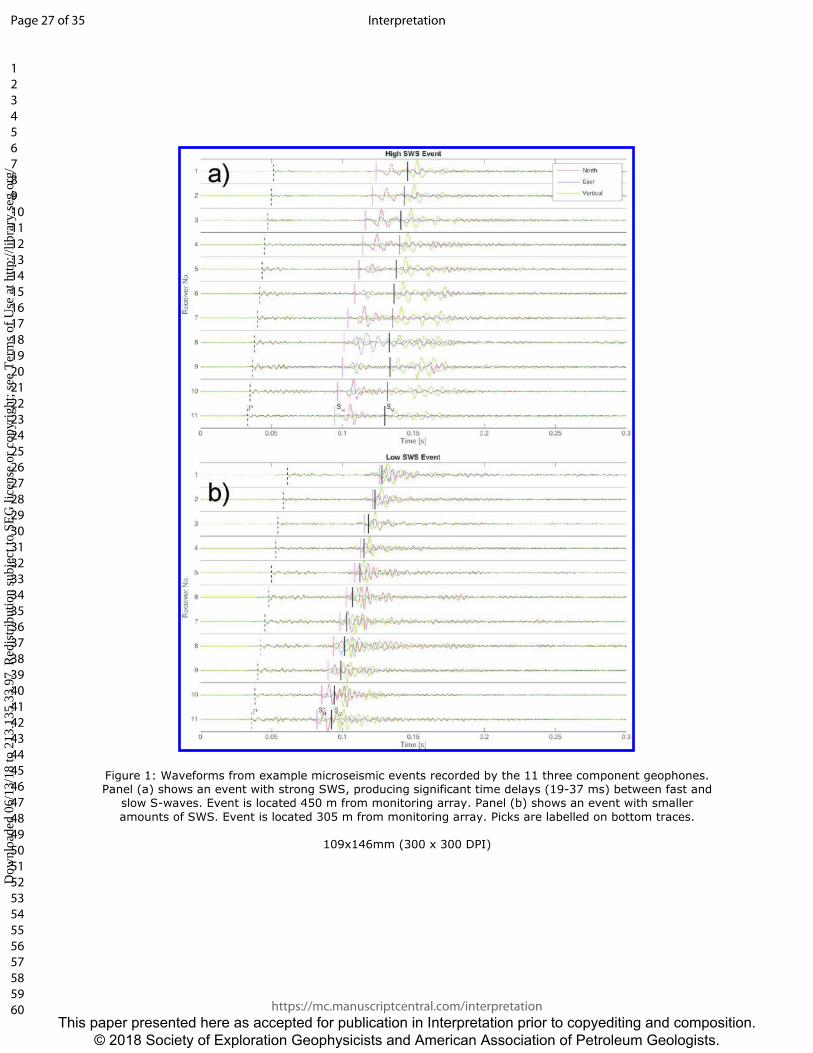
Figure 1: Waveforms from example microseismic events recorded by the 11 three component geophones. Panel (a) shows an event with strong SWS, producing significant time delays (19-37 ms) between fast and

slow S-waves. Event is located 450 m from monitoring array. Panel (b) shows an event with smaller

amounts of SWS. Event is located 305 m from monitoring array. Picks are labelled on bottom traces.

109x146mm (300 x 300 DPI)

Page 27 of 35


Interpretation

123456789101112131415161718192021222324252627282930313233343536373839404142434445464748495051525354555657585960


Dow

nloa

ded

06/1

3/18

to 2

13.1

35.3

3.97

. Red

istr

ibut

ion

subj

ect t

o SE

G li

cens

e or

cop

yrig

ht; s

ee T

erm

s of

Use

at h

ttp://

libra

ry.s

eg.o

rg/












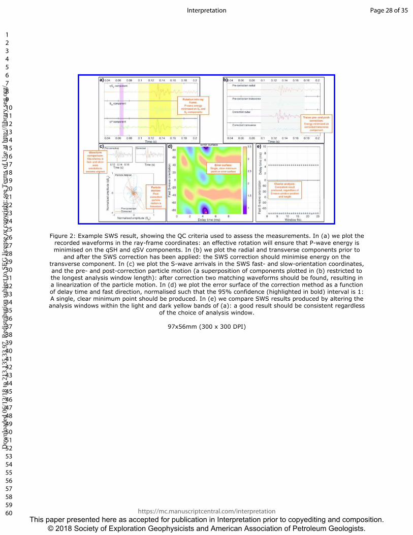
Figure 2: Example SWS result, showing the QC criteria used to assess the measurements. In (a) we plot the recorded waveforms in the ray-frame coordinates: an effective rotation will ensure that P-wave energy is minimised on the qSH and qSV components. In (b) we plot the radial and transverse components prior to

and after the SWS correction has been applied: the SWS correction should minimise energy on the transverse component. In (c) we plot the S-wave arrivals in the SWS fast- and slow-orientation coordinates, and the pre- and post-correction particle motion (a superposition of components plotted in (b) restricted to the longest analysis window length): after correction two matching waveforms should be found, resulting in a linearization of the particle motion. In (d) we plot the error surface of the correction method as a function of delay time and fast direction, normalised such that the 95% confidence (highlighted in bold) interval is 1: A single, clear minimum point should be produced. In (e) we compare SWS results produced by altering the analysis windows within the light and dark yellow bands of (a): a good result should be consistent regardless

of the choice of analysis window.

97x56mm (300 x 300 DPI)

Page 28 of 35


Interpretation

123456789101112131415161718192021222324252627282930313233343536373839404142434445464748495051525354555657585960


Dow

nloa

ded

06/1

3/18

to 2

13.1

35.3

3.97

. Red

istr

ibut

ion

subj

ect t

o SE

G li

cens

e or

cop

yrig

ht; s

ee T

erm

s of

Use

at h

ttp://

libra

ry.s

eg.o

rg/







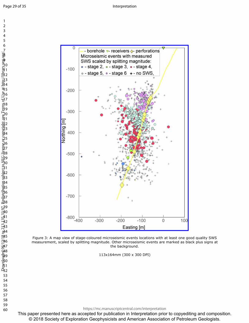
Figure 3: A map view of stage-coloured microseismic events locations with at least one good quality SWS measurement, scaled by splitting magnitude. Other microseismic events are marked as black plus signs at

the background.

113x164mm (300 x 300 DPI)

Page 29 of 35


Interpretation

123456789101112131415161718192021222324252627282930313233343536373839404142434445464748495051525354555657585960


Dow

nloa

ded

06/1

3/18

to 2

13.1

35.3

3.97

. Red

istr

ibut

ion

subj

ect t

o SE

G li

cens

e or

cop

yrig

ht; s

ee T

erm

s of

Use

at h

ttp://

libra

ry.s

eg.o

rg/











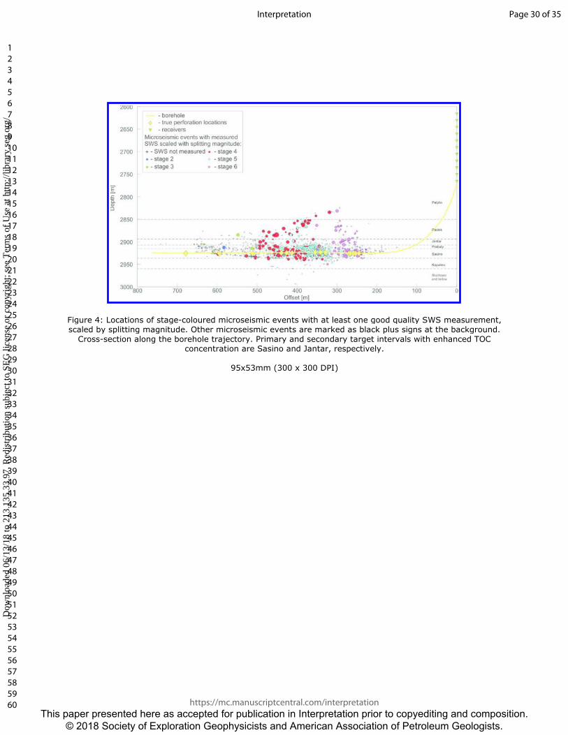
Figure 4: Locations of stage-coloured microseismic events with at least one good quality SWS measurement, scaled by splitting magnitude. Other microseismic events are marked as black plus signs at the background.

Cross-section along the borehole trajectory. Primary and secondary target intervals with enhanced TOC concentration are Sasino and Jantar, respectively.

95x53mm (300 x 300 DPI)

Page 30 of 35


Interpretation

123456789101112131415161718192021222324252627282930313233343536373839404142434445464748495051525354555657585960


Dow

nloa

ded

06/1

3/18

to 2

13.1

35.3

3.97

. Red

istr

ibut

ion

subj

ect t

o SE

G li

cens

e or

cop

yrig

ht; s

ee T

erm

s of

Use

at h

ttp://

libra

ry.s

eg.o

rg/







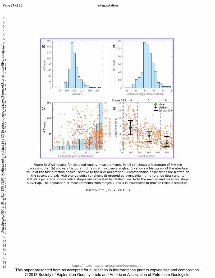
Figure 5: SWS results for the good-quality measurements. Panel (a) shows a histogram of P-wave backazimuths; (b) shows a histogram of ray-path incidence angles; (c) shows a histogram of the absolute value of the fast direction angles (relative to the qSV orientation). Corresponding delay times are plotted on

the secondary axis with orange dots; (d) shows dt ordered by event origin time (orange dots) and its statistics per stage. Consecutive stages are separated by dashed line. Note the median and mean for stage 5 overlap. The population of measurements from stages 2 and 3 is insufficient to provide reliable statistics.

188x168mm (300 x 300 DPI)

Page 31 of 35


Interpretation

123456789101112131415161718192021222324252627282930313233343536373839404142434445464748495051525354555657585960


Dow

nloa

ded

06/1

3/18

to 2

13.1

35.3

3.97

. Red

istr

ibut

ion

subj

ect t

o SE

G li

cens

e or

cop

yrig

ht; s

ee T

erm

s of

Use

at h

ttp://

libra

ry.s

eg.o

rg/










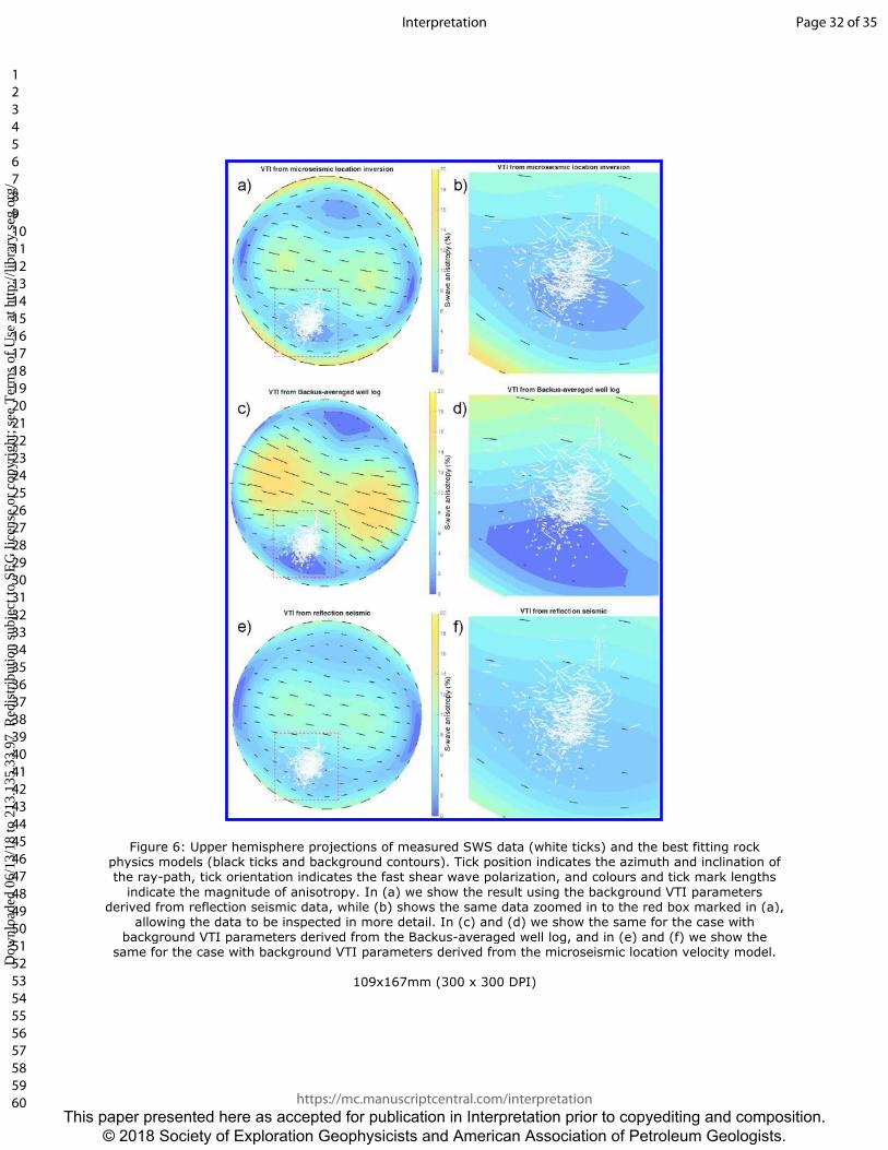
Figure 6: Upper hemisphere projections of measured SWS data (white ticks) and the best fitting rock physics models (black ticks and background contours). Tick position indicates the azimuth and inclination of the ray-path, tick orientation indicates the fast shear wave polarization, and colours and tick mark lengths

indicate the magnitude of anisotropy. In (a) we show the result using the background VTI parameters derived from reflection seismic data, while (b) shows the same data zoomed in to the red box marked in (a),

allowing the data to be inspected in more detail. In (c) and (d) we show the same for the case with background VTI parameters derived from the Backus-averaged well log, and in (e) and (f) we show the

same for the case with background VTI parameters derived from the microseismic location velocity model.

109x167mm (300 x 300 DPI)

Page 32 of 35


Interpretation

123456789101112131415161718192021222324252627282930313233343536373839404142434445464748495051525354555657585960


Dow

nloa

ded

06/1

3/18

to 2

13.1

35.3

3.97

. Red

istr

ibut

ion

subj

ect t

o SE

G li

cens

e or

cop

yrig

ht; s

ee T

erm

s of

Use

at h

ttp://

libra

ry.s

eg.o

rg/










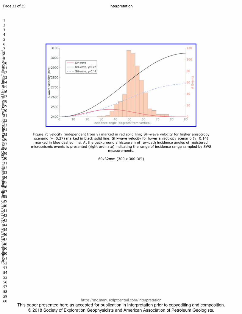
Figure 7: velocity (independent from γ) marked in red solid line; SH-wave velocity for higher anisotropy scenario (γ=0.27) marked in black solid line; SH-wave velocity for lower anisotropy scenario (γ=0.14) marked in blue dashed line. At the background a histogram of ray-path incidence angles of registered

microseismic events is presented (right ordinate) indicating the range of incidence range sampled by SWS measurements.

60x32mm (300 x 300 DPI)

Page 33 of 35


Interpretation

123456789101112131415161718192021222324252627282930313233343536373839404142434445464748495051525354555657585960


Dow

nloa

ded

06/1

3/18

to 2

13.1

35.3

3.97

. Red

istr

ibut

ion

subj

ect t

o SE

G li

cens

e or

cop

yrig

ht; s

ee T

erm

s of

Use

at h

ttp://

libra

ry.s

eg.o

rg/







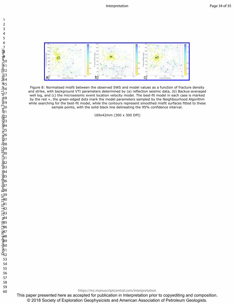
Figure 8: Normalised misfit between the observed SWS and model values as a function of fracture density and strike, with background VTI parameters determined by (a) reflection seismic data, (b) Backus-averaged well log, and (c) the microseismic event location velocity model. The best-fit model in each case is marked by the red +, the green-edged dots mark the model parameters sampled by the Neighbourhood Algorithm while searching for the best-fit model, while the contours represent smoothed misfit surfaces fitted to these

sample points, with the solid black line delineating the 95% confidence interval.

169x42mm (300 x 300 DPI)

Page 34 of 35


Interpretation

123456789101112131415161718192021222324252627282930313233343536373839404142434445464748495051525354555657585960


Dow

nloa

ded

06/1

3/18

to 2

13.1

35.3

3.97

. Red

istr

ibut

ion

subj

ect t

o SE

G li

cens

e or

cop

yrig

ht; s

ee T

erm

s of

Use

at h

ttp://

libra

ry.s

eg.o

rg/




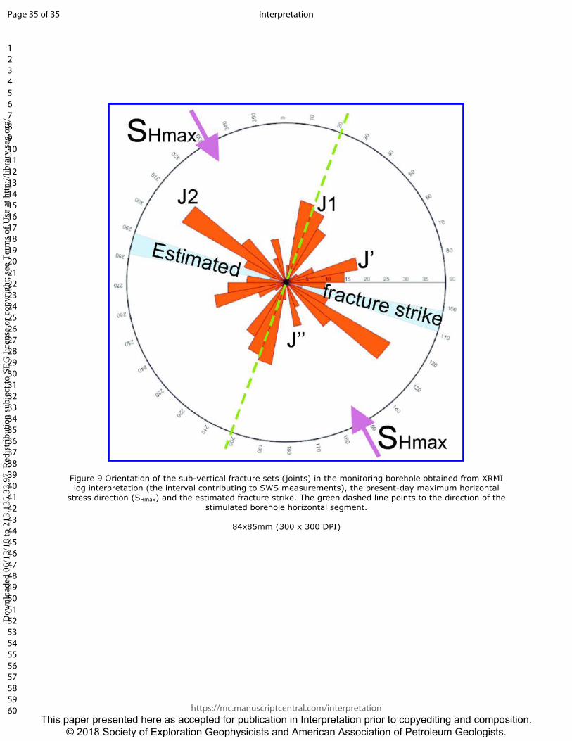
Figure 9 Orientation of the sub-vertical fracture sets (joints) in the monitoring borehole obtained from XRMI log interpretation (the interval contributing to SWS measurements), the present-day maximum horizontal

stress direction (SHmax) and the estimated fracture strike. The green dashed line points to the direction of the

stimulated borehole horizontal segment.

84x85mm (300 x 300 DPI)

Page 35 of 35


Interpretation

123456789101112131415161718192021222324252627282930313233343536373839404142434445464748495051525354555657585960


Dow

nloa

ded

06/1

3/18

to 2

13.1

35.3

3.97

. Red

istr

ibut

ion

subj

ect t

o SE

G li

cens

e or

cop

yrig

ht; s

ee T

erm

s of

Use

at h

ttp://

libra

ry.s

eg.o

rg/











Documents

RESULTS OF THE DOWNHOLE MICROSEISMIC …gljpv/PDFS/Gajek_etal_2018.pdf · The first part of the paper (Gajek et al., 2018) introduces the experiment setting, geology and monitoring