The Astrophysical Journal Supplement Series, 197:26 (13pp), 2011 December doi:10.1088/0067-0049/197/2/26C© 2011. The American Astronomical Society. All rights reserved. Printed in the U.S.A.

RETIRED A STARS AND THEIR COMPANIONS. VII. 18 NEW JOVIAN PLANETS∗

John Asher Johnson1,2, Christian Clanton1,2, Andrew W. Howard3, Brendan P. Bowler4, Gregory W. Henry5,Geoffrey W. Marcy3, Justin R. Crepp1, Michael Endl6, William D. Cochran6, Phillip J. MacQueen6,

Jason T. Wright7,8, and Howard Isaacson41 Department of Astrophysics, California Institute of Technology, MC 249-17, Pasadena, CA 91125, USA; johnjohn@astro.caltech.edu

2 NASA Exoplanet Science Institute (NExScI), CIT Mail Code 100-22, 770 South Wilson Avenue, Pasadena, CA 91125, USA3 Department of Astronomy, University of California, Mail Code 3411, Berkeley, CA 94720, USA4 Institute for Astronomy, University of Hawaii, 2680 Woodlawn Drive, Honolulu, HI 96822, USA

5 Center of Excellence in Information Systems, Tennessee State University, 3500 John A. Merritt Blvd., Box 9501, Nashville, TN 37209, USA6 McDonald Observatory, University of Texas at Austin, TX 78712-0259, USA

7 Department of Astronomy & Astrophysics, The Pennsylvania State University, University Park, PA 16802, USA8 Center for Exoplanets and Habitable Worlds, The Pennsylvania State University, University Park, PA 16802, USA

Received 2011 May 10; accepted 2011 September 26; published 2011 November 29

ABSTRACT

We report the detection of 18 Jovian planets discovered as part of our Doppler survey of subgiant stars at KeckObservatory, with follow-up Doppler and photometric observations made at McDonald and Fairborn Observatories,respectively. The host stars have masses 0.927 � M�/M� � 1.95, radii 2.5 � R�/R� � 8.7, and metallicities−0.46 � [Fe/H] � +0.30. The planets have minimum masses 0.9 MJup � MP sin i �13 MJup and semimajor axesa � 0.76 AU. These detections represent a 50% increase in the number of planets known to orbit stars more massivethan 1.5 M� and provide valuable additional information about the properties of planets around stars more massivethan the Sun.

Key words: binaries: spectroscopic – planetary systems – techniques: photometric – techniques: radial velocities

1. INTRODUCTION

Jupiter-mass planets are not uniformly distributed around allstars in the galaxy. Rather, the rate of planet occurrence is in-timately tied to the physical properties of the stars they or-bit (Johnson et al. 2010a; Howard et al. 2011b; Schlaufman& Laughlin 2011). Radial velocity (RV) surveys have demon-strated that the likelihood that a star harbors a giant planet witha minimum mass MP sin i � 0.5 MJup increases with both stel-lar metallicity and mass9 (Gonzalez 1997a; Santos et al. 2004;Fischer & Valenti 2005; Johnson et al. 2010a; Schlaufman &Laughlin 2010; Brugamyer et al. 2011). This result has bothinformed models of giant planet formation (Ida & Lin 2004;Laughlin et al. 2004; Thommes et al. 2008; Kennedy & Kenyon2008; Mordasini et al. 2009) and pointed the way toward ad-ditional exoplanet discoveries (Laughlin 2000; Marois et al.2008).

The increased abundance of giant planets around massive,metal-rich stars may be a reflection of their more massive,dust-enriched circumstellar disks, which form protoplanetarycores more efficiently (Ida & Lin 2004; Fischer & Valenti 2005;Thommes & Murray 2006; Wyatt et al. 2007). In the searchfor additional planets in the solar neighborhood, metallicity-biased Doppler surveys have greatly increased the numberof close-in, transiting exoplanets around nearby, bright stars,thereby enabling detailed studies of exoplanet atmospheres

∗ Based on observations obtained at the W. M. Keck Observatory and with theHobby-Ebberly Telescope at the McDonald Observatory. Keck is operatedjointly by the University of California and the California Institute ofTechnology. Keck time has been granted by Caltech, the University of Hawaii,NASA, and the University of California.9 Some studies indicate a lack of a planet–metallicity relationship amongplanet-hosting K giants (Pasquini et al. 2007; Sato et al. 2008b). However, aplanet–metallicity correlation is evident among subgiants, which probe anoverlapping range of stellar masses and convective envelope depths (Fischer &Valenti 2005; Johnson et al. 2010a; Ghezzi et al. 2010).

(Fischer et al. 2005; da Silva et al. 2006; Charbonneau et al.2000). Similarly, future high-contrast imaging surveys willlikely benefit from enriching their target lists with intermediate-mass A- and F-type stars (Marois et al. 2008; Crepp & Johnson2011).

Occurrence rate is not the only aspect of exoplanets thatcorrelates with stellar mass. Just when exoplanet researcherswere growing accustomed to short-period and highly eccentricplanets around Sun-like stars, surveys of evolved stars revealedthat the orbital properties of planets are very different at higherstellar masses. Stars more massive than 1.5 M� may have ahigher overall occurrence of Jupiters than do Sun-like stars, butthey exhibit a marked paucity of planets with semimajor axesa � 1 AU (Johnson et al. 2007; Sato et al. 2008a). This is not anobservational bias since close-in, giant planets produce readilydetectable Doppler signals. There is also growing evidence thatplanets around more massive stars tend to have larger minimummasses (Lovis & Mayor 2007; Bowler et al. 2010) and occupyless eccentric orbits compared to planets around Sun-like stars(Johnson 2008).

M-type dwarfs also exhibit a deficit of “hot Jupiters,” al-beit with a lower overall occurrence of giant planets at allperiods (Endl et al. 2003; Johnson et al. 2010a). However, arecent analysis of the transiting planets detected by the space-based Kepler mission shows that the occurrence of close-in,low-mass planets (P < 50 days, MP � 0.1 MJup) increasessteadily with decreasing stellar mass (Howard et al. 2011b).Also counter to the statistics of Jovian planets, low-mass planetsare found quite frequently around low-metallicity stars (Sousaet al. 2008; Valenti et al. 2009). These results strongly sug-gest that stellar mass is a key variable in the formation andsubsequent orbital evolution of planets, and that the forma-tion of gas giants is likely a threshold process that leavesbehind a multitude of “failed cores” with masses of order10 M⊕.

1

The Astrophysical Journal Supplement Series, 197:26 (13pp), 2011 December Johnson et al.

6500 6000 5500 5000 4500Teff [K]

−1.0

−0.5

0.0

0.5

1.0

1.5lo

g(L/

L Sun

)

Figure 1. Distribution of the effective temperatures and luminosities of theKeck sample of subgiants (filled circles) compared with the full CPS Kecktarget sample (gray diamonds).

To study the properties of planets around stars more mas-sive than the Sun, we are conducting a Doppler survey ofintermediate-mass subgiant stars, also known as the “retired”A-type stars (Johnson et al. 2006). Main-sequence stars withmasses greater than ≈1.3 M� (spectral types �F8) are chal-lenging targets for Doppler surveys because they are hot andrapidly rotating (Teff > 6300, Vr sin i � 30 km s−1; Gallandet al. 2005). However, post-main-sequence stars located on thegiant and subgiant branches are cooler and have much slowerrotation rates than their main-sequence cohort. Their spectratherefore exhibit a higher density of narrow absorption linesthat are ideal for precise Doppler-shift measurements.

Our survey has resulted in the detection of 16 planetsaround 14 intermediate-mass (M� � 1.5 M�) stars, includingtwo multiplanet systems, the first Doppler-detected hot Jupiteraround an intermediate-mass star, and 4 additional Jovianplanets around less massive subgiants (Johnson et al. 2006,2007, 2008, 2010b, 2010c, 2011; Bowler et al. 2010; Peek et al.2009). In this contribution we announce the detection of 18 newgiant exoplanets orbiting subgiants spanning a wide range ofstellar physical properties.

2. OBSERVATIONS AND ANALYSIS

2.1. Target Stars

The details of the target selection of our Doppler survey ofevolved stars at Keck Observatory have been described in detailby, e.g., Johnson et al. (2006, 2010c) and Peek et al. (2009).In summary, we have selected subgiants from the Hipparcoscatalog (van Leeuwen 2007) based on B − V colors and absolutemagnitudes MV so as to avoid K-type giants that are observed aspart of other Doppler surveys (e.g., Hatzes et al. 2003; Sato et al.2005; Reffert et al. 2006) and exhibit jitter levels in excess of10 m s−1 (Hekker et al. 2006). We also selected stars in a regionof the temperature–luminosity plane in which stellar model gridsof various masses are well separated and correspond to massesM� > 1.3 M� at solar metallicity according to the Girardi et al.(2002) model grids. However, some of our stars have subsolarmetallicities ([Fe/H] < 0) and correspondingly lower massesdown to ≈1 M�. Our sample of 240 subgiants monitored at KeckObservatory (excluding the Lick Observatory sample described

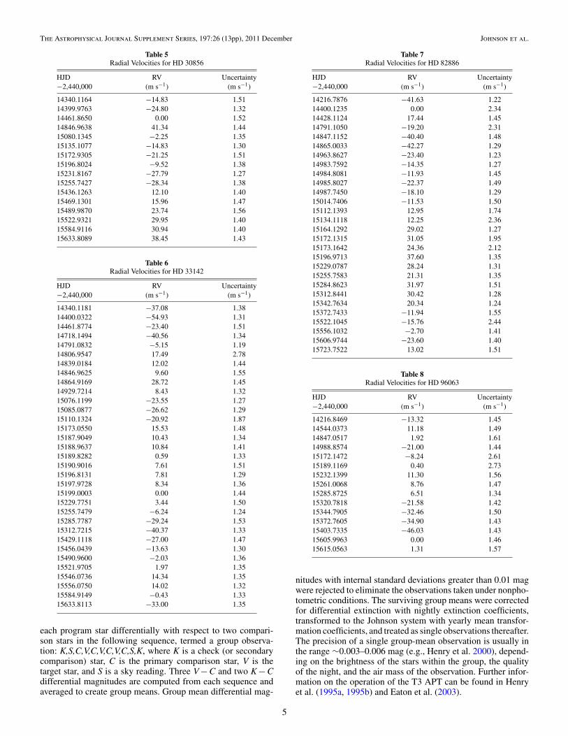
Table 1Radial Velocities for HD 5891

HJD RV Uncertainty−2,440,000 (m s−1) (m s−1)

14339.9257 0.00 1.3214399.8741 14.40 1.4114675.0029 −101.80 1.3314717.9867 59.72 1.4015015.0521 −229.51 1.3215017.1151 −252.49 1.3615048.9850 −47.12 1.4015075.1005 77.03 1.4815076.0885 84.20 1.2315077.0766 88.74 1.3715078.0802 89.43 1.3515079.0828 104.30 1.4015111.8798 −40.60 1.5115135.0589 −113.11 1.3015171.9551 −234.11 1.6315187.7896 −246.19 1.4015196.7607 −148.30 1.3515198.8379 −184.96 1.4115229.7277 13.78 1.2915250.7176 124.93 1.4515255.7218 65.51 1.4015396.1245 −91.80 1.4315404.1162 −66.27 1.2615405.0745 −20.21 1.3915406.0816 −41.20 1.2615407.1010 −31.38 1.2115412.0014 26.94 1.2215414.0290 61.79 1.2015426.1218 103.97 1.2215426.9953 112.44 1.2315427.9420 118.27 1.3715429.0078 115.51 1.0515432.1135 95.23 1.2315433.0935 78.87 1.1815433.9790 61.60 1.1915435.0523 69.27 1.3215438.0958 10.98 1.2715439.0659 64.64 1.3715455.9425 25.71 1.3715467.1200 6.21 1.4515469.1005 −43.24 1.4515470.0312 −67.08 1.2415471.7947 −75.53 1.3615487.0751 −165.74 1.3915489.9608 −183.77 1.5615490.7952 −198.38 1.3715500.8587 −286.77 1.4015522.8948 −274.58 1.3915528.8646 −234.13 1.3415542.8572 −255.45 1.3015544.9247 −261.59 1.5615584.7351 5.02 1.4915613.7133 140.41 2.4015731.1086 −183.76 1.24

by Johnson et al. 2006) is shown in Figure 1 and compared withthe full target sample of the California Planet Survey (CPS).

2.2. Spectra and Doppler-shift Measurements

We obtained spectroscopic observations of our sample ofsubgiants at Keck Observatory using the High ResolutionEchelle Spectrometer (HIRES) with a resolution of R ≈ 55,000

2

The Astrophysical Journal Supplement Series, 197:26 (13pp), 2011 December Johnson et al.

with the B5 decker (0.′′86 width) and red cross-disperser (Vogtet al. 1994). We use the HIRES exposure meter to ensurethat all observations receive uniform flux levels independent ofatmospheric transparency variations and to provide the photon-weighted exposure midpoint, which is used for the barycentriccorrection (BC). Under nominal atmospheric conditions, aV = 8 target requires an exposure time of 90 s and results in asignal-to-noise ratio of 190 at 5800 Å for our sample comprisingmostly early K-type stars.

Normal program observations are made through atemperature-controlled Pyrex cell containing gaseous iodine,which is placed just in front of the entrance slit of the spec-trometer. The dense set of narrow molecular lines imprinted oneach stellar spectrum from 5000 Å to 6200 Å provides a robust,simultaneous wavelength calibration for each observation, aswell as information about the shape of the spectrometer’s in-strumental response (Marcy & Butler 1992). RVs are measuredwith respect to an iodine-free “template” observation that hashad the HIRES instrumental profile removed through decon-volution. Differential Doppler shifts are measured from eachspectrum using the forward-modeling procedure described byButler et al. (1996), with subsequent improvements over theyears by the CPS team (e.g., Howard et al. 2011a). The instru-mental uncertainty of each measurement is estimated based onthe weighted standard deviation of the mean Doppler shift mea-sured from each of ≈700 independent 2 Å spectral regions. In afew instances we made two or more successive observations ofthe same star and averaged the velocities in 2 hr time intervals,thereby reducing the associated measurement uncertainty.

We have also obtained additional spectra for HD 1502 incollaboration with the McDonald Observatory planet searchteam. A total of 54 RV measurements were collected forHD 1502: 32 with the 2.7 m Harlan J. Smith Telescope and itsTull Coude Spectrograph (Tull et al. 1995), and 22 with the HighResolution Spectrograph (HRS; Tull 1998) at the Hobby–EberlyTelescope (Ramsey et al. 1998). On each spectrometer we use asealed and temperature-controlled iodine cell as velocity metricand to allow line-spread function reconstruction. The spectralresolving power for the HRS and Tull spectrograph is set to R =60,000. Precise differential RVs are computed using the AustralI2-data modeling algorithm (Endl et al. 2000).

The RV measurements are listed in Tables 1–18 together withthe Heliocentric Julian Date (HJD) of observation and internalmeasurement uncertainties, excluding the jitter contributiondescribed in Section 2.5.

2.3. Stellar Properties

We use the iodine-free template spectra to estimate atmo-spheric parameters of the target stars with the LTE spectroscopicanalysis package Spectroscopy Made Easy (SME; Valenti &Piskunov 1996), as described by Valenti & Fischer (2005) andFischer & Valenti (2005). Subgiants have lower surface grav-ities than dwarfs, and the damping wings of the Mg i b tripletlines therefore provide weaker constraints on the surface grav-ity, which is in turn degenerate with effective temperature andmetallicity. To constrain log g, we use the iterative scheme ofValenti et al. (2009), which ties the SME-derived value of log gto the gravity inferred from interpolating the stellar luminos-ity, temperature, and metallicity onto the Yonsei–Yale (Y2; Yiet al. 2004) stellar model grids, which also give the stellar ageand mass. The model-based log g is held fixed in a secondSME analysis, and the process is iterated until convergence ismet between the model-based and spectroscopically measured

Table 2Radial Velocities for HD 1502

JD RV Uncertainty Telescope−2,440,000 (m s−1) (m s−1)

14339.927 −40.99 1.81 K14399.840 −37.37 1.92 K14455.835 11.74 1.74 K14675.004 40.95 1.82 K14689.001 43.01 1.82 K14717.944 20.39 1.85 K14722.893 11.99 1.85 K14777.880 −15.02 1.78 K14781.811 −32.99 3.21 M14790.879 −19.32 1.68 K14805.805 −21.62 1.71 K14838.766 −3.59 1.65 K14841.588 −15.98 2.83 M14846.742 −8.77 1.84 K14866.725 −6.17 3.21 K14867.739 −3.89 1.97 K14987.119 65.62 1.74 K15015.051 65.31 1.84 K15016.082 65.49 1.70 K15019.057 68.57 1.96 K15024.909 77.15 2.40 M15027.910 67.88 4.04 M15029.082 80.82 1.89 K15045.070 83.04 1.76 K15053.900 54.41 4.42 M15072.887 40.18 3.92 M15076.088 58.50 1.69 K15081.093 54.00 1.73 K15084.145 46.98 1.87 K15109.892 45.93 2.02 K15133.977 16.31 1.76 K15135.771 12.49 1.54 K15135.819 −30.75 6.17 M15152.711 −13.01 2.33 M15154.769 5.06 1.56 M15169.858 −14.73 1.76 K15171.883 −12.61 1.69 K15172.717 −30.42 4.45 M15172.844 −18.63 1.70 K15177.688 −51.52 5.61 H15181.669 −58.04 5.12 H15182.661 −64.16 3.60 H15183.657 −60.87 2.33 H15185.651 −58.92 3.68 H15187.851 −32.87 1.78 K15188.646 −64.54 3.57 H15188.889 −31.96 1.74 K15189.779 −29.21 1.59 K15190.646 −67.86 2.61 H15190.775 −31.88 1.69 K15193.642 −65.59 3.27 H15196.758 −33.47 1.57 K15197.784 −27.93 1.78 K15198.801 −25.23 1.56 K15202.598 −68.19 1.93 H15209.584 −68.01 3.66 H15221.599 −51.96 3.68 M15222.588 −57.10 2.79 M15223.577 −57.76 3.76 M15226.568 −58.24 3.83 M15227.568 −49.93 2.95 M15229.725 −45.43 1.59 K15231.745 −43.78 1.74 K15250.715 −40.69 1.65 K15256.709 −33.45 1.90 K

3

The Astrophysical Journal Supplement Series, 197:26 (13pp), 2011 December Johnson et al.

Table 2(Continued)

JD RV Uncertainty Telescope−2,440,000 (m s−1) (m s−1)

15377.122 70.88 1.84 K15405.078 82.90 1.85 K15432.807 64.92 2.94 H15435.106 98.34 1.83 K15436.902 78.92 3.02 M15439.994 92.33 2.00 K15455.963 84.41 1.70 K15468.886 59.36 4.34 H15468.888 65.31 4.23 M15487.058 66.84 1.80 K15491.803 24.25 3.66 H15493.853 68.22 5.03 M15497.724 68.26 3.30 M15501.713 42.59 3.69 M15506.780 34.25 2.46 H15511.764 22.16 3.27 H15519.727 21.96 2.76 H15521.871 50.61 1.79 K15527.793 62.95 4.40 M15528.705 65.33 4.01 M15531.704 23.08 5.55 H15543.686 7.39 5.70 H15547.698 24.28 4.99 M15550.578 32.74 5.69 M15554.632 0.00 2.62 H15565.601 −11.84 2.49 H15584.578 0.00 2.54 M15584.732 9.77 1.65 K15613.708 −6.51 1.89 K

Table 3Radial Velocities for HD 18742

HJD RV Uncertainty−2,440,000 (m s−1) (m s−1)

14340.1033 12.26 1.6714399.9466 0.00 1.4514458.8263 −46.91 1.3914690.0728 −43.10 1.6314719.1392 −19.07 1.3614780.0038 −4.84 1.6914790.9573 −4.31 1.6014805.9154 10.55 1.6314838.8094 22.88 1.5514846.8698 35.60 1.6015077.0932 30.15 1.5415109.9772 24.72 1.7915134.9911 15.75 1.6415171.9048 −7.05 1.6515187.8918 −12.06 1.5415229.7703 −19.43 1.3815255.7374 −30.72 1.3415406.1179 −35.69 1.5415437.1255 −18.68 1.4715465.0699 −12.62 1.4815487.0861 −1.40 1.5415521.8936 1.16 1.4715545.8251 10.13 1.5115555.8882 0.54 1.4515584.8925 12.24 1.4415614.7626 10.35 1.69

Table 4Radial Velocities for HD 28678

HJD RV Uncertainty−2,440,000 (m s−1) (m s−1)

14340.0851 −29.22 1.4014399.9815 −59.79 1.4714718.1237 −32.53 1.4614846.9513 −48.79 1.7215080.1261 −7.59 1.3515109.9872 −34.93 1.5415134.0167 −36.54 1.6015171.9170 −50.92 1.5815190.9001 −55.70 1.7115231.9479 −32.09 1.6415260.7954 −32.63 1.5715312.7181 2.99 1.7515411.1309 0.00 1.4315412.1283 9.68 1.3915413.1357 2.29 1.4515414.1303 12.13 1.6315415.1355 0.68 1.3015426.1389 9.15 1.3315427.1383 10.25 1.2515429.1145 7.58 1.3915432.1434 22.34 1.3515433.1437 10.10 1.3615434.1407 8.09 1.1915436.1283 8.63 1.4215437.1348 8.44 1.1815456.0133 1.26 1.2915521.8977 −45.74 1.4315546.0604 −54.63 1.5815584.7710 −51.43 1.4615633.8041 −28.13 1.64

surface gravity, which results in best-fitting estimates of Teff ,log g, [Fe/H], and Vr sin i.

We perform our model-grid interpolations using a Bayesianframework similar to that described by Takeda et al. (2008).We incorporate prior constraints on the stellar mass based onthe stellar initial mass function and the differential evolution-ary timescales of stars in various regions of the theoreticalH-R diagram. These priors tend to decrease the stellar massinferred for a star of a given effective temperature, luminosity,and metallicity compared with a naive interpolation onto thestellar model grids (Lloyd 2011).

We determine the luminosity of each star from the apparentV-band magnitude and parallax from Hipparcos (van Leeuwen2007) and the bolometric correction based on the effective tem-perature relationship given by VandenBerg & Clem (2003).10

Stellar radii are estimated using the Stefan–Boltzmann rela-tionship and the measured L� and Teff . We also measure thechromospheric emission in the Ca ii line cores (Wright et al.2004; Isaacson & Fischer 2010), providing an SHK value on theMt. Wilson system.

The stellar properties of the 18 stars presented herein aresummarized in Table 19.

2.4. Photometric Measurements

We acquired photometric observations of 17 of the 18 plan-etary candidate host stars with the T3 0.4 m automatic photo-metric telescope (APT) at Fairborn Observatory. T3 observed

10 Previous papers in this series (e.g., Johnson et al. 2010c, 2011) incorrectlycited use of the Flower (1996) bolometric corrections.

4

The Astrophysical Journal Supplement Series, 197:26 (13pp), 2011 December Johnson et al.

Table 5Radial Velocities for HD 30856

HJD RV Uncertainty−2,440,000 (m s−1) (m s−1)

14340.1164 −14.83 1.5114399.9763 −24.80 1.3214461.8650 0.00 1.5214846.9638 41.34 1.4415080.1345 −2.25 1.3515135.1077 −14.83 1.3015172.9305 −21.25 1.5115196.8024 −9.52 1.3815231.8167 −27.79 1.2715255.7427 −28.34 1.3815436.1263 12.10 1.4015469.1301 15.96 1.4715489.9870 23.74 1.5615522.9321 29.95 1.4015584.9116 30.94 1.4015633.8089 38.45 1.43

Table 6Radial Velocities for HD 33142

HJD RV Uncertainty−2,440,000 (m s−1) (m s−1)

14340.1181 −37.08 1.3814400.0322 −54.93 1.3114461.8774 −23.40 1.5114718.1494 −40.56 1.3414791.0832 −5.15 1.1914806.9547 17.49 2.7814839.0184 12.02 1.4414846.9625 9.60 1.5514864.9169 28.72 1.4514929.7214 8.43 1.3215076.1199 −23.55 1.2715085.0877 −26.62 1.2915110.1324 −20.92 1.8715173.0550 15.53 1.4815187.9049 10.43 1.3415188.9637 10.84 1.4115189.8282 0.59 1.3315190.9016 7.61 1.5115196.8131 7.81 1.2915197.9728 8.34 1.3615199.0003 0.00 1.4415229.7751 3.44 1.5015255.7479 −6.24 1.2415285.7787 −29.24 1.5315312.7215 −40.37 1.3315429.1118 −27.00 1.4715456.0439 −13.63 1.3015490.9600 −2.03 1.3615521.9705 1.97 1.3515546.0736 14.34 1.3515556.0750 14.02 1.3215584.9149 −0.43 1.3315633.8113 −33.00 1.35

each program star differentially with respect to two compari-son stars in the following sequence, termed a group observa-tion: K,S,C,V,C,V,C,V,C,S,K, where K is a check (or secondarycomparison) star, C is the primary comparison star, V is thetarget star, and S is a sky reading. Three V − C and two K − Cdifferential magnitudes are computed from each sequence andaveraged to create group means. Group mean differential mag-

Table 7Radial Velocities for HD 82886

HJD RV Uncertainty−2,440,000 (m s−1) (m s−1)

14216.7876 −41.63 1.2214400.1235 0.00 2.3414428.1124 17.44 1.4514791.1050 −19.20 2.3114847.1152 −40.40 1.4814865.0033 −42.27 1.2914963.8627 −23.40 1.2314983.7592 −14.35 1.2714984.8081 −11.93 1.4514985.8027 −22.37 1.4914987.7450 −18.10 1.2915014.7406 −11.53 1.5015112.1393 12.95 1.7415134.1118 12.25 2.3615164.1292 29.02 1.2715172.1315 31.05 1.9515173.1642 24.36 2.1215196.9713 37.60 1.3515229.0787 28.24 1.3115255.7583 21.31 1.3515284.8623 31.97 1.5115312.8441 30.42 1.2815342.7634 20.34 1.2415372.7433 −11.94 1.5515522.1045 −15.76 2.4415556.1032 −2.70 1.4115606.9744 −23.60 1.4015723.7522 13.02 1.51

Table 8Radial Velocities for HD 96063

HJD RV Uncertainty−2,440,000 (m s−1) (m s−1)

14216.8469 −13.32 1.4514544.0373 11.18 1.4914847.0517 1.92 1.6114988.8574 −21.00 1.4415172.1472 −8.24 2.6115189.1169 0.40 2.7315232.1399 11.30 1.5615261.0068 8.76 1.4715285.8725 6.51 1.3415320.7818 −21.58 1.4215344.7905 −32.46 1.5015372.7605 −34.90 1.4315403.7335 −46.03 1.4315605.9963 0.00 1.4615615.0563 1.31 1.57

nitudes with internal standard deviations greater than 0.01 magwere rejected to eliminate the observations taken under nonpho-tometric conditions. The surviving group means were correctedfor differential extinction with nightly extinction coefficients,transformed to the Johnson system with yearly mean transfor-mation coefficients, and treated as single observations thereafter.The precision of a single group-mean observation is usually inthe range ∼0.003–0.006 mag (e.g., Henry et al. 2000), depend-ing on the brightness of the stars within the group, the qualityof the night, and the air mass of the observation. Further infor-mation on the operation of the T3 APT can be found in Henryet al. (1995a, 1995b) and Eaton et al. (2003).

5

The Astrophysical Journal Supplement Series, 197:26 (13pp), 2011 December Johnson et al.

Table 9Radial Velocities for HD 98219

HJD RV Uncertainty−2,440,000 (m s−1) (m s−1)

14216.8449 57.96 1.1314544.0427 19.96 1.5214640.7494 51.97 2.0914847.0563 −32.03 1.4114983.7787 19.55 1.2915171.1635 10.20 1.3315189.1341 4.18 2.4815229.0611 −16.08 1.3015252.0420 −23.02 1.2615255.8857 −23.18 1.2415285.8704 −19.25 1.3015313.8334 −25.03 1.2915342.7941 −12.41 1.2615376.7390 0.00 1.2515585.1462 33.03 1.3315606.0328 16.94 1.2815700.7708 −33.64 1.23

Table 10Radial Velocities for HD 99706

HJD RV Uncertainty−2,440,000 (m s−1) (m s−1)

14428.1613 38.42 1.2714429.0887 35.89 1.2914464.0610 26.33 1.4914847.0764 4.66 1.3914988.8390 0.00 1.2915174.1629 33.84 1.2315229.0719 34.84 1.2215255.9592 31.65 1.1815256.9781 28.77 1.2015284.9159 23.61 1.2815313.9492 16.02 1.1915343.8495 12.69 1.2115378.7470 −2.49 1.3015404.7331 −0.41 1.2315543.1727 −8.84 1.1915585.1087 −12.15 1.1515605.9817 −25.72 1.3315615.0400 −20.42 1.3515633.9015 −20.59 1.2715663.9636 −12.73 1.2015667.9704 −12.98 1.1815700.8151 −19.50 1.2015734.7675 −15.18 1.1115770.7434 −13.48 1.37

Our photometric observations are useful for eliminatingpotential false positives from our sample of new planets. Forexample, Queloz et al. (2001) and Paulson et al. (2004) havedemonstrated how rotational modulation in the visibility ofstarspots on active stars can result in periodic RV variationsand, therefore, the potential for erroneous planetary detections.Photometric results for the 17 stars in the present sample aregiven in Table 20. Columns 7–10 give the standard deviationsof the V − C and K − C differential magnitudes in the V andB passbands with 3σ outliers removed. All of the standarddeviations are small and consistent with the measurementprecision of the telescope. Periodogram analysis of each dataset found no significant periodicity between 1 and 100 days.

Table 11Radial Velocities for HD 102329

HJD RV Uncertainty−2,440,000 (m s−1) (m s−1)

14216.8413 −60.44 1.2014544.0391 19.90 1.2314847.0691 28.39 1.3214988.8623 −68.46 1.2615015.8197 −84.27 1.1515044.7343 −107.42 1.1915172.1434 −78.90 2.5115189.1143 −72.33 2.3115229.0638 −51.88 1.2215255.8881 −28.90 1.1515289.9324 10.79 1.1815313.7792 10.12 1.1415342.7984 21.54 1.1015373.7400 38.91 1.2215402.7556 31.52 1.3015606.0374 29.79 1.1515615.0521 21.05 1.2915633.8900 0.00 1.0915667.9885 −11.60 1.1815700.7689 −8.16 1.26

Table 12Radial Velocities for HD 106270

HJD RV Uncertainty−2,440,000 (m s−1) (m s−1)

14216.8355 23.22 1.3814455.1699 102.95 1.6014635.7675 171.13 1.5914927.9701 164.37 1.7515015.8167 121.36 1.3915044.7394 81.25 1.6715173.1299 34.41 2.6015189.1367 28.32 2.6315261.0094 0.00 1.5915289.9478 8.14 1.5615313.8402 −8.69 1.5915342.8011 −21.05 1.5615372.7641 −39.39 1.5215403.7637 −34.73 1.6215585.1385 −38.04 2.6615606.0379 −70.38 1.6115607.0551 −68.71 1.5915633.8911 −58.47 1.5715663.8909 −64.68 1.6515700.7732 −70.54 1.41

We conclude that all 17 planetary candidate stars in Table 20,as well as all of their comparison and check stars, are constantto the limit of our photometric precision. The lack of evidencefor photometric variability provides support for the planetaryinterpretation of the RV variations.

Although we do not have photometric measurements ofHD 142245, we note from Table 19 that HD 142245 has one ofthe lowest values for SHK in the sample. Therefore, like the restof the sample, HD 142245 should be photometrically stable.

2.5. Orbit Analysis

As in Johnson et al. (2010c), we perform a thorough searchof the RV time series of each star for the best-fitting Keplerianorbital model using the partially linearized, least-squares fitting

6

The Astrophysical Journal Supplement Series, 197:26 (13pp), 2011 December Johnson et al.

Table 13Radial Velocities for HD 108863

HJD RV Uncertainty−2,440,000 (m s−1) (m s−1)

14216.8115 −51.43 1.1214544.0479 0.00 1.4114635.8266 −46.44 1.0014934.8653 31.90 1.4714963.9885 24.25 1.3114983.8915 13.21 1.2115014.7747 −13.40 1.1915016.8627 −17.30 1.2115043.7450 −30.01 1.5115172.1413 −28.18 1.5215189.1458 −21.38 2.9515255.8905 20.25 1.2115284.8821 41.28 1.4215311.8035 39.04 1.5015342.8757 40.04 1.2415376.7831 32.40 1.1415402.7515 13.40 1.2615522.1564 −42.12 2.7815546.1659 −56.68 1.2915585.0903 −46.64 1.2515605.9932 −21.93 1.3315634.0020 −16.91 1.3015663.9420 4.31 1.3015704.8126 11.83 1.25

Table 14Radial Velocities for HD 116029

HJD RV Uncertainty−2,440,000 (m s−1) (m s−1)

14216.8196 −26.73 1.0914216.9475 −24.06 0.9614345.7641 20.59 1.3314635.8322 −9.41 1.0214954.9950 −6.09 1.2714983.9004 −2.38 1.1815043.7491 29.89 1.3115197.1540 44.61 1.2115232.0265 21.80 1.2915261.0304 28.04 1.2115285.1540 20.95 1.2815313.7736 4.96 1.0515342.8932 −0.75 1.1815379.8156 −15.82 1.0815404.7751 −25.43 1.1015585.1319 −0.25 1.1315605.9881 −5.74 1.1915615.0443 0.66 1.3115633.9001 0.00 1.1515667.9740 14.75 1.1815703.7976 16.39 1.09

procedure described in Wright & Howard (2009) and imple-mented in the IDL package RVLIN.11 The free parameters in ourmodel are the velocity semiamplitude K, period P, argument ofperiastron ω, time of periastron passage Tp, and the systemicvelocity offset γ . When fitting RVs from separate observato-ries, we include additional offsets γi for the different data sets.As described in Section 2.6, we also explore the existence of aconstant acceleration γ in each RV time series.

11 http://exoplanets.org/code/

Table 15Radial Velocities for HD 131496

HJD RV Uncertainty−2,440,000 (m s−1) (m s−1)

14257.7864 48.99 1.0814339.7383 22.17 1.1514633.8320 −11.45 1.0614674.7923 −24.32 1.1914964.0661 24.79 1.0815041.8436 56.78 1.3015042.8783 41.12 1.2815081.7136 49.43 1.1915197.1629 32.75 1.2915231.1524 29.08 1.2915257.0130 14.66 1.3515284.8831 2.07 1.3515314.8533 0.83 1.4615343.7940 5.12 1.2215379.8222 −13.69 1.2215404.7802 −19.04 1.1815455.7491 −27.49 1.2415546.1613 −14.23 1.3015559.1657 −2.79 1.4215606.0439 −26.97 1.1915607.0571 −22.07 1.2115608.0288 −8.97 1.1315614.0246 −9.23 1.1615615.0451 −10.64 1.4115634.0616 −6.55 1.2415634.9982 −18.47 1.3515635.9791 −2.28 1.0115636.9679 −16.86 1.3415663.9449 0.07 1.3415670.9602 −9.97 0.6315671.8330 2.24 1.0315672.8200 0.63 1.1915673.8340 2.12 1.2515697.8643 7.12 1.4315698.8647 4.48 1.2915699.8226 −0.13 1.2115700.8064 5.34 1.2715703.7722 −2.25 1.1715704.7987 4.89 1.1715705.8142 0.84 1.0415722.9642 0.00 1.30

In addition to the parameters describing the orbit, we alsoinclude an additional error contribution to our RV measurementsdue to stellar “jitter,” which we denote by s. The jitter accountsfor any unmodeled noise sources intrinsic to the star such asrotational modulation of surface inhomogeneities and pulsation(Saar et al. 1998; Wright 2005; Makarov et al. 2009; Lagrangeet al. 2010) and is added in quadrature to the internal uncertaintyof each RV measurement.

Properly estimating the jitter contribution to the uncertainty ofeach measurement is key to accurately estimating the confidenceintervals for each fitted parameter. Ignoring jitter will lead tounderestimated parameter uncertainties, rendering them lessuseful in future statistical investigations of exoplanet properties.Similarly, the equally common practice relying on a single valueof the jitter based on stars with properties similar to the target ofinterest ignores variability in the jitter observed from star to starand can potentially overestimate the parameter uncertainties.For these reasons we take the approach of allowing the jitter

7

The Astrophysical Journal Supplement Series, 197:26 (13pp), 2011 December Johnson et al.

Table 16Radial Velocities for HD 142245

HJD RV Uncertainty−2,440,000 (m s−1) (m s−1)

14257.7609 −1.70 1.0014339.7424 −20.45 1.1414399.6984 −11.61 1.1314635.8973 −31.07 1.2014674.7988 −15.51 1.1714986.8193 20.63 1.1315015.9357 14.23 1.0615231.1494 23.37 1.3215257.0130 21.99 1.0915286.0067 22.97 1.1715319.9358 10.28 1.1115351.8205 15.55 0.9815379.7723 15.15 1.0515464.7090 0.00 1.0315486.6972 7.93 1.1815608.0546 −11.90 1.2115634.0617 −15.12 1.1915700.8053 −11.29 1.2315722.7901 −22.27 1.28

Table 17Radial Velocities for HD 152581

HJD RV Uncertainty−2,440,000 (m s−1) (m s−1)

14257.7825 0.00 1.3614339.7455 −16.51 1.4914399.7115 −17.18 1.6714674.8143 61.42 1.4014963.8491 −7.59 1.5814983.7976 −17.46 1.6715043.8501 −10.75 1.5215111.7059 −13.43 1.5015320.0287 45.27 1.4815342.8146 51.83 1.4215373.7703 56.30 1.6315405.8067 49.53 1.5015435.7358 54.46 1.5015464.7138 46.73 1.5815486.7241 34.80 1.5515606.1541 −4.01 1.4115607.1341 4.78 1.4915608.1201 15.57 1.4615613.1531 8.45 1.3915614.1706 −3.19 1.4415636.0731 −2.34 1.2715668.0300 −14.89 1.5115706.8514 −15.33 1.3115735.8586 −16.72 1.61

term to vary in our orbit analyses, as described by, e.g., Ford &Gregory (2007).

We estimate parameter uncertainties using a Markov ChainMonte Carlo (MCMC) algorithm (see, e.g., Ford 2005; Winnet al. 2007). MCMC is a Bayesian inference technique that usesthe data together with prior knowledge to explore the shape ofthe posterior probability density function (pdf) for each param-eter of an input model. MCMC with the Metropolis–Hastingsalgorithm in particular provides an efficient means of exploringhigh-dimensional parameter space and mapping out the poste-rior pdf for each model parameter.

Table 18Radial Velocities for HD 158038

HJD RV Uncertainty−2,440,000 (m s−1) (m s−1)

14258.0333 −32.20 1.1114287.8726 −28.05 2.3414345.8015 −4.80 1.2214399.7044 14.16 1.2514674.8733 −1.99 1.1714955.9772 42.82 1.3315014.8461 41.88 1.3415028.9808 35.15 1.3015111.7333 7.37 1.2515135.7129 −0.97 1.1215286.0608 −10.73 1.3115313.9043 −21.31 1.1515342.9667 −17.68 1.1715378.7929 −4.90 1.2215399.9588 −1.89 1.2415405.7727 −9.12 1.1215431.7305 6.04 1.2115469.7065 28.63 1.2415585.1729 22.56 1.1615606.1764 15.81 1.0815636.0867 5.26 1.1215668.0043 −11.54 1.1315704.8546 −9.72 1.1615722.8918 −24.06 1.23

At each chain link in our MCMC analysis, one parameter isselected at random and is altered by drawing a random variatefrom a transition probability distribution. If the resulting valueof the likelihood L for the trial orbit is greater than the previousvalue, then the trial orbital parameters are accepted and addedto the chain. If not, then the probability of adopting the newvalue is set by the ratio of the probabilities from the previousand current trial steps. If the current trial is rejected, then theparameters from the previous step are adopted. The size of thetransition function determines the efficiency of convergence. If itis too narrow, then the full exploration of parameter space is slowand the chain is susceptible to local minima; if it is too broad,then the chain exhibits large jumps and the acceptance ratesare low.

Rather than minimizing χ2ν , we maximize the logarithm of

the likelihood of the data, given by

lnL = −Nobs∑i=1

ln√

2π (σi + s)2 − 1

2

Nobs∑i=1

[vi − vm(ti)

σi + s

]2

, (1)

where vi and σi are the ith velocity measurement and itsassociated measurement error, vm(ti) is the Keplerian modelat time ti, s is the jitter, and the sum is performed over all Nobsmeasurements. If s = 0, then the first term on the right side—thenormalization of the probability—is a constant, and the secondterm becomes 1

2χ2. Thus, maximizing lnL is equivalent tominimizing χ2. Larger jitter values more easily accommodatelarge deviations of the observed RV from the model prediction,but only under the penalty of a decreasing (more negative)normalization term, which makes the overall likelihood smaller.

We impose uninformative priors for most of the free parame-ters (either uniform or modified Jeffreys; e.g., Gregory & Fischer2010). The notable exception is jitter, for which we use aGaussian prior with a mean of 5.1 m s−1 and a standard deviationof 1.5 m s−1 based on the distribution of jitter values for a

8

The Astrophysical Journal Supplement Series, 197:26 (13pp), 2011 December Johnson et al.

Table 19Stellar Parameters

Star V B − V Distance MV [Fe/H] Teff Vr sin i log g M∗ R∗ L∗ Age SHK

(pc) (K) (km s−1) (cgs) (M�) (R�) (R�) (Gyr)(1) (2) (3) (4) (5) (6) (7) (8) (9) (10) (11) (12) (13) (14)

HD 1502 8.52 0.92 159(19) 2.5(0.3) 0.09(0.03) 5049(44) 2.70(0.5) 3.4(0.06) 1.61(0.11) 4.5(0.1) 11.6(0.5) 2.4(0.5) 0.146HD 5891 8.25 0.99 251(76) 1.3(0.7) -0.02(0.03) 4907(44) 4.95(0.5) 2.9(0.06) 1.91(0.13) 8.7(0.2) 39.4(0.8) 1.5(0.8) 0.108HD 18742 7.97 0.94 135(14) 2.3(0.2) -0.04(0.03) 5048(44) 2.98(0.5) 3.3(0.06) 1.60(0.11) 4.9(0.1) 13.9(0.5) 2.3(0.5) 0.133HD 28678 8.54 1.01 227(48) 1.8(0.5) -0.11(0.03) 5076(44) 2.97(0.5) 3.3(0.06) 1.74(0.12) 6.2(0.1) 22.9(0.6) 1.8(0.7) 0.130HD 30856 8.07 0.961 118.1(9.9) 2.7(0.2) -0.06(0.03) 4982(44) 2.85(0.5) 3.4(0.06) 1.35(0.094) 4.2(0.1) 9.9(0.5) 3.8(1) 0.130HD 33142 8.13 0.95 126(11) 2.6(0.1) +0.05(0.03) 5052(44) 2.97(0.5) 3.5(0.06) 1.48(0.10) 4.2(0.1) 10.5(0.5) 3.0(0.4) 0.140HD 82886 7.78 0.864 125(12) 2.3(0.1) -0.31(0.03) 5112(44) 0.43(0.5) 3.4(0.06) 1.06(0.074) 4.8(0.1) 13.9(0.5) 7(2) 0.135HD 96063 8.37 0.86 158(20) 2.4(0.3) -0.30(0.03) 5148(44) 0.87(0.5) 3.6(0.06) 1.02(0.072) 4.5(0.1) 12.7(0.5) 9(3) 0.146HD 98219 8.21 0.96 134(12) 2.6(0.2) -0.02(0.03) 4992(44) 0.30(0.5) 3.5(0.06) 1.30(0.091) 4.5(0.1) 11.2(0.5) 4(1) 0.136HD 99706 7.81 1.0 129(11) 2.3(0.2) +0.14(0.03) 4932(44) 0.89(0.5) 3.2(0.06) 1.72(0.12) 5.4(0.1) 15.4(0.5) 2.1(0.4) 0.132HD 102329 8.04 1.04 158(21) 2.1(0.3) +0.30(0.03) 4830(44) 2.60(0.5) 3.0(0.06) 1.95(0.14) 6.3(0.1) 19.6(0.5) 1.6(0.4) 0.129HD 106270 7.73 0.74 84.9(5.7) 3.1(0.2) +0.08(0.03) 5638(44) 3.13(0.5) 3.9(0.06) 1.32(0.092) 2.5(0.1) 5.7(0.5) 4.3(0.6) 0.186HD 108863 7.89 0.99 139(15) 2.2(0.2) +0.20(0.03) 4956(44) 1.06(0.5) 3.2(0.06) 1.85(0.13) 5.6(0.1) 16.8(0.5) 1.8(0.4) 0.127HD 116029 8.04 1.009 123.2(9.9) 2.6(0.2) +0.18(0.03) 4951(44) 0.46(0.5) 3.4(0.06) 1.58(0.11) 4.6(0.1) 11.3(0.5) 2.7(0.5) 0.133HD 131496 7.96 1.04 110.0(9.4) 2.8(0.2) +0.25(0.03) 4927(44) 0.48(0.5) 3.3(0.06) 1.61(0.11) 4.3(0.1) 9.8(0.5) 2.7(0.5) 0.121HD 142245 7.63 1.04 109.5(7.4) 2.4(0.1) +0.23(0.03) 4878(44) 2.66(0.5) 3.3(0.06) 1.69(0.12) 5.2(0.1) 13.5(0.5) 2.3(0.3) 0.122HD 152581 8.54 0.90 186(33) 2.2(0.4) -0.46(0.03) 5155(44) 0.50(0.5) 3.4(0.06) 0.927(0.065) 4.8(0.1) 14.9(0.6) 12(3) 0.146HD 158038 7.64 1.04 103.6(7.9) 2.6(0.1) +0.28(0.03) 4897(44) 1.66(0.5) 3.2(0.06) 1.65(0.12) 4.8(0.1) 11.9(0.5) 2.5(0.3) 0.119

similar sample of intermediate-mass subgiants from Johnsonet al. (2010c).

We use the best-fitting parameter values from RVLIN as ini-tial guesses for our MCMC analysis. We choose normal tran-sition probability functions with constant (rather than adaptive)widths. The standard deviations are iteratively chosen from aseries of smaller chains so that the acceptance rates for eachparameter are between 20% and 30%; each main chain is thenrun for 107 steps. The initial 10% of the chains are excludedfrom the final estimation of parameter uncertainties to ensureuniform convergence. We select the 15.9 and 84.1 percentilelevels in the posterior distributions as the “1σ” confidence lim-its. In most cases the posterior probability distributions wereapproximately Gaussian.

2.6. Testing RV Trends

To determine whether there is evidence for a linear velocitytrend, we use two separate methods: the Bayesian InformationCriterion (BIC; Schwarz 1978; Liddle 2004) and inspectionof the MCMC posterior pdfs, as described by Bowler et al.(2010). The BIC rewards better-fitting models but penalizesoverly complex models, and is given by

BIC ≡ −2 lnLmax + k ln N, (2)

where Lmax is the maximum likelihood for a particular modelwith k free parameters and N data points. The relationshipbetween Lmax and χ2

min is only valid under the assumption thatthe RVs are normally distributed, which is approximately validfor our analyses. A difference of �2 between BIC values withand without a trend indicates that there is sufficient evidence fora more complex model (Kuha 2004).

We also use the MCMC-derived pdf for the velocity trendparameter to estimate the probability that a trend is actuallypresent in the data. We only adopt the model with the trend ifthe 99.7 percentile of the pdf lies above or below 0 m s−1 yr−1.The BIC and MCMC methods yield consistent results for theplanet candidates presented in Section 3, and in many cases theRV trend is evident by visual inspection of Figures 2 and 3.

3. RESULTS

We have detected eighteen new Jovian planets orbitingevolved, subgiant stars. The RV time series of each host staris plotted in Figures 2 and 3, where the error bars show thequadrature sum of the internal errors and the jitter estimate asdescribed in Section 2.5. The RV measurements for each starare listed in Tables 1–18, together with the Julian Date of ob-servation and the internal measurement uncertainties (withoutjitter). The best-fitting orbital parameters and physical charac-teristics of the planets are summarized in Table 21, along withtheir uncertainties. When appropriate we list notes for some ofthe individual planetary systems.

HD 5891, HD 18742, HD 82886, HD 116029, HD 99706,and HD 158038. The orbit models for these stars include lineartrends, which we interpret as additional orbital companions withperiods longer than the time baseline of the observations.

HD 96063. The period of this system is very close to 1 yr,raising the spectra such that it may be an annual systematic errorrather than an actual planet. However, any such annual signalwould most likely be related to an error in the BC and, if present,would cause the RVs to correlate with the BC. We checked andfound no such correlation between RV and BC. Further, wehave never seen an annual signal with an amplitude of thismagnitude in any of the several thousand targets monitored atKeck Observatory.

HD 106270. The reported orbit for this companion is long pe-riod and we only have limited phase coverage in measurements.In addition to the best-fitting, shorter-period orbit, in Figure 4we provide a χ2 contour plot showing the correlation betweenP and MP sin i, similar to Figure 3 of Wright et al. (2009). Thegray scale shows the minimum value of χ2 for single-planetKeplerian fits at fixed values of period and minimum planetmass. The solid contours denote locations at which χ2 increasesby factors of {1, 4, 9} from inside out. The dashed contours showconstant eccentricities e = {0.2, 0.6, 0.9} from left to right.For periods P < 100 yr the ≈99% upper limit on MP sin i is20 MJup, with an extremely high eccentricity near e = 0.9. Foreccentricities e < 0.6, MP sin i <13 MJup at ≈68% confidenceand MP sin i <15 MJup at ≈99% confidence. Given the rarity of

9

The Astrophysical Journal Supplement Series, 197:26 (13pp), 2011 December Johnson et al.

2007 2008 2009 2010 2011−100

−50

0

50

HD 1502

2007 2008 2009 2010 2011Year

−200

−100

0

100

200

300 HD 5891

2007 2008 2009 2010 2011Year

−60

−40

−20

0

20

40

60 HD 18742

2007 2008 2009 2010 2011Year

−40

−20

0

20

40HD 28678

2007 2008 2009 2010 2011Year

−60

−40

−20

0

20

40 HD 30856

2007 2008 2009 2010 2011Year

−40

−20

0

20

40

60 HD 33142

2007 2008 2009 2010 2011−60

−40

−20

0

20

40

60HD 82886

2007 2008 2009 2010 2011

−20

0

20

40HD 96063

2007 2008 2009 2010 2011

−40

−20

0

20

40

60

80HD 98219R

adia

l Vel

ocity

[m s

−1 ]

Year

Figure 2. Relative RVs of nine stars measured at Keck Observatory. The error bars are the quadrature sum of the internal measurement uncertainties and jitter estimates.The dashed line shows the best-fitting orbit solution of a single Keplerian orbit, with a linear trend where appropriate.

2007 2008 2009 2010 2011Year

−40

−20

0

20

40

60

80 HD 99706

2007 2008 2009 2010 2011Year−150

−100

−50

0

50

100HD 102329

2007 2008 2009 2010 2011Year−100

0

100

200

HD 106270

2007 2008 2009 2010 2011Year

−60

−40

−20

0

20

40

60HD 108863

2007 2008 2009 2010 2011

−40

−20

0

20

40

60 HD 116029

2007 2008 2009 2010 2011

−40

−20

0

20

40

60

80HD 131496

2007 2008 2009 2010 2011

−40

−20

0

20

HD 142245

2007 2008 2009 2010 2011

−40

−20

0

20

40

60 HD 152581

2007 2008 2009 2010 2011

−200−100

0100 HD 158038

2007 2008 2009 2010 2011−40−20

0204060

Rad

ial V

eloc

ity [m

s−

1 ]

Year

Figure 3. Relative RVs of nine stars measured at Keck Observatory. The error bars are the quadrature sum of the internal measurement uncertainties and jitter estimates.The dashed line shows the best-fitting orbit solution of a single Keplerian orbit. The split, lower-right panel shows the orbit of HD 158038 with a linear trend (top) andwith the trend removed (bottom).

10

The Astrophysical Journal Supplement Series, 197:26 (13pp), 2011 December Johnson et al.

Table 20Summary of Photometric Observations from Fairborn Observatory

Program Comparison Check Date Range Duration σ (V − C)V σ (V − C)B σ (K − C)V σ (K − C)BStar Star Star (HJD − 2,400,000) (days) Nobs (mag) (mag) (mag) (mag) Variability(1) (2) (3) (4) (5) (6) (7) (8) (9) (10) (11)

HD 1502 HD 3087 HD 3434 54756–55578 822 236 0.0044 0.0042 0.0052 0.0037 ConstantHD 5891 HD 5119 HD 4568 55167–55588 421 82 0.0058 0.0045 0.0046 0.0044 ConstantHD 18742 HD 18166 HD 20321 55167–55599 432 216 0.0066 0.0051 0.0076 0.0058 ConstantHD 28678 HD 28736 HD 28978 55241–55637 396 118 0.0037 0.0035 0.0052 0.0035 ConstantHD 30856 HD 30051 HD 30238 55241–55617 376 210 0.0069 0.0057 0.0080 0.0068 ConstantHD 33142 HD 33093 HD 34045 55104–55639 535 341 0.0054 0.0046 0.0063 0.0070 ConstantHD 82886 HD 81440 HD 81039 55128–55673 545 252 0.0045 0.0036 0.0059 0.0060 ConstantHD 96063 HD 94729 HD 96855 55554–55673 119 92 0.0061 0.0037 0.0052 0.0034 ConstantHD 98219 HD 96483 HD 98346 55554–55673 119 162 0.0073 0.0050 0.0085 0.0077 ConstantHD 99706 HD 99984 HD 101620 55554–55673 119 167 0.0030 0.0032 0.0033 0.0030 ConstantHD 102329 HD 101730 HD 100563 55241–55673 432 169 0.0053 0.0040 0.0046 0.0048 ConstantHD 106270 HD 105343 HD 105205 55241–55671 430 161 0.0059 0.0055 0.0061 0.0059 ConstantHD 108863 HD 109083 HD 107168 55241–55674 433 191 0.0046 0.0037 0.0047 0.0035 ConstantHD 116029 HD 116316 HD 118244 55242–55673 431 181 0.0044 0.0034 0.0048 0.0041 ConstantHD 131496 HD 130556 HD 129537 55242–55673 431 159 0.0044 0.0044 0.0050 0.0046 ConstantHD 152581 HD 153796 HD 153376 55577–55674 97 111 0.0050 0.0053 0.0066 0.0052 ConstantHD 158038 HD 157565 HD 157466 55122–55674 552 155 0.0044 0.0037 0.0044 0.0037 Constant

Table 21Orbital Parameters

Planet Period Tpa Eccentricityb K ω MP sin i a Linear Trend rms Jitter Nobs

(d) (HJD−2,440,000) (m s−1) (deg) (MJup) (AU) (m s−1 yr−1) (m s−1) (m s−1)(1) (2) (3) (4) (5) (6) (7) (8) (9) (10) (11) (12)

HD 1502 b 431.8(3.5) 15227(20) 0.101(0.037) 60.7(2.0) 219(20) 3.1(0.2) 1.31(0.03) 0 (fixed) 10.9 9.4(0.7) 51HD 5891 b 177.11(0.32) 15432(10) 0.066(0.022) 178.5(4.1) 354(20) 7.6(0.4) 0.76(0.02) −8.9(3.4) 28.4 17.4(0.8) 54HD 18742 b 772(11) 15200(110) 0.120(<0.23) 44.3(3.8) 107(50) 2.7(0.3) 1.92(0.05) 4.1(1.6) 7.9 7.6(0.9) 26HD 28678 b 387.1(3.4) 15517(30) 0.168(0.070) 33.5(2.2) 126(30) 1.7(0.1) 1.25(0.03) 0 (fixed) 6.1 6.2(0.8) 30HD 30856 b 912(41) 15260(150) 0.117(<0.24) 31.9(2.7) 192(60) 1.8(0.2) 2.00(0.08) 0 (fixed) 5.2 6(1) 16HD 33142 b 326.6(3.9) 15324(60) 0.120(<0.22) 30.4(2.5) 143(60) 1.3(0.1) 1.06(0.03) 0 (fixed) 8.3 7.6(0.8) 33HD 82886 b 705(34) 15200(160) 0.066(<0.27) 28.7(2.1) 352(80) 1.3(0.1) 1.65(0.06) 7.5(2.3) 7.7 7.3(0.9) 28HD 96063 b 361.1(9.9) 15260(120) 0.03(<0.28) 25.9(3.5) 30(100) 0.9(0.1) 0.99(0.03) 0 (fixed) 5.4 6(1) 15HD 98219 b 436.9(4.5) 15140(40) 0.112(<0.21) 41.2(1.9) 57(30) 1.8(0.1) 1.23(0.03) 0 (fixed) 3.6 4(1) 17HD 99706 b 868(31) 15219(30) 0.365(0.10) 22.4(2.2) 4(20) 1.4(0.1) 2.14(0.08) −7.4(2.0) 3.7 4.6(0.9) 24HD 102329 b 778.1(7.5) 15096(30) 0.211(0.042) 84.8(3.2) 182(10) 5.9(0.3) 2.03(0.05) 0 (fixed) 7.2 6.4(1) 20HD 106270 b 2890(390) 14830(390) 0.402(0.054) 142.1(6.9) 15.2(4) 11.0(0.8) 4.3(0.4) 0 (fixed) 8.4 7.5(0.9) 20HD 108863 b 443.4(4.2) 15516(70) 0.060(<0.10) 45.2(1.7) 153(60) 2.6(0.2) 1.40(0.03) 0 (fixed) 5.1 4.9(0.9) 24HD 116029 b 670(11) 15220(160) 0.054(<0.21) 36.6(3.1) 40(80) 2.1(0.2) 1.78(0.05) 5.3(1.6) 6.9 5.8(0.9) 21HD 131496 b 883(29) 16040(100) 0.163(0.073) 35.0(2.1) 34(40) 2.2(0.2) 2.09(0.07) 0 (fixed) 6.3 6.8(0.8) 43HD 142245 b 1299(48) 14760(240) 0.09(<0.32) 24.8(2.6) 242(60) 1.9(0.2) 2.77(0.09) 0 (fixed) 4.8 5.5(0.9) 19HD 152581 b 689(13) 15320(190) 0.074(<0.22) 36.6(1.8) 321(90) 1.5(0.1) 1.48(0.04) 0 (fixed) 4.7 5.5(0.9) 24HD 158038 b 521.0(6.9) 15491(20) 0.291(0.093) 33.9(3.3) 335(10) 1.8(0.2) 1.52(0.04) 63.5(1.5) 4.7 6.1(0.9) 24

Notes. Parameter values are based on a single-Keplerian fit to the RV time series. The parameter uncertainties are shown in parentheses and represent average 1σ

confidence levels about the median from our MCMC analysis. When the measured eccentricity is consistent with e = 0 within 2σ , we quote the 2σ upper limit fromthe MCMC analysis in parentheses, preceded by a “<.”a Time of periastron passage.b One possible orbit solution is reported here. However, we do not have data covering a full orbit, and as a result there is a large family of possible solutions. SeeSection 3 for a note on this special case.

known planets with MP sin i > 10 MJup around stars with massesM� < 2 M�, it is likely that the true mass of HD 106270 b isnear or below the deuterium-burning limit (Spiegel et al. 2011).

HD 1502, HD 5891, HD 33142. These stars exhibit RV scatterwell in excess of the mean jitter value of 5 m s−1 reported byJohnson et al. (2010d). In all cases the excess scatter may bedue to additional orbital companions. However, periodogramsof the residuals about the best-fitting Keplerian models revealno convincing additional periodicities. Examination of theresiduals of HD 5891 shows that the tallest periodogram peaksare near 30 days and 50 days, with both periodicities below

the 1% false-alarm probability (FAP) level. For the residualsof HD 33142 there is a strong peak near P = 900 days withFAP = 0.8%. HD 1502 similarly shows a strong peak near 800days with FAP ∼ 1%. Additional monitoring is warranted forthese systems, as well as those with linear RV trends.

4. SUMMARY AND DISCUSSION

We have reported precise Doppler-shift measurements ofeighteen subgiant stars, revealing evidence of Jovian-massplanetary companions. The host stars of these planets span a

11

The Astrophysical Journal Supplement Series, 197:26 (13pp), 2011 December Johnson et al.

10 100Period (yr)

5

10

15

20

25m

sin

i (M

Jup)

Figure 4. Illustration of possible periods and minimum masses (MP sin i) forthe companion orbiting HD 106270. At each value of MP sin i and P on the grid,the minimum χ2 is shown in gray scale. The solid contours denote the levels atwhich χ2 increases by 1, 4, and 9 with respect to the minimum, from inside out.The dashed contours denote constant eccentricity values of e = {0.2, 0.6, 0.9}from left to right.

wide range of masses and chemical composition and therebyprovide additional leverage for studying the relationships be-tween the physical characteristics of stars and their planets.Evolved intermediate-mass stars (M� > 1.5 M�) have provento be particularly valuable in this regard, providing a much-needed extension of exoplanet discovery space to higher stellarmasses than can be studied on the main sequence, while si-multaneously providing a remarkably large windfall of giantplanets.

The 18 new planets announced herein further highlight thedifferences between the known population of planets aroundevolved, intermediate-mass stars and those found orbiting Sun-like stars. The initial discoveries of planets around retired A-typestars revealed a marked decreased occurrence of planets inwardof 1 AU. Indeed, there are no planets known to orbit between0.1 AU and 0.6 AU around stars with M� > 1.5 M�.

The large number of detections from our sample is atestament to the planet-enriched environs around stars moremassive than the Sun. Johnson et al. (2010a) used the prelim-inary detections of the planets announced in this contribution,along with the detections from the CPS Doppler surveys of lessmassive dwarf stars, to measure the rate of planet occurrenceversus stellar mass and metallicity. They found that at fixedmetallicity, the number of stars harboring a gas giant planet(MP sin i � 0.5 MJup) with a < 3 AU rises approximatelylinearly with stellar mass. And just as had been measured pre-viously for Sun-like stars (Gonzalez 1997b; Santos et al. 2004;Fischer & Valenti 2005), Johnson et al. found evidence of aplanet–metallicity correlation among their more diverse sampleof stars.

These observed correlations between stellar properties andgiant planet occurrence provide strong constraints for theoriesof planet formation. Any successful formation mechanism mustnot only describe the formation of the planets in our solarsystem but also account for the ways in which planet occurrencevaries with stellar mass and chemical composition. The linkbetween planet occurrence and stellar properties may be relatedto the relationship between stars and their natal circumstellardisks. More massive, metal-rich stars likely had more massive,dust-enriched protoplanetary disks that more efficiently form

embryonic solid cores that in turn sweep up gas, resulting in thegas giants detected today.

The correlation between stellar mass and exoplanets alsopoints the way toward future discoveries using techniquesthat are complementary to Doppler detection. To identifythe best targets for high-contrast imaging surveys, Crepp &Johnson (2011) extrapolated to larger semimajor axes theoccurrence rates and other correlations between stellar andplanetary properties from Doppler surveys. Based on theirMonte Carlo simulations of nearby stars, Crepp & Johnsonfound that A-type stars are likely to be promising targets fornext-generation imaging surveys such as the Gemini PlanetImager, SPHERE, and Project 1640 (Macintosh et al. 2006;Claudi et al. 2006; Hinkley et al. 2011). According to theirsimulations, the relative discovery rate of planets around A starsversus M stars will, in relatively short order, help discern themode of formation for planets in wide (a � 10 AU) orbits. Forexample, an overabundance of massive planets in wide orbitsaround A stars as compared with discoveries around M dwarfswill indicate that the same formation mechanism responsiblefor the Doppler-detected sample of gas giants operates at muchwider separations. Thus, just as the first handful of planetsdiscovered by Doppler surveys revealed the planet–metallicityrelationship familiar today, the first handful of directly imagedplanets will provide valuable insight into the stellar massdependence of the formation of widely orbiting planets.

Additional planets from all types of planet-search programswill enlarge sample sizes and reveal additional, telling correla-tions and peculiarities. As the time baselines of Doppler surveysincrease, planets at ever-wider semimajor axes will be discov-ered, revealing the populations of planets that have not moved farfrom their birthplaces. As Doppler surveys move outward, theywill be complemented by increases in the sensitivities of directimaging surveys searching for planets closer to their host starsand at lower and lower masses. This overlap will most likelyhappen the quickest around A stars, both main-sequence andretired, providing valuable information about planet formationover four orders of magnitude in semimajor axis.

We thank the many observers who contributed to the obser-vations reported here. We gratefully acknowledge the effortsand dedication of the Keck Observatory staff, especially GrantHill, Scott Dahm, and Hien Tran for their support of HIRESand Greg Wirth for support of remote observing. We are alsograteful to the time assignment committees of NASA, NOAO,Caltech, and the University of California for their generous allo-cations of observing time. J.A.J. thanks the NSF Astronomy andAstrophysics Postdoctoral Fellowship program for support inthe years leading to the completion of this work and acknowl-edges support from NSF grant AST-0702821 and the NASAExoplanets Science Institute (NExScI). G.W.M. acknowledgesNASA grant NNX06AH52G. J.T.W. was partially supported byfunding from the Center for Exoplanets and Habitable Worlds.The Center for Exoplanets and Habitable Worlds is supportedby the Pennsylvania State University, the Eberly College of Sci-ence, and the Pennsylvania Space Grant Consortium. G.W.Hacknowledges support from NASA, NSF, Tennessee State Uni-versity, and the State of Tennessee through its Centers of Ex-cellence program. Finally, the authors wish to extend specialthanks to those of Hawaiian ancestry on whose sacred mountainof Mauna Kea we are privileged to be guests. Without their gen-erous hospitality, the Keck observations presented herein wouldnot have been possible.

12

The Astrophysical Journal Supplement Series, 197:26 (13pp), 2011 December Johnson et al.

REFERENCES

Bowler, B. P., Johnson, J. A., Marcy, G. W., et al. 2010, ApJ, 709, 396Brugamyer, E., Dodson-Robinson, S. E., Cochran, W. D., & Sneden, C.

2011, ApJ, 738, 97Butler, R. P., Marcy, G. W., Williams, E., et al. 1996, PASP, 108, 500Charbonneau, D., Brown, T. M., Latham, D. W., & Mayor, M. 2000, ApJ, 529,

L45Claudi, R. U., Turatto, M., Antichi, J., et al. 2006, Proc. SPIE, 6269, 93Crepp, J. R., & Johnson, J. A. 2011, ApJ, 733, 126da Silva, R., Udry, S., Bouchy, F., et al. 2006, A&A, 446, 717Eaton, J. A., Henry, G. W., & Fekel, F. C. 2003, in The Future of Small Telescopes

in The New Millennium. Volume II. The Telescopes We Use, ed. T. D. Oswalt(Astrophysics and Space Science Library, Volume 288; Dordrecht: Kluwer),189

Endl, M., Cochran, W. D., Tull, R. G., & MacQueen, P. J. 2003, AJ, 126, 3099Endl, M., Kurster, M., & Els, S. 2000, A&A, 362, 585Fischer, D. A., Laughlin, G., Butler, P., et al. 2005, ApJ, 620, 481Fischer, D. A., & Valenti, J. 2005, ApJ, 622, 1102Flower, P. J. 1996, ApJ, 469, 355Ford, E. B. 2005, AJ, 129, 1706Ford, E. B., & Gregory, P. C. 2007, in ASP Conf. Ser. 371, Statistical Challenges

in Modern Astronomy IV, ed. G. J. Babu & E. D. Feigelson (San Francisco,CA: ASP), 189

Galland, F., Lagrange, A.-M., Udry, S., et al. 2005, A&A, 443, 337Ghezzi, L., Cunha, K., Schuler, S. C., & Smith, V. V. 2010, ApJ, 725, 721Girardi, L., Bertelli, G., Bressan, A., et al. 2002, A&A, 391, 195Gonzalez, G. 1997a, MNRAS, 285, 403Gonzalez, G. 1997b, MNRAS, 285, 403Gregory, P. C., & Fischer, D. A. 2010, MNRAS, 403, 731Hatzes, A. P., Cochran, W. D., Endl, M., et al. 2003, ApJ, 599, 1383Hekker, S., Reffert, S., Quirrenbach, A., et al. 2006, A&A, 454, 943Henry, G. W., Eaton, J. A., Hamer, J., & Hall, D. S. 1995a, ApJS, 97, 513Henry, G. W., Fekel, F. C., & Hall, D. S. 1995b, AJ, 110, 2926Henry, G. W., Fekel, F. C., Henry, S. M., & Hall, D. S. 2000, ApJS, 130, 201Hinkley, S., Oppenheimer, B. R., Zimmerman, N., et al. 2011, PASP, 123, 74Howard, A. W., Johnson, J. A., Marcy, G. W., et al. 2011a, ApJ, 726, 73Howard, A. W., Marcy, G. W., Bryson, S. T., et al. 2011b, arXiv:1103.2541Ida, S., & Lin, D. N. C. 2004, ApJ, 604, 388Isaacson, H., & Fischer, D. 2010, ApJ, 725, 875Johnson, J. A. 2008, in ASP Conf. Ser. 398, Extreme Solar Systems, ed.

D. Fischer, F. A. Rasio, S. E. Thorsett, & A. Wolszczan (San Francisco, CA:ASP), 59

Johnson, J. A., Aller, K. M., Howard, A. W., & Crepp, J. R. 2010a, PASP, 122,905

Johnson, J. A., Bowler, B. P., Howard, A. W., et al. 2010b, ApJ, 721, L153Johnson, J. A., Fischer, D. A., Marcy, G. W., et al. 2007, ApJ, 665, 785Johnson, J. A., Howard, A. W., Bowler, B. P., et al. 2010c, PASP, 122, 701Johnson, J. A., Howard, A. W., Marcy, G. W., et al. 2010d, PASP, 122, 149Johnson, J. A., Marcy, G. W., Fischer, D. A., et al. 2006, ApJ, 652, 1724Johnson, J. A., Payne, M., Howard, A. W., et al. 2011, AJ, 141, 16

Johnson, J. A., Winn, J. N., Narita, N., et al. 2008, ApJ, 686, 649Kennedy, G. M., & Kenyon, S. J. 2008, ApJ, 673, 502Kuha, J. 2004, Sociol. Methods Res., 33, 188Lagrange, A., Desort, M., & Meunier, N. 2010, A&A, 512, 38Laughlin, G. 2000, ApJ, 545, 1064Laughlin, G., Bodenheimer, P., & Adams, F. C. 2004, ApJ, 612, L73Liddle, A. R. 2004, MNRAS, 351, L49Lloyd, J. P. 2011, arXiv e-printsLovis, C., & Mayor, M. 2007, A&A, 472, 657Macintosh, B. A., Graham, J. R., Palmer, D. W., et al. 2006, Proc. SPIE, 6272,

18Makarov, V. V., Beichman, C. A., Catanzarite, J. H., et al. 2009, ApJ, 707, L73Marcy, G. W., & Butler, R. P. 1992, PASP, 104, 270Marois, C., Macintosh, B., Barman, T., et al. 2008, Science, 322, 1348Mordasini, C., Alibert, Y., Benz, W., & Naef, D. 2009, A&A, 501, 1161Pasquini, L., Dollinger, M. P., Weiss, A., et al. 2007, A&A, 473, 979Paulson, D. B., Saar, S. H., Cochran, W. D., & Henry, G. W. 2004, AJ, 127,

1644Peek, K. M. G., Johnson, J. A., Fischer, D. A., et al. 2009, PASP, 121, 613Queloz, D., Henry, G. W., Sivan, J. P., et al. 2001, A&A, 379, 279Ramsey, L. W., Adams, M. T., Barnes, T. G., et al. 1998, Proc. SPIE, 3352, 34Reffert, S., Quirrenbach, A., Mitchell, D. S., et al. 2006, ApJ, 652, 661Saar, S. H., Butler, R. P., & Marcy, G. W. 1998, ApJ, 498, L153Santos, N. C., Israelian, G., & Mayor, M. 2004, A&A, 415, 1153Sato, B., Fischer, D. A., Henry, G. W., et al. 2005, ApJ, 633, 465Sato, B., Izumiura, H., Toyota, E., et al. 2008a, PASJ, 60, 539Sato, B., Toyota, E., Omiya, M., et al. 2008b, PASJ, 60, 1317Schlaufman, K. C., & Laughlin, G. 2010, A&A, 519, A105Schlaufman, K. C., & Laughlin, G. 2011, ApJ, 738, 177Schwarz, G. 1978, Ann. Stat., 461Sousa, S. G., Santos, N. C., Mayor, M., et al. 2008, A&A, 487, 373Spiegel, D. S., Burrows, A., & Milsom, J. A. 2011, ApJ, 727, 57Takeda, Y., Sato, B., & Murata, D. 2008, PASJ, 60, 781Thommes, E. W., Matsumura, S., & Rasio, F. A. 2008, Science, 321, 814Thommes, E. W., & Murray, N. 2006, ApJ, 644, 1214Tull, R. G. 1998, Proc. SPIE, 3355, 387Tull, R. G., MacQueen, P. J., Sneden, C., & Lambert, D. L. 1995, PASP, 107,

251Valenti, J. A., & Fischer, D. A. 2005, ApJS, 159, 141Valenti, J. A., Fischer, D., Marcy, G. W., et al. 2009, ApJ, 702, 989Valenti, J. A., & Piskunov, N. 1996, A&AS, 118, 595van Leeuwen, F. 2007, A&A, 474, 653VandenBerg, D. A., & Clem, J. L. 2003, AJ, 126, 778Vogt, S. S., Allen, S. L., Bigelow, B. C., et al. 1994, Proc. SPIE, 2198, 362Winn, J. N., Holman, M. J., & Fuentes, C. I. 2007, AJ, 133, 11Wright, J. T. 2005, PASP, 117, 657Wright, J. T., & Howard, A. W. 2009, ApJS, 182, 205Wright, J. T., Marcy, G. W., Butler, R. P., & Vogt, S. S. 2004, ApJS, 152, 261Wright, J. T., Upadhyay, S., Marcy, G. W., et al. 2009, ApJ, 693, 1084Wyatt, M. C., Clarke, C. J., & Greaves, J. S. 2007, MNRAS, 380, 1737Yi, S. K., Demarque, P., & Kim, Y.-C. 2004, Ap&SS, 291, 261

13