Embed Size (px)
Citation preview

1
Retirement Timing among Public Sector Workers:
Responsiveness to Pension Benefit Plan Design Features
Robert L. Clark, Robert G. Hammond, Melinda S. Morrill, and Aditi Pathak
Department of Economics, North Carolina State University
Prepared for the SIEPR 2017 Working Longer Conference
This Version: October 2017
Preliminary and incomplete: Please do not cite or circulate
I. Introduction
With rising life expectancies, workers may find it necessary to work until older ages to
guarantee retirement income security. However, one potential hindrance to this is strong
financial incentives for retirement inherent in defined benefit pension plans. Workers covered by
defined benefit pension plans must make a choice whether to retire when they are first eligible
for pension benefits or to continue working until some later age. Annual pension benefits will
continue to increase as salary rises and due to additional years of work. However, the present
value of higher future pension benefits may not exceed the benefits foregone by continued
employment. This is particularly true once a worker has reached the requirements for full
eligibility and thus can begin to receive unreduced retirement benefits. In the public sector,
workers often reach full eligibility at relatively young ages. Financial incentives will vary by
workers’ age-at-hire, since more years of benefit claiming will translate into a larger difference
in present value of pension wealth between early and normal retirement.

2
In North Carolina, an employee of the state or local government is eligible for unreduced
benefits at 30 years of service regardless of age.1 Thus, workers who began work prior to age 30
with no break in service will be eligible for unreduced benefits before age 60. In this case, total
compensation (salary plus pension accrual) for remaining on one’s career job declines, which
provides the individual an incentive to retire (Clark and McDermed 1986). In addition, the
incentive to leave the career job will be stronger for those individuals who have higher earning
potential from other potential jobs.
On the other hand, an otherwise identical worker hired in her 30’s must consider whether
to claim a reduced benefit once she qualifies for early retirement eligibility in her 50’s or delay
retiring until she becomes eligible for unreduced benefits at age 60 or later. In most cases,
annual benefits increase with delayed retirement between qualifying for early and normal
retirement because of an adjustment factor, often called an early retirement penalty.2 Just as
their younger age-at-hire coworkers, these workers will need to weigh the foregone wages from
remaining on the career job and potential earnings from outside labor market opportunities. But,
these workers face an additional consideration of whether the early retirement benefit reduction
is smaller or larger than their own personal discounting of pension benefits. Workers who are in
1 Other forms of eligibility requirements in the public sector that result in workers qualifying for
unreduced benefits at young ages are Rules of 80 or 85 or 90 in which years of service are added to age to
determine whether the individual has satisfied the requirements for normal retirement.
2 Whether these reductions are actually penalties depends on the size of the annual reduction in benefits
compared to the size of the reduction that would keep the present value of lifetime benefits the same. Of
course, a key component in this calculation is the discount rate used to determine the present value of the
two benefit streams.
3
worse health, who have high personal discount rates, or who have lower than average life
expectancies may find that their present value of pension wealth is higher under early claiming.
This study explores workers’ responsiveness to the financial incentives in two large
public sector pension plans and how these incentives interact with age of hire. We have
compiled a detailed dataset that includes administrative records on older workers made available
by the North Carolina retirement systems. We then conducted a survey of a subset of these
workers yielding matched administrative records and survey responses. The North Carolina
Retirement Transitions Study (NCRTS) 2014 Older Workers Cohort tracks workers approaching
and entering retirement. In this paper, we utilize the first two waves of data. The administrative
data include all active workers ages 50-65 in March 2014 and track retirement behavior through
March 2016. These data are supplemented by a survey fielded in March 2014 that provides
information on worker characteristics prior to the retirement decision. Future work will
incorporate administrative data through November 2017 and additional survey data collected in
2016 and 2018.
First, using a simple simulation model, we document that the incentives for retirement
timing differ by age-at-hire due to the nature of the retirement benefit eligibility rules.
Consistent with prior literature on other large public sector plans (e.g., Costrell and Podgursky
2009), the age and years of service combinations that determine normal retirement eligibility and
early retirement benefit reductions yield peaks and valleys in the present value of retirement.
Using these simulations, we note that for the vast majority of our sample, rule-of-thumb
decision-making to wait until eligible for normal retirement benefits at 30 years of service will
coincide with a more complicated peak value framework that maximizes lifetime pension wealth.
We consider the impact of eligibility for early and normal retirement benefits on the probability

4
of retirement. We note as well that an otherwise identical worker claiming benefits after 30
years of service but hired at age 24 rather than 34 will receive over twice as much pension
wealth, as measured in present value at age 50. Further, through modeling the present value of
the pension at future ages, we illustrate that those hired prior to age 30 face a stronger incentive
to retire under full eligibility than those hired in their 30’s.
Using administrative records for all North Carolina state and local government workers
over age 50, we show that retirement timing is affected by financial incentives derived from
pension benefit design. In a hazard model framework, we estimate workers’ probability of
claiming retirement benefits in a given year as a function of their pension benefit eligibility
modeled in several ways. We find that workers hired between ages 22-29 are 17 percentage
points more likely to retire once eligible for full benefits relative to being only eligible for early
retirement benefits. Note that for this group, many workers from the cohort will have retired
prior to our first data point so that left censoring may be an issue. Controlling for pension
benefit eligibility, we do find evidence of a small fraction of “excess” retirements at age 62 and
66.3 Controlling for early versus normal retirement eligibility, we find that workers in this age-
at-hire group who were still working in March 2014 are 7.5 percentage points more likely to
retire at age 62 relative to age 55 and 14.4 percentage points more likely to retire at age 66
relative to age 55. Thus, while pension benefits do clearly incentivize retirement, we observe
some individuals waiting until their 60’s to retire even while already eligible for full retirement
3 Our data include workers ages 50-64 in 2014, thus have birth years between 1950 and 1965. Social
Security normal retirement age (NRA) is 66 for those born between 1943 and 1954. Those born 1955-
1969 reach NRA during their 66th year, while those born 1960 or later have NRA of 67.
5
benefits. The findings are similar when instead modeling the financial incentive in a peak value
framework.
For workers hired between ages 30-39, the value of waiting until normal retirement is
smaller relative to those hired at younger ages. But, individuals with higher discount rates may
find early retirement a better option. We observe that those hired in their 30’s are more likely to
retire under early retirement than their younger age-at-hire peers and are slightly less responsive
to normal retirement eligibility. These workers also exhibit “excess” retirement at ages 62 and
66, but are also statistically significantly more likely to retire at all ages between 60 and 66
holding benefit eligibility constant. As individuals cross early and normal retirement eligibility
thresholds, their probability of retirement increases. However, these elevated retirement rates are
not concentrated solely on the threshold age and years of service combinations.
The administrative data include sufficient detail to explore heterogeneity along key
demographic and economic characteristics. We explore whether differences arise by gender, job
type, and salary but do not find strong evidence of heterogeneity along these dimensions. For the
younger age-at-hire group there is one notable exception. Workers in LGERS are not included in
the State Health Plan so do not necessarily qualify for retiree health insurance. We observe for
workers in the LGERS system, there are excess retirements at age 65 that might be attributable to
Medicare eligibility. However, this difference is not apparent in the 30-39 year old age-at-hire
group. Future work will also consider the geographic location of the employee, which could
indicate outside earnings potential because of the rich variation in local economic conditions
across the state of North Carolina.
While the main results using administrative records confirm that individuals are
responsive to financial incentives, on average, we anticipate underlying heterogeneity by such

6
characteristics as marital status, health, life expectancy, or personal discount rates. To explore
this, we turn to our smaller sample of survey respondents. First, we document that estimated
coefficient on eligibility for normal retirement benefits is not changed when more detailed
demographics are included in the model. This provides evidence that the financial incentives are
not reflecting an omitted variable. When interacting normal retirement eligibility with individual
characteristics, we observe that those with a college degree are significantly more likely to retire
under normal rather than early benefits. We explore heterogeneity by self-reported own and
spousal health but do not detect any statistically significant differences. Future work will
explore heterogeneity along alternative dimensions including primary versus secondary earner
status, the retirement status of one’s spouse, financial literacy, stated preferences about risk and
time, and a variety of other measures.
II. Background
A. Prior Literature on Retirement Timing
Costrell and Podgursky (2009) demonstrate that in the five states studied, the pension
system for teachers lead to pension wealth accumulation profiles that include “peculiar” incentives
to retire at specific ages. These findings are based on simulations for typical teachers under the
various pension rules. The plans they study are typical of public sector defined benefit pension
plans in that they have relatively high vesting ages and young eligibility ages for retirement.
In work closely related to this study, Asch, Haider, and Zissimopoulos (2005) explore
retirement timing among federal workers in the Civil Service Retirement System (CSRS). These
workers make an interesting case study because they do not participate in the Social Security
system. Using administrative records, Asch, et al., estimate retirement hazards over 7 years as a
function of forward-looking measures of pension wealth incentives. They find workers are

7
responsive to financial incentives for retirement with no evidence of “excess” retirements at key
Social Security eligibility ages 62 and 65.
Recent work on retirement timing has investigated the role of pension modifications and
enhancements on encouraging delayed retirement. Teachers’ responsiveness to financial incentive
changes is typically small. Koedel and Xiang (2016) leverage variation in how a pension
enhancement in St. Louis affected pension wealth for teachers differentially by years until
retirement eligibility. Similarly, Brown (2013) exploits a change for California teachers and finds
a significant but small elasticity of lifetime labor supply with respect to the return to work.
Fitzpatrick (2015) finds that teachers’ willingness-to-pay for retirement benefits is small relative
to the cost of providing them.
B. Financial Incentives in North Carolina’s Public Pensions
The retirement plan for teachers and state employees and the state-managed pension plan
for local employees in North Carolina are typical of state and local pension plans across the
country. Teachers and state employees in North Carolina are covered by the Teachers’ and State
Employees’ Retirement System (TSERS), while local government workers participate in the
Local Governmental Employees’ Retirement System (LGERS).4 Participants in both plans are
also covered by Social Security and Medicare. The parameters of the two plans are very
similar.5 In order to qualify for normal or unreduced benefits, the employee must have satisfied
4 The important characteristics of TSERS and LGERS are described in:
https://www.nctreasurer.com/ret/Benefits%20Handbooks/TSERShandbook.pdf and
https://www.nctreasurer.com/ret/Benefits%20Handbooks/LGERShandbook.pdf
5 Both plans have five-year vesting, the same eligibility and retirement requirements, and are managed by
the Department of State Treasurer. There is a slight difference in the generosity of the two plans in that
the benefit formula for LGERS is 1.85 percent of final average salary per year of service while the
8
one of three criteria: reached age 65 with 5 years of membership service; reached age 60 with 25
years of service; or have completed 30 years of service at any age. Early retirement with reduced
benefits are available to those who have reached age 50 and completed 20 years of creditable
service and those who have reached age 60 and completed 5 years of service.
The Maximum Benefit Option is derived directly from the benefit formula specified by
the retirement system:
𝑩𝑴𝑨𝑿 = 𝑬𝒂𝒓𝒍𝒚 ∗ 𝑴 ∗ 𝒀𝑶𝑺 ∗ 𝑨𝑭𝑪
BMAX refers to the Maximum Benefit Option amount, which is a single life annuity for the retiree.
YOS is the number of years of service at separation, and AFC is the average final compensation
calculated using the highest four years of earnings. The pension multiplier, M, is 0.0182 for
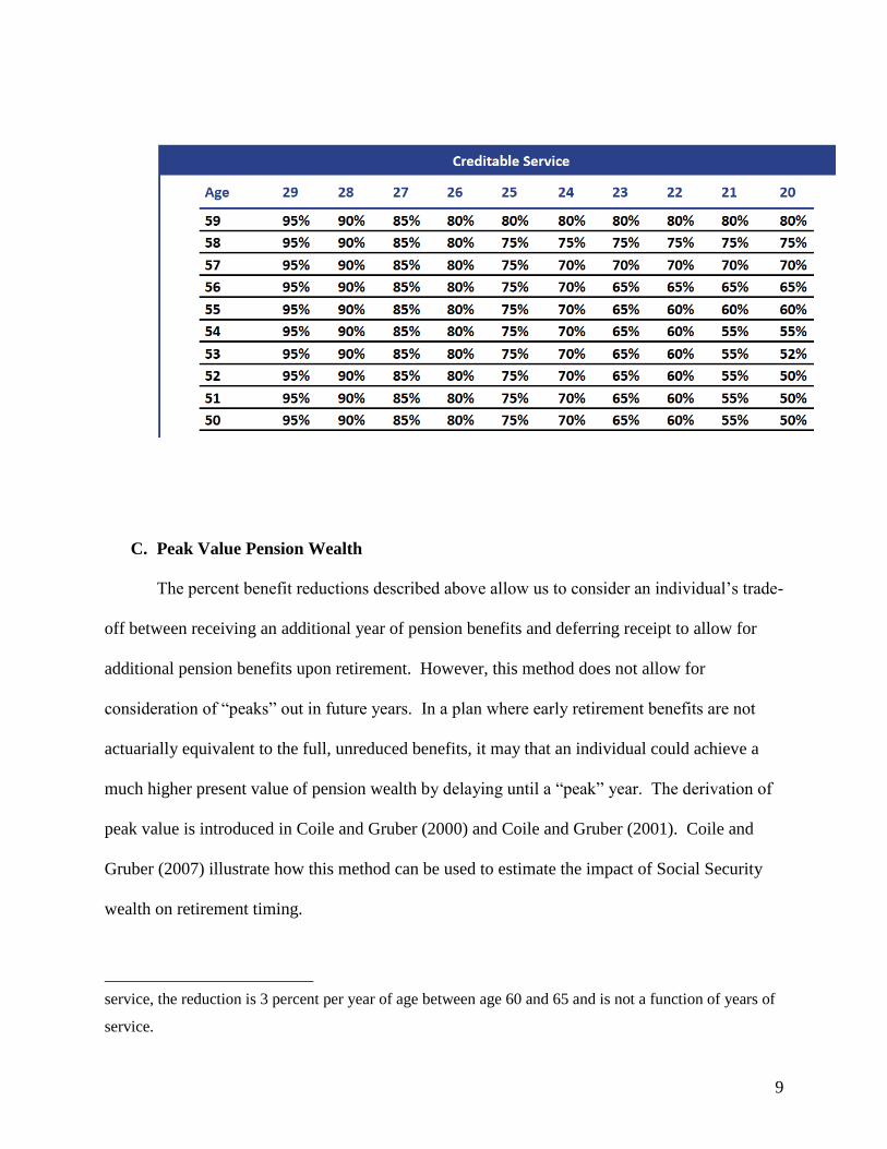
workers in TSERS and 0.0185 for workers in LGERS. Early is an early retirement reduction
factor that is imposed for an individual claiming benefits prior to attaining the age and service
requirements for unreduced benefits. See the chart below for reductions for individuals claiming
benefits between 50 and 59. Notice that the early retirement benefit is a function of both age at
claiming and years of service. For individuals aged 60 to 64 with less than 25 years of service,
there is a 3 percent per year reduction relative to the maximum benefit. The reduction factor is a
function of claiming age and the number of years the retiree is short of qualifying for unreduced
benefits.6 Thus, for many public employees in North Carolina, these plans provide a strong
economic incentive to retire in their 50’s.
TSERS formula is 1.82 percent of final average salary per year of service. Final average salary is
determined by the four highest consecutive years of earnings.
6 For most employees, Early between 50 and 59 is one minus the lesser of 5 percent per year prior to 30
years of service and is not a function of age while for persons aged 60 to 64 with fewer than 25 years of
9
C. Peak Value Pension Wealth
The percent benefit reductions described above allow us to consider an individual’s trade-
off between receiving an additional year of pension benefits and deferring receipt to allow for
additional pension benefits upon retirement. However, this method does not allow for
consideration of “peaks” out in future years. In a plan where early retirement benefits are not
actuarially equivalent to the full, unreduced benefits, it may that an individual could achieve a
much higher present value of pension wealth by delaying until a “peak” year. The derivation of
peak value is introduced in Coile and Gruber (2000) and Coile and Gruber (2001). Coile and
Gruber (2007) illustrate how this method can be used to estimate the impact of Social Security
wealth on retirement timing.
service, the reduction is 3 percent per year of age between age 60 and 65 and is not a function of years of
service.
10
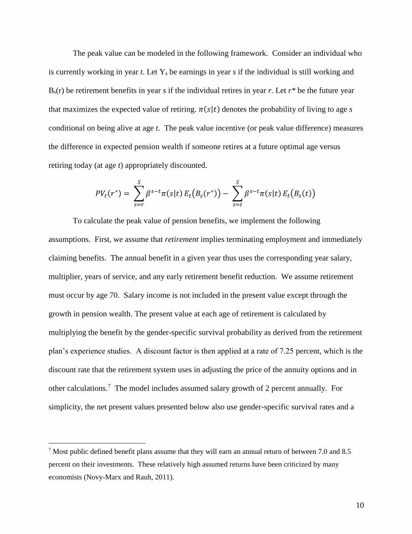
The peak value can be modeled in the following framework. Consider an individual who
is currently working in year t. Let Ys be earnings in year s if the individual is still working and
Bs(r) be retirement benefits in year s if the individual retires in year r. Let r* be the future year
that maximizes the expected value of retiring. 𝜋(𝑠|𝑡) denotes the probability of living to age s
conditional on being alive at age t. The peak value incentive (or peak value difference) measures
the difference in expected pension wealth if someone retires at a future optimal age versus
retiring today (at age t) appropriately discounted.
𝑃𝑉𝑡(𝑟∗) = ∑ 𝛽𝑠−𝑡𝜋(𝑠|𝑡)
𝑆
𝑠=𝑟
𝐸𝑡(𝐵𝑠(𝑟∗)) − ∑ 𝛽𝑠−𝑡𝜋(𝑠|𝑡)
𝑆
𝑠=𝑡
𝐸𝑡(𝐵𝑠(𝑡))
To calculate the peak value of pension benefits, we implement the following
assumptions. First, we assume that retirement implies terminating employment and immediately
claiming benefits. The annual benefit in a given year thus uses the corresponding year salary,
multiplier, years of service, and any early retirement benefit reduction. We assume retirement
must occur by age 70. Salary income is not included in the present value except through the
growth in pension wealth. The present value at each age of retirement is calculated by
multiplying the benefit by the gender-specific survival probability as derived from the retirement
plan’s experience studies. A discount factor is then applied at a rate of 7.25 percent, which is the
discount rate that the retirement system uses in adjusting the price of the annuity options and in
other calculations.7 The model includes assumed salary growth of 2 percent annually. For
simplicity, the net present values presented below also use gender-specific survival rates and a
7 Most public defined benefit plans assume that they will earn an annual return of between 7.0 and 8.5
percent on their investments. These relatively high assumed returns have been criticized by many
economists (Novy-Marx and Rauh, 2011).

11
7.25 percent discount rate. Future work will explore robustness to lower, more standard discount
rates.
Future work will implement an option value framework (Lazear and Moore 1988 and
Stock and Wise 1990) and test the sensitivity to the way that the financial incentives for
retirement are modeled.
D. Figures and Tables on Simulation
To build some intuition on how workers might respond to financial incentives, this
section reports results from simulation models of hypothetical age and years of service profiles.
The values are discounted to age 50 and assume the worker claims at a given age. The
hypothetical worker is female, a TSERS employee, with salary at entry of $35,000 regardless of
age-at-hire. We assume 2 percent earnings growth and a 7.25 percent discount rate. In Figure 1,
we observe the present value of pension wealth at each age of claiming between ages 50 and 70
by worker age-at-hire. In the first panel, we observe that a worker hired at age 24 will be eligible
for reduced benefits at ages 50 to 54 but will reach her peak of pension wealth upon reaching full
retirement eligibility at age 54. If she continues to work past 54, her annual pension benefit will
rise but she will forego those years of receiving a pension and, thus the present value of total
benefits will decline.
Similarly, a worker hired at age 34 is eligible for early retirement benefits at 20 years of
service and age 54. Each year the present value of her pension benefit rises until she reaches age
60. Since she will have 25 years of service at that time, she will be eligible for full retirement
benefits. Again, we observe that the decision to work past normal retirement eligibility results in
lower present value pension wealth. Of course, this simple model does not incorporate wage
earnings either at the current employer or at a potential outside employer. Still, the figures

12
illustrate an incentive to postpone retirement until full retirement eligibility. Further, by
comparing between the age-at-hire groups, we notice two important differences. First, the total
value of the pension is nearly twice as large for those hired at age 24 relative to those hired at age
34. Second, the “return” to waiting until full eligibility is the same in percentage terms (because
the early retirement reduction factor is the same) but the total dollar value difference is higher for
those in the younger age-at-hire group. Thus, we anticipate that more workers in this younger
age-at-hire group will wait for normal retirement than workers in the older age-at-hire group.
When an individual decides whether to retire in a given year, she must consider the peak
value of pension wealth discounted back to the current age. So, it is not enough that a future
total value is higher if she must then wait many years to receive that benefit. For a worker hired
at age 24, her present value of pension at retirement is clearly higher when calculated at age 54
than at age 50. Although discounting these values back to age 50 closes the gap, we observe that
even at age 50 the present value of her retirement wealth is higher by waiting 4 years to retire
($316,464 versus $281,132). On the other hand, the worker hired at age 34 faces a more
complicated decision. Her pension wealth is higher if she chooses to wait to claim until age 64.
However, once discounting back in time, the present value of her pension wealth will peak at age
60. We also again observe that the dollar value return to waiting is higher for the woman hired at
age 24 relative to the woman hired at age 34.
These simulations suggest that for those hired prior to age 30, most will claim when
eligible for full benefits at 30 years of service. For this group, that will occur prior to age 60.
Once controlling for benefit eligibility, any differences observed in retirement hazards by current
age can be attributed to either salience or the effect of Social Security and/or Medicare
eligibility. On the other hand, for those hired in their 30’s, early retirement may yield a higher
13
present value of lifetime pension wealth under certain assumptions regarding discounting. We
predict that many in this group will choose to retire under reduced benefits. Further, those hired
at age 35 will be eligible for full retirement benefits at age 60, those hired at age 36 will be
eligible for full retirement benefits at age 61, etc. until age 65. Controlling for full retirement
eligibility, we should not observe “excess” retirements at key eligibility ages for Social Security
or Medicare. However, we do anticipate many in this age-at-hire group will be retiring in their
early 60’s.
III. Background on the North Carolina Retirement Transitions Study
Our data are derived from survey responses linked to administrative records maintained
by the North Carolina Retirement System Division (RSD). The sample consists of public sector
workers in a large state, North Carolina, which is diverse in terms of economic activity,
urbanicity, and demographic characteristics. On most dimensions, North Carolina is broadly
representative of the nation in terms of its size, the diversity of the population, and the structure
of its public pension plans. Public sector jobs cover a wide range of occupations, skill levels,
educational backgrounds, and levels of compensation. There are over 400,000 state and local
government employees in North Carolina including doctors, lawyers, teachers and other
professional employees along with clerical and other office workers, maintenance staff,
construction workers, and law enforcement officers. The population including in our analysis is
representative of other state and local government employees and also resembles much of the
national labor force. The Retirement System Division of the Office of the State Treasurer
manages both plans. Public employees in North Carolina are also covered by Social Security
and Medicare.

14
The sample includes active workers who were ages 50-64 in March 2014. The regression
sample is organized into person-year observations where year 1 is from April 2014 through
March 2015 and year 2 is from April 2015 through March 2016. One significant limitation of
these data is that we do not observe the universe of retirements. Our data are “left censored” in
the sense that many people will have retired prior to March 2014. Thus, we conduct our
empirical estimation in a hazard model framework which allows, theoretically, for both left and
right censoring.
The data are derived from a survey of public sector workers merged with corresponding
administrative records maintained by the North Carolina Retirement Systems Division. The
administrative records contain detailed information about each employee including earnings, job
information, agency type, years of service, age, and creditable service. From these values, we
impute a projected years of service that accounts for the typical profile of purchased years of
service at retirement.8 We observe basic demographic information in the administrative data,
and we supplement this demographic information with responses to survey questions about
race/ethnicity, education level, and marital status, as well as various questions about their
spouses’ characteristics (if applicable).9
Here, we consider only those hired between ages 22-39. Future work will explore
retirement patterns for those hired after age 40. Table 2 presents descriptive statistics for the two
categories of age-at-hire. Those hired in their 20’s have an average salary of $60,219, while
those hired in their 30’s have an average salary in 2013 of $48,295. The average tenure is 25 and
8 The data appendix explains how purchased years of service is imputed.
9 The data appendix describes the data and sample in more detail. As described there, we conducted both
an email and postal mail survey. All respondents were given the option to enter a drawing for two iPad
tablets ($500 value) as an incentive for survey completion. Our response rate was approximately 18%.
15
15 years of service, respectively. The bottom portion of the table considers retirement eligibility
as of March 2016. For the younger age-at-hire group, all workers are eligible for retirement with
about 37 percent eligible for full retirement benefits. About 58% of workers hired ages 30-39
are eligible for retirement by March 2016. The regression estimates below restrict attention only
to those eligible for retirement.
The administrative data allow us to calculate a “projected” years of service by adding
typical amounts of purchased service to the observed values of earned membership years of
service. In addition, we calculate the pension values using the plan-specific survival
probabilities by gender from the plans’ own experience studies. These data are complemented
by a survey conducted in March 2014. Although that sample is not large, it is roughly
representative of the population in the administrative records. As shown in Table 2, the samples
are similar along most dimensions. Our survey sample is slightly higher earning and more likely
to be female. Importantly, the survey sample is more likely to have retired by March 2016. This
could reflect a willingness to respond to a survey as one is approaching retirement. Future work
will confirm that receiving a survey did not alter retirement behavior.
IV. Results
A. Descriptive results
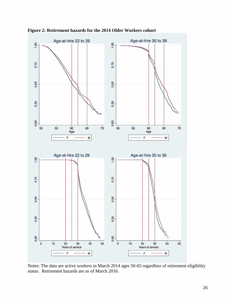
First, we consider graphically the retirement hazards separately by the two age-at-hire
groups. When consider survival by age, we observe that for both age-at-hire groups retirement
probabilities are smooth with slight drops at age 62 and 66. For those hired between ages 22-29,
we observe a sharp drop in survival at exactly 30 years of service. In contrast, there is a smaller
drop at 20 and 25 years of service for those hired in their 30’s. Those hired in their 30’s will
reach early retirement eligibility at 20 years of service. Those hired ages 30-35 will reach full

16
retirement eligibility at age 60 with between 25 and 30 years of service. For those hired between
ages 36-39, they will reach full retirement eligibility at 25 years of service between ages 61 and
64. These incentives are clearly reflected in a drop in survival at age 60 and then a gradual drop
until age 65.
Figure 3 illustrates these points using an alternative approach. These graphs consider
those that did retire and claim benefits between April 2014 and March 2016. For those hired in
their 20’s, we observe that the majority are retiring in their 50’s with a small peak at age 62.
Note that the censoring of the data can be seen in this figure as many of those that retired under
early benefits are not included in the data. Thus, the remaining sample are more likely to be
waiting until normal retirement than the average population. About 30 percent of the age-at-hire
22-29 group are retiring with 30 years of service.
For the group hired in their 30’s, on the other hand, we observe spikes at age 60
corresponding to the earliest retirement eligibility age for this group. We also observe a spike at
age 62 but only a small age 66 difference. For years of service, we observe spikes at 20, 25, and
a small spike at 30 years of service. The spike at age 62 is not due the incentives within the
pension system. Workers hired between ages 30-34 will reach full retirement eligibility at age
60 with 25 years of service. Workers hired between ages 35-39 reach early retirement eligibility
at age 60 with fewer than 25 years of service but achieve 25 years between 61-64.
B. Main regression analysis
We estimate retirement hazards for those eligible to retire under full or reduced benefits
separately by age-at-hire group. First, we include indicators for the retirement benefit reduction
level the worker would receive if retiring at her current age and years of service. While this does
17
not incorporate a “forward looking” framework, it does give a reduced form approach of what
factors an individual may be considering when making the retirement decision. In Table 3,
Column (1), the percent benefit reduction values are relative to those eligible to retire under 52,
55, 60, and 65 percent benefit reductions. Of those ages 50-64 actively working in March 2014,
all workers hired between 22-29 are eligible for early retirement benefits. Thus, they have
already rejected at least one year of early retirement benefits. We observe that those reaching
full retirement eligibility at 30 years of service are 21.9 percentage points more likely to retire
than those eligible under those reduced benefit groups. We observe that, all else equal, those age
62 are 7.8 percentage points more likely to retire and those reaching age 66 are 12.8 percentage
points more likely to retire relative to those age 55 in the data.
Table 3, Column (2) shows percent benefit reduction for people hired in their 30’s. Here
the omitted category is eligible for retirement under a 50 percent benefit reduction. We observe
a relatively flat pattern of between 9 and 18 percentage point higher probability of retirement for
those eligible for reduced benefits increasing in the percent of the benefit received. At full
benefit eligibility workers are 25 percentage points more likely to retire. We again observe that,
controlling for retirement benefit eligibility, those age 62 are 9 percentage points more likely to
retire than those age 55. However, we observe that other ages in the 60’s also have similar
differences relative to age 55.
An alternative way of framing financial incentives is to collapse these percent benefit
reduction categories into an indicator for early versus normal retirement eligibility. In the odd
columns of Table 4, we see the same basic pattern as above for each age-at-hire group.
Eligibility for normal retirement is associated with a 17 percentage point (or 109 percent of the
mean) higher probability of retirement for those hired between ages 22-29. Similarly, for those
18
hired in their 20’s, being eligible for normal retirement is associated with a 10 percentage point
higher risk of retirement, or about 94 percent of the mean. Again, the age patterns suggest some
excess retirements at key Social Security eligibility ages for the younger group but a relatively
flat age effect for the older age-at-hire group.
Next, we incorporate the peak value framework described in above. The even numbered
columns of Table 4 presents these results. Again, these estimates suggest a similar pattern.
Those hired in their 20’s and still working in their 50’s are highly responsive to the financial
incentive to wait until full retirement. Those hired in their 30’s, however, are less influenced.
C. Heterogeneity
Next, we explore heterogeneity along characteristics we can measure for the full sample
in the administrative data. The results for the younger age-at-hire group are presented in Table
5A, and those for the older age-at-hire group are presented in Table 5B. First, we explore
differences by retirement system. Workers covered by TSERS are included in the State Health
Plan (SHP) and are eligible for a relatively generous retiree health insurance benefit (see Clark,
Morrill, and Vanderweide 2014). LGERS workers are covered by employer-provided health
insurance but may not have similar retiree health insurance available. For the younger age-at-
hire group we do observe that workers covered under LGERS have a higher retirement risk at
age 65, but this pattern is not observed for the older age-at-hire group.
Next, we explore differences by men and women. For the younger age-at-hire group, we
observe that women are 18 percentage points more likely to retire under normal benefits, or 115
percent of the mean. For men hired between ages 22-29, we observe a 14.1 percentage point
higher risk of retirement once eligible for normal benefits or about 97 percent of the sample
mean. For women hired in their 30’s, being eligible for full retirement benefits is associated with
19
a 10.1 percentage point higher risk of retirement, or 91 percent of the sample mean, while for
men in this age group normal benefit eligibility is associated with 9.8 percentage point higher
retirement risk (102 percent of the sample mean).
We observe an interesting pattern by salary in 2013. Salary can reflect liquidity
constraints or outside earnings potential. For example, Brown et al. (2010) show that wealth
shocks can induce retirement. For the younger age-at-hire group, those earning less than
$50,000 per year were 14.8 percentage points more likely to retire under normal benefits or 112
percent of the sample mean. But for the older age-at-hire group, those earning less than $50,000
per year had an 8.5 percentage point higher risk of retirement under normal benefits, or only 84
percent of the sample mean. For those earning at least $50,000 annually, in the younger age-at-
hire group eligibility for normal retirement benefits is associated with an 18 percentage point
higher risk of retirement or 108 percent of the sample mean. The pattern is similar for the older
age-at-hire group. In other words, the lower earners are more sensitive to the differences in
financial incentives by age-at-hire group. Women are slightly more responsive, men seem more
likely to wait until age 66. However, these results do not account for the censoring of
retirements for the younger age-at-hire group.
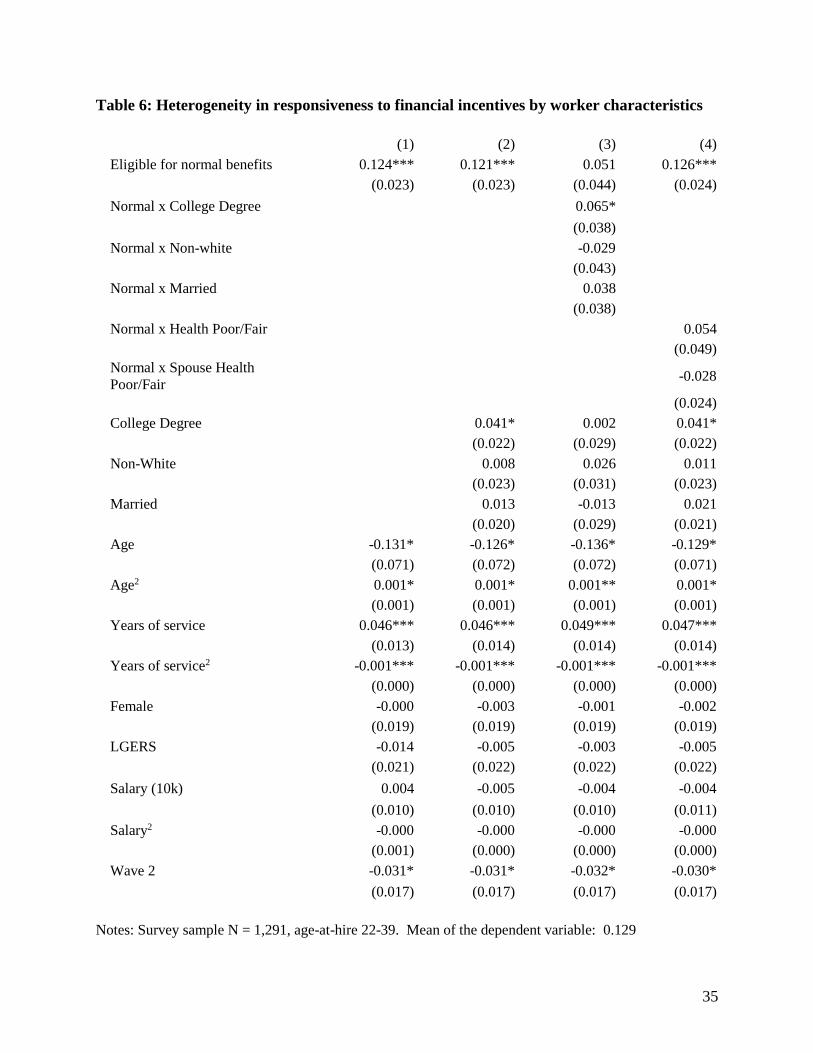
D. Survey data
While the main results using administrative records confirm that individuals are
responsive to financial incentives, on average, we anticipate underlying heterogeneity by such
characteristics as marital status, health, life expectancy, or personal discount rates. To explore
this, we turn to our smaller sample of survey respondents. The first column of Table 6 reports
estimates for a parallel specification to confirm results are similar in our smaller sample. Note
20
that we do not have enough data to estimates age fixed effects so are now including age as a
quadratic. As above, we observe that eligibility for normal retirement is associated with a 12.4
percentage point higher rate of retirement (or about 96 percent of the mean of 0.129). In column
(2) we add some basic demographic characteristics: college degree, non-white, and married. The
estimated coefficient on eligibility for normal retirement benefits is not changed when more
detailed demographics are included in the model. This provides evidence that the financial
incentives are not reflecting an omitted variable. When interacting normal retirement eligibility
with these individual characteristics, we observe that those with a college degree are significantly
more likely to retire under normal rather than early benefits.
We anticipate an important role for the health of the worker and her spouse in the timing
of retirement (e.g., McGarry 2004). We explore heterogeneity by self-reported own and spousal
health but do not detect any statistically significant differences. Future work will explore
heterogeneity along alternative dimensions including primary versus secondary earner status, the
retirement status of one’s spouse, financial literacy, stated preferences about risk and time, and a
variety of other measures. For example, Coile (2004) found that men are responsive to wives’
financial incentives but women are less responsive to husbands’ financial incentives. The detail
in our survey will allow us to explore this relationship further with respect to retirement timing
among North Carolina public sector workers.
V. Work in Progress
Workers hired in their 40’s face a distinct incentive structure. All workers are eligible for
a full benefit at age 65 with at least 5 years of service. In addition, workers with 25 years of
service are eligible for normal retirement after age 60. Otherwise, workers hired after age 40
would be first eligible for a reduced benefit at age 60. The early retirement reduction factor is

21
calculated beginning at 88% at age 60 and increases linearly by age in months at a rate of 1/4th a
percentage point per month until age 65 regardless of years of service (if vested). Future work
will model the retirement timing choices of these workers.
We anticipate receiving another wave of administrative records in December 2017 that
will provide retirement status as of November 2017. This will allow us to model retirements
over 3.5 years. In addition, we will explore more detail available in surveys conducted in March
2014 as well as a follow-up survey in March 2016.
In the spring of 2016, we gathered data from both the original survey respondents and a
“refresher” sample of individuals not original included in our survey sample. At this time, many
workers in the 2014 Older Workers cohort were already retired. Thus, we have data for both
active workers and retirees. Future work will incorporate this additional data. In the survey, we
ask individuals about Social Security claiming behavior as well. These data may allow us to
examine how individuals align pension and Social Security claiming decisions.
VI. Conclusions
A worker nearing retirement eligibility may desire to continue working either to stay
active or to earn additional income to ensure a higher standard of living. However, financial
incentives inherent in defined benefit pension systems may push workers out of the labor force at
ages that are younger than may be optimal from the workers’ and/or employers’ perspective.
This study contributes to a long literature illustrating that workers do respond to the financial
incentives inherent in their pension plans. We observe some “excess” retirements at age 62 and
66, consistent with additional incentives for retirement from Social Security eligibility ages.
This study reports findings from a new dataset that combines both survey responses and
administrative records. One key strength of this approach is that we have a much more precise

22
measure of the actual financial incentives that workers face. We consider whether certain groups
are more responsive to these incentives. Preliminary work has not revealed strong patterns in
responsiveness to financial incentives.
23
References
Asch, B., Haider, S. J., & Zissimopoulos, J. (2005). Financial incentives and retirement: evidence
from federal civil service workers. Journal of public Economics, 89(2), 427-440.
Brown, J. R., Coile, C. C., & Weisbenner, S. J. (2010). The effect of inheritance receipt on
retirement. The Review of Economics and Statistics, 92(2), 425-434.
Brown, K. M. (2013). The link between pensions and retirement timing: Lessons from California
teachers. Journal of Public Economics, 98, 1-14.
Chalmers, J., and Reuter, J. 2012. “How do retirees value life annuities? Evidence from public
employees,” The Review of Financial Studies, 25(8): 2601-2634.
Chan, Sewin and Ann Huff Stevens. 2008. “What you don’t know can’t help you: Pension
knowledge and retirement decision-making,” The Review of Economics and Statistics,
90(2): 253-266.
Clark, R., & McDermed, A. (1986). Earnings and Pension Compensation: The Effect of
Eligibility. The Quarterly Journal of Economics, 101(2), 341-361.
Clark, R. L., Morrill, M. S., & Vanderweide, D. (2014). The effects of retiree health insurance plan
characteristics on retirees’ choice and employers’ costs. Journal of health economics, 38,
119-129.
Coile, C. (2004). Retirement Incentives and Couples' Retirement Decisions. Topics in Economic
Analysis & Policy, 4(1).
Coile, C., & Gruber, J. (2007). Future social security entitlements and the retirement decision. The
Review of Economics and Statistics, 89(2), 234-246.
Costrell, R. M., & Podgursky, M. (2009). Peaks, cliffs, and valleys: The peculiar incentives in
teacher retirement systems and their consequences for school staffing. Education, 4(2),
175-211.
Fitzpatrick, M. D. (2015). How Much Are Public School Teachers Willing to Pay for Their
Retirement Benefits?. American Economic Journal: Economic Policy, 7(4), 165-188.
24
Koedel, C., & Xiang, P. B. (2017). Pension Enhancements and the Retention of Public
Employees. ILR Review, 70(2), 519-551.
Lazear, E. P., & Moore, R. L. (1988). Pensions and turnover. In Pensions in the US Economy
(pp. 163-190). University of Chicago Press.
McGarry, Kathleen. 2014. “Health and retirement: Do changes in health affect retirement
expectations?” Journal of Human Resources, 39(3): 624-648.
Novy-Marx, Robert and Joshua Rauh. 2011. “Policy options for state pension systems and their
impact on plan liabilities,” Journal of Pension Economics and Finance, 10(2): 173-194.
Shoven, John and Sita Slavov. 2014a. “Does It Pay to Delay Social Security?” Journal of
Pension Economics and Finance, 13(2): 121-144.
Shoven, John and Sita Slavov. 2014b. “Recent Changes in the Gains from Delaying Social
Security,” Journal of Financial Planning, 27(3): 32-41.
Stock, J. H., & Wise, D. A. (1990). The pension inducement to retire: An option value analysis.
In Issues in the Economics of Aging (pp. 205-230). University of Chicago Press, 1990.

25
Figure 1: Illustration of Peak Value of pension wealth
Notes: Present values are all discounted to age 50 assuming the worker claims at the given age.
The individual is assumed to be female, a TSERS employee, salary at entry=$35,000. Earnings
growth=2%, discount rate=7.25%. Peak value for age-at-hire 24 is age 54 and equivalent to
$316,464. Peak value for age-at-hire 34 is age 60 and equivalent to $150,731.
26
Figure 2: Retirement hazards for the 2014 Older Workers cohort
Notes: The data are active workers in March 2014 ages 50-65 regardless of retirement eligibility
status. Retirement hazards are as of March 2016.

27
Figure 3: Retiree characteristics by age-at-hire
Notes: The sample includes workers from the 2014 Older Workers cohort ages 50-69 who retired
before March 2016. The left panels are for age-at-hire 22-29 year olds and the right panels are
age-at-hire 30-39 year olds.

28
Table 1 Present value pension wealth for hypothetical workers by age-at-hire
Age-at-
hire
Retirement
age
Percent of
the full
benefit level
Annual
Benefit
Present value of
the pension at
retirement
Present value of
the pension at
age 50
24 50 80% $1,885 $281132 $281132
24 54 100% $2,942 $422,004 $316,464
34 54 55% $885 $126,936 $95,190
34 60 100% $2,355
$312,923 $150,731
34 64 100% $2,942 $366,137 $129,778
Notes: Comparison of the value of the pension benefit at given ages at retirement by age-at-hire
for a hypothetical workers. The values are calculated assuming the worker is female, a member
of the TSERS retirement plan, starting salary of $35,000, earnings growth rate of 2%, a discount
rate of 7.25%, and gender-specific survival probabilities derived from the plans’ experience
studies. The bolded rows are the “peak value” of the pension benefit when discounted to age 50.

29
Table 2: Person-level sample means
Administrative Records Survey Data Merged with
Administrative Records
Age-at-hire
22-29
Age-at-hire
30-39
Age-at-hire
22-29
Age-at-hire
30-39
(1) (2) (3) (4)
Number of Workers 13,591 27,234 277 417
Measured in April 2014
Age at Hire 26.147 35.488 26.134 35.261
Years of Service at Age 50 24.953 15.456 24.995 15.718
Age when eligible for
unreduced retirement benefits 56.952 62.076 56.904 61.936
Female 0.625 0.688 0.653 0.710
Total salary (2013) in '000s 60.219 48.295 64.808 55.374
City 0.087 0.078 0.058 0.098
County 0.111 0.120 0.126 0.101
Public School 0.449 0.455 0.419 0.405
General govt. 0.149 0.137 0.144 0.120
DOT 0.049 0.043 0.076 0.050
Other 0.156 0.167 0.177 0.225
Measured in March 2016
Eligible for retirement 1.000 0.578 1.000 0.686
Eligible only for early
retirement 0.634 0.419 0.657 0.477
Eligible for normal retirement 0.366 0.159 0.343 0.209
Retired by March 2016 0.288 0.138 0.343 0.170
Retired under early benefits 0.052 0.045 0.072 0.041
Retired under normal benefits 0.236 0.093 0.271 0.129
Notes: Data include all active workers ages 50-65 with no withdrawn service or breaks in service
as of March 2014 with age-at-hire as indicated. Retirement eligibility and retirement behavior
are measured as of March 2016. The survey was conducted in March 2014.

30
Table 3: Retirement timing hazard as a function of benefit eligibility rules Age-at-hire 22-29 Age-at-hire 30-39 (1) (2) Percent Benefit Reduction: Omitted Groups (50-65%) (50%)
52% 0.052
(0.037)
55% 0.093***
(0.027)
60% 0.100***
(0.027)
65% 0.081***
(0.028)
70% -0.017 0.097***
(0.031) (0.029)
75% -0.019 0.106***
(0.031) (0.030)
80% -0.005 0.110*** (0.032) (0.031)
85% -0.015 0.116*** (0.034) (0.033)
88% 0.136*** (0.035)
90% 0.010 0.141*** (0.036) (0.034)
91% 0.168*** (0.036)
94% 0.148*** (0.040)
95% or 97% 0.066* 0.176*** (0.038) (0.035)
Eligible for normal benefits 0.219*** 0.248***
(0.042) (0.035)
Age 51 -0.021 -0.003 (0.014) (0.022)
Age 52 -0.009 0.011 (0.010) (0.013)
Age 53 0.006 -0.018 (0.009) (0.014)
Age 54 0.003 0.002 (0.009) (0.012)
Age 56 0.010 0.014 (0.009) (0.011)
Age 57 0.018* 0.007 (0.010) (0.012)
Age 58 0.000 0.015

31
(0.011) (0.013)
Age 59 0.007 0.021 (0.011) (0.013)
Age 60 0.019 0.057*** (0.013) (0.016)
Age 61 -0.007 0.036** (0.015) (0.017)
Age 62 0.078*** 0.090*** (0.016) (0.017)
Age 63 0.044** 0.080*** (0.020) (0.018)
Age 64 0.022 0.056*** (0.023) (0.018)
Age 65 0.031 0.072*** (0.027) (0.019)
Age 66 0.128*** 0.089*** (0.039) (0.022)
(Projected) Years of service 0.026 -0.007 (0.019) (0.008)
(Projected) Years of service2 -0.000 0.000 (0.000) (0.000)
Female 0.012*** 0.013***
(0.005) (0.003)
LGERS -0.025*** -0.008** (0.006) (0.004)
Salary (10K) -0.007*** -0.007***
(0.002) (0.001)
Salary (10K)2 0.000 0.000
(0.000) (0.000)
Wave 2 0.001 -0.006**
(0.004) (0.003)
Number of Observations 25,194 35,266
Mean of Dependent Variable 0.155 0.106
Notes: The dependent variable is retiring in that year. The data are person-year observations. For column (1),
percent benefit reductions are relative to the omitted categories of 50, 52, 55, and 60 percent benefit reductions
because the full sample is eligible for at least some benefits. For Column (2), the percent benefit reductions
are relative to being eligible for 50% of benefits. Significance: .01 - ***; .05 - **; .1 - *;

32
Table 4: Retirement timing as a function of distance from peak value Age-at-hire 22-29 (N = 25,194) Age-at-hire 30-39 (N=35,268) (1) (2) (3) (4)
Eligible normal retirement 0.169*** 0.100***
(0.008) (0.006)
Peak value difference -0.057*** -0.008*** (0.007) (0.002)
Age 51 -0.015 -0.007 -0.023 -0.008 (0.013) (0.014) (0.019) (0.020)
Age 52 -0.004 0.004 -0.007 0.005 (0.010) (0.010) (0.012) (0.013)
Age 53 0.008 0.015* -0.029** -0.022* (0.009) (0.009) (0.012) (0.013)
Age 54 0.004 0.007 -0.002 0.002 (0.009) (0.009) (0.011) (0.011)
Age 56 0.010 0.008 0.005 -0.003 (0.009) (0.009) (0.010) (0.010)
Age 57 0.020** 0.018* 0.009 -0.006 (0.010) (0.010) (0.009) (0.010)
Age 58 0.001 0.010 0.026*** 0.005 (0.011) (0.011) (0.009) (0.009)
Age 59 0.004 0.018 0.037*** 0.014 (0.011) (0.012) (0.009) (0.009)
Age 60 0.014 0.022* 0.086*** 0.106*** (0.013) (0.013) (0.009) (0.009)
Age 61 -0.013 -0.013 0.070*** 0.091*** (0.015) (0.016) (0.009) (0.010)
Age 62 0.075*** 0.071*** 0.129*** 0.153*** (0.016) (0.017) (0.009) (0.010)
Age 63 0.042** 0.031 0.115*** 0.146*** (0.020) (0.020) (0.010) (0.010)
Age 64 0.024 0.008 0.089*** 0.123*** (0.023) (0.023) (0.011) (0.012)
Age 65 0.039 0.019 0.104*** 0.135*** (0.027) (0.027) (0.012) (0.013)
Age 66 0.144*** 0.121*** 0.122*** 0.149*** (0.038) (0.039) (0.017) (0.017)
(Projected) Years of service 0.073*** 0.084*** 0.011* 0.023*** (0.011) (0.018) (0.006) (0.006)
(Projected) Years of service2 -0.001*** -0.001*** -0.000 -0.000*** (0.000) (0.000) (0.000) (0.000)
Female 0.012*** 0.018*** 0.012*** 0.015*** (0.005) (0.005) (0.003) (0.003)
LGERS -0.025*** -0.025*** -0.008** -0.007** (0.006) (0.006) (0.004) (0.004)
Mean Dependent Variable 0.155 0.106
Notes: Dependent variable is having retired and claimed pension benefits within the year. The data are
person-year observations. Estimates are marginal effects from a probit model. The specifications include
quadratic salary and a wave 2 indicator. Significance: .01 - ***; .05 - **; .1 - *;

33
Table 5A: Heterogeneity in responsiveness to financial incentives Age-at-hire 22-29
TSERS LGERS Women Men Salary
<$50K
Salary
$50K+ (1) (2) (3) (4) (5) (6)
Eligible normal retirement 0.186*** 0.112*** 0.184*** 0.141*** 0.148*** 0.180*** (0.010) (0.016) (0.010) (0.014) (0.012) (0.011) Age 51 -0.020 0.008 -0.033* 0.011 -0.022 -0.011 (0.016) (0.025) (0.018) (0.020) (0.020) (0.018) Age 52 -0.002 -0.009 -0.002 -0.008 -0.045*** 0.018 (0.011) (0.019) (0.012) (0.016) (0.016) (0.012) Age 53 0.010 -0.003 -0.000 0.021 0.004 0.011 (0.010) (0.018) (0.011) (0.015) (0.014) (0.011) Age 54 0.002 0.008 -0.008 0.022 -0.007 0.010 (0.010) (0.017) (0.011) (0.015) (0.014) (0.011) Age 56 0.014 -0.001 0.006 0.018 0.010 0.011 (0.011) (0.018) (0.012) (0.015) (0.015) (0.012) Age 57 0.010 0.049*** 0.014 0.030* 0.019 0.022* (0.011) (0.019) (0.012) (0.016) (0.016) (0.012)
Age 58 -0.006 0.023 -0.007 0.017 0.013 -0.002 (0.012) (0.021) (0.014) (0.017) (0.017) (0.014) Age 59 0.002 0.012 0.004 0.009 -0.001 0.012 (0.013) (0.022) (0.014) (0.019) (0.018) (0.014)
Age 60 0.006 0.049** 0.021 0.010 0.033 0.012 (0.015) (0.025) (0.016) (0.020) (0.021) (0.016) Age 61 -0.018 0.018 -0.017 -0.002 -0.023 -0.002 (0.018) (0.030) (0.020) (0.024) (0.027) (0.019) Age 62 0.066*** 0.111*** 0.064*** 0.091*** 0.114*** 0.070*** (0.019) (0.030) (0.022) (0.024) (0.028) (0.020) Age 63 0.038 0.077** 0.036 0.059** 0.108*** 0.030 (0.023) (0.037) (0.026) (0.030) (0.036) (0.024) Age 64 0.022 0.044 0.058** -0.024 0.087** 0.017 (0.026) (0.046) (0.029) (0.038) (0.041) (0.028) Age 65 0.018 0.114** 0.068** 0.003 0.135*** 0.022 (0.032) (0.047) (0.035) (0.041) (0.048) (0.032) Age 66 0.175*** 0.039 0.132** 0.162*** 0.251*** 0.130*** (0.045) (0.081) (0.053) (0.056) (0.082) (0.045)
(Projected) Years of service 0.073*** 0.081*** 0.074*** 0.072*** 0.088*** 0.086***
(0.013) (0.021) (0.014) (0.017) (0.017) (0.016)
(Projected) Years of
service2 -0.001*** -0.001*** -0.001*** -0.001*** -0.001*** -0.001***
(0.000) (0.000) (0.000) (0.000) (0.000) (0.000)
Female 0.015*** 0.004 -0.030*** 0.033***
(0.005) (0.009) (0.007) (0.006)
LGERS -0.031*** -0.017** -0.028*** -0.017**
(0.008) (0.008) (0.008) (0.007)
Observations 19,481 5,713 15,678 9,516 8,295 16,899
Mean Dependent Variable 0.164 0.125 0.160 0.146 0.132 0.166

34
Table 5B: Heterogeneity in responsiveness to financial incentives Age-at-hire 30-39 TSERS LGERS Women Men Salary <$50K Salary $50K+ (1) (2) (3) (4) (5) (6)
Eligible normal retirement 0.105*** 0.079*** 0.101*** 0.098*** 0.085*** 0.121*** (0.007) (0.013) (0.008) (0.011) (0.008) (0.010)
Age 51 -0.032 -0.009 -0.029 -0.009 -0.015 -0.040 (0.024) (0.033) (0.025) (0.032) (0.023) (0.037)
Age 52 0.005 -0.051* -0.014 0.009 -0.013 0.003 (0.014) (0.028) (0.015) (0.022) (0.015) (0.021)
Age 53 -0.021 -0.053** -0.045*** 0.003 -0.026* -0.038* (0.014) (0.025) (0.015) (0.021) (0.014) (0.022)
Age 54 0.005 -0.020 -0.005 0.006 -0.006 0.004 (0.012) (0.021) (0.013) (0.020) (0.013) (0.018)
Age 56 0.013 -0.022 -0.002 0.021 0.006 0.000 (0.011) (0.020) (0.012) (0.018) (0.011) (0.017)
Age 57 0.013 -0.003 0.010 0.006 0.010 0.005 (0.011) (0.018) (0.011) (0.018) (0.011) (0.017)
Age 58 0.033*** 0.004 0.018* 0.045*** 0.015 0.043*** (0.010) (0.018) (0.011) (0.017) (0.011) (0.015)
Age 59 0.046*** 0.009 0.036*** 0.042** 0.035*** 0.040*** (0.010) (0.018) (0.011) (0.017) (0.011) (0.015)
Age 60 0.092*** 0.070*** 0.086*** 0.088*** 0.084*** 0.086*** (0.010) (0.017) (0.011) (0.017) (0.011) (0.015)
Age 61 0.078*** 0.043** 0.074*** 0.062*** 0.061*** 0.076*** (0.011) (0.019) (0.011) (0.018) (0.012) (0.016)
Age 62 0.135*** 0.116*** 0.132*** 0.127*** 0.138*** 0.119*** (0.011) (0.019) (0.011) (0.018) (0.012) (0.016)
Age 63 0.125*** 0.084*** 0.119*** 0.111*** 0.121*** 0.108*** (0.012) (0.020) (0.012) (0.019) (0.013) (0.017)
Age 64 0.096*** 0.075*** 0.101*** 0.070*** 0.086*** 0.090*** (0.013) (0.022) (0.014) (0.020) (0.015) (0.018)
Age 65 0.112*** 0.089*** 0.117*** 0.084*** 0.092*** 0.113*** (0.014) (0.024) (0.015) (0.022) (0.017) (0.019)
Age 66 0.117*** 0.137*** 0.118*** 0.130*** 0.141*** 0.107*** (0.020) (0.031) (0.022) (0.028) (0.023) (0.026)
(Projected) Years of service 0.011 0.011 0.011 0.007 0.017* 0.006
(0.007) (0.013) (0.008) (0.010) (0.009) (0.010)
(Projected) Years of service2 -0.000 -0.000 -0.000 -0.000 -0.000* -0.000
(0.000) (0.000) (0.000) (0.000) (0.000) (0.000)
Female 0.013*** 0.009 0.001 0.023***
(0.004) (0.007) (0.005) (0.005)
LGERS -0.012** -0.004 -0.010** -0.002
(0.005) (0.006) (0.005) (0.006)
Observations 27,220 8,048 23,689 11,579 19,639 15,629
Mean Dependent Variable 0.108 0.100 0.111 0.096 0.101 0.113
Notes: Dependent variable is having retired within the year. Observations are person-years. Estimates
are marginal effects from a probit model. The specifications include a quadratic in years of service,
quadratic salary, and a wave 2 indicator. Significance: .01 - ***; .05 - **; .1 - *;
35
Table 6: Heterogeneity in responsiveness to financial incentives by worker characteristics
(1) (2) (3) (4)
Eligible for normal benefits 0.124*** 0.121*** 0.051 0.126*** (0.023) (0.023) (0.044) (0.024)
Normal x College Degree 0.065*
(0.038)
Normal x Non-white -0.029
(0.043)
Normal x Married 0.038
(0.038)
Normal x Health Poor/Fair 0.054 (0.049)
Normal x Spouse Health
Poor/Fair -0.028
(0.024)
College Degree 0.041* 0.002 0.041* (0.022) (0.029) (0.022)
Non-White 0.008 0.026 0.011 (0.023) (0.031) (0.023)
Married 0.013 -0.013 0.021 (0.020) (0.029) (0.021)
Age -0.131* -0.126* -0.136* -0.129* (0.071) (0.072) (0.072) (0.071)
Age2 0.001* 0.001* 0.001** 0.001* (0.001) (0.001) (0.001) (0.001)
Years of service 0.046*** 0.046*** 0.049*** 0.047*** (0.013) (0.014) (0.014) (0.014)
Years of service2 -0.001*** -0.001*** -0.001*** -0.001*** (0.000) (0.000) (0.000) (0.000)
Female -0.000 -0.003 -0.001 -0.002 (0.019) (0.019) (0.019) (0.019)
LGERS -0.014 -0.005 -0.003 -0.005 (0.021) (0.022) (0.022) (0.022)
Salary (10k) 0.004 -0.005 -0.004 -0.004
(0.010) (0.010) (0.010) (0.011)
Salary2 -0.000 -0.000 -0.000 -0.000 (0.001) (0.000) (0.000) (0.000)
Wave 2 -0.031* -0.031* -0.032* -0.030* (0.017) (0.017) (0.017) (0.017)
Notes: Survey sample N = 1,291, age-at-hire 22-39. Mean of the dependent variable: 0.129
36
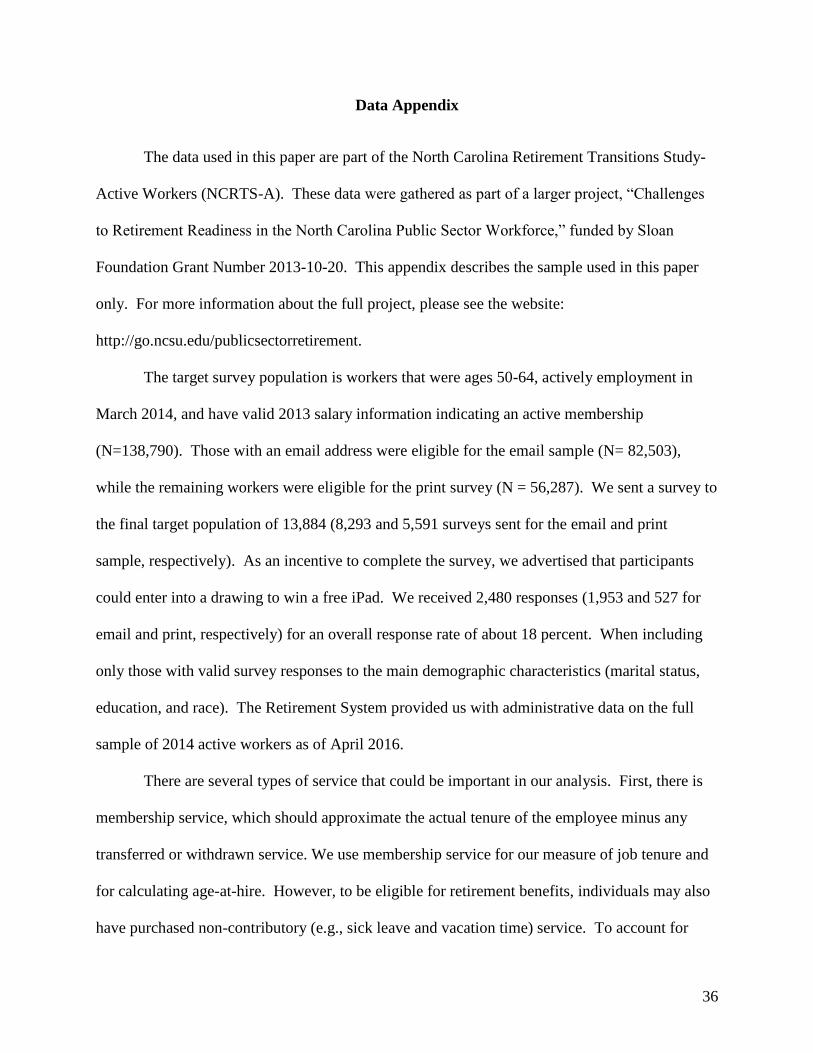
Data Appendix
The data used in this paper are part of the North Carolina Retirement Transitions Study-
Active Workers (NCRTS-A). These data were gathered as part of a larger project, “Challenges
to Retirement Readiness in the North Carolina Public Sector Workforce,” funded by Sloan
Foundation Grant Number 2013-10-20. This appendix describes the sample used in this paper
only. For more information about the full project, please see the website:
http://go.ncsu.edu/publicsectorretirement.
The target survey population is workers that were ages 50-64, actively employment in
March 2014, and have valid 2013 salary information indicating an active membership
(N=138,790). Those with an email address were eligible for the email sample (N= 82,503),
while the remaining workers were eligible for the print survey (N = 56,287). We sent a survey to
the final target population of 13,884 (8,293 and 5,591 surveys sent for the email and print
sample, respectively). As an incentive to complete the survey, we advertised that participants
could enter into a drawing to win a free iPad. We received 2,480 responses (1,953 and 527 for
email and print, respectively) for an overall response rate of about 18 percent. When including
only those with valid survey responses to the main demographic characteristics (marital status,
education, and race). The Retirement System provided us with administrative data on the full
sample of 2014 active workers as of April 2016.
There are several types of service that could be important in our analysis. First, there is
membership service, which should approximate the actual tenure of the employee minus any
transferred or withdrawn service. We use membership service for our measure of job tenure and
for calculating age-at-hire. However, to be eligible for retirement benefits, individuals may also
have purchased non-contributory (e.g., sick leave and vacation time) service. To account for

37
these latter types of service for all employees, we include an imputed amount of purchased
service. The imputation method isolated the group of individuals in the 2014 cohort who did
ultimately retire by March 2016. Of those, we calculated the actual service purchased at
retirement. Those values were collapsed into cell-specific means by gender, salary (low/high),
retirement system (TSERS/LGERS), and nine age-at-hire categories. Then, cell-specific
imputed purchased years of service is added for the full 2014 cohort to create “projected years of
service.” This method gives a more accurate measure of what benefits a worker can qualify for.
Purchased service generally includes unused vacation time and sick leave. The values range
from 1 week to 3.1 years. The average imputed purchased service is slightly over a year for the
20-29 age-at-hire group and approximately 10.5 months for the 30-39 age-at-hire group. .
Our sample is restricted to those without any withdrawn service or breaks in service.
This is necessary for us to accurately determine age-at-hire and plan benefit rules. Individuals
who have service with multiple retirement systems, that is both TSERS and LGERS can transfer
service to either retirement system at the time of claiming benefits. Hence, we restrict our
attention to individuals with membership in a single retirement system. We also exclude law
enforcement officers and any people with service in non-reciprocity retirement systems. We also
exclude a small number of workers hired prior to age 22 and those hired age 50 or later.