Retrieval of Surface Reflectance Retrieval of Surface Reflectance and LAI Mapping with Data from and LAI Mapping with Data from

ALI, Hyperion and AVIRIS ALI, Hyperion and AVIRIS

P. Gong1, G. Biging1 , R. Pu1, and M. R. Larrieu2

1Center for Assessment and Monitoring of Forest and Environmental Resources (CAMFER)

University of California, Berkeley, USA2Proyecto Forestal de Desarrollo, Secretaría de Apricultura

Buenos Aires, Argentina

ContentsContents• Objectives• Study Sites and Data• Methods• Results and Analysis• Conclusions and Remarks• Acknowledgments

ObjectivesObjectives• Develop a simple atmospheric correction

method• Map LAI with the ALI, Hyperion and AVIRIS• Examine the capabilities of the three sensors

for extracting LAI information• Compare different VI and red-edge

parameters for LAI estimation

Study Sites and DataStudy Sites and Data• Study sites:

• Two sites, in Patagonia, Argentina• Flat, semiarid region (show images)• Forest plantations, conifer species:PP, LP and Oregon P.

• Spectroradrometric measurements• ASD FieldSpec®Pro, covering 0.4 – 2.5 µm• Road surface, canopy of young plantation

• LAI measurements• 70 LAI plots, with LICOR LAI-2000 PCA• Effective LAI

Study Sites and Data Study Sites and Data (Cont(Cont’’d)d)• ALI: Advanced Land Imager

Multispectral, 9 bands, 1 panchromatic, 30 m, 3/27/2001• Hyperion: Hyperspectral Imager

• 220 bands, 0.4 – 2.5 µm• 10 nm spectral, 30 m spatial resolution, 3/27/2001

• AVIRIS: Airborne Visible/InfraRed Imaging Spectrometer• Hyperspectral sensor, altitude of 5029 m• 224 bands, 0.4 – 2.5 µm• 10 nm spectral, 3.6 m spatial resolution, 2/15/2001

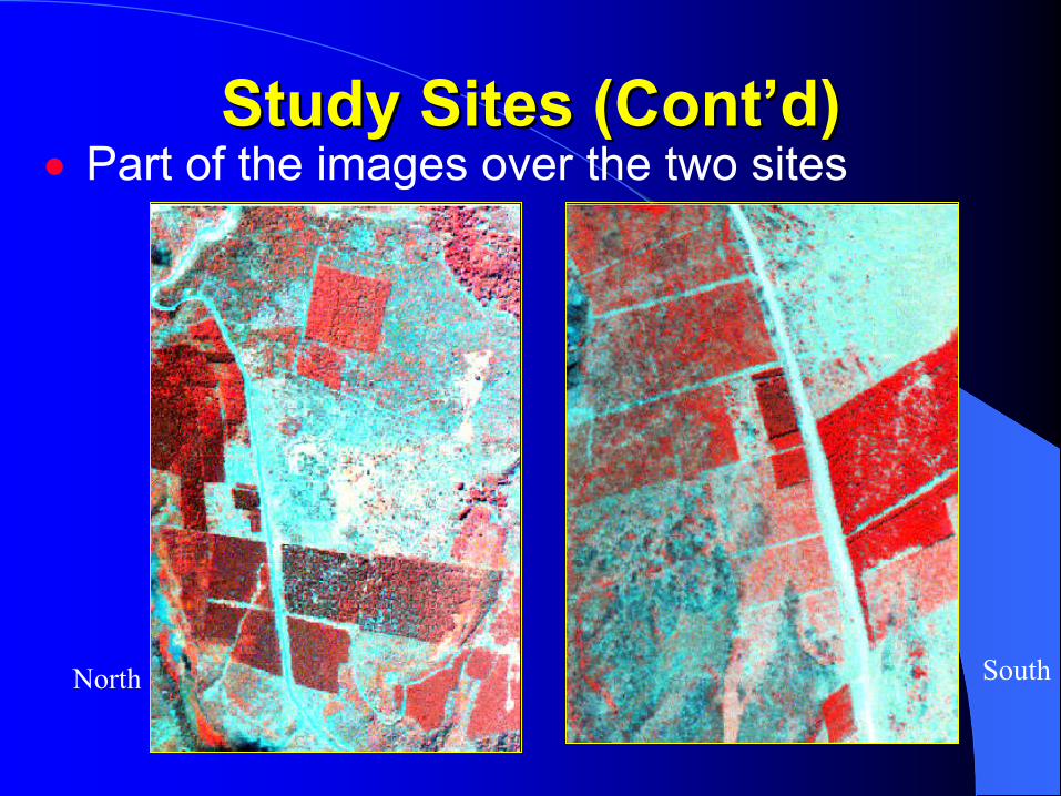
Study Sites (ContStudy Sites (Cont’’d)d)• Part of the images over the two sites

North South

MethodsMethods• Atmospheric correction

• Radiative transfer (RT) model• Radiance simulated with MODTRAN4• Retrieval surface reflectance

• LAI estimation and mapping• Correlation• LAI prediction model • LAI prediction and mapping

Atmospheric correction: A flowchart

Radiance Simulatedwith MODTRAN4

Solving RT Model

RadiativeTransfer (RT) Model

Applied to Three Sensors’ Data

Primary RetrievedReflectance

Modified Coefficients

Improved RetrievedReflectance

Radiance Simulatedwith MODTRAN4

Solving RT Model

RadiativeTransfer (RT) Model

Applied to Three Sensors’ Data

Primary RetrievedReflectance

Improved RetrievedReflectance

RT model

πθ

ρρ 002 cos

1E

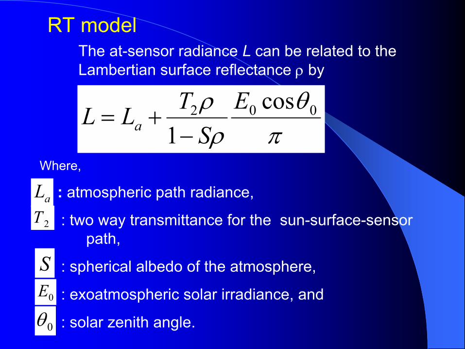
STLL a −

+=

Where,

: atmospheric path radiance,

: two way transmittance for the sun-surface-sensor path,

: spherical albedo of the atmosphere,

: exoatmospheric solar irradiance, and

: solar zenith angle.

aL2T

0E

0θ

S

The at-sensor radiance L can be related to the Lambertian surface reflectance ρ by

Radiance simulation with MODTRAN4

- Input 3 surface reflectance values: 0.0, 0.3, 0.5

- Water vapor value 0.7 cm/cm2,

- And other necessary parameters for the code

- Output total radiance

Solving RT model- To solve RT model, need 3 output total

radiances simulated with MODTRAN4.

- Solve to obtain La, T2, and S.

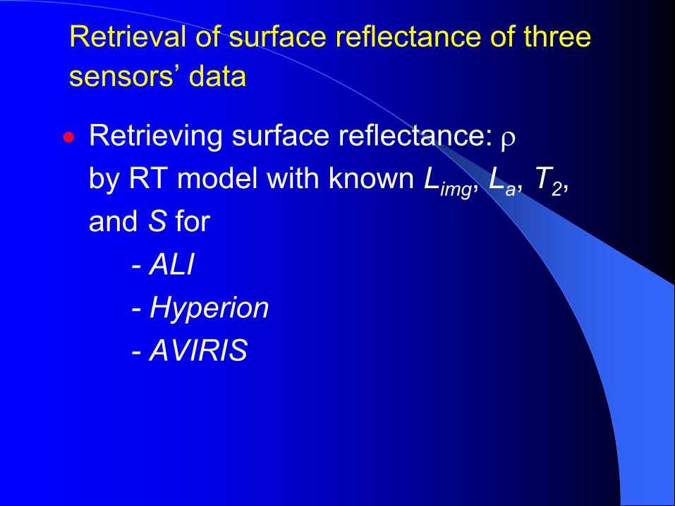
Retrieval of surface reflectance of threesensors’ data

• Retrieving surface reflectance: ρby RT model with known Limg, La, T2, and S for

- ALI- Hyperion- AVIRIS

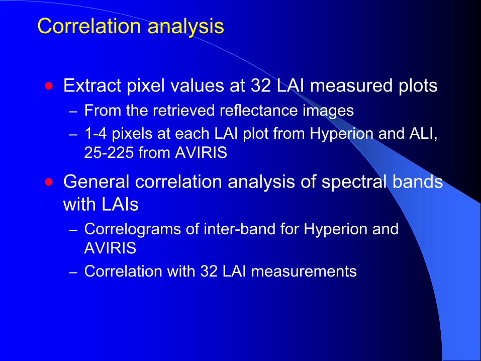
Correlation analysis

• Extract pixel values at 32 LAI measured plots– From the retrieved reflectance images– 1-4 pixels at each LAI plot from Hyperion and ALI,

25-225 from AVIRIS

• General correlation analysis of spectral bands with LAIs– Correlograms of inter-band for Hyperion and

AVIRIS– Correlation with 32 LAI measurements

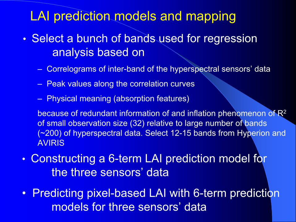
LAI prediction models and mapping• Select a bunch of bands used for regression

analysis based on– Correlograms of inter-band of the hyperspectral sensors’ data

– Peak values along the correlation curves

– Physical meaning (absorption features)

because of redundant information of and inflation phenomenon of R2

of small observation size (32) relative to large number of bands(~200) of hyperspectral data. Select 12-15 bands from Hyperion and AVIRIS

• Constructing a 6-term LAI prediction model for the three sensors’ data

• Predicting pixel-based LAI with 6-term prediction models for three sensors’ data

Results and AnalysisResults and Analysis• Three total radiances simulated• Results at different processing stages• ASD ratio coefficients• Comparison of retrieved reflectances from the

three sensors • Correlograms of inter-band of hyperspectral data• Correlation of three sensors with ALI• Determination of 6-term models• LAI prediction model (Tables)• LAI maps

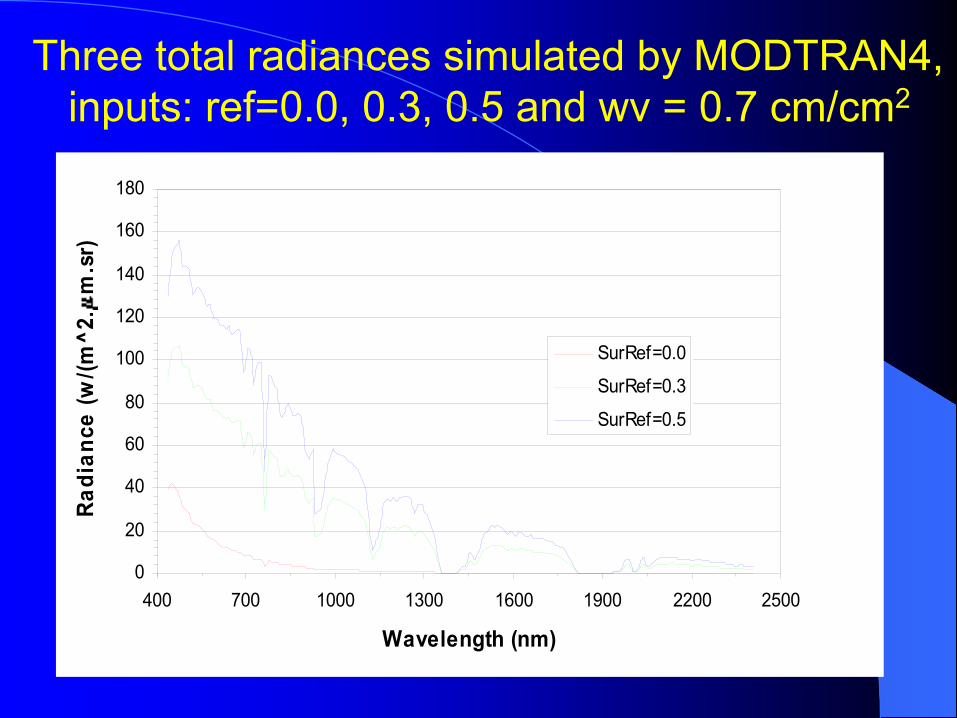
Three total radiances simulated by MODTRAN4, inputs: ref=0.0, 0.3, 0.5 and wv = 0.7 cm/cm2

0

20

40

60

80

100

120

140

160

180

400 700 1000 1300 1600 1900 2200 2500

Wavelength (nm)

Radi

ance

(w/(m

^2.

m.s

r)

SurRef=0.0

SurRef=0.3

SurRef=0.5

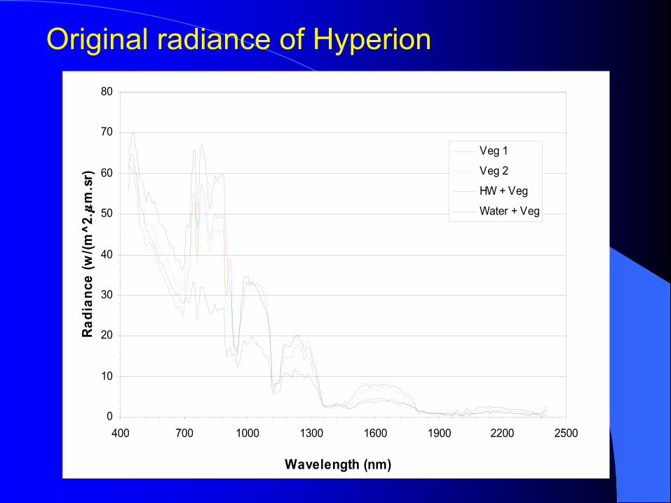
Original radiance of Hyperion

0

10

20

30

40

50

60

70

80

400 700 1000 1300 1600 1900 2200 2500

Wavelength (nm)

Radi

ance

(w/(m

^2.

m.s

r)

Veg 1

Veg 2

HW + Veg

Water + Veg

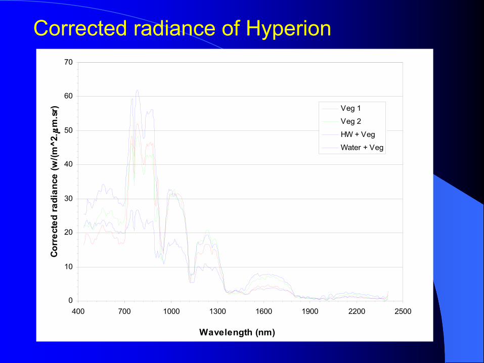
Corrected radiance of Hyperion

0

10

20

30

40

50

60

70

400 700 1000 1300 1600 1900 2200 2500

Wavelength (nm)

Corr

ecte

d ra

dian

ce (w

/(m^2

.m

.sr) Veg 1

Veg 2

HW + Veg

Water + Veg

Surface reflectance retrieved from Hyperion

0

0.1

0.2

0.3

0.4

0.5

0.6

400 700 1000 1300 1600 1900 2200 2500

Wavelength (nm)

Refle

ctan

ce

Veg 1

Veg 2

HW + Veg

Water + Veg

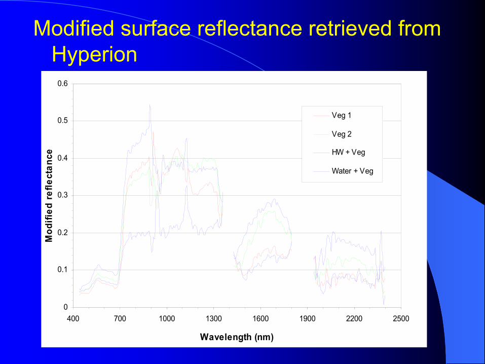
Modified surface reflectance retrieved from Hyperion

0

0.1

0.2

0.3

0.4

0.5

0.6

400 700 1000 1300 1600 1900 2200 2500

Wavelength (nm)

Mod

ified

refle

ctan

ce

Veg 1

Veg 2

HW + Veg

Water + Veg

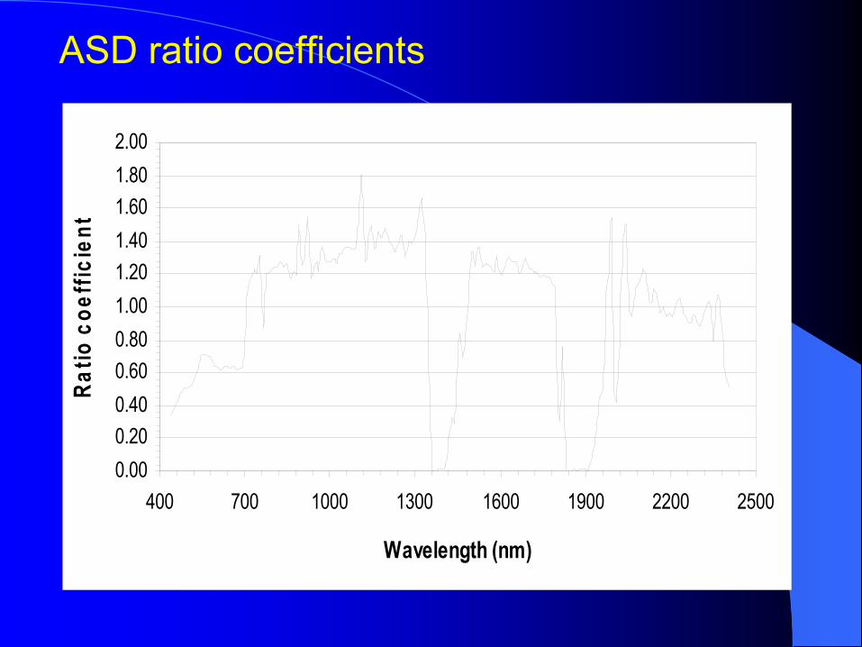
ASD ratio coefficients

0.000.200.400.600.801.001.201.401.601.802.00

400 700 1000 1300 1600 1900 2200 2500

Wavelength (nm)

Ratio

coe

ffici

ent

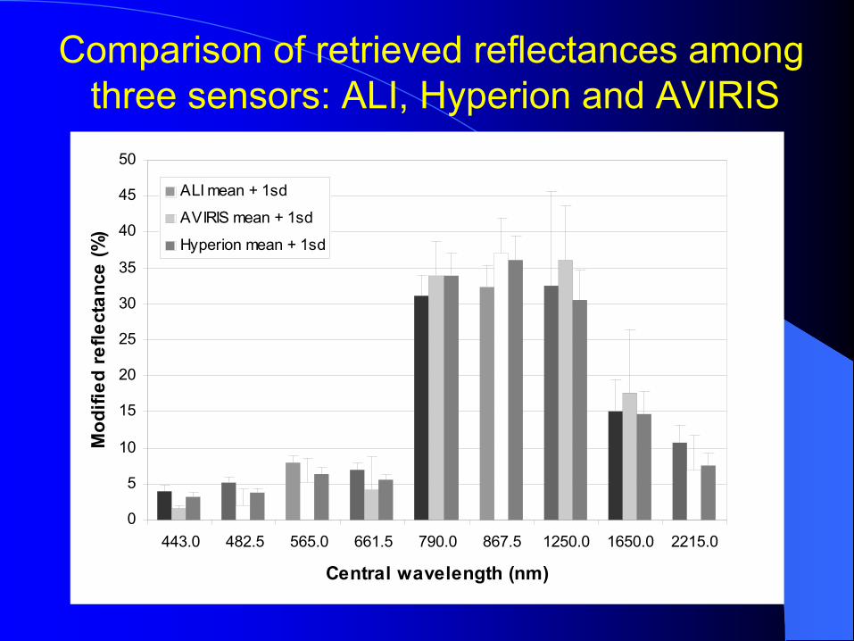
Comparison of retrieved reflectances among three sensors: ALI, Hyperion and AVIRIS

0

5

10

15

20

25

30

35

40

45

50

443.0 482.5 565.0 661.5 790.0 867.5 1250.0 1650.0 2215.0

Central wavelength (nm)

Mod

ified

refle

ctan

ce (%

)

ALI mean + 1sd

AVIRIS mean + 1sd

Hyperion mean + 1sd

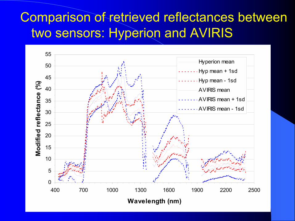
Comparison of retrieved reflectances between two sensors: Hyperion and AVIRIS

0

5

10

15

20

25

30

35

40

45

50

55

400 700 1000 1300 1600 1900 2200 2500

Wavelength (nm)

Mod

ified

ref

lect

ance

(%)

Hyperion mean

Hyp mean + 1sd

Hyp mean - 1sd

AVIRIS mean

AVIRIS mean + 1sd

AVIRIS mean - 1sd

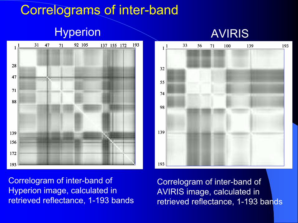
Correlograms of inter-band

7133

74

32

1

55

98

139

193

1 56 100 139 1937133

74

32

1

55

98

139

193

1 56 100 139 193

Correlogram of inter-band of AVIRIS image, calculated in retrieved reflectance, 1-193 bands

71

28

1

47

88

139

156

172

193

71311 47 92 105 137 172 193155

71

28

1

47

88

139

156

172

193

71

28

1

47

88

139

156

172

193

71311 47 92 105 137 172 19315571311 47 92 105 137 172 193155

Correlogram of inter-band of Hyperion image, calculated in retrieved reflectance, 1-193 bands

Hyperion AVIRIS

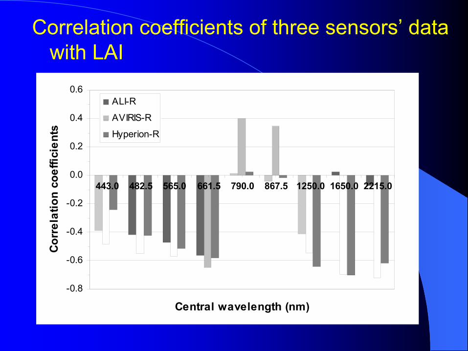
Correlation coefficients of three sensors’ data with LAI

-0.8

-0.6

-0.4

-0.2

0.0

0.2

0.4

0.6

443.0 482.5 565.0 661.5 790.0 867.5 1250.0 1650.0 2215.0

Central wavelength (nm)

Corr

elat

ion

coef

ficie

nts

ALI-R

AVIRIS-R

Hyperion-R

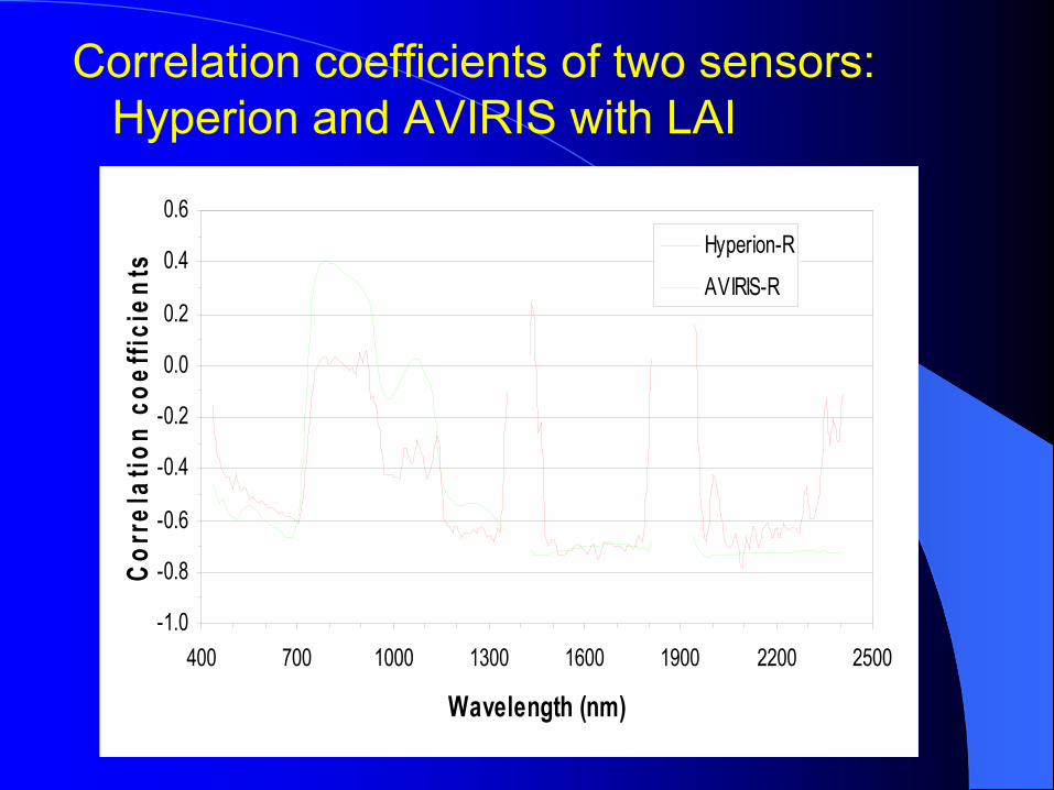
Correlation coefficients of two sensors: Hyperion and AVIRIS with LAI

-1.0

-0.8

-0.6

-0.4

-0.2

0.0

0.2

0.4

0.6

400 700 1000 1300 1600 1900 2200 2500

Wavelength (nm)

Cor

rela

tion

coef

ficie

nts Hyperion-R

AVIRIS-R

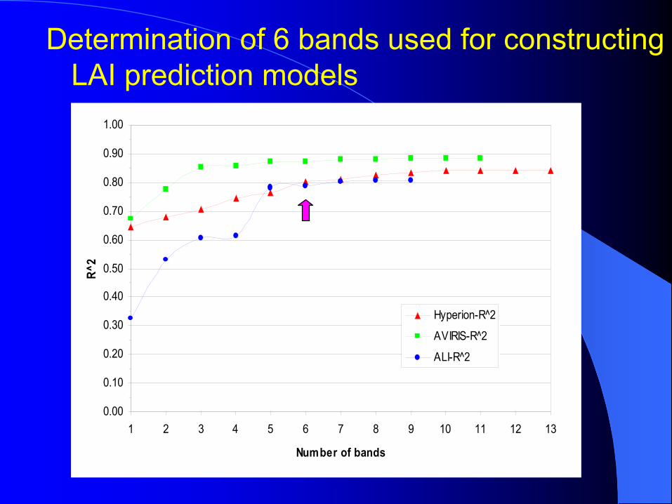
Determination of 6 bands used for constructing LAI prediction models

0.00

0.10

0.20

0.30

0.40

0.50

0.60

0.70

0.80

0.90

1.00

1 2 3 4 5 6 7 8 9 10 11 12 13

Number of bands

R^2

Hyperion-R^2

AVIRIS-R^2

ALI-R^2

0.00

0.10

0.20

0.30

0.40

0.50

0.60

0.70

0.80

0.90

1.00

1 2 3 4 5 6 7 8 9 10 11 12 13

Number of bands

R^2

Hyperion-R^2

AVIRIS-R^2

ALI-R^2

LAI prediction models using retrieved surfacereflectance data from ALI, Hyperion and AVIRISN = 32, 6 bands selected into the models.

Hyperion ALI AVIRISLog(Ref) Log(Ref) Log(Ref)

R2 0.8019 0.7884 0.8731Wavelengths 499, 913, 1437 483, 790, 868 684, 932, 1080(nm) 1639, 2093, 2275 1250, 1650, 2215 1991, 2261, 2400OAA(%) 78.56 77.82 82.83S.D. 0.5492 0.5679 0.4397

Note: OAA=overall accuracy; S.D.=standard deviation; all of R2 are significant at 0.99 confident level.

LAI

0 – 1

1 – 2

2 – 3

3 – 4

4 – 5

> 5

(d)(c)

(b)(a)

LAI

0 – 1

1 – 2

2 – 3

3 – 4

4 – 5

> 5

LAI

0 – 1

1 – 2

2 – 3

3 – 4

4 – 5

> 5

(d)(c)

(b)(a)

LAI maps, (a) pseudo-color composite of AVIRIS, (b) LAI map from AVIRIS, (c) LAI map from Hyperion and (d) LAI map from ALI

LAI maps

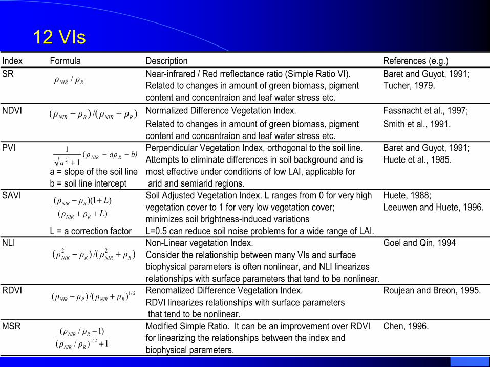
Index Formula Description References (e.g.)SR Near-infrared / Red rreflectance ratio (Simple Ratio VI). Baret and Guyot, 1991;

Related to changes in amount of green biomass, pigment Tucher, 1979.content and concentraion and leaf water stress etc.

NDVI (ρNIR-ρR)/(ρNIR+ρR) Normalized Difference Vegetation Index. Fassnacht et al., 1997;Related to changes in amount of green biomass, pigment Smith et al., 1991.content and concentraion and leaf water stress etc.

PVI Perpendicular Vegetation Index, orthogonal to the soil line. Baret and Guyot, 1991;Attempts to eliminate differences in soil background and is Huete et al., 1985.

a = slope of the soil line most effective under conditions of low LAI, applicable forb = soil line intercept arid and semiarid regions.

SAVI Soil Adjusted Vegetation Index. L ranges from 0 for very high Huete, 1988;vegetation cover to 1 for very low vegetation cover; Leeuwen and Huete, 1996.minimizes soil brightness-induced variations

L = a correction factor L=0.5 can reduce soil noise problems for a wide range of LAI.NLI Non-Linear vegetation Index. Goel and Qin, 1994

Consider the relationship between many VIs and surface biophysical parameters is often nonlinear, and NLI linearizes relationships with surface parameters that tend to be nonlinear.

RDVI Renomalized Difference Vegetation Index. Roujean and Breon, 1995.RDVI linearizes relationships with surface parameters that tend to be nonlinear.

MSR Modified Simple Ratio. It can be an improvement over RDVI Chen, 1996.for linearizing the relationships between the index and biophysical parameters.

b)aρρa

RNIR −−+

(1

12

)/()( RNIRRNIR ρρρρ +−

RNIR ρρ /

)()1)((

LρρLρρ

RNIR

RNIR

+++−

)/()( 22RNIRRNIR ρρρρ +−

2/1)/()( RNIRRNIR ρρρρ +−

1)/()1/(

2/1 +−

RNIR

RNIR

ρρρρ

12 VIs

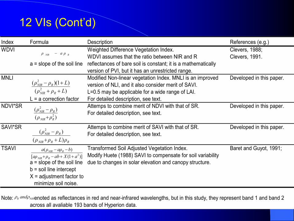
Index Formula Description References (e.g.)WDVI Weighted Difference Vegetation Index. Clevers, 1988;

WDVI assumes that the ratio between NIR and R Clevers, 1991.a = slope of the soil line reflectances of bare soil is constant; it is a mathematically

version of PVI, but it has an unrestricted range.MNLI Modified Non-linear vegetation Index. MNLI is an improved Developed in this paper.

version of NLI, and it also consider merit of SAVI.L=0.5 may be applicable for a wide range of LAI.

L = a correction factor For detailed description, see text.NDVI*SR Attemps to combine merit of NDVI with that of SR. Developed in this paper.

For detailed description, see text.

SAVI*SR Attemps to combine merit of SAVI with that of SR. Developed in this paper.For detailed description, see text.

TSAVI Transformed Soil Adjusted Vegetation Index. Baret and Guyot, 1991; Modify Huete (1988) SAVI to compensate for soil variability

a = slope of the soil line due to changes in solar elevation and canopy structure.b = soil line interceptX = adjustment factor to minimize soil noise.

Note: denoted as reflectances in red and near-infrared wavelengths, but in this study, they represent band 1 and band 2across all avaliable 193 bands of Hyperion data.

RNIR a ρρ −

)()1)((

2

2

LρρLρρ

RNIR

RNIR

+++−

)()(

2

2

RNIR

RNIR

ρρρρ

+−

RRNIR

RNIR

ρLρρρρ

)()( 2

++−

)]1([)(

2aXabρaρbaρρa

RNIR

RNIR

++−+−−

NIRR andρρ

12 VIs (Cont’d)

Three approaches (Cont’d)• Polynomial fitting (in fifth order)

∑=

+=5

10

i

iiλaaρ

−−−−= 2

20

0 2exp)

σλ)(λ)R(RRR(λ ss

• IG red edge model, linear fitting with least square solution (Miller et al., 1990)

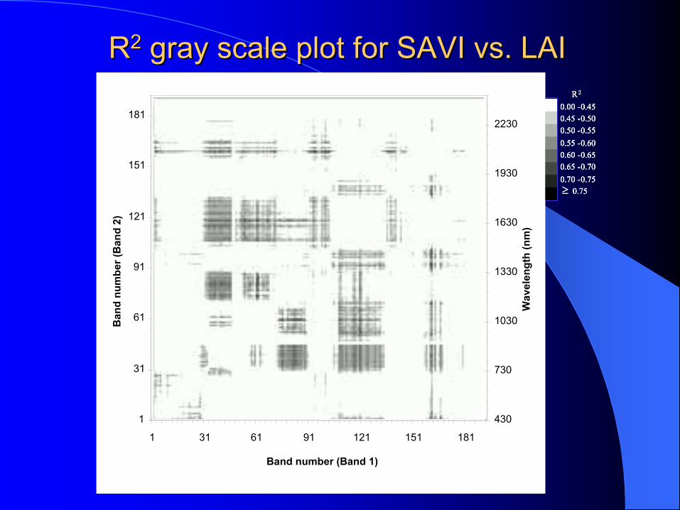
RR22 gray scale plot for SAVI vs. LAIgray scale plot for SAVI vs. LAI

0.00 -0.450.45 -0.500.50 -0.550.55 -0.600.60 -0.650.65 -0.700.70 -0.75

0.75

R2

≥

1

31

61

91

121

151

181

1 31 61 91 121 151 181

Band number (Band 1)

Ban

d nu

mbe

r (B

and

2)

430

730

1030

1330

1630

1930

2230

Wav

elen

gth

(nm

)

0.00 -0.450.45 -0.500.50 -0.550.55 -0.600.60 -0.650.65 -0.700.70 -0.75

0.75

R 2

≥

0.00 -0.450.45 -0.500.50 -0.550.55 -0.600.60 -0.650.65 -0.700.70 -0.75

0.75

R 2

≥

1

31

61

91

121

151

181

1 31 61 91 121 151 181

Band number (Band 1)

Ban

d nu

mbe

r (B

and

2)

430

730

1030

1330

1630

1930

2230

Wav

elen

gth

(nm

)

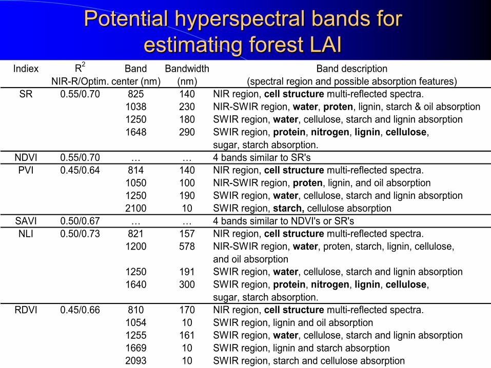
Potential hyperspectral bands for Potential hyperspectral bands for estimating forest LAIestimating forest LAI

Indiex R2 Band Bandwidth Band descriptionNIR-R/Optim. center (nm) (nm) (spectral region and possible absorption features)

SR 0.55/0.70 825 140 NIR region, cell structure multi-reflected spectra.1038 230 NIR-SWIR region, water, proten, lignin, starch & oil absorption1250 180 SWIR region, water, cellulose, starch and lignin absorption1648 290 SWIR region, protein, nitrogen, lignin, cellulose,

sugar, starch absorption.NDVI 0.55/0.70 … … 4 bands similar to SR'sPVI 0.45/0.64 814 140 NIR region, cell structure multi-reflected spectra.

1050 100 NIR-SWIR region, proten, lignin, and oil absorption1250 190 SWIR region, water, cellulose, starch and lignin absorption2100 10 SWIR region, starch, cellulose absorption

SAVI 0.50/0.67 … … 4 bands similar to NDVI's or SR'sNLI 0.50/0.73 821 157 NIR region, cell structure multi-reflected spectra.

1200 578 NIR-SWIR region, water, proten, starch, lignin, cellulose, and oil absorption

1250 191 SWIR region, water, cellulose, starch and lignin absorption1640 300 SWIR region, protein, nitrogen, lignin, cellulose,

sugar, starch absorption.RDVI 0.45/0.66 810 170 NIR region, cell structure multi-reflected spectra.

1054 10 SWIR region, lignin and oil absorption1255 161 SWIR region, water, cellulose, starch and lignin absorption1669 10 SWIR region, lignin and starch absorption2093 10 SWIR region, starch and cellulose absorption

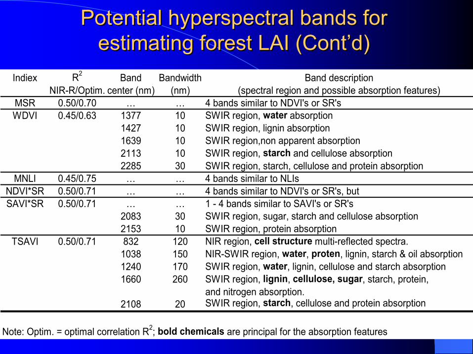
Potential hyperspectral bands for Potential hyperspectral bands for estimating forest LAI (Cont’d)estimating forest LAI (Cont’d)

Indiex R2 Band Bandwidth Band descriptionNIR-R/Optim. center (nm) (nm) (spectral region and possible absorption features)

MSR 0.50/0.70 … … 4 bands similar to NDVI's or SR'sWDVI 0.45/0.63 1377 10 SWIR region, water absorption

1427 10 SWIR region, lignin absorption1639 10 SWIR region,non apparent absorption2113 10 SWIR region, starch and cellulose absorption2285 30 SWIR region, starch, cellulose and protein absorption

MNLI 0.45/0.75 … … 4 bands similar to NLIsNDVI*SR 0.50/0.71 … … 4 bands similar to NDVI's or SR's, but SAVI*SR 0.50/0.71 … … 1 - 4 bands similar to SAVI's or SR's

2083 30 SWIR region, sugar, starch and cellulose absorption2153 10 SWIR region, protein absorption

TSAVI 0.50/0.71 832 120 NIR region, cell structure multi-reflected spectra.1038 150 NIR-SWIR region, water, proten, lignin, starch & oil absorption1240 170 SWIR region, water, lignin, cellulose and starch absorption1660 260 SWIR region, lignin, cellulose, sugar, starch, protein,

and nitrogen absorption.2108 20 SWIR region, starch, cellulose and protein absorption

Note: Optim. = optimal correlation R2; bold chemicals are principal for the absorption features

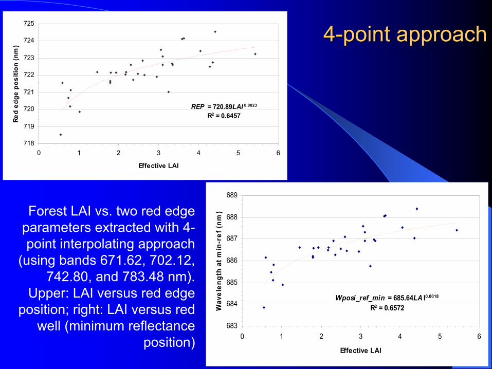
44--point approachpoint approach

REP = 720.89LAI 0.0023

R2 = 0.6457

718

719

720

721

722

723

724

725

0 1 2 3 4 5 6

Effective LAI

Red

edge

pos

ition

(nm

)

Wposi_ref_min = 685.64LA I0.0018

R2 = 0.6572

683

684

685

686

687

688

689

0 1 2 3 4 5 6

Effective LAI

Wav

elen

gth

at m

in-r

ef (n

m)Forest LAI vs. two red edge

parameters extracted with 4-point interpolating approach

(using bands 671.62, 702.12, 742.80, and 783.48 nm).

Upper: LAI versus red edge position; right: LAI versus red

well (minimum reflectance position)

ConclusionsConclusions• The method of atmospheric correction used in this

study is promising but needs refinement.• LAI prediction model derived from AVIRIS has the

highest correlation and lowest regression SD, followed by Hyperion and ALI

• Since atmospheric effects on VNIR more than SWIR, more potential in SWIR with Hyperion.

• Atmospheric correction is critical for hyperspectral data application, especially in VNIR region

Conclusions contConclusions cont’’dd• Most of the important bands with high R2 related to bands in

SWIR region and some in NIR region. • The bands centered near 820, 1040, 1200, 1250, 1370,

1430, 1650, 2100, 2260 nm with bandwidths from 10 to 300 nm are important for constructing VIs for estimating LAI.

• The 4-point approach is a more practical application method to extract two red edge parameters because only 4 bands are considered for use

• It is notable that the originally defined VIs with R and NIR bands did not produce higher correlation with LAI than VIs constructed with bands in SWIR region.

• Atmospheric correction is critical for hyperspectral data application, especially for VNIR region

AcknowledgmentsAcknowledgments• This research was supported by a NASA

EO-1 science validation grant (NCC5-492) and field support provided by the forest plantation inventory section of the agricultural department of the government of Argentina.

• Assistance in field work by Gillsermo Defossé, Florencia Farias, and Maria Cristina Frugoni is appreciated.