Embed Size (px)
Citation preview

Bank of Canada staff working papers provide a forum for staff to publish work-in-progress research independently from the Bank’s Governing Council. This research may support or challenge prevailing policy orthodoxy. Therefore, the views expressed in this paper are solely those of the authors and may differ from official Bank of Canada views. No responsibility for them should be attributed to the Bank.
www.bank-banque-canada.ca
Staff Working Paper/Document de travail du personnel 2017-30
Retrieving Implied Financial Networks from Bank Balance-Sheet and Market Data
by José Fique

2
Bank of Canada Staff Working Paper 2017-30
July 2017
Retrieving Implied Financial Networks from Bank Balance-Sheet and Market Data
by
José Fique
Financial Stability Department Bank of Canada
Ottawa, Ontario, Canada K1A 0G9 [email protected]
ISSN 1701-9397 © 2017 Bank of Canada

i
Acknowledgements
I would like to thank Bo Young Chang, an anonymous referee, and the seminar
participants at the Department of Economics and Finance of the Texas State University –
San Marcos for useful comments and suggestions. All errors are mine.
ii
Abstract
In complex and interconnected banking systems, counterparty risk does not depend only
on the risk of the immediate counterparty but also on the risk of others in the network of
exposures. However, frequently, market participants do not observe the actual network of
exposures. I propose an approach that incorporates this network of exposures, among
other factors, in a valuation model of credit default swaps. The model-implied spreads are
then used to retrieve the set of networks that are consistent with market spreads. The
approach is illustrated with an application to the UK banking system.
Bank topics: Financial institutions; Financial stability
JEL codes: C63, D85, G21
Résumé
Dans les systèmes bancaires complexes et interconnectés, le risque de contrepartie ne
dépend pas uniquement du risque de la contrepartie immédiate, mais aussi du risque
d’autres agents dans le réseau d’expositions. Cependant, fréquemment, les acteurs du
marché n’observent pas le réseau réel d’expositions. Je propose une approche qui intègre
ce réseau d’expositions, entre autres facteurs, dans un modèle d’évaluation des swaps sur
défaillance de crédit. Les écarts implicites du modèle sont ensuite utilisés pour récupérer
l’ensemble des réseaux qui sont compatibles avec les écarts du marché. L’approche est
illustrée au moyen d’une application au système bancaire britannique.
Sujets : Institutions financières ; Stabilité financière
Codes JEL : C63, D85, G21

Non-Technical Summary
Banks are complex organizations that establish important economic relationships with their peers.Therefore, assessing from an isolated perspective the counterparty credit risk of a bank may fail toprovide a complete picture.
Assessing counterparty risk in a truly system-wide manner poses difficult challenges since thenetwork of economic links that ties banks together can seldom be observed by researchers and mar-ket participants. However, since this network is relevant for counterparty risk assessment, marketparticipants may need to form expectations about it, which are reflected in the market prices ofclaims issued by banks.
In this paper, I propose an approach based on a valuation model that takes into account, amongother factors, the interbank network of exposures. By comparing the model-implied prices with ob-served market prices for claims issued by banks, this approach helps allocate aggregate exposures,which can be observed from banks’ balance sheets, at a bilateral level.
This approach is then illustrated with an empirical application to the UK banking system usingdata from the 2007–09 financial crisis period. This empirical application seems to suggest that intimes of stress, market participants may find it difficult to discern the network structure of exposuresfrom the maximum uncertainty benchmark.
iii

1 Introduction
Simulations used to assess the risk of contagion in banking systems frequently include the interbanknetwork of exposures (e.g., Gauthier et al. 2012). However, with some exceptions, researchersand market participants alike cannot observe the true matrix of exposures. Nevertheless, the totalamount of exposures of a given financial institution is available from its balance sheet, albeit onlyat a relatively low frequency. Even though some information is available, this poses a missing dataproblem that affects the results of these simulations.
This paper proposes an approach to complement balance-sheet information with market datain order to enhance our understanding of the expected relevance of these exposures to marketparticipants.
Here, I propose a valuation model that takes into account not only how common exposuresaffect the balance sheets of firms, but also the impact of the network of exposures on the marketprices of contingent claims. The theoretical prices of these claims are then used to retrieve the setof networks that are consistent with observed prices.
Using an extension of the structural credit risk model of Merton (1974)1 that incorporates theimpact of contagious defaults on the market value of debt, I define the set of implied networks.These implied networks are defined as the ones that, while respecting the total amount loaned andborrowed obtained from balance-sheet information, are consistent with market data, according tothe theoretical valuation model.
This translates into a network optimization problem. I use a genetic algorithm to find thenetwork that improves upon the weighted mean squared error (WMSE) between the network-basedtheoretical and observed prices using the commonly used maximum entropy (ME) network as abenchmark.2
As Abbassi et al. (2017) show for German banks, market-based measures of interconnectednesscorrelate with the true interbank exposures. Therefore, the networks retrieved using the method thatI propose have the potential to augment other approaches, such as ME, that rely only on aggregateexposures, leading to a more accurate assessment of systemic risk.
To the best of my knowledge, this is the first paper to draw on both aggregate exposures andmarket information to simulate bilateral exposures. The contribution of this paper is an applied onethat illustrates how market information can be combined with balance-sheet information to infer thenetwork of bilateral exposures. To do so, I subject the approach to an empirical application usingdata for four UK global systemically important banks (G-SIB) referring to the 2007–09 financial
1More precisely, I use the model proposed in Elsinger et al. (2006) to value defaultable debt via Monte Carlosimulation.
2The ME approach implicitly assumes that firms wish to diversify their exposures among counterparties as muchas possible; see Upper (2011) for example.
1

crisis period based on balance sheet data retrieved from the 2008 interim (henceforth AUG2008),annual reports for 2008 (henceforth DEC2008) and 2009 (henceforth DEC2009), and correspond-ing credit default swaps (CDS) spreads.
The improvement of the WMSE over the ME benchmark varied substantially across the timeslices considered in this empirical application. While the improvement was very similar for AUG2008and DEC2009 – around 40%, it was lower for the DEC2008 slice – roughly 25%. These resultsseem to indicate that in DEC2008, market participants seemed to perceive a network of exposurescloser to the maximum uncertainty benchmark (i.e., ME).
One potential explanation is that as the level of risk increases at the aggregate level, as it canbe argued that was the case when looking at the CDS spreads for the four banks, it becomes moredifficult to discern bilateral exposures. This then leads to market participants perceiving a networkof exposures closer to the ME benchmark. Alternatively, it can be the case that since the ratioof internal (interbank) assets to total assets tends to be lower in DEC2008, the distribution ofinterbank assets across counterparties is less relevant for pricing of risk. This argument is lessstrong, however, when we notice that the ratio of interbank assets to equity tends to decline overtime and not just for the DEC2008 slice.
While theoretical support for the valuation model can be found in the literature (Fischer 2014proposes a valuation model that shares similarities with the one proposed in this paper) and theoverall approach has been used to assess systemic risk (see, for example, Elsinger et al. 2006),which is the ultimate reason to be interested in these networks, the approach does come at the costof imposing an a priori structure to the data.
The use of a modified Merton model brings with it some strong assumptions that constrain theability of the approach to accurately model market prices.
The rest of the paper is structured as follows. Section 2 frames the paper in the literature.Section 3 presents a motivating example. Section 4 describes the asset pricing model used to derivemodel-implied prices for a given network. Section 5 explains the approach used to retrieve the setof implied networks. Section 6 shows the results of simulations used to analyze the sensitivity ofthe methodology to exogenous factors. Section 7 elaborates on the motivating example providedin Section 3 to provide some intuition behind the mechanisms at play in the simulations. Section 8presents the empirical application. Finally, Section 9 concludes.
2 Literature review
This paper is related to several strands of literature. Firstly, the paper is closely related to papers thataddress the issue of reconstructing financial networks based on partial information, such as Anandet al. (2015), Anand et al. (2017), Gandy and Veraart (2016) and Montagna and Lux (2017). Even
2

though in this paper the totals of internal assets and liabilities are also key pieces of information todetermine the set of model-implied networks, this information is complemented with market-basedsignals to shed light on the market perception of the network of exposures. Secondly, since theset of model-implied networks is determined by an asset pricing model, this paper is related to theliterature on asset pricing in financial networks (see, for example, Eisenberg and Noe 2001, Egloffet al. 2007, Gouriéroux et al. 2013, Barucca et al. 2016 and Abbassi et al. 2017). Finally, the paperis also related to the literature on the potential role that uncertainty about the network of exposuresplays in financial contagion, which has been studied by Caballero and Simsek (2013) and Li et al.(2016).
While these papers focus on pricing contingent claims dependent on a true network, the focusof this paper is to search for a set of networks that reconciles model-implied and observed pricesfor those claims. The paper by Abbassi et al. (2017) closely relates to mine as the authors showthat for German banks, market-based measures of interconnectedness correlate with the interbankexposures and these vary both at a cross-sectional level and over time. Thus, the informationcontained in market prices constitutes a valuable input in reconstructing networks from partialdata.
3 A motivating example
Suppose that in a four-bank system, total internal assets and liabilities are given as follows:3
Table 1: Matrix of individually unknown exposuresA B C D Liabilities
A 0 ? ? ? 15B ? 0 ? ? 11C ? ? 0 ? 13D ? ? ? 0 10
Assets 11 18 12 8
Naturally, there is more than one matrix of exposures that is consistent with the total individualexposures displayed in Table 1. Consider, as an example, the following matrices:
3Note that by convention, the diagonal of such matrices is assumed to be a vector of zeros.
3

Table 2: Matrices consistent with aggregate exposuresA B C D Liabilities
A 0 3 8 4 15B 4 0 4 3 11C 4 8 0 1 13D 3 7 0 0 10
Assets 11 18 12 8
A B C D LiabilitiesA 0 4 8 3 15B 3 0 4 4 11C 4 8 0 1 13D 4 6 0 0 10
Assets 11 18 12 8
Even though both of these matrices are consistent with the aggregate exposures, they may implydifferent outcomes when used for risk assessment purposes, as already pointed out by Mistrulli(2011). Thus, to inform this process, I propose a model that I describe in the next section.
4 The model
In this section, I present a valuation model, which is an extension of Merton (1974), that takes intoaccount the impact of the network of exposures in the market price of defaultable debt. Funda-mentally, I use the model proposed in Elsinger et al. (2006) to value defaultable debt via MonteCarlo simulation. The model-implied (or theoretical) prices are then used to determine the set ofnetworks of exposures that are consistent with the observed prices.
The section is divided into three subsections. In Subsection 4.1, I show how the balance sheetof an interconnected firm changes according to the paths assumed for its own assets and liabilitiesand also via its connections with the value of other firms’ assets and liabilities at maturity. Then, inSubsection 4.2, I present a valuation algorithm since a closed-form expression cannot be obtained.Finally, in Subsection 4.3, I formally define the concept of the networks that are consistent withmarket data conditional on the theoretical prices derived from the valuation model4 proposed inSubsections 4.1 and 4.2.
4.1 Basic setup
Consider an industry where firms, in addition to establishing economic ties with firms in otherindustries, establish relevant connections within the same industry.5 The balance sheet of a typicalfirm i in this industry, with i ∈ I = 1, ...,n , can be decomposed into: (i) internal assets (IAi) andliabilities (ILi); (ii) external assets (EAi) and liabilities (ELi); and (iii) equity (EQi). In illustrativeterms,6
4Similar asset pricing models have already been proposed by Fischer (2014).5While the focus of this paper is on debt claims, an interesting extension would be to also treat equity claims, which
is left for future research.6Note that the decomposition of the balance sheet does not have a quantitative meaning.
4

Assets Liabilities
EAiELi
ILi
IAi EQi
TAi T Li +EQi
where total assets of firm i (TAi) are equal to the sum of EAi and IAi, and total liabilities (T Li)
are equal to the sum of ELi and ILi.
In particular, in the case of the banking industry, internal assets and liabilities can be thought ofas interbank loans and external assets as loans to the non-financial sector.
Following Elsinger et al. (2006), I assume the following dynamics for the external assets of firmi:
dEAi(t)EAi(t)
= rdt +σidZi(t),
where Zi is a one-dimensional Brownian motion defined in the filtered risk-neutral probabilityspace (Ω,P,F ,Ft), r is the risk-free rate and σi is the volatility of the assets of i. Also, r and σi
are assumed to be constant, and the instantaneous correlation between Zi(t) and Z j(t) is given byρi j for all i and j ∈ I. In its turn, the value of the internal assets at t = T is given by
IA j (T ) = ∑ni=1 p?i mi j,
where mi j is the nominal liability of firm i to firm j, the typical element of the exposure matrixM ∈M with M being the space of all possible liabilities matrices. M is assumed to remainunaltered before the common maturity date of all internal claims, and p?i is the fraction of theliabilities of firm i recovered by all other creditors with the same priority of internal claims atmaturity.7 For the purpose of the methodology developed in this paper, it is critical that there existsa class of defaultable debt with observable market prices that has the same priority in liquidation asthe bilateral exposures that I wish to retrieve. Thus, I make the following assumptions:
Assumption 1. (Seniority structure of debt) Internal liabilities (ILi) and external liabilities (ELi)
have the same priority in liquidation.
Under this assumption, I define a new liabilities matrix, M ∈ M , with M defined analogouslyto M , that summarizes the cross holdings of debt with the same priority in liquidation as the bilat-eral exposures among firms. This matrix extends M to include a (sink) node that has no liabilitiesto other nodes to accommodate the external liabilities of all other nodes and is given by
7Note that if all firms remain solvent, p? is simply a vector of ones. However, if the i−th firm is unable to repay itscreditors fully, the i−th entry of this vector is lower than one reflecting the number of cents on the dollar each creditorends up receiving.
5

1 2 ... n n+1 Liabilities
1 0 m12 ... m1n EL1 EL1 +n
∑j=1
m1 j
2 m21 0 ... m2n EL2 EL2 +n
∑j=1
m2 j
... ... ... ... ... ... ...
n mn1 mn2 ... 0 ELn ELn +n
∑j=1
mn j
n+1 0 0 ... 0 0 0
Assetsn
∑i=1
mi1
n
∑i=1
mi2 ...n
∑i=1
min
n
∑k=1
ELin+1
The formal presentation of their definition follows.Let e = EA be the firms’ external assets, di = ∑ j mi j and
⊙denote the Hadamard product.
Then, under assumptions:
Assumption 2. (Limited liability) ∀ i ∈ I, p? = max(
M′p?+ e)⊙( 1
d1, ..., 1
dn+1
),0.
Assumption 3. (Proportional repayment)
∀ i ∈ I, p? = min
1,(
M′p?+ e)⊙(
1d1
, ...,1
dn+1
),
that is, if obligations are not paid in full, then creditors obtain a proportional share of the total
value of the firm’s assets with respect to the outstanding debt.
Definition 1. The clearing payment vector is given by
p? = min
1,max(
M′p?+ e)⊙(
1d1
, ...,1
dn+1
),0
.
As Eisenberg and Noe (2001) (henceforth EN) show, this vector has some desirable properties,such as existence and uniqueness, under some regularity conditions. Even though this vector hasthe desirable property of reflecting how the successive rounds of contagious defaults affect the lossgiven default, it does not take into account the reduction in the value of the assets when a bankdefaults. For this reason, I use the extended version of the Eisenberg and Noe (2001) algorithmproposed by Rogers and Veraart (2013) that allows for a fractional loss, 1−α, realized when e isliquidated.
6

In the next subsection, I propose the valuation algorithm that determines the theoretical pricethat will be used in the subsequent subsection to define the set of networks implied by the observedprices.
4.2 Valuation via Monte Carlo simulation
Given that loss-given default is endogenously determined by the clearing payment vector, the de-faultable bonds are valued by Monte Carlo simulation. As described in Hull (Hull), assumingconstant interest rates, the price of the asset can be found by taking the following steps:
1. Sample a random path for EAi in a risk-neutral world.
2. Find p? via the fictitious default algorithm based on the sample path.
3. Repeat steps 1. and 2. K times.
4. Calculate the average of the payoff of the defaultable bond in a risk-neutral setting by com-puting the average of p? over all states of nature. Note that in this setting, p? is the recoveryrate, which is also the normalized payoff of the defaultable debt.
5. Discount the expected payoffs using the risk-free rate, r, to obtain the theoretical price ofdefaultable debt.
4.3 The set of implied networks
The entire analysis as presented thus far implicitly assumes that the network of claims is observable.However, this is only true for a reduced number of cases. In most instances, only the total amountborrowed/loaned is known. All studies based on the fictitious default algorithm are either basedon data available strictly to central banks or on reconstruction methods, such as ME, that relymostly on aggregate exposures (see Anand et al. 2017 for a comparative study on the differentreconstruction methods). Entropy maximization roughly translates into assuming that firms wishto diversify their exposures as much as possible, which may be a strong assumption with potentiallyimportant consequences for risk assessment, as pointed out by Mistrulli (2011).
A natural extension of the valuation algorithm presented in Subsection 4.2 is to use observedmarket prices to infer the network that is likely to generate them, much like the method to re-cover the option-implied volatility (see, for example, Jackwerth and Rubinstein (1996)). A possiblemethod of doing so is to minimize the WMSE between the observed and theoretical prices of a zerocoupon bond with a face value of $1 at time t with maturity T.
7

Definition 2. Let F denote the set of feasible liabilities matrices, i.e.,
F :=
M ∈ M :
n
∑k=1
mik = mi.∩n
∑k=1
mk j = m. j ∩ mii = 0 ∩ min+1 = ELi ∀ i ∈ I
,
where mi. and m. j are the total amount of internal liabilities of i and the total amount of internalassets of j, respectively. Note that mi., m. j and ELi can be observed from balance sheets, albeit ata relatively low frequency.
Definition 3. Let IN, the set of implied networks, denote the set of liabilities matrices that are asolution to Problem 1:
IN := argminM∈F
Ξ(M | θ
),
where
Ξ(M | θ
):=
1n
[pobs
t − e−r f τEQt(p?(M | θ
))]′W[
pobst − e−r f τEQ
t(p?(M | θ
))],
with
W =
TA1
∑nj=1 TA j
0 ... 0
0 TA2∑
nj=1 TA j
... 0
... ... ... 00 0 0 TAn
∑nj=1 TA j
,
θ = (EA(t) ,r,σ ,ρ)
and τ = T − t. The choice of the weighting matrix based on the relative size of a bank is justifiedby higher liquidity, and thus informativeness, of the market signal.
Alternatively, a similar expression can be derived using CDS spreads instead of bond prices.The set of implied networks is now given by
INcds := argminM∈F
Ξcds
(M | θ
), (1)
where
Ξcds(M | θ
):=
1n
cdsobst +
ln[e−r f τEQ
t(p?(M | θ
))]τ
− r f
′
W
cdsobst +
ln[e−r f τEQ
t(p?(M | θ
))]τ
− r f
.8

5 The genetic algorithm
I propose an approach based on a genetic algorithm adapted to network optimization to solve Prob-lem 1.8 The algorithm works as follows:
1. Use the ME network as a starting point.
2. Generate ngen “mutations” of the ME matrix and compute the model predicted prices. Thisset of matrices is referred to as the children set.
3. Evaluate the fitness, i.e., compute Ξ(M | θ
), for all matrices generated in 2.
4. Preserve the npar matrices with the best fitness. This set of matrices is referred to as the setof parents.
5. Create ngen “mutations” of the matrices generated in 4. and proceed as in step 2.
6. Evaluate the fitness of all matrices generated in step 4.
7. Repeat steps 4-6 until the fitness measure improves a specified percentage over the fitnessmeasure (i.e., WMSE) obtained for the ME network.
The success of the algorithm depends on the ability of each new generation to preserve the bestfitting connections of the parent matrices while “mutating” in such a way that the fitness improves.In order for this to be possible, the mutation process takes place as follows:
1. Uniformly select two parents and replace one of the nodes of parent 1 in the copy of parent 2(see Figure 1 for an illustration).
2. Add an innovation to all off-diagonal elements of each child matrix and re-balance the re-sulting matrix to ensure that total loaned/borrowed amounts are preserved.9
8Genetic algorithms have been used previously in network science to detect communities in graphs. See, forexample, Pizzuti (2008).
9This is achieved by employing the RAS algorithm; see Schneider and Zenios (1990).
9

Figure 1: Mutation process
A
B
C
D
A
B
C
D
A
B
C
D
Parent 1 Parent 2
Child 1
This figure depicts the creation of Child 1 based on Parents 1 and 2. Note that Child 1 is the result of copying Parent 1 and replacing node C’sconnections with the corresponding ones obtained from Parent 2 and then re-balancing the resulting matrix to ensure that total loaned/borrowedamounts are preserved. Additionally, the exposure of node C to nodes A and B are introduced as innovations.
6 Simulations
The model can be more easily understood with the help of some illustrative simulations that revealthe sensitivity of the results to changes in key parameters. To do so, I randomly generated 50networks that are treated as the “true” network and compared against these simulated networks theperformance of both the ME and implied (or optimized) networks approaches.10
Interbank assets were calibrated to 5% of total assets, volatility of banks’ assets ranged between2.7% and 4%, risk-free rate was set at around 2%, the minimum initial leverage ratio was set at 3%,and for each network 500 states of nature were simulated.
The following figures show the simulated cumulative distributions of the deviation of the num-ber of defaults in excess of the ones associated with the assumed network when one of the recon-structed networks (ME or optimized) is used instead.
10These 50 networks were generated separately for each comparison.
10
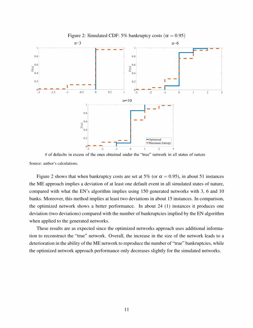
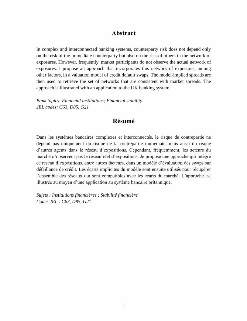
Figure 2: Simulated CDF: 5% bankruptcy costs (α = 0.95)
Source: author’s calculations.
Figure 2 shows that when bankruptcy costs are set at 5% (or α = 0.95), in about 51 instancesthe ME approach implies a deviation of at least one default event in all simulated states of nature,compared with what the EN’s algorithm implies using 150 generated networks with 3, 6 and 10banks. Moreover, this method implies at least two deviations in about 15 instances. In comparison,the optimized network shows a better performance. In about 24 (1) instances it produces onedeviation (two deviations) compared with the number of bankruptcies implied by the EN algorithmwhen applied to the generated networks.
These results are as expected since the optimized networks approach uses additional informa-tion to reconstruct the “true” network. Overall, the increase in the size of the network leads to adeterioration in the ability of the ME network to reproduce the number of “true” bankruptcies, whilethe optimized network approach performance only decreases slightly for the simulated networks.
11

Figure 3: Simulated CDF: 15% bankruptcy costs (α = 0.85)
Source: author’s calculations.
A natural question to ask is how the performance of the optimized network approach changeswhen bankruptcy costs increase. Since the network structure is likely to be more relevant whenbankruptcy costs increase, one would expect to see an increase in the gap in performance of theoptimized networks approach over ME. This is what Figure 3 confirms. When bankruptcy costsincrease from 5% to 15%, the ME (optimized network) approach produces biased results in 50%(6%) of the instances when compared with the results of the “true” network.
12
Figure 4: Simulated CDF: noisy prices for n = 6 and α = 0.95
Source: author’s calculations.
However, the effectiveness of the optimized network approach relies substantially on the abilityof market signals to convey information about the network. Since market signals are likely tocontain a noise component, the performance of the optimized network approach deteriorates as thenoise in the market signal increases.
To understand how sensitive the approach is, I added a uniformly distributed random variableto each “fundamental” price (i.e., the one that results from the application of the pricing model tothe “true” network) such that the prices used to retrieve the optimized network deviate from theaverage “fundamental” price in a specified percentage.
Figure 4 shows that when a noise term is added to the theoretical bond prices, ME can out-perform the optimized network approach. For 6 banks and 5% bankruptcy costs, the optimizednetwork approach greatly outperforms ME when noise is non-existent. However, when the noiseterm is set between -0.001% and 0.001% of the average “fundamental” price, the performance ofboth approaches is somewhat comparable. Finally, ME largely outperforms the optimized networkapproach when the noise term is between -0.01% and 0.01%.
13

7 A numerical example (revisited)
In the motivating example of Section 3, I showed that there is more than one matrix that satisfiesthe total exposures constraints. I now revisit the example to present the differences among networktopologies and predicted bond prices of the assumed “true”, ME and the implied liabilities matricesin order to provide some intuition on the simulations conducted in Section 6. The purpose of thisnumerical example is to provide some intuition on how changes in how exposures are reallocatedaffect prices.
I assume r f = 0 to make the explanation more intuitive. This allows me to match bond priceswith expected recovery rates at maturity (i.e., the Eisenberg and Noe’s clearing payment vector) foreach Monte Carlo draw. Given simulated paths for the EA(T ) vector, and assuming that the “true”liabilities matrix that results from market participants’ expectations is
A B C D Liabilities
A 0 3 8 4 15
B 4 0 4 3 11
C 4 8 0 1 13
D 3 7 0 0 10
Assets 11 18 12 8
the predicted vector of bond prices is [.8919, .8940, .9502, .9082]. However, based on the samesimulated paths for EA(T ), the predicted price vector is [.8919, .8940, .9505, .9082] when the MEnetwork is considered (left table) and [.8920, .8940, .9501, .9082] when the implied network ap-proach is used (right table):
A B C D Liabilities
A 0 7.28 4.83 2.89 15
B 4.14 0 4.29 2.57 11
C 4.08 6.38 0 2.54 13
D 2.78 4.34 2.88 0 10
Assets 11 18 12 8
A B C D Liabilities
A 0 4.89 7.20 2.91 15
B 3.64 0 4.09 3.23 11
C 4.07 7.07 0 1.86 13
D 3.25 6.04 0.71 0 10
Assets 11 18 12 8
The key takeaways are that reallocating the exposures has an effect on the prices of an instru-ment (specifically, bond prices), which can be understood as the extent to which shocks to all nodesaffect a particular node.
Under the ME network, node C is less affected by shocks to all banks than under the “true”network. Conversely, under the network retrieved using the algorithm, node C (A) is more (less)affected by shocks to all banks than under the “true” network, albeit the deviations are smaller thanthe ones under the ME network.
14
More precisely, when considering the ME matrix, the extent to which contagion affects C isunderestimated. This is the case because the ME network, in line with the implied assumptionthat firms wish to diversify their exposures as much as possible, puts relatively more weight on theexposures of C to B and D, which have a higher expected recovery value than A. Note also that thereis no significant difference in the payment vector entries for all other firms. This can be explainedas follows. First, the ME solution is almost identical to the original for the internal assets of A.
Second, even though the ME solution substantially affects the distribution of the internal claims ofB, the fact that B’s internal assets largely exceed its internal liabilities makes B’s payment vectorentry largely independent of the liabilities matrix. Finally, D’s payment vector entry also remainslargely unaltered, even though the ME approach redistributes D’s interbank assets by reducing theweight in A and B (which have low recovery value) to C (which has a high recovery value). Onepotential explanation is that the external assets of D are more than sufficient to fulfill its obligationswhen there is a default by one or more of its counterparties.
Analogously, the price vector obtained from the implied network indicates that the extentto which contagion affects firms A (C) is underestimated (overestimated). Note that under thismethodology, A’s internal assets are relatively more (less) concentrated in D (B) than under ME,thus the expected effects of contagion are less severe under the proposed methodology since theexpected recovery of D is higher than of B. However, since in the implied network C’s internal as-sets are more concentrated in A rather than in D, in contrast to the ME solution, C’s clearing vectorentry is lower than both under the ME and “true” networks.
8 Empirical application
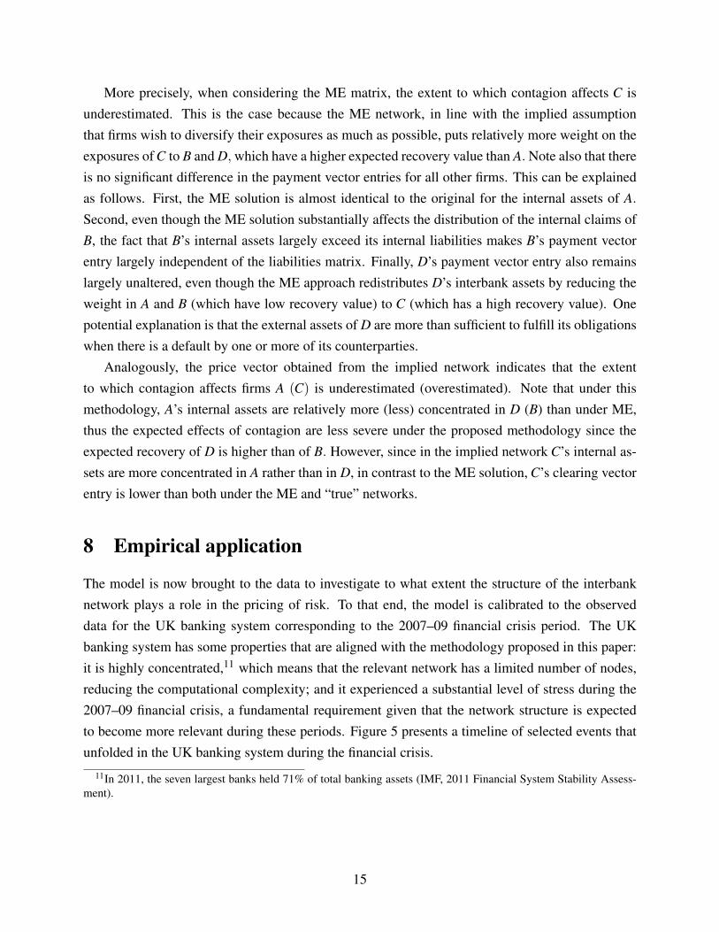
The model is now brought to the data to investigate to what extent the structure of the interbanknetwork plays a role in the pricing of risk. To that end, the model is calibrated to the observeddata for the UK banking system corresponding to the 2007–09 financial crisis period. The UKbanking system has some properties that are aligned with the methodology proposed in this paper:it is highly concentrated,11 which means that the relevant network has a limited number of nodes,reducing the computational complexity; and it experienced a substantial level of stress during the2007–09 financial crisis, a fundamental requirement given that the network structure is expectedto become more relevant during these periods. Figure 5 presents a timeline of selected events thatunfolded in the UK banking system during the financial crisis.
11In 2011, the seven largest banks held 71% of total banking assets (IMF, 2011 Financial System Stability Assess-ment).
15
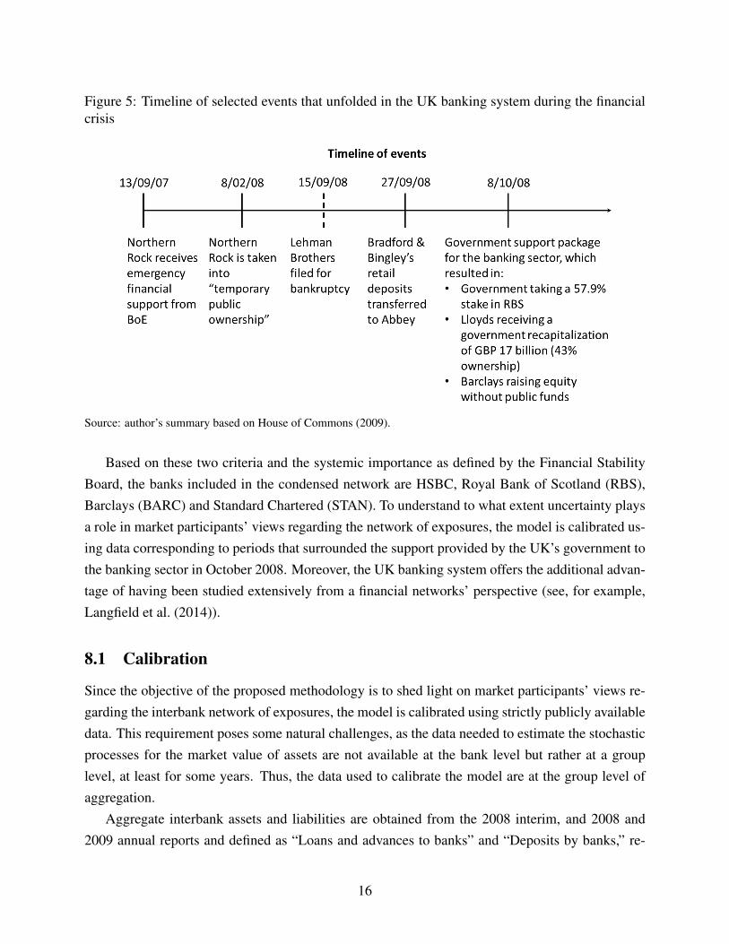
Figure 5: Timeline of selected events that unfolded in the UK banking system during the financialcrisis
Source: author’s summary based on House of Commons (2009).
Based on these two criteria and the systemic importance as defined by the Financial StabilityBoard, the banks included in the condensed network are HSBC, Royal Bank of Scotland (RBS),Barclays (BARC) and Standard Chartered (STAN). To understand to what extent uncertainty playsa role in market participants’ views regarding the network of exposures, the model is calibrated us-ing data corresponding to periods that surrounded the support provided by the UK’s government tothe banking sector in October 2008. Moreover, the UK banking system offers the additional advan-tage of having been studied extensively from a financial networks’ perspective (see, for example,Langfield et al. (2014)).
8.1 Calibration
Since the objective of the proposed methodology is to shed light on market participants’ views re-garding the interbank network of exposures, the model is calibrated using strictly publicly availabledata. This requirement poses some natural challenges, as the data needed to estimate the stochasticprocesses for the market value of assets are not available at the bank level but rather at a grouplevel, at least for some years. Thus, the data used to calibrate the model are at the group level ofaggregation.
Aggregate interbank assets and liabilities are obtained from the 2008 interim, and 2008 and2009 annual reports and defined as “Loans and advances to banks” and “Deposits by banks,” re-
16
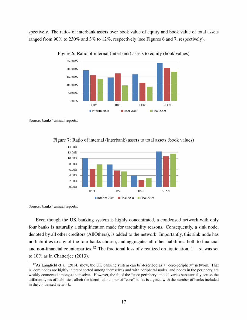
spectively. The ratios of interbank assets over book value of equity and book value of total assetsranged from 90% to 230% and 3% to 12%, respectively (see Figures 6 and 7, respectively).
Figure 6: Ratio of internal (interbank) assets to equity (book values)
Source: banks’ annual reports.
Figure 7: Ratio of internal (interbank) assets to total assets (book values)
Source: banks’ annual reports.
Even though the UK banking system is highly concentrated, a condensed network with onlyfour banks is naturally a simplification made for tractability reasons. Consequently, a sink node,denoted by all other creditors (AllOthers), is added to the network. Importantly, this sink node hasno liabilities to any of the four banks chosen, and aggregates all other liabilities, both to financialand non-financial counterparties.12 The fractional loss of e realized on liquidation, 1−α, was setto 10% as in Chatterjee (2013).
12As Langfield et al. (2014) show, the UK banking system can be described as a “core-periphery” network. Thatis, core nodes are highly interconnected among themselves and with peripheral nodes, and nodes in the periphery areweakly connected amongst themselves. However, the fit of the “core-periphery” model varies substantially across thedifferent types of liabilities, albeit the identified number of “core” banks is algined with the number of banks includedin the condensed network.
17
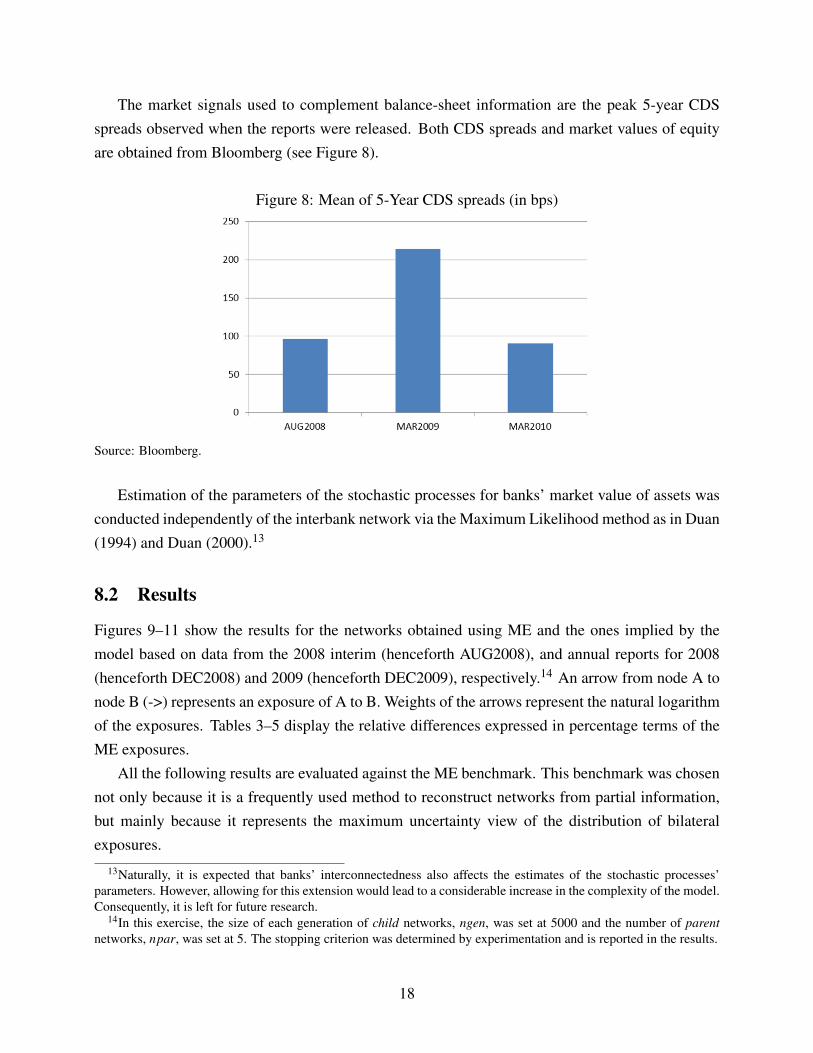
The market signals used to complement balance-sheet information are the peak 5-year CDSspreads observed when the reports were released. Both CDS spreads and market values of equityare obtained from Bloomberg (see Figure 8).
Figure 8: Mean of 5-Year CDS spreads (in bps)
Source: Bloomberg.
Estimation of the parameters of the stochastic processes for banks’ market value of assets wasconducted independently of the interbank network via the Maximum Likelihood method as in Duan(1994) and Duan (2000).13
8.2 Results
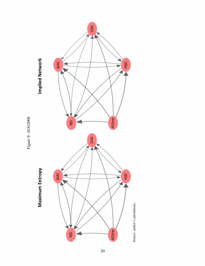
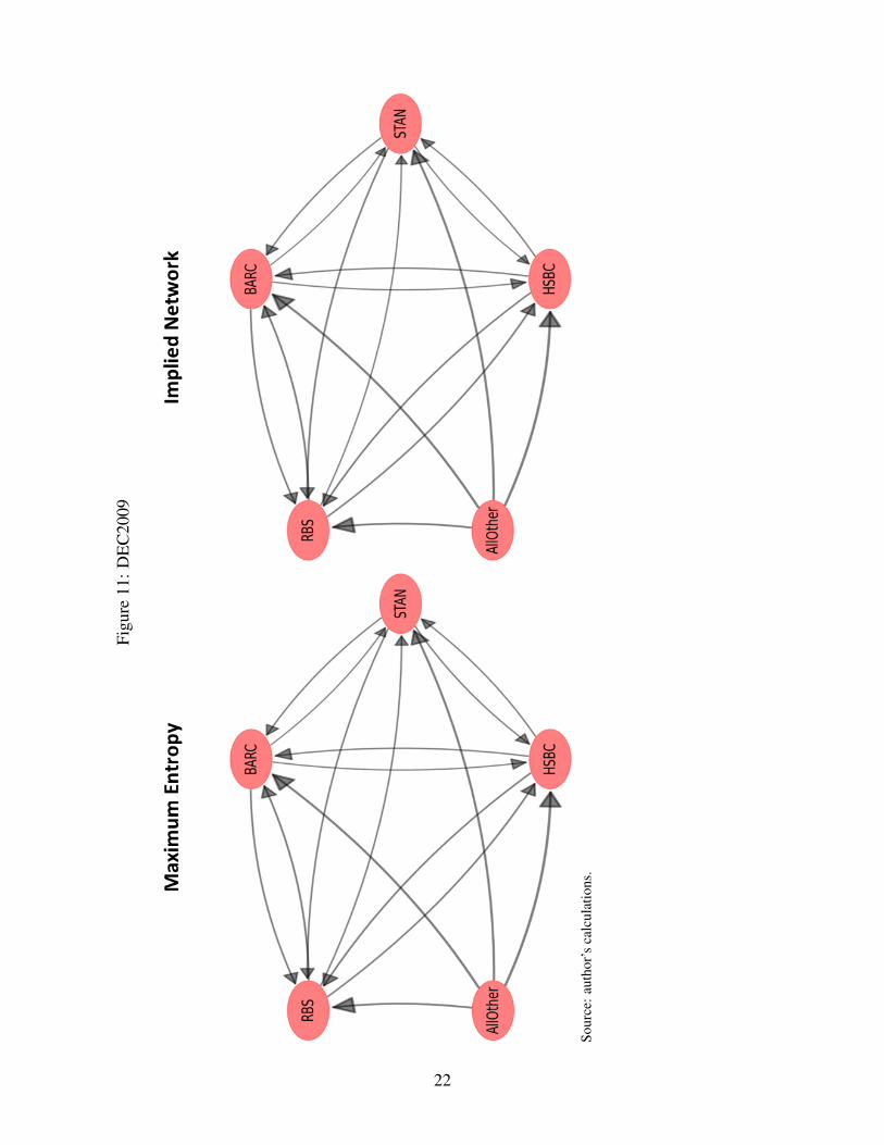
Figures 9–11 show the results for the networks obtained using ME and the ones implied by themodel based on data from the 2008 interim (henceforth AUG2008), and annual reports for 2008(henceforth DEC2008) and 2009 (henceforth DEC2009), respectively.14 An arrow from node A tonode B (->) represents an exposure of A to B. Weights of the arrows represent the natural logarithmof the exposures. Tables 3–5 display the relative differences expressed in percentage terms of theME exposures.
All the following results are evaluated against the ME benchmark. This benchmark was chosennot only because it is a frequently used method to reconstruct networks from partial information,but mainly because it represents the maximum uncertainty view of the distribution of bilateralexposures.
13Naturally, it is expected that banks’ interconnectedness also affects the estimates of the stochastic processes’parameters. However, allowing for this extension would lead to a considerable increase in the complexity of the model.Consequently, it is left for future research.
14In this exercise, the size of each generation of child networks, ngen, was set at 5000 and the number of parentnetworks, npar, was set at 5. The stopping criterion was determined by experimentation and is reported in the results.
18
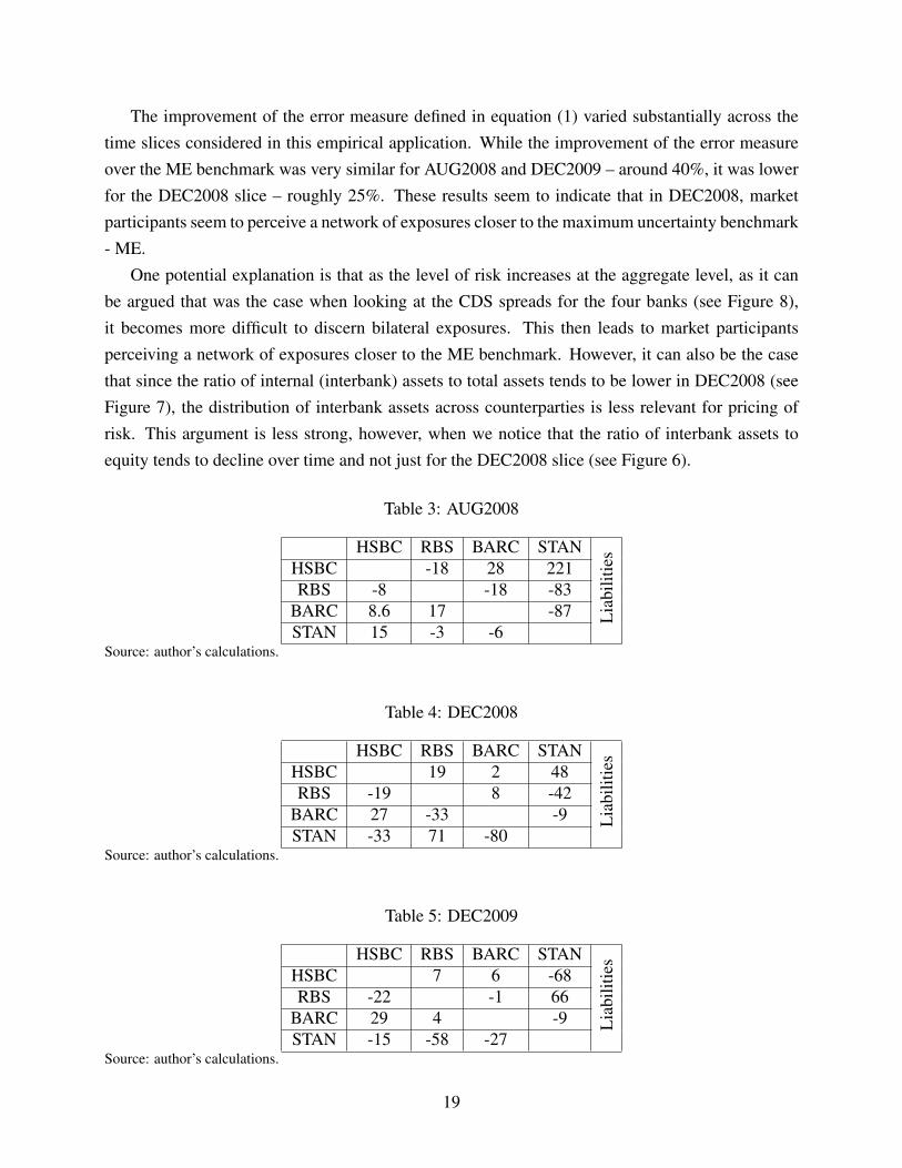
The improvement of the error measure defined in equation (1) varied substantially across thetime slices considered in this empirical application. While the improvement of the error measureover the ME benchmark was very similar for AUG2008 and DEC2009 – around 40%, it was lowerfor the DEC2008 slice – roughly 25%. These results seem to indicate that in DEC2008, marketparticipants seem to perceive a network of exposures closer to the maximum uncertainty benchmark- ME.
One potential explanation is that as the level of risk increases at the aggregate level, as it canbe argued that was the case when looking at the CDS spreads for the four banks (see Figure 8),it becomes more difficult to discern bilateral exposures. This then leads to market participantsperceiving a network of exposures closer to the ME benchmark. However, it can also be the casethat since the ratio of internal (interbank) assets to total assets tends to be lower in DEC2008 (seeFigure 7), the distribution of interbank assets across counterparties is less relevant for pricing ofrisk. This argument is less strong, however, when we notice that the ratio of interbank assets toequity tends to decline over time and not just for the DEC2008 slice (see Figure 6).
Table 3: AUG2008
HSBC RBS BARC STAN
Lia
bilit
ies
HSBC -18 28 221RBS -8 -18 -83
BARC 8.6 17 -87STAN 15 -3 -6
Source: author’s calculations.
Table 4: DEC2008
HSBC RBS BARC STAN
Lia
bilit
ies
HSBC 19 2 48RBS -19 8 -42
BARC 27 -33 -9STAN -33 71 -80
Source: author’s calculations.
Table 5: DEC2009
HSBC RBS BARC STAN
Lia
bilit
ies
HSBC 7 6 -68RBS -22 -1 66
BARC 29 4 -9STAN -15 -58 -27
Source: author’s calculations.
19
Figu
re9:
AU
G20
08
Sour
ce:a
utho
r’s
calc
ulat
ions
.
20

Figu
re10
:DE
C20
08
Sour
ce:a
utho
r’s
calc
ulat
ions
.
21
Figu
re11
:DE
C20
09
Sour
ce:a
utho
r’s
calc
ulat
ions
.
22
9 Conclusion
In this paper, I propose an approach to complement balance-sheet information with market datain order to enhance our understanding regarding the expected relevance of the exposures estab-lished among banks. This approach translates into finding the set of networks that respect the totalamount loaned/borrowed obtained from balance-sheet information and are consistent with marketdata according to a structural valuation model. As an illustration, I present an empirical applica-tion using data for four UK global systemically important banks (G-SIB) referring to the 2007–09financial crisis period. The empirical application to the UK banking system suggests that in timesof stress market participants may find it difficult to discern the network structure of exposures fromthe maximum uncertainty benchmark (i.e., ME).
References
Abbassi, P., C. Brownlees, C. Hans, and N. Podlich (2017). Credit risk interconnectedness: Whatdoes the market really know? Journal of Financial Stability 29, 1 – 12.
Anand, K., B. Craig, and G. Von Peter (2015). Filling in the blanks: Network structure and inter-bank contagion. Quantitative Finance 15(4), 625–636.
Anand, K., I. van Lelyveld, Á. Banai, S. Friedrich, R. Garratt, G. Hałaj, J. Fique, I. Hansen, S. M.Jaramillo, H. Lee, et al. (2017). The missing links: A global study on uncovering financialnetwork structures from partial data. Journal of Financial Stability.
Barucca, P., M. Bardoscia, F. Caccioli, M. D’Errico, G. Visentin, S. Battiston, andG. Caldarelli (2016). Network valuation in financial systems. Available at SSRN:https://ssrn.com/abstract=2795583.
Caballero, R. J. and A. Simsek (2013). Fire sales in a model of complexity. The Journal of
Finance 68(6), 2549–2587.
Chatterjee, S. (2013). Structural credit risk models and systemic capital. Unpublished Manuscript.
Duan, J.-C. (1994). Maximum likelihood estimation using price data of the derivative contract.Mathematical Finance 4(2), 155–167.
Duan, J.-C. (2000). Correction: Maximum likelihood estimation using price data of the derivativecontract (Mathematical Finance 1994, 4/2, 155–167). Mathematical Finance 10(4), 461–462.
23

Egloff, D., M. Leippold, and P. Vanini (2007). A simple model of credit contagion. Journal of
Banking & Finance 31(8), 2475–2492.
Eisenberg, L. and T. H. Noe (2001). Systemic risk in financial systems. Management Science 47(2),236–249.
Elsinger, H., A. Lehar, and M. Summer (2006). Using market information for banking system riskassessment. International Journal of Central Banking 2(1), 137–165.
Fischer, T. (2014). No-arbitrage pricing under systemic risk: Accounting for cross-ownership.Mathematical Finance 24(1), 97–124.
Gandy, A. and L. A. M. Veraart (2016). A Bayesian methodology for systemic risk assessment infinancial networks. Management Science.
Gauthier, C., A. Lehar, and M. Souissi (2012). Macroprudential capital requirements and systemicrisk. Journal of Financial Intermediation 21(4), 594–618.
Gouriéroux, C., J.-C. Heam, and A. Monfort (2013). Liquidation equilibrium with seniority andhidden CDO. Journal of Banking & Finance 37(12), 5261–5274.
House of Commons (2009). Banking Crisis: dealing with the failure of the UK banks.
Hull, J. Options, futures, and other derivatives. New Jersey: Pearson/Prentice Hall, 2009.
Jackwerth, J. C. and M. Rubinstein (1996). Recovering probability distributions from option prices.The Journal of Finance 51(5), 1611–1631.
Langfield, S., Z. Liu, and T. Ota (2014). Mapping the UK interbank system. Journal of Banking &
Finance 45, 288–303.
Li, M., F. Milne, J. Qiu, et al. (2016). Uncertainty in an interconnected financial system, contagion,and market freezes. Journal of Money, Credit and Banking 48(6), 1135–1168.
Merton, R. C. (1974). On the pricing of corporate debt: The risk structure of interest rates. The
Journal of Finance 29(2), 449–470.
Mistrulli, P. E. (2011). Assessing financial contagion in the interbank market: Maximum entropyversus observed interbank lending patterns. Journal of Banking & Finance 35(5), 1114–1127.
Montagna, M. and T. Lux (2017). Contagion risk in the interbank market: A probabilistic approachto cope with incomplete structural information. Quantitative Finance 17(1), 101–120.
24

Pizzuti, C. (2008). Ga-net: A genetic algorithm for community detection in social networks. InInternational Conference on Parallel Problem Solving from Nature. Springer: 1081–1090.
Rogers, L. C. and L. A. Veraart (2013). Failure and rescue in an interbank network. Management
Science 59(4), 882–898.
Schneider, M. H. and S. A. Zenios (1990). A comparative study of algorithms for matrix balancing.Operations Research 38(3), 439–455.
Upper, C. (2011). Simulation methods to assess the danger of contagion in interbank markets.Journal of Financial Stability 7(3), 111–125.
Appendix – Maximum Entropy approach
Consider the following matrix of exposures M, with typical element mi j – the nominal liability offirm i to firm j,
1 2 ... n Liabilities
(li =
n
∑j=1
mi j
)1 0 m12 ... m1n
n
∑j=1
m1 j
2 m21 0 ... m2n
n
∑j=1
m2 j
... ... ... ... ... ...
n mn1 mn2 ... 0n
∑j=1
mn j
Assets
(a j =
n
∑i=1
mi j
)n
∑i=1
mi1
n
∑i=1
mi2 ...n
∑i=1
min
The ME approach approach roughly translates into assuming that banks wish to maximize thedispersion of their interbank assets. Formally, this is achieved by searching for a matrix M that
solves the following cross-entropy problem:
minmi j
n
∑i=1
n
∑j=1
ln
(mi j
m?i j
)s.t. ∑
nj=1 mi j = li, ∑
ni=1 mi j = a j, mi j ≥ 0∀ i 6= j,
25

where m?i j =
a jli ∀ i 6= j
0 otherwise.
This problem can be solved using the RAS algorithm (see Schneider and Zenios 1990).
26