RETURNS ON INVESTMENTS AND VOLATILITY RATE … aefr 3(10)1298-1313.pdf · RETURNS ON INVESTMENTS AND VOLATILITY RATE IN THE ... investment decision requires a forecast of future

Asian Economic and Financial Review, 2013, 3(10):1298-1313

1298

RETURNS ON INVESTMENTS AND VOLATILITY RATE IN THE NIGERIAN

BANKING INDUSTRY

LAWAL A. I.

Department of Accounting and Finance, College of Business and Social Sciences, Landmark University,

Nigeria

OLOYE M. I.

Department of Accounting and Finance, College of Business and Social Sciences, Landmark University, ,

Nigeria

OTEKUNRIN A. O.

Department of Accounting and Finance, College of Business and Social Sciences, Landmark University,,

Nigeria

AJAYI S. A.

Department of Accounting and Finance, College of Business and Social Sciences, Landmark University,

Nigeria

ABSTRACT

Most investment decisions focus on a forecast of future events that is either explicit or implicit.

Generally asset pricing models postulate a positive relationship between a stock portfolio’s

expected returns and risk, which is often modelled by the variance of the asset price. The essence of

this paper is to use GARCH in mean and EGARCH to examine the relationship between mean

returns on the Nigeria commercial banks portfolio investments and its conditional variance or

standard deviation. After estimating a variety of models from Central Bank of Nigeria Statistical

Bulletin 2010 data, we found out that using the GARCH in mean a positive and significant

relationship exist between commercial bank portfolio return and volatility, while the EGARCH

model gives a negative relationship. We suggest that market operators should try as much as

possible to prevent avoidable bad news.

Keywords: Commercial Banks, EGARCH, GARCH-M, Investment, Returns, Volatility

INTRODUCTION

No one invests for fun; every rational investor invests so as to make gain from such an act.

However, the investment climate is characterised with a number of risk limiting investment. Good

Asian Economic and Financial Review

journal homepage: http://aessweb.com/journal-detail.php?id=5002


1299

investment decision requires a forecast of future events that is either explicit or implicit. Since no

one has a perfect picture of the future outcome, as most of the important facts are uncertain, it is

important to reduce the degree of risk and uncertainty associated with such an investment to the

barest minimum before commitment of fund is made. Mainstream theory of finance and investment

teaches that the higher the expected return on an investment the higher the levels of risk or

volatility associate with such an investment. But not all higher risk connote higher return, this

makes intelligent investors to hold portfolio in a manner that will promote higher returns avoiding

higher risk as much as possible. The risk or volatility component of an investment is measured by

the standard deviation and variance of the return of such investment over a period of time. A

number of literature relates returns on an assets to the level of its standard deviation and/or its

variance (see Sharpe (1964), Black. and Scholes (1974), R. (1984). Myung and Jeffrey (2008),

French et al. (1987) Campbell and Hentschel (1993) Sentana (1995), Baillie and Degennaro (1990),

Nelson (1991), Glosten et al. (1993), Rabemananjara and zakoian (1993), Campbell and Hentschel

(1993) ) and Lundblad (2007). Though, these and other authors adopt the use of return variance to

measure risk- volatility, there is no clear consensus view as to what method to use in determining

the relationship between volatility and investment decisions. Also the sample sizes used in

analysing this relationship play crucial roles in determining the nature of results as it was observed

by most of the researchers that small sample always give a negative relationship (see Lundblad

(2007)). However, we have been able to demonstrate that using GARCH in mean, a small sample

size will still give a positive and significant relationship between volatility and return in investment

decisions. The essence of this paper is to examine whether or not volatility affects returns on

investment decisions in the Nigerian banking industry. We humbly submit that we are the first to

use GARCH in mean and EGARCH to examine volatility-return on investment relationship in the

Nigeria banking industry.

This paper is organised as follows: Section 2 provides the literature review; section 3 provides the

methodology used; section 4 presents the empirical results, while section 5 provides conclusion and

recommendations.

LITERATURE REVIEW

Vast literature exist on the casual relationship between volatility and return on financial assets in

the developed economies, for instance Dixit (1995), observed that most business manager are likely

to be neutral towards decision on risk and since investment decisions are rarely repeated, it is

advisable for business decisions to be made solely on the basis of expected return. He explained

that expected return is calculated by weighting each of the profit levels by its associated

probability. For this paper, we examined works relating to the use of GARCH models in measuring

the relationship between returns and volatility on the one hand, and the literatures relating to


1300

commercial banks investment and volatility on the other hand, as hardly could one find existing

literature using GARCH models to directly assess the relationship between banks returns and

volatility.

Garch Models

Developed by Engle (1983) ARCH model was meant to be a model that could assess the validity of

a conjecture of Friedman (1977) that the unpredictability of inflation was a primary cause of

business cycles. The tenet of his hypothesis was that the level of inflation was not a problem; it was

the uncertainty about future costs and prices that would prevent entrepreneurs from investing and

lead to a recession. Today, it has become a household model in measuring volatility and its effects

on a number of economic variables.

Black (1976), Christie (1982), Nelson (1991), Poon and Taylor (1992), using GARCH-M and E-

GARCH models have observed that the asymmetric models are better-off symmetric models as

stock market volatility tends to rise in response to any decrease in stock returns (bad news) and fall

in response to an increase in stock returns (good news). They found out that announcement effect

have a significant leverage effect on the returns of CRSP value weighted stock market index, the

stock returns in UK, Canada, France, Japan and Italy.

Baillie and Degennaro (1990) in a study ‘Stock Returns and Volatility’ examined the econometric

evidence for the relationship between stock returns and stock returns volatility using GARCH in

mean model. Their models show very little evidence for statistically significant relationship

between a stock portfolio’s return and its volatility. Their results suggest traditional two-parameter

models relating portfolio means to variances, which are inappropriate and indicates the need for

research into other measures of risk. They submit that investors consider some other risk measure

to be more important than the variance of portfolio returns (see also Tim Bollerslev (2011)). In

another development, Athanasios et al. (2006) examined the relationship between stock price

returns and volatility for industrialised countries of Australia, Canada, France, Japan, the US, the

UK, Germany and Italy using two models: GARCH-M and E-GARCH and found out that the

GARCH –M model has modelling limitations and gives inconclusive results in comparison with

the E-GARCH model, which provides a more accurate result in respect to the relationship between

stock price return and volatility. They examined the impact of both symmetric and asymmetric (bad

and good news) from stock price on the conditional volatility on the expected returns of these

countries. They found out that the two models show a weak relationship between stock price

returns and volatility for the specific stock market of these industrialized countries (see also De

Santis and A. (2009), Akpan. et al. (2012), Akpan (2012) and Chowdhury et al. (2006). However,

Theodossiou and Lee (1995) examined the relationship between volatility and expected returns

across international stocks markets using alternative version of GARCH-M, and observed that there


1301

is symmetric effect on capital market return across international boarder (see also Berndt and

Hausman (1974), Bollerslev (1987), French et al. (1987), Baillie and Bollerslev (2000) and Engle

et al. (1987). Scholes and Williams (1977) in a paper titled ‘Estimating Betas from

Nonsynchronous Data’ noted that the effect of nonsynchronous data, among other things can be

used to evaluate the level of volatility of data on returns.

Tobias and Joshua (2008) using a cross-sectional pricing of volatility risk to decompose equity

market volatility into short run and long run components found out that prices of risk are negative

and significant for both volatility components. This implies that investors pay for insurance against

increases in volatility even if those increases have little persistence. Their findings suggest that

short run components reveal the market skewness risk or degree of the tightness of financial

constraints, while the long run component is a function of business cycle.

Raggi and Bordignon (2012) in a paper titled ‘Long memory and nonlinearity in realized volatility:

A Markov Switching Approach’ proposed a methodology to analyse the sequential parameter

learning problem for stochastic volatility model with jumps and predictable conditional mean. They

focus on estimating the time invariant parameters and nonobservable dynamics and found out that

simulated and real data is presented to assess the performance of the algorithm. They proposed a

Monte Carlo Algorithm for sequential parameter learning for a stochastic volatility model with

leverage, non constant conditional means and jumps. Their work was an improvement on earlier

authors kernel Smoothing approximation algorithm in which a Monte Carlo Methods MCMC step

is incorporated in order to reduce sampling impoverishment problems.

In another development, Muhammad Imtiaz Subhani et al. (2012) examined the volatility in stock

returns of various stock exchange in relation to interest rates and exchange rates over a range of

eight (8) countries for assorted periods using GARCH (1,1) so as to investigate the possible

eventualities of volatilities of stock markets. They observed that for Pakistan, India, Hong Kong,

Japan, United State, United Kingdom, Spain and Germany various results emerges, though

GARCH (1,1) yielded significant results indicating an existence of volatility of stock markets for

the period under study (i.e 1990-2011). Moreover, there findings suggests that volatility in the

current period is influenced by volatility in the previous lags. Their findings are useful in educating

investors on the trends associated with stock market trends in relating to returns and volatility as

affected by interest rates and / or exchange rate.

Tanij Dutt and Mark (2013) in a paper titled Stock Return Volatility, Operating Performance and

Stock Returns: International Evidence on Drivers of the low Volatility Anomaly examined the links

between stock returns and observed that in line with the existing studies, low volatility stocks earns

higher returns than high volatility stocks in both emerging and developed markets outside the North


1302

America. Their findings also suggests that low volatility stocks have higher operating returns and

this might account for the fact that low volatility attracts higher stock returns. The centre piece of

their work lies in the significant of controlling for stock return volatility when analysing operating

performance and stock performance.

In another development, Dimitrios and Theodore (2011) examined the relationship between

expected stock returns and volatility in the twelve EMU countries as well as five major EMU

international markets between 1992 and 2007 using GARCH in mean models observed that a weak

relationship exist between expected returns and volatility for most of the markets. Their findings

further identified existence of a significant but negative relationship in almost all the markets when

a flexible semi-parametric tools is used for the conditional variance. Moreover, an investigation

was carried out on the asymmetric reaction of volatility to positive and negative shocks in a stock

returns, the result indicates a negative asymmetric in all markets.

Commercial Banks Return-Volatility Relationship

Robert and Karin (1999), used data from 472 commercial banks from 1988 to 1995 to examine

the product mix and earnings volatility of commercial banks in the US and found out that unlike

the conventional wisdom in the banking industry where earnings from fee-based products are more

stable than loan-based earnings, and where fee-based activities reduce bank risk via diversification

a test of the conventional wisdom shows a new ‘degree of total leverage’ framework which

conceptually links a bank’s earnings volatility to fluctuations in its revenues, to the weaken of its

expenses, and to its product mix. They observed various mixes of financial services produced and

marketed jointly within commercial banks, this makes their evidence to reflect the impact of

production synergies (economies of scope) and marketing synergies (cross-selling) not captured in

previous studies. They modify standard degree of leverage estimation methods to conform to the

characteristics of commercial banks. Their results contradicts mainstream believes in that, it was

observed that as the average bank tilts its product mix toward fee-based activities and away from

traditional lending activities, bank’s revenue volatility; its degree of total leverage, and the level of

its earnings all increases. The results of their findings have implications for bank regulators, who

must set capital requirements at levels that balance the volatility of bank earnings against the

probability of bank insolvency. It also suggest another explanation for the shift toward fee-

intensive product mixes: a belief by bank managers that increased earnings volatility will enhance

shareholder value (or at least will increase the value of the managers’ call options on their banks’

stock).

In another development, Kevin (2006), examined the impact of increased non-interest income on

equity market measures of return and risk of U.S. bank holding companies from 1997 to 2004 using

portfolio analytical tools which offers a transparent and informative means for examining the


1303

relative risks and returns of heterogeneous bank activities and find out that non-interest activities

are relatively risky, but yielded similar average returns to shareholders under the year reviewed.

Despite controlling for bank size and equity ratios, which help control for management skills,

internal diversification, leverage, and scale, and for a subset of relatively large banks that one might

expect to be best able to successfully operate in many product markets, the situation still holds. The

implication is that the pervasive shift toward non-interest income has not improved the risk/return

outcomes of U.S. banks in recent years.

Stiroh (2005) explored the link between the growing reliance on non-interest income and the

volatility of bank revenue and profits in the US. He observed that the results from both aggregate

and bank data provide little evidence that shift offers large diversification benefits in the form of

more stable profits or revenue. His findings show that at the aggregate level, noninterest income is

much more volatile than more traditional net interest income. Although net operating revenue has

in fact become less volatile in the 1990s as non-interest income grew in importance, this can be

directly traced to the declining volatility of net interest income that more than offset the increased

contribution from the growing share of the relatively volatile noninterest income. He explained that

trading income, in particular, shows enormous volatility. Moreover, net interest income and

noninterest income growth rates have become more highly correlated in the 1990s.

At the bank level, non-interest income growth also shows an increased correlation with net interest

income over the last decade. Service charges and fees in particular are highly correlated with net

interest income, while trading and fiduciary income is less so. He found negative association

between non-interest income shares and profits per unit of risk for bank risk and return. He

identified trading activities as the biggest drag on profit per unit of risk and suggests that continued

expansion may ultimately lower risk-adjusted returns, while fiduciary income is associated with

higher profit per risk and more stable net income growth. His results questioned the belief that non-

interest income will stabilize revenue and profitability and thereby reduce risk.

In a related development, Kevin and Adrienne (2006) examined the impact of diversification on

risk-return on the US commercial banks to know whether the observed shift toward activities that

generate fees, trading revenue, and other non-interest income has improved the performance of US

Financial Holding Companies (FHCs) from 1997 to 2002, and observed that diversification

benefits exist between FHCs, but these gains are offset by the increased exposure to non-interest

activities, which are much more volatile but not necessarily more profitable than interest-generating

activities. Within FHCs, however, marginal increases in revenue diversification are not associated

with better performance, while marginal increases in non-interest income are still associated with

lower risk-adjusted profits. Their findings revealed that diversification gains are more than offset

by the costs of increased exposure to volatile activities which represents the dark side of the search


1304

for diversification benefits and has implications for supervisors, managers, investors, and

borrowers. Kevin (2006) in a study, ‘New Evidence on the Determinant of Bank Risk’ observed

that two main items: the balance sheet items such as commercial and industrial loans and

consumer lending; and income statement items such as other non-interest income drive the cross-

sectional differences in Bank Holding Company risk. It was stressed that newly mandated

regulatory data on the components of other non-interest income show that investment banking,

servicing, securitization income, gains from loan sales, gains other asset sales, and other non-

interest income are particularly volatile activities. This suggests that the value of increased

transparency as a means to improve market discipline and reduce the difficulty associated with

complex financial institutions. Finally, in the years after 2000, the focus of risk has shifted off the

balance sheet and onto the income statement as investors identify the new risks associated with

evolving and expanding bank activities.

In another development, Dan (2010) in a paper titled ‘Collateral Shortages, Asset Price and

Investment Volatility with Heterogeneous Beliefs’ developed a dynamic general equilibrium model

to examine the effects of belief heterogeneity on the survival of agents and on asset price and

investment volatility under different financial markets structures. He observed that, when financial

markets are endogenously incomplete, agents with incorrect beliefs survive in the long run. The

survival of these agents leads to higher asset price and investment volatility. This is in contrasts

with the frictionless complete markets case, in which agents holding incorrect beliefs are eventually

driven out and as a result, asset prices and investment exhibit lower volatility. His findings show

the existence of stationary Markov equilibrium in the framework with Wealth Distribution and

Asset Price Volatility over Time. The centre piece of his work deals with introduction of a dynamic

general equilibrium model with aggregate shocks potentially incomplete markets and

heterogeneous agents to investigate the role of financial markets. He observed that besides being

risk averse, agents differ in their beliefs about the future aggregate states of the economy. This, he

explained induces them to take large bets under frictionless complete financial markets, which

enable agents to leverage their future wealth. He further explained that under incomplete markets

generated by collateral constraints, agents with heterogeneous (potentially incorrect) beliefs survive

in the long run and their speculative activities drive up asset price volatility and real investment

volatility. He added that collateral constraints are always binding even if the supply of

collateralizable assets endogenously responds to their price. He used this framework to study the

effects of different types of regulations and the distribution of endowments on leverage, asset price

volatility and investment.

It is also important to note that Robert and Karin (1999), established a number of empirical links

between bank non-interest income, business strategies, market conditions, technological change,

and financial performance between 1989 and 2001 so as to determine the nature of return- volatility


1305

level in the US financial market and observed that well-managed banks expand more slowly into

non-interest activities, and that marginal increases in non-interest income are associated with

poorer risk-return tradeoffs on average. They suggested that non-interest income is coexisting with,

rather than replacing, interest income from the intermediation activities that remain banks' core

financial services function.

DATA AND METHODOLOGY

Data

The data used in the study consisted of time series of commercial banks’ investment profile of all

the Nigerian commercial banks sourced from the 2010 Central Bank of Nigeria Statistical Bulletin.

The data spanned from 1992 to 2009

The GARCH in mean specification is as specified as follows:

rt = µ + λht + ϵt , ϵt ~ N (0, ht) (equ. 1)

where rt is the return on investment, u is the risk free return, ht is the conditional variance and λ is

the coefficient that represent the risk-return trade-off.

The EGARCH or the Exponential GARCH model developed by Nelson (1991) provides a good

ground to capture the missing link or inability of GARCH in mean Athanasios et al. (2006) to

provide an even function of the past disturbances, ut-1, ut-2....ut-n . For this work, we used estimates

of the followings augmented version of the E-GARCH model

Rt = βRt-1 + γh2t + ut (equ. 2)

Where Rt is the logarithm investment return at time t

h2t is the conditional heteroskedastic term at time t

ut is the error term

h2t = V (ut/Ωt-1) = E (u

2t/ Ωt-1). However, it is important to note that for h

2t, Nelson (1991)

used an exponential form which is written as:

Log h2

t = α0 +q∑t = lαl(ut-l/ht-l) +

q∑l = 1αl(|ut-l/ht-l|-µ) +

q∑l = 1φllog h

2t-l (equ 3)

where µ=E (|ut/ht|)

As noted by Athanasios et al. (2006), the value of µ depends on the density function assumed for

the standard disturbances, ᶓt = ut/ht, under this condition µ = (2/∏)1/2

,

if ᶓt ≈ Ν ( 0,1).

Also, it should be noted that for unconditional variance to exist, 1-p∑l=1φt ᶓtt = 0 (equ. 4)

The implication is that the root of our equation will fall outside the unit cycle. Furthermore,

Athanasios k. Et al [21] explained that if p∑l = 1 φt ᶓt

t ˂ 1, then the log of unconditional variance

will be given by: log (h2t) = α0(1-p∑l=1φt ᶓtt t)

-1. This makes it clear that the E-GARCH model will

always yield a positive conditional variance.


1306

EMPIRICAL RESULTS

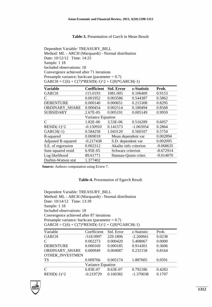
Table 3 below (see appendix) presents the result of our analysis on GARCH in mean model using

Eviews 7, from the table one can deduce that all the variables except Subsidiary shows a positive

relationship when the Treasury bill is the dependent variable. The implication is that, there is

evidence that volatility affects returns. The mean equation at 0.001952 shows that the average

returns is about 1.95%. However, a mixed result is obtained from the volatility coefficients as the

ARCH effects shows a negative effect of -0.150910 while the GARCH effect is at 0.584258. Their

sum is between zero (0) and one (1) i.e. 0.433348, as required by theory (see (William et al.,

2008),Walter (2010)). Furthermore, taking a look at the table, one could see from our GARCH in

mean result that the GARCH- M term 115.0193 is significantly different from zero (0), this shows

that there is evidence that volatility affects returns as there is an established linkages between the

conditional variance and the conditional mean. In other words, as volatility increases, the returns

correspondingly increase by a factor of 115.0193. Our result support Theodossiou and Lee (1995)

findings. This result also supports the usual view in financial market that high risk connotes higher

returns. It should be noted that when bad news hits financial markets, assets prices tends to enter a

turbulent phase and volatility increases, but with positive news, volatility tends to be small and

market enters a period of tranquillity.

The Durbin-Watson stat (1.377402) lies between 0.820 and 1.872; this suggests that there is

inconclusive evidence regarding the presence or absence of positive first order serial correlation

(see Gujarati. and Porter. (2009) Walter (2010) and William et al. (2008)). It should be noted that

measures such as R2 may not be meaningful, if there are no repressor in the mean equation, for

example, the R2 is negative in all the models used. A meaningful value of R

2 will be shown when

diagnostics test is performed on the variables used (see Table 5).

The EGARCH results also shows a mixed result in the Nigeria context as it could be deduced from

Table 4 that the coefficient of the EGARCH terms (-518) is negative which shows that negative

shocks have a larger effects on volatility than positive shocks such that as volatility increase by one

(1), it is accompanied by a fall in return by 518 percent, an indication that the market is highly

volatile and sensitive to announcement effects, this result contradict Athanasios et al. (2006) view

of the supremacy of EGARCH model over GARCH in mean models. Also, it can be deduced from

the table that the mean return on investment (C) is 0.002%. However, the coefficient of the

asymmetric term is negative at -0.22 percent, while that of the GARCH effect is positive at 0.98, a

sum of these two coefficients: 0.75459 is both positive and lies between zero (0) and one (1). The

implication is that the shock on the conditional variance will be highly persistence. This is also in

line with the theory. A large sum of these coefficients connotes that large positive or a large

negative return will lead future forecast of the variance to be high for a protracted period. The


1307

Durbin-Watson stat (1.230350) for the EGARCH also lies between 0.820 and 1.872, which also

suggest that there is inconclusive evidence regarding the presence or absence of positive first order

serial correlation (see Gujarati. and Porter. (2009)).

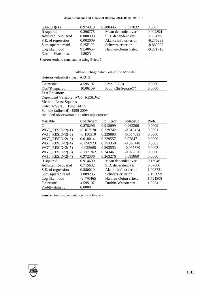
In Table 5, we present the result of diagnostic test, from the table it could be deduced that both the

F-version and LM-statistics are very significant, suggesting the presence of ARCH in the risk-

return relationship (see also (Koenker and Machado, 1999; Guide, 2009). It could be seen from the

table that the lower portion of the outlook shows the goodness of fit measure (pseudo R-squared) to

be about 0.914 meaning that the analysis is about 91.4% explained by the explanatory variables and

the adjusted R is about 0.7156. Though these two results (GARCH-M) and EGARCH shows

different results, one interesting thing about the two results is that it is established from the duo that

volatility affects returns, and that negative shocks have a larger effects on volatility than positive

shocks.

CONCLUSION

This paper examined returns on investments and volatility rate in the Nigerian banking industry for

a period of eighteen years covering 1992 to 2009 using GARCH in mean and EGARCH models

and found out that volatility do affects return on investments made by the banks. We identified the

effects of announcement or news (good or bad) on relationship between risk and returns as both

have a contributory effect on the volatility - return relation on investments decision made by these

banks. We therefore suggest that policy makers and regulators should put in place measures that

will encourage free flow of relevant but good information and avoiding unnecessary bad

information from entering the market. Also bank investment should be tailored towards less

volatile investment so as to reduce the level of volatility witnessed in the market. We recommend

the use of other econometric tools to analyse the nature of risk – return relationship in the market.

REFERENCES

Akpan, S.B., 2012. Analysis of food crop output volatility in agriculture policy

programme regimes in Nigeria. Developing Country Studies, 2(1): 28-35.

Akpan., Udoh. and Umoven., 2012. Modelling the dynamic relationship between food

crop output volatility and its determinants in Nigeria. Journal of Agricultural

Science, 4(8).

Athanasios, K., P. Nicholas and M. Phil, 2006. More evidence on the relationship between

stock price returns and volatility: A note. International Research Journal of

Finance and Economics(1).


1308

Baillie, R. and T. Bollerslev, 2000. The forward premium puzzle is not as bad as you

think. Journal of International Money and Finance, 19: 471-488.

Baillie, R. and R.P. Degennaro, 1990. Stock returns and volatility. The Journal of

Financial and Quantitative Analysis, 25: 203-214.

Berndt, H., Hall., and Hausman, 1974. Estimation and inference in nonlinear structural

models. Annals of Economics and Social Measurement, 3: 653-665.

Black, F., 1976. Studies of stock price volatility changes. pp: 177-181.

Black. and Scholes, 1974.

Bollerslev, T., 1987. A conditionally heteroskedastic time series model for speculative

prices and rates of return. Review of Economics and Statistics, 69: 542-547.

Campbell, J. and L. Hentschel, 1993. No news is good news: An asymmetric model of

changing volatility in stock returns. Journal of Financial Economics, 31: 281-381.

Chowdhury, S.S., Mollik and Akhter, 2006. Does predicted macroeconomic volatility

influence stock market volatility? , Evidence from Bangladesh Capital Market:

Sage Publishers.

Christie, A.A., 1982. The stochastic behavior of common stock variances: Value, leverage

and interest rate effects. Journal of Financial Economics, 10: 407-432.

Dan, C., 2010. Collateral shortages, asset price and investment volatility with

heterogeneous beliefs. Available from www.economics.mit.edu/files4854,

www.richmondfed.org/conferences_and_events/research/2010/pdfcao_paper.pdf.

De Santis, A.R. and F.C. A., 2009. Asset prices, monetary liquidity and business cycle in

an empirical international portfolio allocation model for the united states and the

euro area’. Working papers.

Dimitrios, D. and S. Theodore, 2011. The relationship between stock returns and volatility

in the seven-teen largest international stock markets: A semi-parametric approach.

Modern Economy, 2(1).

Dixit, A., 1995. Irreversible investment with uncertainty and scales economies. Journal of

Economics Dynamics and Control, 19: 327-350.

Engle, R.F., 1983. Estimates of the variance of U.S. Inflation based upon the arch model.

Journal of Money, Credit, and Banking, 15: 286–301.

Engle, R.F., D.M. Lilien and R.P. Robins, 1987. Estimating time varying risk premia in

the term structure: The arch -m model. Econometrica, 55: 391–407.

French, K.R., G.W. Schwert and R.F. Stambaugh, 1987. Expected stock returns and

volatility. Journal of Financial Economics, 19: 3–29.

Friedman, M., 1977. Nobel lecture: Inflation and unemployment. Journal of Political

Economy, 85: 451–472.

http://www.economics.mit.edu/files4854

http://www.richmondfed.org/conferences_and_events/research/2010/pdfcao_paper.pdf


1309

Glosten, L.R., R. Jagannathan and D.E. Runkle, 1993. On the relation between the

expected value and the volatility of the nominal excess return on stocks. Journal

of Finance, 48: 1779–1801.

Guide, E.U.s., 2009. Qms isbn.

Gujarati. and Porter., 2009. Basic econometrics Fifth Edn., McGraw- Hill International.

Kevin, J.S., 2006. New evidence on the determinant of bank risk. Journal of Financial

Services Research, 30(3): 237- 263.

Kevin, J.S. and R. Adrienne, 2006. The dark side of diversification: The case of us

financial holding companies. Journal of Banking & Finance, 30: 2131–2161.

Available from www.elsevier.com/locate/jbf.

Koenker, R., Jose, and A.F. Machado, 1999. Goodness of fit and related inference

processes for quantile regression. Journal of the American Statistical Association,

94(448): 1296-1310.

Lundblad, C., 2007. The risk returns trade of in the long run: 1836-2003. Journal of

Financial Economics, 85: 123-150.

Muhammad Imtiaz Subhani , S.A. Hasan. and Amber Osman, 2012. An application of

garch while investigating volatility in stock returns of the world, posted 15. March

2013 11:32 utc. MPRA Paper No. 45089.

Myung, D.P. and H.D. Jeffrey, 2008. The role of restrictions in estimating the risk-return

trade-off.

Nelson, D., 1991. Conditional heteroskedasticity in asset returns: A new approach.

Econometrica, 59: 347-370.

Poon, S.H. and S.J. Taylor, 1992. Stock returns and volatility: An empirical study of the

U.K. Stock market. Journal of Banking and Finance.

R., P., 1984. Risk, inflation and the stock market. American Economic Review, 74: 335-

351.

Rabemananjara, R. and J.M. zakoian, 1993. Threshold arch models and asymmetries in

volatility. Journal of Applied Econometrics 8: 31-49.

Raggi, D. and S. Bordignon, 2012. Volatility, jumps and predictability of returns: A

sequential analysis. Econometric Reviews, 30(6).

Robert, D. and P.R. Karin, 1999. Product mix and earnings volatility at commercial banks:

Evidence from a degree of leverage model. Working papers series research

department (wp-99-6).

Scholes, M. and J. Williams, 1977. Estimating betas from nonsynchronous data. Journal

of Financial Economics, 5: 307-327.

Sentana, E., 1995. Quadratic arch models. Review of Economic Studies, 62: 639-661.

Sharpe, w., 1964. Capital asset prices: A theory of market equilibrium under conditions of

risk. Journal of Finance, 19: 425–442.

http://www.elsevier.com/locate/jbf


1310

Stiroh, K., J. , 2005. A portfolio view of banking with interest and noninterest assets.

Mimeo: Federal Reserve Bank of New York.

Tanij Dutt and H.-J. Mark, 2013. Stock return volatility, operating performance and stock

returns: International evidence on drivers of the low volatility anomaly. Unsw

Australian school of business research paper no 2012 bfn14. Journal of Banking

and Finance, 37. Available from http//ssrn.com/abstract=2162854 or

http://dx.doi’org/10.2139/ssrn.2162854.

Theodossiou, P. and U. Lee, 1995. Relationship between volatility and expected returns

across international stock markets. Journal of Business Finance and Accounting.

Tim Bollerslev, M.G., Hao Zhou,, 2011. Dynamic estimation of volatility risk premia and

investor risk aversion from option-implied and realized volatilities. Journal of

Econometrics, 160.

Tobias, A. and Joshua, 2008. Stock returns and volatility: Pricing the short run and long

run components of market risk. The Journal of Finance, LXIII(6).

Walter, E., 2010. Applied econometric time series. 3rd Edn.: John Wiley & Sons.

William, E.G., H. Carter, R. and C.L. Guay, 2008. Principle of econometrics. 3rd Edn.:

John Wiley & Sons.

APPENDIX:

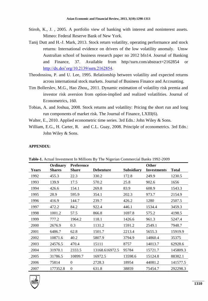
Table-1. Actual Investment In Millions By The Nigerian Commercial Banks 1992-2009

Years

Ordinary

Shares

Preference

Share Debenture Subsidiary

Other

Investments Total

1992 455.3 22.3 330.2 172.8 249.9 1230.5

1993 139.9 17.5 570.2 25.8 902.6 1656

1994 426.6 154.1 269.8 83.9 608.9 1543.3

1995 28.9 595.9 354.1 202.3 973.7 2154.9

1996 416.9 144.7 239.7 426.2 1280 2507.5

1997 472.2 84.2 922.4 446.1 1534.4 3459.3

1998 1001.2 57.5 866.8 1697.8 575.2 4198.5

1999 777.2 1964.2 118.1 1426.6 961.3 5247.4

2000 2676.9 0.3 1131.2 1591.2 2549.1 7948.7

2001 6486.7 62.8 1501.7 2213.4 5655.3 15919.9

2002 10871.6 40.2 5807.9 3794.9 14860.4 35375

2003 24576.5 470.4 15111 8757 14013.7 62928.6

2004 31970.1 2333.5 13168.616972.5 95784 15721.7 145809.3

2005 31786.5 10899.7 16972.5 13598.6 15124.8 88382.1

2006 75814 0 2728.3 18954 44081.2 141577.5

2007 177352.8 0 631.8 38859 75454.7 292298.3

http://dx.doi’org/10.2139/ssrn.2162854


1311

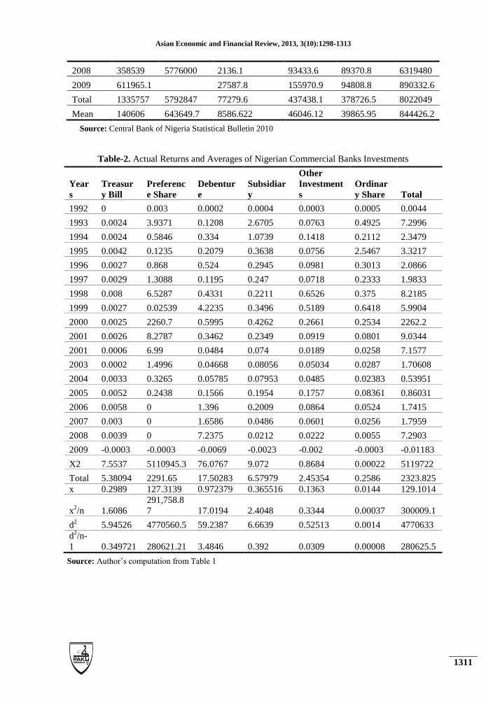
2008 358539 5776000 2136.1 93433.6 89370.8 6319480

2009 611965.1

27587.8 155970.9 94808.8 890332.6

Total 1335757 5792847 77279.6 437438.1 378726.5 8022049

Mean 140606 643649.7 8586.622 46046.12 39865.95 844426.2

Source: Central Bank of Nigeria Statistical Bulletin 2010

Table-2. Actual Returns and Averages of Nigerian Commercial Banks Investments

Year

s

Treasur

y Bill

Preferenc

e Share

Debentur

e

Subsidiar

y

Other

Investment

s

Ordinar

y Share Total

1992 0 0.003 0.0002 0.0004 0.0003 0.0005 0.0044

1993 0.0024 3.9371 0.1208 2.6705 0.0763 0.4925 7.2996

1994 0.0024 0.5846 0.334 1.0739 0.1418 0.2112 2.3479

1995 0.0042 0.1235 0.2079 0.3638 0.0756 2.5467 3.3217

1996 0.0027 0.868 0.524 0.2945 0.0981 0.3013 2.0866

1997 0.0029 1.3088 0.1195 0.247 0.0718 0.2333 1.9833

1998 0.008 6.5287 0.4331 0.2211 0.6526 0.375 8.2185

1999 0.0027 0.02539 4.2235 0.3496 0.5189 0.6418 5.9904

2000 0.0025 2260.7 0.5995 0.4262 0.2661 0.2534 2262.2

2001 0.0026 8.2787 0.3462 0.2349 0.0919 0.0801 9.0344

2001 0.0006 6.99 0.0484 0.074 0.0189 0.0258 7.1577

2003 0.0002 1.4996 0.04668 0.08056 0.05034 0.0287 1.70608

2004 0.0033 0.3265 0.05785 0.07953 0.0485 0.02383 0.53951

2005 0.0052 0.2438 0.1566 0.1954 0.1757 0.08361 0.86031

2006 0.0058 0 1.396 0.2009 0.0864 0.0524 1.7415

2007 0.003 0 1.6586 0.0486 0.0601 0.0256 1.7959

2008 0.0039 0 7.2375 0.0212 0.0222 0.0055 7.2903

2009 -0.0003 -0.0003 -0.0069 -0.0023 -0.002 -0.0003 -0.01183

X2 7.5537 5110945.3 76.0767 9.072 0.8684 0.00022 5119722

Total 5.38094 2291.65 17.50283 6.57979 2.45354 0.2586 2323.825

x 0.2989 127.3139 0.972379 0.365516 0.1363 0.0144 129.1014

x2/n 1.6086

291,758.8

7 17.0194 2.4048 0.3344 0.00037 300009.1

d2 5.94526 4770560.5 59.2387 6.6639 0.52513 0.0014 4770633

d2/n-

1 0.349721 280621.21 3.4846 0.392 0.0309 0.00008 280625.5

Source: Author’s computation from Table 1


1312

Table-3. Presentation of Garch in Mean Result

Dependent Variable: TREASURY_BILL

Method: ML - ARCH (Marquardt) - Normal distribution

Date: 10/12/12 Time: 14:25

Sample: 1 18

Included observations: 18

Convergence achieved after 71 iterations

Presample variance: backcast (parameter = 0.7)

GARCH = C(6) + C(7)*RESID(-1)^2 + C(8)*GARCH(-1)

Variable Coefficient Std. Error z-Statistic Prob.

GARCH 115.0193 1081.005 0.106400 0.9153

C 0.001952 0.003586 0.544387 0.5862

DEBENTURE 0.000140 0.000651 0.215308 0.8295

ORDINARY_SHARE 0.000454 0.002514 0.180494 0.8568

SUBSIDARY 2.67E-05 0.005191 0.005149 0.9959

Variance Equation

C 1.82E-06 3.53E-06 0.516289 0.6057

RESID(-1)^2 -0.150910 0.141573 -1.065954 0.2864

GARCH(-1) 0.584258 1.043120 0.560107 0.5754

R-squared 0.069018 Mean dependent var 0.002894

Adjusted R-squared -0.217438 S.D. dependent var 0.002095

S.E. of regression 0.002312 Akaike info criterion -9.068635

Sum squared resid 6.95E-05 Schwarz criterion -8.672914

Log likelihood 89.61771 Hannan-Quinn criter. -9.014070

Durbin-Watson stat 1.377402

Source: Authors computation using Eview 7.

Table-4. Presentation of Egarch Result

Dependent Variable: TREASURY_BILL

Method: ML - ARCH (Marquardt) - Normal distribution

Date: 10/14/12 Time: 13:39

Sample: 1 18

Included observations: 18

Convergence achieved after 87 iterations

Presample variance: backcast (parameter = 0.7)

GARCH = C(6) + C(7)*RESID(-1)^2 + C(8)*GARCH(-1)

Variable Coefficient Std. Error z-Statistic Prob.

GARCH -518.0997 229.1806 -2.260661 0.0238

C 0.002273 0.000420 5.408067 0.0000

DEBENTURE 0.000169 0.000185 0.914301 0.3606

ORDINARY_SHARE 0.000949 0.004087 0.232158 0.8164

OTHER_INVESTMEN

TS 0.009766 0.005174 1.887605 0.0591

Variance Equation

C 6.83E-07 8.63E-07 0.792186 0.4283

RESID(-1)^2 -0.219729 0.160382 -1.370038 0.1707


1313

GARCH(-1) 0.974319 0.288445 3.377832 0.0007


Adjusted R-squared 0.080398 S.D. dependent var 0.002095

S.E. of regression 0.002009 Akaike info criterion -9.276283

Sum squared resid 5.25E-05 Schwarz criterion -8.880562

Log likelihood 91.48654 Hannan-Quinn criter. -9.221718

Durbin-Watson stat 1.8923

Source: Authors computation using Eview 7.

Table-5. Diagnostic Test of the Models

Heteroskedasticity Test: ARCH

F-statistic 4.595107 Prob. F(7,3) 0.0000

Obs*R-squared 10.06159 Prob. Chi-Square(7) 0.0000

Test Equation:

Dependent Variable: WGT_RESID^2

Method: Least Squares

Date: 02/22/13 Time: 14:55

Sample (adjusted): 1999 2009

Included observations: 11 after adjustments

Variable Coefficient Std. Error t-Statistic Prob.

C 0.878296 0.912699 0.962306 0.0009

WGT_RESID^2(-1) -0.187570 0.229742 -0.816434 0.0001

WGT_RESID^2(-2) -0.150510 0.229893 -0.654695 0.0000

WGT_RESID^2(-3) 0.018014 0.229557 0.078471 0.0000

WGT_RESID^2(-4) -0.098923 0.253358 -0.390448 0.0003

WGT_RESID^2(-5) -0.025665 0.263553 -0.097380 0.0003

WGT_RESID^2(-6) -0.005362 0.243461 -0.022026 0.0000

WGT_RESID^2(-7) 0.972506 0.263276 3.693860 0.0000


Adjusted R-squared 0.715632 S.D. dependent var 0.87666

S.E. of regression 0.580010 Akaike info criterion 1.903721

Sum squared resid 1.009236 Schwarz criterion 2.193099

Log likelihood -2.470465 Hannan-Quinn criter. 1.721308

F-statistic 4.595107 Durbin-Watson stat 1.9854

Prob(F-statistic) 0.0000

Source: Authors computation using Eveiw 7

Documents

RETURNS ON INVESTMENTS AND VOLATILITY RATE … aefr 3(10)1298-1313.pdf · RETURNS ON INVESTMENTS AND VOLATILITY RATE IN THE ... investment decision requires a forecast of future