1

RETURNS TO CAPITAL IN MICROENTERPRISES: EVIDENCE FROM A FIELD EXPERIMENT♣

Suresh de Mel David McKenzie

and Christopher Woodruff

Abstract We use randomized grants to generate shocks to capital stock for a set of Sri Lankan microenterprises. We find the average real return to capital in these enterprises is 4.6-5.3 percent per month (55-63 percent per year), substantially higher than market interest rates. We then examine the heterogeneity of treatment effects. Returns are found to vary with entrepreneurial ability and with household wealth, but not to vary with measures of risk aversion or uncertainty. Treatment impacts are also significantly larger for enterprises owned by males; indeed, we find no positive return in enterprises owned by females.

♣ The authors thank David I. Levine for early discussions on this project, and Shawn Cole, Xavier Gine, Gordon Hanson, Larry Katz, Craig McIntosh, Jonathan Morduch, Edward Vytlacil, Bilal Zia, three anonymous referees and participants at various seminars for comments. Susantha Kumara, Jose Martinez and Jayantha Wickramasiri provided outstanding research assistance. AC Nielsen Lanka administered the surveys on which the data are based. Financial support from NSF grant # SES-0523167 and the World Bank is gratefully acknowledged. This paper was drafted in part while Woodruff was visiting LSE, whose support is also gratefully acknowledged.

2

1. Introduction

Small and informal firms are the source of employment for half or more of the

labor force in most developing countries. A central question for policymakers is whether

these firms hold the potential for income growth for their owners, or whether they merely

represent a source of subsistence income for low-productivity individuals unable to find

alternative work. The rapid increase in development funding being channeled to

microfinance organizations is based on belief that these firms can earn high returns to

capital if given the opportunity. Evidence that some firms have high marginal returns is

suggested by the very high interest rates paid to moneylenders, and by literature which

identifies the effect of credit shocks on those who apply for credit (see Banerjee and

Duflo (2005) for an excellent recent summary). However, the sample of firms who apply

for credit or who belong to microfinance organizations does not represent the full

universe of firms for a number of reasons.1 We lack a credible estimate of returns among

firms not borrowing from formal sources.

In this paper we use a randomized experiment to identify the effect of incremental

cash investments on the profitability of all enterprises, irrespective of whether or not they

choose to apply for credit at market interest rates. We then examine the heterogeneity of

returns in order to test which theories can explain why firms may have marginal returns

well above the market interest rate. We accomplish this by surveying microenterprises in

Sri Lanka and providing small grants to a randomly selected subset of the sampled firms.

We purposely restricted our survey to firms with less than 100,000 Sri Lankan rupees

(LKR, about $1000) in capital other than land and buildings. The grants were either

10,000 LKR (about $100), or 20,000 LKR (about $200). The larger grants were equal to

more than 100 percent of the 18,000 LKR baseline median level of invested capital.

1 These reasons include both selection among entrepreneurs as to whether or not to apply for credit, determined by factors such as their attitudes to risk, access to alternative sources of finance, perceptions of the returns on investment, and expectations of getting a loan; as well as selection on the part of the lender as to which firms to accept as clients. Microfinance lending methodologies like group lending may also cause some potential borrowers to forgo loans (Gine and Karlan, 2007.)

3

An accurate measurement of returns to capital is critical to understanding the

potential of microfinance. With more than 70 million clients worldwide, microfinance

NGOs are now the most common source of credit for household enterprises, and one of

the largest channels for development aid. But available evidence on take-up rates

suggests that only a small percentage of those informed about microfinance programs

desire loans. Is the return to capital lower than interest rates for non-borrowers? Or do

other factors—risk aversion or low levels of financial literacy, for example—prevent

potentially beneficial loans from being requested? In spite of the rapid spread of

microfinance in recent years, there is surprisingly little evidence of its effectiveness in

raising incomes of borrowers. Reviewing the literature, Armendáriz de Aghion and

Morduch (2005) conclude: “The number of careful impact studies is small but growing,

and their conclusions, so far, are [measured].” The small number of studies owes in part

to the difficulty of identifying a comparison sample (Karlan 2001; Morduch 1999). We

generate an identical comparison among firms in our sample through randomization.

Measuring returns at low levels of capital stock also provides important feedback

to theory. The theoretical literature on occupational choice has posited a minimum scale

below which returns to capital are very low or even zero.2 Low returns at low levels of

capital stock would suggest that individuals without access to a sufficient amount of

capital would face a permanent disadvantage. That is, they would fall into a poverty trap.

If, on the other hand, returns are high at low levels of capital stock, then entrepreneurs

entering with sub-optimal capital stocks would be able to grow by reinvesting profits. In

this case, entrepreneurs might remain inefficiently small for some period of time, but

would not be permanently disadvantaged. In the absence of minimum scale, we might

2 Banerjee and Newman (1993) and Aghion and Bolton (1997) are seminal papers in this literature. Because we study a sample of enterprises that existed at the time of the baseline survey, we can only provide evidence on the importance of non-convexities conditional on entry. The loss of income resulting from starting an unsuccessful business might be an additional barrier to entry for low-wealth households.

4

expect returns to be high. Because small scale entrepreneurs lack access to credit at

market interest rates, risk-adjusted returns may well be higher than market interest rates.

There is an increasing number of estimates of returns to capital in small scale

productive activities in developing countries (see Banerjee and Duflo 2005). Some of the

estimates come from broad cross-sections of producers, and others from the subset of

firms exposed to some shock. Among the former, McKenzie and Woodruff (2006)

estimate returns to capital among the smallest urban microenterprises in Mexico, those

with less than $US200 invested, of around 15 percent per month, or an uncompounded

rate of 180 percent per year. Returns in the Mexican data fall to around 40-60 percent per

year above $500 of capital stock. McKenzie and Woodruff (2008) undertake an

experiment similar to that reported on here among a small sample of enterprises in

Mexico with less than $900 of capital stock. They find returns in the range of 250-360

percent per year, higher than the cross-sectional estimates in their earlier work. Udry and

Anagol (2006) estimate returns in a sample of small scale agricultural producers in Ghana

to be 50 percent per year among those producing traditional crops on a median-sized plot

and 250 percent per year among those producing non-traditional crops on median sized

plots. Banerjee and Duflo (2004) take advantage of changes in the criteria identifying

firms eligible for earmarked credit from Indian banks. The changes in the laws result in

credit supply shocks to identifiable sets of firms, allowing for the identification of the

impact of changes in access to finance among this subset of firms. Banerjee and Duflo

derive estimates of returns for this set of firms of between 74 and 100 percent per year.

The central challenge in estimating returns to capital is that the optimal level of

capital stock is likely to depend on attributes of entrepreneurial ability which are difficult

to measure. Banerjee and Duflo point to one way around this problem—exploiting an

exogenous shock which is uncorrelated with entrepreneurial ability. But this approach has

a downside, in that the sample is limited to firms or entrepreneurs exposed to the shock.

In the case of Banerjee and Duflo’s estimates, the estimates apply only to those firms

5

applying for credit. This resolves one problem at the cost of creating another: While

estimated returns are less subject to ability bias, self-selection of the subsample suggests

the returns likely overstate those for the full spectrum of firms. But low returns to capital

are only one of several possible reasons entrepreneurs may fail to apply for loans. Firms

may lack information about lenders, or overestimate the probability they will be denied a

loan. Estimating returns of firms not applying for formal credit is a first step to

developing policies to address the constraints faced by small firms.

The difficulty of obtaining an unbiased estimate of returns to capital for all

microenterprises, regardless of whether or not they are active borrowers, is the motivation

for the field experiment on which the data used in this paper are based. We use random

grants of either cash or equipment to generate changes in capital against which changes in

profits can be measured. Randomized experiments have quickly become an important

part of the toolkit of development economics (Duflo, Glennerster and Kremer 2006),

although this is the first experiment we are aware of involving payments to firms, rather

than households or schools. The random allocation of the grants ensures that the changes

in capital stock are uncorrelated with entrepreneurial ability, demand shocks, and other

factors associated with the differences in the profitability of investments across firms.

We first use the data to measure the effect of assignment to each of four

treatments on capital stock, profits, and hours worked by the owner. After establishing

that the treatments did have the expected positive effect on capital stock and profits, we

examine the reasonableness of pooling both the four treatments and the data from the

various waves of the survey. We then describe the conditions under which we can use the

random treatments as instruments for capital stock, and estimate the real marginal return

on capital using IV regressions.

We find that both the treatment effects and, for reasonable values of the owner’s

labor time, the returns to capital, range from 4.6 to 5.3 percent per month, on the order of

60 percent per year. We find that there is considerable heterogeneity of the returns along

6

measurable dimensions. We set out a model consistent with our data which can be used to

investigate the importance of imperfect credit markets and imperfect insurance markets.

The model predicts that with imperfect finance and insurance markets, returns to the

shocks to capital stock should be higher for more constrained entrepreneurs, and those

who are more risk averse and face greater uncertainties in sales and profits. Examination

of the heterogeneity of treatment effects shows that returns to capital are generally higher

for entrepreneurs who are more severely capital constrained—those with higher ability

and with fewer other wage workers in the household that can provide liquidity. One

important exception to this is that while the conventional wisdom holds that women are

more severely credit constrained, we find the returns are much higher in enterprises

owned by males than in enterprises owned by females. We do not find that the treatment

effects vary significantly with measures of risk aversion or uncertainty. Taken at face

value, the heterogeneity of returns suggest that the high returns are more closely

associated with missing credit markets than missing insurance markets.

We show that the results are robust to accounting for spillovers on firms located

near the treated firms, to attrition from the sample, and to measurement issues. Finally,

we use both the baseline data and the untreated panel to compare returns generated by

OLS, random- and fixed effects regressions with those generated by the experiment. We

find that the experimental returns are more than twice as large as the non-experimental

returns. Attenuation bias arising from the imprecise measurement of capital stock appears

to be the most plausible reason for the underestimate of the non-experimental returns.

2. Description of Experiment

We carried out a baseline survey of microenterprises in April 2005 as the first

wave of the Sri Lanka Microenterprise Survey (SLMS).3 Eight additional waves of the

3 Fieldwork was carried out by ACNielsen Lanka (Pvt) Ltd.

7

panel survey were then conducted at quarterly intervals, through April 2007. The survey

took place in three Southern and South-Western districts of Sri Lanka: Kalutara, Galle

and Matara. The survey is designed to also study the process of recovery of

microenterprises from the December 26, 2004 Indian Ocean tsunami, and so these

districts were selected as ones where coastal areas had received tsunami damage. The

sample was drawn equally from areas along the coast where firms suffered direct damage

from the tsunami; areas slightly inland where firms did not suffer direct damage, but

where demand may have been affected; and inland areas where neither assets nor demand

are likely to have been affected by the tsunami. We refer to these areas as directly

affected, indirectly affected, and unaffected zones. We set out to draw a sample of firms

with invested capital of 100,000 LKR (about US$1000) or less, excluding investments in

land and buildings. This size cut-off was chosen in order that our treatments (described

below) would be a large shock to business capital.

We began by using the 2001 Sri Lankan Census to select 25 Grama Niladhari

divisions (GNs) in these three districts. A GN is an administrative unit containing on

average around 400 households. We used the Census to select GNs with a high

percentage of own-account workers and modest education levels, since these were most

likely to yield enterprises with invested capital below the threshold we had set.4 The GNs

were stratified according to whether the area was directly affected, indirectly affected, or

unaffected by the tsunami. A door-to-door screening survey was then carried out among

households in each of the selected GNs. This survey was given to 3361 households, with

fewer than 1 percent of households refusing to be listed. The screening survey identified

self employed workers outside of agriculture, transportation, fishing, and professional

services who were between the ages of 20 and 65 and had no paid employees.

4 Although we avoided GNs with high average education levels, the median education level in our sample (10 years) is the same as the median level in the Sri Lankan labor force survey for all adults aged 20-65 years. The mean level is only slightly lower (8.9 vs. 9.4 years). We believe the resulting sample is representative of a substantial majority of the own account workers in Sri Lanka.

8

The full survey was given to 659 enterprises meeting these criteria. After

reviewing the baseline survey data, we eliminated 41 enterprises either because they

exceeded the 100,000 LKR maximum size or because a follow-up visit could not verify

the existence of an enterprise. The remaining 618 firms constitute the baseline sample.

We present results later in the paper indicating that returns to capital were higher among

firms directly affected by the tsunami, but we exclude these firms for most of the analysis

because the tsunami-recovery process might affect returns to capital. We leave the full

analysis of the impact of the capital shocks on enterprise recovery to another paper.

Excluding the directly affected firms leaves us with a baseline sample of 408 enterprises.

The 408 firms are almost evenly split across two broad industry categories, with

203 firms in retail sales and 205 in manufacturing/services. Firms in retail sales are

typically small grocery stores. The manufacturing/services firms cover a range of

common occupations of microenterprises in Sri Lanka, including sewing clothing,

making lace products, making bamboo products, repairing bicycles, and making food

products such as hoppers and string hoppers.

The Experiment

The aim of our experiment was to provide randomly selected firms with a positive

shock to their capital stock, and to measure the impact of the additional capital on

business profits. Firms were told before the initial survey that we would survey them

quarterly for five periods, and that after the first wave of the survey, we would conduct a

random prize drawing, with prizes of equipment for the business or cash. The random

drawing was framed as compensation for participating in the survey. We indicated to the

owners that they would receive at most one grant. For logistical reasons, we distributed

just over half the prizes awarded after the first wave of the survey, and the remaining

prizes after the third wave, with enterprises not given a prize after the first wave not told

whether or not they had won one of the prizes to be awarded in the second distribution

9

until after the third wave. The prize consisted of one of four grants: 10,000 LKR (~$100)

of equipment or inventories for their business, 20,000 LKR in equipment/inventories,

10,000 LKR in cash, or 20,000 LKR in cash. In the case of the in-kind grants, the

equipment was selected by the enterprise owner, and purchased by our research

assistants.5 Subsequently, we received funding to extend the panel to nine waves. As this

represented an extension of the survey relative to what firms were told before the baseline

survey, we granted each of the untreated firms 2,500 LKR (~ $25) after the fifth wave.

The randomization was stratified within district (Kalutara, Galle, and Matara) and

zone (unaffected and indirectly affected by the tsunami). Allocation to treatment was

done ex ante among the 408 firms kept in the sample after the baseline survey.6 A total of

124 firms receive a treatment after round 1, with 84 receiving a 10,000 LKR treatment

and 40 receiving a 20,000 LKR treatment. Another 104 firms were selected at random to

receive a treatment after the third survey round: 62 receiving the 10,000 LKR treatment

and 42 the 20,000 LKR treatment. In each case half the firms receiving a treatment

amount received cash, and the other half equipment.

The 10,000 LKR treatment is equivalent to about three months of median profits

reported by the firms in the baseline survey, and the larger treatment equivalent to six

months of median profits. The median initial level of invested capital, excluding land and

buildings, was about 18,000 LKR, implying the small and large treatments correspond to

approximately 55 percent and 110 percent of the median initial invested capital. By either

measure, the treatment amounts were large relative to the size of the firms.

5 In order to purchase the equipment for these entrepreneurs receiving equipment treatments, research assistants visited several firms in the evening to inform them they had won an equipment prize. The winning entrepreneurs were asked what they wanted to buy with the money, and where they would purchase it. The research assistants then arranged to meet them at the market where the goods were to be purchased at a specified time the next day. Thus, the goods purchased and the place/market where they were purchased were chosen by the entrepreneurs with no input from the research assistants. 6 The authors carried out the randomization privately by computer. The ex-ante treatment allocation was kept private from both the survey firm and the firms participating in the survey, with firms only learning they had received a treatment at the time it was given out. Seven firms assigned to receive a treatment after round 3 attrited between the second and third rounds.

10

Although the amount offered for the in-kind treatment was either 10,000 LKR or

20,000 LKR, in practice the amount spent on inventories and equipment sometimes

differed from this amount. Among those receiving equipment, only four of the 116 firms

receiving equipment treatments spent as much as 50 LKR ($0.50) less than the amount

we offered. More commonly, the entrepreneurs contributed funds of their own to

purchase a larger item. This occurred in 65 of the 116 equipment treatments. However, in

44 of the 65 cases, the owners contributed less than 500 LKR, or $5. The entrepreneurs

contributed 2000 rupees or more in only 13 percent of the cases. We use the amount

offered rather than the amount spent in our analysis of the effects of treatment. We have

both receipts and pictures of the goods purchased with the equipment grants.

Approximately 57 percent of the purchases were inventories or raw materials, 39 percent

machinery or equipment, and 4 percent construction materials for buildings.

Cash treatments were given without restrictions. Those receiving cash were told

that they could purchase anything they wanted, whether for their business or for other

purposes. In reality, the grant was destined to be unrestricted because we lacked the

ability to monitor what recipients did with the funds, and because cash is fungible. Being

explicit about this was intended to produce more honest reporting regarding use of the

funds. In the survey subsequent to the treatment, we asked how they had used the

treatment.7 On average, 58 percent of the cash treatments was invested in the business

between the time of the treatment and the subsequent survey. An additional 12 percent

was saved, 6 percent was used to repay loans, 5 percent spent on household consumption,

4 percent on repairs to the house, 3 percent on equipment or inventories for another

business, and the remaining 12 percent spent on “other items.” Of the amount invested in

the enterprise, about two-thirds was invested in inventories and the rest in equipment.

7 Our question noted that some entrepreneurs had told us they had spent the money on furniture or other items for the household, some had spent it on food and clothing, and some had invested in their business. In fact, they had told us this during piloting of the round 2 survey.

11

Both the cash and equipment treatments invested in the firm were almost

exclusively spent on expanding the existing line of business, purchasing similar types of

inventories and equipment as firms would do with reinvestments of retained earnings.

Only three of the treated firms reported changing their line of business after treatment,

and these were changes to different products within retail sales. Treated firms were also

not more likely to introduce new products: 18.9 percent of treated firms introduced a new

product during the year following the baseline survey, compared to 15.6 percent of never

treated firms (p=.40). It is not thus the case that the treatments were being used to fund

particularly risky new endeavors.8

3. Data and Measurement of Main Variables

The baseline survey gathered detailed information on the firm and the

characteristics of the firm owner. The main outcome variable of interest in this paper is

the profits of the firm. Firm profits were elicited directly from the firm by asking: “What was the total income the business earned during March after paying all expenses including wages of employees, but not including any income you paid yourself. That is, what were the profits of your business during March?”

The reported mean and median profits in the baseline are 3850 rupees and 3000

rupees respectively. The survey also asked detailed questions on revenues and expenses.

Profits calculated as reported revenues minus reported expenses are lower, around 2500

at the mean and 1350 at the median. Profits calculated in this manner are positively

correlated with reported profits, with a correlation coefficient of .32. This is about the

same level as one finds in other microenterprise surveys. In de Mel, McKenzie and

Woodruff (2008a), we analyze the measurement of profits in detail, reporting on

experiments conducted with different questions, bookkeeping, and monitoring of sales. 8 Furthermore, we find no relationship between the share of the cash treatment invested in the business and the risk aversion of the owner, which is consistent with the view that the treatments are not being used for particularly risky investments.

12

The biggest reason reported and calculated profits differ is a mismatch of the timing of

purchases and the sales associated with those purchases. Some of the expenses in one

month are associated with sales the following month. Correcting for this mistiming

increases the correlation with reported profits to around .70. We conclude from the more

detailed analysis of measurement issues that the reported profit is the best measure of the

firm’s profitability, and we use those data for the remainder of this paper. In the online

appendix, we show that the effects we find are robust to other outcome measures.

The baseline survey also gathered detailed information on the replacement cost of

assets used in the enterprise, and whether they were owned or rented. Almost all (99

percent) assets excluding land and buildings are owned by the enterprises. The majority

of assets owned by the enterprises are land and buildings. In the baseline sample, these

average 121,000 LKR ($1200), though about a sixth (15 percent) of firms report they

own no assets in this category. The firms also reported an average of 14,400 LKR ($145)

rupees worth of machinery and equipment and 13,000 LKR ($130) in inventories.

In each subsequent round of the survey, we asked firms to report on the purchase

of new assets, the disposition of assets by sale or damage, and the repair and return to

service of any previously damaged assets. Changes in the market value of fixed assets are

calculated from the responses to these questions. Combined with the data from each

previous quarter, these data allow us to estimate equipment investment levels for each

quarter of the survey.9 The survey also asks the current value of inventories of raw

material, work in progress and final goods each quarter. The specific questions related to

the measurement of capital stock are described in the online appendix.

Of the 408 firms in the baseline survey, 369 completed the ninth wave, an attrition

rate of only 9.6 percent. However, only 391 of the 408 firms completed the survey 9 We expect that the owners do not make adjustments for depreciation of machinery and equipment. We show in the online appendix that the results are unchanged when we adjust the value of machinery and equipment owned at the beginning of each quarter for depreciation of 2.5 percent per quarter. This depreciation rate is in the middle of the range of 8-14 percent estimated by Schündeln (2007) for small and medium sized enterprises in Indonesia.

13

questions on profits in the first wave, 368 in the fifth, and 343 in the ninth. We

concentrate our analysis on the unbalanced panel of 385 firms reporting at least three

waves of profit data. We show our results are robust to corrections for attrition.

Table I summarizes the characteristics of the enterprise owners and their firms,

and compares the baseline characteristics of firms ever assigned to treatment with those

firms always in the control group. The median owner in our sample is 41 years old, has

10 years of education, and has been running their firm for 5 years. The sample is almost

equally divided between male and female owners. The household asset index is the first

principal component of a set of indicators of ownership of durable assets, measured in

the baseline survey.10 The Digitspan Recall Test is a measure of numeracy and short-term

cognitive processing ability. Respondents were first shown a three-digit number. The

number was then taken away, and the respondents were asked to repeat it from memory

after a delay of 10 seconds. Those successfully repeating the three-digit number were

shown a four digit number, and so on up to 11 digits. The coefficient of relative risk

aversion comes from a lottery game played in wave 2 of the survey, described in more

detail in the online appendix. Respondents were asked whether they would choose a

certain payoff of 40 LKR—about two hours of mean reported earnings—or a gamble

with payoffs of 10 or 100 LKR. We varied the percentage chance of winning the higher

payoff from 10 to 100 percent. The CRRA is calculated from the switchover point from

the certain payoff to the gamble.

Randomization was done by computer, so any differences between the treatment

and control groups are purely due to chance. In general the randomization appears to

have created groups which are comparable in terms of baseline characteristics, with the

only significant difference in means occurring for a household durable asset index, with

10 We use the following 17 asset indicators to construct this principal component: cellphone, landline phone, household furniture, clocks and watches, kerosene, gas or electric cooker, iron and heaters, refrigerator or freezer, fans, sewing machines, radios, television sets, bicycles, motorcycles, cars and vans, cameras, pressure lamps, and gold jewelry.

14

firm owners in the control group having slightly higher mean baseline assets. Our main

specifications will include enterprise fixed effects to improve precision and account for

such chance differences between treatment groups.

4. Estimation of Basic Experimental Treatment Effects

We begin by examining the impact of treatment on the outcomes of interest. The

first marker is capital stock, where the treatments were designed to have a direct effect.

We are also interested in the effect of the treatments on enterprise profits and the number

of hours worked by the owner. We estimate regressions of the following form:

itit

tgitg

git TreatmentY ελδβα ++++= ∑∑==

9

2

4

1 (1)

where Y represents the outcome of interest, g=1 to 4 the four treatment types granted to

enterprise i any time before wave t, tδ are wave fixed effects and iλ are enterprise fixed

effects. We cluster all standard errors at the enterprise level. We estimate equation (1) in

both levels and logs, though as we will discuss, the interpretation of the treatment effect

measured in logs is less straightforward. We begin by pooling all waves of the survey.

We also remove outliers at the top of the sample, trimming the top 0.5 percent of both the

absolute and percentage changes in profits measured from one period to the next. We

discuss both of these issues in the next section. The results are reported in Table II.

The first column of the table verifies that the treatment did increase capital stock

as intended. All four treatments are significantly associated with higher levels of capital

stock. The measured impact of the cash treatments is somewhat higher than the impact of

the in-kind treatments, though the large standard errors on the individual treatments mean

that the differences between cash and in-kind treatments are not significant. Trimming

the top and bottom 1% of capital stock reduces these differences.11 Column (2) shows the

treatment effects measured in logs rather than levels. Logs have the advantage of

11 The treatment effects after trimming capital stock are 5,780 (6,227) for the 10,000 LKR in-kind (cash) treatment and 13,443 (17,325) for the 20,000 LKR in-kind (cash) treatment.

15

dampening the effect of outliers. The coefficient measures the percentage change in

capital stock for each treatment. Because enterprises had different levels of pre-treatment

capital stock, a treatment represents a different percentage increase of each firm’s capital

stock. Nevertheless, all four treatments have the expected positive effects on capital stock

using logs, and the effects are roughly proportional to the size of the treatment. At the

mean baseline capital stock, the effect of the in-kind treatments on capital stock (120-130

percent of the treatment amount) is larger than that measured with levels, while the effect

of the cash treatments (70-90 percent of the treatment amounts) is somewhat smaller.

Though capital stock represents the most direct measure of impact, we are most

interested in the impact of the treatment on the profits generated by the business. This is

shown in column (3) in levels and column (4) in logs. Profits are measured monthly and

deflated by the Sri Lanka Consumers’ Price Index to reflect April 2005 price levels.12 In

either case, three of the four treatments have significant, positive effects on profit levels.

The smaller in-kind treatment has measured positive but insignificant effects, while the

smaller cash treatment has surprising large measured impacts. Only the difference

between the 10,000 LKR cash and 10,000 LKR in-kind treatments is significant at the .05

level. The four coefficients in column (3) indicate increases in monthly profits ranging

from 2 to 14 percent of the treatment amount, and the coefficients in column (4) indicate

returns of 4-6 percent per month at the mean of baseline profits. The last column of Table

II shows the impact of the treatment on hours worked. Both 10,000 LKR treatments are

associated with a higher number of hours worked. Those receiving the smaller treatments

work 4-6 hours per week longer than the untreated owners, against a baseline of just over

50 hours per week. The treatments might also affect the use of the labor of family

12 Source: Sri Lanka Department of Census and Statistics, http://www.statistics.gov.lk/price/slcpi/slcpi_monthly.htm [accessed February 17, 2007]. Capital stock data are no deflated because they are based on market values reported as of March 2005. These market values are not adjusted for inflation, or depreciation, a point we discuss further in the next section.

16

members or hired workers in the enterprises as well. In results reported in the online

appendix, we find no effects of the treatment on non-owner labor hours.

Pooling of Treatment Effects

We next examine the impact of trimming the sample for outliers and confirm that

it is reasonable to pool treatments across time, by level and by treatment type. We focus

on the effect of treatments on profit levels. We begin by assuming each enterprise is

characterized by a linear production function, and that the treatments have homogeneous

effects on the enterprises. We later relax both of these assumptions.

The data we obtained from the survey firm contained several observations with

large positive or negative changes in profit levels reported by the same firm across time.

These outliers were rechecked for coding errors, and a handful of errors were found and

corrected. Among the remaining outliers, the survey firm was able to confirm that several

of the large drops in profits resulted from a temporary suspension of the firm’s activities,

sometimes because of illness of the owner and sometimes from a lack of demand.

Because these types of events represent risks of running a business, it is important that

they not be trimmed from the data. In other cases, the survey firm was not able to confirm

the reason for the large changes in either direction. Some of these are likely due to errors

made by the survey enumerators in recording the responses in the field. We believe it is

reasonable to trim the sample for large changes in profits when these are unlikely to be

caused by events like owner illness, to prevent these from having undue influence on the

results. The first column of Table III shows the mean treatment effect in the untrimmed

sample, with the treatment variable collapsed into a single measure taking the value of

100 for a cash or in-kind treatment of 10,000 LKR and 200 for a cash or in-kind

treatment of 20,000 LKR.13 Measuring the treatment in units of 100 rupees allows us to

interpret the coefficients directly as a percentage of the treatment amount. The second

13 The 2,500 LKR payment made to untreated enterprises after wave 5 is coded as 25.

17

column trims out the top 0.5 percent of the percentage and level increases in profits. This

trims observations in which an enterprise reports an increase in profits of more than 948

percent, or more than 20,350 LKR from one wave to the next, six and four standard

deviations from the mean change, respectively. A comparison of coefficients in columns

(1) and (2) of Table III shows that trimming has the effect of decreasing slightly both the

estimated impact of the treatment and the standard error.14

The remaining columns on Table III report results from splitting the treatment in

various dimensions. In column (3), we test whether pooling the all of the post-treatment

waves of the sample is reasonable. We compare the returns in the four quarters following

treatment with the returns five to eight quarters after treatment. We find that a 10,000

LKR treatment increases profits by 547 rupees (a 5.5 percent of the treatment amount) in

the first four quarters after treatment and 488 rupees (4.9 percent) in the subsequent four

quarters, an insignificant difference (p=.76). Next, we allow the effect of the in-kind

treatment to differ from the effect of the cash treatment. In column (4), we find that the

measured effect of the cash treatment is larger than the effect of the in-kind treatment (a

6.7 percent vs. 4.2 percent monthly return), but the difference is not significant at

conventional levels (p=.45). Column (5) shows that we cannot rule out linearity of the

returns measured by the two treatment levels. Profits increase by 760 rupees per month

with the smaller treatment, 7.6 percent of the treatment amount, while they increase by

900 rupees per month, or 4.5 percent of the larger treatment. The difference in returns is

14 In many contexts, quantile (median) regressions provide an alternative to trimming. Quantile regressions of real profits on the treatment amount and wave dummies using the untrimmed data gives a coefficient of 500 at the 25th quantile and 75th quantiles and 464 at the median – similar in size to the trimmed fixed effects mean treatment effect of 541. However, these quantile regression coefficients tell us, for example, the change in median profits from the treatment, which is not the same as the median change in profits arising from our treatment. (Abadie, Angrist and Imbens, 2002). The median treatment effect cannot be identified without imposing strong assumptions. Furthermore, quantile regressions are not estimable with fixed effects, and more restrictive approaches to estimating quantile regression models with panel data are still in their infancy, with many theoretical issues still to be resolved (Koenker, 2004). Given that trimming appears to have only modest effects on the estimated mean effects, and that we believe most of the trimmed observations reflect measurement errors, we use trimming rather than quantile regression for the remainder of the paper.

18

not significant. Finally, column (6) adds the sample of firms in the coastal area that were

directly affected by the tsunami, and allows returns to differ in each of the three zones.

The data indicate that the effect of the treatment is identical in the inland and near-coastal

areas, making the combination of these reasonable. Among enterprises directly affected

by the tsunami, the impact is larger and less precisely measured. Though the difference

between the coastal area and the other two zones is not statistically significant (p=.44 for

the combined inland and near-coastal areas), we believe the nature of the recovery

process justifies separation of the coastal area from the other two zones. We examine the

recovery issues in more detail in de Mel, McKenzie and Woodruff (2008b).15

5. Estimating the Return to Capital

The results to this point show the impact of the experiment on profit levels of

firms, without saying anything about the channel through which the treatment effect

operates. This may be the most relevant analysis for lenders, who are likely to be

interested in whether the additional profits are sufficient to allow repayment of loans, or

to NGOs, governments, or others providing cash to microenterprise owners. But we are

also interested in isolating the returns to the additional capital stock generated by the

treatments. Doing this requires some additional assumptions. We must estimate:

tiit

ttiti KPROFITSi ,

9

2,, ελδβα ++++= ∑

=

(2)

using the treatments as an instrument for capital stock, Ki,t. Profits and capital may be

measured in either levels or logs, reflecting a linear or CES production function,

respectively. In the online appendix we present additional analysis showing that we can

not reject that the level of profits is linear in capital. 15 While the aggregate returns are larger but not statistically different, we show in de Mel, McKenzie and Woodruff (2008b) that the returns among tsunami affected firms are very high in the retail sector, and zero in the manufacturing / services sector. There is no difference in the return across sector in the other two areas. We also show that, compared to the inland firms, revenues of firms in the near coastal zone were reduced for only two quarters following the tsunami, while revenues remained lower even after nine waves for the directly affected firms.

19

In order for the random treatments to be valid instruments for changes in capital

stock, they must affect capital stock alone, and not be associated with changes in either

the levels or the marginal products of other factors affecting production. Table II shows

that although the treatments do indeed increase capital stock, they also affect the number

of hours worked by the owner in the enterprise, violating this condition. In addition,

treatment could also increase the quality of labor supplied by the owner. While the

treatment might lead to an initial burst in energy from the owner, our assumption is this is

mainly manifested through hours of work supplied, and any further effects are not

prolonged. We have no instrument for changes in the owner’s labor effort which varies

across time, or the effect of effort on output by the firm (that is, the cross partial of capital

and labor). Instead, we proceed by adjusting profits to reflect the value of the owner’s

time in the production of profits. We discuss this adjustment in more detail below.

If the marginal return to capital is the same for all firms, βi = β, then after the

adjustment for own labor hours, the IV estimator will provide a consistent estimate of the

marginal return to capital β. However, if there are heterogeneous returns to capital,

stronger assumptions are needed in order for the instrumental variables estimator to

consistently estimate the average marginal return to capital. Adapting the discussion in

Card (2001, p. 1142) on identifying returns to education16, the IV estimator will

consistently identify the average marginal return to capital if the treatment induces an

equal change in capital stock for all firms receiving the 10,000 LKR treatment, and twice

this change in capital stock for all firms receiving the 20,000 LKR treatment, or if, more

generally, the change in capital stock induced by the treatment is independent of the

marginal return to capital βi. If these conditions do not hold, and we assume that the

change in capital stock induced by the treatment is non-negative for all firms, then the IV

estimator provides a local average treatment effect (LATE), which is a weighted average

16 We thank a referee for drawing this issue to our attention.

20

of the marginal returns to capital, with the marginal return to each firm weighted by how

much that firm’s capital stock responds to the treatment.

The change in capital stock induced by the treatment is unlikely to be identical

across firms because firms were free to choose how much of the cash treatment to invest

in their business, and how much of the in-kind treatments to decapitalize. If individuals

with higher marginal returns to capital invest more of the treatment in their business, then

the LATE estimated by instrumental variables will exceed the average marginal cost of

capital. However, as we show below with our theoretical model, enterprise owners with

high marginal returns to capital in the business also have high returns to further cash in

their household (otherwise they would reallocate cash from household uses to business

uses). As such, the pre-treatment marginal return to capital in the business will be equated

to the opportunity cost of capital in the household for each firm owner, leading him or her

indifferent between investing a marginal unit in the firm or the household. Then high

marginal return firm owners will only invest more of the treatment in their firm if the

household return to capital falls at a faster rate than the return to capital in the firm

(which we can not reject is constant over the range of the treatment).

We can test whether the percentage of treatment invested in the enterprise is

associated with characteristics potentially correlated with the return to capital, such as the

measured levels of ability, risk aversion and pre-treatment measures of the success of the

enterprise. In results reported in the online appendix, we find no relationship between the

percentage invested and baseline household assets, years of schooling, digitspan scores,

the baseline profit / sales and profit / capital stock ratios, or the coefficient of relative

risk aversion estimated from the lottery exercise.17 These are reassuring results, and

suggest that it may be reasonable to interpret the IV estimator as indeed providing the

average marginal return to capital. Nevertheless, we are unable to rule out possible

17 The interaction with the profit / capital ratio comes closest to being significant (p=0.11), but is negative, indicating that less profitable firms invested more of the grant.

21

correlations between the response of capital stock to the treatment and unobserved

characteristics such as unmeasured ability or demand shocks.

With these caveats in mind, Table IV reports the results of IV regressions

measuring returns to capital. The first two columns use real profits and log real profits as

dependent variables. In levels, we find that the shock is associated with a rate of return of

5.85 percent per month. The treatment amount is highly significant in the first stage, and

has a coefficient of 0.91. The log specification also shows a highly significant

instrumented return to capital. At the mean baseline capital stock (26,500 LKR) and

mean baseline profit levels (3850), this implies a return of 5.51 percent per month, almost

identical to the return calculated in levels. At the median baseline profit / capital stock

ratio (0.17), the return is 6.46 percent per month. Thus, the log specification appears to

produce estimates very similar to the linear specification.

The third column of Table IV uses the four individual treatments as instruments

for changes in capital stock, rather than the single measure of the treatment amount. The

individual treatments result in a slightly lower estimated return to capital, 5.16 percent

per month. Following Kling, Liebman and Katz (2007, p. 95) one can visually display the

variation underlying this IV estimate by means of a scatterplot of the 41 adjusted profit

and capital stock means for each of the treatment groups in each time period, normalized

so that each time period has mean zero (Figure 1). The figure shows there is a consistent

pattern across time periods and groups that higher capital stock is associated with higher

levels of adjusted profits. The slope of the fitted line is the 2SLS estimator.

None of these first three specifications makes any attempt to adjust for the

changes in the owner’s hours worked. Recall that business profits include the earnings of

the firm owner. Hence the increase in real profits from the treatment reflects both the

return to the additional capital, and the return to the additional hours worked by the

owner. As we noted, we have no instrument for the changes in hours worked. An

alternative approach is to create a measure of profits stripped of the value of the owner’s

22

labor hours. To do this, we need an estimate of the additional profit generated when the

owner increases the number of hours (s)he works in the enterprise. We derive two

estimates of the value of the owner’s time, which can be thought of as lower and upper

bounds. First, we estimate the marginal return to owner labor by using the baseline data

to regress profits on capital stock (exclusive of land and buildings), age of the owner, six

education/gender dummy variables and the interaction of these six variables with the

owner’s monthly labor hours. The education/gender categories allow the return to labor

to vary with the characteristics of the owner. Given the cross sectional nature of the

regression, there are endogeneity issues with both capital stock and hours. Nevertheless,

the coefficients on owner’s labor hours, which range from zero to 9 rupees per hour,

provide some indication of the value of an additional hour worked by the owner. We

multiply the appropriate coefficient by the reported hours worked in each wave of the

survey, and subtract that from the reported profits. Doing so results in negative real

profits for approximately 10 percent of the firm-period observations. The negative profits

make estimation of the CES production function problematic. So, we estimate the

adjusted profit regressions using only a linear specification. Column (4) of Table IV

shows that returns to capital thus measured are 5.29 percent per month.

As an alternative estimate of the value of hours worked, we take the median

hourly earnings reported in the baseline survey, again using the six education / gender

categories. Dividing profits by hours worked reported in the baseline survey produces

median values ranging from 7.9 rupees per hour for females with less than 8 years of

schooling to 17.3 rupees per hour for males with 8 to 10 years of schooling. These

estimates assume that there is zero average return to capital in the median firm in each of

these six categories, and are thus likely an overestimate the value of the owner’s time.

Indeed one-third of the firm-period observations have negative profits using this measure.

Nevertheless, the returns to capital fall only to 4.59 percent per month when owner’s

labor is valued in this manner. Given that the changes in hours worked by the owner are

23

modest, a fairly wide range of estimated values of the owner’s time has only a modest

effect on the estimated returns to capital in the enterprises.

6. Heterogeneity of Treatment Effects

We find that the treatment increased real monthly business profits by between 5

and 6 percent. Even if all these additional profits are consumed by the household and not

compounded by reinvestment in the business, this would still give a real annual return in

excess of 60 percent. This greatly exceeds the market interest rate on loans being charged

by banks and microfinance institutions. Typical nominal market interest rates are 16-24

percent per annum for two year loans. Assuming a 4 percent inflation rate, this equates to

an effective annualized real rate of 12-20 percent per annum. The presence of marginal

returns well in excess of the market interest rate therefore raises the question of why

firms are not taking advantage of these high returns, an issue we address in this section.

6.1. A Model of Heterogeneous Returns

In the baseline survey, 78 percent of firm owners reported that their business was

smaller than the size they would like. When asked what they view as constraints to the

growth of their business, the most prevalent constraint reported is lack of finance, which

93 percent of firms say is a constraint. The second most prevalent constraint, lack of

inputs, which 53 percent of firms list as constraint, is also likely to reflect in part liquidity

constraints, as firms said that they couldn’t afford to buy all the inputs they would need.

The perception of financial constraints is supported by the relatively rare use by firms of

formal finance. Only 3.1 percent of our firms have a bank account for business use, and

89 percent of firms got no start-up financing from a bank or microfinance organization.

Formal credit is scarcely used at all for financing additional equipment purchases. Instead

the major source of funds is personal savings of the entrepreneur and loans from family.

24

On average 69 percent of start-up funds came from this source, and 71 percent of firms

relied entirely on own savings and family for start-up funds.

After finance, the second most common set of constraints to growth according to

the firms themselves can be broadly interpreted as reflecting uncertainty among firms

about realizing the gains from investment. The possibility of lack of demand for products

(which 34 percent of firms say is a constraint), lack of market information (16 percent say

is a constraint), and economic policy uncertainty (15 percent say is a constraint) all

suggest that the riskiness of returns could be important.

These perceptions suggest that missing markets for credit or for insurance against

risk could be important factors in explaining the high marginal returns to capital.18 We

provide a simple model of microenterprise production to illustrate how these missing

markets can give rise to marginal returns in excess of the market interest rate, and to

suggest dimensions along which to examine the heterogeneity of returns.

Consider a one-period model in which the enterprise owner supplies labor

inelastically to the business.19 The household has an endowment of assets A, and

allocates the number of other working age adults in the household, n, to the labor market,

where they are paid a fixed wage w. The household can finance capital stock (K) through

the formal credit market by borrowing (B), and through its internal household capital

market, by allocating AK of household assets and IK of household labor income to

financing capital stock.

The household’s problem is then to choose the amount of capital stock, K, to

invest in the business, subject to its budget and borrowing constraints:

Max EU(c)

18 These are two of the most common explanations considered in the literature. See Banerjee and Duflo (2005) for an excellent recent review of different explanations. Missing credit and insurance markets appear the most important for our setting among the different theories they summarize. 19 This simple model is an adaptation of the agricultural household model set out in Bardhan and Udry (1999). We show in the online appendix the consequences of relaxing the inelastic labor supply assumption on the model’s main results.

25

{K, B, Ak, Ik}

Subject to: ( ) ( ) ( )

)5()4()3(

)2()1(,

nwIAA

BB

BIAKInwAArrKKfc

K

K

KK

KK

≤≤

≤

++≤−+−+−= θε

Where ε is a random variable with positive support and mean one, reflecting the fact that

production is risky, and r is the market interest rate. The production function of the firm,

f(.) depends on the level of capital stock, and on θ, the ability of the entrepreneur.

With well-functioning credit and insurance markets, households will choose K to

maximize expected profits and as a result, households choose K such that:

( ) rKf =θ,' (6)

That is, households will choose capital stock so that the marginal return to capital equals

the market interest rate. In this case, the marginal return to capital will be the same for all

firms, and will not depend on the characteristics of the owner or household.

The more general solution to the household’s first-order condition for K is:

( ) ( )( )( )

( )⎥⎦⎤

⎢⎣

⎡+

+=

cEUr

cEUcUCov

Kf'

','1

1,' λε

θ (7)

where λ is the lagrange-multiplier on condition (2), and is a measure of how tightly

overall credit constraints bind. We can consider two sub-cases:

a): perfect insurance markets, missing credit market. With perfect insurance, risk and

uncertainty do not matter, and (7) reduces to ( ) λθ += rKf ,' . That is, the marginal

return will exceed the market interest rate by the shadow cost of capital. Solving the first-

order conditions for the optimal choices of B, IK and AK yields:

1+=+== IAB r μμμλ (8)

where μB, μA, and μI are the lagrange-multipliers on constraints (3), (4) and (5)

respectively. Credit constraints will therefore be binding if and only if both the external

26

(formal) and internal (household) credit markets are binding. Given the lack of access to

bank finance by our firms, it therefore appears that the critical determinant of whether or

not credit constraints bind will be the shadow cost of capital within the household.

In our model λ will then depend on the amount of internal capital available, which

is increasing in household assets A and in the number of workers n. However, it will also

depend on what the firms’ unconstrained level of capital will be. If ability θ and capital

are complements, then higher ability individuals will desire more capital, and so will be

more likely to be constrained for a given level of assets and workers. As a result, if credit

constraints are the reason for high returns, we predict that the marginal return to capital

will be higher for firms with greater ability, lower for households with more workers, and

lower for households with more liquid household assets. We will test for this by

examining whether the effect of our treatments varies with these factors.

b): perfect credit markets, missing insurance market.

An alternative explanation for the high marginal returns could be that credit

markets function well, but that households are risk averse and insurance markets are

missing. In this case equation (7) simplifies to:

( ) ( )( ) ( )[ ] ( )cEUKfrcUCovKf ',',',' θεθ −= (9)

Since consumption increases with ε, Cov(U’(c), ε)<0. Since U’(c) <0 this implies that

( )θ,' Kfr < . The size of the gap between the market interest rate and the marginal

return to capital will be increasing in the level of risk in business profits, and in the level

of risk aversion displayed by the household. We test this by interacting the treatment

effect with measures of the risk aversion of the entrepreneur, and the perceived

uncertainty they have in their profits.

27

6.2. Estimation of Heterogeneous Treatment Effects and Measurement of Factors

Determining Heterogeneity.

The above theory shows that the pattern of heterogeneity of treatment effects can

inform us about the reasons why returns are so high and exceed market interest rates. We

allow for heterogeneity in treatment effects through estimation of variants of the

following fixed effects regression:

tii

S

s tistts

ttt

is

S

sistiti

X

XAmountAmountprofits

,1

9

2,,

9

2

,1

,,

εαδφδφ

γβ

++⎟⎠

⎞⎜⎝

⎛∗++

∗+=

∑ ∑∑

∑

= ==

= (10)

The parameter γs then shows how the effect of the treatment amount varies with

characteristic s.20 Since the evolution of profits over time may vary with Xs,i,t even in the

absence of treatment, we allow the wave effects δt to also differ with individual

characteristics. The theoretical model suggests that the heterogeneity of returns could

vary with the number of workers in the household, household wealth, entrepreneurial

ability, risk aversion, and uncertainty. The online appendix discusses how each of these

characteristics are measured. We also directly test whether returns differ by gender, since

women are argued to be poorer than men on average (e.g. Burjorjee et al., 2002; FINCA,

2007), have less collateral, and hence be more credit-constrained (e.g. Khandker, 1998;

SEAGA, 2002).

6.3. Results on Treatment Effect Heterogeneity

Table V presents the results from estimating equation (10) allowing for different

forms of heterogeneity in the treatment effects. We focus on the treatment effects, not

20 The upper limit of 100,000 rupees of capital stock may result in an interaction between ability and some of the characteristics we are interacting with the treatment. For example, an entrepreneur of a given ability level may stay within the sample criteria if there are no additional workers in the household, but grow beyond that limit if there are additional workers. The presence of additional workers would then be negatively correlated with entrepreneurial ability in the sample. This should be kept in mind when interpreting the coefficients on the interaction effects.

28

attempting to isolate the portion of the impact operating through increased capital stock.

All of the reported regressions are based on a linear production function. Column (1)

presents the overall treatment effect, repeating column (2) of Table III. Column (2)

separates the treatment effect by gender. We limit the sample to those enterprises in

which either a male or a female reports being the owner in each of the nine waves of the

survey. There are 20 enterprises in the sample where the gender of the person responding

as the owner changes, or where the respondents report that the enterprise is jointly owned

by the male and female. Surprisingly, we find a very large positive effect of the treatment

for males, and no significant effect for females. This runs counter to the idea that women

are more constrained than men, though there are other explanations beside capital

constraints. Our ongoing research examines this result and the potential explanations in

more detail, with preliminary results discussed in de Mel, McKenzie and Woodruff

(2007).

In column (3), we allow the return to vary with two measures of household wealth

and liquidity and two measures of the owner’s ability. About half of the households

report having at least one paid wage worker. We expect the shadow value of capital to be

lower in households with wage workers, as the wages generate a source of funds for

investing in the enterprise. Similarly, we expect the shadow value of capital to be lower

in wealthier households, which we measure with the first principal component of a vector

of household durable assets. We find (column (3)) that both of these variables have the

expected sign. When they are included together, the household asset measure is

significant at the .05 level, and the wage worker variable just misses the .10 cutoff. Either

is significant when included without the other.

The two ability measures are highly significant. Both indicate that more able

owners experienced larger impacts from the treatment. An additional year of schooling

(one-third of a standard error) increases profits from the 10,000 LKR treatment by 156

rupees, and an additional digit recited (.8 of a standard error) increases profits from the

29

same treatment by 380 rupees. These results imply that treatment has a larger effect on

more able entrepreneurs. This is again consistent with credit constraints, since it implies

that the return deviates further from market interest rates for more able entrepreneurs.

Column (4) shows no significant interaction of the treatment amount with risk

aversion or uncertainty.21 Risk aversion is assessed through lottery experiments played

with real money with each firm owner, while uncertainty is measured by the coefficient

of variation in the subjective distribution of profits elicited from each firm owner.22 The

coefficient of uncertainty on firm profits, is negative, which would suggest firm owners

facing more uncertainty have lower returns. These results are inconsistent with risk

averse entrepreneurs facing missing insurance markets causing high marginal returns, as

this would lead us to expect that both coefficients would be significantly positive.

The results are very similar if we include the wealth, ability, risk and uncertainty

measures together, although the uncertainty measure becomes larger and significantly

negative at the .05 level. Columns (4) and (5) of Table V break the sample into

enterprises owned by males and by females. While the returns are clearly higher for

males at the sample means of all of the variables, there is significant heterogeneity in

both the male- and female sample. We use the coefficients on the treatment amount and

the treatment interaction terms to derive a predicted return for each individual in the

survey. The data show that about 60 percent of female owners and just over 20 percent of

male owners have predicted returns below the market interest rate.

Taken together, the heterogeneity of returns supports the view that the high

marginal returns from treatment reflect credit constraints rather than missing insurance

markets. Credit constraints bind more tightly, and thus marginal returns are higher, for

more able entrepreneurs and for entrepreneurs with a high shadow cost of capital within 21 These results are robust to using a subjective measure of willingness to take risk based on questions modeled on the German Socioeconomic Panel Survey. Recall as well that we find no relationship between risk aversion and the proportion of the grant invested in the enterprise. 22 This was obtained in wave 3 of the survey rather than the baseline. Thus, the measure may be affected by the treatment.

30

the household, measured by the presence of fewer paid wage workers. The large variance

of the returns may explain why lenders are hesitant to lend to the enterprises.

7. Robustness to Spillovers, Hawthorne Effects, and Attrition

Controlling for potential Treatment Spillovers

A key condition for randomization to provide valid estimates of the treatment

effect is the stable unit treatment value assumption. This requires that the potential

outcomes for each firm are independent of its treatment status, and of the treatment status

of any other firm (Angrist, Imbens and Rubin 1996). As Miguel and Kremer (2004) and

Duflo, Glennerster and Kremer (2006) note, the presence of spillovers can cause this

assumption to be violated, leading to biased estimates of the treatment effect. It is

therefore important to test for spillover effects arising from our grants to firms.

We collected the GPS coordinates of each firm in our survey, taking advantage of

improvements in precision and technology which allow location to be measured

accurately to within 15 meters, 95 percent of the time (Gibson and McKenzie, 2007).

This allows us to construct a measure of the number of treated firms in the same industry

at any given point in time within a given radius of each firm. In our baseline survey, the

median firm reported that 80 percent of its revenue came from customers within 1

kilometer of the business. With this in mind, we examine the effects of treatments

provided to firms in a radius of either 500 meters or 1 kilometer from each firm. After the

second set of treatments, the median firm in our sample has one firm in its industry

treated within 500m, and also one firm treated within 1km. The means are 1.6 firms

within 500m and 2.8 firms within 1km.

We then estimate the treatment effect regression as:

tiit

tdtititi NAMOUNTPROFITS ,

5

2,,, ελδγβα +++++= ∑

=

(3)

31

where Ni,td is the number of treated firms in the same industry within radius d of firm i at

time t. The average overall treatment effect on profits for treated firms is then dNγβ +

where dN is the average number of treated firms in neighborhood of distance d of a

treated firm. We likewise augment the returns to capital regression in equation (2) to

include this spillover effect. The estimated returns to capital will be just the coefficient β

on capital, which gives the marginal impact on profits of a change in capital, controlling

for any firms getting treated nearby. Importantly, the mean number of treated firms

within 500 meters is identical in the sample of treated and untreated firms (1.82 for

treated firms vs. 1.77 for untreated firms). Thus, each treatment negatively affects other

treated and control firms in an identical manner, implying that β remains the estimated

average impact of the treatment on the treated firm.

Table VI reports the results of estimating (3). Columns (1) and (3) show a

negative and significant spillover effect when estimating the treatment effect and return

to capital respectively. Each treated firm within 500 meters lowers real profits by 141

rupees, and real profits adjusted for the value of the owner’s hours (calculated from the

regression coefficients discussed above) by 123 rupees. However, even after controlling

for the number of firms treated within the neighborhood of a firm, the estimated return to

capital for a treated firm is around 5.4 percent per month, very close to that estimated in

Table IV. The spillover effects are insignificant when we consider a neighborhood of

radius 1 kilometer around the firm, although are similar in size when taken at the mean.

Exploring the data further allows us to say something about the nature of the

spillovers. The distribution of the number of firms within a neighborhood of a treated

firm is highly skewed. When we examine this by industry, we find that the bamboo

industry is an outlier. All of our 29 bamboo product firms are located in two adjacent

G.N.s, and the median (mean) bamboo firm has 12 (10) treated bamboo firms within 500

meters by round 5 of our survey. In contrast, all other industries have mean and median

numbers of treated firms of 3 or less in wave 5. In results shown in the online appendix,

32

we find that excluding the firms in the bamboo sector causes the spillover effect to shrink

by half and to lose statistical significance.23 Column (5) of Table VI shows that the

gender differences remain after we control for spillovers. The other results reflecting

heterogeneity of treatment impacts are also unaffected when we control for spillovers.

The significant spillovers therefore seem confined to the bamboo industry. The

relevant spillovers among bamboo firms appear to be on the supply side. There are

restrictions imposed by the government on the harvesting of bamboo, limiting the supply

of raw materials. Treated firms purchased apparently purchased all of the supplies

available, crowding out the supplies of other firms in the same industry. The fact that

spillovers lose significance when the bamboo sector is removed suggests that demand

side spillovers may be less important. However, we should keep in mind that we measure

the impact of spillovers only on those enterprises included in the sample. The measure

does not reflect spillovers—positive or negative—on enterprises not included in the

sample. Therefore, controlling for spillovers as we have does not allow us to make any

statement about the impact of the treatments on overall economic activity or income.

Robustness to Reporting Effects

Our main outcome of interest is the profits reported by the firm. Given the self-

reported nature of the profit data, we should be concerned with both general misreporting

and changes in reporting behavior caused by the treatment themselves. We address both

of these here. We note that the small enterprises in our sample often keep no written

records, and generally purchase goods for resale a shops where they receive no receipts.

Owners tell us that “firms like theirs” generally under report both revenues and

profits, most commonly over concern that the data may be reported to tax authorities. For 23 A spillover radius of 100 meters produces results which are similar in all respects to the radius of 500m. Spillovers are significant for the full sample, but insignificant once the bamboo sector is excluded. The coefficient is larger, reflecting the fact that many fewer firms have a treated enterprise within 100m. Spillovers at any radius are not significant when measured using a broader industry category. These results are also included in the online appendix.

33

the linear regressions, under-reporting by all firms would lead to an underestimate of

returns. Firms may also mis-report unintentionally, because they fail to remember

operating data accurately. We provided half of the firms, randomly selected, with simple

account ledgers at the time we administered the second through the fifth wave of the

survey. We asked firms to record revenues, expenses, and goods and cash taken from the

business for household purposes on a daily or weekly basis. We find that neither

assignment to the books treatment nor the interaction of this assignment and the treatment

amount are significant when included in the profits regression. (See the online appendix

for details.) We interpret this as an indication that noise from recall does not have a

significant effect on the estimated treatment effect.

A second concern is that owners change their reporting of profits as a result of the

treatment. Deliberate overreporting of profits in response to treatment is likely to be a

concern in evaluation of business loans or business training programs, where firms who

wish to receive more help from the program in the future wish to show that they are

benefiting from the treatment they have received. We believe this is not driving the

treatment impacts we describe for several reasons. First, the treatment was presented to

the firm as a “prize” received as compensation for participating in a survey, awarded

randomly. As such, owners had no reason to think future prizes would be forthcoming on

the basis of how they used the prize. Secondly, the pattern of results suggests that if the

treatment affected reporting, it did so only for some types of owners. We find large

treatment effects among males, but not among females. In the tsunami-affected area, we

find large significant effects among retailers, but not among manufacturers. We find large

effects among those with higher ability measures, but not among those with lower ability

measures. These within-sample differences in returns are more difficult to justify on the

basis of reporting bias, unless we believe profits actually fall after treatment for certain

groups of firms. Third, we would expect the Hawthorne-type effects to dissipate over

time. Yet on Table III we showed that there is only a small difference between the

34

treatment impact 5-8 quarters after treatment and the impact 1-4 quarters after treatment.

Moreover, we also find significant and large treatment effects which remain over time

when we regress expenses or inventory levels against the treatment amount. We find no

effect of the treatment on the profit-to-sales ratio, or on the reported mark-up of sales

price over marginal cost.

Finally, if firms were deliberately overreporting, we would expect those receiving

cash grants to overreport the share of the cash which they had invested in their business.

However, on average firms report they invested 58 percent of the cash treatment in the

business and saved an additional 12 percent. When we estimate the effect of treatment on

capital stock for the 2 waves immediately following treatment, the coefficient on the cash

amount is 0.74, very close to the amount reported as being spent on the business or saved.

The fact that owners are responding honestly to the question of how they invest the cash

makes it less likely they are deliberately overreporting profits.

Attrition

The attrition rate in the SLMS was remarkably low for a quarterly firm panel

survey: 369 out of the original 408 firms were still in the ninth wave of the survey.

Nevertheless, not all firms report profits in every wave, and the combination of attrition,

missing profit data, and trimming firms with large changes in profits reduces our sample

for the main treatment effects specification (column (2), Table III) to 3248 firm-period

observations compared to the maximum possible of 408*9 = 3672 observations. The

attrition rate is thus 11.5 percent firm-period observations. Comparing firms assigned to

treatment and to control, the attrition rate is 14.3 percent for the control group, and 9.6

percent for the group assigned to treatment.

To examine the robustness of our results to this differential attrition, we use the

bounding approach of Lee (2005) to construct upper and lower bounds for the treatment

effect. The key identifying assumption required for implementing the Lee (2005) bounds

35

is a monotonicity assumption which assumes that treatment assignment affects sample

selection only in one direction. In our context, this requires assuming that there are some

firms who would have attrited if they had not been assigned to treatment, but that no firm

attrits as a result of being assigned to treatment. This seems plausible in our context.

To construct the Lee (2005) bounds we trim the distribution of profits for the

group assigned to treatment by the difference in attrition rates between the two groups as

a proportion of the retention rate of the group assigned to treatment. In our application,

this requires trimming the upper or lower 5.2 percent of the real profits distribution for

the group assigned to treatment. Doing this then gives a lower bound for the treatment

effect of 404 rupees and an upper bound of 754 rupees, compared to the treatment effect

of 541 in column (2), Table III. Similarly, the bounds for the return to capital of 5.3

percent estimated in column (4), Table IV are 2.6 percent and 6.7 percent. The lower

bounds occur only if it is the most profitable control firms which attrit. However, a panel

regression predicting attrition as a function of the previous period’s profit finds no

significant effect of having high profits on attrition, and that having previous period’s

profit in the bottom 10 percent lowers the probability of staying in the sample by 5

percentage points (p=.054). Attrition of the least profitable firms from the control sample

would lead us to understate the returns, making the upper bounds more relevant. Thus our

estimated treatment effects and return to capital appear robust to attrition.

8. Experimental vs. non-experimental returns

We believe this project and a related one undertaken by two of the authors in

Mexico (McKenzie and Woodruff 2008) provide the first experimental evidence on the

returns to capital in small scale enterprises. Estimates of rates of return currently in the

literature come from cross-sectional or quasi-experimental data. The random capital

shocks generated by our grants generate exogenous shocks to capital stock. The

assumptions required to obtain unbiased estimates of returns to capital are much less

36

stringent than is typically the case in cross sectional or panel data. The experiment also

allows us to say something about the nature of bias in cross-sectional estimates of returns

to capital (McKenzie and Woodruff 2006; Udry and Anagol 2006). Estimating the

direction and magnitude of the bias in cross-sectional data is important because non-

experimental estimates are less expensive to generate, and hence are more prevalent.

The direction of bias in returns estimated from cross-sectional bias is theoretically

ambiguous. Most commonly, bias is thought to be related to the inability to fully measure

the ability of the enterprise owner. The unmeasured component of ability may be

complementary to capital—that is, unmeasured ability and capital stock may be

positively correlated. Alternatively, if only the most able entrepreneurs are able to survive

when operating at very low levels of capital stock (as in for example, Lloyd-Ellis and

Bernhardt 2000) then unmeasured ability and capital stock may be negatively correlated.

Finally, as we have discussed, microenterprise data are also inherently noisy. If capital

stock is subject to significant measurement error, then cross-sectional estimates of return

may be reduced by attenuation bias.24

Table VII estimates returns using the baseline (pre-treatment) data and OLS

regressions, and using the panel of untreated firms with random- and fixed effects

regressions. We present a basic specification, but we find the coefficient on capital stock

is not much affected by inclusion of other variables. We also use a linear production

function and trim the sample for the top 0.5 percent of changes in profits. The dependent

variable is real profits adjusted for the value of the owner’s labor using the regression

coefficients, as described above. The pattern of results is not affected by any of these

decisions, with the exception that using logs results in a different ordering in the non-

experimental returns. The OLS regression on the baseline (pre-treatment) sample implies

a profit rate of 2.6 percent (profit increases by between 2.58 rupees per month for each

24 See Card (2001) for related discussion of the bias in returns to education from unobserved ability and measurement error.

37

additional 100 rupees invested). The estimated profit is only 1.7 percent when we use

random effects on the first five waves of the panel of untreated firms,25 and very nearly

zero when we run enterprise-level fixed effects on the untreated panel. These compare to

experimental returns of 5.3 percent per month, meaning that the experimental returns are

at least twice any of the non-experimental estimates. Estimated in logs using real profits,

the results are qualitatively similar, though somewhat less extreme. The OLS, RE and

enterprise FE coefficients on log capital stock are 0.22, 0.26, and 0.12, respectively. The

coefficient from the experiment (Table IV, column (2)) is 0.38, at least half again as

large. These results are included in the online appendix.

The non-experimental estimates may differ from the experimental estimates

because of unobserved ability or measurement error biasing the non-experimental

estimates. Alternatively, the experiment may produce a weighted average treatment effect

that differs from the treatment effect being estimated by non-experimentally. We have

shown that the response of capital stock to the treatment does not vary with owner

characteristics thought to influence the marginal return to capital, suggesting we are

indeed capturing the average treatment effect. The difference between estimates is of

similar magnitude when we add controls for several measures of ability—years of

schooling, digitspan recall, and the time to solve a maze—leading us to believe that

attenuation bias due to measurement error is the most plausible explanation for the lower

returns generated from the non-experimental regressions.26 Compared with the measure

of capital stock in the cross section, our capital shocks are very precisely measured.

As a check on the generalizability of the finding of higher returns with the

experimentally generated data, we ran a smaller version of the project in Mexico. These

data are described in McKenzie and Woodruff (2007). We find the same pattern:

25 We limit the sample to the first five waves because of the 2,500 LKR payment made to the untreated firms after wave 5. The results are nearly identical if we use all nine waves. 26 The very low non-experimental estimates using fixed effects also suggest measurement error is causing attenuation bias.

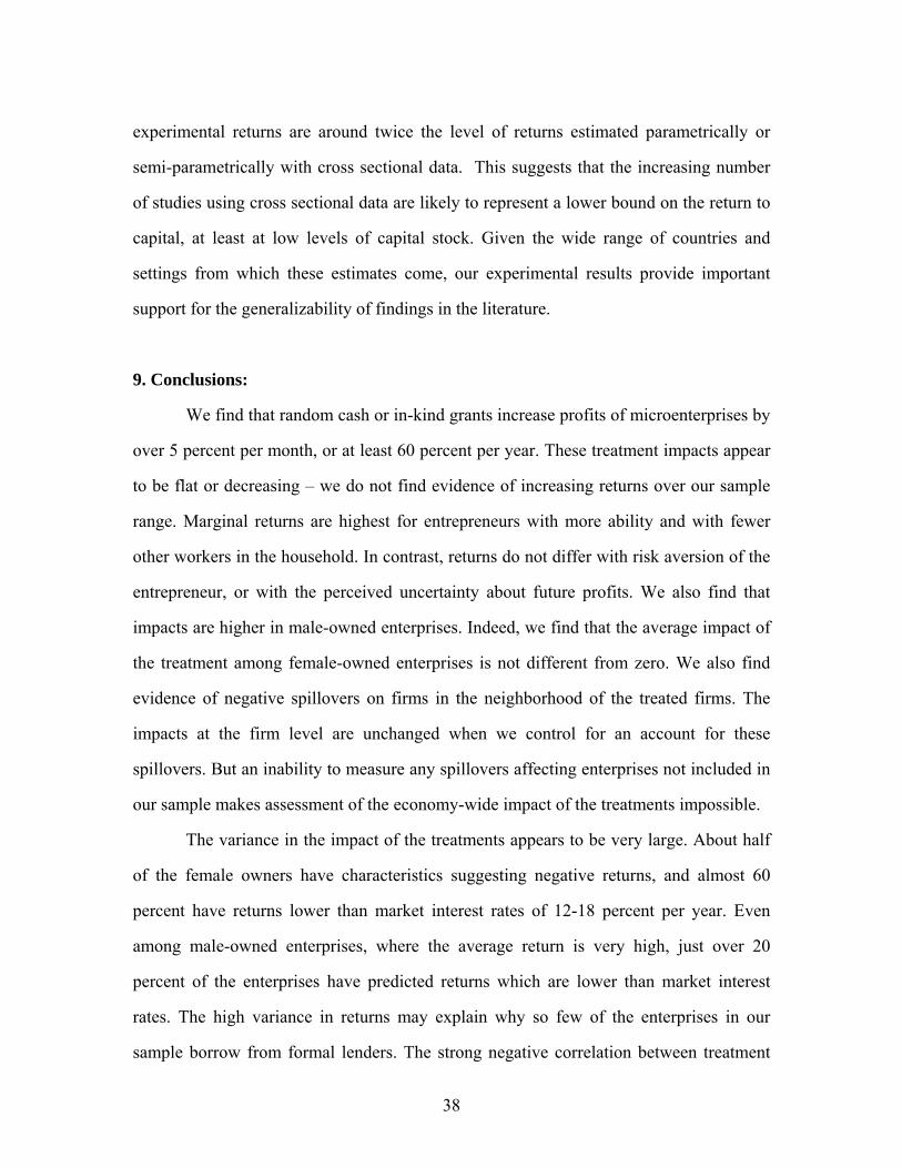
38

experimental returns are around twice the level of returns estimated parametrically or

semi-parametrically with cross sectional data. This suggests that the increasing number

of studies using cross sectional data are likely to represent a lower bound on the return to

capital, at least at low levels of capital stock. Given the wide range of countries and

settings from which these estimates come, our experimental results provide important

support for the generalizability of findings in the literature.

9. Conclusions:

We find that random cash or in-kind grants increase profits of microenterprises by

over 5 percent per month, or at least 60 percent per year. These treatment impacts appear

to be flat or decreasing – we do not find evidence of increasing returns over our sample

range. Marginal returns are highest for entrepreneurs with more ability and with fewer

other workers in the household. In contrast, returns do not differ with risk aversion of the

entrepreneur, or with the perceived uncertainty about future profits. We also find that

impacts are higher in male-owned enterprises. Indeed, we find that the average impact of

the treatment among female-owned enterprises is not different from zero. We also find

evidence of negative spillovers on firms in the neighborhood of the treated firms. The

impacts at the firm level are unchanged when we control for an account for these

spillovers. But an inability to measure any spillovers affecting enterprises not included in

our sample makes assessment of the economy-wide impact of the treatments impossible.

The variance in the impact of the treatments appears to be very large. About half

of the female owners have characteristics suggesting negative returns, and almost 60

percent have returns lower than market interest rates of 12-18 percent per year. Even

among male-owned enterprises, where the average return is very high, just over 20

percent of the enterprises have predicted returns which are lower than market interest

rates. The high variance in returns may explain why so few of the enterprises in our

sample borrow from formal lenders. The strong negative correlation between treatment

39

impact and measures of household liquidity, and the strong positive correlation between

treatment impact and ability suggest that these measures may be useful screening devices

to identify microenterprises where investments are likely to be most profitable.

The grants are associated with both an increase in capital stock and an increase in

the hours the owner works in the enterprise. Arguably, this total treatment impact, is of

most interest to lenders, who are concerned that the additional resources generate enough

profit to repay loans. But the returns to the additional capital, isolated from other impact

channels, is also of interest to discussions in the economics literature. With some

additional assumptions, we are able to use the random treatments to estimate marginal

returns to capital in the enterprises. Using different estimates of the marginal productivity

of the owner’s additional work effort, we find returns of 4.6 to 5.3 percent per month, 55-

63 percent per year. These high returns at very low levels of capital stock imply that non-

convex production sets are unlikely to lead to permanent poverty traps. One caveat to this

optimistic conclusion is that our sample includes only individuals who ran an enterprise

at the time of the baseline sample. Entry may be prevented not by a requirement to invest

a large amount of capital, but by the possibility of an initial period of very low

profitability. Our data do not allow us to examine this possibility.

Although the variance in returns may limit the willingness of banks to lend to

these firms, we still view the high level of returns as something of a puzzle. The majority

of the treatments were invested in working capital. If returns to these investments are so

high, what prevents firms from growing incrementally by reinvesting profits? Is it a lack

of savings institutions—or a lack of knowledge about how the savings institutions

operate—recurrent shocks to households, or time inconsistent preferences? Because

working capital investments are unlikely to involve indivisibilities, a lack of savings

institutions by itself is unlikely to provide a full answer to this puzzle. What the results

point to is the need for a better understanding of how these microentrepreneurs make

investment decisions. We see this as a fertile area for future research.

40

Suresh de Mel, University of Peradeniya

David McKenzie, World Bank

Christopher Woodruff, University of California, San Diego

References Abadie, Alberto, Joshua Angrist and Guido Imbens (2002) "Instrumental

Variables Estimates of the Effect of Subsidized Training on the Quantiles of Trainee Earnings", Econometrica 70(1): 91-117

Armendáriz de Aghion, Beatriz and Jonathan Morduch (2005), The Economics of Microfinance, Cambridge: MIT Press.

Angrist, Joshua, Guido Imbens and Donald Rubin (1996) “Identification of Causal Effects Using Instrumental Variables”, Journal of the American Statistical Association 91: 444-55.

Aghion, Philippe and Patrick Bolton (1997) "A Theory of Trickle-Down Growth and Development", The Review of Economic Studies, 64(2): 151-172.

Banerjee, Abhijit and Esther Duflo 2004, “Do Firms want to Borrow More? Testing Credit Constraints Using a Directed Lending Program,” working paper MIT.

Banerjee, Abhijit and Esther Duflo, 2005, “Growth Theory through the Lens of Development Economics,” in Aghion and Durlauf, eds., Handbook of Economic Growth. Elsevier Press.

Banerjee, Abhijit V. and Andrew F. Newman (1993) "Occupational Choice and the Process of Development", The Journal of Political Economy 101(2): 274-298.

Bardhan, Pranab and Christopher Udry, 1999, Development Microeconomics. Oxford: Oxford University Press

Burjorjee, Deena M., Deshpande, Rani, and Weidemann, C. Jean (2002), "Supporting Women's Livelihoods Microfinance that Works for the Majority. A Guide to Best Practices", United Nations Capital Development Fund, Special Unit for Microfinance. http://www.uncdf.org/english/microfinance/pubs/thematic_papers/gender/supporting/part_1.php

Card, David (2001) “Estimating the Return to Schooling: Progress on some persistent econometric problems”, Econometrica 69(5): 1127-60.

De Mel, Suresh, David McKenzie and Christopher Woodruff, 2007. “Who does Microfinance Fail to Reach? Experimental Evidence on Gender and Microenterprise Returns”, BREAD Working Paper No.157.

______________, 2008a, “Measuring Microenterprise Profits: Must we ask how the sausage is made?,” Journal of Development Economics, forthcoming.

______________, 2008b, “Enterprise Recovery following Natural Disasters,” working paper, UCSD

Duflo, Esther, Rachel Glennerster and Michael Kremer (2006) “Using Randomization in Development Economics: A Toolkit”, BREAD Working Paper No. 136.

41

FINCA (2007), "Frequently Asked Questions", http://www.villagebanking.org/site/c.erKPI2PCIoE/b.2394157/k.8161/Frequently_Asked_Questions.htm [accessed August 15, 2007].

Gibson, John and David McKenzie (2007) “Using the Global Positioning System (GPS) in Household Surveys for Better Economics and Better Policy”, World Bank Research Observer 22(2): 217-241.

Gine, Xavier and Dean Karlan, 2007, “Group vs. Individual Liability: A Field Experiment in the Philippines,” working paper, Yale University

Khandker, Shahidur R. (1998), "Using microcredit to advance women", World Bank Premnote (November) No8. http://www1.worldbank.org/prem/PREMNotes/premnote8.pdf [accessed August 15, 2007].

Karlan, Dean, 2001, “Microfinance Impact Assessments: The Perils of Using New Members as a Control Group,” Journal of Microfinance, December 2001

Kling, Jeffrey R., Jeffrey B. Liebman and Lawrence F. Katz (2007) “Experimental Analysis of Neighborhood Effects”, Econometrica 75(1): 83-119.

Koenker, Roger (2004) "Quantile regression for longitudinal data", Journal of Multivariate Analysis 91(1): 74-89

Lee, David (2005) “Training, Wages, and Sample Selection: Estimating Sharp Bounds on Treatment Effects”, NBER Working Paper No. 11721.

Lloyd-Ellis, Huw and Dan Bernhardt (2000) "Enterprise, Inequality and Economic Development", The Review of Economic Studies 67: 147-168.

McKenzie, David and Christopher Woodruff, 2006, “Do Entry Costs Provide an Empirical Basis for Poverty Traps? Evidence from Mexican Microenterprises”, Economic Development and Cultural Change 55(1): 3-42.

McKenzie, David and Christopher Woodruff (2008) “Experimental Evidence on Returns to Capital and Access to Finance in Mexico”, Mimeo. World Bank.

Miguel, Edward and Michael Kremer (2004) “Worms: Identifying Impacts on Education and Health in the Presence of Treatment Externalities”, Econometrica 72(1): 159-217.

Morduch, Jonathan, “The Microfinance Promise,” Journal of Economic Literature, Vol. 37(4), December 1999, pp. 1569-1614.

SEAGA, Socio-economic and Gender Analysis Programme (2002), "A guide to Gender sensitive microfinance", FAO. http://www.fao.org/sd/seaga/downloads/En/Microfinanceen.pdf [accessed August 15, 2007].

Schündeln, Matthias, 2007, “Appreciating Depreciation: A Note on Physical Capital Depreciation in a Developing Country,” working paper, Harvard University.

Udry, Christopher and Santosh Anagol, 2006, “The Return to Capital in Ghana,” American Economic Review 96(2): 388-93.

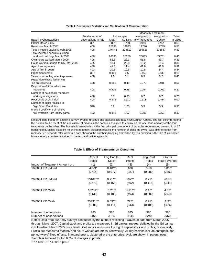
42

Total number of Assigned to Assigned to T-testBaseline Characteristic observations in R1. Mean St. Dev. any Treatment Control p-valueProfits March 2005 391 3851 3289 3919 3757 0.63Revenues March 2005 408 12193 14933 11796 12739 0.53Total invested capital March 2005 408 146441 224512 155626 133837 0.33Total invested capital excluding land and buildings March 2005 408 26530 25259 25633 27761 0.40Own hours worked March 2005 408 52.6 22.3 51.8 53.7 0.39Hours worked, unpaid family, Mar 2005 405 18.1 28.8 18.2 15.4 0.31Age of entrepreneur 408 41.8 11.4 41.8 41.9 0.92Age of firm in years 403 10.3 10.5 10.8 9.7 0.34Proportion female 387 0.491 0.5 0.459 0.533 0.15Years of schooling of entrepreneur 408 9.0 3.1 8.9 9.2 0.40Proportion whose father was an entrepreneur 408 0.385 0.49 0.373 0.401 0.56Proportion of firms which are registered 408 0.235 0.45 0.254 0.209 0.32Number of household members working in wage jobs 408 0.7 0.83 0.7 0.7 0.73Household asset index 408 0.276 1.610 0.118 0.494 0.02Number of digits recalled in Digit Span Recall test 370 5.9 1.23 5.9 5.9 0.96Implied coefficient of relative risk aversion from lottery game 403 0.143 1.57 0.206 0.053 0.33

Means by TreatmentFull sample

Note: All data based on baseline survey. Profits, revenue and capital stock data in Sri Lankan rupees. The last column reports the p-value fot he t-test of the equivalnce of means in the samples assigned to control on the one hand and any of the four treatments on the other. The household asset index is the first principal component of variables representing ownership of 17 household durables, listed int he online appendix; digitspan recall is the number of digits the owner was able to repeat from memory, ten seconds after viewing a card showing the numbers (ranging from 3 to 11); risk aversion is the CRRA calculated from a lottery exercise described in the text and online appendix.

Table I: Descriptive Statistics and Verification of Randomization

Capital Log Capital Real Log Real OwnerStock Stock Profits Profits Hours Worked

Impact of Treatment Amount on: (1) (2) (3) (4) (5)10,000 LKR In-kind 4793* 0.40*** 186 0.10 6.06**

(2714) (0.077) (387) (0.089) (2.86)

20,000 LKR In-kind 13167*** 0.71*** 1022* 0.21* -0.57(3773) (0.169) (592) (0.115) (3.41)

10,000 LKR Cash 10781** 0.23** 1421*** 0.15* 4.52*(5139) (0.103) (493) (0.080) (2.54)

20,000 LKR Cash 23431*** 0.53*** 775* 0.21* 2.37(6686) (0.111) (643) (0.109) (3.26)

Number of enterprises 385 385 385 385 385Number of observations 3155 3155 3248 3248 3378

*** p<0.01, ** p<0.05, * p<0.1

Notes: Data from quarterly surveys conducted by the authors reflecting 9 waves of data from March 2005 through March 2007. Capital stock and profits are measured in Sri Lankan rupees, deflated by the Sri Lankan CPI to reflect March 2005 price levels. Columns 2 and 4 use the log of capital stock and profits, respectively. Profits are measured monthly and hours worked are measured weekly. All regressions include enterprise and period (wave) fixed effects. Standard errors, clustered at the enterprise level, are shown in parentheses. Sample is trimmed for top 0.5% of changes in profits.

Table II: Effect of Treatments on Outcomes

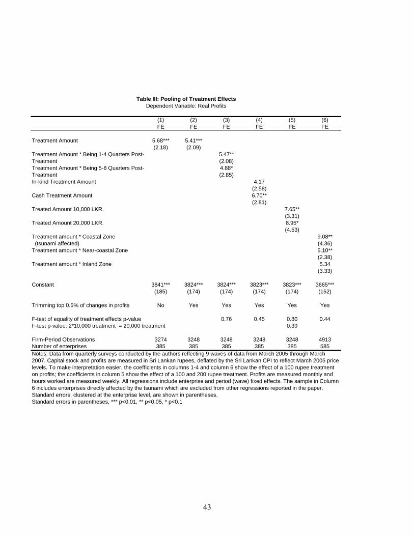
43

(1) (2) (3) (4) (5) (6)FE FE FE FE FE FE

Treatment Amount 5.68*** 5.41***(2.18) (2.09)

5.47**(2.08)4.88*(2.85)

In-kind Treatment Amount 4.17(2.58)

Cash Treatment Amount 6.70**(2.81)

Treated Amount 10,000 LKR. 7.65**(3.31)

Treated Amount 20,000 LKR. 8.95*(4.53)

Treatment amount * Coastal Zone 9.08** (tsunami affected) (4.36)Treatment amount * Near-coastal Zone 5.10**

(2.38)Treatment amount * Inland Zone 5.34

(3.33)

Constant 3841*** 3824*** 3824*** 3823*** 3823*** 3665***(185) (174) (174) (174) (174) (152)

Trimming top 0.5% of changes in profits No Yes Yes Yes Yes Yes

F-test of equality of treatment effects p-value 0.76 0.45 0.80 0.44F-test p-value: 2*10,000 treatment = 20,000 treatment 0.39

Firm-Period Observations 3274 3248 3248 3248 3248 4913Number of enterprises 385 385 385 385 385 585

Standard errors in parentheses, *** p<0.01, ** p<0.05, * p<0.1

Notes: Data from quarterly surveys conducted by the authors reflecting 9 waves of data from March 2005 through March 2007. Capital stock and profits are measured in Sri Lankan rupees, deflated by the Sri Lankan CPI to reflect March 2005 price levels. To make interpretation easier, the coefficients in columns 1-4 and column 6 show the effect of a 100 rupee treatment on profits; the coefficients in column 5 show the effect of a 100 and 200 rupee treatment. Profits are measured monthly and hours worked are measured weekly. All regressions include enterprise and period (wave) fixed effects. The sample in Column 6 includes enterprises directly affected by the tsunami which are excluded from other regressions reported in the paper. Standard errors, clustered at the enterprise level, are shown in parentheses.

Treatment Amount * Being 1-4 Quarters Post-TreatmentTreatment Amount * Being 5-8 Quarters Post-Treatment

Table III: Pooling of Treatment EffectsDependent Variable: Real Profits

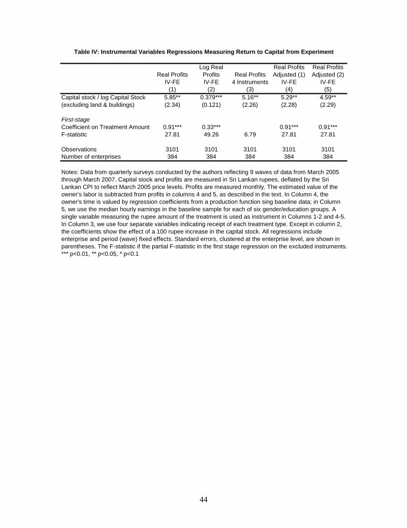
44

IV-FE IV-FE 4 Instruments IV-FE IV-FE(1) (2) (3) (4) (5)

Capital stock / log Capital Stock 5.85** 0.379*** 5.16** 5.29** 4.59**(excluding land & buildings) (2.34) (0.121) (2.26) (2.28) (2.29)

First-stageCoefficient on Treatment Amount 0.91*** 0.33*** 0.91*** 0.91***F-statistic 27.81 49.26 6.79 27.81 27.81

Observations 3101 3101 3101 3101 3101Number of enterprises 384 384 384 384 384

*** p<0.01, ** p<0.05, * p<0.1

Table IV: Instrumental Variables Regressions Measuring Return to Capital from Experiment

Real Profits Adjusted (2)Real ProfitsReal Profits

Log Real Profits

Real Profits Adjusted (1)

Notes: Data from quarterly surveys conducted by the authors reflecting 9 waves of data from March 2005 through March 2007. Capital stock and profits are measured in Sri Lankan rupees, deflated by the Sri Lankan CPI to reflect March 2005 price levels. Profits are measured monthly. The estimated value of the owner's labor is subtracted from profits in columns 4 and 5, as described in the text. In Column 4, the owner's time is valued by regression coefficients from a production function sing baseline data; in Column 5, we use the median hourly earnings in the baseline sample for each of six gender/education groups. A single variable measuring the rupee amount of the treatment is used as instrument in Columns 1-2 and 4-5. In Column 3, we use four separate variables indicating receipt of each treatment type. Except in column 2, the coefficients show the effect of a 100 rupee increase in the capital stock. All regressions include enterprise and period (wave) fixed effects. Standard errors, clustered at the enterprise level, are shown in parentheses. The F-statistic if the partial F-statistic in the first stage regression on the excluded instruments.

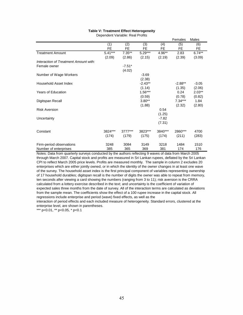
45

Females Males(1) (2) (3) (4) (5) (6)FE FE FE FE FE FE

Treatment Amount 5.41*** 7.35** 5.29*** 4.96** 2.83 6.74**(2.09) (2.86) (2.15) (2.19) (2.39) (3.09)

Interaction of Treatment Amount with:Female owner -7.51*

(4.02)Number of Wage Workers -3.69

(2.38)Household Asset Index -2.43** -2.88** -3.05

(1.14) (1.35) (2.06)Years of Education 1.56*** 0.24 2.03**

(0.59) (0.78) (0.82)Digitspan Recall 3.80** 7.34*** 1.84

(1.88) (2.32) (2.80)Risk Aversion 0.54

(1.25)Uncertainty -7.82

(7.31)

Constant 3824*** 3777*** 3823*** 3840*** 2860*** 4700(174) (179) (175) (174) (211) (283)

Firm-period observations 3248 3084 3149 3218 1484 1510Number of enterprises 385 365 369 381 174 176

*** p<0.01, ** p<0.05, * p<0.1

Notes: Data from quarterly surveys conducted by the authors reflecting 9 waves of data from March 2005 through March 2007. Capital stock and profits are measured in Sri Lankan rupees, deflated by the Sri Lankan CPI to reflect March 2005 price levels. Profits are measured monthly. The sample in column 2 excludes 20 enterprises which are either jointly owned, or in which the identity of the owner changes in at least one wave of the survey. The household asset index is the first principal component of variables representing ownership of 17 household durables; digitspan recall is the number of digits the owner was able to repeat from memory, ten seconds after viewing a card showing the numbers (ranging from 3 to 11); risk aversion is the CRRA calculated from a lottery exercise described in the text; and uncertainty is the coefficient of variation of expected sales three months from the date of survey. All of the interaction terms are calculated as deviations from the sample mean. The coefficients show the effect of a 100 rupee increase in the capital stock. All regressions include enterprise and period (wave) fixed effects, as well as the interaction of period effects and each included measure of heterogeneity. Standard errors, clustered at the enterprise level, are shown in parentheses.

Table V: Treatment Effect HeterogeneityDependent Variable: Real Profits

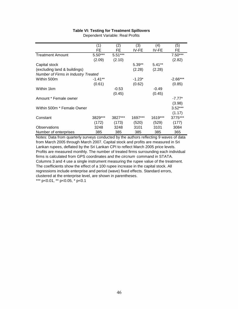
46

(1) (2) (3) (4) (5)FE FE IV-FE IV-FE FE

Treatment Amount 5.50*** 5.51*** 7.50***(2.09) (2.10) (2.82)

Capital stock 5.39** 5.41**(excluding land & buildings) (2.28) (2.28)Number of Firms in Industry TreatedWithin 500m -1.41** -1.23* -2.66***

(0.61) (0.62) (0.85)Within 1km -0.53 -0.49

(0.45) (0.45)Amount * Female owner -7.77*

(3.98)Within 500m * Female Owner 3.52***

(1.17)Constant 3829*** 3827*** 1697*** 1619*** 3775***

(172) (173) (520) (529) (177)Observations 3248 3248 3101 3101 3084Number of enterprises 385 385 385 385 365

*** p<0.01, ** p<0.05, * p<0.1

Notes: Data from quarterly surveys conducted by the authors reflecting 9 waves of data from March 2005 through March 2007. Capital stock and profits are measured in Sri Lankan rupees, deflated by the Sri Lankan CPI to reflect March 2005 price levels. Profits are measured monthly. The number of treated firms surrounding each individual firms is calculated from GPS coordinates and the circnum command in STATA. Columns 3 and 4 use a single instrument measuring the rupee value of the treatment. The coefficients show the effect of a 100 rupee increase in the capital stock. All regressions include enterprise and period (wave) fixed effects. Standard errors, clustered at the enterprise level, are shown in parentheses.

Table VI: Testing for Treatment SpilloversDependent Variable: Real Profits

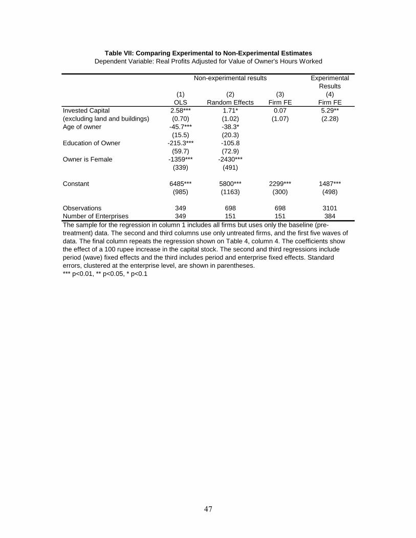
47

(1) (2) (3) (4)OLS Random Effects Firm FE Firm FE

Invested Capital 2.58*** 1.71* 0.07 5.29**(excluding land and buildings) (0.70) (1.02) (1.07) (2.28)Age of owner -45.7*** -38.3*

(15.5) (20.3)Education of Owner -215.3*** -105.8

(59.7) (72.9)Owner is Female -1359*** -2430***

(339) (491)

Constant 6485*** 5800*** 2299*** 1487***(985) (1163) (300) (498)

Observations 349 698 698 3101Number of Enterprises 349 151 151 384

*** p<0.01, ** p<0.05, * p<0.1

Non-experimental results Experimental Results

The sample for the regression in column 1 includes all firms but uses only the baseline (pre-treatment) data. The second and third columns use only untreated firms, and the first five waves of data. The final column repeats the regression shown on Table 4, column 4. The coefficients show the effect of a 100 rupee increase in the capital stock. The second and third regressions include period (wave) fixed effects and the third includes period and enterprise fixed effects. Standard errors, clustered at the enterprise level, are shown in parentheses.

Table VII: Comparing Experimental to Non-Experimental EstimatesDependent Variable: Real Profits Adjusted for Value of Owner's Hours Worked

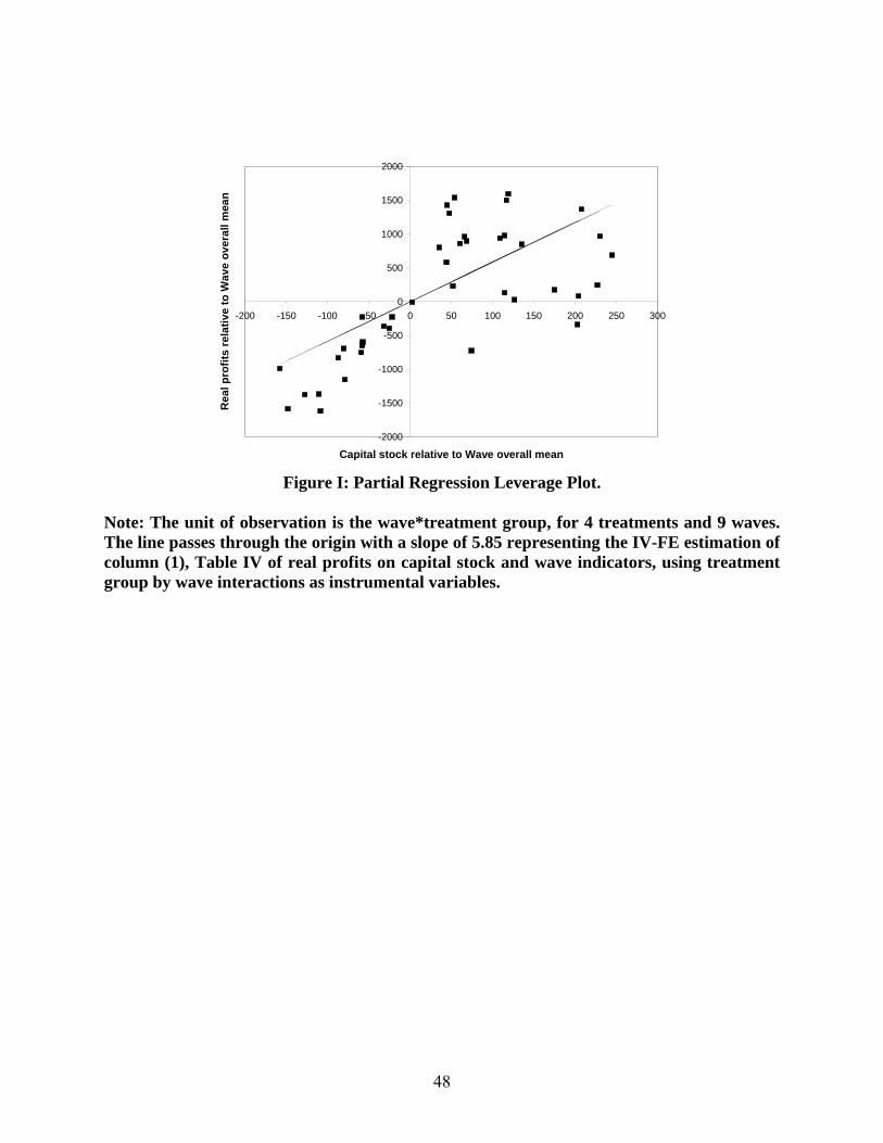
48

-2000

-1500

-1000

-500

0

500

1000

1500

2000

-200 -150 -100 -50 0 50 100 150 200 250 300

Capital stock relative to Wave overall mean

Rea

l pro

fits

rela

tive

to W

ave

over

all m

ean

Figure I: Partial Regression Leverage Plot.

Note: The unit of observation is the wave*treatment group, for 4 treatments and 9 waves. The line passes through the origin with a slope of 5.85 representing the IV-FE estimation of column (1), Table IV of real profits on capital stock and wave indicators, using treatment group by wave interactions as instrumental variables.