Embed Size (px)
Citation preview
REVERSE CENTRALITY QUERIES IN COMPLEX
NETWORKS
by
Brittany Nielsen
B.Sc. (Hons.), Simon Fraser University, 2007
a Thesis submitted in partial fulfillment
of the requirements for the degree of
Master of Science
in the School
of
Computing Science
c⃝ Brittany Nielsen 2009
SIMON FRASER UNIVERSITY
Fall 2009
All rights reserved. This work may not be
reproduced in whole or in part, by photocopy
or other means, without the permission of the author.

Last revision: Spring 09
Declaration of Partial Copyright Licence The author, whose copyright is declared on the title page of this work, has granted to Simon Fraser University the right to lend this thesis, project or extended essay to users of the Simon Fraser University Library, and to make partial or single copies only for such users or in response to a request from the library of any other university, or other educational institution, on its own behalf or for one of its users.
The author has further granted permission to Simon Fraser University to keep or make a digital copy for use in its circulating collection (currently available to the public at the “Institutional Repository” link of the SFU Library website <www.lib.sfu.ca> at: <http://ir.lib.sfu.ca/handle/1892/112>) and, without changing the content, to translate the thesis/project or extended essays, if technically possible, to any medium or format for the purpose of preservation of the digital work.
The author has further agreed that permission for multiple copying of this work for scholarly purposes may be granted by either the author or the Dean of Graduate Studies.
It is understood that copying or publication of this work for financial gain shall not be allowed without the author’s written permission.
Permission for public performance, or limited permission for private scholarly use, of any multimedia materials forming part of this work, may have been granted by the author. This information may be found on the separately catalogued multimedia material and in the signed Partial Copyright Licence.
While licensing SFU to permit the above uses, the author retains copyright in the thesis, project or extended essays, including the right to change the work for subsequent purposes, including editing and publishing the work in whole or in part, and licensing other parties, as the author may desire.
The original Partial Copyright Licence attesting to these terms, and signed by this author, may be found in the original bound copy of this work, retained in the Simon Fraser University Archive.
Simon Fraser University Library Burnaby, BC, Canada
Abstract
The increasing availability of complex network data from social networks and other sources
provides new opportunities for exploration and analysis. In this thesis, we introduce the
reverse centrality query, a novel query for complex networks. For a query node q, the reverse
centrality query returns a locally maximal induced subgraph R, where q ∈ R, such that q
dominates R according to a centrality index C. Many centrality indices have been introduced
to describe the relationships between nodes in complex networks. We focus on degree,
graph, and closeness centrality indices and their respective reverse graph centrality queries.
The theoretical properties of these queries, together with heuristic variants, are explored.
Algorithms for solving these queries are given and experimental results are provided on
three real world datasets. The experiments demonstrate reverse centrality queries to be a
useful tool for social network analysis.
iii

To Geoff
iv

“Ohne Fleiß, kein Preis.”
— German proverb
v

Acknowledgments
I would particularly like to thank my senior supervisor Dr. Jian Pei for his dedication
and creativeness in helping me pursue this thesis through from initial idea, through many
iterations, to its final completion.
I would like to express my gratitude to Dr. Ke Wang for serving as my supervisor and
taking great care in reading and critiquing my thesis.
Many thanks to Dr. Oliver Schulte for serving as examiner on my committee.
Thanks to Kate Tsoukalas, Ming Hua, and Crystal Xing and the other members of the
lab for generous feedback, help and suggestions throughout my masters program.
I would like to give special acknowledgement to NSERC for providing funding which
directly supported my graduate studies.
Thank you to my family and friends who accepted my occasional absence due to com-
mitments to my graduate studies.
Finally, a special thank you to Geoff for offering suggestions, encouragement, and support
throughout the writing process.
vi

Contents
Approval ii
Abstract iii
Dedication iv
Quotation v
Acknowledgments vi
Contents vii
List of Figures x
List of Algorithms xii
1 Introduction 1
1.1 Contributions . . . . . . . . . . . . . . . . . . . . . . . . . . . . . . . . . . . . 4
1.2 Outline . . . . . . . . . . . . . . . . . . . . . . . . . . . . . . . . . . . . . . . 4
2 Problem Definitions and Related Work 6
2.1 Preliminaries . . . . . . . . . . . . . . . . . . . . . . . . . . . . . . . . . . . . 6
2.2 Complex networks . . . . . . . . . . . . . . . . . . . . . . . . . . . . . . . . . 8
2.2.1 Definition of a complex network . . . . . . . . . . . . . . . . . . . . . 8
2.2.2 Examples of complex networks in real life . . . . . . . . . . . . . . . . 8
2.2.3 Structural properties of complex networks . . . . . . . . . . . . . . . . 10
2.3 Queries in networks . . . . . . . . . . . . . . . . . . . . . . . . . . . . . . . . 11
vii
2.4 Clustering and community finding . . . . . . . . . . . . . . . . . . . . . . . . 11
2.4.1 Related work on node queries . . . . . . . . . . . . . . . . . . . . . . . 13
2.5 Centrality indices . . . . . . . . . . . . . . . . . . . . . . . . . . . . . . . . . . 14
2.5.1 Degree-based centrality indices . . . . . . . . . . . . . . . . . . . . . . 14
2.5.2 Distance-based centrality indices . . . . . . . . . . . . . . . . . . . . . 15
2.5.3 Path-based centrality indices . . . . . . . . . . . . . . . . . . . . . . . 16
2.6 Problem definitions . . . . . . . . . . . . . . . . . . . . . . . . . . . . . . . . . 18
2.6.1 Reverse centrality queries . . . . . . . . . . . . . . . . . . . . . . . . . 18
2.6.2 Local centrality dominance . . . . . . . . . . . . . . . . . . . . . . . . 18
2.6.3 Reverse degree centrality query . . . . . . . . . . . . . . . . . . . . . . 19
2.6.4 Reverse closeness centrality query . . . . . . . . . . . . . . . . . . . . 21
2.6.5 Reverse graph centrality query . . . . . . . . . . . . . . . . . . . . . . 22
2.6.6 Constrained queries . . . . . . . . . . . . . . . . . . . . . . . . . . . . 23
3 Reverse Centrality Queries: Algorithms 25
3.1 Reverse degree centrality query . . . . . . . . . . . . . . . . . . . . . . . . . . 27
3.1.1 One-phase incremental algorithm . . . . . . . . . . . . . . . . . . . . . 28
3.1.2 Two-phase incremental algorithm . . . . . . . . . . . . . . . . . . . . . 29
3.1.3 Degree centrality neighbourhood dominance query . . . . . . . . . . . 30
3.2 Reverse closeness centrality query . . . . . . . . . . . . . . . . . . . . . . . . . 31
3.2.1 Incremental algorithm . . . . . . . . . . . . . . . . . . . . . . . . . . . 33
3.2.2 Heuristics . . . . . . . . . . . . . . . . . . . . . . . . . . . . . . . . . . 37
3.3 Reverse graph centrality query . . . . . . . . . . . . . . . . . . . . . . . . . . 38
3.3.1 Incremental algorithm . . . . . . . . . . . . . . . . . . . . . . . . . . . 40
3.3.2 Heuristics . . . . . . . . . . . . . . . . . . . . . . . . . . . . . . . . . . 42
4 Experimental Results and Discussion 43
4.1 Datasets . . . . . . . . . . . . . . . . . . . . . . . . . . . . . . . . . . . . . . . 43
4.2 Implementation . . . . . . . . . . . . . . . . . . . . . . . . . . . . . . . . . . . 44
4.3 Experimental results . . . . . . . . . . . . . . . . . . . . . . . . . . . . . . . . 45
4.3.1 Reverse degree centrality query results . . . . . . . . . . . . . . . . . . 45
4.3.2 Reverse closeness centrality query results . . . . . . . . . . . . . . . . 47
4.3.3 Reverse graph centrality results . . . . . . . . . . . . . . . . . . . . . . 54
4.3.4 Reverse centrality queries versus global centrality . . . . . . . . . . . . 61
viii
4.4 Summary . . . . . . . . . . . . . . . . . . . . . . . . . . . . . . . . . . . . . . 61
5 Conclusion and Future Work 63
5.1 Summary . . . . . . . . . . . . . . . . . . . . . . . . . . . . . . . . . . . . . . 63
5.2 Future work . . . . . . . . . . . . . . . . . . . . . . . . . . . . . . . . . . . . . 64
5.2.1 Heuristic improvements . . . . . . . . . . . . . . . . . . . . . . . . . . 64
5.2.2 Feature vector networks . . . . . . . . . . . . . . . . . . . . . . . . . . 65
5.2.3 Advanced search methods . . . . . . . . . . . . . . . . . . . . . . . . . 65
5.2.4 Variants on reverse centrality query answering . . . . . . . . . . . . . 65
5.2.5 Local Centrality Measures . . . . . . . . . . . . . . . . . . . . . . . . . 66
A Appendix 1 67
A.1 The All-Pairs Shortest Path (APSP) Problem . . . . . . . . . . . . . . . . . . 67
A.1.1 Changing Distances: Dynamic All-pairs Shortest Path . . . . . . . . . 68
Bibliography 70
ix
List of Figures
1.1 Visualization of the Les Miserables complex network . . . . . . . . . . . . . . 2
1.2 Example of a reverse centrality query result . . . . . . . . . . . . . . . . . . . 3
2.1 Visualization of the Zachary karate club network . . . . . . . . . . . . . . . . 9
3.1 Visualization of a star graph with 20 nodes . . . . . . . . . . . . . . . . . . . 26
3.2 Reverse degree centrality query result for Cosette . . . . . . . . . . . . . . . . 30
3.3 Toy example proving non-dominance . . . . . . . . . . . . . . . . . . . . . . . 32
3.4 Reverse closeness centrality query result for Cosette . . . . . . . . . . . . . . 37
3.5 Reverse graph centrality query result for Cosette . . . . . . . . . . . . . . . . 42
4.1 Degree Distribution of Sample Datasets . . . . . . . . . . . . . . . . . . . . . 44
4.2 Result Size v. Time (Degree Centrality) . . . . . . . . . . . . . . . . . . . . . 46
4.3 Degree of q v. Result Size (Degree Centrality) . . . . . . . . . . . . . . . . . . 46
4.4 Result Size v. Time (Closeness Centrality) . . . . . . . . . . . . . . . . . . . . 47
4.5 Global Centrality v. Result Size (Closeness Centrality) . . . . . . . . . . . . . 48
4.6 Candidates Tested v. Time (Closeness Centrality) . . . . . . . . . . . . . . . 48
4.7 Candidates Tested v. Successful Candidates (Closeness Centrality) . . . . . . 49
4.8 Modularity v. Result Size (Closeness Centrality) . . . . . . . . . . . . . . . . 50
4.9 Transitivity v. Result Size (Closeness Centrality) . . . . . . . . . . . . . . . . 50
4.10 Result Size v. Time (Closeness Centrality): 1 Chance . . . . . . . . . . . . . 51
4.11 Result Size v. Time (Closeness Centrality): Sorting . . . . . . . . . . . . . . . 52
4.12 Comparison of result sizes for variants (Closeness Centrality) . . . . . . . . . 53
4.13 Global Centrality v. Result Size (Graph Centrality) . . . . . . . . . . . . . . 54
4.14 Modularity v. Result Size (Graph Centrality) . . . . . . . . . . . . . . . . . . 55
4.15 Result Size v. Time (Graph Centrality) . . . . . . . . . . . . . . . . . . . . . 55
x
4.16 Transitivity v. Result Size (Graph Centrality) . . . . . . . . . . . . . . . . . . 56
4.17 Candidates Tested v. Time (Graph Centrality) . . . . . . . . . . . . . . . . . 56
4.18 Candidates tested v. Successful candidates (Graph Centrality) . . . . . . . . 57
4.19 Result Size v. Time (Graph Centrality): 1 Chance . . . . . . . . . . . . . . . 58
4.20 Result Size v. Time (Graph Centrality): Sorting . . . . . . . . . . . . . . . . 59
4.21 Comparison of result sizes for variants (Graph Centrality) . . . . . . . . . . . 60
xi

List of Algorithms
1 One-phase incremental algorithm for reverse degree centrality . . . . . . . . . . 29
2 Incremental algorithm for reverse closeness centrality: Initialization . . . . . . 35
3 Incremental algorithm for reverse closeness centrality: Growth . . . . . . . . . 36
4 Incremental algorithm for reverse graph centrality: Initialization . . . . . . . . 40
5 Incremental algorithm for reverse graph centrality: Growth . . . . . . . . . . . 41
xii
Chapter 1
Introduction
Imagine that a detective has infiltrated a crime syndicate and collected information about
the web of connections between members of the syndicate. As an investigator, you want
to utilize this information to gain a deeper understanding of the relationships between
members. One natural question to ask is: for a targeted member, what is the relationship
between this member and those to whom he is connected? This thesis describes a novel
means for understanding the local relationships between an individual and his neighbours.
The advent of widespread data storage and information processing has led to an infor-
mation explosion. For instance, the Internet is predicted to double in size every 5.3 years
[53]. The increasing availability of information provides analysts with new opportunities
to evaluate data to generate new conclusions. One area of significant growth is in social
networks, where data is most naturally represented using a graph structure.
Graph data is a format where entities are stored as nodes and relationships between the
entities are represented by links in a graph. Many domains have natural datasets which
may be represented as graphs. Datasets as diverse as social networks, protein co-expression
data, co-authorship data from peer-reviewed journals, and bank transaction records may all
be viewed as graphs. The lack of a regular order and natural complexity of the structure of
these graphs leads to the common term complex networks.
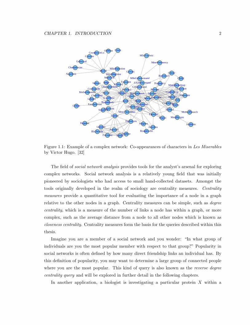
Figure 1.1 shows a small complex network, illustrating co-appearances of characters in a
Victor Hugo novel. In this small example, we can see the complex network of relationships
between individuals. Within the context of this example, our interests lay in understanding
the role of the individual character within the larger context of the network in which he
appears. The Les Miserables network will be examined in more detail in Chapter 4.
1
CHAPTER 1. INTRODUCTION 2
MyrielNapoleon
MlleBaptistine
MmeMagloire
CountessDeLo
Geborand
Champtercier
Cravatte
CountOldMan
Labarre
Valjean
Marguerite
MmeDeR
Isabeau
Gervais
Tholomyes
ListolierFameuil
Blacheville
Favourite DahliaZephine
Fantine
MmeThenardierThenardier
Cosette
JavertFauchelevent
Bamatabois
Perpetue
Simplice
Scaufflaire
Woman1
Judge
Champmathieu
BrevetChenildieu
Cochepaille
Pontmercy
Boulatruelle
Eponine
Anzelma
Woman2
MotherInnocent
Gribier
Jondrette
MmeBurgon
Gavroche
Gillenormand
Magnon
MlleGillenormand
MmePontmercy
MlleVaubois
LtGillenormand
Marius
BaronessT
Mabeuf
EnjolrasCombeferre
Prouvaire
FeuillyCourfeyrac
Bahorel
Bossuet
Joly
Grantaire
MotherPlutarch
GueulemerBabet
Claquesous
Montparnasse
ToussaintChild1
Child2
Brujon
MmeHucheloup
Figure 1.1: Example of a complex network: Co-appearances of characters in Les Miserablesby Victor Hugo. [32]
The field of social network analysis provides tools for the analyst’s arsenal for exploring
complex networks. Social network analysis is a relatively young field that was initially
pioneered by sociologists who had access to small hand-collected datasets. Amongst the
tools originally developed in the realm of sociology are centrality measures. Centrality
measures provide a quantitative tool for evaluating the importance of a node in a graph
relative to the other nodes in a graph. Centrality measures can be simple, such as degree
centrality, which is a measure of the number of links a node has within a graph, or more
complex, such as the average distance from a node to all other nodes which is known as
closeness centrality. Centrality measures form the basis for the queries described within this
thesis.
Imagine you are a member of a social network and you wonder: “In what group of
individuals are you the most popular member with respect to that group?” Popularity in
social networks is often defined by how many direct friendship links an individual has. By
this definition of popularity, you may want to determine a large group of connected people
where you are the most popular. This kind of query is also known as the reverse degree
centrality query and will be explored in further detail in the following chapters.
In another application, a biologist is investigating a particular protein X within a
CHAPTER 1. INTRODUCTION 3
protein-protein interaction network, in particular, she is interested in understanding and
exploring the relationship of that protein with others in the network. One interesting query
may be to find the group of proteins that the protein X is most central to, where it has the
shortest average distance to all other proteins within the group. This group of proteins is
centered on the query protein X, and as such provides a more meaningful description of the
vicinity of X than the set of all neighbours of X or the set of all proteins within distance 2.
This type of query is answered by the reverse closeness centrality query, which is explored
in further depth within the thesis.
In this thesis, we are interested in determining a region of dominance for a query node,
where the query node q is not outranked by any other node according to a given centrality
measure. The node q is called locally dominant in the region. By exploring this problem,
we provide a new avenue for the exploration of complex networks.
Due to the exponential number of induced subgraphs in a graph, the search space for this
problem is massive, providing an efficient solution to the reverse centrality query problem
will not be trivial.
0
1
2
3
4
5
6
78
9
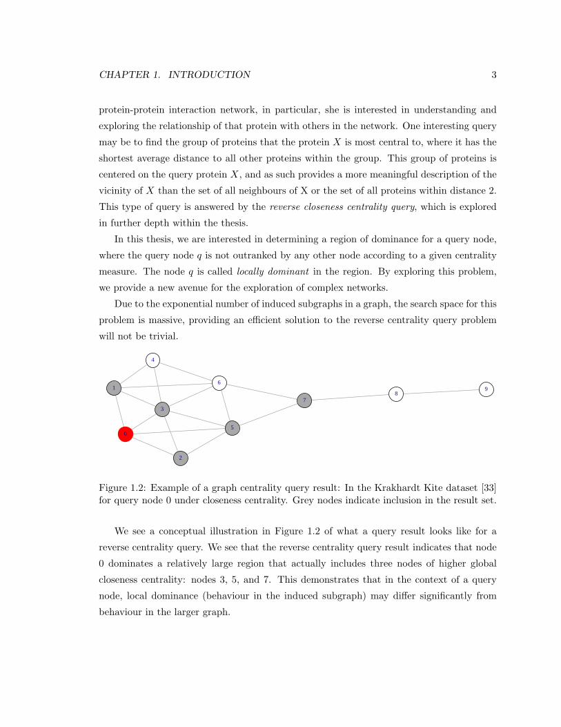
Figure 1.2: Example of a graph centrality query result: In the Krakhardt Kite dataset [33]for query node 0 under closeness centrality. Grey nodes indicate inclusion in the result set.
We see a conceptual illustration in Figure 1.2 of what a query result looks like for a
reverse centrality query. We see that the reverse centrality query result indicates that node
0 dominates a relatively large region that actually includes three nodes of higher global
closeness centrality: nodes 3, 5, and 7. This demonstrates that in the context of a query
node, local dominance (behaviour in the induced subgraph) may differ significantly from
behaviour in the larger graph.
CHAPTER 1. INTRODUCTION 4
1.1 Contributions
The main contribution of this thesis is the introduction of a new type of query for complex
networks: the reverse centrality query. In particular, three specific types of reverse centrality
queries are explored, based on degree centrality, closeness centrality, and graph centrality,
respectively. We present practical incremental algorithms for finding locally maximal regions
of dominance for these three types of the reverse centrality query. Following this, we give
experimental results on real-world datasets, showing the application and behaviour of the
implemented algorithms. Finally, we offer future directions for reverse centrality queries for
exploration and development.
Furthermore, we provide a detailed analysis of centrality measures and their relation-
ships to one another. We explore and describe the existing algorithms for global centrality
measure calculations. In addition, we provide an introduction to complex networks and
social network analysis for those unfamiliar with the field.
In more detail, the contributions of this thesis include the following aspects. We pro-
vide the general framework for reverse centrality queries: a framework that allows for the
definition of a reverse centrality query irrespective of the centrality measure used. We give
detailed formal problem definitions for reverse centrality queries based on three different
centrality measures: degree, graph and closeness centrality. We provide a detailed practical
incremental algorithm for each query type and discuss the expected characteristics of each
algorithm. For each query type, formal proofs of the behaviour of the query are given.
We describe and explore practical algorithmic solutions for these queries using real world
graphs and provide detailed analysis of the results. Applications of these novel query types
are given for several domains, including marketing, social network analysis, and computer
network analysis. In addition, we provide and analyze several heuristics to improve query
speed and result quality. Finally, we explore limitations of the methods given in this thesis
and provide suggestions for future work on reverse centrality queries.
1.2 Outline
A brief outline of the contents of the following chapters:
• Chapter 2 contains related work in social network analysis and definitions used for
the rest of the thesis. Following that, we give formal problem definitions for reverse
CHAPTER 1. INTRODUCTION 5
centrality queries.
• Chapter 3 presents algorithms for implementing three types of reverse centrality
queries. In addition, we present several variations on the basic methods to improve
query time as well as query quality.
• Chapter 4 provides experimental results for three real world datasets showing the
query behaviour and applicability of the reverse centrality queries. The behaviour of
several algorithmic variants is also explored and analyzed.
• Chapter 5 gives the limitations of the work presented in this thesis, options for future
work and a summarization of the contents of the thesis.
• Appendix 1 describes related work in the all-pairs shortest path problem from graph
theory that is related to calculating reverse centrality queries.
Chapter 2
Problem Definitions and Related
Work
In this chapter, we introduce complex networks and several areas of research in social net-
work analysis related to this study. Furthermore, community detection and cluster finding
algorithms are explored and described. We describe several families of centrality indices,
based on degree, distance and paths, and give a brief description of related work.
We also introduce reverse centrality queries and then describe several constraints that
may be placed on queries. Formal problem definitions for the reverse centrality queries
are provided for three centrality indices: degree, graph and closeness centrality. We also
describe several applications for each of the introduced reverse centrality queries.
2.1 Preliminaries
In this section, we introduce some of the preliminary definitions that are required for for-
malizing the reverse graph centrality problem.
Definition 2.1.1. A graph, G = (V,E) is a mathematical structure consisting of a set V
of vertices and a set E of edges, where an edge connects a pair of vertices. These vertices
and edges are alternatively known as nodes and links. In an undirected graph, edges have
no direction, so the edge (a, b) indicates a link between a and b and visa versa.
Definition 2.1.2. Given a graph G = (V,E) and two vertices, s, t ∈ G, a geodesic path
is the shortest path in the graph from s to t, which is measured by the number of edges
6
CHAPTER 2. PROBLEM DEFINITIONS AND RELATED WORK 7
contained in the path. The network distance is defined as the length of a geodesic path
between two vertices. The notation used for the distance between vertices s and t is d(s, t).
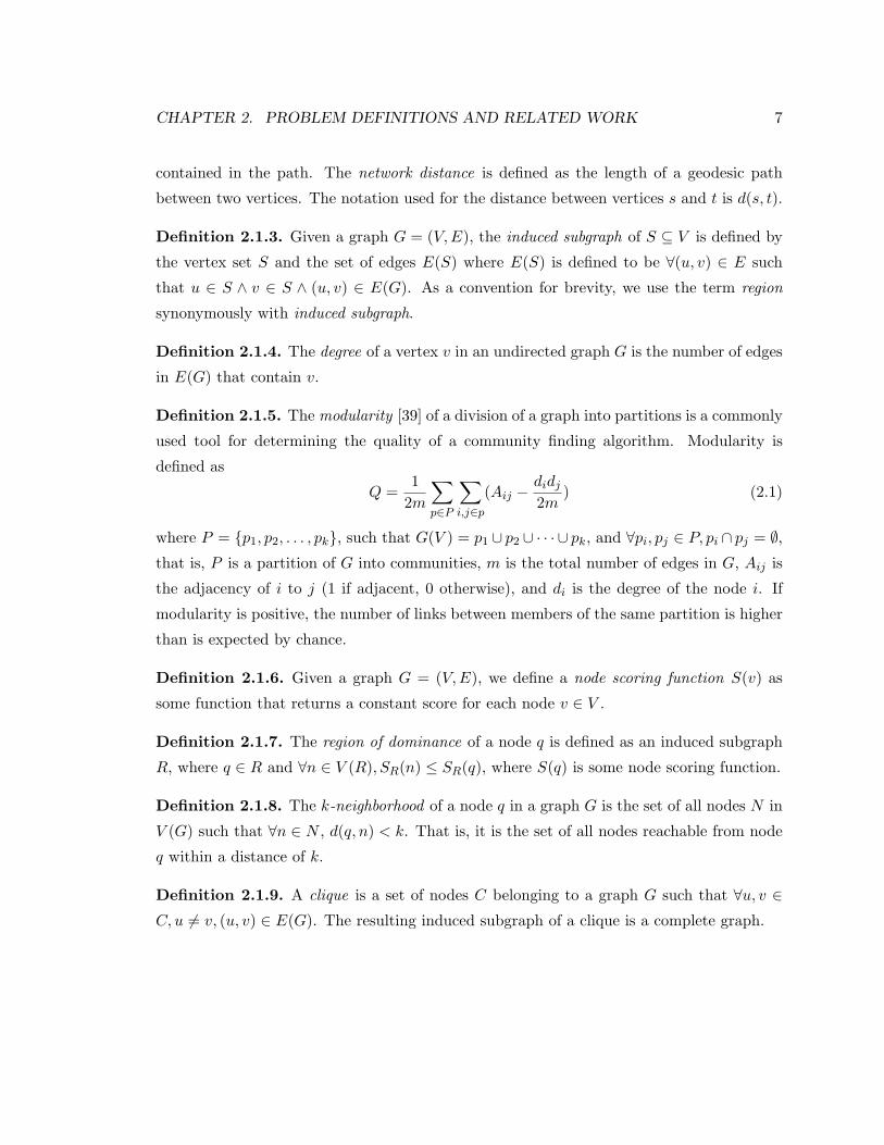
Definition 2.1.3. Given a graph G = (V,E), the induced subgraph of S ⊆ V is defined by
the vertex set S and the set of edges E(S) where E(S) is defined to be ∀(u, v) ∈ E such
that u ∈ S ∧ v ∈ S ∧ (u, v) ∈ E(G). As a convention for brevity, we use the term region
synonymously with induced subgraph.
Definition 2.1.4. The degree of a vertex v in an undirected graph G is the number of edges
in E(G) that contain v.
Definition 2.1.5. The modularity [39] of a division of a graph into partitions is a commonly
used tool for determining the quality of a community finding algorithm. Modularity is
defined as
Q =1
2m
∑p∈P
∑i,j∈p
(Aij −didj2m
) (2.1)
where P = {p1, p2, . . . , pk}, such that G(V ) = p1 ∪ p2 ∪ · · · ∪ pk, and ∀pi, pj ∈ P, pi ∩ pj = ∅,that is, P is a partition of G into communities, m is the total number of edges in G, Aij is
the adjacency of i to j (1 if adjacent, 0 otherwise), and di is the degree of the node i. If
modularity is positive, the number of links between members of the same partition is higher
than is expected by chance.
Definition 2.1.6. Given a graph G = (V,E), we define a node scoring function S(v) as
some function that returns a constant score for each node v ∈ V .
Definition 2.1.7. The region of dominance of a node q is defined as an induced subgraph
R, where q ∈ R and ∀n ∈ V (R), SR(n) ≤ SR(q), where S(q) is some node scoring function.
Definition 2.1.8. The k-neighborhood of a node q in a graph G is the set of all nodes N in
V (G) such that ∀n ∈ N , d(q, n) < k. That is, it is the set of all nodes reachable from node
q within a distance of k.
Definition 2.1.9. A clique is a set of nodes C belonging to a graph G such that ∀u, v ∈C, u = v, (u, v) ∈ E(G). The resulting induced subgraph of a clique is a complete graph.
CHAPTER 2. PROBLEM DEFINITIONS AND RELATED WORK 8
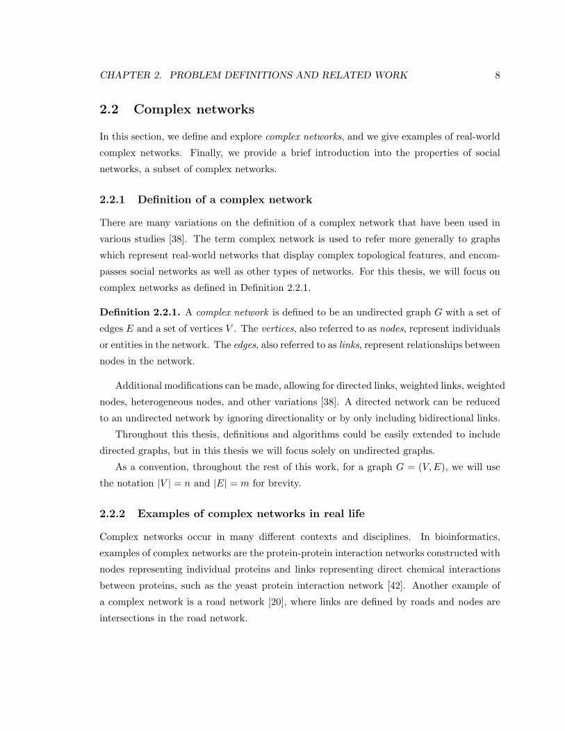
2.2 Complex networks
In this section, we define and explore complex networks, and we give examples of real-world
complex networks. Finally, we provide a brief introduction into the properties of social
networks, a subset of complex networks.
2.2.1 Definition of a complex network
There are many variations on the definition of a complex network that have been used in
various studies [38]. The term complex network is used to refer more generally to graphs
which represent real-world networks that display complex topological features, and encom-
passes social networks as well as other types of networks. For this thesis, we will focus on
complex networks as defined in Definition 2.2.1.
Definition 2.2.1. A complex network is defined to be an undirected graph G with a set of
edges E and a set of vertices V . The vertices, also referred to as nodes, represent individuals
or entities in the network. The edges, also referred to as links, represent relationships between
nodes in the network.
Additional modifications can be made, allowing for directed links, weighted links, weighted
nodes, heterogeneous nodes, and other variations [38]. A directed network can be reduced
to an undirected network by ignoring directionality or by only including bidirectional links.
Throughout this thesis, definitions and algorithms could be easily extended to include
directed graphs, but in this thesis we will focus solely on undirected graphs.
As a convention, throughout the rest of this work, for a graph G = (V,E), we will use
the notation |V | = n and |E| = m for brevity.
2.2.2 Examples of complex networks in real life
Complex networks occur in many different contexts and disciplines. In bioinformatics,
examples of complex networks are the protein-protein interaction networks constructed with
nodes representing individual proteins and links representing direct chemical interactions
between proteins, such as the yeast protein interaction network [42]. Another example of
a complex network is a road network [20], where links are defined by roads and nodes are
intersections in the road network.
CHAPTER 2. PROBLEM DEFINITIONS AND RELATED WORK 9
The most familiar examples of complex networks for most people are social networks
found on the online social networking sites that have flourished in recent years. Examples
of this kind of network include Facebook1, MySpace2, and LinkedIn3. The proliferation of
digitized records of the underlying social network has opened the door for a new type of
data analysis. Previously, work to collect social network data in sociology was small-scale
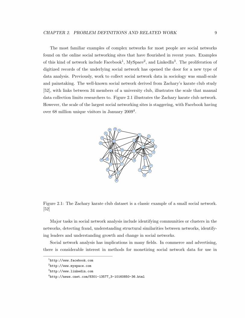
and painstaking. The well-known social network derived from Zachary’s karate club study
[52], with links between 34 members of a university club, illustrates the scale that manual
data collection limits researchers to. Figure 2.1 illustrates the Zachary karate club network.
However, the scale of the largest social networking sites is staggering, with Facebook having
over 68 million unique visitors in January 20094.
0
1
2
3
4
56
7
8
9
10
11
12
13
14
15
16
17
18
19
20
21
22
23
24
25
26
27
28
29
30
31
32
33
Figure 2.1: The Zachary karate club dataset is a classic example of a small social network.[52]
Major tasks in social network analysis include identifying communities or clusters in the
networks, detecting fraud, understanding structural similarities between networks, identify-
ing leaders and understanding growth and change in social networks.
Social network analysis has implications in many fields. In commerce and advertising,
there is considerable interest in methods for monetizing social network data for use in
1http://www.facebook.com2http://www.myspace.com3http://www.linkedin.com4http://news.cnet.com/8301-13577_3-10160850-36.html
CHAPTER 2. PROBLEM DEFINITIONS AND RELATED WORK 10
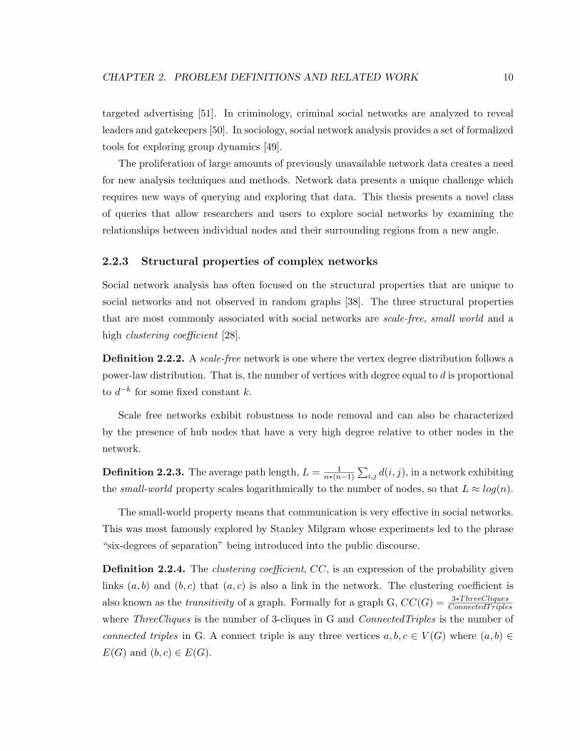
targeted advertising [51]. In criminology, criminal social networks are analyzed to reveal
leaders and gatekeepers [50]. In sociology, social network analysis provides a set of formalized
tools for exploring group dynamics [49].
The proliferation of large amounts of previously unavailable network data creates a need
for new analysis techniques and methods. Network data presents a unique challenge which
requires new ways of querying and exploring that data. This thesis presents a novel class
of queries that allow researchers and users to explore social networks by examining the
relationships between individual nodes and their surrounding regions from a new angle.
2.2.3 Structural properties of complex networks
Social network analysis has often focused on the structural properties that are unique to
social networks and not observed in random graphs [38]. The three structural properties
that are most commonly associated with social networks are scale-free, small world and a
high clustering coefficient [28].
Definition 2.2.2. A scale-free network is one where the vertex degree distribution follows a
power-law distribution. That is, the number of vertices with degree equal to d is proportional
to d−k for some fixed constant k.
Scale free networks exhibit robustness to node removal and can also be characterized
by the presence of hub nodes that have a very high degree relative to other nodes in the
network.
Definition 2.2.3. The average path length, L = 1n∗(n−1)
∑i,j d(i, j), in a network exhibiting
the small-world property scales logarithmically to the number of nodes, so that L ≈ log(n).
The small-world property means that communication is very effective in social networks.
This was most famously explored by Stanley Milgram whose experiments led to the phrase
“six-degrees of separation” being introduced into the public discourse.
Definition 2.2.4. The clustering coefficient, CC, is an expression of the probability given
links (a, b) and (b, c) that (a, c) is also a link in the network. The clustering coefficient is
also known as the transitivity of a graph. Formally for a graph G, CC(G) = 3∗ThreeCliquesConnectedTriples
where ThreeCliques is the number of 3-cliques in G and ConnectedTriples is the number of
connected triples in G. A connect triple is any three vertices a, b, c ∈ V (G) where (a, b) ∈E(G) and (b, c) ∈ E(G).
CHAPTER 2. PROBLEM DEFINITIONS AND RELATED WORK 11
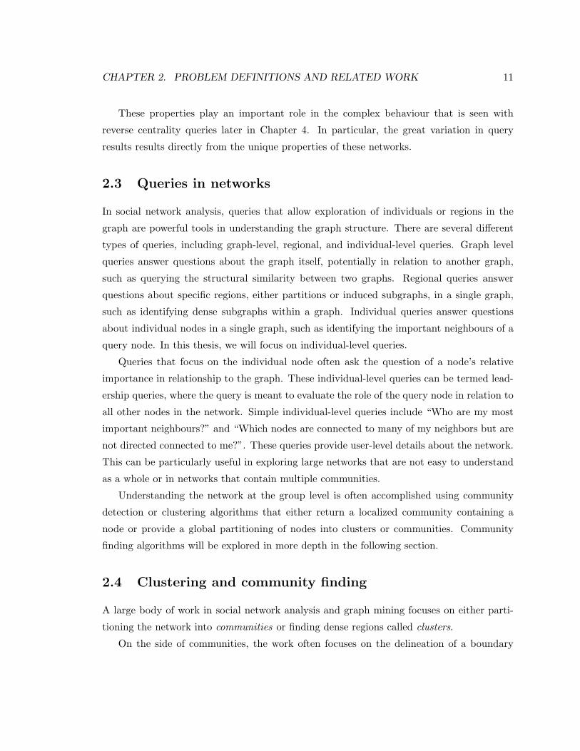
These properties play an important role in the complex behaviour that is seen with
reverse centrality queries later in Chapter 4. In particular, the great variation in query
results results directly from the unique properties of these networks.
2.3 Queries in networks
In social network analysis, queries that allow exploration of individuals or regions in the
graph are powerful tools in understanding the graph structure. There are several different
types of queries, including graph-level, regional, and individual-level queries. Graph level
queries answer questions about the graph itself, potentially in relation to another graph,
such as querying the structural similarity between two graphs. Regional queries answer
questions about specific regions, either partitions or induced subgraphs, in a single graph,
such as identifying dense subgraphs within a graph. Individual queries answer questions
about individual nodes in a single graph, such as identifying the important neighbours of a
query node. In this thesis, we will focus on individual-level queries.
Queries that focus on the individual node often ask the question of a node’s relative
importance in relationship to the graph. These individual-level queries can be termed lead-
ership queries, where the query is meant to evaluate the role of the query node in relation to
all other nodes in the network. Simple individual-level queries include “Who are my most
important neighbours?” and “Which nodes are connected to many of my neighbors but are
not directed connected to me?”. These queries provide user-level details about the network.
This can be particularly useful in exploring large networks that are not easy to understand
as a whole or in networks that contain multiple communities.
Understanding the network at the group level is often accomplished using community
detection or clustering algorithms that either return a localized community containing a
node or provide a global partitioning of nodes into clusters or communities. Community
finding algorithms will be explored in more depth in the following section.
2.4 Clustering and community finding
A large body of work in social network analysis and graph mining focuses on either parti-
tioning the network into communities or finding dense regions called clusters.
On the side of communities, the work often focuses on the delineation of a boundary
CHAPTER 2. PROBLEM DEFINITIONS AND RELATED WORK 12
between one community and another, with or without regard to the internal link structure.
Newman [39] defines a community as a subset of nodes which have more internal links
amongst themselves than external links extending from one of the member nodes to an
external node. This definition of community can be neatly quantified using Newman’s mea-
sure of modularity. A formal definition of modularity is given in Definition 2.1.5. Using
the modularity score as the objective function for an agglomerative clustering method pro-
vides a parameter free method for discovering the intrinsic community structure within a
graph, and as a method, will produce a graph partition that breaks down the graph into
non-overlapping communities.
Flake et al [18] use a network-flow approach to extract a local community that surrounds
a seed query. By using artificial links, the community threshold can be changed to produce
communities of varying size and cohesiveness. This work focuses on the directed web graph
and includes several examples of communities found using the algorithm.
Other work, such as that by Backstrom et al. [2], focuses on analyzing explicit commu-
nity growth where users self-identify with a group, rather than a community as commonly
defined by other authors. In particular, Backstrom et al. [2] focuses on identifying struc-
tural characteristics that make it likely that a user will join a group as well as the growth
and change in group membership over time.
Gibson et al. [21] focus on the heuristic extraction of dense subgraphs of a very large
graph. This technique has applications, in particular, for web graph analysis. No strict
definition of a community or cluster is defined here; rather a loose definition of a dense
bipartite subgraph exists where most of the links of the corresponding bipartite clique exist.
This method finds regions of the graph that are densely intra-connected, however, it does
not partition the graph nor does it find a localized community.
Recent work by Mishra et al. [36] has approached the clustering problem in a manner
which allows for overlapping communities to be found. This method finds induced subgraphs
where the separation between internal density and external sparsity is sufficient to meet
a fixed parameter. Colibri by Tong et al. [47] is another method that provides cluster
detection via a low rank approximation of the adjacency matrix.
Van Dongen [48] presents the Markov Cluster Algorithm (MCA) that is based on sim-
ulated flow across the network. This is achieved by simulating random walks across the
networks through iterative application of mathematical operators to the Markov matrix
representing the graph. MCA is useful in providing a fast clustering method that works well
CHAPTER 2. PROBLEM DEFINITIONS AND RELATED WORK 13
on large datasets with a small set of explicit parameters and no notion of a seed set.
There are a wide variety of community finding algorithms, with no clear favorite. Each
method has strengths and drawbacks but all share a common focus on the graph at large
and in that sense, may be considered graph-level queries.
The social network analysis community has also tackled the problem of modeling and
understanding the underlying processes in community formation, growth, and evolution.
Backstrom et al. [2] provide a through experimental analysis of communities in the dynamic
DBLP and LiveJournal datasets. At the node level they analyze the properties that influence
a node’s probability of joining a community, and at the group level they analyze the merging
of communities and movement in community interest is explored.
The relationship between community finding and the reverse centrality query is that they
provide two different approaches for identifying regions within graphs. Community finding
finds regions defined by their boundaries and internal link density. Reverse centrality queries
find regions centered on a query node where all nodes are dominated by the query node.
2.4.1 Related work on node queries
Kempe et al.’s work [29] on maximizing the spread of influence through a social network
is somewhat related to the reverse centrality query. The goal is to identify the most in-
fluential individuals in a social network using a model network that has directed, weighted
edges representing the level of influence one individual has over another together with some
threshold associated with each node. The most influential members in a network may be
akin to the nodes found to have large region of dominance by the reverse centrality queries
introduced later in this chapter. However, the reverse centrality queries do not rely on
specifically weighted edges and can be directly applied to only a subgraph. In addition, the
focus of the reverse centrality query is for a given node, identify a region, whereas Kempe
et al. focus on, for a given graph, identifying a node or set of nodes.
In addition, there are standard individual queries that are used in exploring the region
surrounding a query node. The most prominent of these queries is the k-neighborhood
query that returns all nodes reachable within a distance of k of the query node. This query
provides no guarantees on relationship between the query node and the result region other
than this distance guarantee.
CHAPTER 2. PROBLEM DEFINITIONS AND RELATED WORK 14
2.5 Centrality indices
Various centrality indices have been introduced in the past half century to explain the
relative importance of individuals in social networks. Centrality measures attempt to quan-
titatively capture the relative importance of the individual in relation to the group. There
are many measures of centrality including: degree centrality [38], betweenness centrality
[19], closeness centrality [41], bridging centrality [25], and Eigenvector centrality [6].
Centrality indices can be categorized based on the information used to calculate their
scores. There are three broad categories including vertex-based, distance-based, and path-
based centralities.
Discussion here is limited to centrality indices for vertices, although many naturally
extend to centrality indices for edges as well.
2.5.1 Degree-based centrality indices
Centrality indices based on degree include both the simple concept of degree centrality as
well as more sophisticated indices like PageRank [9] and HITS [31].
Definition 2.5.1. Degree centrality for a node v is defined as the number of links connecting
that node to other nodes in the graph G. Degree centrality, also known as vertex centrality
[38], can be expressed as:
CD(v) =degreeG(v)
n− 1(2.2)
A node with the highest degree centrality in a graph has the maximal number of neighbors
in the graph.
The idea of degree centrality is closely related to the idea of popularity in social net-
works, which is often measured informally as the number of links, or direct connections, an
individual has within the network.
More sophisticated measures are possible when graphs are directed, with both in-degree
and out-degree being considered. For the extent of this work, only undirected networks are
considered, and so the most relevant centrality index is degree centrality.
A family of degree-based centrality measures is described by Bonacich [6], where a pa-
rameter β determines the weighting of local versus global structure and a scaling parameter
α normalizes the score. His centrality formula is given as C(α, β) = α(I − βA)−1(A ∗ 1),where I is the identity matrix, A is the graph adjacency matrix, and 1 is a matrix of ones.
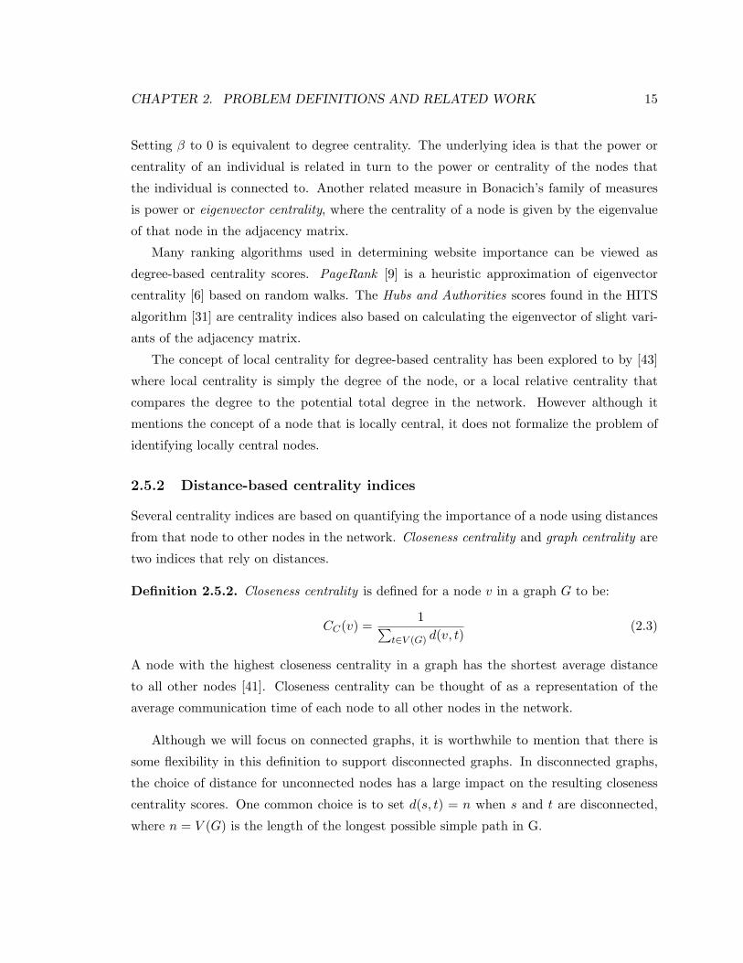
CHAPTER 2. PROBLEM DEFINITIONS AND RELATED WORK 15
Setting β to 0 is equivalent to degree centrality. The underlying idea is that the power or
centrality of an individual is related in turn to the power or centrality of the nodes that
the individual is connected to. Another related measure in Bonacich’s family of measures
is power or eigenvector centrality, where the centrality of a node is given by the eigenvalue
of that node in the adjacency matrix.
Many ranking algorithms used in determining website importance can be viewed as
degree-based centrality scores. PageRank [9] is a heuristic approximation of eigenvector
centrality [6] based on random walks. The Hubs and Authorities scores found in the HITS
algorithm [31] are centrality indices also based on calculating the eigenvector of slight vari-
ants of the adjacency matrix.
The concept of local centrality for degree-based centrality has been explored to by [43]
where local centrality is simply the degree of the node, or a local relative centrality that
compares the degree to the potential total degree in the network. However although it
mentions the concept of a node that is locally central, it does not formalize the problem of
identifying locally central nodes.
2.5.2 Distance-based centrality indices
Several centrality indices are based on quantifying the importance of a node using distances
from that node to other nodes in the network. Closeness centrality and graph centrality are
two indices that rely on distances.
Definition 2.5.2. Closeness centrality is defined for a node v in a graph G to be:
CC(v) =1∑
t∈V (G) d(v, t)(2.3)
A node with the highest closeness centrality in a graph has the shortest average distance
to all other nodes [41]. Closeness centrality can be thought of as a representation of the
average communication time of each node to all other nodes in the network.
Although we will focus on connected graphs, it is worthwhile to mention that there is
some flexibility in this definition to support disconnected graphs. In disconnected graphs,
the choice of distance for unconnected nodes has a large impact on the resulting closeness
centrality scores. One common choice is to set d(s, t) = n when s and t are disconnected,
where n = V (G) is the length of the longest possible simple path in G.
CHAPTER 2. PROBLEM DEFINITIONS AND RELATED WORK 16
Latora and Marchiori [34] present a measure termed efficiency that is based on the
mean distance between any two vertices in a network. The graph efficiency is very similar
to closeness centrality, as it is the inverse of closeness centrality, CC , divided by the number
of nodes in the graph. Closeness centrality and efficiency are most meaningful in connected
graphs.
Definition 2.5.3. Graph centrality is defined for a node v in a graph G to be:
CG(v) =1
maxt∈V (G) d(v, t)(2.4)
A node with the highest graph centrality in a graph has the shortest worst-case distance in
the graph [23].
Definition 2.5.4. The eccentricity Ev of a vertex v is defined as Ev = maxu∈G(dist(u, v)) .
A vertex v where Ev = minu∈G(Eu) is called a graph center for G. The minimum eccentricity
of a graph is called the radius of the graph.
Graph centrality is closely related to the graph theory concept of graph centers, which
are defined as the nodes in a graph with minimum eccentricity , where eccentricity is defined
as the longest shortest path to another node in the graph. The concepts of graph centers
and graph centrality itself are only meaningful in connected graphs, since in a disconnected
graph, all nodes would have the same graph centrality.
Distance-based centrality indices require calculation of all-pairs shortest paths (APSP)
to determine the distance matrix. The methods for APSP are explored in detail in Appendix
1.
Definition 2.5.5. Given a graph G = (V,E), the distance matrix D contains the pairwise
distances for all nodes in the graph, where each entry D[i, j] is equal to the distance between
nodes i, j ∈ G. The distance matrix is calculated by an APSP algorithm.
In distance matrix terms, the closeness centrality of a graph vertex is the inverse of the
sum of the row representing the vertex. The graph centrality is the inverse of the maximum
value in the row representing the vertex.
2.5.3 Path-based centrality indices
Path-based centrality indices are those measures that rely on calculating explicit shortest
path information about the graph. Unlike distance-based centrality indices, where the
CHAPTER 2. PROBLEM DEFINITIONS AND RELATED WORK 17
distance matrix is required for computation, path-based indices require explicit knowledge
of what nodes are involved in which shortest paths.
Definition 2.5.6. Betweenness centrality BCv for a node v is defined as
CCv =∑
t=u=v∈G(ηtu(v)/ηtu) (2.5)
Where ηtu(v) is the number of shortest paths between t and u that include v and ηtu is the
total number of shortest paths between t and u. Betweenness centrality is the fraction of
all shortest paths that pass through the node v [19].
Betweenness centrality is an expensive index to calculate for large graphs. Before Bran-
des [7] introduced an algorithm with O(nm) time complexity and O(n+m) space complexity,
the best known algorithm had cubic time complexity. In the naıve implementation, storage of
all shortest path representations could be within the order of O(n3). Various approximation
methods have been suggested for betweenness centrality, including variants on betweenness
that are easier to calculate [38]. Betweenness centrality is distinct from other centrality
indices discussed here because a node of high betweenness centrality does not necessarily
indicate that the node is an important node in the graph. A node of high betweenness
means that upon deletion, the shortest paths of the network are heavily affected.
Beyond betweenness centrality, other path-based centrality indices have been defined
including stress centrality [45], which is an absolute count of the number of shortest paths
that the node participates in.
Due to the complexity in calculating and maintaining all shortest paths in an incremental
fashion, we will not explore path-based centrality variants of reverse centrality queries in
this thesis.
CHAPTER 2. PROBLEM DEFINITIONS AND RELATED WORK 18
2.6 Problem definitions
In this section, we give a general problem definition for the reverse centrality query, the
novel query introduced by this thesis. More detailed problem definitions are provided for
individual reverse centrality query types that are described and explored further in this
thesis.
2.6.1 Reverse centrality queries
The novel class of queries called reverse centrality queries are leadership queries, where an
individual node is evaluated in terms of some centrality index, but where the result is in
terms of a region where the node dominates. This class of queries ties together the idea of
global centrality measures with that of local behavior of a query node.
The query result is a region, an induced subgraph, where the query point is a local
leader. There are potentially an exponential number of results if the query node q globally
dominates every subgraph which contains it. In order to reduce the size of the potential
answer, a single result is returned. The result is a locally optimal choice according to the
search algorithm.
2.6.2 Local centrality dominance
Reverse centrality queries seek to find an induced subgraph surrounding a query vertex that
is dominated by that query vertex.
Definition 2.6.1. A query vertex q ∈ G dominates the connected induced subgraph S ⊆ G
if and only if q ∈ S and ∀v ∈ S, centralityS(q) ≥ centralityS(v). That is, for some centrality
measure, centralityS , calculated over the induced subgraph S, the vertex q has maximal
centrality. We may also refer to q as locally dominant in S. A vertex q is called globally
dominant if it dominates G.
Notice that the dominance defined in Definition 2.6.1 is not strict. There may be other
nodes in the subgraph S that are equally dominant with q. This looser definition is used to
allow for the many real world cases of symmetry where two or more nodes will share similar
or identical local structure.
Definition 2.6.2. A maximally dominant induced subgraph is dominated by the query
node q, where for all induced subgraphs with V (A)∪V (S) where V (A) is some set of nodes
CHAPTER 2. PROBLEM DEFINITIONS AND RELATED WORK 19
in V (G)\V (S), q does not dominate. In other words, no larger induced subgraph containing
the nodes in V (S) is dominated by q.
Definition 2.6.3. A 1-maximally dominant induced subgraph S is dominated by the query
vertex q, but ∀u ∈ S, v /∈ S, (u, v) ∈ E(G), the induced subgraph v ∪ S is not dominated
by q. This means that no single node may be added to S such that we obtain a larger
connected induced subgraph where q dominates. These subgraphs may also be referred to
as locally optimal subgraphs.
To limit the size of the query answer, results are limited to those called maximally domi-
nant. In addition, it is only meaningful to explore the space of connected induced subgraphs,
as the centrality measures are most meaningful when applied to connected graphs.
The definition of maximally dominant induced subgraphs corresponds to the notion of
a local maximum. Where 1-maximally dominant regions correspond to a local maximum
where no single neighbour of the induced subgraph S not yet in S can be added to S while
keeping q as a dominant node.
Definition 2.6.4. A locally central node q is a node that dominates, according to a cen-
trality measure, an induced subgraph H of the graph G where q ∈ V (H).
Definition 2.6.5. A local centrality measure is a theoretical measure that would provide a
means of quantifying the behaviour of a node q according to some centrality measure C in
induced subgraphs containing q. A node with high local centrality would be locally central
to a relatively large region, whereas a node with low local centrality would remain peripheral
even in induced subgraphs.
In Chapter 4, we use the size of the query result of a reverse centrality query as a proxy
for the local centrality of each node.
2.6.3 Reverse degree centrality query
The reverse degree centrality problem returns an induced subgraph S where the query node
q has a degree equal to the maximum degree observed in the subgraph S.
Definition 2.6.6. The reverse degree centrality query on a query node q returns a connected
induced subgraph S that is dominated by q. In the induced subgraph S, q has maximal
degree. In addition, we restrict S to be maximally dominant.
CHAPTER 2. PROBLEM DEFINITIONS AND RELATED WORK 20
The degree centrality index itself is relatively simple, being given by the degree of the
vertex, yet is still non-trivial when applied to finding a dominated subset that satisfied the
reverse degree centrality query. Determining whether an induced subgraph is dominated
by the query vertex is non-trivial because the degree of a vertex v in an induced subgraph
depends on the number of neighbours of that are members of the induced subgraph, thus
the degree centrality of nodes will change as additional nodes are added to the region.
Degree centrality neighbourhood dominance query
This section provides a constrained version of the general reverse centrality query. This
definition may prove useful for exploring the physical distribution of vertex degree within
a graph. This query is not explored further here, but this query provides an example of
an extension that integrates well with the existing study of complex networks in terms of
degree distribution.
Definition 2.6.7. The degree centrality neighbourhood dominance query returns the dis-
tance, d, to the nearest node which dominates q with respect to the graph G. The (d− 1)−neighbourhood contains all nodes closer than d to q and therefore the (d−1)−neighbourhoodmust be dominated by q.
The neighbourhood dominance query is a special constraint on the general reverse de-
gree centrality query, where the returned set S must contain exactly the largest complete
neighbourhood graph of q where q dominates.
Applications of reverse degree centrality
Degree centrality identifies nodes with high degree as central, as a result the centrality
measure relies on an assumption that nodes with many connections are more important
than those on the periphery. Degree centrality defines prominent nodes to be nodes with
many connections [49].
The reverse degree centrality problem then provides a region over which the query node q
is prominent by this definition. In many social network contexts, popularity is equated with
the number of friends, or relationships, an individual has. The reverse degree centrality
query would allow a user to determine a group of people (which may be considered a
community or social group) in which they are the most popular (or tied for most popular)
individual, as determined by node degree.
CHAPTER 2. PROBLEM DEFINITIONS AND RELATED WORK 21
In the context of complex networks representing businesses as nodes and client relation-
ships between businesses as links, the reverse degree centrality query may also prove useful.
The query result for a queried business would result a group of businesses within which
the queried business has the most connections (or a tie for most) within that group. If the
extension for weighted edges is used and weight is used to represent sales volume, the query
result becomes a group of connected businesses where the queried business has the highest
sales volume.
2.6.4 Reverse closeness centrality query
The reverse closeness centrality query returns a locally maximal induced subgraph where
the query vertex q has the minimal average distance to the rest of the induced subgraph.
Definition 2.6.8. The reverse closeness centrality query on a query node q returns a con-
nected induced subgraph S that is dominated by q according to closeness centrality. In the
induced subgraph S, q has minimal mean distance to other nodes in the graph. In addition,
we restrict S to be maximally dominant.
The reverse closeness centrality query can be applied to communication networks. In
this application, the reverse closeness query calculates, with respect to a query node q, an
induced subgraph surrounding q where q has minimal mean distance to all other nodes. In
this context, q would be a good choice as a leader node over S in a communication protocol
that requires that messages be sent to a leader for redistribution.
The reverse closeness centrality query result is a connected induced subgraph centered
on q, where the center is defined by average distance to all other nodes. This corresponds
somewhat to the facility location problem using an optimizing function of average distance.
[8]
The definition of closeness centrality used here could be easily expanded to handle
weighted graphs, where edges have weights associated with them by modifying the dis-
tance used in the definition to be the sum of edge weights rather than the number of edges
in the shortest path.
Applications of reverse closeness centrality queries
The reverse closeness centrality query provides a practical network analysis tool in several
different contexts.
CHAPTER 2. PROBLEM DEFINITIONS AND RELATED WORK 22
In the context of communication networks, the returned region provides a subgraph over
which the query node q is a suitable candidate for a leader, where a leader should minimize
round-trip communication costs to all other nodes.
In the context of social networks, the returned region represents a group of individuals
where the query node q plays a central role: they are, the closest node, on average, to the
rest of the graph. The resulting region could be used to provide a meaningful cluster of
individuals centered on the query node. This result could provide an innovative interface
for individuals exploring their own social networks from a user’s perspective. Rather than
showing friends and friends of friends, this region may contain those connected at greater
distance, but still those who are well connected to the individual.
2.6.5 Reverse graph centrality query
Hage and Harary [23] originally defined the problem of graph centrality, a centrality measure
based on the graph theory notion of a graph center. The reverse graph centrality query seeks
induced subgraphs where the query vertex q has the best worst-case distance to any other
node. In other words, where q is a graph center.
Definition 2.6.9. The reverse graph centrality query on a query node q returns a connected
induced subgraph S that is dominated by q according to graph centrality. In the induced
subgraph S, q has minimal worst-case distance to other nodes in the graph. In addition, we
restrict S to be maximally dominant.
An induced subgraph where the query point q is a vertex center will be centered about
q. Using the graph centrality criterion, an induced subgraph S is dominated by the query
point q if and only if q is a graph center of S.
Applications of reverse graph centrality queries
In the application of social networks, the result of a reverse graph centrality query on a query
node q would return the induced subgraph S of individuals over which q is most central,
where a central individual has fewest maximum hops required to reach anyone else in S.
Graph center-based approaches for energy efficient communication protocols on wireless
sensor networks as described in [35] show the applicability of graph centers to a real world
problem.
CHAPTER 2. PROBLEM DEFINITIONS AND RELATED WORK 23
By enabling the extraction of the cluster that forms around a single vertex (the query
vertex), the user is able to explore the area of local dominance for the query vertex.
The reverse graph centrality region represents a centered region around the query node
where the query node is the graph center. This centered region will not include other nodes
that are more prominent than the query node and in that sense will focus on the area of
dominance for the query node.
This type of query would be useful for social network exploration, allowing individuals
to explore their social connections in a fashion the focuses on those they are most closely
connected to. Given the small world property of social networks, providing the neighborhood
(those who are perhaps 2, 3 or 4 links away from an individual) would prove to be an
increasingly unwieldy region. Rather than multiple neighbourhood queries, we return a
centered region using a parameter free method and that is guaranteed to be centered on the
node.
2.6.6 Constrained queries
Extensions to the problem definitions for reverse centrality queries can be made by placing
additional constraints on the desired answer. Constraints include inclusion and exclusion of
other nodes in the result, and constraints on the size of the desired induced subgraph.
Although these definitions are not explored further within this thesis, the formalization
of these variants may prove useful. We provide these definitions because they are the most
natural extensions to the reverse centrality queries defined above. Algorithmic modifications
to implement these constraints would be fairly simple, but the analysis of these constraints
is best left to a dataset-specific study.
Follower constraints
Follower constraints place additional constraints on the induced subgraph result for a reverse
centrality query by requiring either the inclusion or exclusion of nodes other than q from
the result S.
Definition 2.6.10. Let F be a set containing one or more nodes in G. For a reverse
centrality query with query node q and the resulting induced subgraph S, a follower inclusion
constraint requires that F ⊆ V (S), so S must contain the followers in F . Similarly, a follower
exclusion constraint requires that V (S) ∩ F = ∅, so S contains none of the followers in F .

CHAPTER 2. PROBLEM DEFINITIONS AND RELATED WORK 24
Follower constraints provide more opportunity for the user to modify the potential query
result and also help the user to intuitively explore the space of potential induced subgraph
results. These constraints also allow the user to answer queries of the form, “In what group,
as defined by an induced subgraph, is q the leader, but s the follower?”.
Neighbourhood constraints
In very large graphs, neighborhood constraints may improve speed by isolating the search
space to a smaller graph.
Definition 2.6.11. For a reverse centrality query with query node q and the resulting
induced subgraph S, a neighbourhood constraint requires that S only includes nodes within
a specified distance of q, or in other words, within the k-neighbourhood of q, where k is a
fixed parameter, k > 0.
Neighbourhood size constraints allow for quicker result calculation and may be used to
help the user gauge the importance of a node locally without potentially returning an in-
duced subgraph equal to the entire graph, which is possible if q were also globally dominant.
Chapter 3
Reverse Centrality Queries:
Algorithms
The algorithms presented in this chapter are methods for finding locally optimal solutions
to reverse centrality queries. We naturally approach these problems using a breadth first
search method to incrementally add nodes until a local maximum is reached. The query
results are locally optimal subgraphs, as defined in Definition 2.6.3, where no neighbor node
of the current subgraph could be added to produce a larger induced subgraph dominated
by the query point q.
One limitation of these algorithms is that they are all input dependent, they will possibly
produce different answers if the dataset is permuted. As defined now, they will produce one
locally maximal induced subgraph in response to a query. This could be expanded to allow
k randomized trials to potentially produce up to k different answers. From the randomized
trials, the largest result could be returned.
For any reverse centrality query, one trivial answer is always available. For the induced
subgraph defined by V (S) = {q} where q is the query node, it follows trivially that q is the
leader of the induced subgraph S. This means that in the most basic case, we will always
have a query result. Although, as we prove later in this chapter, we can guarantee that the
query result will be more than just q.
Detailed algorithms for the reverse closeness, graph and degree centrality queries are
presented. For each query type, proofs are given for basic properties of the algorithm. In
addition, heuristic optimizations for each of the algorithms presented are provided.
25
CHAPTER 3. REVERSE CENTRALITY QUERIES: ALGORITHMS 26
Justification for returning a single region
The problem of finding all induced subgraphs in G where the query node q is a dominating
node is a very challenging problem due to the potentially exponential number of induced
subgraphs satisfying this condition. For a given induced subgraph, the method for deter-
mining whether the query node q is a dominating node is polynomial. However, the size of
the output for this problem is potentially exponential in terms of the size of the input.
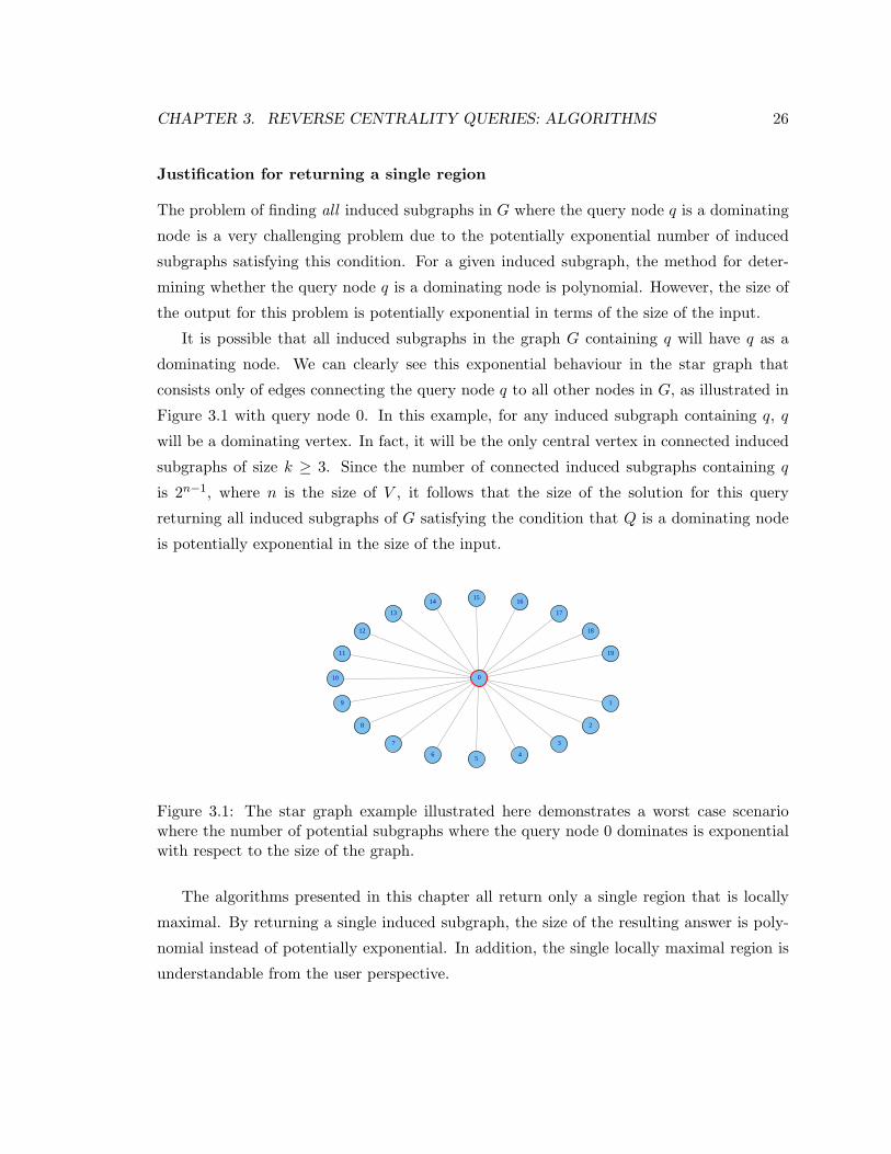
It is possible that all induced subgraphs in the graph G containing q will have q as a
dominating node. We can clearly see this exponential behaviour in the star graph that
consists only of edges connecting the query node q to all other nodes in G, as illustrated in
Figure 3.1 with query node 0. In this example, for any induced subgraph containing q, q
will be a dominating vertex. In fact, it will be the only central vertex in connected induced
subgraphs of size k ≥ 3. Since the number of connected induced subgraphs containing q
is 2n−1, where n is the size of V , it follows that the size of the solution for this query
returning all induced subgraphs of G satisfying the condition that Q is a dominating node
is potentially exponential in the size of the input.
0
1
2
3
45
6
7
8
9
10
11
12
13
1415
16
17
18
19
Figure 3.1: The star graph example illustrated here demonstrates a worst case scenariowhere the number of potential subgraphs where the query node 0 dominates is exponentialwith respect to the size of the graph.
The algorithms presented in this chapter all return only a single region that is locally
maximal. By returning a single induced subgraph, the size of the resulting answer is poly-
nomial instead of potentially exponential. In addition, the single locally maximal region is
understandable from the user perspective.
CHAPTER 3. REVERSE CENTRALITY QUERIES: ALGORITHMS 27
Optimality of Result
We are unable to guarantee a globally optimal query result due to the difficulty of the reverse
centrality query problem. A globally optimal result may be defined as the largest possible
region containing q that is dominated by q, where size is determined by the number of nodes
in the region.
In Chapter 2, the problem definitions given for the reverse centrality queries are based
on the idea of maximally dominant regions. While theoretically this would be a high quality
result to return, it would be prohibitively expensive to satisfy this definition algorithmically.
For practical purposes, we will provide algorithms that find a 1-maximally dominant
induced subgraph as the search space of ensuring that all supergraphs of S are not dominated
is potentially exponential. By this definition, no single node in the one-neighbourhood of S
can be successfully added to S while maintaining q as the dominant node.
3.1 Reverse degree centrality query
The reverse degree centrality query provides an induced subgraph, or region, where the
query node dominates according to degree centrality. In terms of a social network, this
means that the query returns a group of individuals within which the query individual has
the greatest number of relationships within that group compared to other members of the
group.
Degree centrality differs from the other centralities explored for reverse centrality queries
in that it is a degree-based centrality index that relies only on local information.
The static degree centrality algorithm is trivial, as the vertex degree of each node in the
global graph is either known (in graph representations where edges are stored with respect
to each vertex) or easy to calculate (in graph representations with separate edge lists). With
knowledge of the degree of each node, the ordered list that determines the ranking according
to degree centrality can be established in O(n logn) time.
As is explored in greater detail in the following sections, it is easy to construct a fast
incremental algorithm to produce a reverse degree centrality query answer for a given query
node.
CHAPTER 3. REVERSE CENTRALITY QUERIES: ALGORITHMS 28
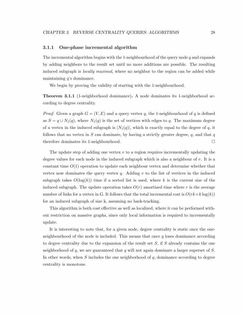
3.1.1 One-phase incremental algorithm
The incremental algorithm begins with the 1-neighbourhood of the query node q and expands
by adding neighbors to the result set until no more additions are possible. The resulting
induced subgraph is locally maximal, where no neighbor to the region can be added while
maintaining q’s dominance.
We begin by proving the validity of starting with the 1-neighbourhood.
Theorem 3.1.1 (1-neighborhood dominance). A node dominates its 1-neighborhood ac-
cording to degree centrality.
Proof. Given a graph G = (V,E) and a query vertex q, the 1-neighbourhood of q is defined
as S = q ∪N1(q), where N1(q) is the set of vertices with edges to q. The maximum degree
of a vertex in the induced subgraph is |N1(q)|, which is exactly equal to the degree of q, it
follows that no vertex in S can dominate, by having a strictly greater degree, q, and that q
therefore dominates its 1-neighbourhood.
The update step of adding one vertex v to a region requires incrementally updating the
degree values for each node in the induced subgraph which is also a neighbour of v. It is a
constant time O(1) operation to update each neighbour vertex and determine whether that
vertex now dominates the query vertex q. Adding v to the list of vertices in the induced
subgraph takes O(log(k)) time if a sorted list is used, where k is the current size of the
induced subgraph. The update operation takes O(r) amortized time where r is the average
number of links for a vertex in G. It follows that the total incremental cost is O(rk+k log(k))
for an induced subgraph of size k, assuming no back-tracking.
This algorithm is both cost effective as well as localized, where it can be performed with-
out restriction on massive graphs, since only local information is required to incrementally
update.
It is interesting to note that, for a given node, degree centrality is static once the one-
neighbourhood of the node is included. This means that once q loses dominance according
to degree centrality due to the expansion of the result set S, if S already contains the one
neighborhood of q, we are guaranteed that q will not again dominate a larger superset of S.
In other words, when S includes the one neighborhood of q, dominance according to degree
centrality is monotone.
CHAPTER 3. REVERSE CENTRALITY QUERIES: ALGORITHMS 29
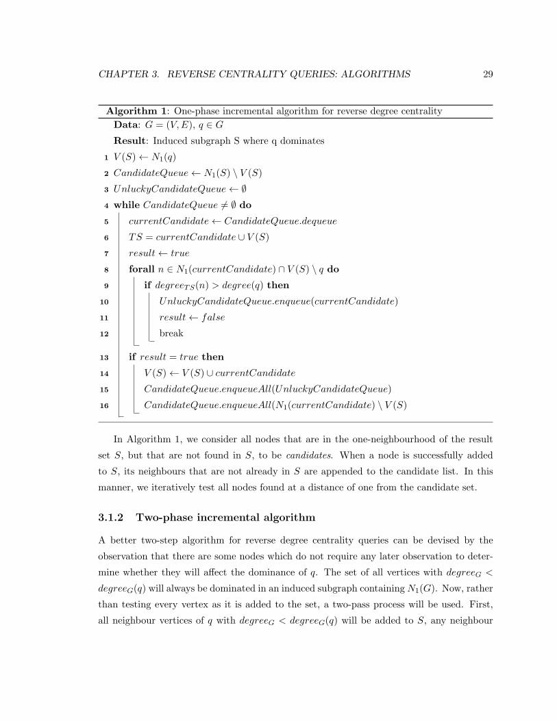
Algorithm 1: One-phase incremental algorithm for reverse degree centrality
Data: G = (V,E), q ∈ G
Result: Induced subgraph S where q dominates
V (S)← N1(q)1
CandidateQueue← N1(S) \ V (S)2
UnluckyCandidateQueue← ∅3
while CandidateQueue = ∅ do4
currentCandidate← CandidateQueue.dequeue5
TS = currentCandidate ∪ V (S)6
result← true7
forall n ∈ N1(currentCandidate) ∩ V (S) \ q do8
if degreeTS(n) > degree(q) then9
UnluckyCandidateQueue.enqueue(currentCandidate)10
result← false11
break12
if result = true then13
V (S)← V (S) ∪ currentCandidate14
CandidateQueue.enqueueAll(UnluckyCandidateQueue)15
CandidateQueue.enqueueAll(N1(currentCandidate) \ V (S)16
In Algorithm 1, we consider all nodes that are in the one-neighbourhood of the result
set S, but that are not found in S, to be candidates. When a node is successfully added
to S, its neighbours that are not already in S are appended to the candidate list. In this
manner, we iteratively test all nodes found at a distance of one from the candidate set.
3.1.2 Two-phase incremental algorithm
A better two-step algorithm for reverse degree centrality queries can be devised by the
observation that there are some nodes which do not require any later observation to deter-
mine whether they will affect the dominance of q. The set of all vertices with degreeG <
degreeG(q) will always be dominated in an induced subgraph containingN1(G). Now, rather
than testing every vertex as it is added to the set, a two-pass process will be used. First,
all neighbour vertices of q with degreeG < degreeG(q) will be added to S, any neighbour
CHAPTER 3. REVERSE CENTRALITY QUERIES: ALGORITHMS 30
vertices that do not meet this criterion will be added to the candidate list. The process will
continue recursively with the newly added vertices until the induced subgraph S contains
all vertices globally dominated by q with respect to G that are directly connected to q via
a path of other dominated vertices.
The second step is to go through the queue of candidate vertices that are not globally
dominated by q and to see which of these vertices can be added to S without challenging
the dominance of q, using the same testing procedures as the one-pass algorithm.
The neighbours of successfully added candidate vertices would be added to the back of
the queue if they are not already in S. The process would stop when no candidate can
be successfully added to S. This process is input-sensitive, in that a different ordering of
candidate nodes could produce a different set S when the algorithm finishes.
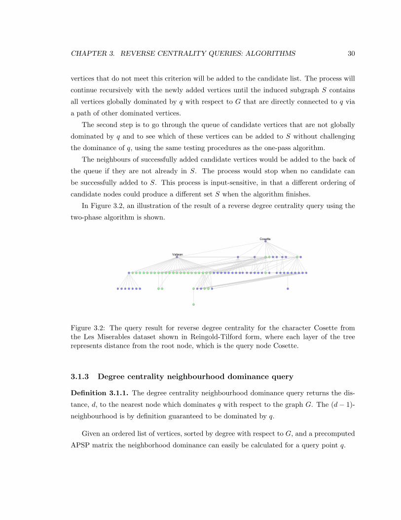
In Figure 3.2, an illustration of the result of a reverse degree centrality query using the
two-phase algorithm is shown.
Figure 3.2: The query result for reverse degree centrality for the character Cosette fromthe Les Miserables dataset shown in Reingold-Tilford form, where each layer of the treerepresents distance from the root node, which is the query node Cosette.
3.1.3 Degree centrality neighbourhood dominance query
Definition 3.1.1. The degree centrality neighbourhood dominance query returns the dis-
tance, d, to the nearest node which dominates q with respect to the graph G. The (d− 1)-
neighbourhood is by definition guaranteed to be dominated by q.
Given an ordered list of vertices, sorted by degree with respect to G, and a precomputed
APSP matrix the neighborhood dominance can easily be calculated for a query point q.
CHAPTER 3. REVERSE CENTRALITY QUERIES: ALGORITHMS 31
Starting from q, a breadth first search with a search criterion of degreeG(v) > degreeG(q)
will provide an answer to minimum distance, d, to a dominating node, since the first node
found is guaranteed to be as close as possible. The depth of the search at this point provides
the minimum distance to a dominating node. This search takes time O(r) where r is the
size of the d-neighbourhood of q. This is potentially expensive if q is the globally dominant
vertex, or dominates a large portion of the vertices in G.
Another approach is to look-up the distance of each vertex in the graph known to have a
higher degree than q. Assuming that all distances have been precomputed, this takes O(1)
time for each comparison, if it has not been precomputed, it will take one single-pair shortest
path (SPSP) calculation per node, or one single source shortest paths (SSSP) calculation
(whichever is more advantageous) to determine the distance between q and the vertex in
question. The node with a greater degree than q at minimum distance takes O(kp) where p
is the number of vertices in G with a greater degree and O(k) is the comparison time needed
to determine the distance from q to the vertex in question.
Experiments for this variant of the reverse degree centrality query are not provided in
Chapter 4, but are left for future experimentation.
3.2 Reverse closeness centrality query
The reverse closeness centrality query returns an induced subgraph (a region), where the
query node q has minimal average distance to all other nodes.
It is meaningful to explore the best available methods for closeness centrality in the
traditional whole graph. To implement an incremental algorithm for closeness centrality, we
will require a dynamic closeness centrality method that allows for the reuse of calculations
as the region grows.
For calculating closeness centrality in the static case, Brandes’ betweenness algorithm [7]
is immediately applicable to the closeness centrality measure as well. It provides a method
for calculating closeness centrality in O(n + m) space and O(nm) time where n is the
number of vertices and m is the number of edges. Brandes’ algorithm relies on a recursive
construction of shortest paths where explicit shortest paths are not stored. Unfortunately,
this means that it is not possible to modify Brandes’ algorithm to provide an incremental
algorithm that performs better than repeating the entire algorithm at each step.
Closeness centrality may also be calculated from the distance matrix of the graph G,
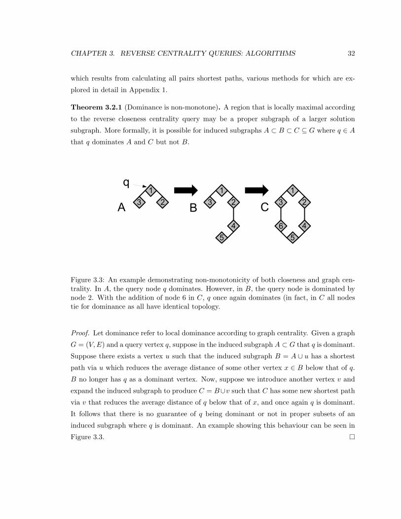
CHAPTER 3. REVERSE CENTRALITY QUERIES: ALGORITHMS 32
which results from calculating all pairs shortest paths, various methods for which are ex-
plored in detail in Appendix 1.
Theorem 3.2.1 (Dominance is non-monotone). A region that is locally maximal according
to the reverse closeness centrality query may be a proper subgraph of a larger solution
subgraph. More formally, it is possible for induced subgraphs A ⊂ B ⊂ C ⊆ G where q ∈ A
that q dominates A and C but not B.
Figure 3.3: An example demonstrating non-monotonicity of both closeness and graph cen-trality. In A, the query node q dominates. However, in B, the query node is dominated bynode 2. With the addition of node 6 in C, q once again dominates (in fact, in C all nodestie for dominance as all have identical topology.
Proof. Let dominance refer to local dominance according to graph centrality. Given a graph
G = (V,E) and a query vertex q, suppose in the induced subgraph A ⊂ G that q is dominant.
Suppose there exists a vertex u such that the induced subgraph B = A ∪ u has a shortest
path via u which reduces the average distance of some other vertex x ∈ B below that of q.
B no longer has q as a dominant vertex. Now, suppose we introduce another vertex v and
expand the induced subgraph to produce C = B∪v such that C has some new shortest path
via v that reduces the average distance of q below that of x, and once again q is dominant.
It follows that there is no guarantee of q being dominant or not in proper subsets of an
induced subgraph where q is dominant. An example showing this behaviour can be seen in
Figure 3.3.
CHAPTER 3. REVERSE CENTRALITY QUERIES: ALGORITHMS 33
The non-monotonicity of dominance for closeness centrality tells us that the incremental
algorithm can only promise to provide locally optimal results. We are not guaranteed to
find the largest possible region by this search process. This also indicates that an optimal
greedy algorithm or dynamic programming solution is not possible. In addition, even if we
start with a globally dominant node, we cannot guarantee that we will return the entire
graph G as the result, as the result may be sub-optimal even in this case.
While the proof that dominance is non-monotone does not prove the case for strict
dominance, where the query node is strictly better than any other node in S according
to the centrality measure, larger example graphs demonstrating strict dominance may be
constructed. Such examples take the general form where the query node q is central to two
large, balanced portions of the graph. When only one portion of the graph is contained in
S, q does not dominate, the second portion must be added before q again dominates.
Theorem 3.2.2 (1-neighborhood dominance). A node dominates its 1-neighborhood ac-
cording to closeness centrality.
Proof. Given a graph G = (V,E) and a query vertex q, the 1-neighbourhood of q is defined
as S = q ∪N1(q), an induced subgraph, where N1(q) is the set of vertices with edges to q.
The best closeness centrality achievable is to have an average distance of 1 to other vertices.
By definition, q has a distance of 1 to all neighbours. It follows that in S, q has optimal
closeness centrality and therefore cannot be dominated by any other vertex in S. Therefore,
q dominates its 1-neighbourhood.
Because a node always dominates its 1-neighbourhood, we can start the incremental
algorithm beginning with the 1 neighbourhood of the query node q.
3.2.1 Incremental algorithm
When adding a new vertex v to an induced subgraph S (or graph), only new shortest paths
via v will lead to decreased distances. It is this critical observation that we will use when
determining updates to the distance matrix in our algorithm.
In order to dynamically update our closeness centrality scores, it is necessary to know
the distance from the new vertex v to all other vertices in the graph. We can calculate
these distances by determining the single-source shortest paths (SSSP). There are many
known algorithms for calculating SSSP including Dijkstra’s algorithm. However, because
CHAPTER 3. REVERSE CENTRALITY QUERIES: ALGORITHMS 34
the current distance matrix has been stored for the region S, a full SSSP calculation is not
required to update the distance matrix for V (S) ∩ v. The distance to all neighbors of the
candidate node will be 1 and the distance of a node, v, that is not direct neighbour will be
defined by the minimum distance between a neighbour of the candidate node and v, since
all paths from the candidate node must pass through a neighbour of the candidate.
Once the shortest distances from v to all other vertices are known, this update algorithm,
in time O(k2) where k = |V (S)|, presented in Algorithm 3 can check whether any shortest
path via v is shorter than the existing path. This assumes that a shortest distance matrix is
being updated and stores explicitly all existing all-pairs distances in the graph. The average
distance for each vertex can be updated in O(1) time, for each change in a shortest path
that affects that vertex. The algorithm halts when no candidate vertices can be added to S
without losing q’s dominance.
In the pathological worst case, this algorithm can perform up to O(n2) candidate node
tests, with each test taking O(k2) time, leading to a worst case complexity of O(n4). This
only happens if the only possible successful candidate is always located at the end of the
candidate list and the returned region is equal to the entire graph. The space complexity in
all cases is O(k2) where k = |V (S)| due to the need to store the distance matrix. However,
in practice, average complexity is significantly better. Additionally, each distance matrix
update is independent, meaning that this portion of the operation could be multi-threaded
to greatly increase query speed in practice.
The algorithm is split into two blocks for formatting purposes due to the limitations
of typesetting algorithms. These two blocks together define the incremental algorithm for
reverse closeness centrality queries. The first block, given in Algorithm 2, contains the
initialization of all variables for S when S contains the 1-neighborhood of q. The second
block, given in Algorithm 3, defines the growth stage of the incremental algorithm.
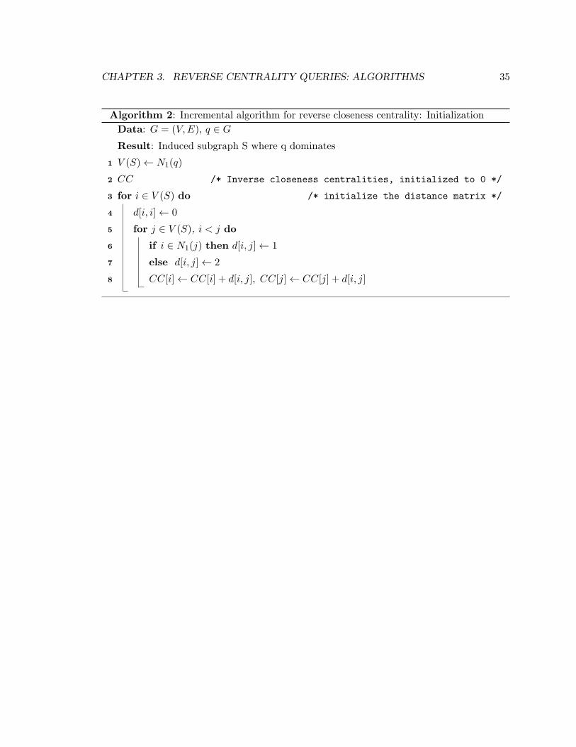
CHAPTER 3. REVERSE CENTRALITY QUERIES: ALGORITHMS 35
Algorithm 2: Incremental algorithm for reverse closeness centrality: Initialization
Data: G = (V,E), q ∈ G
Result: Induced subgraph S where q dominates
V (S)← N1(q)1
CC /* Inverse closeness centralities, initialized to 0 */2
for i ∈ V (S) do /* initialize the distance matrix */3
d[i, i]← 04
for j ∈ V (S), i < j do5
if i ∈ N1(j) then d[i, j]← 16
else d[i, j]← 27
CC[i]← CC[i] + d[i, j], CC[j]← CC[j] + d[i, j]8
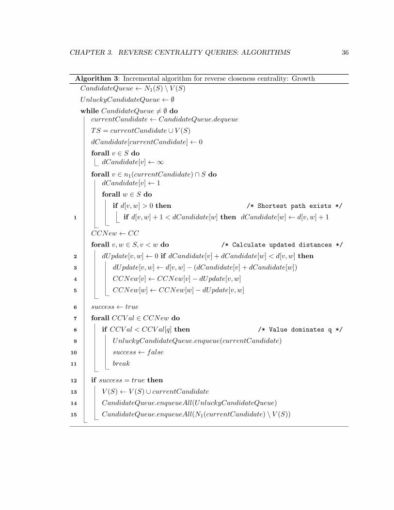
CHAPTER 3. REVERSE CENTRALITY QUERIES: ALGORITHMS 36
Algorithm 3: Incremental algorithm for reverse closeness centrality: Growth
CandidateQueue← N1(S) \ V (S)
UnluckyCandidateQueue← ∅while CandidateQueue = ∅ do
currentCandidate← CandidateQueue.dequeue
TS = currentCandidate ∪ V (S)
dCandidate[currentCandidate]← 0
forall v ∈ S dodCandidate[v]←∞
forall v ∈ n1(currentCandidate) ∩ S dodCandidate[v]← 1
forall w ∈ S do
if d[v, w] > 0 then /* Shortest path exists */
if d[v, w] + 1 < dCandidate[w] then dCandidate[w]← d[v, w] + 11
CCNew ← CC
forall v, w ∈ S, v < w do /* Calculate updated distances */
dUpdate[v, w]← 0 if dCandidate[v] + dCandidate[w] < d[v, w] then2
dUpdate[v, w]← d[v, w]− (dCandidate[v] + dCandidate[w])3
CCNew[v]← CCNew[v]− dUpdate[v, w]4
CCNew[w]← CCNew[w]− dUpdate[v, w]5
success← true6
forall CCV al ∈ CCNew do7
if CCV al < CCV al[q] then /* Value dominates q */8
UnluckyCandidateQueue.enqueue(currentCandidate)9
success← false10
break11
if success = true then12
V (S)← V (S) ∪ currentCandidate13
CandidateQueue.enqueueAll(UnluckyCandidateQueue)14
CandidateQueue.enqueueAll(N1(currentCandidate) \ V (S))15
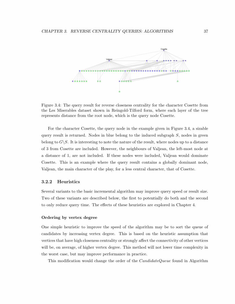
CHAPTER 3. REVERSE CENTRALITY QUERIES: ALGORITHMS 37
Figure 3.4: The query result for reverse closeness centrality for the character Cosette fromthe Les Miserables dataset shown in Reingold-Tilford form, where each layer of the treerepresents distance from the root node, which is the query node Cosette.
For the character Cosette, the query node in the example given in Figure 3.4, a sizable
query result is returned. Nodes in blue belong to the induced subgraph S, nodes in green
belong to G\S. It is interesting to note the nature of the result, where nodes up to a distance
of 3 from Cosette are included. However, the neighbours of Valjean, the left-most node at
a distance of 1, are not included. If these nodes were included, Valjean would dominate
Cosette. This is an example where the query result contains a globally dominant node,
Valjean, the main character of the play, for a less central character, that of Cosette.
3.2.2 Heuristics
Several variants to the basic incremental algorithm may improve query speed or result size.
Two of these variants are described below, the first to potentially do both and the second
to only reduce query time. The effects of these heuristics are explored in Chapter 4.
Ordering by vertex degree
One simple heuristic to improve the speed of the algorithm may be to sort the queue of
candidates by increasing vertex degree. This is based on the heuristic assumption that
vertices that have high closeness centrality or strongly affect the connectivity of other vertices
will be, on average, of higher vertex degree. This method will not lower time complexity in
the worst case, but may improve performance in practice.
This modification would change the order of the CandidateQueue found in Algorithm
CHAPTER 3. REVERSE CENTRALITY QUERIES: ALGORITHMS 38
2, in particular, instead of simply appending the new candidates (lines 14-15), we would
modify the method so that the new additions are inserted into the list in order based on
vertex degree.
This method will be explored in further detail in Chapter 4.
Counting chances
Each time a node is selected as a candidate from the candidate list, a counter for the node
is incremented. The node only is considered k times, where k is a maximum number of
chances that a node will be given to re-enter the candidate list. This decreases the number
of possible iterations from O(n2) to O(kn).
In particular, if there are nodes close to the query node that cannot be added at any step
of the incremental process, they will enter the candidate list early and will be repeatedly
tested until the entire candidate list fails in the unmodified algorithm. It makes sense that
a node that has failed a reasonable number of times is unlikely to ever succeed and that
time improvements may be seen by removing such nodes from consideration.
This modification would require the addition of a counter to be kept for each member
of the candidate list, initialized to 0 when candidates first enter the list (as neighbours of
the region). Each time a candidate is rejected (line 9 in Algorithm 2), the counter would be
incremented, and if the counter equals k, the node is permanently rejected, and not included
in the UnluckyCandidateQueue.
This heuristic means that the query result may not necessarily be a locally maximal
region, as we prematurely eliminate nodes from consideration.
3.3 Reverse graph centrality query
The reverse graph centrality query identifies a locally maximal region where the query node
is dominant according to graph centrality. That is, the query node has eccentricity equal to
the graph radius of the region.
Solutions for calculating eccentricity for graphs have been explored for many specific
classes of graphs including chordal [12], 3-cactus [30], and HDD-free [11] graphs. However,
the best available solution for general graphs is the all-pairs shortest path (APSP) algorithm.
Various solutions for all-pairs shortest path algorithms are explored in depth in Appendix
1.
CHAPTER 3. REVERSE CENTRALITY QUERIES: ALGORITHMS 39
The method presented includes an incremental all-pairs shortest path algorithm imple-
mentation for determining the validity of each update (each potential candidate node). This
algorithm may be modified to use other incremental APSP methods.
The method halts when no neighbour (any node in the candidate list) of the current
dominated region can be successfully added to the region without eliminating the dominance
of the query node.
Theorem 3.3.1 (Dominance is non-monotone). A locally maximal region of dominance
found according to the reverse graph centrality query may be a proper subgraph of a larger
region of dominance for the query node.
Proof. Let dominance refer to local dominance according to graph centrality. Given a graph
G = (V,E) and a query vertex q, suppose in the induced subgraph A ⊂ G that q is dominant.
Suppose there exists a vertex u such that the induced subgraph B = A ∪ u has a shortest
path via u which reduces the eccentricity of some other vertex x ∈ B below that of q. B no
longer has q as a dominant vertex. Now, suppose we introduce another vertex v and expand
the induced subgraph to produce C = B ∪ v such that C has a new shortest path via v that
reduces the eccentricity of q below that of x, and once again q is dominant. It follows that
there is no guarantee of q being dominant or not in proper subsets of an induced subgraph
where q is dominant. An example showing this behaviour can be seen in Figure 3.3.
Because graph centrality dominance is non-monotonic, an incremental algorithm may
fail to find a globally optimal solution, so we are limited to guaranteeing a locally maximal
induced subgraph.
Theorem 3.3.2 (1-neighborhood dominance). A node dominates its 1-neighborhood ac-
cording to closeness centrality.
Proof. Given a graph G = (V,E) and a query vertex q, the 1-neighbourhood of q is defined
as S = q ∪ N1(q), where N1(q) is the set of vertices with edges to q. The eccentricity of
any node is at least 1 as it is 1 in a complete graph, so the minimum eccentricity in the
induced subgraph is 1, which is exactly equal to the eccentricity of q, since q by definition
has a distance of exactly 1 to all vertices in N1(q). It follows that q dominates N1(q).
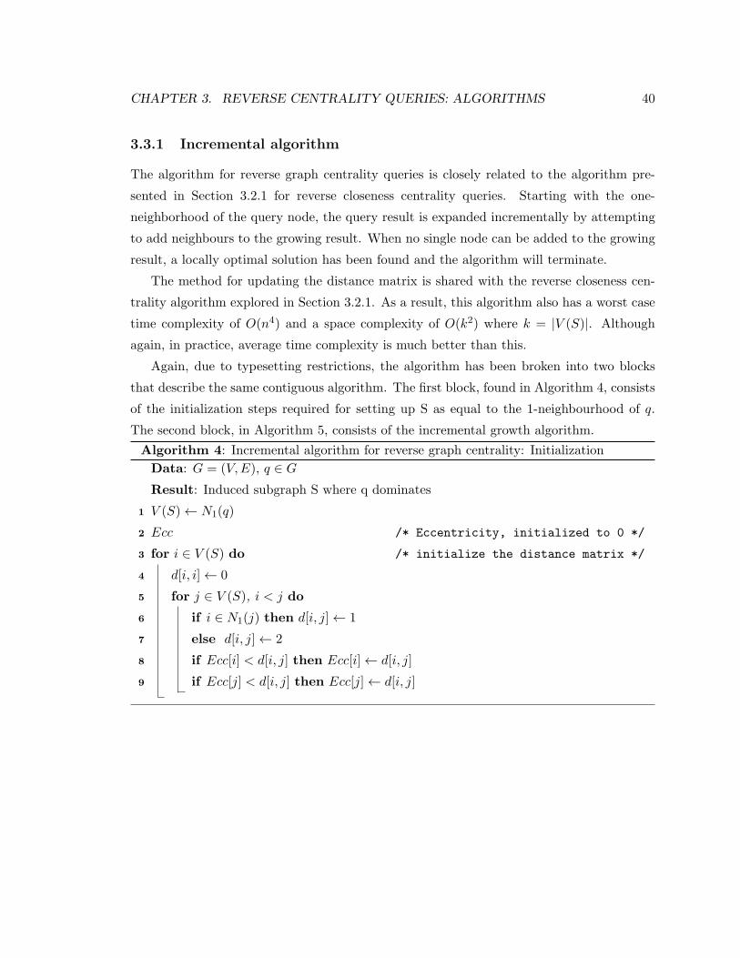
CHAPTER 3. REVERSE CENTRALITY QUERIES: ALGORITHMS 40
3.3.1 Incremental algorithm
The algorithm for reverse graph centrality queries is closely related to the algorithm pre-
sented in Section 3.2.1 for reverse closeness centrality queries. Starting with the one-
neighborhood of the query node, the query result is expanded incrementally by attempting
to add neighbours to the growing result. When no single node can be added to the growing
result, a locally optimal solution has been found and the algorithm will terminate.
The method for updating the distance matrix is shared with the reverse closeness cen-
trality algorithm explored in Section 3.2.1. As a result, this algorithm also has a worst case
time complexity of O(n4) and a space complexity of O(k2) where k = |V (S)|. Although
again, in practice, average time complexity is much better than this.
Again, due to typesetting restrictions, the algorithm has been broken into two blocks
that describe the same contiguous algorithm. The first block, found in Algorithm 4, consists
of the initialization steps required for setting up S as equal to the 1-neighbourhood of q.
The second block, in Algorithm 5, consists of the incremental growth algorithm.
Algorithm 4: Incremental algorithm for reverse graph centrality: Initialization
Data: G = (V,E), q ∈ G
Result: Induced subgraph S where q dominates
V (S)← N1(q)1
Ecc /* Eccentricity, initialized to 0 */2
for i ∈ V (S) do /* initialize the distance matrix */3
d[i, i]← 04
for j ∈ V (S), i < j do5
if i ∈ N1(j) then d[i, j]← 16
else d[i, j]← 27
if Ecc[i] < d[i, j] then Ecc[i]← d[i, j]8
if Ecc[j] < d[i, j] then Ecc[j]← d[i, j]9
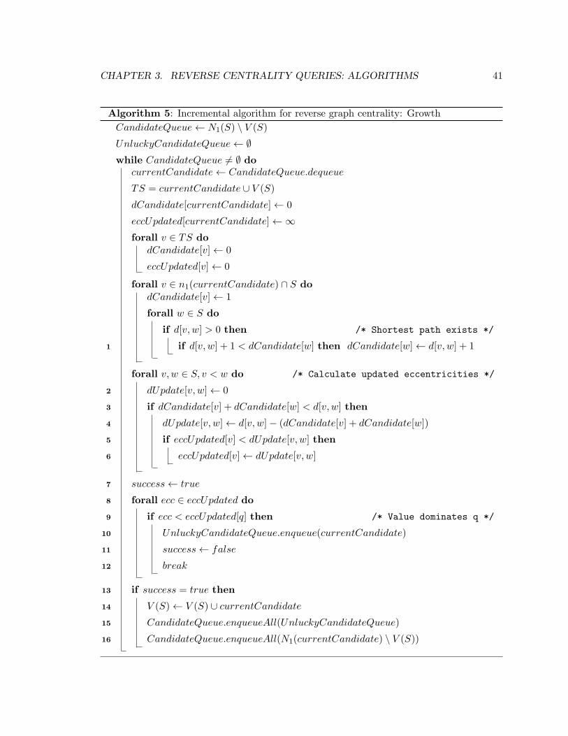
CHAPTER 3. REVERSE CENTRALITY QUERIES: ALGORITHMS 41
Algorithm 5: Incremental algorithm for reverse graph centrality: Growth
CandidateQueue← N1(S) \ V (S)
UnluckyCandidateQueue← ∅while CandidateQueue = ∅ do
currentCandidate← CandidateQueue.dequeue
TS = currentCandidate ∪ V (S)
dCandidate[currentCandidate]← 0
eccUpdated[currentCandidate]←∞forall v ∈ TS do
dCandidate[v]← 0
eccUpdated[v]← 0
forall v ∈ n1(currentCandidate) ∩ S dodCandidate[v]← 1
forall w ∈ S do
if d[v, w] > 0 then /* Shortest path exists */
if d[v, w] + 1 < dCandidate[w] then dCandidate[w]← d[v, w] + 11
forall v, w ∈ S, v < w do /* Calculate updated eccentricities */
dUpdate[v, w]← 02
if dCandidate[v] + dCandidate[w] < d[v, w] then3
dUpdate[v, w]← d[v, w]− (dCandidate[v] + dCandidate[w])4
if eccUpdated[v] < dUpdate[v, w] then5
eccUpdated[v]← dUpdate[v, w]6
success← true7
forall ecc ∈ eccUpdated do8
if ecc < eccUpdated[q] then /* Value dominates q */9
UnluckyCandidateQueue.enqueue(currentCandidate)10
success← false11
break12
if success = true then13
V (S)← V (S) ∪ currentCandidate14
CandidateQueue.enqueueAll(UnluckyCandidateQueue)15
CandidateQueue.enqueueAll(N1(currentCandidate) \ V (S))16
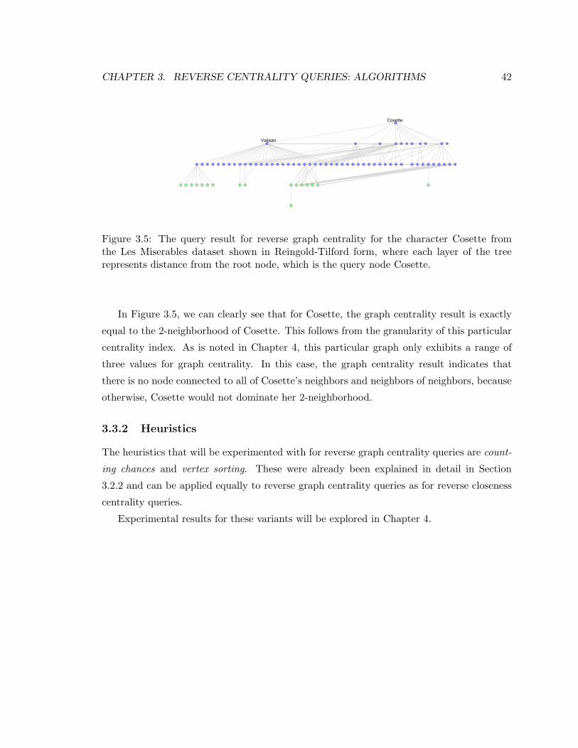
CHAPTER 3. REVERSE CENTRALITY QUERIES: ALGORITHMS 42
Figure 3.5: The query result for reverse graph centrality for the character Cosette fromthe Les Miserables dataset shown in Reingold-Tilford form, where each layer of the treerepresents distance from the root node, which is the query node Cosette.
In Figure 3.5, we can clearly see that for Cosette, the graph centrality result is exactly
equal to the 2-neighborhood of Cosette. This follows from the granularity of this particular
centrality index. As is noted in Chapter 4, this particular graph only exhibits a range of
three values for graph centrality. In this case, the graph centrality result indicates that
there is no node connected to all of Cosette’s neighbors and neighbors of neighbors, because
otherwise, Cosette would not dominate her 2-neighborhood.
3.3.2 Heuristics
The heuristics that will be experimented with for reverse graph centrality queries are count-
ing chances and vertex sorting. These were already been explained in detail in Section
3.2.2 and can be applied equally to reverse graph centrality queries as for reverse closeness
centrality queries.
Experimental results for these variants will be explored in Chapter 4.
Chapter 4
Experimental Results and
Discussion
4.1 Datasets
Zachary Karate Club dataset
The Zachary Karate Club dataset [52], introduced in Chapter 2, contains 34 nodes from a
karate club whose dynamics were studied in depth by W. W. Zachary. Links in this dataset
represent friendships or allegiances between members of the university karate club of an
unnamed American university. This network displays classical social network properties,
with a community clustering coefficient of 0.256, a power-law degree distribution as seen in
Figure 4.1a, and an average path length of 2.40. A visualization of this graph is provided
in Figure 2.1.
Les Miserables dataset
The Les Miserables dataset [32] includes 76 nodes representing characters in the eponymous
novel by Victor Hugo. Links in the dataset represent co-appearances in scenes in the novel.
This network displays classical social network properties, with a community clustering coef-
ficient of 0.499, a power-law degree distribution as seen in Figure 4.1b, and an average path
length of 2.64. A visualization of this graph is provided in Figure 1.1.
43
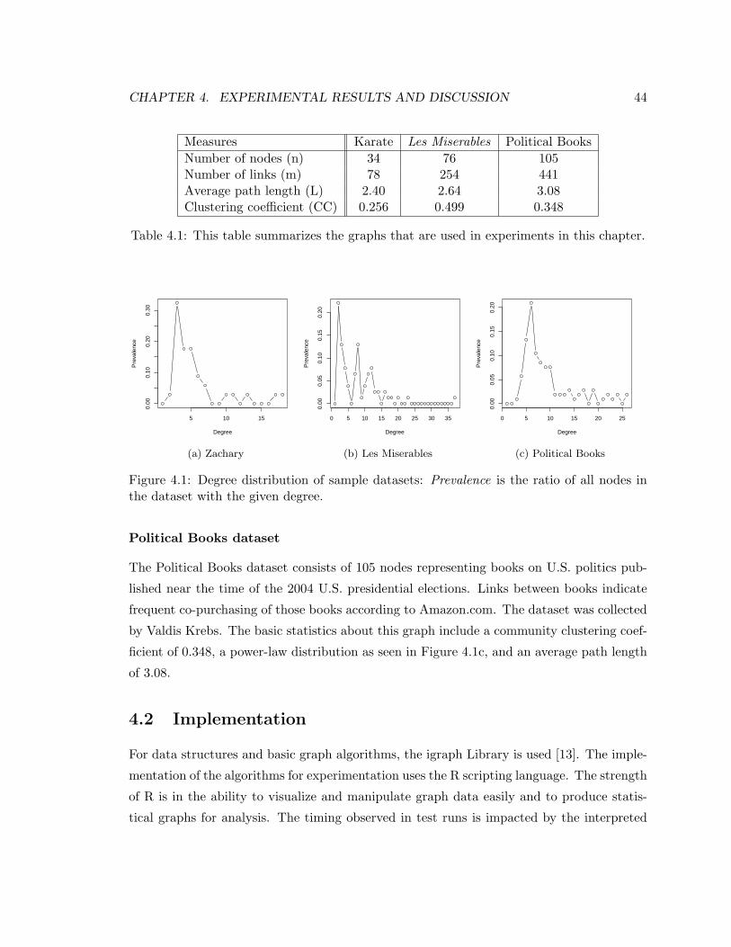
CHAPTER 4. EXPERIMENTAL RESULTS AND DISCUSSION 44
Measures Karate Les Miserables Political Books
Number of nodes (n) 34 76 105Number of links (m) 78 254 441Average path length (L) 2.40 2.64 3.08Clustering coefficient (CC) 0.256 0.499 0.348
Table 4.1: This table summarizes the graphs that are used in experiments in this chapter.
5 10 15
0.00
0.10
0.20
0.30
Degree
Pre
vale
nce
(a) Zachary
0 5 10 15 20 25 30 35
0.00
0.05
0.10
0.15
0.20
Degree
Pre
vale
nce
(b) Les Miserables
0 5 10 15 20 25
0.00
0.05
0.10
0.15
0.20
Degree
Pre
vale
nce
(c) Political Books
Figure 4.1: Degree distribution of sample datasets: Prevalence is the ratio of all nodes inthe dataset with the given degree.
Political Books dataset
The Political Books dataset consists of 105 nodes representing books on U.S. politics pub-
lished near the time of the 2004 U.S. presidential elections. Links between books indicate
frequent co-purchasing of those books according to Amazon.com. The dataset was collected
by Valdis Krebs. The basic statistics about this graph include a community clustering coef-
ficient of 0.348, a power-law distribution as seen in Figure 4.1c, and an average path length
of 3.08.
4.2 Implementation
For data structures and basic graph algorithms, the igraph Library is used [13]. The imple-
mentation of the algorithms for experimentation uses the R scripting language. The strength
of R is in the ability to visualize and manipulate graph data easily and to produce statis-
tical graphs for analysis. The timing observed in test runs is impacted by the interpreted
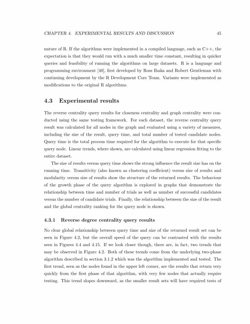
CHAPTER 4. EXPERIMENTAL RESULTS AND DISCUSSION 45
nature of R. If the algorithms were implemented in a compiled language, such as C++, the
expectation is that they would run with a much smaller time constant, resulting in quicker
queries and feasibility of running the algorithms on large datasets. R is a language and
programming environment [40], first developed by Ross Ihaka and Robert Gentleman with
continuing development by the R Development Core Team. Variants were implemented as
modifications to the original R algorithms.
4.3 Experimental results
The reverse centrality query results for closeness centrality and graph centrality were con-
ducted using the same testing framework. For each dataset, the reverse centrality query
result was calculated for all nodes in the graph and evaluated using a variety of measures,
including the size of the result, query time, and total number of tested candidate nodes.
Query time is the total process time required for the algorithm to execute for that specific
query node. Linear trends, where shown, are calculated using linear regression fitting to the
entire dataset.
The size of results versus query time shows the strong influence the result size has on the
running time. Transitivity (also known as clustering coefficient) versus size of results and
modularity versus size of results show the structure of the returned results. The behaviour
of the growth phase of the query algorithm is explored in graphs that demonstrate the
relationship between time and number of trials as well as number of successful candidates
versus the number of candidate trials. Finally, the relationship between the size of the result
and the global centrality ranking for the query node is shown.
4.3.1 Reverse degree centrality query results
No clear global relationship between query time and size of the returned result set can be
seen in Figure 4.2, but the overall speed of the query can be contrasted with the results
seen in Figures 4.4 and 4.15. If we look closer though, there are, in fact, two trends that
may be observed in Figure 4.2. Both of these trends come from the underlying two-phase
algorithm described in section 3.1.2 which was the algorithm implemented and tested. The
first trend, seen as the nodes found in the upper left corner, are the results that return very
quickly from the first phase of that algorithm, with very few nodes that actually require
testing. This trend slopes downward, as the smaller result sets will have required tests of
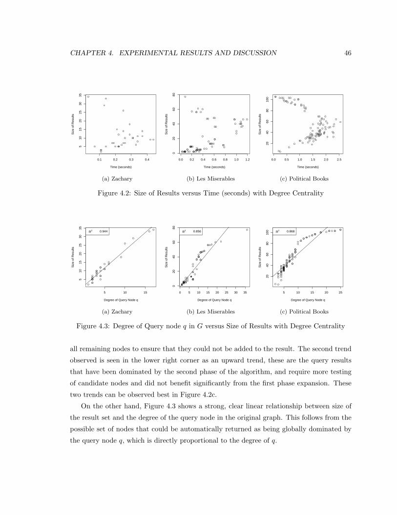
CHAPTER 4. EXPERIMENTAL RESULTS AND DISCUSSION 46
0.1 0.2 0.3 0.4
510
1520
2530
35
Time (seconds)
Siz
e of
Res
ults
(a) Zachary
0.0 0.2 0.4 0.6 0.8 1.0 1.2
020
4060
80
Time (seconds)S
ize
of R
esul
ts
(b) Les Miserables
0.0 0.5 1.0 1.5 2.0 2.5
2040
6080
100
Time (seconds)
Siz
e of
Res
ults
(c) Political Books
Figure 4.2: Size of Results versus Time (seconds) with Degree Centrality
5 10 15
510
1520
2530
35
Degree of Query Node q
Siz
e of
Res
ults
R2 0.944
(a) Zachary
0 5 10 15 20 25 30 35
020
4060
80
Degree of Query Node q
Siz
e of
Res
ults
R2 0.856
(b) Les Miserables
5 10 15 20 25
2040
6080
100
Degree of Query Node q
Siz
e of
Res
ults
R2 0.868
(c) Political Books
Figure 4.3: Degree of Query node q in G versus Size of Results with Degree Centrality
all remaining nodes to ensure that they could not be added to the result. The second trend
observed is seen in the lower right corner as an upward trend, these are the query results
that have been dominated by the second phase of the algorithm, and require more testing
of candidate nodes and did not benefit significantly from the first phase expansion. These
two trends can be observed best in Figure 4.2c.
On the other hand, Figure 4.3 shows a strong, clear linear relationship between size of
the result set and the degree of the query node in the original graph. This follows from the
possible set of nodes that could be automatically returned as being globally dominated by
the query node q, which is directly proportional to the degree of q.
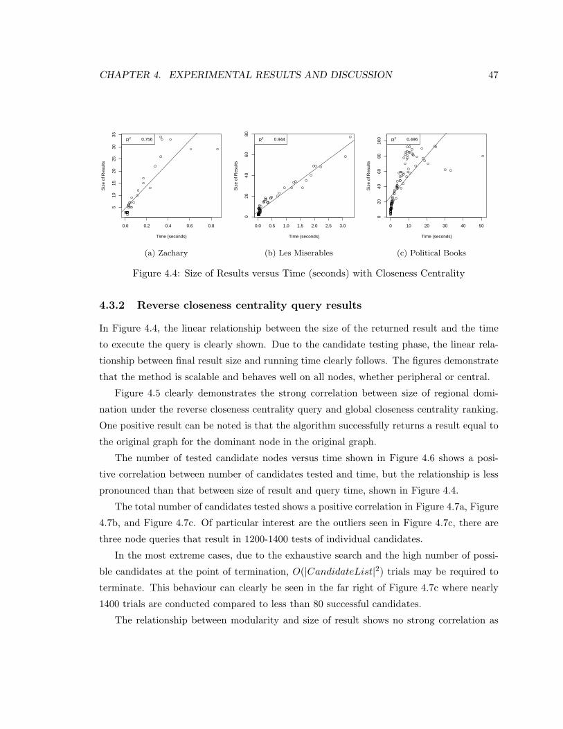
CHAPTER 4. EXPERIMENTAL RESULTS AND DISCUSSION 47
0.0 0.2 0.4 0.6 0.8
510
1520
2530
35
Time (seconds)
Siz
e of
Res
ults
R2 0.756
(a) Zachary
0.0 0.5 1.0 1.5 2.0 2.5 3.0
020
4060
80
Time (seconds)S
ize
of R
esul
ts
R2 0.944
(b) Les Miserables
0 10 20 30 40 50
020
4060
8010
0
Time (seconds)
Siz
e of
Res
ults
R2 0.496
(c) Political Books
Figure 4.4: Size of Results versus Time (seconds) with Closeness Centrality
4.3.2 Reverse closeness centrality query results
In Figure 4.4, the linear relationship between the size of the returned result and the time
to execute the query is clearly shown. Due to the candidate testing phase, the linear rela-
tionship between final result size and running time clearly follows. The figures demonstrate
that the method is scalable and behaves well on all nodes, whether peripheral or central.
Figure 4.5 clearly demonstrates the strong correlation between size of regional domi-
nation under the reverse closeness centrality query and global closeness centrality ranking.
One positive result can be noted is that the algorithm successfully returns a result equal to
the original graph for the dominant node in the original graph.
The number of tested candidate nodes versus time shown in Figure 4.6 shows a posi-
tive correlation between number of candidates tested and time, but the relationship is less
pronounced than that between size of result and query time, shown in Figure 4.4.
The total number of candidates tested shows a positive correlation in Figure 4.7a, Figure
4.7b, and Figure 4.7c. Of particular interest are the outliers seen in Figure 4.7c, there are
three node queries that result in 1200-1400 tests of individual candidates.
In the most extreme cases, due to the exhaustive search and the high number of possi-
ble candidates at the point of termination, O(|CandidateList|2) trials may be required to
terminate. This behaviour can clearly be seen in the far right of Figure 4.7c where nearly
1400 trials are conducted compared to less than 80 successful candidates.
The relationship between modularity and size of result shows no strong correlation as
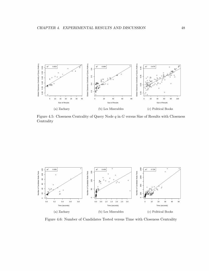
CHAPTER 4. EXPERIMENTAL RESULTS AND DISCUSSION 48
5 10 15 20 25 30 35
0.30
0.35
0.40
0.45
0.50
0.55
Size of Results
Glo
bal C
lose
ness
Cen
tral
ity o
f Que
ry N
ode
q
R2 0.833
(a) Zachary
0 20 40 60 80
0.3
0.4
0.5
0.6
Size of Results
Glo
bal C
lose
ness
Cen
tral
ity o
f Que
ry N
ode
q
R2 0.684
(b) Les Miserables
0 20 40 60 80 100
0.25
0.30
0.35
0.40
Size of Results
Glo
bal C
lose
ness
Cen
tral
ity o
f Que
ry N
ode
q
R2 0.679
(c) Political Books
Figure 4.5: Closeness Centrality of Query Node q in G versus Size of Results with ClosenessCentrality
0.0 0.2 0.4 0.6 0.8
020
4060
8010
012
0
Time (seconds)
Num
ber
of C
andi
date
Nod
e Te
sts
R2 0.595
(a) Zachary
0.0 0.5 1.0 1.5 2.0 2.5 3.0
050
100
150
Time (seconds)
Num
ber
of C
andi
date
Nod
e Te
sts
R2 0.436
(b) Les Miserables
0 10 20 30 40 50
020
060
010
0014
00
Time (seconds)
Num
ber
of C
andi
date
Nod
e Te
sts
R2 0.728
(c) Political Books
Figure 4.6: Number of Candidates Tested versus Time with Closeness Centrality
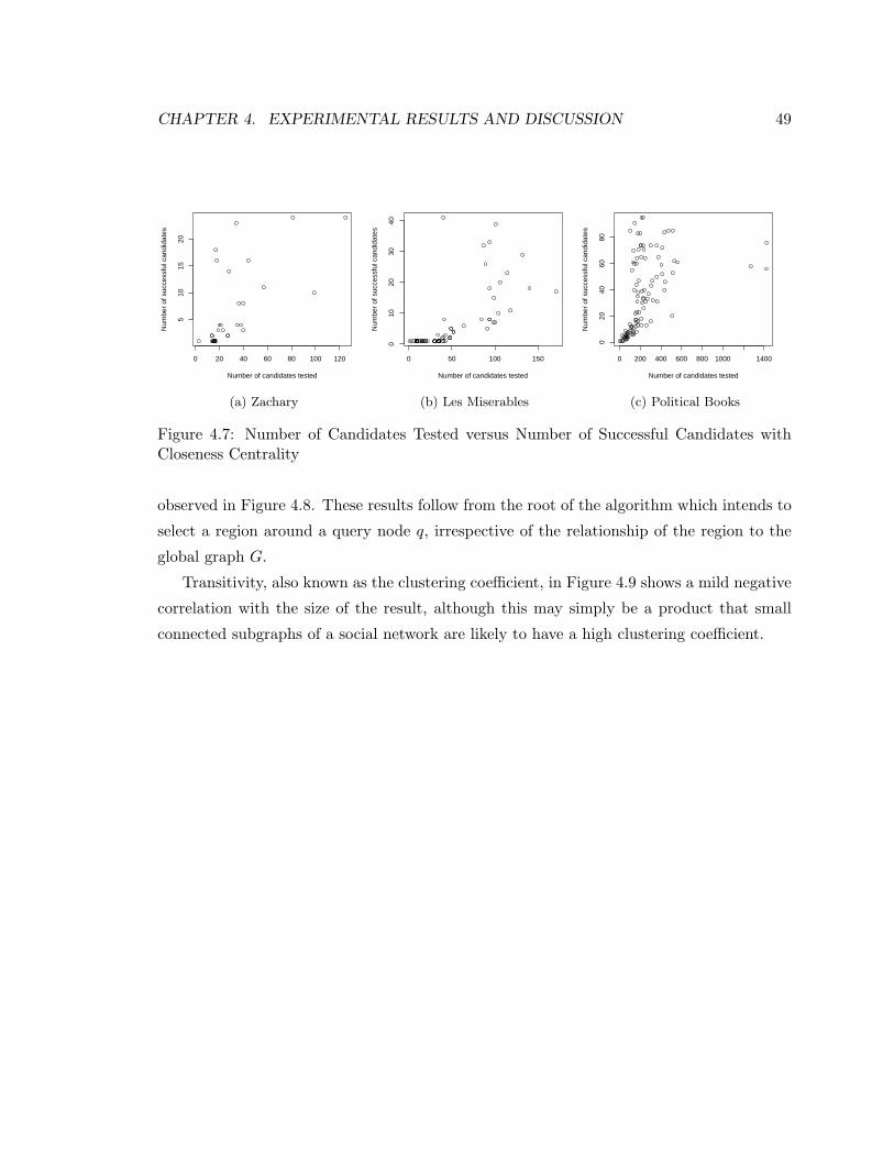
CHAPTER 4. EXPERIMENTAL RESULTS AND DISCUSSION 49
0 20 40 60 80 100 120
510
1520
Number of candidates tested
Num
ber
of s
ucce
ssfu
l can
dida
tes
(a) Zachary
0 50 100 150
010
2030
40
Number of candidates testedN
umbe
r of
suc
cess
ful c
andi
date
s
(b) Les Miserables
0 200 400 600 800 1000 1400
020
4060
80
Number of candidates tested
Num
ber
of s
ucce
ssfu
l can
dida
tes
(c) Political Books
Figure 4.7: Number of Candidates Tested versus Number of Successful Candidates withCloseness Centrality
observed in Figure 4.8. These results follow from the root of the algorithm which intends to
select a region around a query node q, irrespective of the relationship of the region to the
global graph G.
Transitivity, also known as the clustering coefficient, in Figure 4.9 shows a mild negative
correlation with the size of the result, although this may simply be a product that small
connected subgraphs of a social network are likely to have a high clustering coefficient.
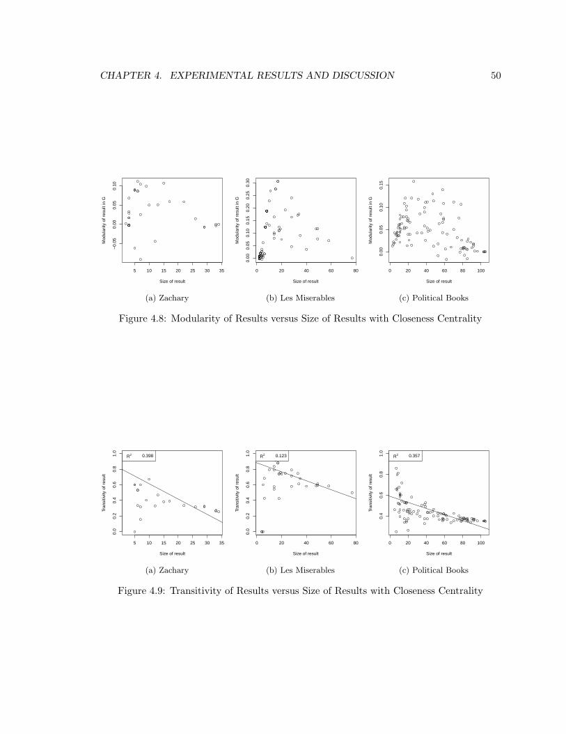
CHAPTER 4. EXPERIMENTAL RESULTS AND DISCUSSION 50
5 10 15 20 25 30 35
−0.
050.
000.
050.
10
Size of result
Mod
ular
ity o
f res
ult i
n G
(a) Zachary
0 20 40 60 80
0.00
0.05
0.10
0.15
0.20
0.25
0.30
Size of result
Mod
ular
ity o
f res
ult i
n G
(b) Les Miserables
0 20 40 60 80 100
0.00
0.05
0.10
0.15
Size of result
Mod
ular
ity o
f res
ult i
n G
(c) Political Books
Figure 4.8: Modularity of Results versus Size of Results with Closeness Centrality
5 10 15 20 25 30 35
0.0
0.2
0.4
0.6
0.8
1.0
Size of result
Tran
sitiv
ity o
f res
ult
R2 0.398
(a) Zachary
0 20 40 60 80
0.0
0.2
0.4
0.6
0.8
1.0
Size of result
Tran
sitiv
ity o
f res
ult
R2 0.123
(b) Les Miserables
0 20 40 60 80 100
0.4
0.6
0.8
1.0
Size of result
Tran
sitiv
ity o
f res
ult
R2 0.357
(c) Political Books
Figure 4.9: Transitivity of Results versus Size of Results with Closeness Centrality
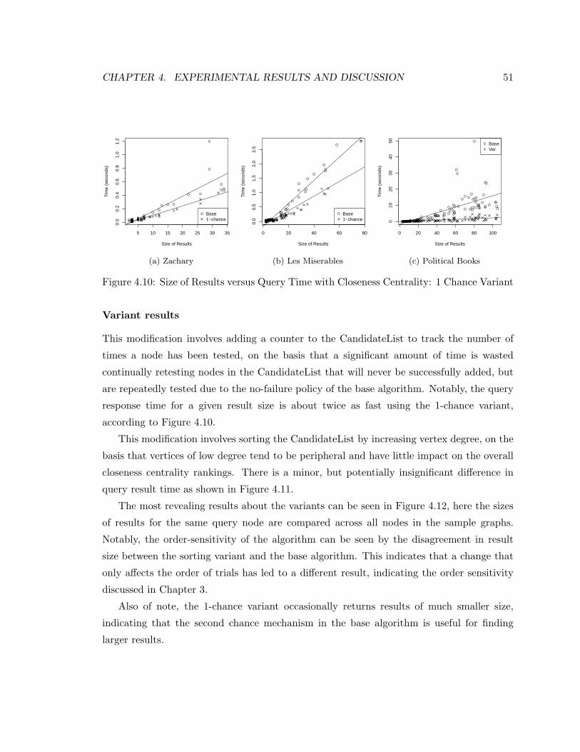
CHAPTER 4. EXPERIMENTAL RESULTS AND DISCUSSION 51
5 10 15 20 25 30 35
0.0
0.2
0.4
0.6
0.8
1.0
1.2
Size of Results
Tim
e (s
econ
ds)
Base1−chance
(a) Zachary
0 20 40 60 80
0.0
0.5
1.0
1.5
2.0
2.5
Size of ResultsT
ime
(sec
onds
)
Base1−chance
(b) Les Miserables
0 20 40 60 80 100
010
2030
4050
Size of Results
Tim
e (s
econ
ds)
BaseVar
(c) Political Books
Figure 4.10: Size of Results versus Query Time with Closeness Centrality: 1 Chance Variant
Variant results
This modification involves adding a counter to the CandidateList to track the number of
times a node has been tested, on the basis that a significant amount of time is wasted
continually retesting nodes in the CandidateList that will never be successfully added, but
are repeatedly tested due to the no-failure policy of the base algorithm. Notably, the query
response time for a given result size is about twice as fast using the 1-chance variant,
according to Figure 4.10.
This modification involves sorting the CandidateList by increasing vertex degree, on the
basis that vertices of low degree tend to be peripheral and have little impact on the overall
closeness centrality rankings. There is a minor, but potentially insignificant difference in
query result time as shown in Figure 4.11.
The most revealing results about the variants can be seen in Figure 4.12, here the sizes
of results for the same query node are compared across all nodes in the sample graphs.
Notably, the order-sensitivity of the algorithm can be seen by the disagreement in result
size between the sorting variant and the base algorithm. This indicates that a change that
only affects the order of trials has led to a different result, indicating the order sensitivity
discussed in Chapter 3.
Also of note, the 1-chance variant occasionally returns results of much smaller size,
indicating that the second chance mechanism in the base algorithm is useful for finding
larger results.
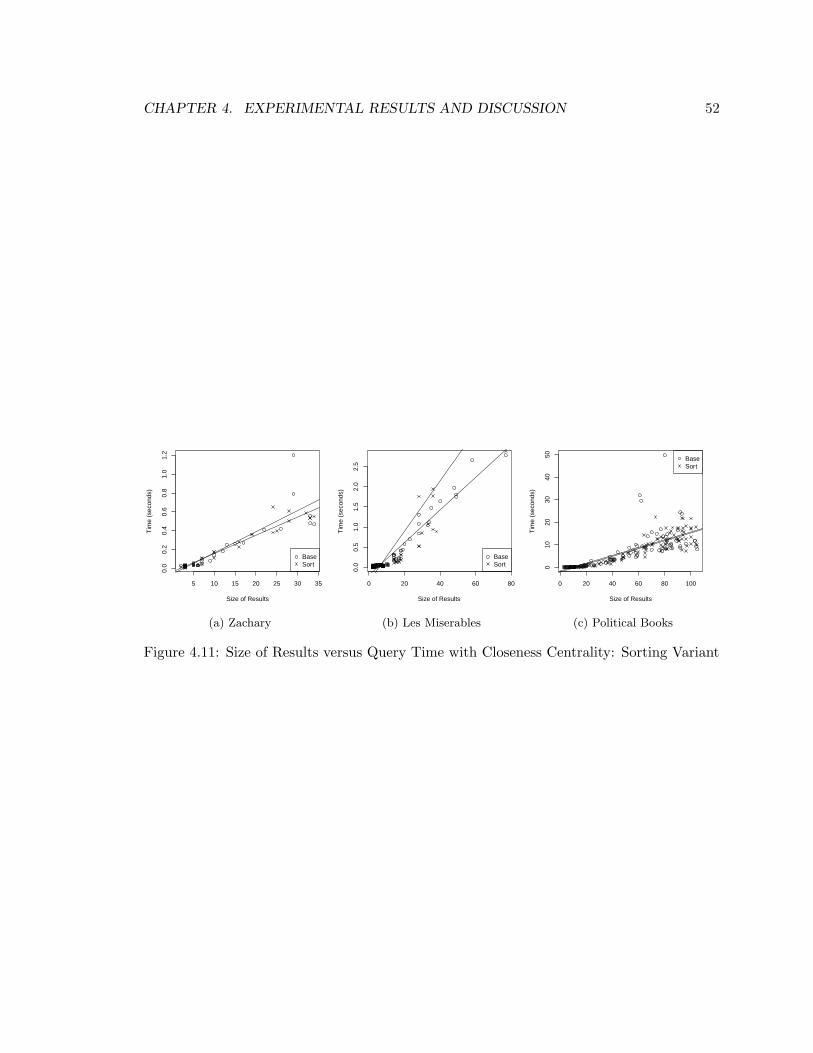
CHAPTER 4. EXPERIMENTAL RESULTS AND DISCUSSION 52
5 10 15 20 25 30 35
0.0
0.2
0.4
0.6
0.8
1.0
1.2
Size of Results
Tim
e (s
econ
ds)
BaseSort
(a) Zachary
0 20 40 60 80
0.0
0.5
1.0
1.5
2.0
2.5
Size of Results
Tim
e (s
econ
ds)
BaseSort
(b) Les Miserables
0 20 40 60 80 100
010
2030
4050
Size of Results
Tim
e (s
econ
ds)
BaseSort
(c) Political Books
Figure 4.11: Size of Results versus Query Time with Closeness Centrality: Sorting Variant
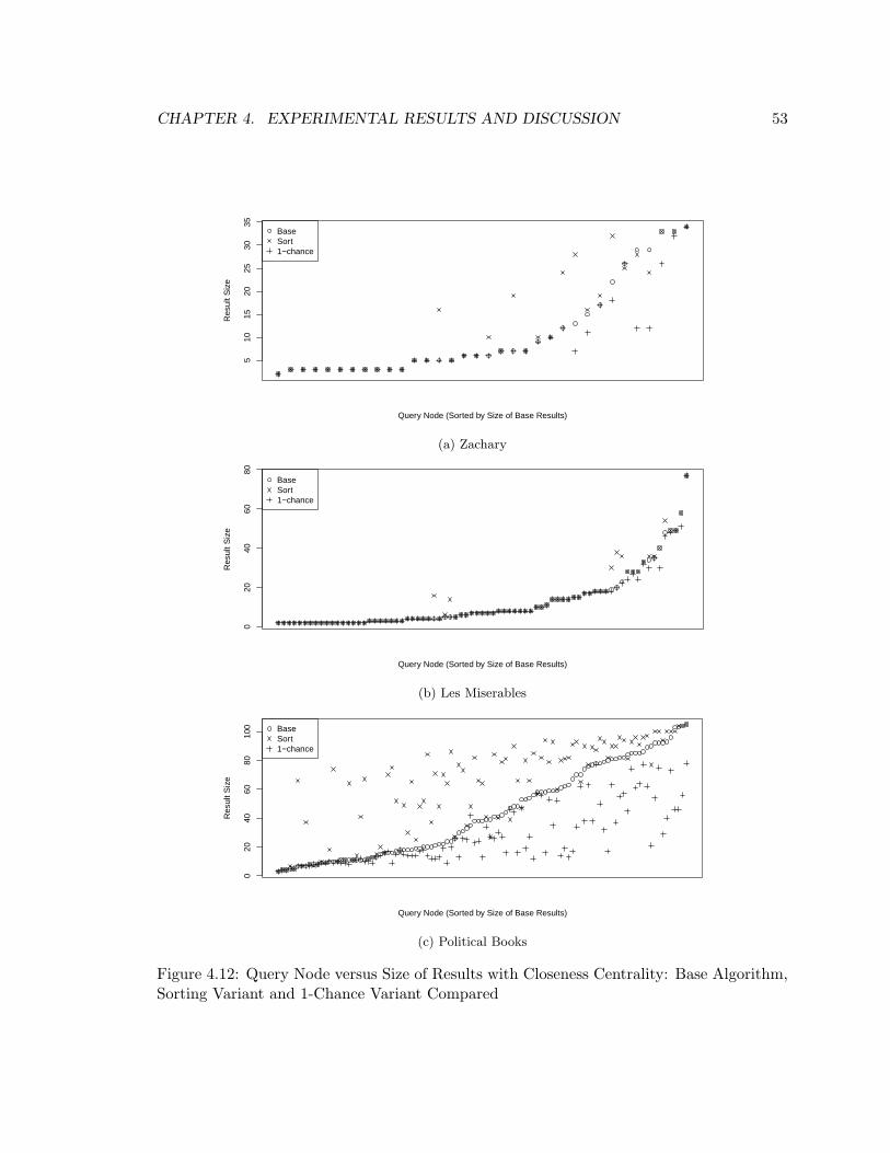
CHAPTER 4. EXPERIMENTAL RESULTS AND DISCUSSION 53
510
1520
2530
35
Query Node (Sorted by Size of Base Results)
Res
ult S
ize
BaseSort1−chance
(a) Zachary
020
4060
80
Query Node (Sorted by Size of Base Results)
Res
ult S
ize
BaseSort1−chance
(b) Les Miserables
020
4060
8010
0
Query Node (Sorted by Size of Base Results)
Res
ult S
ize
BaseSort1−chance
(c) Political Books
Figure 4.12: Query Node versus Size of Results with Closeness Centrality: Base Algorithm,Sorting Variant and 1-Chance Variant Compared
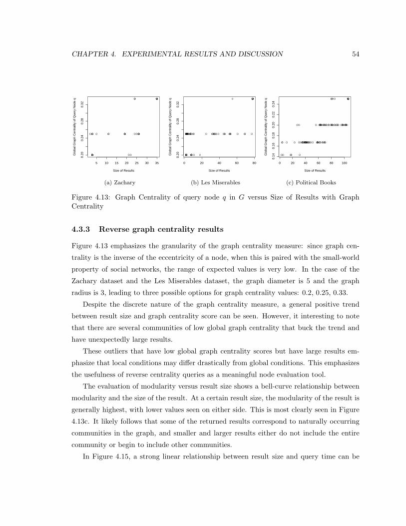
CHAPTER 4. EXPERIMENTAL RESULTS AND DISCUSSION 54
5 10 15 20 25 30 35
0.20
0.24
0.28
0.32
Size of Results
Glo
bal G
raph
Cen
tral
ity o
f Que
ry N
ode
q
(a) Zachary
0 20 40 60 80
0.20
0.24
0.28
0.32
Size of ResultsG
loba
l Gra
ph C
entr
ality
of Q
uery
Nod
e q
(b) Les Miserables
0 20 40 60 80 100
0.14
0.16
0.18
0.20
0.22
0.24
Size of Results
Glo
bal G
raph
Cen
tral
ity o
f Que
ry N
ode
q
(c) Political Books
Figure 4.13: Graph Centrality of query node q in G versus Size of Results with GraphCentrality
4.3.3 Reverse graph centrality results
Figure 4.13 emphasizes the granularity of the graph centrality measure: since graph cen-
trality is the inverse of the eccentricity of a node, when this is paired with the small-world
property of social networks, the range of expected values is very low. In the case of the
Zachary dataset and the Les Miserables dataset, the graph diameter is 5 and the graph
radius is 3, leading to three possible options for graph centrality values: 0.2, 0.25, 0.33.
Despite the discrete nature of the graph centrality measure, a general positive trend
between result size and graph centrality score can be seen. However, it interesting to note
that there are several communities of low global graph centrality that buck the trend and
have unexpectedly large results.
These outliers that have low global graph centrality scores but have large results em-
phasize that local conditions may differ drastically from global conditions. This emphasizes
the usefulness of reverse centrality queries as a meaningful node evaluation tool.
The evaluation of modularity versus result size shows a bell-curve relationship between
modularity and the size of the result. At a certain result size, the modularity of the result is
generally highest, with lower values seen on either side. This is most clearly seen in Figure
4.13c. It likely follows that some of the returned results correspond to naturally occurring
communities in the graph, and smaller and larger results either do not include the entire
community or begin to include other communities.
In Figure 4.15, a strong linear relationship between result size and query time can be
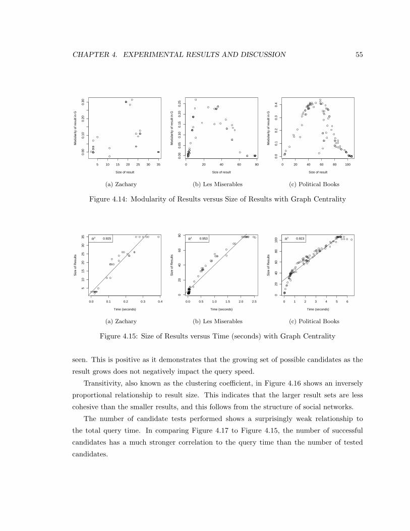
CHAPTER 4. EXPERIMENTAL RESULTS AND DISCUSSION 55
5 10 15 20 25 30 35
0.00
0.10
0.20
0.30
Size of result
Mod
ular
ity o
f res
ult i
n G
(a) Zachary
0 20 40 60 80
0.00
0.05
0.10
0.15
0.20
0.25
Size of resultM
odul
arity
of r
esul
t in
G
(b) Les Miserables
0 20 40 60 80 100
0.0
0.1
0.2
0.3
0.4
Size of result
Mod
ular
ity o
f res
ult i
n G
(c) Political Books
Figure 4.14: Modularity of Results versus Size of Results with Graph Centrality
0.0 0.1 0.2 0.3 0.4
510
1520
2530
35
Time (seconds)
Siz
e of
Res
ults
R2 0.925
(a) Zachary
0.0 0.5 1.0 1.5 2.0 2.5
020
4060
80
Time (seconds)
Siz
e of
Res
ults
R2 0.953
(b) Les Miserables
0 1 2 3 4 5 6
020
4060
8010
0
Time (seconds)
Siz
e of
Res
ults
R2 0.923
(c) Political Books
Figure 4.15: Size of Results versus Time (seconds) with Graph Centrality
seen. This is positive as it demonstrates that the growing set of possible candidates as the
result grows does not negatively impact the query speed.
Transitivity, also known as the clustering coefficient, in Figure 4.16 shows an inversely
proportional relationship to result size. This indicates that the larger result sets are less
cohesive than the smaller results, and this follows from the structure of social networks.
The number of candidate tests performed shows a surprisingly weak relationship to
the total query time. In comparing Figure 4.17 to Figure 4.15, the number of successful
candidates has a much stronger correlation to the query time than the number of tested
candidates.
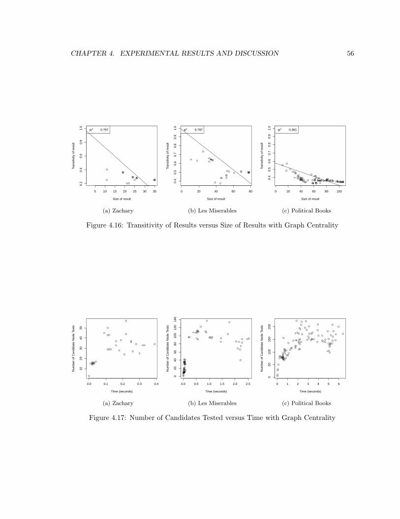
CHAPTER 4. EXPERIMENTAL RESULTS AND DISCUSSION 56
5 10 15 20 25 30 35
0.2
0.4
0.6
0.8
1.0
Size of result
Tran
sitiv
ity o
f res
ult
R2 0.797
(a) Zachary
0 20 40 60 80
0.4
0.5
0.6
0.7
0.8
0.9
1.0
Size of result
Tran
sitiv
ity o
f res
ult
R2 0.797
(b) Les Miserables
0 20 40 60 80 100
0.4
0.5
0.6
0.7
0.8
0.9
1.0
Size of result
Tran
sitiv
ity o
f res
ult
R2 0.361
(c) Political Books
Figure 4.16: Transitivity of Results versus Size of Results with Graph Centrality
0.0 0.1 0.2 0.3 0.4
1020
3040
50
Time (seconds)
Num
ber
of C
andi
date
Nod
e Te
sts
(a) Zachary
0.0 0.5 1.0 1.5 2.0 2.5
020
4060
8010
012
014
0
Time (seconds)
Num
ber
of C
andi
date
Nod
e Te
sts
(b) Les Miserables
0 1 2 3 4 5 6
050
100
150
200
Time (seconds)
Num
ber
of C
andi
date
Nod
e Te
sts
(c) Political Books
Figure 4.17: Number of Candidates Tested versus Time with Graph Centrality
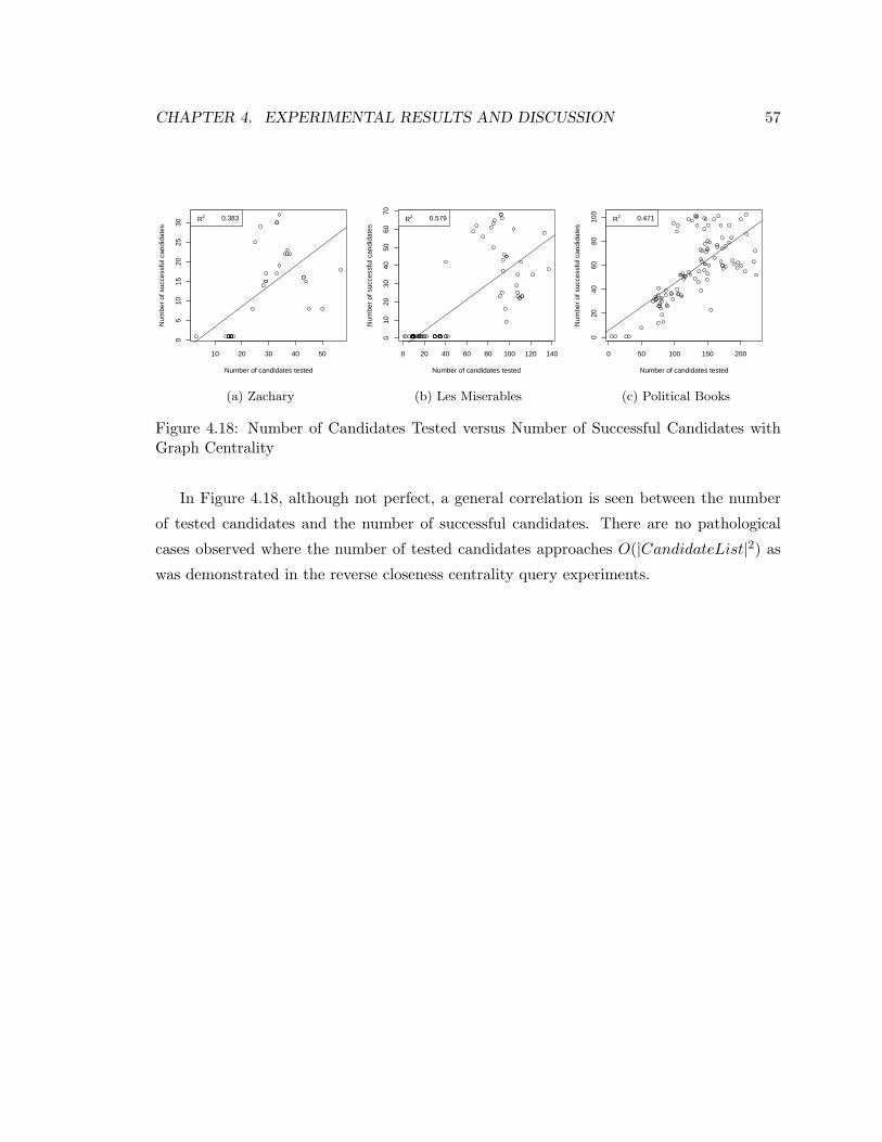
CHAPTER 4. EXPERIMENTAL RESULTS AND DISCUSSION 57
10 20 30 40 50
05
1015
2025
30
Number of candidates tested
Num
ber
of s
ucce
ssfu
l can
dida
tes
R2 0.383
(a) Zachary
0 20 40 60 80 100 120 140
010
2030
4050
6070
Number of candidates testedN
umbe
r of
suc
cess
ful c
andi
date
s
R2 0.579
(b) Les Miserables
0 50 100 150 200
020
4060
8010
0
Number of candidates tested
Num
ber
of s
ucce
ssfu
l can
dida
tes
R2 0.471
(c) Political Books
Figure 4.18: Number of Candidates Tested versus Number of Successful Candidates withGraph Centrality
In Figure 4.18, although not perfect, a general correlation is seen between the number
of tested candidates and the number of successful candidates. There are no pathological
cases observed where the number of tested candidates approaches O(|CandidateList|2) as
was demonstrated in the reverse closeness centrality query experiments.
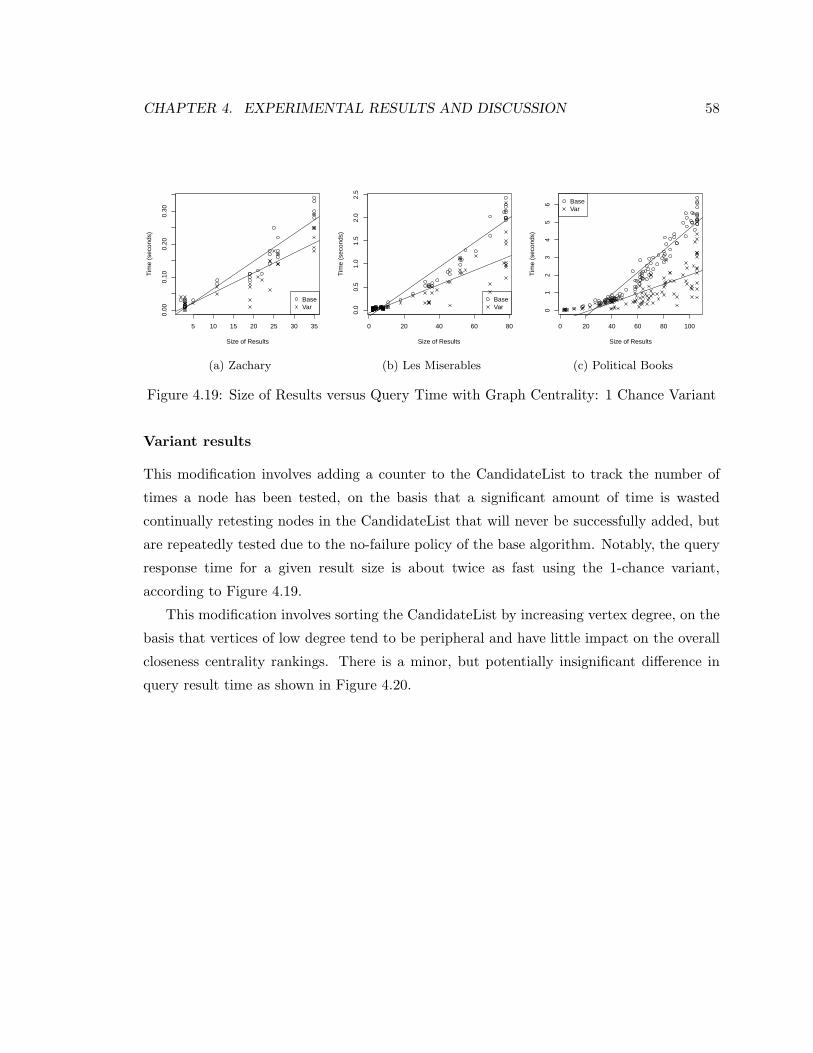
CHAPTER 4. EXPERIMENTAL RESULTS AND DISCUSSION 58
5 10 15 20 25 30 35
0.00
0.10
0.20
0.30
Size of Results
Tim
e (s
econ
ds)
BaseVar
(a) Zachary
0 20 40 60 80
0.0
0.5
1.0
1.5
2.0
2.5
Size of ResultsT
ime
(sec
onds
)
BaseVar
(b) Les Miserables
0 20 40 60 80 100
01
23
45
6
Size of Results
Tim
e (s
econ
ds)
BaseVar
(c) Political Books
Figure 4.19: Size of Results versus Query Time with Graph Centrality: 1 Chance Variant
Variant results
This modification involves adding a counter to the CandidateList to track the number of
times a node has been tested, on the basis that a significant amount of time is wasted
continually retesting nodes in the CandidateList that will never be successfully added, but
are repeatedly tested due to the no-failure policy of the base algorithm. Notably, the query
response time for a given result size is about twice as fast using the 1-chance variant,
according to Figure 4.19.
This modification involves sorting the CandidateList by increasing vertex degree, on the
basis that vertices of low degree tend to be peripheral and have little impact on the overall
closeness centrality rankings. There is a minor, but potentially insignificant difference in
query result time as shown in Figure 4.20.
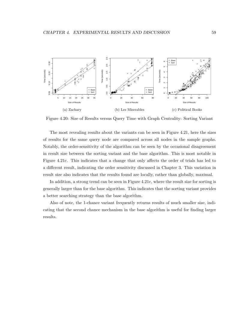
CHAPTER 4. EXPERIMENTAL RESULTS AND DISCUSSION 59
5 10 15 20 25 30 35
0.00
0.10
0.20
0.30
Size of Results
Tim
e (s
econ
ds)
BaseSort
(a) Zachary
0 20 40 60 80
0.0
0.5
1.0
1.5
2.0
2.5
Size of ResultsT
ime
(sec
onds
)
BaseSort
(b) Les Miserables
0 20 40 60 80 100
01
23
45
6
Size of Results
Tim
e (s
econ
ds)
BaseSort
(c) Political Books
Figure 4.20: Size of Results versus Query Time with Graph Centrality: Sorting Variant
The most revealing results about the variants can be seen in Figure 4.21, here the sizes
of results for the same query node are compared across all nodes in the sample graphs.
Notably, the order-sensitivity of the algorithm can be seen by the occasional disagreement
in result size between the sorting variant and the base algorithm. This is most notable in
Figure 4.21c. This indicates that a change that only affects the order of trials has led to
a different result, indicating the order sensitivity discussed in Chapter 3. This variation in
result size also indicates that the results found are locally, rather than globally, maximal.
In addition, a strong trend can be seen in Figure 4.21c, where the result size for sorting is
generally larger than for the base algorithm. This indicates that the sorting variant provides
a better searching strategy than the base algorithm.
Also of note, the 1-chance variant frequently returns results of much smaller size, indi-
cating that the second chance mechanism in the base algorithm is useful for finding larger
results.
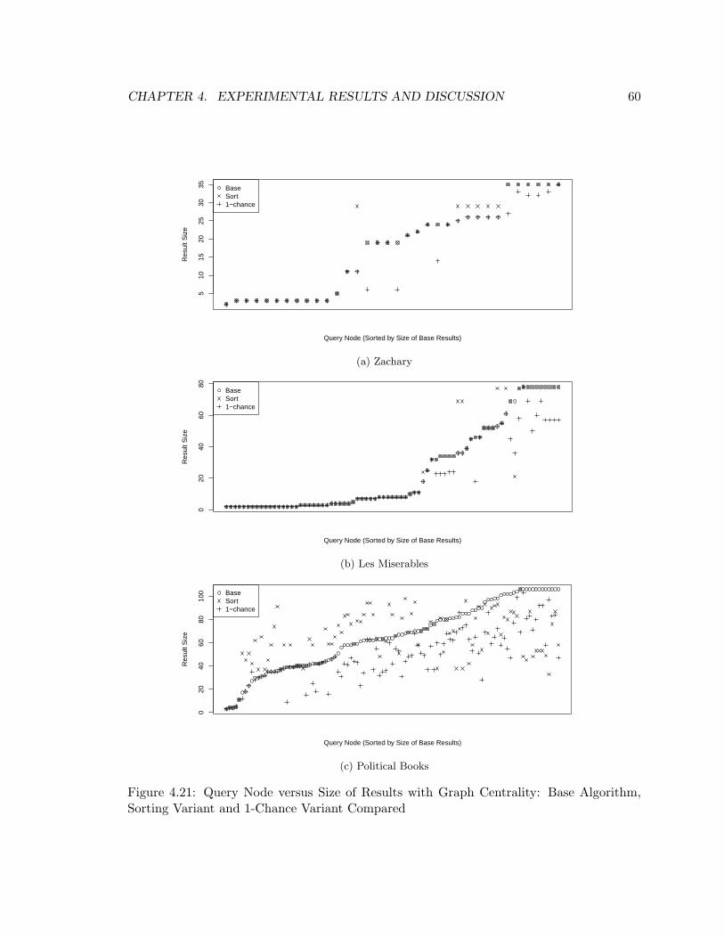
CHAPTER 4. EXPERIMENTAL RESULTS AND DISCUSSION 60
510
1520
2530
35
Query Node (Sorted by Size of Base Results)
Res
ult S
ize
BaseSort1−chance
(a) Zachary
020
4060
80
Query Node (Sorted by Size of Base Results)
Res
ult S
ize
BaseSort1−chance
(b) Les Miserables
020
4060
8010
0
Query Node (Sorted by Size of Base Results)
Res
ult S
ize
BaseSort1−chance
(c) Political Books
Figure 4.21: Query Node versus Size of Results with Graph Centrality: Base Algorithm,Sorting Variant and 1-Chance Variant Compared
CHAPTER 4. EXPERIMENTAL RESULTS AND DISCUSSION 61
4.3.4 Reverse centrality queries versus global centrality
Reverse centrality queries provide novel information at the node level, which may signif-
icantly differ from the information available with respect to the entire graph. There are
cases where a globally insignificant node may play an important part in its own local region.
With that, the context of the query node is given greater importance due to local centrality,
whereas the same node may seem relatively insignificant at the global level.
4.4 Summary
This chapter began by introducing the three datasets that were used for experimental anal-
ysis. The implementation in R used for experimentation was described in Section 4.2.
Finally, detailed experimental analysis was provided on the three query types across the
three datasets introduced in the beginning of the chapter.
In summary, the major insights we gained from our experimental results are:
• In Section 4.3.1, we established the reverse degree centrality query method provides
query results very quickly for all datasets explored. Additionally, we verified the
expected linear relationship between result size and query node degree.
• Exploring reverse closeness centrality queries in Section 4.3.2, we saw a general lin-
ear relationship between result size and query time, but several pathological cases
were noted in the Political Books dataset. The presence of outliers in Figure 4.5
demonstrates that there are cases where nodes of low global closeness centrality can
dominate large regions. The counting chances variant was demonstrated to be an
effective method for significantly reducing query time, but at the expense of occasion-
ally smaller result sizes. The sorting variant was shown to perhaps marginally improve
query times, but more importantly, also occasionally produced larger results than the
base method.
• In Section 4.3.3, for reverse graph centrality queries, we established a strong linear
relationship between result size and query running time. The counting chances variant
proved to be useful in reducing query time, but also occasionally reduced the result
size. The sorting variant performed slightly worse than the base method, indicating
that sorting by vertex degree is not an appropriate heuristic for graph centrality.

CHAPTER 4. EXPERIMENTAL RESULTS AND DISCUSSION 62
Outliers in Figure 4.13 demonstrate that nodes of low graph centrality, usually nodes
considered peripheral to the graph, occasionally return large results, demonstrating
strong local dominance under graph centrality.
Chapter 5
Conclusion and Future Work
5.1 Summary
The rapid growth in the volume and availability of complex network data provides us with
many opportunities to define new paradigms for exploring and understanding this data. Re-
verse centrality queries provide another analysis tool for understanding the complex struc-
ture and dynamics of a social network, especially in relation to individual nodes in the
network. The methods presented in this thesis provide new methods for answering these
novel queries.
We conclude by briefly summarizing the major contributions of this thesis:
• In Chapter 2, we introduced a novel query type for social network analysis called the
reverse centrality query.
• In Chapter 3, we gave incremental algorithms for finding locally optimal query results
for three types of reverse centrality queries.
• In Chapter 4, we provided a detailed analysis of the results of the three query types
on three real-world networks and demonstrated the queries provide an effective novel
means of graph exploration.
• In Section 5.2, we provide a wide number of future directions in which reverse centrality
queries may be improved in the future.
63

CHAPTER 5. CONCLUSION AND FUTURE WORK 64
5.2 Future work
In this thesis, we introduced reverse centrality queries, and provided a detailed treatment
of several aspects of these queries. There are many potential directions for future work in
this area. Further heuristic improvements to the methods presented in Chapter 3 may be
possible. Additional modifications to adapt the given methods to run efficiently on large
graphs would also be useful. In Chapter 2, we outlined several types of constraints that could
be added to the problem definition of reverse centrality queries. A detailed treatment of these
constraints, including experimentation and evaluation would be beneficial. The methods
of Chapter 3 use a basic breadth first search approach, a more sophisticated approach
that incorporates back-tracking is likely to improve the query result by searching more of
the problem space. These methods do provide a way to answer several types of reverse
centrality queries, but they are limited in their applicability due to time complexity issues.
An important future direction is the development of more efficient methods to increase the
size of graph that can be queried.
5.2.1 Heuristic improvements
For all algorithms, improvements may be found by using statistics which are pre-computed
on the whole graph, or on the connected component of the graph that the query node is
found in.
Global statistics
Using global centrality indices such as betweenness centrality, or other statistics such as
vertex degree and local density may help improve the efficiency of the algorithm in finding
large regions. Other static statistics may also heuristically improve our methods. These
statistics would be used to sort the candidate list, changing the search priority of the method.
Positive indicators such as low vertex degree may be used to indicate peripheral nodes
in the graph that can very likely be added without disrupting the dominance of the query
node. The sorting variant seen in Chapters 3 and 4 for graph and closeness centralities is
based on the use of low vertex degree as a positive indicator.
Negative indicators, such as high betweenness centrality may be used to identify influen-
tial nodes which are likely to dominate the query node. If a node dominates the query node
CHAPTER 5. CONCLUSION AND FUTURE WORK 65
in the global graph, it is very likely that that node will not contribute to the dominance
region of the query node except possibly as a peripheral node.
Partitioning
Another option is to pre-process the graph into community partitions and only consider
nodes within the query point’s own partition. This could additionally reduce query time by
reducing the size of the set of candidate nodes. In addition, partitioning would be a useful
means for reducing the query time on larger datasets. Partitioning could also improve the
performance of static statistics used heuristically in node selection in the two methods.
5.2.2 Feature vector networks
An extension that is possible for the future is the adaptation of these methods for feature
vector networks, where each node in the network has an associated feature vector. This
would allow more powerful queries to be run on the social network which are additionally
constrained by vector attributes.
5.2.3 Advanced search methods
The algorithms presented in Chapter 3 use a straight forward breadth first search technique
to identify nodes to add to the result set, improved by revisiting all potential candidate
nodes. This method could be further modified to allow back-tracking: the removal of
successful candidates to explore other search paths.
5.2.4 Variants on reverse centrality query answering
By limiting the expansion of the search to a fixed radius k, we can decrease the number of
possible iterations required to find an answer. This is especially useful in large graphs where
an answer may potentially be the entire graph and calculating this could be prohibitively
expensive.
These same methods can be used to generate multiple answers by varying k from 2 to
r, a user defined maximum radius. This parameter will be very small in practice due to the
(small world) nature of most complex networks.
Another way to improve query answering time would be to restrict the size of the re-
sulting answer to a fixed number of nodes, where |V (S)| < h, and h is a constant. This
CHAPTER 5. CONCLUSION AND FUTURE WORK 66
technique may be useful in preliminary evaluation to see whether the node dominates a
large area or not.
5.2.5 Local Centrality Measures
An idea briefly introduced in Definition 2.6.5 is that of local centrality. No available measure
that I am aware of properly quantifies this idea. I believe that this is a very fruitful future
research direction. The experimental results of this thesis demonstrate that there are indeed
nodes that are capable of dominating large regions, while showing only modest centrality in
the global graph.
Appendix A
Appendix 1
A.1 The All-Pairs Shortest Path (APSP) Problem
The all-pairs shortest path (APSP) problem involves finding the shortest paths between
all pairs of nodes in a graph. The APSP problem is directly related to distance-based and
path-based centrality indices. Determining the exact radius of the graph requires knowledge
of the longest shortest path (the eccentricity) for each node in the graph. Since the graph
centrality problem requires knowing the nodes that have eccentricity equal to the radius
of the graph, it follows that we must know the eccentricity of every node in the graph. It
follows that the graph center can be trivially calculated from knowing APSP for a given
graph. So the problem of determining the graph centrality in the general graph is bounded
by the complexity of the APSP problem.
Purpose-built algorithms for finding graph centers have improved on the APSP com-
plexity bound for specific subclasses of graphs, including chordal [12], 3-cactus [30], and
HDD-free [11] graphs. These specific algorithms exploit special properties of these classes of
graphs to determine at least one central vertex, however, they do not return the full graph
center. Additionally, the constraints imposed by these graph classes are too strong to be
applied on any real world network.
The APSP problem is well-studied in the field of graph theory. The classic solution
of utilizing breadth-first search from every node is O(mn) or O(n3) since the number of
links, m, is bounded by m ≤ n(n − 1). Speed-ups for this method either use fast matrix
multiplication, such as Seidel’s algorithm [44] that runs in O(n2.376), or methods that give
logarithmic improvements over the classic method, such as Feder and Motwani’s O(n3/ log n)
67
APPENDIX A. APPENDIX 1 68
method [16] for unweighted, undirected graphs. The static version of APSP is relevant to
the reverse centrality query introduced in this thesis.
The recent work by Chan [10] has improved the complexity bound on the problem for
static sparse graphs with m ≪ n1.376. In particular, for graphs where m ≤ n log log n,
the method achieves O(n2 log2 log n/ log n), which is impressive given the naıve method is
O(n3).
Additional work by Boitmanis et al. [5] has established an additive approximation
algorithm with time bound O(km) with an additive error at most 2(n−1)k+1 , which leads to
an O(√nm) algorithm with at most O(
√n) additive error. Approximation algorithms use
multiple breadth-first searches from k nodes within the graph.
Dijkstra’s algorithm [15] can be used to solve the single-source shortest paths problem
in time O(m+ n log n) when implemented with Fibonacci heaps.
A.1.1 Changing Distances: Dynamic All-pairs Shortest Path
Most relevant to the graph center problem is the dynamic APSP problem, where vertices are
either being added or deleted. An update operation deals with one vertex and any incident
edges, an incremental operation only involves adding edges and a decremental operation
only involves deleting edges. The fully dynamic case of APSP is the most challenging, but
is beyond the scope of what is required for the reverse centrality query problem.
The fully dynamic APSP problem was addressed in a ground-breaking paper by Deme-
trescu and Italiano [14] that presents a fully dynamic algorithm based on maintaining locally
shortest and historical paths as the graph evolves and achieve updates in O(n2 log3 n).
An exploration of the methods for the incremental and decremental dynamic The APSP
problem is relevant to the problem of solving reverse centrality queries. Since we are required
to repeatedly re-calculate the vertices with highest centrality as the induced subgraph either
grows or shrinks under the searching method. The partially dynamic APSP problem is
luckily an easier problem to tackle than the fully-dynamic case.
For the decremental case, Thorup [46] introduces a basic algorithm that handles up to
j deletions in O(j3 log j) total time. The amortized cost per update for Thorup’s method
is thus O(j2 log j) over j deletions. The decremental algorithm is simplified by the guaran-
tee that any deleted vertex will only increase shortest paths between other vertices whose
shortest paths include the deleted vertex along the path.

APPENDIX A. APPENDIX 1 69
A simple algorithm for addition updates can be implemented by using Dijkstra’s algo-
rithm to calculate the single-source shortest path from the added node to all existing nodes
in O(m+ n log n) time and then updating the shortest-path distance matrix in O(n2) time.
This gives an update cost of O(n2) for additive updates.

Bibliography
[1] Colin Aldridge. The kawachi algorithm: A single-parameter network constructor? InThe 19th Annual Colloquium of the Spatial Information Research Centre (SIRC07),2007.
[2] Lars Backstrom, Dan Huttenlocher, Jon Kleinberg, and Xiangyang Lan. Group for-mation in large social networks: membership, growth, and evolution. In KDD ’06:Proceedings of the 12th ACM SIGKDD international conference on Knowledge discov-ery and data mining, pages 44–54, New York, NY, USA, 2006. ACM.
[3] Albert-Lszl Barabsi and Rka Albert. Emergence of scaling in random networks. Science,1999.
[4] Vladimir Batagelj. Pajek - analysis and visualization of large networks. Graph DrawingSoftware, pages 77–103, 2003. Jnger, M., Mutzel, P., (Eds.).
[5] Krists Boitmanis, Karlis Freivalds, Peteris Ledins, and Rudolfs Opmanis. Fast and sim-ple approximation of the diameter and radius of a graph. In Workshop on Experimentaland Efficient Algorithms (WEA), pages 98–108, 2006.
[6] Phillip Bonacich. Power and centrality: A family of measures. The American Journalof Sociology, 92(5):1170–1182, March 1987.
[7] Ulrik Brandes. A faster algorithm for betweenness centrality. Journal of MathematicalSociology, 25:163–177, 2001.
[8] Ulrik Brandes and Thomas Erlebach. Network Analysis: Methodological Foundations.Springer, March 2005.
[9] Sergey Brin and Lawrence Page. The anatomy of a large-scale hypertextual web searchengine. Comput. Netw. ISDN Syst., 30(1-7):107–117, 1998.
[10] Timothy M. Chan. All-pairs shortest paths for unweighted undirected graphs in o(mn)time. In SODA ’06: Proceedings of the seventeenth annual ACM-SIAM symposium onDiscrete algorithm, pages 514–523, New York, NY, USA, 2006. ACM.
[11] Victor Chepoi and Feodor Dragan. Finding a central vertex in an hhd-free graph.Discrete Appl. Math., 131(1):93–111, 2003.
70
BIBLIOGRAPHY 71
[12] Victor Chepoi and Feodor F. Dragan. A linear-time algorithm for finding a centralvertex of a chordal graph. In ESA ’94: Proceedings of the Second Annual EuropeanSymposium on Algorithms, pages 159–170, London, UK, 1994. Springer-Verlag.
[13] Gabor Csardi and Tamas Nepusz. The igraph software package for complex networkresearch. InterJournal, Complex Systems:1695, 2006.
[14] Camil Demetrescu and Giuseppe F. Italiano. A new approach to dynamic all pairsshortest paths. J. ACM, 51(6):968–992, 2004.
[15] Edsger W. Dijkstra. A note on two problems in connexion with graphs. NumerischeMathematik, 1:269–271, 1959.
[16] Tomas Feder and Rajeev Motwani. Clique partitions, graph compression and speeding-up algorithms. In STOC ’91: Proceedings of the twenty-third annual ACM symposiumon Theory of computing, pages 123–133, New York, NY, USA, 1991. ACM.
[17] Gary William Flake, Steve Lawrence, and C. Lee Giles. Efficient identification of webcommunities. In Knowledge Discovery and Data Mining (KDD), pages 150–160, 2000.
[18] Gary William Flake, Steve Lawrence, C. Lee Giles, and Frans M. Coetzee. Self-organization and identification of web communities. IEEE Computer, 35:66–71, 2002.
[19] Linton C. Freeman. A set of measures of centrality based upon betweenness. Sociometry,40:35–41, 1977.
[20] Zhonghua Gao, Zhenjie Chen, Yongxue Liu, and Kang Huang. Study on the com-plex network characteristics of urban road system based on gis. Geoinformatics 2007:Geospatial Information Technology and Applications, 6754, 2007.
[21] David Gibson, Ravi Kumar, and Andrew Tomkins. Discovering large dense subgraphsin massive graphs. In VLDB ’05: Proceedings of the 31st international conference onVery large data bases, pages 721–732. VLDB Endowment, 2005.
[22] Michelle Girvan and Mark E. J. Newman. Community structure in social and biologicalnetworks. Proceedings of the National Academy of Sciences of the United States ofAmerica, 99(12):7821–7826, June 2002.
[23] Per Hage and Frank Harary. Eccentricity and centrality in networks. Social Networks,17(1):57–63, 1995.
[24] Jiawei Han and Micheline Kamber. Data Mining: Concepts and Techniques. MorganKaufmann, 2001.
[25] Woochang Hwang, Taehyong Kim, Murali Ramanathan, and Aidong Zhang. Bridgingcentrality: graph mining from element level to group level. In Knowledge Discoveryand Data Mining (KDD), pages 336–344, 2008.
BIBLIOGRAPHY 72
[26] David Jensen and Jennifer Neville. Data mining in social networks. In Papers of theSymposium on Dynamic Social Network Modeling and Analysis, Washington, DC, 2002.National Academy of Sciences, National Academy Press.
[27] Donald B. Johnson. Efficient algorithms for shortest paths in sparse networks. J. ACM,24(1):1–13, 1977.
[28] Yuumi Kawachi, Kenta Murara, Shinichiro Yoshi, and Yukinori Kakazu. The structuralphase transition among fixed cardinal networks. In In Proceedings of the 7th Asia-Pacific Conference on Complex Systems, page 247255, 2004.
[29] David Kempe, Jon Kleinberg, and Eva Tardos. Maximizing the spread of influencethrough a social network. In Knowledge Discovery and Data Mining (KDD), pages137–146, New York, NY, USA, 2003. ACM.
[30] Rex K. Kincaid and Oded Z. Maimon. A note on locating a central vertex of a 3-cactusgraph. Comput. Oper. Res., 17(3):315–320, 1990.
[31] Jon M. Kleinberg. Authoritative sources in a hyperlinked environment. J. ACM,46(5):604–632, 1999.
[32] D. E. Knuth. The Stanford GraphBase: A Platform for Combinatorial Computing.Addison-Wesley, Reading, MA, 1994.
[33] David Krackhardt. Assessing the political landscape: Structure, cognition, and powerin organizations. Administrative Science Quarterly, 35:342–369, 1990.
[34] Vito Latora and Massimo Marchiori. Efficient behavior of small-world networks. Phys.Rev. Lett., 87(19):198701, Oct 2001.
[35] Chong Liu, Kui Wu, and Jian Pei. An energy-efficient data collection framework forwireless sensor networks by exploiting spatiotemporal correlation. IEEE Transactionson Parallel and Distributed Systems, 18(7):1010–1023, 2007.
[36] Nina Mishra, Robert Schreiber, Isabelle Stanton, and Robert Endre Tarjan. Clusteringsocial networks. In WAW, pages 56–67, 2007.
[37] Flavia Moser, Rong Ge, and Martin Ester. Joint cluster analysis of attribute andrelationship data withouta-priori specification of the number of clusters. In KnowledgeDiscovery and Data Mining (KDD), pages 510–519, 2007.
[38] Mark E. J. Newman. The structure and function of complex networks. SIAM Review,45(167), 2003.
[39] Mark E. J. Newman. Fast algorithm for detecting community structure in networks.Physical Review E, 69:066133, 2004.
BIBLIOGRAPHY 73
[40] R Development Core Team. R: A Language and Environment for Statistical Computing.R Foundation for Statistical Computing, Vienna, Austria, 2009. ISBN 3-900051-07-0.
[41] Gert Sabidussi. The centrality index of a graph. Psychometrika, 31(4):581–603, De-cember 1966.
[42] Benno Schwikowski, Peter Uetz, and Stanley Fields. A network of protein-proteininteractions in yeast. Nat Biotechnol, 18(12):1257–1261, December 2000.
[43] John P. Scott. Social Network Analysis: A Handbook. SAGE Publications, January2000.
[44] Raimund Seidel. On the all-pairs-shortest-path problem in unweighted undirectedgraphs. J. Comput. Syst. Sci., 51(3):400–403, 1995.
[45] Alfonso Shimbel. Structural parameters of communication networks. Bulletin of Math-ematical Biophysics, 1953.
[46] Mikkel Thorup. Worst-case update times for fully-dynamic all-pairs shortest paths.In STOC ’05: Proceedings of the thirty-seventh annual ACM symposium on Theory ofcomputing, pages 112–119, New York, NY, USA, 2005. ACM.
[47] Hanghang Tong, Spiros Papadimitriou, Jimeng Sun, Philip S. Yu, and Christos Falout-sos. Colibri: Fast mining of large static and dynamic graphs. In Knowledge Discoveryand Data Mining (KDD), 2008.
[48] Stijn van Dongen. Graph clustering via a discrete uncoupling process. SIAM Journalon Matrix Analysis and Applications, 30:121–141, 2008.
[49] Stanley Wasserman and Katherine Faust. Social Network Analysis : Methods andApplications (Structural Analysis in the Social Sciences). Cambridge University Press,1994.
[50] Jennifer Xu and Hsinchun Chen. Criminal network analysis and visualization. Commun.ACM, 48(6):100–107, 2005.
[51] Wan-Shiou Yang and Jia-Ben Dia. Discovering cohesive subgroups from social networksfor targeted advertising. Expert Syst. Appl., 34(3):2029–2038, 2008.
[52] W. W. Zachary. An information flow model for conflict and fission in small groups.Journal of Anthropological Research, 33:452–473, 1977.
[53] Guo-Qing Zhang, Guo-Qiang Zhang, Qing-Feng Yang, Su-Qi Cheng, and Tao Zhou.Evolution of the internet and its cores. New Journal of Physics, 10(12):123027 (11pp),2008.