Review and evaluation of estuarine biotic indices to ... · Review Review and evaluation of estuarine biotic indices to assess benthic condition Rute Pintoa,*, Joana Patrı´cioa,

ECOIND-353; No of Pages 25

Review

Review and evaluation of estuarine biotic indices to assessbenthic condition

Rute Pinto a,*, Joana Patrıcio a, Alexandra Baeta a, Brian D. Fath b, Joao M. Neto a,Joao Carlos Marques a

a Institute of Marine Research (IMAR), c/o Department of Zoology, Faculty of Sciences and Technology,

University of Coimbra, 3004-517 Coimbra, PortugalbBiology Department, Towson University, Towson, MD 21252, USA

Contents

1. Introduction. . . . . . . . . . . . . . . . . . . . . . . . . . . . . . . . . . . . . . . . . . . . . . . . . . . . . . . . . . . . . . . . . . . . . . . . . . . . . . . . . . 000

1.1. Ecological indices—general definitions . . . . . . . . . . . . . . . . . . . . . . . . . . . . . . . . . . . . . . . . . . . . . . . . . . . . . . . . 000

1.2. Biotic indices—concepts and descriptions . . . . . . . . . . . . . . . . . . . . . . . . . . . . . . . . . . . . . . . . . . . . . . . . . . . . . 000

1.3. Why are they needed?. . . . . . . . . . . . . . . . . . . . . . . . . . . . . . . . . . . . . . . . . . . . . . . . . . . . . . . . . . . . . . . . . . . . . 000

1.4. Study main goals . . . . . . . . . . . . . . . . . . . . . . . . . . . . . . . . . . . . . . . . . . . . . . . . . . . . . . . . . . . . . . . . . . . . . . . . . 000

2. Biotic indices—brief overview . . . . . . . . . . . . . . . . . . . . . . . . . . . . . . . . . . . . . . . . . . . . . . . . . . . . . . . . . . . . . . . . . . . . 000

2.1. Acadian province benthic index (APBI; Hale and Heltshe, in press). . . . . . . . . . . . . . . . . . . . . . . . . . . . . . . . . . 000

2.2. AMBI (Borja et al., 2000) and M-AMBI (Muxika et al., 2007) . . . . . . . . . . . . . . . . . . . . . . . . . . . . . . . . . . . . . . . . 000

2.2.1. AMBI (Borja et al., 2000) . . . . . . . . . . . . . . . . . . . . . . . . . . . . . . . . . . . . . . . . . . . . . . . . . . . . . . . . . . . . . 000

2.2.2. Multivariate-AMBI, M-AMBI (Muxika et al., 2007). . . . . . . . . . . . . . . . . . . . . . . . . . . . . . . . . . . . . . . . . . 000

2.3. Benthic condition index (Engle and Summers, 1999) . . . . . . . . . . . . . . . . . . . . . . . . . . . . . . . . . . . . . . . . . . . . . 000

e c o l o g i c a l i n d i c a t o r s x x x ( 2 0 0 8 ) x x x – x x x

a r t i c l e i n f o

Article history:

Received 1 July 2005

Received in revised form

17 January 2008

Accepted 21 January 2008

Keywords:

Ecosystem integrity

Estuaries

Biotic indices

Benthic communities

Mondego estuary

Ecological indicators

a b s t r a c t

Recently there has been a growing interest and need for sound and robust ecological indices

to evaluate ecosystem status and condition, mainly under the scope of the Water Frame-

work Directive implementation. Although the conceptual basis for each index may rely on

different assumptions and parameters, they share a common goal: to provide a useful tool

that can be used in assessing the system’s health and that could be applied in decision

making. This paper focuses mainly on benthic community-based, biotic indices. We supply

a general overview of several indices premises and assumptions as well as their main

advantages and disadvantages. Furthermore, an illustrative example is provided of a

straightforward application of benthic index of biotic integrity and benthic condition index.

As a reference, their performance is compared to the Portuguese-benthic assessment tool.

Limitations of the tested indices are discussed in context of the Mondego estuary (Portugal)

case study.

# 2008 Elsevier Ltd. All rights reserved.

* Corresponding author. Fax: +351 239 823603.

avai lab le at www.sc iencedi rec t .com

journal homepage: www.e lsev ier .com/ locate /eco l ind

E-mail address: [email protected] (R. Pinto).

1470-160X/$ – see front matter # 2008 Elsevier Ltd. All rights reserved.doi:10.1016/j.ecolind.2008.01.005

Please cite this article in press as: Pinto, R. et al., Review and evaluation of estuarine biotic indices to assess benthic condition, Ecol.

Indicat. (2008), doi:10.1016/j.ecolind.2008.01.005

mailto:[email protected]

http://dx.doi.org/10.1016/j.ecolind.2008.01.005



2.4. BENTIX (Simboura and Zenetos, 2002) . . . . . . . . . . . . . . . . . . . . . . . . . . . . . . . . . . . . . . . . . . . . . . . . . . . . . . . . 000

2.5. Benthic habitat quality (BHQ; Nilsson and Rosenberg, 1997) . . . . . . . . . . . . . . . . . . . . . . . . . . . . . . . . . . . . . . . 000

2.6. Benthic opportunistic polychaeta amphipoda (BOPA) index (Dauvin and Ruellet, 2007) . . . . . . . . . . . . . . . . . . 000

2.7. Benthic quality index (BQI; Rosenberg et al., 2004) . . . . . . . . . . . . . . . . . . . . . . . . . . . . . . . . . . . . . . . . . . . . . . . 000

2.8. Benthic response index (BRI; Smith et al., 2001) . . . . . . . . . . . . . . . . . . . . . . . . . . . . . . . . . . . . . . . . . . . . . . . . . 000

2.9. Biological quality index (BQI; Jeffrey et al., 1985) . . . . . . . . . . . . . . . . . . . . . . . . . . . . . . . . . . . . . . . . . . . . . . . . 000

2.10. Index of biotic integrity complex . . . . . . . . . . . . . . . . . . . . . . . . . . . . . . . . . . . . . . . . . . . . . . . . . . . . . . . . . . . . 000

2.10.1.Benthic index of biotic integrity (Weisberg et al., 1997) . . . . . . . . . . . . . . . . . . . . . . . . . . . . . . . . . . . . . . . . . . . 000

2.10.2.Macroinvertebrate index of biotic integrity (Carr and Gaston, 2002) . . . . . . . . . . . . . . . . . . . . . . . . . . . . . . . . . 000

2.11. Indicator species index (ISI; Rygg, 2002) . . . . . . . . . . . . . . . . . . . . . . . . . . . . . . . . . . . . . . . . . . . . . . . . . . . . . . . 000

2.12. Index of environmental integrity (IEI; Paul, 2003) . . . . . . . . . . . . . . . . . . . . . . . . . . . . . . . . . . . . . . . . . . . . . . . . 000

2.13. Infaunal trophic index (ITI; Word, 1978) . . . . . . . . . . . . . . . . . . . . . . . . . . . . . . . . . . . . . . . . . . . . . . . . . . . . . . . 000

2.14. Macrofauna monitoring index (MMI; Roberts et al., 1998) . . . . . . . . . . . . . . . . . . . . . . . . . . . . . . . . . . . . . . . . . 000

2.15. Organism sediment index (Rhoads and Germano, 1986) . . . . . . . . . . . . . . . . . . . . . . . . . . . . . . . . . . . . . . . . . . 000

2.16. Portuguese-benthic assessment tool . . . . . . . . . . . . . . . . . . . . . . . . . . . . . . . . . . . . . . . . . . . . . . . . . . . . . . . . . . 000

2.17. Pollution load index (PLI; Jeffrey et al., 1985) . . . . . . . . . . . . . . . . . . . . . . . . . . . . . . . . . . . . . . . . . . . . . . . . . . . 000

2.18. Virginia province benthic index (VPBI; Paul et al., 2001). . . . . . . . . . . . . . . . . . . . . . . . . . . . . . . . . . . . . . . . . . . 000

3. Application of three broadly used indices: the Mondego estuary case study. . . . . . . . . . . . . . . . . . . . . . . . . . . . . . . . 000

3.1. Study site: Mondego estuary . . . . . . . . . . . . . . . . . . . . . . . . . . . . . . . . . . . . . . . . . . . . . . . . . . . . . . . . . . . . . . . . 000

3.2. Sampling and laboratorial procedures . . . . . . . . . . . . . . . . . . . . . . . . . . . . . . . . . . . . . . . . . . . . . . . . . . . . . . . . 000

3.3. Indices general considerations . . . . . . . . . . . . . . . . . . . . . . . . . . . . . . . . . . . . . . . . . . . . . . . . . . . . . . . . . . . . . . 000

3.4. Data analysis . . . . . . . . . . . . . . . . . . . . . . . . . . . . . . . . . . . . . . . . . . . . . . . . . . . . . . . . . . . . . . . . . . . . . . . . . . . . 000

4. Results . . . . . . . . . . . . . . . . . . . . . . . . . . . . . . . . . . . . . . . . . . . . . . . . . . . . . . . . . . . . . . . . . . . . . . . . . . . . . . . . . . . . . . 000

4.1. Mesh size . . . . . . . . . . . . . . . . . . . . . . . . . . . . . . . . . . . . . . . . . . . . . . . . . . . . . . . . . . . . . . . . . . . . . . . . . . . . . . . 000

4.2. P-BAT . . . . . . . . . . . . . . . . . . . . . . . . . . . . . . . . . . . . . . . . . . . . . . . . . . . . . . . . . . . . . . . . . . . . . . . . . . . . . . . . . . 000

4.3. Benthic condition index . . . . . . . . . . . . . . . . . . . . . . . . . . . . . . . . . . . . . . . . . . . . . . . . . . . . . . . . . . . . . . . . . . . 000

4.4. Benthic index of biotic integrity . . . . . . . . . . . . . . . . . . . . . . . . . . . . . . . . . . . . . . . . . . . . . . . . . . . . . . . . . . . . . 000

4.5. Biotic indices comparative approach . . . . . . . . . . . . . . . . . . . . . . . . . . . . . . . . . . . . . . . . . . . . . . . . . . . . . . . . . 000

5. Discussion . . . . . . . . . . . . . . . . . . . . . . . . . . . . . . . . . . . . . . . . . . . . . . . . . . . . . . . . . . . . . . . . . . . . . . . . . . . . . . . . . . . 000

5.1. Mesh size . . . . . . . . . . . . . . . . . . . . . . . . . . . . . . . . . . . . . . . . . . . . . . . . . . . . . . . . . . . . . . . . . . . . . . . . . . . . . . . 000

5.2. Benthic condition index . . . . . . . . . . . . . . . . . . . . . . . . . . . . . . . . . . . . . . . . . . . . . . . . . . . . . . . . . . . . . . . . . . . 000

5.3. Benthic index of biotic integrity . . . . . . . . . . . . . . . . . . . . . . . . . . . . . . . . . . . . . . . . . . . . . . . . . . . . . . . . . . . . . 000

5.4. Biotic indices comparative approach . . . . . . . . . . . . . . . . . . . . . . . . . . . . . . . . . . . . . . . . . . . . . . . . . . . . . . . . . 000

6. General conclusions . . . . . . . . . . . . . . . . . . . . . . . . . . . . . . . . . . . . . . . . . . . . . . . . . . . . . . . . . . . . . . . . . . . . . . . . . . . 000

Acknowledgements . . . . . . . . . . . . . . . . . . . . . . . . . . . . . . . . . . . . . . . . . . . . . . . . . . . . . . . . . . . . . . . . . . . . . . . . . . . . 000

References . . . . . . . . . . . . . . . . . . . . . . . . . . . . . . . . . . . . . . . . . . . . . . . . . . . . . . . . . . . . . . . . . . . . . . . . . . . . . . . . . . . 000

e c o l o g i c a l i n d i c a t o r s x x x ( 2 0 0 8 ) x x x – x x x2

1. Introduction

1.1. Ecological indices—general definitions

Indicators are designed to provide clear signals about some-

thing of interest, to communicate information about the

current status, and, when recorded over time, can yield

valuable information about changes or trends (NRC, 2000).

Furthermore, ecological indices are used as quantitative tools

in simplifying, through discrete and rigorous methodologies,

the attributes and weights of multiple indicators with the

intention of providing broader indication of a resource, or the

resource attributes, being assessed (Hyatt, 2001). A clear

distinction between indices and indicators must be done.

Hereafter, it is considered as an indicator any measure that

allows the assessment and evaluation of a system status

(descriptive indicators, environmental quality indicators and

performance indicators), as well as of any management

actions for conservation and preservation that occur in the

ecosystem (Dauvin, 2007). By its turn, indices are considered as

one possible measure of a system’s status. As so, they are

Please cite this article in press as: Pinto, R. et al., Review and evalua


often used to evaluate and assess ecological integrity as it

relates to a specific qualitative or quantitative feature of the

system. Indices are very useful tools in decision-making

processes since they describe the aggregate pressures affect-

ing the ecosystem, and can evaluate both the state of the

ecosystem and the response of managers. They can be used to

track progress towards meeting management objectives and

facilitate the communication of complex impacts and man-

agement processes to a non-specialist audience. Indicators

and indices, therefore, can and should be used to help direct

research and to guide policies and environmental programs.

1.2. Biotic indices—concepts and descriptions

Selection of effective indicators is a key point in assessing a

system’s status and condition. Several criteria have been listed

and defined as crucial points in order to develop and to apply

ecological indices accurately. The difficult task is to derive an

indicator or set of indicators that together are able to meet

these criteria. In fact, despite the panoply of ecological

indicators that can be found in the literature, very often they

tion of estuarine biotic indices to assess benthic condition, Ecol.


e c o l o g i c a l i n d i c a t o r s x x x ( 2 0 0 8 ) x x x – x x x 3


are more or less specific for a given kind of stress, applicable to

a particular type of community or site-specific. Additionally, in

the process of selecting an ecological indicator or index, data

requirement and data availability must be accounted for (Salas

et al., 2006). According to the main purposes and objectives of

the assessment studies, there are several classifications for

ecological indices (e.g., Salas et al., 2006; Engle, 2000). This

paper relies heavily upon the applicability and usefulness of

biotic indices based on estuarine benthic communities. These

indices rely on the fact that biological communities are a

product of their environment, and also in that different kind of

organisms have different habitat preferences and pollution

tolerance. They provide a single number, a value that

summarises this complexity (albeit with some loss of

information), and can be related statistically to a wide range

of physical, chemical and biological measures. The changes in

these communities do not only affect the abundance of

organisms and the dominance structure, but also their spatial

distribution and therefore the spatial heterogeneity of the

community. Moreover, these multivariate approaches use the

species identity in addition to their abundances. It has been

suggested that macrobenthic response may be a more

sensitive and reliable indicator of adverse effects than water

or sediment quality data since the loss of biodiversity and the

dominance of a few tolerant species in polluted areas may

simplify the food web to the point of irreversibly changed

ecosystem processes (Karr and Chu, 1997; Lerberg et al., 2000).

Several characteristics make macrobenthic organisms useful

and suitable indicators, such as (1) they live in bottom

sediments, where exposure to contaminants and oxygen

stress is most frequent (Kennish, 1992; Engle, 2000); (2) most

benthos are relatively sedentary and reflect the quality of their

immediate environment (Pearson and Rosenberg, 1978; Dauer,

1993; Weisberg et al., 1997); (3) many benthic species have

relatively long life spans and their responses integrate water

and sediment quality changes over time (Dauer, 1993; Reiss

and Kroncke, 2005); (4) they include diverse species with a

variety of life features and tolerances to stress, which allow

their inclusion into different functional response groups

(Pearson and Rosenberg, 1978); (5) some species are, or are

prey of, commercially important species (Reiss and Kroncke,

2005); and (6) they affect fluxes of chemicals between

sediment and water columns through bioturbation and

suspension feeding activities, as well as playing a vital role

in nutrient cycling (Reiss and Kroncke, 2005).

1.3. Why are they needed?

There is a growing recognition that the current growth of

human activity cannot continue without significantly over-

whelming ecosystems. The Brundtland Commission (WCED,

1987) defined sustainable development as ‘development that

meets the needs of the present without compromising the

ability of future generations to meet their own needs’. This

statement addresses the concern over the extent to which

ecosystems can continue to provide functions and services

into the future (in terms of ecosystem trophic linkages,

biodiversity, biogeochemical cycles, etc.), given the activities

of human societies. Therefore, there is an emergent require-

ment for techniques and protocols that allow the correct



status and trends assessment within and between ecosys-

tems. In recent years, there has been a great worldwide

appearance of several ecological indices, each one based on

specific principles and premises. After the Water Framework

Directive implementation (WDF; 2000/60/EC) the use and

development of biotic indices flourished, which attempt to

cover the benthic requirements within this directive.

The main goal of using biotic indices is the evaluation of the

ecosystems’ biological integrity. Estuaries are very dynamic

environments with unique characteristics, such as salinity,

tides or temperature, which can suffer major changes through

time and space. Estuaries are considered among the most

productive and valuable natural systems in the world

(Costanza et al., 1997), acting namely as nurseries and refugees

for many fish, bird, molluscs and crustaceans species. To

accurately determine this biological integrity, a method is

needed that incorporates biotic responses through the

evaluation of processes from individuals to ecosystems. Thus,

combining several metrics, each of them providing informa-

tion on a biological attribute, in such way that, when

integrated, determines the systems’ overall status and

condition. This is the main strength of biotic indices, since

they allow the integration of the ecosystem’s information and

parameters (Karr, 1991), providing a broader understanding of

the system’s processes.

1.4. Study main goals

Many site-specific indices have been developed and utilized

beyond the capacity for justification (Dıaz et al., 2004). An

evaluation of the suitability and feasibility of the existing

indices is a more urgent task than the development of new

ones (Dıaz et al., 2004; Borja et al., in press). This paper

provides a brief overview of several biotic indices and a

summary of the main advantages and constraints of each.

Moreover, it considers how some of those indices can be used

to assess the state and trends of estuarine ecosystems

worldwide. We use data from the Mondego estuary (Portugal)

to evaluate the indices’ adequacy and accurateness in

assessing ecological condition. Furthermore, the Portuguese-

benthic assessment tool (P-BAT), benthic index of biotic

integrity (B-IBI), and benthic condition index (BCI) are used

to test the independency of the study site location and

sampling protocol particularly mesh size.

2. Biotic indices—brief overview

2.1. Acadian province benthic index (APBI; Hale andHeltshe, in press)

This index resulted from the need to develop a multivariate

tool for the Gulf of Maine. The intent was to use this index as

an ecological indicator of benthic condition along the coast

and for year-to-year comparisons. To achieve this point,

environmental standards – called benthic environmental

quality (BEQ) scores – that would be used as reference

conditions during the index development and performance

were established. The APBI is based on each station BEQ

classifications that the best candidate metrics were selected





and tested and gave rise to the APBI development. The authors

also considered the predictive value of an indicator, based on

the function of its sensitivity, specificity, and the prevalence of

the condition it is supposed to indicate. The positive predictive

value (PPV) is the probability of a positive response (low BEQ),

given that the indicator is positive (low APBI). The negative

predictive value (NPV) is the probability of negative response,

given that the indicator is negative.

Being the Logit(p) the function from multivariate logistic

regression, the model that best fit the obtained data for that

particular region and conditions, among a broad range of

different combinations of benthic metrics, was the one given

by

Logitð pÞ ¼ 6:13� 0:76H0 � 0:84Mn ESð50Þ:05

þ 0:05PctCapitellidae (1)

where H0 is the Shannon–Wiener diversity index, with higher

scores representing higher mean diversity; Mn_ES(50).05 is the

station mean of Rosenberg et al. (2004) species tolerance value

(higher scores meaning more pollution sensitivity); and PctCa-

pitellidae is the percent abundance of Capitellidae poly-

chaetes, once more, higher scores meaning more capitellids,

which do well in organically enriched sediments. Based on this

the index probability can be computed as:

p ¼ eðLogitðpÞÞ

1þ eðLogitðpÞÞ (2)

where p is the probability that BEQ is low. A higher H0 and

Mn_ES(50).05 increases this probability an higher PctCapitelli-

dae lowers it. Through the subtraction of this from 1 gives an

index where low values indicate low BEQ. The APBI was then

scaled to the range 0–10 by multiplying by 10:

APBI ¼ 10� ð1� pÞ (3)

This index was developed to encompass a wide range of

habitats and conditions; nevertheless, according to the

authors the choice of a smaller subset of data (e.g. mud, or

a smaller geographic area) will lower the variability and result

in a more accurate indicator. The APBI has been applied in the

scope of the NCA Northeast report (USEPA, 2006) and National

Coastal Condition Report III (USEPA, 2007); nevertheless, it

should undergo a series of validations and calibrations

processes in order to be accepted as a universal index (Hale

and Heltshe, in press). The authors also point out that the

efficiency of this index is unknown for low salinity areas, and

since it was designed to be applied in soft-bottom commu-

nities it has a higher discriminating impact in mud than in

sand areas. Furthermore, this index has been developed using

summer data, as so the seasonality effects should be assessed

as well. Nonetheless, this index also pretended to examine if

the Signal Detection Theory can help to evaluate the ability of

the APBI to detect a degraded benthic environment, demon-

strating that it can be used as a guide in the decisions that

environmental managers have to take about thresholds and

where to assign resources (Hale and Heltshe, in press). In

addition, the PPV–NPV techniques can be used to foresee how



well an index developed for one geographic area might work in

another region with different incidence of degraded condi-

tions.

2.2. AMBI (Borja et al., 2000) and M-AMBI (Muxika et al.,2007)

2.2.1. AMBI (Borja et al., 2000)The marine biotic index relies on the distribution of individual

abundances of the soft-bottom communities into five ecolo-

gical groups (Grall and Glemarec, 1997):

Group I: Species very sensitive to organic enrichment and

present under unpolluted conditions.

Group II: Species indifferent to enrichment, always present

in low densities with non-significant variations with time.

Group III: Species tolerant to excess organic matter

enrichment. These species may occur under normal

conditions; however, their populations are stimulated by

organic enrichment.

Group IV: Second-order opportunistic species, adapted to

slight to pronounced unbalanced conditions.

Group V: First-order opportunistic species, adapted to

pronounced unbalanced situations.

The species were distributed in those groups according to

their sensitivity to an increasing stress gradient (enrich-

ment of organic matter) (Hily, 1984; Glemarec, 1986). This

index is based on the percentages of abundance of each

ecological group of one site (biotic coefficient (BC)), which is

given by

Biotic coefficient ¼

0�%GIð Þ þ 1:5�%GIIð Þ þ 3�%GIIIð Þþ 4:5�%GIVð Þ þ 6�%GVð Þ

100

8>><>>:

9>>=>>;

(4)

The marine biotic index, also referred to as BC, varies

continuously from 0 (unpolluted) to 7 (extremely polluted)

(Table 1).

It is possible to detect the impact of anthropogenic

pressures in the environment with this index because it can

be used to measure the evolution of the ecological status of a

particular region. Fore example, Muxika et al. (2005) have

tested it in different geographical sites such as the Basque

Country coast-line, Spain, for where it was originally designed

(Borja et al., 2000), the Mondego estuary, Portugal (Salas et al.,

2004), three locations on the Brazilian coast and two on the

Uruguayan coast (Muniz et al., 2005), and has been tested

among different geographical sites (Muxika et al., 2005),

allowing correct evaluations of the ecosystem’s conditions.

As so, this index can constitute a sound tool for management

due to its capacity to assess ecosystem health.

One drawback of AMBI is that mistakes can occur during

the grouping of the species into different groups according to

their response to pollution situations. Once it draws on the

response of organisms to organic inputs in the ecosystem it

does not detect the effects caused by other types of pollution,

as for instance toxic pollution (Marın-Guirao et al., 2005).

Moreover, this index presents some limitations when applied

to semi-enclosed systems (Blanchet et al., 2007).



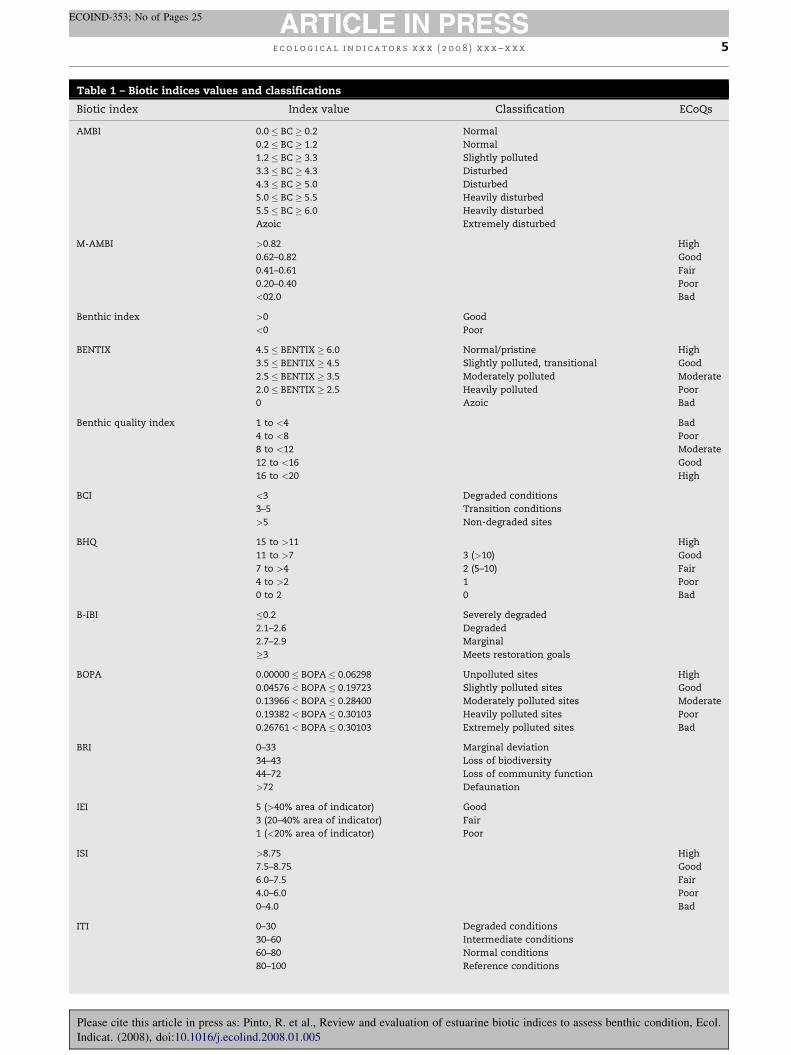
Table 1 – Biotic indices values and classifications

Biotic index Index value Classification ECoQs

AMBI 0.0 � BC � 0.2 Normal

0.2 � BC � 1.2 Normal

1.2 � BC � 3.3 Slightly polluted

3.3 � BC � 4.3 Disturbed

4.3 � BC � 5.0 Disturbed

5.0 � BC � 5.5 Heavily disturbed

5.5 � BC � 6.0 Heavily disturbed

Azoic Extremely disturbed

M-AMBI >0.82 High

0.62–0.82 Good

0.41–0.61 Fair

0.20–0.40 Poor

<02.0 Bad

Benthic index >0 Good

<0 Poor

BENTIX 4.5 � BENTIX � 6.0 Normal/pristine High

3.5 � BENTIX � 4.5 Slightly polluted, transitional Good

2.5 � BENTIX � 3.5 Moderately polluted Moderate

2.0 � BENTIX � 2.5 Heavily polluted Poor

0 Azoic Bad

Benthic quality index 1 to <4 Bad

4 to <8 Poor

8 to <12 Moderate

12 to <16 Good

16 to <20 High

BCI <3 Degraded conditions

3–5 Transition conditions

>5 Non-degraded sites

BHQ 15 to >11 High

11 to >7 3 (>10) Good

7 to >4 2 (5–10) Fair

4 to >2 1 Poor

0 to 2 0 Bad

B-IBI �0.2 Severely degraded

2.1–2.6 Degraded

2.7–2.9 Marginal

�3 Meets restoration goals

BOPA 0.00000 � BOPA � 0.06298 Unpolluted sites High

0.04576 < BOPA � 0.19723 Slightly polluted sites Good

0.13966 < BOPA � 0.28400 Moderately polluted sites Moderate

0.19382 < BOPA � 0.30103 Heavily polluted sites Poor

0.26761 < BOPA � 0.30103 Extremely polluted sites Bad

BRI 0–33 Marginal deviation

34–43 Loss of biodiversity

44–72 Loss of community function

>72 Defaunation

IEI 5 (>40% area of indicator) Good

3 (20–40% area of indicator) Fair

1 (<20% area of indicator) Poor

ISI >8.75 High

7.5–8.75 Good

6.0–7.5 Fair

4.0–6.0 Poor

0–4.0 Bad

ITI 0–30 Degraded conditions

30–60 Intermediate conditions

60–80 Normal conditions

80–100 Reference conditions



Please cite this article in press as: Pinto, R. et al., Review and evaluation of estuarine biotic indices to assess benthic condition, Ecol.



Table 1 (Continued )Biotic index Index value Classification ECoQs

MMI <2 Severe impact

2–6 Patchy impact

>6 No impact

OSI <0 Degraded benthic habitat

0 to <7 Disturbed benthic habitat

7–11 Undisturbed benthic habitat

P-BAT >0.77 High

0.53–0.77 Good

0.41–0.53 Moderate

0.2–0.41 Poor

<0.20 Bad

ECoQs, ecological quality status (sensu WFD).



2.2.2. Multivariate-AMBI, M-AMBI (Muxika et al., 2007)This refined and integrative formula was designed in

response to the WFD requirements to include other metrics

describing the benthic community integrity (e.g. abundance,

biomass or diversity measures) and parameters that are

considered to define better the water bodies’ ecological

quality status (EcoQS). Moreover, it is intended to support

the European Marine Strategy Directive (Borja, 2006), in

assessing the ecological status of continental shelf and

oceanic water bodies (Muxika et al., 2007). The M-AMBI is a

combination of the proportion of ‘disturbance-sensitive

taxa’, through the computation of the AMBI index, species

richness (it uses the total number of species, S), and diversity

through the use of the Shannon–Wiener index, which

overcame the need to use more than one index to evaluate

the overall state and quality of an area (Zettler et al., 2007).

These parameters are integrated through the use of dis-

criminant analysis (DA) and factorial analysis (FA) techni-

ques. This method compares monitoring results with

reference conditions by salinity stretch, for estuarine sys-

tems, in order to derive an ecological quality ratio (EQR).

These final values express the relationship between the

observed values and reference condition values. At ‘high’

status, the reference condition may be regarded as an

optimum where the EQR approaches the value of one. At

‘bad’ status, the EQR approaches the zero value. The M-AMBI

analysis relies on the Euclidean distance ratio between each

area and the reference spots, together with the distance

between high status and bad status reference condition

(Muxika et al., 2007). The stations are located between the

reference conditions and have M-AMBI values ranging from 0

to 1. The boundaries that allow the distinction of the five

ecological states are given in Table 1.

The M-AMBI has been the outcome from the intercalibra-

tion process among states members for the WFD common

methodologies; nevertheless, it has been applied to other

systems outside Europe, like in Chesapeake Bay, USA, where it

revealed to be a consistent measure, providing high agree-

ment percentages with local indices (Borja et al., in press). A

main advantage attributed to this index, as well as of AMBI, is

that both are easily computed, and the software can be freely

downloaded at http://www.azti.es. Moreover, the M-AMBI

seems to provide a more accurate system classification in low



salinity habitats, than the AMBI alone (Muxika et al., 2007;

Borja et al., in press).

2.3. Benthic condition index (Engle and Summers, 1999)

The BCI was designed to evaluate the environmental condition

of degraded systems comparatively to reference situations

(non-degraded conditions) based on the response of benthic

organisms to environmental stressors. This index, which

results from the refinement of a previous attempt (Engle et al.,

1994), reflects the benthic community responses to perturba-

tions in the natural system (Engle, 2000). The benthic index

includes: (1) Shannon–Wiener diversity index adjusted to

salinity; (2) mean abundance for Tubificidae; (3) percentages of

abundance of the class bivalvia; (4) percentages of abundance

of the family Capitellidae; and (5) percentages of abundance of

the order amphipoda.

To calculate this index, one first needs to calculate the

expected Shannon–Wiener diversity index, according to the

bottom salinity:

H0expected ¼ 2:618426� ð0:044795� salinityÞ þ ð0:007278

� salinity2Þ þ ð�0:000119� salinity3Þ (5)

The final Shannon–Wiener’s score is given by dividing the

observed by the expected diversity values. After the calcula-

tion of the abundance and proportions of the organisms

involved, it is necessary to log transform the abundances and

arcsine transform the proportions. Based on this, the

discriminant score is calculated as:

Discriminant score ¼ ð1:5710

� proportion of expected diversityÞ

þ ð�1:0335

�mean abundance of TubificidaeÞ

þ ð�0:5607� percent CapitellidaeÞ

þ ð�0:4470� percent BivalviaÞ

þ ð0:5023� percent AmphipodaÞ(6)


http://www.azti.es/




To turn the index in a practicable and easily understood

measure by policy-makers, the final benthic index score is

given by

Benthic index ¼ discriminant score� �3:217:50

� �� 10 (7)

where �3.21 is the minimum of the discriminant score, and

7.50 is the range of the discriminant score.

When a community is affected by contaminants, the

benthic organisms diminish in abundance and number of

species, while there is an increase in the abundance of

opportunistic or pollution tolerant species. After the discri-

minant score transformation, the benthic index can range

between 0 and 10, being the general scores classifications

presented in Table 1. According to the authors, this index

classifies benthic communities’ condition within and among

estuaries.

2.4. BENTIX (Simboura and Zenetos, 2002)

The BENTIX index was based on the AMBI index (Borja et al.,

2000) and relies on the reduction of macrozoobenthic data

from soft-bottom substrata in three wider ecological groups.

To accomplish this goal, a list of indicators species was

elaborated, where each species received a score, from 1 to 3,

that represented their ecological group. In the light of the

above the groups can be described as:

Group 1 (GI): includes the species that are sensitive or

indifferent to disturbances (k-strategies species);

Group 2 (GII): includes the species that are tolerant and may

increase their densities in case of disturbances, as well as

the second-order opportunistic species (r-strategies spe-

cies);

Group 3 (GIII): includes the first-order opportunistic

species.

The formula that expresses this index is given by

BENTIX ¼ 6�%GIþ 2� ð%GIIþ%GIIIÞ100

� �(8)

This index can range from 2 (poor conditions) to 6 (high

EcoQS or reference sites) (Table 1). Overall, the BENTIX index

considers two major classes of organisms: the sensitive and

the tolerant groups. This classification has the advantage of

reducing the calculation effort while diminishing the prob-

ability of the inclusion of species in inadequate groups

(Simboura and Zenetos, 2002). Moreover, when using this

index, it does not require for amphipoda identification

expertise, since it encloses all those organisms (with exception

to individuals from the Jassa genus) in the same category of

sensitivity to organic matter increasing (Dauvin and Ruellet,

2007). The BENTIX index was developed in the scope of the

WFD for the Mediterranean Sea. It has been successfully

applied to cases of organic pollution (Simboura and Zenetos,

2002; Simboura et al., 2005), oil spills (Zenetos et al., 2004) and

in dumping of particulate metalliferous waste (Simboura et al.,



2007). This index is considered an ecologically relevant biotic

index since it does not under or overestimates the role of any

of the groups (Simboura et al., 2005). Nevertheless, according

to some authors, the BENTIX index relies solely on the

classification of organisms for organic pollution, being unable

to accurately classify sites with toxic contaminations (Marın-

Guirao et al., 2005). It is also emphasized the small lists of

species, especially crustaceans, included in the attribution of

the scores. Another point is that this index presents some

limitations when applied to estuaries and lagoons (Simboura

and Zenetos, 2002; Blanchet et al., 2007).

2.5. Benthic habitat quality (BHQ; Nilsson and Rosenberg,1997)

The benthic habitat quality (BHQ) was designed to evaluate the

environmental condition of the soft-bottom habitat quality of

Havstensfjord (Baltic Sea) through analysis of sediment profile

and surface images (SPIs). The BHQ index relies on the relation

between the classical distribution of benthic infaunal com-

munities in relation to organic enrichment, based on the

Pearson and Rosenberg model (1978). This tool integrates the

structures on the sediment surface, structures in the sedi-

ment, and the redox potential discontinuity (RPD) images.

Therefore, the parameterization of sediment and animal

features may be a useful combination to describe and assess

habitat quality (Rhoads and Germano, 1986). This index

attempts to show the usefulness of sediment profile imaging

in demonstrating benthic habitat changes connected with

physical disturbance, specifically with low oxygen concentra-

tions (Nilsson and Rosenberg, 2000). The calculation of the

BHQ index from the sediment profile images can be computed

by

BHQ ¼X

AþX

Bþ C (9)

where A is the measure of surface structures, B the measure of

the subsurface structures, and C the mean sediment depth of

the apparent RPD. The parameters used in this index were all

measured from the images and the scoring could be seen as an

objective assessment of the successional stages. Deep subsur-

face activity, such as feeding voids and many burrows, which

often is associated with a thick RPD, have a high scoring and

contribute to a high BHQ index. It can range between 0 and 15

(Table 1), where high scores are associated with mature

benthic faunal successional stages and low scores with pio-

neering stages or azoic bottoms. According to Rosenberg et al.

(2004), the BHQ index could also be a useful tool for the WFD

implementation in assessing the BHQ. Therefore, instead of

the earlier separation of the BHQ index into four successional

stages, Rosenberg et al. (2004) underpin the division into five

classes in accordance to the WFD requirements (Table 1).

According to the index authors, this scoring method can be

valid for many boreal and temperate areas, as in these areas

the benthic infauna is similarly structured and has a similar

distribution and activity within the sediment (Pearson and

Rosenberg, 1978; Rhoads and Germano, 1986). Despite sharing

some principles, one main difference that distinguishes these

two indices is that in the organism sediment index (OSI)

(Rhoads and Germano, 1986; see Section 2.15) the successional





stages are determined by examining the images by eye

whereas in the BHQ index the different structures in the

images are scored and their summary relates to a particular

community stage (Nilsson and Rosenberg, 2000).

One advantage enumerated by the BHQ authors is the fact

that a benthic quality assessment based on numerical scoring,

as the one used in the BHQ index, allows statistical

comparisons between strata and communities. Furthermore,

this method can also roughly forecast oxygen regimes over

integrative time scales, becoming a useful tool for environ-

mental managers interested in benthic assessment and in

rough but quantitative approximation of near bottom dis-

solved oxygen regimes (Cicchetti et al., 2006). Moreover, the

use of SPI methods is a rapid and inexpensive way of tracking

and assessing the BHQ, being very useful to characterize the

successional stages of the organic enrichment gradient

(Nilsson and Rosenberg, 2000; Wildish et al., 2003). Never-

theless, according to Wildish et al. (2003) there are some

benthic habitats where this method cannot be applied, as for

example in areas where soft-bottoms are absent and where

coarse sediments or rock predominate; or even in areas where

water depth exceeds reasonable SCUBA diving depths

(approximately 30 m).

2.6. Benthic opportunistic polychaeta amphipoda (BOPA)index (Dauvin and Ruellet, 2007)

The benthic opportunistic polychaeta amphipoda (BOPA)

index results from the refinement of the polychaeta/amphi-

poda ratio (Gomez-Gesteira and Dauvin, 2000), in order to be

applicable under the WFD perspective. Accordingly, this index

can be used to assign estuarine and coastal communities into

five EcoQs categories (Table 1). This index, in accordance with

the taxonomic sufficiency principle, aims to exploit this ratio

to determine the ecological quality, using relative frequencies

([0;1]) rather than abundances ([0;+1]) in order to define the

limits of the index. This way, it can be written as:

BOPA ¼ LogfP

fA þ 1þ 1

� �(10)

where fP is the opportunistic polychaeta frequency (ratio of the

total number of opportunistic polychaeta individuals to the

total number of individuals in the sample); fA is the amphipoda

frequency (ratio of the total number of amphipoda individuals,

excluding the opportunistic Jassa amphipod, to the total num-

ber of individuals in the sample), and fP + fA � 1. Its value can

range between 0 (when fP = 0) and Log 2 (around 0.30103, when

fA = 0). The BOPA index will get a null value only when there

are no opportunistic polychaetes, indicating an area with a

very low amount of organic matter. As so, when the index

presents low values it is considered that the area has a good

environmental quality, with few opportunistic species; and it

increases as increasing organic matter degrades the environ-

ment conditions.

One of the main advantages of this index is its indepen-

dence of sampling protocols, and specifically of mesh sieves

sizes, since it uses frequency data and the proportion of each

category of organisms. The need for taxonomic knowledge is

reduced, which allows a generalised use and ease of



implementation. Moreover, the use of frequencies makes it

independent of the surface unit chosen to express abundances

and it is sensitive to increasing organic matter in sediment as

well as to oil pollution. Nevertheless, it takes into account only

three categories of organisms – opportunistic polychaetes,

amphipods (except Jassa) and other species – but only the first

two have a direct effect on the index calculation. Another

point is that it does not consider the oligochaeta influence,

which may include also opportunistic species.

2.7. Benthic quality index (BQI; Rosenberg et al., 2004)

The benthic quality index (BQI) was designed to assess

environmental quality according to the WFD. Tolerance

scores, abundance, and species diversity factors are used in

its determination. The main objective of this index is to

attribute tolerance scores to the benthic fauna in order to

determine their sensitivity to disturbance. The index is

expressed as:

BQI ¼X Ai

Tot A

� �� ES500:05i

� �� 10LogðSþ 1Þ (11)

where Ai/Tot A is the mean relative abundance of this species,

and ES500.05i the tolerance value of each species, i, found at the

station. This metric corresponds to 5% of the total abundance

of this species within the studied area. Further, the sum is

multiplied by base 10 logarithm for the mean number of

species (S) at the station, as high species diversity is related

to high environmental quality. The goal of using the values

calculated from the 5% lowest abundance of a particular

species (ES500.05) is that this value is assumed to be represen-

tative for the greatest tolerance level for that species along an

increasing gradient of disturbance, i.e. if the stress slightly

increases that species will disappear. This method is similar to

that proposed by Gray and Pearson (1982) and presents the

advantage of reducing the weight of outliers during the index

calculation. This parameter can be computed as:

ES50 ¼ 1�XS

i¼1

ðN�NiÞ!ðN� 50Þ!ðN�Ni � 50Þ!N!

(12)

where N is the total abundance of individuals, Ni is the abun-

dance of the i-th species, and S is the number of species at the

station.

Results from this analysis can range between 0 and 20

(reference value) according to the classification made by the

WFD for the coastal environmental status (Table 1). Two

methodological constrains of this index can be highlighted:

the sample area is not the same among sampling protocols,

and individuals’ distribution among species may not be

random, particularly when some species appear as strong

dominants. Thus, Rosenberg et al. (2004) recommend the use

of many stations and replicates for the quality assessment of

an area. Moreover, according to Zettler et al. (2007) this index

presents strong correlations with environmental variables,

such as salinity, decreasing the scores with decreasing

salinities. Furthermore, this index requires regional datasets

(the ES500.05 calculation is based on the specific framework of

species present at the study-area), and the delimitation of





local reference values, depending on the areas under study

such that different maximum values can be achieved

(Rosenberg et al., 2004; Reiss and Kroncke, 2005; Labrune

et al., 2006; Zettler et al., 2007).

2.8. Benthic response index (BRI; Smith et al., 2001)

The benthic response index (BRI) was developed for the

Southern California coastal shelf and is a marine analogue of

the Hilsenhoff index used in freshwater benthic assessments

(Hilsenhoff, 1987). This index is calculated using a two-step

method in which ordination analysis is employed to establish

a pollution gradient. Afterwards the pollution tolerance of

each species is determined based upon its abundance along

the gradient (Smith et al., 1998). The index main goal is to

establish the abundance-weighted average pollution toler-

ance of the species in a sample, which is considered a very

useful screening tool (Bergen et al., 2000). The basis of this

index is that each species has a tolerance for pollution and if

that tolerance is known for a large set of species, then it is

possible to infer the degree of degradation from species

composition and its tolerances (Gibson et al., 2000). The index

can be given as:

Is ¼Pn

i¼1 piffiffiffiffiffiffiasi

3p

Pni¼1

ffiffiffiffiffiffia f

si3q (13)

where Is is the index value for the sample s, n is the number of

species in the sample s, pi is the tolerance value for species i

(position on the gradient of pollution), and asi is the abundance

of species i in sample s. The exponent f is for transforming the

abundance weights. So, if f = 1, the raw abundance values are

used; if f = 0.5, the square root of the abundances are used; and

if f = 0, Is is the arithmetic value of the pi values greater than

zero, once that all a fsi ¼ 1 (Smith et al., 2001). The average

position for each species (pi) on the pollution gradient defined

in the ordination space is measured as:

pi ¼Pti

j¼1 gi j

ti(14)

where ti is the number of samples to be used in the sum, with

only the highest ti species abundance values included in the

sum. The gij is the position of the species i on the ordination

gradient for sample j. The pi values obtained in Eq. (14) are used

as pollution tolerance scores in Eq. (13) to compute the index

values.

This index provides a quantitative scale ranging from 0 to

100, where low scores are indicative of healthier benthic

communities (i.e. community composition most similar to

that occurring at unimpacted regional reference sites). The BRI

scoring defines four levels of response beyond reference

condition (Table 1). Although it can be useful to quantify

disturbances, it is not able to distinguish between natural and

anthropogenic disturbance, such as the natural impacts that

river flows may have on benthic communities (Bergen et al.,

2000). Nevertheless, this index presents the advantage of not

underestimating biological effects, as well as presenting low

seasonal variability (Smith et al., 2001).



2.9. Biological quality index (BQI; Jeffrey et al., 1985)

The biological quality index (BQI) is based on biosedimentary

communities (Wilson, 2003), such as Scrobicularia plana,

Macoma balthica, and Hediste diversicolor. This index detects

pollution in estuaries, although there are some problems in

the detection of the pollution status between that of stable

communities and abiotic environments. A number of

approaches have been tried in the marine environment.

These include the use of the log-normal distribution (Gray,

1979) and the use of diversity indices such as the Shannon–

Weiner or indicator species (Eagle and Rees, 1973). The index is

given by

BQI ¼ antilog10ðC�AÞ (15)

where C is the proportional biological area and A is the pro-

portional abiotic area. A + B + C = 1.0, where B is the opportu-

nistic.

The estuary BQI is obtained by the addition of each zone

BQI multiplied by the proportional area of their respective

zones. The index can range from 0.1 (completely abiotic) to a

maximum of 10 (completely unpolluted). This classification

was based on the communities’ division into abiotic (with-

out macrobiota), opportunistic, or stable (biological com-

munities usually present in that kind of substrate; Wilson,

2003). Although, it gives a rapid and effective overview, it

does not offer a complex discrimination of a system (Wilson,

2003).

2.10. Index of biotic integrity complex

Many variations of IBI (Karr, 1991) have been developed for

freshwater systems. This index design has been adapted and

applied to several other systems, such as terrestrial environ-

ments, lacustrine systems, estuaries or coral reefs, using a

wide range of metrics that better characterize the system

under study, such as macroinvertebrates (e.g. Weisberg et al.,

1997), fishes (e.g. Deegan et al., 1997), or coral reefs (e.g.

Jameson et al., 2001). Indices like the Chesapeake Bay B-IBI

(Weisberg et al., 1997) or the macroinvertebrate index of biotic

integrity (mIBI) (Carr and Gaston, 2002) are examples of

ecological measures that try to integrate several features and

characteristics of a particular system in order to evaluate its

condition, using for it the study of the benthic communities

present in the system. These two indices are designed to

evaluate the ecological health of an estuary.

2.10.1. Benthic index of biotic integrity (Weisberg et al., 1997)

The Chesapeake Bay B-IBI (Weisberg et al., 1997) integrates

several benthic attributes, related to healthy benthic com-

munity structure, in order to calculate the global condition of a

region. It gives the actual status of the benthic community as a

function of its deviation from the reference condition.

Therefore it can provide trends within the system once

calibrated to reference conditions. The indicators used to

calculate the benthic index are: (1) Shannon–Wiener species

diversity index; (2) total species abundance; (3) total species

biomass; (3) percent abundance of pollution indicative taxa; (4)

percent abundance of pollution sensitive taxa; (5) percent





biomass of pollution indicative taxa; (6) percent biomass of

pollution sensitive taxa; (7) percent abundance of carnivore

and omnivore species; (8) percent abundance of deep-deposit

feeders; (9) tolerance score and (10) Tanipodinae to Chirono-

midae percent abundance ratio.

To calculate the index metrics several steps have to be

implemented (Llanso, 2002). The epifaunal species have to be

eliminated from the species lists and from the calculation, as

well as other individuals that are not representative of the

subtidal communities (e.g. Nematoda or fish species). To

calculate the diversity measure (H0), higher taxonomic groups

have to be retained as well (e.g. polychaeta or amphipoda). The

sensitive/indicative pollution species can be classified accord-

ing to the AMBI species classification, considering the I and II

ecological groups as sensitive to pollution and the ecological

groups IV and V as pollution indicative species. When field and

experimental data are not available for feeding strategies

metrics (% of carnivore–omnivore species and % subsurface

deposit feeders), a literature review can be made in order to

classify all the catched species.

Although the B-IBI index integrates eleven metrics, not all

of them are used here to calculate the overall ecosystem

score and condition. Llanso et al. (2002a) defined seven

major estuarine stretches for the Chesapeake Bay, according

to the Venice transitional water organization scheme for

salinity and sediment types. Depending on the estuarine

stretch under analysis, different metrics are used to

estimate the local condition and status (Table 2). Moreover,

the tolerance score and the percentage of Tanipodinae to

Chironomidae metrics were considered by the index authors

as facultative, as long as no score was attributed to them and

that, for the oligohaline zone, the lack of the two metrics

was considered in the index average calculation (removed

from the denominator factor). This index classification gives

scores for the different indicators in relation to the reference

conditions. When the two situations are identical, a score of

5 is given and when they are very different a score of 1 is

attributed. The final index score is determined by the

average of the individual scores (Llanso et al., 2002b).

Table 1 gives the final classification of the benthic commu-

nity condition.

Other indices have been developed having the B-IBI as a

role model, nevertheless adapted for other geographical

systems (e.g. Van Dolah et al., 1999).

Table 2 – Metrics used to calculate the final B-IBI scores accor

Euhalineestuarine

Polyhmud

Shannon–Wiener diversity measure � �Total species abundance � �Total species biomass � �% Abundance pollution indicative sp.

% Biomass pollution indicative sp. � �% Abundance pollution sensitive sp. �% Biomass pollution sensitive sp. �% Carnivore-omnivore sp. �% SsDF sp. �% Tanipodinae to Chironomidae

Tolerance score



2.10.2. Macroinvertebrate index of biotic integrity (Carr andGaston, 2002)The mIBI is a multimetric index that was designed to evaluate

the benthic condition of an ecosystem, and was developed

specifically for application to the Calcasieu estuary (USA). The

index is composed of four metrics: (1) abundance of pollution

sensitive organisms (ranked in a decreasing order); (2)

abundance of pollution tolerant organisms (ranked in an

increasing order); (3) total abundance and (4) species diversity.

The indicator species considered are based on the work of

Rakocinski et al. (1997) that divided the species into categories

of pollution tolerant or pollution sensitive. After summing

each metric for each site, the scores are ranked and normal-

ized. The metric data are normalized with the attribution of

scores to accurately weight of the metrics in the index. This

was achieved by using the rank-normalized data in order to

provide a better precision for data analysis and to avoid the

distribution of the data. In the end, the index classification

falls within a scale of 0 (worst conditions) to 1 (best

conditions).

2.11. Indicator species index (ISI; Rygg, 2002)

The indicator species index (ISI), that is based on the improved

version of the Hurlbert index (1971), focuses on the assump-

tion that each species reacts differently to pollution impacts,

and consequently to the degradation of the ecosystem

conditions. Knowing the species sensitivity to pollution

factors, their presence or absence can be used to calculate

the ISI in each sample (it does not enter with taxa abundance).

To calculate this index it is necessary to determine the

sensitive values for each species as well as the pollution

impact factor (ES100min5). The ES100 is the expected number

of species among 100 individuals. The average of the five

lowest ES100 was defined as the sensitivity value of that taxon,

denoted ES100min5. The ISI is then defined as the average of

the sensitivity values of the taxa occurring in the sample. This

index allows an accurate description of environmental quality

of the systems and has been applied mostly in the Norway

coasts.

One main disadvantage of the ISI is that it may not be

transposed to other geographical regions without restrictions,

since the taxonomic list can be significantly different and the

calculation of the sensitivity factors may require different

ding to estuarine zones

alinedy

Polyhalinesand

Mesohaline Oligohaline

� ��

� ��

� ��

��





approaches. Table 1 provides the ranges of classification in

accordance to the WFD requirements.

2.12. Index of environmental integrity (IEI; Paul, 2003)

The index of environmental integrity (IEI) was developed to

assess the overall condition of a region and was first used in the

Mid-Atlantic region. This index is based on the evaluation of

signals derived from natural or anthropogenic sources given by

the natural systems. These signals are then used to identify the

condition of the system and the causes that provoked it. The IEI

final value is obtained through the integration of the weighted

average of individual subindex values, which is given as:

IEI ¼Pn wiIiPn wi

(16)

where wi is the weight for the subindex i, Ii is the value for the

subindex i; and n the number of subindex values.

To establish the final classification, values were assigned to

each parameter for each area according to the percent area for

the indicator (Table 1). When applying this index it must be

considered that it was based on a restricted number of

indicators.

2.13. Infaunal trophic index (ITI; Word, 1978)

The infaunal trophic index (ITI) was initially designed to

identify degraded environmental conditions caused by

organic pollution along the California coasts. This index, a

numeric representation of the relative abundance of the

dominant infaunal organisms, is based on the distribution of

the macrozoobenthos species according with their trophic

category. The ITI draws on the premise that the community

structure can be evaluated by the feeding behaviour of the

benthic invertebrates as a response to the organic matter

content in the sediment or water column. There are four main

organisms’ categories (Word, 1980):

(1) suspension detritus feeders (such as the polychaete Owenia

sp.);

(2) interface detritus feeders (as the polychaete Glycera sp.);

(3) surface deposit feeders (like Hediste or Hinia species); and

(4) subsurface deposit feeders (e.g. Capitella capitata or oligo-

chaeta species).

With this division of the organisms in a sample, the trophic

structure can be calculated using the formula:

ITI ¼ 100� 33:33� 0� n1 þ 1� n2 þ 2� n3 þ 3� n4

n1 þ n2 þ n3 þ n4

� �(17)

where n1, n2, n3, n4 are the number of individuals sampled in

each of the above mentioned groups. The coefficient in the

formula (0–3) is a scaling factor that allows the index to range

gradually between 0 and 100 and to be sensitive to changes in

infaunal feeding strategies. Word (1978) established that values

near 100 are indicative of a majority of suspension feeders,

which means that the environment is not disturbed. Values

near 0 are indicative of a subsurface deposit feeder’s domi-

nance, meaning that the environment is degraded (Table 1).



One of the disadvantages is the difficulty in determining the

organism’s diet and thus attributing it to a particular trophic

level. Generally, the diet, which can be observed in the stomach

content or in laboratory experiments, is difficult to establish,

and can vary from one population to another among the same

taxonomic group. Moreover, due to geographical restrictions,

the feeding behaviour of certain species can be largely influ-

enced by their habitat conditions. For example, Caprella sp.

along the European coast is considered a predator (Mancinelli

et al., 1998), whereas along the American coasts exhibits sus-

pension feeding behaviour (Word, 1990).

This index has been applied to systems such as bays

(Donath-Hernandez and Loya-Salinas, 1989) with reasonably

satisfactory results. It is also important to state that ITI has a

limited sensitivity to changes in abiotic and biotic components

and it is not a good descriptor of system health (Maurer et al.,

1999). It also presents limitations when comparisons between

different geographic areas are done, since each ecosystem has

its own dominant local species, which requires a specific

feeding behaviour and scaling factor. The ITI index was

recommended as an assessment tool for monitoring programs

and it is widely used as a pollution index (Kennish, 1997). It can

also be a very useful tool in management decisions (Maurer

et al., 1999), although its use should suffer a critical approach.

2.14. Macrofauna monitoring index (MMI; Roberts et al.,1998)

The main goal of the macrofauna monitoring index (MMI) is

assessing the impact of dredge oil dumping, based on

monitoring indicator species in the benthic macrofauna. It

is based on twelve indicator species, according to the criteria

of easiness of identification, easy extraction from samples,

and representativeness. Each species was rated from 1 to 10

(very intolerant to impacts) based on the density of species in

control versus impacted sites. A score of 0 indicates a species,

which is more common at impacted samples than at

unimpacted sites. This score reflects basically the impacts

that dredge spoil dumping have on its abundance. The index

final score (Table 1) was obtained by the averaged sum of all

the species scores. Its aim was the development of a site-

specific monitoring index that would be statistically precise,

biologically meaningful and very cost effective.

According to Roberts et al. (1998), the impacted sites show a

higher content in mud or fine sand presenting lower macro-

faunal abundance, diversity, and richness than the unimpacted

regions. This index identifies and estimates the stress and

disturbance on the study site without appealing to exhaustive

identification methods, since it relies on a small but informative

subset of fauna.The MMIpresentstwomaindisadvantages: this

index is semi-quantitative measure of the degree of impact on

macrofauna, correlating strongly with macrofaunal richness

and abundance (Roberts et al., 1998) and it is site and pollution

type specific (Simboura and Zenetos, 2002).

2.15. Organism sediment index (Rhoads and Germano,1986)

The OSI was developed to assess the BHQ in shallow water

environments, allowing the evaluation of stages of organic





pollution in the ecosystem. This index presents four main

metrics (1) dissolved oxygen conditions; (2) depth of the

apparent RPD; (3) infaunal successional stage; and (4) presence

or absence of sedimentary methane. The successional stage

was measured with sediment profile images, which char-

acterizes the benthic habitat in relation to physical–chemical

features (Rhoads and Germano, 1982). The OSI index has also

been used in some studies to map habitat quality (Rhoads and

Germano, 1986), to assess physical disturbances and organic

enrichment (Valente et al., 1992), and to evaluate the effects of

mariculture (O’Connor et al., 1989). Two recent studies showed

that low values of apparent RPD were correlated with low OSI

scores (Nilsson and Rosenberg, 2000).

Rhoads and Germano (1986) based their index on mean

depth of the apparent RPD, the presence of gas voids, and on a

visual classification of the infauna into successional stages,

which could range from �10 to +11. The lowest values are

attributed to the bottom sediments with low or no dissolved

oxygen, without apparent macrofauna, and with methane

present in the sediment. The highest values are attributed to

aerobic sediments with a deep apparent RDP, established

macrofaunal communities, and without methane gas. The

index classification is provided on Table 1.

2.16. Portuguese-benthic assessment tool

The P-BAT integrates, in a cumulative index, three widely used

metrics – Shannon–Wiener index (H0), Margalef index (d) and

AMBI – which are based on different approaches when

evaluating system status. This integration results from

experience works on the Portuguese transitional and coastal

waters systems that demonstrate that, when evaluating the

system condition, the combination of several metrics is more

accurate than single metrics. The Shannon–Wiener index is a

diversity measure that takes into account the proportional

abundance of species; the Margalef index is based on the

specific richness of a system and the AMBI on the ecological

strategies followed by estuarine organisms (indicator species).

Overall index classifications have been developed for the

Portuguese transitional water bodies (Table 1), in order to be

integrated in the WFD as a reference measure (Teixeira et al.,

personal communication) and it can range between 0 (bad

ecological quality) and 1 (good ecological quality).

To calculate the multimetric approach, the Shannon–

Wiener, Margalef and AMBI values (previously calculated)

were standardized by subtracting the mean and dividing by

the standard deviation. Afterwards, a FA was conducted to

construct a three coordinate system that was then used to

derive the final station score, using as comparison the

reference conditions determined for the system. These

reference conditions were estimated based on two opposite

situations: the best condition that a system could present

Benthic index ¼ 1:389� ðsalinity normalized Gleason0s; D; base28:4� 0

� salinity normalized Tubificidae abunda119� 0:375

¼ 0:0489� salinity normalized Gleason0s;D

normalized Tubificidae abundance� Spio



(without impacts) versus the worse possible scenario for the

same system (Bald et al., 2005; Muxika et al., 2007). The P-BAT

index was developed with data from the Mondego estuary

(Portugal) for winter conditions and using a 1 mm sieve.

2.17. Pollution load index (PLI; Jeffrey et al., 1985)

This index, based on contaminations loads, includes three

parameters: (1) water; (2) fauna; (3) flora and sediment. The PLI

scores individual sediment contaminants according to a log

scale from baseline to threshold (Wilson, 2003). The formula is

computed as:

PLI ¼ antilog10 1� CP� BT� B

� �� (18)

where CP is the pollutant concentration; B the baseline, unpol-

luted; and T the threshold, damage. The scores for each

pollutant are summed to give a total site PLI thus,

Site PLI ¼ ðPLI1 � PLI2 � PLInÞ1=n; for n pollutants (19)

The sites scores are then summed likewise to give the

estuary index value:

PLI ¼ ðPLI1 � PLI2 � PLI jÞ1= j; for j sites (20)

The PLI varies from 10 (unpolluted) to 0 (highly polluted).

This index allows the comparison between several estuarine

systems and has been applied in several geographical regions,

like in Europe and US estuaries (Wilson, 2003). Caeiro et al.

(2005) have highlighted the ease of implementation of this

index.

2.18. Virginia province benthic index (VPBI; Paul et al.,2001)

This benthic index has been developed over two stages for

application in the Virginia province, USA. Here we detail the

most recent formulation by Paul et al. (2001) which is an

expanded version of Schimmel et al. (1999). The goal of VPBI is

to evaluate the benthic condition of estuarine communities,

discriminating between degraded and non-degraded sites.

This index is based on a measure of diversity (related with

unimpacted sites) and the abundance of pollution tolerant

taxa, Tubificidae, and Spionidae (related with impacted

conditions). The index was developed for the U.S. EPA

Environmental Monitoring and Assessment Program. The

three benthic metrics in the index are: 1) salinity normalized

Gleason’s, D, based upon infauna and epifauna; 2) salinity

normalized Tubificidae abundance; and 3) abundance of

Spionidae. This index is given by:

d upon infauna and epifauna� 51:5Þ:651

nce� 28:2�ðSpionidae abundance� 20:0Þ45:4

� 0:00545� salinity

nidae abundance� 2:20

(21)





where salinity normalized Gleason’s, D, based upon infauna

and epifauna = Gleason’s D/(4.283 � 0.498 � bottom salini-

ty + 0.0542� bottom salinity2 � 0.00103 � bottom salinity3)

� 100 and salinity normalized Tubificidae abundance = Tubi-

ficidae abundance � 500 � exp(�15 � bottom salinity), and

exp(. . .) denotes the exponential function.

The salinity normalization for Tubificidae abundance

required a different procedure than that used to normalize

the other benthic metrics. Tubificidae are only observed for

low salinity water with some occurrence being normal for

unimpacted sites. Impacted sites would be characterized by

large Tubificidae abundances. This index identifies the

unimpacted sites by a negative gradient of salinity normalized

abundance and the impacted sites with positive values. In this

index, positive values are indicative of healthy community

conditions and negative values reflect degraded communities

(Table 1).

Although this index gives an overall system condition, it is

important to notice that it was based on the benthic

communities, so the habitat condition of the pelagic area,

submerged aquatic vegetation and marshes is not assessed.

3. Application of three broadly used indices:the Mondego estuary case study

3.1. Study site: Mondego estuary

The Mondego estuary, located on the western coast of Portugal

(408080N, 88500W), is a warm temperate estuary with about

21 km long. In its terminal part the estuary is composed by two

branches – North and South arms – separated by an alluvium-

formed island (Morraceira Island) (Fig. 1). These two sub-

systems present distinct hydrological characteristics. The

North arm is deeper (5–10 m during high tide), presents

stronger daily salinity changes (the freshwater flows basically

through this arm), and the bottom sediments consist mainly of

medium to coarse sand (Marques et al., 1993). This estuarine

branch constitutes the principal navigation channel, support-

ing the harbour and city of Figueira da Foz, and is subject to

Fig. 1 – Sampling stations used in the Mondego estuary subtidal

5–9; polyhaline sand: 11–16; mesohaline: 17–19 and oligohaline



constant dredging activities. On the other hand, the South arm

is shallower (2–4 m during high tide), is composed mostly by

sand to muddy bottoms, and until recently was almost silted

up in the upstream connection to the main river course. This

constraint forced the water circulation to be mainly depen-

dent on tidal penetration and the freshwater inflow of a

tributary, Pranto River, controlled by a sluice (Marques et al.,

1993; Patrıcio et al., 2004). All these factors contribute to the

strong daily temperature oscillations verified in this sub-

system.

The entire estuary is under permanent anthropogenic

pressures and several impacts determine its maintenance and

development as a system (Marques et al., 2003). From 1997

onwards, experimental mitigation measures have been

applied attempting to reduce the eutrophication symptoms

in the South arm (e.g. Zostera noltii beds decline).

According to Teixeira et al. (in press) with the division of the

Mondego estuary by stretches, the entire natural variability/

diversity within this system should be covered. Apart from

salinity features (based on the Venice symposium classifica-

tion) different habitats that might provide different possibi-

lities for benthos to settle are accounted for. Five major

stretches were considered (Fig. 1): the euhaline estuarine

stretch, located near the estuary mouth and characterized by

high bottom salinities; the polyhaline muddy area (with a

mean bottom salinity of 27 and with similar communities

features, influenced by sediment type); the polyhaline sand

zone, located in the North arm; the mesohaline stretch, with a

mean salinity of 14 and the oligohaline stretch (bottom salinity

of 1.7). Moreover, in the Mondego estuary, the Southern and

Northern arms have been described as two different sub-

systems (Marques et al., 1993, 2003), where the North arm has

been considered as possessing benthic communities’ impov-

erishments relative to the South arm, mainly due the higher

sediment instability (Marques et al., 1993).

3.2. Sampling and laboratorial procedures

In August 2005, as part of the Mondego estuary survey,

subtidal soft-bottom macrofauna were sampled at 25 stations

survey. Euhaline estuarine: 1–4 and 10; polyhaline muddy:

: 20–25.





along the estuary (Fig. 1). Five replicate samples were

randomly collected, at each station, using a van Veen LGM

grab, with 0.078 m2 dredging area, immediately sieved through

sieve-screen with a 0.5 mm mesh, and preserved within a 4%

formalin solution. In the laboratory samples were washed

through a series of nested sieves of 1.0 and 0.5 mm, sorted and

identified to the lowest possible category, preferentially to

species level. Once identified and counted, biomass was

estimated as ash free dry weight (g AFDW m�2) by drying to

constant weight at 60 8C and ashing at 450 8C for 8 h.

In conjunction with the macrofaunal sampling, salinity,

temperature, pH and dissolved oxygen were measured in situ

at each station to accurately characterize the overall ecosys-

tem’s condition. For chlorophyll a and total suspended solids

(TSSs) measurements, a bottle of water was collected, and

afterwards filtered. Analogously, a separate sediment sample

was also colleted, where the organic matter content and grain

size were estimated. Winter 2005 sediment samples and

salinity data were considered to determine the stretches

patterns consistency.

At the laboratory, chlorophyll a (mg Chl a m�3) was

determined following the Strickland and Parsons (1972)

method. The organic matter was estimated as the difference

between the dry sediment sample (dried at 60 8C during 72 h)

and the sediment weight after its combustion (450 8C for 8 h).

The sediment type was determined by mechanical separation

in a continuous sieve column after organic matter content

removal. The Brown and McLachland (1990) classification

system (clay: <0.038 mm; silt: >0.038 to <0.125 mm; fine sand:

>0.125 to <0.250 mm; mean sand: >0.250 to <0.500 mm;

coarse sand: >0.500 mm) was followed and the final results

were presented as the percentage of that sediment class in the

total weight of the sample.

3.3. Indices general considerations

In order to evaluate the condition and integrity of the Mondego

estuary, two indices were tested – BCI (see Section 2.3 and

Table 1; Engle and Summers, 1999) and B-IBI (see Section 2.10.1

and Table 1; Weisberg et al., 1997) – and afterwards compared

with the P-BAT (see Section 2.16 and Table 1), developed in the

scope of WFD, in order to compare with the two other

combinative indices scores. It is important to highlight that for

the B-IBI application, the estuarine system had to be divided

into stretches (Llanso, 2002). Teixeira et al. (in press) applied

the same principles to the Mondego estuary, achieving five

major areas within the estuary (euhaline estuarine, polyhaline

muddy, polyhaline sand, mesohaline and oligohaline). The

Llanso metrics attribution scheme was applied to most of the

Mondego estuary ecosystems; however, the authors did not

Table 3 – Indices final classifications correspondence: Portuguindex and benthic index of biotic integrity (B-IBI)



considered the euhaline estuarine ecosystem. The metrics and

score ranges for the polyhaline sand system were used since

they presented the same salinity and sediment types

classifications (Table 2). The tolerance score and the percen-

tage of Tanipodinae to Chironomidae metrics could not be

applied to this case study due to the lack of information

regarding the pollution tolerance capacity for most of the

species. Moreover, in our data set, the Chironomidae species

were all considered as a general group and were not separated.

3.4. Data analysis

One-way ANOVA tests were used to evaluate differences of the

two sieve mesh sizes (combined 1 mm + 0.5 mm and 1 mm

alone) in characterizing the Mondego estuary benthic com-

munities. Differences were evaluated for the several mea-

sured indices along the estuarine systems. The Pearson

correlation analysis was calculated to evaluate the association

between the several BCI parameters and the environmental

variables observed in summer conditions. The environmental

data (physical–chemical parameters) were previously log

transformed (Log(X + 1)) before its use to reduce heterogeneity

in variance.

SIMPER analysis was undertaken (PRIMER 5.2.6# software

package from Plymouth Marine Laboratory, UK), considering

the entire estuarine system and the five salinity stretches

defined for the Mondego estuary, in order to recognize the

species allocation along the distinct estuarine habitats.

Finally, a kappa statistic was used to compare the

qualitative classifications obtained by the different indices.

The kappa coefficient is a widely used indicator of categorical

agreement measure. This test has as main goal the assess-

ment of the agreement on multicategory rating by two

measures, classifying a sample on the same categorical scale.

In order to achieve this, a square table is necessary to

formulate. It was then followed the Landis and Koch (1977)

classification ranges.

In order to compare the indices, a correspondence had to be

made previously between the final score’s classifications

(Table 3).

4. Results

4.1. Mesh size

The density values (ind. m�2) were significantly higher for the

combined (1 mm + 0.5 mm) sieve (ANOVA, F = 6.87, p = 0.0117).

This sieve presented a density almost 64% higher than the

1 mm sieve. Regarding the number of taxa, significantly higher

ese-benthic assessment tool (P-BAT), benthic condition





values were also found in the combined sieve (ANOVA,

F = 9.38, p = 0.004).

Furthermore, analysis of the density results revealed

higher differences between sieves in the upstream stations

(Fig. 2A), while the number of taxa presented the opposite

behaviour, with stronger disparities near the mouth and in the

South arm of the estuary (Fig. 2B). Total biomass values were

not significantly different between sieves (ANOVA, F = 0.00,

p = 0.99) probably because only very small individuals are

retained with the 0.5 mm mesh screen (Fig. 2C). The retention

of large and weighty individuals (e.g. green crab Carcinus

maenas or bivalvia species as Cerastoderma edule and Corbicula

fluminea), as well as of key species like the Isopoda Cyathura

carinata and the gastropoda Hydrobia ulvae, provided a

Fig. 2 – Macrofaunal density (A), number of taxa (B), and macrof

(1 mm + 0.5 mm), along 25 estuarine stations, in summer 2005.



balanced relation for the loss of the abundant but tiny

individuals captured by the 0.5 mm screen. In August 2005,

the subtidal communities appear to be relatively diverse and

moderately abundant in the main river course (North arm).

Despite presenting lower density values, the stretches

corresponding to the South arm and estuary mouth showed

higher number of species (taxa), suggesting a more balanced

community structure (Table 4).

To obtain a full understanding of the differences between

sieves a retention efficiency rate was calculated. Retention

efficiency is the proportion of organisms retained in the 1 mm

sieve compared with the densities found in the combined

sieve (Schlacher and Wooldridge, 1996). At species level,

sieving losses were especially notorious for all species usually

auna biomass (C) using the 1 mm and the combined sieves



Table 4 – Number of taxa and mean (Wstandard deviation) species density (ind. mS2) in the estuarine stretches, in summer2005

Sieve

1 mm Combined

No. of taxa Density No. of taxa Density

Euhaline estuarine 51 24.3 (�45) 104 31.8 (�78.7)

Polyhaline muddy 28 63.9 (�147.9) 51 68.1 (�163.8)

Polyhaline sand 40 266.4 (�662.3) 57 518.7 (�1950.6)

Mesohaline 22 239.7 (�620.3) 35 475.2 (�2000.8)

Oligohaline 15 422.7 (�942.8) 29 564.9 (�1558.2)

Total estuary 81 312.3 (�963) 145 478.3 (�2364.4)



highly abundant in subtidal ecosystems, such as polychaeta

(e.g. Autolytus sp., Mysta picta,), amphipoda (e.g. Atylus falcatus,

Pontocrates altamarinus), and small Isopoda species (e.g.

Zenobiana prismatica). Regarding this, retention efficiency rate

was calculated for the 1 mm sieve considering higher

taxonomic groups (polychaeta, bivalvia, amphipoda, deca-

poda, isopoda, gastropoda, oligochaeta, other crustacea, other

groups). The density values of the two sieves fractions were

compared through a one-way ANOVA analysis. This test

revealed that only the polychaeta and bivalvia groups were

significantly underestimated and presented significant losses

between the two sieves (ANOVAPoly, F = 4.10, p = 0.0486;

ANOVABiv, F = 5.32, p = 0.0254). Analysing the density patterns

in the two sieves, visible changes in the community structure

composition were verified. This trend can be partially

explained by the low retention capacity of juvenile forms

and smaller organisms using the 1 mm sieve alone. For

example, half of the total bivalvia density was lost with the

Table 5 – Benthic condition index (BCI), benthic index of bioticBAT) final scores and classifications, using the two sieves (1 msummer 2005 (white: non-degraded; grey: moderate; and blac



1 mm sieve, mainly due to the juveniles’ forms of C. glaucum, S.

plana, and C. fluminea.

4.2. P-BAT

The main goal of applying this methodology in the present

work was to use this metric value as a reference classification

to validate the results obtained by the two tested indices (BCI

and B-IBI). Analysing the P-BAT final results, using both sieves,

was possible to observe that there were some classification

disparities. According to this index, the final estuarine

condition assessment ranged between Moderate and High

classifications in both sieves. In the 1 mm sieve 92% of the

stations presented a High or Good ecological status. This value

suffered a slight decrease for the combined sieve, where 16%

of the stations presented Moderate conditions. The classifica-

tion differences observed for both sieves were near 30%,

corresponding to 7 stations from a total of 25 (Table 5) (Fig. 3).

integrity (B-IBI), Portuguese-benthic assessment tool (P-m and combined sieves), along the 25 estuarine station, ink: degraded)



Fig. 3 – P-BAT performance for the 1 mm and the combined sieves in summer 2005.



4.3. Benthic condition index

The five BCI metrics (Shannon–Wiener diversity index

adjusted to salinity, mean Tubificidae abundance and Capi-

tellidae, bivalvia and amphipoda percents) were individually

calculated and integrated in Eq. (6) in order to calculate the

overall index score for each station, using two different

density data sets: the 1 mm mesh screen and the combined

sieve (Table 5). In the Mondego estuary, using the 1 mm sieve,

the BCI ranged between�0.78 and 9.5. The higher values were

achieved mainly by the euhaline estuarine stations (except

station 10), the mesohaline (except station 18) and two

oligohaline stations (21 and 22). In summary, 24% (six stations)

of the stations were classified as degraded and 36% (nine

stations) as non-degraded.

In the combined sieve the values presented a variation

between 1.13 and 9.66. Using this sieve, eight stations were

classified as non-degraded: two in the South arm (polyhaline

muddy stretch) (stations 7 and 9), three of the oligohaline

stretch (20–22) and three of the euhaline estuarine (1, 2 and 4).

Table 6 – Significant Pearson correlation coefficients between thparameters, using the 1 mm and combined sieves (N = 25; p <

Environmental variables

BCI H0 Tubifi

Comb 1 mm Comb 1 mm Comb

pH

Salinity �0.42

O2 (%) �0.40

Chl a (mg m�3)

SST

POM �0.51

Coarse sand (%)

Medium sand (%)

Fine sand (%) 0.66* 0.41

Silt (%)

Clay (%)

Organic matter (%)



As so, 36% (9) of the stations were classified as degraded, while

32% (8) presented a good environmental quality.

Comparing the index performance between the sieves

final classifications, some changes are perceived since 48%

of the final index scores were not consistent (12 stations).

The differences between the two sieves were noticeable and

there were two cases where the given classification was

extreme, in stations 3 and 17, classified as non-degraded by

the 1 mm sieve and as degraded by the combined sieve.

From an overall perspective better system conditions were

achieved using the 1 mm sieve alone. Nineteen stations

were considered as having good or moderate status, while

with the combined sieve there were 16 stations with the

same classification.

Correlation analyses were performed in order to evaluate

the index submetrics that suffered greater influence from

the environmental variables (Table 6). Some differences were

found analysing the relation between individual metrics in the

two sieves and environmental variables. These differences

were mainly in the percent of Capitellidae and bivalvia

e benthic condition index (BCI) metrics and environmental0.05; *p < 0.01), in summer 2005

BCI

cidae Amphipoda Capitellidae Bivalvia

1 mm Comb 1 mm Comb 1 mm Comb 1 mm

�0.55 �0.43 �0.43 �0.48

�0.41

0.63* 0.64*

�0.46 �0.47 0.70*

�0.45

0.62*

0.83*

0.74*

0.88*





associated with environmental factors. Using the combined

sieve, it was possible to observe that there was a strong

positive correlation between sediment type and its organic

matter content and the abundance of Capitellidae. This

relation was not captured when using the 1 mm mesh screen

alone. Although the original benthic index components were

not correlated with salinity (the only factor correlated was the

diversity index and it was adjusted to this variable deviation in

the index development), this was not verified for the Mondego

estuary. In this case study, three variables were naturally

correlated with salinity (Tubificidae abundance and amphi-

poda percent in both sieves, and bivalvia percent in the

combined sieve). All the other index submetrics did not

present significant correlations with environmental para-

meters. In the Mondego estuary there were several factors

significantly correlated with natural variables mainly with the

combined sieve.

4.4. Benthic index of biotic integrity

The B-IBI results were obtained through the adequate

scoring criteria average, according to the estuarine area

under study (Table 5). Accordingly, the values for the

combined sieve ranged between 1.7 and 3.5. 36% of the

Mondego estuary stations were considered as severely

degraded, 40% as degraded, and only 24% as meeting

restoration goals or marginal (4 and 2, respectively). Never-

theless, the index performance was also tested using the

1 mm sieve alone and the B-IBI presented values between 1.7

and 4, classifying 28% of the stations as severely degraded,

44% as degraded, 8% as marginal, and 20% as meeting

restoration goals.

Through sieve comparison, 28% of the stations (corre-

sponding to seven stations) showed dissimilarities in the

final B-IBI classifications. The polyhaline sand stretch was

the estuarine zone that presented a higher classification

consistency within sieves, with all the stations presenting

the same classification. In contrast, the polyhaline muddy

was the estuarine area that presented higher differences

between sieves, where three stations from five, presented

dissimilar classifications. At station 18, opposite conditions

were achieved, being classified as non-degraded by the

1 mm sieve whereas the combined sieve provided a

degraded status.

Table 7 – Kappa analysis coefficients for the indices applied toclassification, following Landis and Koch (1977) classificationcondition index; B-IBI, benthic index of biotic integrity)

Kappa coefficient

Sieves comparison P-BAT sieves 0.448

BCI sieves 0.284

B-IBI sieves 0.591

1 mm sieve P-BAT-B-IBI 0.002

P-BAT-BCI 0.124

B-IBI-BCI 0.058

Combined sieve P-BAT-B-IBI �0.042

P-BAT-BCI 0.107

B-IBI-BCI 0.084



4.5. Biotic indices comparative approach

The samples were sieved through two sizes of meshes to

determine the effect of sieve size on the indices final scores

and classifications. At station 3, worse environmental condi-

tions are observed when using the combined sieve with the P-

BAT and benthic index. Nevertheless, this change was not

captured by the B-IBI. The SIMPER analysis concerning this

station showed that 90% of the community density is attained

by two species: Pisione remota and Glycera trydactila. Even so,

and despite the 58.5% dissimilarity average between sieves, it

was not possible to determine the discriminant species, due to

the low number of replicates. The effect of screen size on

sampling variability was not statistically significant for all

tested indices (ANOVAP-BAT, F = 0.07, p = 0.796; ANOVABCI,

F = 0.23, p = 0.631; ANOVAB-IBI, F = 0.74, p = 0.394).

Having in mind that the P-BAT methodology results were

considered as reference in this study, it is possible to observe

that the BCI classified 36% (9 stations) accurately, while the B-

IBI classified correctly only 12% out of the 25 stations of the

Mondego estuary, concerning the combined sieve. Using the

1 mm mesh screen the classification agreement was of 40% for

the benthic index and 20% for the B-IBI. In order to test the

statistical robustness of the comparison a kappa analysis was

applied. This test provides a measure of agreement among the

several indices classifications (Table 7). From this analysis, it

was possible to observe that the P-BAT and B-IBI indices gave

the most constant classification between sieves (moderately

similar using the combined or the 1 mm sieve). The BCI

classification was fairly similar between sieves, suggesting a

higher sensitivity among the caught number of taxa and

density patterns. Considering the agreement level between

sieves for the three measured indices, significant agreement

exist between the 1 mm and combined sieves, leading us to

accept the assumption that there is agreement between sieve

classifications (the null hypothesis of the kappa statistic relies

on this premises and a significant p value was achieved for

Mondego estuary case study). It is also important to highlight

the case where a negative (poor agreement level) kappa

coefficient score was achieved in the combined sieve (P-BAT–

B-IBI). These cases are extremely rare and only happen when

the two observations agree less than would be expected just by

chance. When comparing the reference measure (P-BAT) with

the newly tested indices no significant classifications agree-

the Mondego estuary, following the kappa coefficient(P-BAT, Portuguese-benthic assessment tool; BCI, benthic

Standard error p-Value Agreement level

0.168 0.0025 Moderate

0.147 0.0405 Fair

0.129 0.000 Moderate

0.058 0.9757 Slight

0.085 0.1129 Slight

0.094 0.531 Slight

0.066 0.4798 Poor

0.079 0.2373 Slight

0.098 0.371 Slight





ments were achieved, since the kappa coefficient was very

low, thus suggesting low agreements among indices.

5. Discussion

5.1. Mesh size

One of the goals of the current study, in order to evaluate the

BCI and B-IBI performance, was to determine to what extent

the main source of sampling variation – specifically mesh size

– affects the accuracy and precision of benthic community-

based indices calculation. The 0.5 mm mesh, which was the

finest screen tested, was chosen as reference measure for

comparison with a coarser screen (1 mm) mainly because the

B-IBI and BCI assumptions require samples collected with the

combined sieve. Although certain indices (e.g. ITI, Word, 1980)

postulate that single 1 mm sieve benthic samples, properly

taken and screened, are entirely adequate for benthic

macrofauna evaluation, we consider important the use of

the 0.5 mm mesh screen. This sieve captures small-sized

species, usually indicators of degraded conditions, as well as

juvenile forms, providing a more accurate and precise benthic

macrofauna assemblage composition, and, so, evaluation.

However, the sieve aperture depends on the study objective.

According to Schlacher and Wooldridge (1996) if the goal is to

characterize a benthic community structure, a smaller mesh

aperture is required, whereas, for pollution impact assess-

ments coarser screens (e.g. 1.0 mm) are sufficient. Never-

theless, these results demonstrate that samples processed

with coarser sieves were less rigorous in evaluating the

benthic communities’ dynamics and composition. This is

especially important when population density and taxa

occurrence have a stronger influence on benthic status

evaluation. For example, considering indices as B-IBI, where

the species are formerly grouped into specific classifications

(epifauna-infauna; trophic group and ecological behaviour)

the overall system classification can dramatically change if we

only use the larger organisms. Word (1980) suggested the use

of screen sizes that will filter out the numerous smaller

individuals so that the abundances of these taxa are more

nearly comparable to the larger species. Nevertheless, indices

as AMBI, in the P-BAT, or B-IBI include specific metrics that

account for the abundance and occurrence of such groups and

so are more susceptible of changes using one or another sieve.

These situations can lead to misinterpretations of results

since both abundances are not comparable and species

proportions can affect the overall community assessment.

5.2. Benthic condition index

A response indicator like the BCI provides a numerical

quantification of the benthic communities’ adaptations to

environmental stresses (Engle, 2000). Although the benthic

index was designed to range between 1 and 10, for the

Mondego estuary there was a case where a negative value was

obtained (station 12: benthic index score = �0.78) for the 1 mm

sieve. According to Engle and Summers (1999), this can only

happen when the new local conditions are much more

degraded than the conditions of the places for where the



index was developed and applied, suggesting that this station

presented benthic conditions substantially more degraded

than the original test sites used to develop the index. The fact

that only negative values were achieved with the 1 mm sieve

can possibly be explained by the fact that fewer organisms

were captured which implies a change in community

composition. The combination of these factors could have

promoted the increase of one of the metrics and consequently

the decrease of the H0 diversity index. Interestingly, when both

sieves were compared in this station, the Shannon–Wiener

index presented higher values in the combined sieve. This

fact, together with the decrease of bivalves dominance,

suggests that, in cases strongly dominated by one species,

the 1 mm sieve can attribute a higher role to that species in the

community, than the one it really has, and the final ecosystem

assessment result is influenced.

According to Engle and Summers (1999), the main strength

of this indicator lies in the checks and balances associated

with combining these metrics. This assumption is reinforced

by the disparities of the sieve’s classifications where it was

possible to confirm the non-redundancy index results.

Depending on the station and variables associated to it (e.g.

sediment type or water column factors) the submetric that

drives the final index scores was different.

Nevertheless, it is important to highlight the strong

correlations observed between the benthic index components

and the environmental parameters. According to Engle and

Summers (1999) one of the strong points of this index is the

lack of significant correlations with any natural habitat factor,

like salinity or sediment type. This was addressed during the

index development by adjusting any benthic parameter that

was correlated with these factors. Regarding the Mondego

estuary, this lack of significant correlations with environ-

mental parameters was not observed. In fact, this may be

related with the results obtained, especially with the com-

bined sieve. Correlation analyses demonstrated that all

variables were at some degree related to environmental

factors. All these results suggest the index coefficients

inadequacy for application on the Mondego estuary system.

Correlation and accurate factors should be estimated for this

specific system in order to obtain a stronger refinement and

viability of the index to assess its benthic condition and status.

In fact, Engle (2000) cautions the application of the index

outside of the biogeographic region for where it was designed

since the environmental stresses affecting the benthic

communities in Gulf of Mexico estuaries may differ from

those affecting other regions.

5.3. Benthic index of biotic integrity

The B-IBI was not able to distinguish between areas and main

causes of stress in the Mondego estuary subtidal communities.

Among the possible reasons for the observed lack of sensitivity

and robustness may be the chosen tested metrics. According

to Alden et al. (2002), four metric groups proposed by Weisberg

et al. (1997) proved to be significantly important to distinguish

degraded from reference sites (diversity, productivity, species

composition, and trophic composition). Nonetheless, for this

particular case three submetrics seem to be the most

important: pollution indicative taxa, pollution sensitive taxa,





and diversity. The subsurface deposit feeders species are

considered the trophic group most likely to develop pollution

tolerance (Gaston et al., 1998), since they inhabit tubes or

burrow beneath the sediment surface (Pinn and Robertson,

2003). In the euhaline estuarine stations there was a relative

increase of these species, followed by a diversity (H0) increase

and a decrease of the percentage abundance of pollution

sensitive species. In this case study an important feature was

recognized during the scoring attribution that can be a major

drawback for accurate application and performance of the

index. The scoring attribution of 1, 3, or 5 values does not allow

a continuous variation quantification of the submetrics. In

other words, it does not allow the gradient perturbation

continuum determination since, in this case, if two submetrics

were up and one down the final index result will be a better

system condition achievement, minimizing an important

metric as the relative reduction of species sensitive to

pollution. Ott (1978) denominated this feature as eclipsing,

where one good overall value can mask a low value for a

particular component. Moreover, for the polyhaline muddy

stretch the same situation occurred at station 6, where the

percentage abundance of carnivore/omnivore specimens

decrease (that promoted the worsening status of the two

adjacent stations—5 and 7) was masked by the diversity and

total abundance increase. Similar observations were also

stated for freshwater systems, where Blocksom (2003) found

that a scoring method using continuous scaling worked better

than such a point scaling, being included in posterior IBI like

indices development for streams (Bohmer et al., 2004). The

carnivore/omnivore species abundance percentage was one of

the main index components that promoted the final stations

classifications differences between sieves, especially on the

meso- and oligohaline estuarine stretches. The main factor

contributing to this occurrence was the retention of large sized

organisms that are mainly captured by the 1 mm sieve. When

adding the total abundance captured by the 0.5 mm screen

these species become less abundant and so lose some of their

weight in trophic assessments. Once more, it is illustrated that

the 1 mm sieve masks the real system structure, by attributing

a stronger role to species that become less dominant when

more precise population estimation is obtained.

Our results for the Mondego estuary are concordant with

several attempts to apply the estuarine B-IBI to other systems

geographically close to Chesapeake Bay that were not

successful (e.g. Delaware Bay, Long Island Sound, Hudson-

Raritan estuary), with fidelities of less than 50% (Engle and

Summers, 1999). The 20% station classification agreement

among the B-IBI and P-BAT reference classification was

confirmed by the poor agreement level achieved by the kappa

analysis for the combined sieve. This statistical test deter-

mines the coefficient of agreement without being obfuscated

by chance agreement, as happens when analysing the

percentage of times two situations agree (Carletta, 1996).

The indices comparison provided a negative agreement rate

suggesting a concordance level below the one obtained by

mere chance, what only revealed the low accuracy and

strength of such an index applied to systems other than the

one for where it was designed. This does not mean, however,

that a B-IBI index cannot be developed for those systems, but

each application must be specifically developed for the system



in question; thus re-parameterizing the reference measures

used for comparison and scoring attribution for each estuary.

This has been already stated for freshwater environments

(Seegert, 2000), where it is considered that even between

identical ecoregions or faunas some fine metrics and/or

scoring tuning have to be done.

5.4. Biotic indices comparative approach

In the Mondego estuary case study, when the combined sieve

was used the indices presented a decrease in environmental

conditions at the polyhaline sand stations. On the other

hand, the euhaline estuarine area presented the best

environmental conditions according to all tested metrics.

These results were influenced by the species occurring on

that part of the system. For example, these stations exhibited

high species density such as Owenia fusiformis or Lanice

conchilega, known by their sediment stabilising behaviour

through tube formation binding the sand grains together

(Schroeder, 2003). At station 3, the final P-BAT reflected a

strong difference between the 1 mm and combined sieves.

The combined sieve benthic index final scores also reflected

these results, where there was a high increase of tubificids

(ecological group V) in relation to the 1 mm sieve. These

results suggest a possible impact in the estuarine area such as

recent interventions to create a small harbour. However,

more studies would be necessary to confirm this hypothesis.

Nevertheless, this trend is not reflected on the B-IBI scores,

where good environmental conditions are achieved. This

station results confirm previous observations for the B-IBI

system classification methods, since the reference measures

used for scoring attribution are not the ideal for this system.

Several changes in the metrics are not recognized; for

example the high increases of the SsDF or total abundances,

for the standard stretch measures.

The differences in approach and suites of measures that

are included in the different benthic indices lead naturally to

questions about whether their application yields dissimilar

results. When comparing the indices performance it is

possible to observe that, despite the low indices resolution

and patchy classifications, the combined sieve presented

more significant agreements than the 1 mm mesh screen

solely. Once more, the sensitivity and robustness of the

combined sieve determines the overall system classification.

Likewise, it was expected a significant correlation among the

P-BAT–B-IBI indices since they are all based on the benthic

species classification concept according to their sensitiveness

along a gradient of increasing organic matter content.

Additionally, no other significant agreement cases were

obtained for the B-IBI index, which suggests that this index

was the one that responded worse. Despite all the differences

obtained among indices, the overall trend is similar: the

euhaline estuarine stations presented higher ecological

status, along with the first oligohaline stations. For the

remaining estuarine stations patchy classifications were

obtained.

The costs and time required to process, identify and

analyse the organisms through a 0.5 mm sieve are normally

three times those that would have been expended on a 1 mm

sieve only. The 0.5 mm sieve effect on communities’ analysis





was to push the final indices scores toward a worsening of

environmental conditions for the P-BAT, BCI and B-IBI values

(16, 28, and 20%, respectively). Indices as the B-IBI that depend

on ecological behaviour and characteristics of single species

may be markedly changed by the 0.5 mm sieve usage not only

due to the small size of the captured species but also due to the

retention of larger species with the 1 mm sieve. From these

three multimetric indices the benthic index was the index that

showed more sieve variations, contrarily to the P-BAT that

presented a more constant behaviour among sieves. The

severe differences observed among indices suggest, never-

theless, the need for calibration and refinement of the indices

criteria for this particular system.

The tested indices (B-IBI and BCI) did not correctly evaluate

the Mondego estuary benthic communities’ status. The main

disadvantages presented by these indices’ application can be

summarised as:

(1) lack of specific reference values that could serve as basis

for comparisons between degraded and non-degraded

sites (for the B-IBI were used the values defined for the

Chesapeake Bay system and those scores were too high for

the Mondego estuary conditions);

(2) uncertainty regarding the species allocation into feeding

guilds needed for the B-IBI metrics calculation, due to

unknown or flexible species strategies;

(3) benthic index assumptions associated with scaling coeffi-

cients in the index formula (originally determined through

DA) that should be based on the verified associations

between the index and the main environmental factors, for

this particular system.

Moreover, following Seegert (2000) the IBI metrics or metric

scoring criteria transferability from one watershed to another

should not be done without the respective recalibration.

According to Costanza (1996) two estuarine assemblages with

different taxa may be functionally similar due to the high

inherent functional diversity. However, absent or rare key

species produce remarkable differences in patterns. According

to Jenkins et al. (2007) there are several common features

between the western and eastern Atlantic coasts regarding the

sediment stabilizing processes (e.g. seagrass beds, tube

building polychaetes). Nonetheless, the two coasts present

severe differences when comparing the habitat mosaics

sedimentary formation, mostly in the absence of rarity of

large digging predators or large bioturbators. All these

features, combined with distinct pressures from the surround-

ing environments, can lead to major differences between

systems and ultimately to the straightforward inhibition and

unfeasible application of indices developed for one specific

region to another.

Additionally, according to Engle (2000), the attributed

scores and metrics for the benthic index were developed

based on DA for a specific geographic region and this

classification was based on contaminant values, but in most

of the cases did not enter with eutrophication indicators.

During the 1990s the Mondego estuary exhibited eutrophica-

tion symptoms (Marques et al., 1993) and consequently the

coefficient determination should have included dissolved

oxygen, giving less importance to the contaminants effects



that are not a major problem in this system (Vale et al., 2002;

Pereira et al., 2005).

Moreover, the multimetric system presents one major

limitation that inhibits its universal application: the reference

and degraded sites specification (Fausch et al., 1990) that

differentiates the natural impairments from the induced ones,

where it is considered that the reference sites present higher

abundance and diversity of species occurring deeper in

sediment and a more diverse distribution of benthos into

feeding guilds (Weisberg et al., 1997). According to Eaton

(2001), this kind of biocriteria has only been designed to

differentiate impacted from non-degraded sites. However,

what most water quality managers need is a tool that will tell

them the degree of degradation of the biological community.

Furthermore, despite their ability to determine a problem

presence they are not nearly as effective at determining the

cause of the impairment (Engle et al., 1994). Broeg and

Lehtonen (2006) recommended the use of such integrated

indices as tools to direct further actions in the attempt to

resolve the observed differences.

Even so, some positive aspects may be enumerated from

these indices application. The main one comes from the B-IBI

assumption and is related to system and habitat reference

conditions and classifications principles. This index con-

siders the several estuarine stretches as individual ecosys-

tems and establishes proper reference values for each. This

may allow the correct classification of stretches since it was

not accurate to evaluate in the same standard marine habitats

to almost freshwater systems, since significant differences in

number of taxa and abundance naturally occur. This

approach has also been considered for the P-BAT application

(Teixeira et al., in press) for the Mondego estuary. In addition,

once designed for this system, these indices may allow the

integration into a single numerical measure, several impor-

tant parameters that reflect the Mondego estuary ecological

condition, giving an integrated insight of the overall system

processes. Moreover, both (B-IBI and BCI) are easy to under-

stand and have a relative straightforward application, which

make them interesting tools for water quality management

decisions.

6. General conclusions

Although a single index may provide a good overview of the

status of benthic environments, a universal index that works

in all systems or even in systems of the same ecological type,

however, is unfeasible, since benthic communities are

complex and geographically diverse (Engle and Summers,

1999; Dauvin et al., 2006). Nevertheless, the use of several

indices is always advised in order to get a better evaluation of

the benthic community health and preferentially in associa-

tion with other parameters (Salas et al., 2006; Carvalho et al.,

2006). The two tested combinative indices (BCI and B-IBI) were

unable to give a consistent classification for the Mondego

estuary, throughout a range of water qualities, salinities and

habitat types. Even so, it is believed that, with the correct

reference and formulae coefficients changes, these indices

could be possible tools in assessing benthic quality conditions,

for this specific geographic region.





Acknowledgments

The present study was carried out in the scope of the research

projects WADI—sustainable management of Mediterranean

coastal fresh and transitional water bodies: a socio-economic

and environmental analysis of changes and trends to enhance

and sustain stakeholders benefits (Proposal/Contract no.

015226), EFICAS—effects of natural stress generated by fresh-

water discharges in the benthic invertebrate estuarine com-

munities and its influence on the assessment of the benthic

ecological status (POCI/MAR/61324/2004), and RECONNECT

project (PTDC/MAR/64627/2006). It was also supported by

IMAR/FLAD Grants program from Luso-American Foundation.

It was also supported by the FCT (Portuguese National Board of

Scientific Research) through two grants (SFRH/BPD/26604/2005

and SFRH/BPD/20707/2004). Thank you to all colleagues that

have contributed for this study, namely through valuable field

and laboratory work.

r e f e r e n c e s

Alden III, R.W., Dauer, D.M., Ranasinghe, J.A., Scott, L.C., Llanso,R.J., 2002. Statistical verification of the Chesapeake Baybenthic index of biotic integrity. Environmetrics 13,473–498.

Bald, J., Borja, A., Muxika, I., Franco, J., Valencia, V., 2005.Assessing reference conditions and physico-chemicalstatus according to the European Water FrameworkDirective: a case-study from the Basque Country (NorthernSpain). Mar. Pollut. Bull. 50, 1508–1522.

Bergen, M., Cadien, D., Dalkey, A., Montagne, D.E., Smith, R.W.,Stull, J.K., Velarde, R.G., Weisberg, S.B., 2000. Assessment ofbenthic infaunal condition on the mainland shelf ofSouthern California. Environ. Monit. Assess. 64,421–434.

Blanchet, H., et al., 2007. Use of biotic indices in semi-enclosedcoastal ecosystems and transitional waters habitats—implications for the implementation of the European WaterFramework Directive. Ecol. Indicat. doi:10.1016/j.ecolind.2007.04.003.

Blocksom, K.A., 2003. A performance comparison of metricscoring methods for a multimetric index for mid-Atlantichighlands streams. Environ. Manage. 31 (5), 670–682.

Bohmer, J., Rawer-Jost, C., Zenker, A., Meier, C., Feld, C.K., Biss,R., Hering, D., 2004. Assessing streams in Germany withbenthic invertebrates: development of a multimetricinvertebrate based assessment system. Limnologica 34,416–432.

Borja, A., 2006. The new European Marine Strategy Directive:difficulties, opportunities, and challenges. Mar. Pollut. Bull.52, 239–242.

Borja, A., Dauer, D.M., Dıaz, R., Llanso, R.J., Muxika, I., Rodrıguez,J.G., Schaffner, L., in press. Assessing estuarine benthicquality conditions in Chesapeake Bay: a comparison ofthree indices. Ecol. Indicat., doi:10.1016/j.ecolind.2007.05.003.

Borja, A., Franco, J., Perez, V., 2000. A marine biotic index toestablish the ecological quality of soft-bottom benthoswithin European estuarine and coastal environments. Mar.Pollut. Bull. 40 (12), 1100–1114.

Broeg, K., Lehtonen, K.K., 2006. Indices for the assessment ofenvironmental pollution of the Baltic Sea coasts: integratedassessment of a multi-biomarker approach. Mar. Pollut.Bull. 53 (8–9), 508–522.



Brown, A.C., McLachland, A., 1990. Ecology of Sandy Shores.Elsevier, Amsterdam, 328 pp.

Caeiro, S., Costa, M.H., Ramos, T.B., Fernandes, F., Silveira, N.,Coimbra, A., Medeiros, G., Painho, M., 2005. Assessing heavymetal contamination in Sado estuary sediment: An indexanalysis approach. Ecol. Indicat. 5, 151–169.

Carletta, J., 1996. Assessing agreement on classification tasks:the kappa statistic. Comput. Linguist. 22 (2), 249–254.

Carr, R.S., Gaston, G.R., 2002. Calcasieu Estuary RemedialInvestigation/Feasibility Study (RI/FS): Baseline EcologicalRisk Assessment (BERA). Document control no. 3282-941-RTZ-RISKZ-14858.

Carvalho, S., Gaspar, M.B., Moura, A., Vale, C., Antunes, P., Gil,O., Fonseca, L.C., Falcao, M., 2006. The use of the marinebiotic index AMBI in the assessment of the ecological statusof the Obidos lagoon (Portugal). Mar. Pollut. Bull. 52,1414–1424.

Cicchetti, G., Latimer, J.S., Rego, S.A., Nelson, W.G., Bergen, B.J.,Coiro, L.L., 2006. Relationships between near-bottomdissolved oxygen and sediment profile camera measures. J.Mar. Syst. 62, 124–141.

Costanza, R., 1996. Ecological economics: reintegrating thestudy of humans and nature. Ecol. Appl. 6 (4), 978–990.

Costanza, R., d’Arge, R., de Groot, R., Farber, S., Grasso, M.,Hannon, B., Limburg, K., Naeem, S., O’Neill, R.V., Paruelo, J.,Raskin, R.G., Sutton, P., van den Belt, M., 1997. The value ofthe world’s ecosystem services and natural capital. Nature387, 253–260.

Dauer, D.M., 1993. Biological criteria, environmental health andestuarine macrobenthic community structure. Mar. Pollut.Bull. 26, 249–257.

Dauvin, J.C., 2007. Paradox of estuarine quality: benthicindicators and indices, consensus or debate for the future.Mar. Pollut. Bull. 55, 271–281.

Dauvin, J.C., Ruellet, T., 2007. Polychaete/amphipod ratiorevisited. Mar. Pollut. Bull. 55, 215–224.

Dauvin, J.C., Ruellet, T., Desroy, N., Janson, A.L., 2006. Theecological quality status of the Bay of Seine and the Seineestuary: use of biotic indices. Mar. Pollut. Bull. 55 (1–6),241–257.

Deegan, L.A., Finn, J.T., Ayvazian, S.G., Ryder, C.A., Buonaccorsi,J., 1997. Development and validation of an estuarine bioticintegrity index. Estuaries 20 (3), 601–617.

Dıaz, R.J., Solan, M., Valente, R.M., 2004. A review of approachesfor classifying benthic habitats and evaluating habitatquality. J. Environ. Manage. 73, 165–181.

Donath-Hernandez, F.E., Loya-Salinas, D.H., 1989. Contribucional studio de la contaminacion organica marina de la Bahiade Todos Santos, Baja California. Contribution to the studyof organic marine pollution in Bahia de Todos Santos, BajaCalifornia. Cienc. Mar. 15 (1), 73–88.

Eagle, R.A., Rees, E.I., 1973. Indicator species—a case for caution.Mar. Pollut. Bull. 4, 25.

Eaton, L., 2001. Development and validation of biocriteria usingbenthic macroinvertebrates for North Carolina estuarinewaters. Mar. Pollut. Bull. 42 (1), 23–30.

Engle, V.D., 2000. Application of the indicator evaluationguidelines to an index of benthic condition for Gulf ofMexico estuaries. In: Jackson, L.E., Kurtz, J.C., Fisher, W.S.(Eds.), Evaluation Guidelines for Ecological Indicators. EPA/620/R-99/005. U.S. Environmental Protection Agency, Officeof Research and Development, Research Triangle Park, NC,p. 107 pp..

Engle, V.D., Summers, J.K., 1999. Refinement, validation, andapplication of a benthic condition index for Gulf of Mexicoestuaries. Estuaries 22, 624–635.

Engle, V.D., Summers, J.K., Gaston, G.R., 1994. A benthic index ofenvironmental condition of Gulf of Mexico estuaries.Estuaries 17, 372–384.


doi:10.1016/j.ecolind.2007.04.003

doi:10.1016/j.ecolind.2007.04.003






Fausch, K.D., Lyons, J., Karr, J.R., Angermeier, P.L., 1990. Fishcommunities as indicators of environmental degradation.Am. Fish Soc. Symp. 8, 123–144.

Gaston, G.R., Rakocinski, C.F., Brown, S.S., Cleveland, L.M., 1998.Trophic function in estuaries: response of macrobenthos tonatural and contaminant gradients. Mar. Freshwater Res.49, 833–846.

Gibson, G.R., Bowman, M.L., Gerritsen, J., Snyder, B.D., 2000.Estuarine and Coastal Marine Waters: Bioassessment andBiocriteria Technical Guidance. EPA 822-B-00-024. U.S.Environmental Protection Agency, Office of Water,Washington, DC.

Glemarec, M., 1986. Ecological impact of an oil-spill: utilizationof biological indicators. IAWPRC-NERC Conference, July1985. IAWPRC J., vol. 18, pp. 203–211.

Gomez-Gesteira, J.L., Dauvin, J.C., 2000. Amphipods are goodbioindicators of the impact of oil spills on soft-bottommacrobenthic communities. Mar. Pollut. Bull. 40 (11),1017–1027.

Grall, J., Glemarec, M., 1997. Using biotic indices to estimatemacrobenthic community perturbations in the Bay of Brest.Estuar. Coast. Shelf Sci. 44 (Suppl. A), 43–53.

Gray, J.S., 1979. Pollution induced changes in populations.Philos. Trans. R. Soc. Lond., Ser. B 286, 545–561.

Gray, J.S., Pearson, T.H., 1982. Objective selection of sensitivespecies indicative of pollution-induced change in benthiccommunities: a comparative methodology. Mar. Ecol. Prog.Ser. 9, 111–119.

Hale, S.S., Heltshe, J.F., in press. Signals from the benthos:development and evaluation of a benthic index for thenearshore Gulf of Maine. Ecol. Indicat., doi:10.1016/j.ecolind.2007.04.004.

Hilsenhoff, W.L., 1987. An improved biotic index of organicstream pollution. Great Lakes Entomol. 20, 31–39.

Hily, C., 1984. Variabilite de la macrofauna benthique dans lesmilieux hypertrophiques de la Rade de Brest. These deDoctorat d’Etat, Univ. Bretagne Occidentale, vol. 1, 359 pp;vol. 2, 337 pp.

Hurlbert, S.H., 1971. The nonconcept of species diversity: acritique and alternative parameters. Ecology 52, 577–586.

Hyatt, E., 2001. Editorial. Ecol. Indicat. 1, 1–2.Jameson, S.C., Erdmann, M.V., Karr, J.R., Gibson Jr., G.R., Potts,

K.W., 2001. Charting a course toward diagnostic monitoring:a continuing review of coral reef attributes and a researchstrategy for creating coral reef indexes of biotic integrity.Bull. Mar. Sci. 69, 701–744.

Jeffrey, D.W., Wilson, J.G., Harris, C.R., Tomlinson, D.L., 1985.The application of two simple indices to Irish estuarypollution status. In: Wilson, J.G., Halcrow, W. (Eds.),Estuarine Management and Quality Assessment. PlenumPress, London.

Jenkins, S., Burrows, M., Garbary, D., Hawkins, S., Ingolffson, A.,Moore, P., Sebens, K., Snelgrove, P., Wethey, D., Woodin, S.,2007. Comparisons of the Ecology of Shores Across theNorth Atlantic: Do Differences in Players Matter for Process?Special Feature. http://www.biology.duke.edu/corona/Ecology/Jenkins.et.al.pdf.

Karr, J.R., 1991. Biological integrity: a long neglected aspect ofwater resource management. Ecol. Appl. 1, 66–84.

Karr, J., Chu, E.W., 1997. Biological monitoring: essentialfoundation for ecological risk assessment. Hum. Ecol. RiskAssess. 3, 993–1004.

Kennish, M.J., 1992. Ecology of Estuaries: Anthropogenic Effects.Marine Science Series. CRC Press, Boca Raton, FL.

Kennish, M.J., 1997. Pollution Impacts on Marine BioticCommunities. CRC Press.

Labrune, C., Amouroux, J.M., Sarda, R., Dutrieux, E., Thorin, S.,Rosenberg, R., Gremare, A., 2006. Characterization of theecological quality of the coastal Gulf of Lions (NW



Mediterranean). A comparative approach based on threebiotic indices. Mar. Pollut. Bull. 52, 34–47.

Landis, J.R., Koch, G.G., 1977. The measurement of observeragreement for categorical data. Biometrics 33, 159–174.

Lerberg, S.B., Holland, F., Sanger, D.M., 2000. Responses of tidalcreek macrobenthic communities to the effects ofwatershed development. Estuaries 23, 838–853.

Llanso, R.J., 2002. Methods for Calculating the Chesapeake BayBenthic Index of Biotic Integrity. http://sci.odu.edu/chesapeakebay/data/benthic/BIBIcalc.pdf.

Llanso, R.J., Scott, L.C., Dauer, D.M., Hyland, J.L., Russell, D.E.,2002a. An estuarine benthic index of biotic integrity for theMid-Atlantic Region of the United States. I. Classification ofassemblages and habitat definition. Estuaries 25 (6A),1219–1230.

Llanso, R.J., Scott, L.C., Hyland, J.L., Dauer, D.M., Russell, D.E.,Kurtz, F.W., 2002b. An estuarine benthic index of bioticintegrity for the Mid-Atlantic Region of the United States. II.Index development. Estuaries 25 (6A), 1231–1242.

Mancinelli, G., Fazi, S., Rossi, L., 1998. Sediment structuralproperties mediating dominant feeding type’s patterns insoft-bottom macrobenthos of the Northern Adriatic Sea.Hydrobiologia 367 (1–3), 211–222.

Marın-Guirao, L., Cesar, A., Marın, A., Lloret, J., Vita, R., 2005.Establishing the ecological quality status of soft-bottommining-impacted coastal water bodies in the scope of theWater Framework Directive. Mar. Pollut. Bull. 50 (4), 374–387.

Marques, J.C., Maranhao, P., Pardal, M.A., 1993. Human impactassessment on the subtidal macrobenthic communitystructure in the Mondego estuary (Western Portugal).Estuar. Coast. Shelf Sci. 37, 403–419.

Marques, J.C., Nielsen, S.N., Pardal, M.A., Jørgensen, S.E., 2003.Impact of eutrophication and river management within aframework of ecosystems theories. Ecol. Model. 166,147–168.

Maurer, D., Nguyen, H., Robertson, G., Gerlinger, T., 1999. Theinfaunal trophic index (ITI): its suitability for marineenvironment monitoring. Ecol. Appl. 9 (2), 699–713.

Muniz, P., Venturini, N., Pires-Vanin, A.M.S., Tommasi, L.R.,Borja, A., 2005. Testing the applicability of a marine bioticindex (AMBI) to assessing the ecological quality of soft-bottom benthic communities, South America Atlanticregion. Mar. Pollut. Bull. 50, 624–637.

Muxika, I., Borja, A., Bonne, W., 2005. The suitability of themarine biotic index (AMBI) to new impact sources alongEuropean coasts. Ecol. Indicat. 5, 19–31.

Muxika, I., Borja, A., Bald, J., 2007. Using historical data, expertjudgement and multivariate analysis in assessing referenceconditions and benthic ecological status, according to theEuropean Water Framework Directive. Mar. Pollut. Bull. 55(1–6), 16–29.

Nilsson, H.C., Rosenberg, R., 1997. Benthic habitat qualityassessment of an oxygen stressed fjord by surface andsediment profile images. J. Mar. Syst. 11, 249–264.

Nilsson, H.C., Rosenberg, R., 2000. Succession in marine benthichabitat and fauna in response to oxygen deficiency:analysed by sediment profile-imaging and by grab samples.Mar. Ecol. Prog. Ser. 197, 139–149.

NRC (National Research Council), 2000. Ecological Indicators forthe Nation. National Academy Press, Washington D.C., 180pp.

O’Connor, B.D.S., Costolloe, J., Keegan, B.F., Rhoads, D.C., 1989.The use of REMOTS technology in monitoring coastalenrichment resulting from mariculture. Mar. Pollut. Bull. 20,384–390.

Ott, W.R., 1978. Environmental Indices, Theory and Practise.Ann Arbour Science, Ann Arbour, MI.

Patrıcio, J., Ulanowick, R., Pardal, M.A., Marques, J.C., 2004.Ascendancy as an ecological indicator: a case study of




http://www.biology.duke.edu/corona/Ecology/Jenkins.et.al.pdf

http://www.biology.duke.edu/corona/Ecology/Jenkins.et.al.pdf

http://sci.odu.edu/chesapeakebay/data/benthic/BIBIcalc.pdf

http://sci.odu.edu/chesapeakebay/data/benthic/BIBIcalc.pdf




estuarine pulse eutrophication. Estuar. Coast. Shelf Sci. 60,23–35.

Paul, J.F., 2003. Developing and applying an index ofenvironmental integrity for the US Mid-Atlantic region. J.Environ. Manage. 67, 175–185.

Paul, J.F., Scott, K.J., Campbell, D.E., Gentile, J.H., Strobel, C.S.,Valente, R.M., Weisberg, S.B., Holland, A.F., Ranasinghe, J.A.,2001. Developing and applying a benthic index of estuarinecondition for the Virginian biogeographic province. Ecol.Indicat. 1, 83–99.

Pearson, T.H., Rosenberg, R., 1978. Macrobenthic succession inrelation to organic enrichment and pollution of the marineenvironment. Oceanogr. Mar. Biol., Annu. Rev. 16, 229–311.

Pereira, P., Vale, C., Ferreira, A.M., Pereira, E., Pardal, M.A.,Marques, J.C., 2005. Seasonal variation of surface sedimentscomposition in Mondego River estuary. J. Environ. Sci.Health A40, 1–13.

Pinn, E.H., Robertson, M.R., 2003. Macro-infaunal biodiversityand analysis of associated feeding guilds in the GreaterMinch area, Scottish west coast. J. Mar. Biol. Assoc. 83, 433–443.

Rakocinski, C.F., Brown, S.S., Gaston, G.R., Heard, R.W., Walker,W.W., Summers, J.K., 1997. Macrobenthic responses tonatural and contaminant-related gradients in northern Gulfof Mexico estuaries. Ecol. Appl. 7, 1278–1298.

Reiss, H., Kroncke, I., 2005. Seasonal variability of benthicindices: an approach to test the applicability of differentindices for ecosystem quality assessment. Mar. Pollut. Bull.50, 1490–1499.

Rhoads, D.C., Germano, J.C., 1982. Characterization oforganism–sediment relations using sediment profileimaging: an efficient method of remote ecologicalmonitoring of the sea floor (REMOTSTM System). Mar. Ecol.Prog. Ser. 8, 115–128.

Rhoads, D.C., Germano, J.C., 1986. Interpreting long- termchanges in benthic community structure: a new protocol.Hydrobiologia 142, 291–308.

Roberts, R.D., Gregory, M.R., Foster, B.A., 1998. Developing anefficient macrofauna monitoring index from an impactstudy—a dredge spoil example. Mar. Pollut. Bull. 36 (3),231–235.

Rosenberg, R., Blomquist, M., Nilsson, H.C., Cederwall, H.,Dimming, A., 2004. Marine quality assessment by use ofbenthic species-abundance distribution: a proposed newprotocol within the European Union Water frameworkDirective. Mar. Pollut. Bull. 49, 728–739.

Rygg, B., 2002. Indicator species index for assessing benthicecological quality in marine waters of Norway. NorwegianInstitute for Water Research, Report no. 40114, pp. 1–32.

Salas, F., Neto, J.M., Borga, A., Marques, J.C., 2004. Evaluation ofthe applicability of a marine biotic index to characterize thestatus of estuarine ecosystems: the case of Mondegoestuary (Portugal). Ecol. Indicat. 4, 215–225.

Salas, F., Marcos, C., Neto, J.M., Patrıcio, J., Perez-Ruzafa, A.,Marques, J.C., 2006. User-friendly guide for using benthicecological indicators in coastal and marine qualityassessment. Ocean Coast. Manage. 49, 308–331.

Schimmel, S.C., Benyi, S.J., Strobel, C.J., 1999. An assessment ofthe ecological condition of Long Island Sound, 1990–1993.Environ. Monit. Assess. 56, 27–49.

Schlacher, T.A., Wooldridge, T.H., 1996. How sieve mesh sizeaffects sample estimates of estuarine benthic macrofauna.J. Exp. Mar. Biol. Ecol. 201, 159–171.

Schroeder, A., 2003. Community dynamics and development ofsoft bottom macrozoobenthos in the German Bight (NorthSea) 1969–2000. PhD Dissertation. Bremen University.

Seegert, G., 2000. The development, use, and misuse ofbiocriteria with an emphasis on the index of biotic integrity.Environ. Sci. Policy 3, S51–S58.



Simboura, N., Zenetos, A., 2002. Benthic indicators to use inecological quality classification of Mediterranean softbottom marine ecosystems, including a new biotic index.Mediterr. Mar. Sci. 3, 77–111.

Simboura, N., Panayotidis, P., Papathanassiou, E., 2005. Asynthesis of the biological quality elements for theimplementation of the European Water FrameworkDirective in the Mediterranean ecoregion: the case ofSaronikos Gulf. Ecol. Indicat. 5, 253–266.

Simboura, N., Papathanassiou, E., Sakellariou, D., 2007. The useof a biotic index (Bentix) in assessing long-term effects ofdumping coarse metalliferous waste on soft bottom benthiccommunities. Ecol. Indicat. 7, 164–180.

Smith, R.W., Bergen, M., Weisberg, S.B., Cadien, D., Dalkey, A.,Montagne, D., Stull, J.K., Velarde, R.G., 1998. SouthernCalifornia Bight Pilot Project: Benthic Response Index forAssessing Infaunal Communities on the Mainland Shelf ofSouthern California. Southern California Coastal WaterResearch Project. http://www.sccwrp.org.

Smith, R.W., Bergen, M., Weisberg, S.B., Cadien, D., Dankey, A.,Montagne, D., Stull, J.K., Velarde, R.G., 2001. Benthic responseindex for assessing infaunal communities on the MainlandShelf of Southern California. Ecol. Appl. 11, 1073–1087.

Strickland, J.D.H., Parsons, T.R., 1972. A practical handbook ofseawater analysis, Bulletin Fisheries Research Board ofCanada, 2nd ed., vol. 167. 311 pp.

Teixeira, H., Salas, F., Borja, A., Neto, J.M., Marques, J.C., in press.A benthic perspective in assessing the ecological status ofestuaries: the case of the Mondego estuary (Portugal). Ecol.Indicat., doi:10.1016/j.ecolind.2007. 02.008.

USEPA, 2006. National Coastal Assessment, Northeast website.http://www.epa.gov/emap/nca/html/regions/northeast.html.

USEPA, 2007. National Coastal Condition Report III. U.S.Environmental Protection Agency, Washington, DC.

Vale, C., Ferreira, A., Caetano, M., Brito, P., 2002. Elementalcomposition and contaminants in surface sediments of theMondego river estuary, pp. 541�550. In: Pardal, M.A.,Marques, J.C., Graca, M.A. (Eds.), Aquatic Ecology of theMondego River Basin: Global Importance of LocalExperience. Coimbra Imprensa da Universidade, 576 pp.

Valente, R.M., Rhoads, D.C., Germano, J.D., 1992. Mapping ofbenthic enrichment patterns in Narragansett Bay. RhodeIsland Estuar. 15, 1–17.

Van Dolah, R.F., Hyland, J.L., Holland, A.F., Rosen, J.S., Snoots,T.R., 1999. A benthic index of biological integrity forassessing habitat quality in estuaries of the south-easternUSA. Mar. Environ. Res. 48, 269–283.

WCED (World Commission on Environment Development),1987. Our Common Future. Oxford University Press, Oxford,383 pp.

Weisberg, S.B., Ranasinghe, J.A., Dauer, D.M., Schaffner, L.C., Dıaz,R.J., Frithsen, J.B., 1997. An estuarine benthic index of bioticintegrity (B-IBI) for Chesapeake Bay. Estuaries 20, 149–158.

Wildish, D.J., Hargrave, B.T., MacLeod, C., Crawforl, C., 2003.Detection of organic enrichment near finfish net-pens bysediment profile imaging at SCUBA-accessible depths. J.Exp. Mar. Biol. Ecol. 285/286, 403–413.

Wilson, J.G., 2003. Evaluation of estuarine quality status atsystem level using the biological quality index and thepollution load index. Biol. Environ.: Proc. R. Irish Acad. 103B(2), 49–57.

Word, J.Q., 1978. The infaunal trophic index. Coastal WaterResearch Project Annual Report, Southern CaliforniaCoastal Water Research Project, El Segundo, CA, pp. 19–39.

Word, J.Q., 1980. Classification of benthic invertebrates intoinfaunal trophic index feeding groups. Biennial Report,1979–80, Coastal Water Research Project, Los Angeles, pp.103–121.


http://www.sccwrp.org/

http://dx.doi.org/10.1016/j.ecolind.2007.%2002.008

http://www.epa.gov/emap/nca/html/regions/northeast.html

http://www.epa.gov/emap/nca/html/regions/northeast.html




Word J.Q., 1990. The infaunal trophic index, a functionalapproach to benthic community analyses. PhD Dissertation.University of Washington, Seattle, Washington, USA.

Zenetos, A., Chadjianestis, I., Lantzouni, M., Simboura, M.,Sklivagou, E., Arvanitakis, G., 2004. The Eurobulker oil spill:



midterm changes of some ecosystem indicators. Mar.Pollut. Bull. 48 (1/2), 121–131.

Zettler, M.L., Schiedek, D., Bobertz, B., 2007. Benthic biodiversityindices versus salinity gradient in the southern Baltic Sea.Mar. Pollut. Bull. 55, 258–270.



Documents

Review and evaluation of estuarine biotic indices to ... · Review Review and evaluation of estuarine biotic indices to assess benthic condition Rute Pintoa,*, Joana Patrı´cioa,