Review Concurrency Enterprise Systems architecture and infrastructure DT211 4 1

Review Concurrency

Enterprise Systems architecture and infrastructure

DT211 4

1

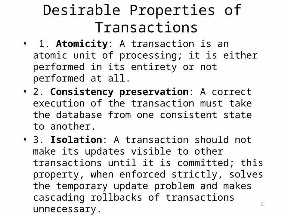
Desirable Properties of Transactions

• 1. Atomicity: A transaction is an atomic unit of processing; it is either performed in its entirety or not performed at all.

• 2. Consistency preservation: A correct execution of the transaction must take the database from one consistent state to another.

• 3. Isolation: A transaction should not make its updates visible to other transactions until it is committed; this property, when enforced strictly, solves the temporary update problem and makes cascading rollbacks of transactions unnecessary.

• 4. Durability or permanency: Once a transaction changes the database and the changes are committed, these changes must never be lost because of subsequent failure.

2

Why Concurrency Control?

• A Transaction: logical unit of database processing that includes one or more access operations (read retrieval, write insert or update, delete).

• Concurrency control is used to ensure the isolation property of concurrently executing transactions via protocols such as locking, timestamping, optimistic concurrency control…

3

Concurrency problems• 2 general problems can occur when there is

no proper concurrency control:– Lost update:– Temporary update (dirty read)

• Essentially they both break the isolation property of database transactions– Make updates visible to other transactions before

they are committed to the database– There is a conflict in the schedule

4

Example 1: Lost Updates

Transactions– User X: Updating Customer A account with withdrawal of $50– User Y: Updating Customer A account with deposit of $25– Customers balance should be (100 –50 + 25 = 75)

USER X USER Y

1 Read Cust A record (Balance = $100) 1 Read Cust A record

(Balance = $100)2 Bal = Bal - 50

(Balance = $50) 2 Bal = Bal + 25 (Balance = $125)

3 Write Cust A record (Balance = $50) 3 Write Cust A record

(Balance = $125)

5

Time

Example 3:Temporary Update ProblemTransactions

– A update to a product that that falters– A product update that completes

USER X USER Y

1 Read Prod A record(QOH = 35)

2 Update QOH (+100)3 Write Prod A record (QOH

= 135) 1 Read Prod A QOH (QOH = 135)2 Update QOH (-30) (QOH = 105)

4 Failure: Rollback3 Write Prod A QOH (QOH = 105)

Begin Recovery… 4 ….commit;

6

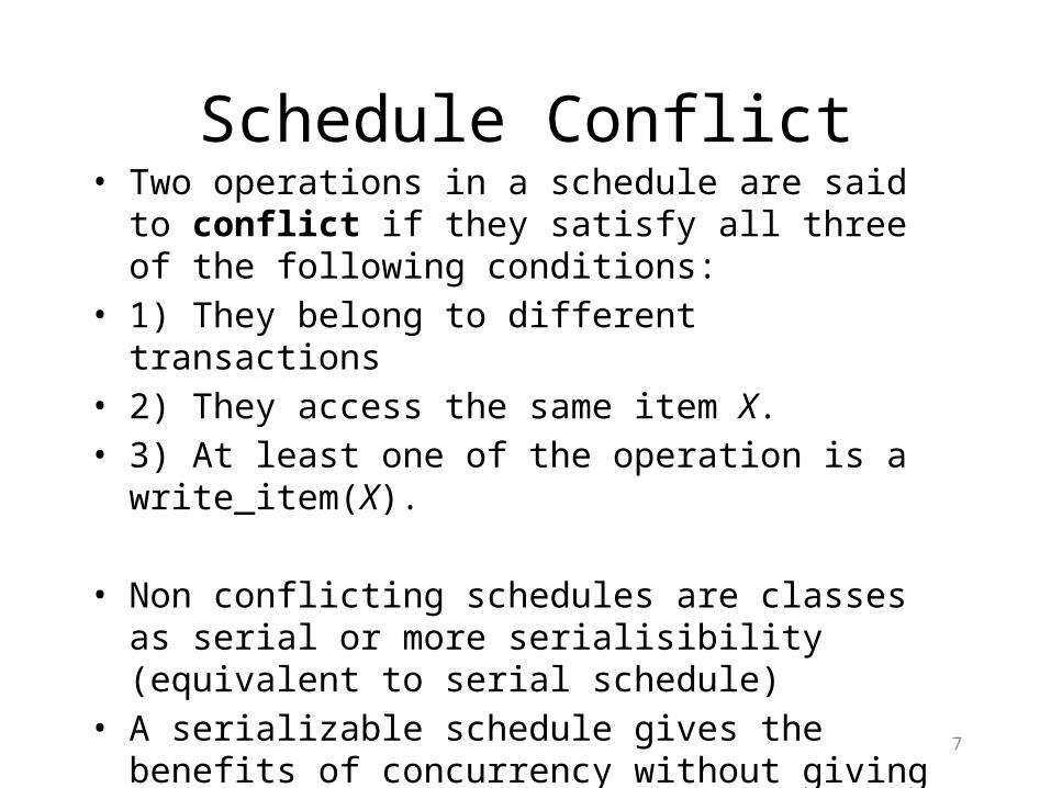
Schedule Conflict• Two operations in a schedule are said to conflict if they

satisfy all three of the following conditions:• 1) They belong to different transactions• 2) They access the same item X.• 3) At least one of the operation is a write_item(X).

• Non conflicting schedules are classes as serial or more serialisibility (equivalent to serial schedule)

• A serializable schedule gives the benefits of concurrency without giving up correctness.

7

8

CLASSIFICATION OF CONCURRENCY CONTROL TECHNIQUES

• 1. Locking data items to prevent multiple transactions from accessing the items concurrently; a number of locking protocols have been proposed.

• 2. Use of timestamps. A timestamp is a unique identifier • for each transaction, generated by the system. • 3. Optimistic Concurrency Control: based on the concept of validation or

certification of a transaction after it executes its operations; these are sometimes called optimistic protocols. They proceed optimistically; back up and repair if needed

• 4. Pessimistic protocol: do not proceed until knowing that no back up is needed.

9

Two-Phase Locking

• transaction divided into 2 phases:• – growing - new locks acquired but

none released• – shrinking - existing locks released

but no new ones acquired

10

Two-Phase Locking (cont.)

• If every transaction in a schedule follows the two phase locking protocol, the schedule is guaranteed to be serializable i.e. no concurrency problems will occur.

• The two phase locking protocol guarantees serializability however the use of locks can cause two additional problems: deadlock and starvation.

11

12

DEADLOCK PREVENTION:

• Use of transaction timestamp TS(T)• Two protocols can be used to prevent or more

precisely roll-back one transaction in the case of deadlock.– Wait-die (older transaction waits for a younger

one…)– Wound –wait protocol (younger waits for older

transaction to finish)

13

Timestamping protocol

Transaction Timestamps: the time the transaction starts

Data Timestamps• Read-Timestamp is timestamp of largest timestamp to read that

data item• Write-Timestamp is timestamp of largest timestamp to write

(update) that data item

• Timestamping prevents deadlock and starvation

Concurrency control using Timestamp• Basic timestamp methods

– Write- operation• When a Transaction attempts a write operation on a

data item X it must first check that X has not been read or updated by a younger transaction: proceeds if no and rolled back if yes.

– Read operation• When a Transaction attempts a read operation on a

data item X it must first check that X has not been updated by a younger transaction.proceeds if no and rolled back if yes.

15

Concurrency Control based on Timestamps

• The basic idea or rules are as follows:– 1. Each transaction receives a timestamp when it is initiated at its site of

origin.– 2. Each read or write operation which is required by a transaction has the

timestamp of the transaction.– 3. For each data item x, the largest timestamp of a read operation and the

largest timestamp of a write operation are recorded; they will be indicated as TRD(x) and TWR(x)

– 4. Let T be the timestamp of a read operation on data item x. If T < TWR(x), the read operation is rejected and the issuing transaction restarted with a new timestamp; otherwise, the read is executed, and TRD(x) = max(TRD(x), T).

– 5. Let T be the timestamp of a write operation on data item x. If T < TWR(x) or T < TRD(x), then the operation is rejected and the issuing transaction is restarted; otherwise, the write is executed, and TWR(x) = T.

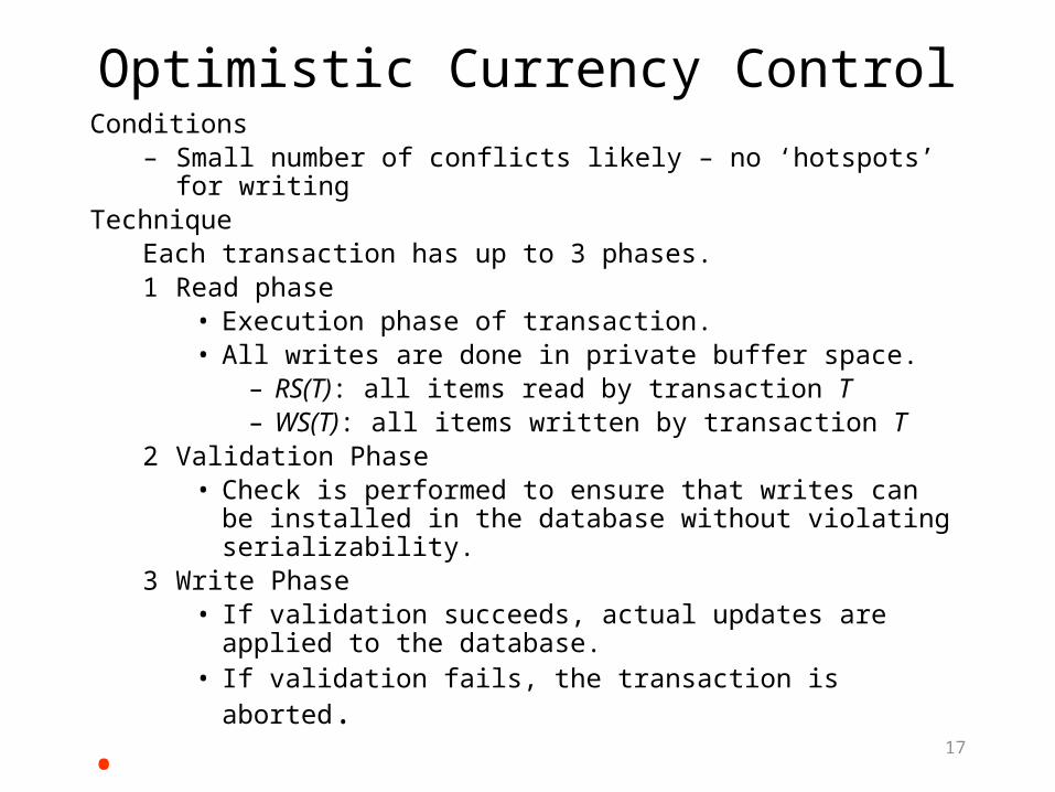
Optimistic Currency ControlConditions

– Small number of conflicts likely – no ‘hotspots’ for writing Technique

Each transaction has up to 3 phases.1 Read phase

• Execution phase of transaction.• All writes are done in private buffer space.

– RS(T): all items read by transaction T– WS(T): all items written by transaction T

2 Validation Phase• Check is performed to ensure that writes can be installed in the

database without violating serializability.3 Write Phase

• If validation succeeds, actual updates are applied to the database.• If validation fails, the transaction is aborted.

•

17

Question to consider

• Explain / illustrate each of the concurrency control methods prevents the violation of the ACID properities.

18

19

Review Recovery

Denis ManleyEnterprise Systems

DT211 4

RECOVERY TECHNIQUES ARE NEEDED BECAUSE

TRANSACTIONS MAY FAIL 1. A computer failure or system crash: A hard ware or software error occurs

during transaction execution. 2. Concurrency control enforcement: The concurrency control method may

decide to abort the transaction3. Disk failure: Some disk blocks may lose their data because of a read or

write malfunction or because of a disk read/write head crash. 4. Physical problems and catastrophes: This refers to an endless list of

problems that includes power or air conditioning failure, fire. Need disaster recovery as well for such problems .

•

20

The System Log• T is the system generated transaction-id.• 1. [start_transaction,T]: Records that transaction T has

started execution. • 2. [write_item,T,X,old_value,new_value]: Records that

transaction T has changed the value of database item X from old_value to new_value.

• 3. [read_item,T,X]: Records that transaction T has read the value of database item X

• 4. [commit,T]: Records that transaction T has completed successfully, and affirms that its effect can be committed to the DB.

• 5. [abort,T]: Records that transaction T has aborted.21

RECOVERY USING LOG RECORDS

• If the system crashes, we can recover to a consistent database state by examining the log. – It is possible to undo the effect of these WRITE operations

of a transaction T by tracing backward through the log and resetting all items changed by a WRITE operation of T to their old_values.

– We can also redo the effect of the WRITE operations of a transaction T by tracing forward through the log and setting all items changed by a WRITE operation of T to their new values.

22

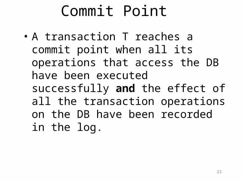
Commit Point

• A transaction T reaches a commit point when all its operations that access the DB have been executed successfully and the effect of all the transaction operations on the DB have been recorded in the log.

23

Undo/redo• UNDO/REDO (Immediate update):

– write-ahead to log on disk– update database anytime– commit allowed before database is completely updated

• Goal: Maximize efficiency during normal operation.– Some extra work is required during recovery time.

• Following a failure, the following is done.– Redo all transactions for which the log has both “start” and

“commit” entries.– Undo all transactions for which the log has “start” entry but

no “commit” entry.

24

Example of undo/redo• We consider two transactions executed sequentially by

the system.

• T1: Read(A) T2: Read(A)A A + 50 A A +10Read(B) Write(A)B B + 100 Read(D)Write(B) D D -10Read(C) Read(E)C 2C Read(B)Write(C) E E + BA A + B + C Write(E)Write (A) D D + EWrite(D)

• The initial values are:A=100 B=300 C=5 D=60 E=80

25

Example (cont)• The Log

1. <T1 starts>2. <T1, B, old: 300, new: 400>3. <T1, C, old: 5, new: 10>4. <T1, A, old: 100, new: 560>5. <T1 commits>6. <T2 starts>7. <T2, A, old: 560, new: 570>8. <T2, E, old: 80, new: 480>9. <T2, D, old: 60, new: 530>10. <T2 commits>

• Output of B can occur anytime after entry 2 is output to the log, etc. Determine action at T = 1, 1 =< T =< 4, 5= < T=< 9, T =10

26

Example (cont)• Assume a system crash occurs. The log is examined.

Various actions are taken depending on the last instruction (actually) written on it.

27

Last Instruction Action Consequence

I = 0 Nothing Neither T1 nor T2 has run

1 I 4 Undo T1: Restore the values of variables listed in 1-I old values

T1 has not run

5 I 9 Redo T1: Set the values of the variables listed in I-4 to values created by T1 Undo T2: Restore the values of variables listed in I-9 to those before T2 started execution

T1 ran T2 has not run

I=10 Redo T1 Redo T2

T1 and T2 both ran

No-Undo/Redo• NO-UNDO/REDO (Deferred update):

– don’t change database until ready to commit– write-ahead to log to disk– change the database after commit is recorded in the log

• Advantages– Faster during recovery: no undo.– No before images needed in log.

• Disadvantages– Database outputs must wait.– Lots of extra work at commit time.

28

Undo/No-Redo• UNDO/NO-REDO (Immediate update):

– All changed data items need to be output to the disk before commit.• Requires that the write entry first be output to the (stable) log.

– At commit:• Output (flush) all changed data items in the cache.• Add commit entry to log.

• Advantages– No after images are needed in log.– No transactions need to be redone.

• Disadvantages– data requires a flush for each committed write.

• Implies lots of I/O traffic.

29

No-Undo/No-Redo• NO-UNDO/NO-REDO (shadow paging):

– No-undo don't change the database during a transaction– No-redo on commit, write changes to the database in a single

atomic action

• Advantages– Recovery is instantaneous.– No recovery code need be written.

30

Shadow paging • During a transaction:

• After preparing new directory for commit:

• After committing:

31

x y z

x y z

Last committed value of xLast committed value of yLast committed value of z

New version of xNew version of y

Master

x y z

x y z



Master

x y z

x y z



Master

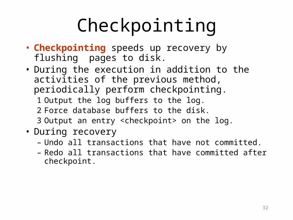
Checkpointing• Checkpointing speeds up recovery by flushing pages

to disk.• During the execution in addition to the activities of

the previous method, periodically perform checkpointing.1 Output the log buffers to the log.2 Force database buffers to the disk.3 Output an entry <checkpoint> on the log.

• During recovery– Undo all transactions that have not committed.– Redo all transactions that have committed after checkpoint.

32

Recovery with Checkpoints

• If the protocol is undo/redo then: – T1 is ok.– T2 and T3 are redone.– T4 is undone

33

Time

T1

T2

T3

T4

Tc Tf

System FailureCheckpoint

Question to consider

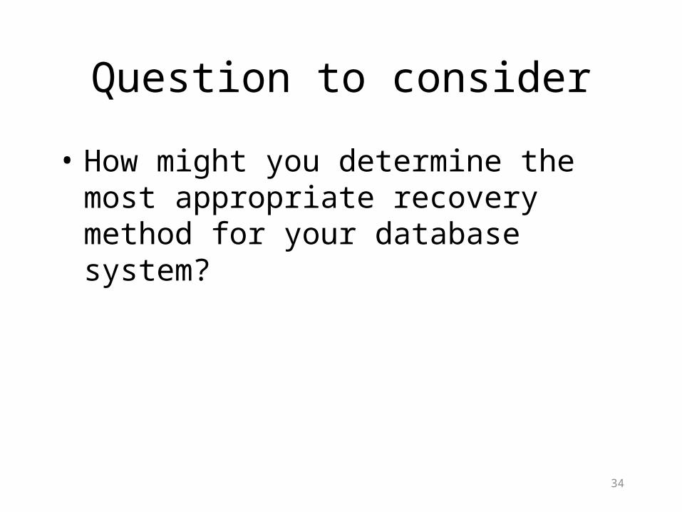
• How might you determine the most appropriate recovery method for your database system?

34

Review Query Optimisation

Denis ManleyEnterprise Systems

DT211 4

36

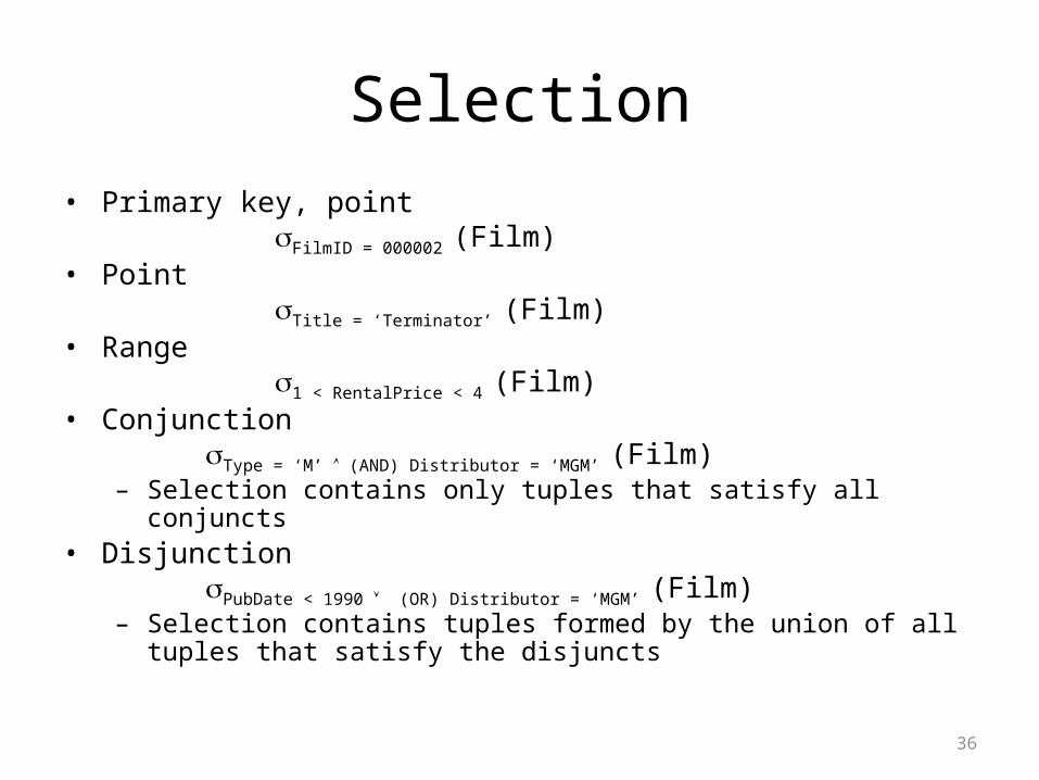
Selection• Primary key, point

sFilmID = 000002 (Film)• Point

sTitle = ‘Terminator’ (Film)• Range

s1 < RentalPrice < 4 (Film)• Conjunction

sType = ‘M’ (AND) Distributor = ‘MGM’ (Film)– Selection contains only tuples that satisfy all conjuncts

• DisjunctionsPubDate < 1990 (OR) Distributor = ‘MGM’ (Film)

– Selection contains tuples formed by the union of all tuples that satisfy the disjuncts

37

Query Optimization• Transform query into faster, equivalent query

query

• Heuristic (logical) optimization Query tree (relational algebra) optimization Query graph optimization

• Cost-based (physical) optimization

equivalent query 1

equivalent query 2

equivalent query n

...

fasterquery

38

Steps in typical Heuristics Optimisation

Step 1: Decompose s operations.Step 2: Move s as far down the query tree as possible.Step 3: Rearrange leaf nodes to apply the most

restrictive s operations first.Step 4: Form joins from and subsequent s operations.Step 5: Decompose p and move down the query tree

as far as possible.Step 6: Identify candidates for combined operations.

39

Query Tree Optimization Example• What are the names of customers living on Elm

Street who have checked out “Terminator”?• SQL query:

SELECT NameFROM Customer CU, CheckedOut CH, Film FWHERE T.Title = ’Terminator’ AND F.FilmId = CH.FilmIDAND CU.CustomerID = CH.CustomerID and CU.Street = ‘Elm’

40

Canonical Query Tree

CU CH

F

pName

sTitle = ‘Terminator’ F.FilmId = CH.FilmID CU.CustomerID = CH.CustomerID CU.Street = ‘Elm’

41

Apply Selections Early

CU

CH

F

pName

sStreet = ‘Elm’

sCU.CustomerID = CH.CustomerID sTitle = ‘Terminator’

s F.FilmId = CH.FilmID

42

Apply More Restrictive Selections Early

F

CH

CU

pName

sTitle = ‘Terminator’

s F.FilmId = CH.FilmID sStreet = ‘Elm’

s CU.CustomerID = CH.CustomerID

43

Form Joins

F

CH CU

⋈ F.FilmId = CH.FilmID

⋈ CU.CustomerID = CH.CustomerID


sStreet = ‘Elm’

pName

44

Apply Projections Early

F

CHCU

pName



sStreet = ‘Elm’


pFilmID pFilmID, CustomerID

pFilmID, CustomerID

45

Example: Identify Combined Operations

F

CHCU

pName


n F.FilmId = CH.FilmID

sStreet = ‘Elm’

n CU.CustomerID = CH.CustomerID


pFilmID, CustomerID

1

2 3

4

46

Cost-Based Optimization• Use transformations to generate multiple candidate query trees

from the canonical query tree.• Measuring Cost

– Typically disk access is the predominant cost, and is also relatively easy to estimate.

– Therefore number of block transfers from disk is used as a measure of the actual cost of evaluation.

– It is assumed that all transfers of blocks have the same cost.• Do not include cost to writing output to disk.• Cost formulas estimate the cost of executing each operation in each

candidate query tree.• The candidate query tree with the least total cost is selected for

execution.

47

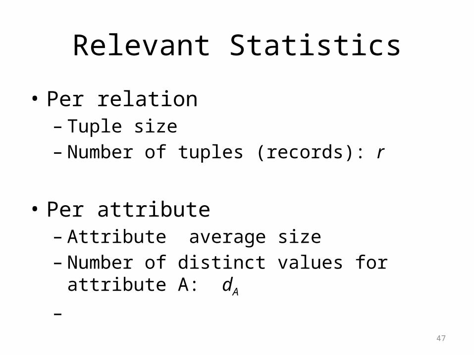
Relevant Statistics

• Per relation– Tuple size– Number of tuples (records): r

• Per attribute– Attribute average size – Number of distinct values for attribute A: dA –

48

Cost Estimation Example

F

CHCU

pName



sStreet = ‘Elm’



pFilmID, CustomerID

1

2 3

4

49

Operation 1: s followed by a p• Statistics

– Relation statistics: rFilm= 5,000

– Attribute statistics: sTitle= 1

• Result relation size: 1 tuple.• Cost (in disk accesses): C1 = 1

• Statistics– Relation statistics: rCheckedOut= 40,000

– Attribute statistics: sFilmID= 8

• Result relation size: 8 tuples.• Cost: C2 = 8

50

Operation 3: s followed by a p

• Statistics– Relation statistics: rCustomer= 200

– Attribute statistics:sStreet= 10

• Result relation size: 10 tuples.• Cost: C3 = 10

• Operation: Main memory join on relations in main memory.• Cost: C4 = 0

Total cost: 19

51

Operation 4: followed by a ⋈ p

• Operation: Main memory join on relations in main memory.

• Cost: C4 = 0

Total cost:

19010814

1

i

iCC

52

Summary

• Query optimization is the heart of a relational DBMS.

• Heuristic optimization is more efficient to generate, but may not yield the optimal query evaluation plan.

• Cost-based optimization relies on statistics gathered on the relations.

• Note: Query optimisation is more critical for larger distributed database systems

Documents

Review Concurrency Enterprise Systems architecture and infrastructure DT211 4 1