Final Exam Review

2

Chapter 6 Dynamic Programming

Slides by Kevin Wayne. Copyright © 2005 Pearson-Addison Wesley. All rights reserved.

12

Knapsack Problem

Knapsack problem. ■  Given n objects and a "knapsack." ■  Item i weighs wi > 0 kilograms and has value vi > 0. ■  Knapsack has capacity of W kilograms. ■  Goal: fill knapsack so as to maximize total value.

Ex: { 3, 4 } has value 40. Greedy: repeatedly add item with maximum ratio vi / wi. Ex: { 5, 2, 1 } achieves only value = 35 ⇒ greedy not optimal.

1

Value

18

22

28

1

Weight

5

6

6 2

7

Item

1

3

4

5

2 W = 11

13

Dynamic Programming: Adding a New Variable

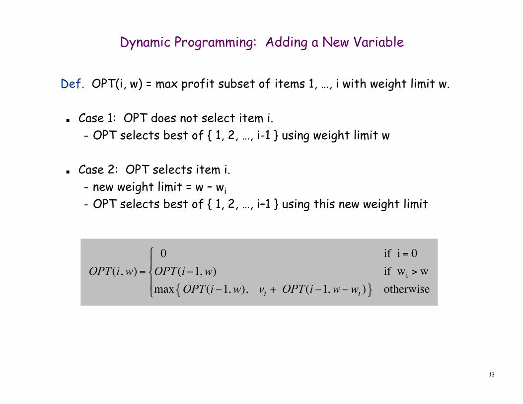
Def. OPT(i, w) = max profit subset of items 1, …, i with weight limit w.

■  Case 1: OPT does not select item i. –  OPT selects best of { 1, 2, …, i-1 } using weight limit w

■  Case 2: OPT selects item i. –  new weight limit = w – wi –  OPT selects best of { 1, 2, …, i–1 } using this new weight limit

€

OPT(i, w) =

0 if i = 0OPT(i −1, w) if wi > wmax OPT(i −1, w), vi + OPT(i −1, w−wi ){ } otherwise

#

$ %

& %

14

Knapsack Algorithm

n + 1

1

Value

18

22

28

1 Weight

5

6

6 2

7

Item 1

3

4

5

2

φ

{ 1, 2 }

{ 1, 2, 3 }

{ 1, 2, 3, 4 }

{ 1 }

{ 1, 2, 3, 4, 5 }

0

0

0

0

0

0

0

1

0

1

1

1

1

1

2

0

6

6

6

1

6

3

0

7

7

7

1

7

4

0

7

7

7

1

7

5

0

7

18

18

1

18

6

0

7

19

22

1

22

7

0

7

24

24

1

28

8

0

7

25

28

1

29

9

0

7

25

29

1

34

10

0

7

25

29

1

34

11

0

7

25

40

1

40

W + 1

W = 11 OPT: { 4, 3 } value = 22 + 18 = 40

17

Dynamic Programming Over Intervals

Notation. OPT(i, j) = maximum number of base pairs in a secondary structure of the substring bibi+1…bj.

■  Case 1. If i ≥ j - 4. –  OPT(i, j) = 0 by no-sharp turns condition.

■  Case 2. Base bj is not involved in a pair. –  OPT(i, j) = OPT(i, j-1)

■  Case 3. Base bj pairs with bt for some i ≤ t < j - 4. –  non-crossing constraint decouples resulting sub-problems –  OPT(i, j) = 1 + maxt { OPT(i, t-1) + OPT(t+1, j-1) }

Remark. Same core idea in CKY algorithm to parse context-free grammars.

take max over t such that i ≤ t < j-4 and bt and bj are Watson-Crick complements

18

Dynamic Programming Summary

Recipe. ■  Characterize structure of problem. ■  Recursively define value of optimal solution. ■  Compute value of optimal solution. ■  Construct optimal solution from computed information.

Dynamic programming techniques. ■  Binary choice: weighted interval scheduling. ■  Multi-way choice: segmented least squares. ■  Adding a new variable: knapsack. ■  Dynamic programming over intervals: RNA secondary structure.

Top-down vs. bottom-up: different people have different intuitions.

Viterbi algorithm for HMM also uses DP to optimize a maximum likelihood tradeoff between parsimony and accuracy

CKY parsing algorithm for context-free grammar has similar structure

20

String Similarity

How similar are two strings? ■  ocurrance

■  occurrence

o c u r r a n c e

c c u r r e n c e o

-

o c u r r n c e

c c u r r n c e o

- - a

e -

o c u r r a n c e

c c u r r e n c e o

-

5 mismatches, 1 gap

1 mismatch, 1 gap

0 mismatches, 3 gaps

21

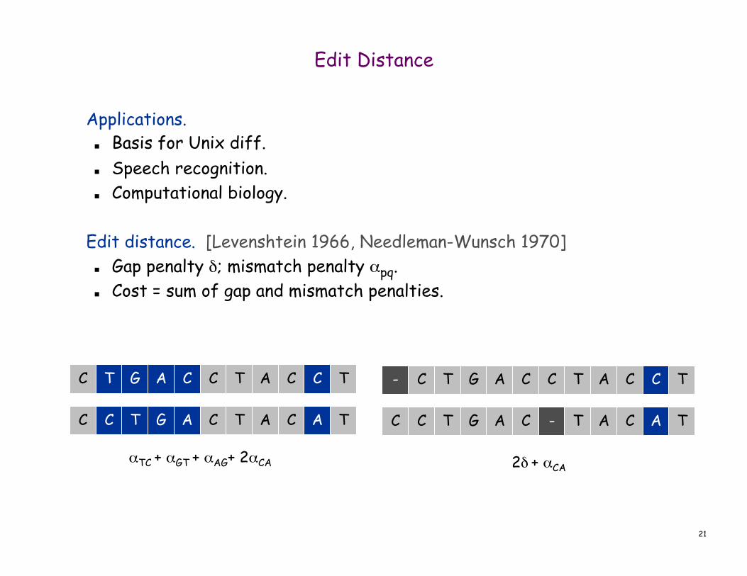
Applications. ■  Basis for Unix diff. ■  Speech recognition. ■  Computational biology.

Edit distance. [Levenshtein 1966, Needleman-Wunsch 1970]

■  Gap penalty δ; mismatch penalty αpq. ■  Cost = sum of gap and mismatch penalties.

2δ + αCA

C G A C C T A C C T

C T G A C T A C A T

T G A C C T A C C T

C T G A C T A C A T

- T

C

C

C

αTC + αGT + αAG+ 2αCA

-

Edit Distance

22

Goal: Given two strings X = x1 x2 . . . xm and Y = y1 y2 . . . yn find alignment of minimum cost. Def. An alignment M is a set of ordered pairs xi-yj such that each item occurs in at most one pair and no crossings.

Def. The pair xi-yj and xi'-yj' cross if i < i', but j > j'.

Ex: CTACCG vs. TACATG. Sol: M = x2-y1, x3-y2, x4-y3, x5-y4, x6-y6.

Sequence Alignment

€

cost( M ) = αxi y j(xi, y j )∈ M∑

mismatch

+ δi : xi unmatched

∑ + δj : y j unmatched

∑

gap

C T A C C -

T A C A T -

G

G y1 y2 y3 y4 y5 y6

x2 x3 x4 x5 x1 x6

23

Sequence Alignment: Problem Structure

Def. OPT(i, j) = min cost of aligning strings x1 x2 . . . xi and y1 y2 . . . yj. ■  Case 1: OPT matches xi-yj.

–  pay mismatch for xi-yj + min cost of aligning two strings x1 x2 . . . xi-1 and y1 y2 . . . yj-1

■  Case 2a: OPT leaves xi unmatched. –  pay gap for xi and min cost of aligning x1 x2 . . . xi-1 and y1 y2 . . . yj

■  Case 2b: OPT leaves yj unmatched. –  pay gap for yj and min cost of aligning x1 x2 . . . xi and y1 y2 . . . yj-1

€

OPT(i, j) =

"

#

$ $ $

%

$ $ $

jδ if i = 0

min

αxi y j+ OPT(i −1, j −1)

δ + OPT(i −1, j)δ + OPT(i, j −1)

"

# $

% $

otherwise

iδ if j = 0

24

Divide: find index q that minimizes f(q, n/2) + g(q, n/2) using DP. ■  Align xq and yn/2.

Conquer: recursively compute optimal alignment in each piece.

Sequence Alignment: Linear Space

i-j x1

x2

y1

x3

y2 y3 y4 y5 y6

ε

ε

0-0

q

n / 2

m-n

26

Shortest Paths

Shortest path problem. Given a directed graph G = (V, E), with edge weights cvw, find shortest path from node s to node t. Ex. Nodes represent agents in a financial setting and cvw is cost of transaction in which we buy from agent v and sell immediately to w.

s

3

t

2

6

7

4 5

10

18 -16

9

6

15 -8

30

20

44

16

11

6

19

6

allow negative weights

27

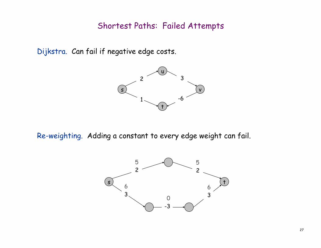
Shortest Paths: Failed Attempts

Dijkstra. Can fail if negative edge costs. Re-weighting. Adding a constant to every edge weight can fail.

u

t

s v

2

1

3

-6

s t

2

3

2

-3

3

5 5

6 6

0

28

Shortest Paths: Dynamic Programming

Def. OPT(i, v) = length of shortest v-t path P using at most i edges.

■  Case 1: P uses at most i-1 edges. –  OPT(i, v) = OPT(i-1, v)

■  Case 2: P uses exactly i edges. –  if (v, w) is first edge, then OPT uses (v, w), and then selects best

w-t path using at most i-1 edges

Remark. By previous observation, if no negative cycles, then OPT(n-1, v) = length of shortest v-t path.

€

OPT(i, v) = 0 if i = 0

min OPT(i −1, v) ,(v, w)∈ E

min OPT(i −1, w)+ cvw{ }$ % &

' ( )

otherwise

$

% *

& *

29

Shortest Paths: Implementation

Analysis. Θ(mn) time, Θ(n2) space. Finding the shortest paths. Maintain a "successor" for each table entry.

Shortest-Path(G, t) { foreach node v ∈ V M[0, v] ← ∞ M[0, t] ← 0 for i = 1 to n-1 foreach node v ∈ V M[i, v] ← M[i-1, v] foreach edge (v, w) ∈ E M[i, v] ← min { M[i, v], M[i-1, w] + cvw } }

30

Chapter 7 Network Flow

Slides by Kevin Wayne. Copyright © 2005 Pearson-Addison Wesley. All rights reserved.

31

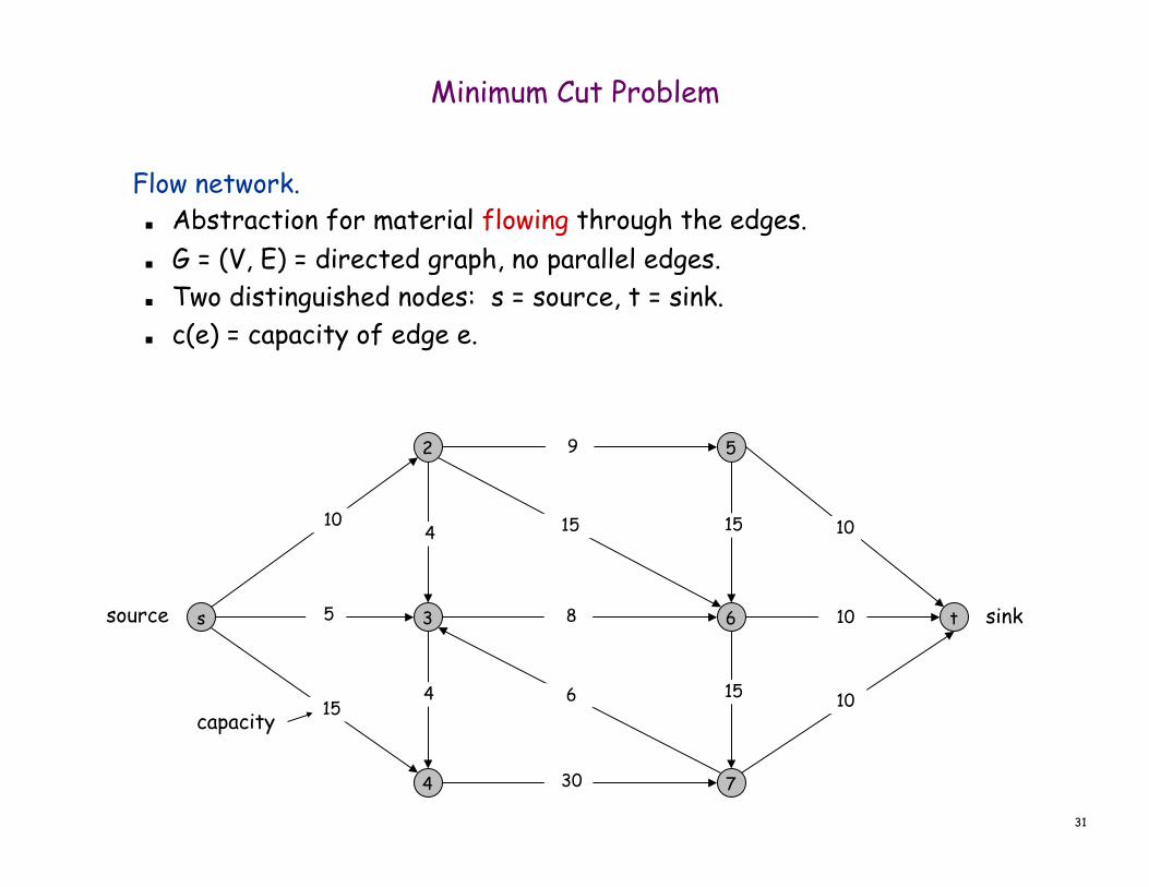
Flow network. ■  Abstraction for material flowing through the edges. ■  G = (V, E) = directed graph, no parallel edges. ■  Two distinguished nodes: s = source, t = sink. ■  c(e) = capacity of edge e.

Minimum Cut Problem

s

2

3

4

5

6

7

t

15

5

30

15

10

8

15

9

6 10

10

10 15 4

4 capacity

source sink

32

Flow value lemma. Let f be any flow, and let (A, B) be any s-t cut. Then, the net flow sent across the cut is equal to the amount leaving s.

Flows and Cuts

10

6

6

11

1 10

3 8 8

0 0

0

11

s

2

3

4

5

6

7

t

15

5

30

15

10

8

15

9

6 10

10

10 15 4

4 0

€

f (e)e out of A∑ − f (e)

e in to A∑ = v( f )

Value = 10 - 4 + 8 - 0 + 10 = 24

4

A

33

Weak duality. Let f be any flow. Then, for any s-t cut (A, B) we have v(f) ≤ cap(A, B). Pf.

▪

Flows and Cuts

€

v( f ) = f (e)e out of A∑ − f (e)

e in to A∑

≤ f (e)e out of A∑

≤ c(e)e out of A∑

= cap(A,B)s

t

A B

7

6

8 4

34

Certificate of Optimality

Corollary. Let f be any flow, and let (A, B) be any cut. If v(f) = cap(A, B), then f is a max flow and (A, B) is a min cut.

Value of flow = 28 Cut capacity = 28 ⇒ Flow value ≤ 28

10

9

9

14

4 10

4 8 9

1

0 0

0

14

s

2

3

4

5

6

7

t

15

5

30

15

10

8

15

9

6 10

10

10 15 4

4 0 A

35

Max-Flow Min-Cut Theorem

Augmenting path theorem. Flow f is a max flow iff there are no augmenting paths. Max-flow min-cut theorem. [Ford-Fulkerson 1956] The value of the max flow is equal to the value of the min cut. Proof strategy. We prove both simultaneously by showing the TFAE: (i) There exists a cut (A, B) such that v(f) = cap(A, B). (ii) Flow f is a max flow. (iii) There is no augmenting path relative to f.

(i) ⇒ (ii) This was the corollary to weak duality lemma. (ii) ⇒ (iii) We show contrapositive. ■  Let f be a flow. If there exists an augmenting path, then we can

improve f by sending flow along path.

36

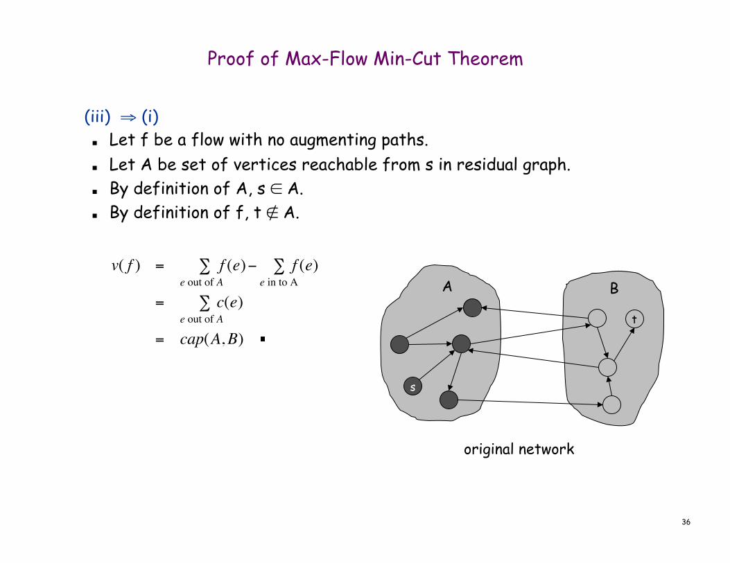
Proof of Max-Flow Min-Cut Theorem

(iii) ⇒ (i) ■  Let f be a flow with no augmenting paths. ■  Let A be set of vertices reachable from s in residual graph. ■  By definition of A, s ∈ A. ■  By definition of f, t ∉ A.

€

v( f ) = f (e)e out of A∑ − f (e)

e in to A∑

= c(e)e out of A∑

= cap(A,B)

original network

s

t

A B

37

Running Time

Assumption. All capacities are integers between 1 and C. Invariant. Every flow value f(e) and every residual capacities cf (e) remains an integer throughout the algorithm. Theorem. The algorithm terminates in at most v(f*) ≤ nC iterations. Pf. Each augmentation increase value by at least 1. ▪ Corollary. If C = 1, Ford-Fulkerson runs in O(m) time. Integrality theorem. If all capacities are integers, then there exists a max flow f for which every flow value f(e) is an integer. Pf. Since algorithm terminates, theorem follows from invariant. ▪

38

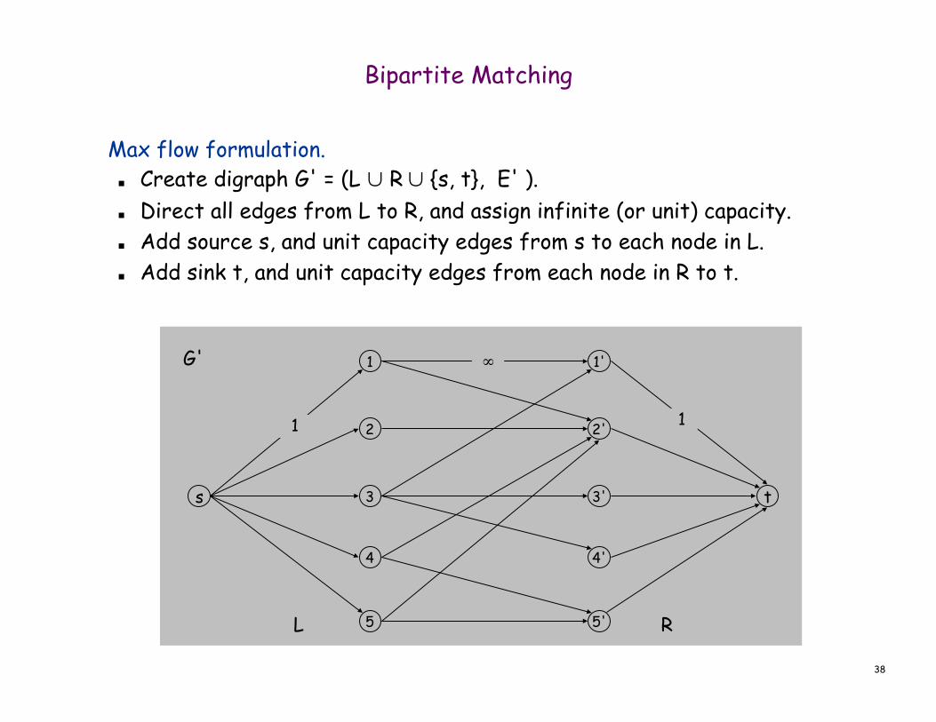
Max flow formulation. ■  Create digraph G' = (L ∪ R ∪ {s, t}, E' ). ■  Direct all edges from L to R, and assign infinite (or unit) capacity. ■  Add source s, and unit capacity edges from s to each node in L. ■  Add sink t, and unit capacity edges from each node in R to t.

Bipartite Matching

s

1

3

5

1'

3'

5'

t

2

4

2'

4'

1 1

∞

R L

G'

39

Disjoint path problem. Given a digraph G = (V, E) and two nodes s and t, find the max number of edge-disjoint s-t paths. Def. Two paths are edge-disjoint if they have no edge in common.

Ex: communication networks.

s

2

3

4

Edge Disjoint Paths

5

6

7

t

40

Network connectivity. Given a digraph G = (V, E) and two nodes s and t, find min number of edges whose removal disconnects t from s. Def. A set of edges F ⊆ E disconnects t from s if all s-t paths uses at least on edge in F.

Network Connectivity

s

2

3

4

5

6

7

t

41

Disjoint Paths and Network Connectivity

Theorem. [Menger 1927] The max number of edge-disjoint s-t paths is equal to the min number of edges whose removal disconnects t from s. Pf. ≥ ■  Suppose max number of edge-disjoint paths is k. ■  Then max flow value is k. ■  Max-flow min-cut ⇒ cut (A, B) of capacity k. ■  Let F be set of edges going from A to B. ■  |F| = k and disconnects t from s. ▪

s

2

3

4

5

6

7

t s

2

3

4

5

6

7

t

A

42

Chapter 8 NP and Computational Intractability

Slides by Kevin Wayne. Copyright © 2005 Pearson-Addison Wesley. All rights reserved.

43

Polynomial-Time Reduction

Purpose. Classify problems according to relative difficulty. Design algorithms. If X ≤ P Y and Y can be solved in polynomial-time, then X can also be solved in polynomial time. Establish intractability. If X ≤ P Y and X cannot be solved in polynomial-time, then Y cannot be solved in polynomial time. Establish equivalence. If X ≤ P Y and Y ≤ P X, we use notation X ≡ P Y.

up to cost of reduction

44

Vertex Cover and Independent Set

Claim. VERTEX-COVER ≡P INDEPENDENT-SET. Pf. We show S is an independent set iff V - S is a vertex cover.

vertex cover

independent set

45

Vertex Cover and Independent Set

Claim. VERTEX-COVER ≡P INDEPENDENT-SET. Pf. We show S is an independent set iff V - S is a vertex cover. ⇒ ■  Let S be any independent set. ■  Consider an arbitrary edge (u, v). ■  S independent ⇒ u ∉ S or v ∉ S ⇒ u ∈ V - S or v ∈ V - S. ■  Thus, V - S covers (u, v).

⇐ ■  Let V - S be any vertex cover. ■  Consider two nodes u ∈ S and v ∈ S. ■  Observe that (u, v) ∉ E since V - S is a vertex cover. ■  Thus, no two nodes in S are joined by an edge ⇒ S independent set. ▪

46

Set Cover

SET COVER: Given a set U of elements, a collection S1, S2, . . . , Sm of subsets of U, and an integer k, does there exist a collection of ≤ k of these sets whose union is equal to U?

Sample application. ■  m available pieces of software. ■  Set U of n capabilities that we would like our system to have. ■  The ith piece of software provides the set Si ⊆ U of capabilities. ■  Goal: achieve all n capabilities using fewest pieces of software.

Ex:

U = { 1, 2, 3, 4, 5, 6, 7 } k = 2 S1 = {3, 7} S4 = {2, 4} S2 = {3, 4, 5, 6} S5 = {5} S3 = {1} S6 = {1, 2, 6, 7}

47

SET COVER U = { 1, 2, 3, 4, 5, 6, 7 } k = 2 Sa = {3, 7} Sb = {2, 4} Sc = {3, 4, 5, 6} Sd = {5} Se = {1} Sf= {1, 2, 6, 7}

Vertex Cover Reduces to Set Cover

Claim. VERTEX-COVER ≤ P SET-COVER. Pf. Given a VERTEX-COVER instance G = (V, E), k, we construct a set cover instance whose size equals the size of the vertex cover instance. Construction. ■  Create SET-COVER instance:

–  k = k, U = E, Sv = {e ∈ E : e incident to v } ■  Set-cover of size ≤ k iff vertex cover of size ≤ k. ▪

a

d

b

e

f c

VERTEX COVER

k = 2 e1

e2 e3

e5

e4

e6

e7

48

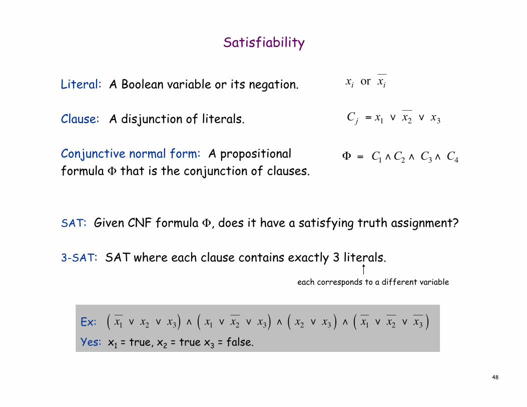
Ex:

Yes: x1 = true, x2 = true x3 = false.

Literal: A Boolean variable or its negation. Clause: A disjunction of literals. Conjunctive normal form: A propositional formula Φ that is the conjunction of clauses. SAT: Given CNF formula Φ, does it have a satisfying truth assignment? 3-SAT: SAT where each clause contains exactly 3 literals.

Satisfiability

€

Cj = x1 ∨ x2 ∨ x3

€

xi or xi

€

Φ = C1 ∧C2 ∧ C3∧ C4

€

x1 ∨ x2 ∨ x3( ) ∧ x1 ∨ x2 ∨ x3( ) ∧ x2 ∨ x3( ) ∧ x1 ∨ x2 ∨ x3( )

each corresponds to a different variable

49

3 Satisfiability Reduces to Independent Set

Claim. 3-SAT ≤ P INDEPENDENT-SET. Pf. Given an instance Φ of 3-SAT, we construct an instance (G, k) of INDEPENDENT-SET that has an independent set of size k iff Φ is satisfiable. Construction. ■  G contains 3 vertices for each clause, one for each literal. ■  Connect 3 literals in a clause in a triangle. ■  Connect literal to each of its negations.

€

x2

€

Φ = x1 ∨ x2 ∨ x3( ) ∧ x1 ∨ x2 ∨ x3( ) ∧ x1 ∨ x2 ∨ x4( )

€

x3

€

x1

€

x1

€

x2

€

x4

€

x1

€

x2

€

x3

k = 3

G

51

Review

Basic reduction strategies. ■  Simple equivalence: INDEPENDENT-SET ≡ P VERTEX-COVER. ■  Special case to general case: VERTEX-COVER ≤ P SET-COVER. ■  Encoding with gadgets: 3-SAT ≤ P INDEPENDENT-SET.

Transitivity. If X ≤ P Y and Y ≤ P Z, then X ≤ P Z. Pf idea. Compose the two algorithms. Ex: 3-SAT ≤ P INDEPENDENT-SET ≤ P VERTEX-COVER ≤ P SET-COVER.

52

Decision Problems

Decision problem. ■  X is a set of strings. ■  Instance: string s. ■  Algorithm A solves problem X: A(s) = yes iff s ∈ X.

Polynomial time. Algorithm A runs in poly-time if for every string s, A(s) terminates in at most p(|s|) "steps", where p(⋅) is some polynomial.

Def. Algorithm C(s, t) is a certifier for problem X if for every string s, s ∈ X iff there exists a string t such that C(s, t) = yes.

NP. Decision problems for which there exists a poly-time certifier.

length of s

53

Certifiers and Certificates: 3-Satisfiability

SAT. Given a CNF formula Φ, is there a satisfying assignment? Certificate. An assignment of truth values to the n boolean variables. Certifier. Check that each clause in Φ has at least one true literal. Ex. Conclusion. SAT is in NP.

€

x1 ∨ x2 ∨ x3( ) ∧ x1 ∨ x2 ∨ x3( ) ∧ x1 ∨ x2 ∨ x4( ) ∧ x1 ∨ x3 ∨ x4( )

€

x1 =1, x2 =1, x3 = 0, x4 =1

instance s

certificate t

54

P, NP, EXP

P. Decision problems for which there is a poly-time algorithm. EXP. Decision problems for which there is an exponential-time algorithm. NP. Decision problems for which there is a poly-time certifier.

Claim. P ⊆ NP. Pf. Consider any problem X in P. ■  By definition, there exists a poly-time algorithm A(s) that solves X. ■  Certificate: t = ε, certifier C(s, t) = A(s). ▪

Claim. NP ⊆ EXP. Pf. Consider any problem X in NP. ■  By definition, there exists a poly-time certifier C(s, t) for X. ■  To solve input s, run C(s, t) on all strings t with |t| ≤ p(|s|). ■  Return yes, if C(s, t) returns yes for any of these. ▪

55

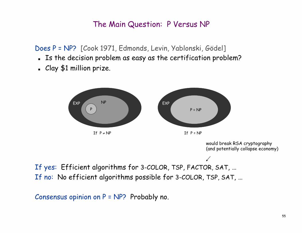
The Main Question: P Versus NP

Does P = NP? [Cook 1971, Edmonds, Levin, Yablonski, Gödel] ■  Is the decision problem as easy as the certification problem? ■  Clay $1 million prize.

If yes: Efficient algorithms for 3-COLOR, TSP, FACTOR, SAT, … If no: No efficient algorithms possible for 3-COLOR, TSP, SAT, …

Consensus opinion on P = NP? Probably no.

EXP NP

P

If P ≠ NP If P = NP

EXP P = NP

would break RSA cryptography (and potentially collapse economy)

56

NP-Complete

NP-complete. A problem Y in NP with the property that for every problem X in NP, X ≤ p Y.

Theorem. Suppose Y is an NP-complete problem. Then Y is solvable in poly-time iff P = NP. Pf. ⇐ If P = NP then Y can be solved in poly-time since Y is in NP. Pf. ⇒ Suppose Y can be solved in poly-time. ■  Let X be any problem in NP. Since X ≤ p Y, we can solve X in

poly-time. This implies NP ⊆ P. ■  We already know P ⊆ NP. Thus P = NP. ▪

Fundamental question. Do there exist "natural" NP-complete problems?

57

∧

¬

∧ ∨

∧

∨

1 0 ? ? ?

output

inputs hard-coded inputs

yes: 1 0 1

Circuit Satisfiability

CIRCUIT-SAT. Given a combinational circuit built out of AND, OR, and NOT gates, is there a way to set the circuit inputs so that the output is 1?

58

∧ ¬

u-v

∨

1

independent set of size 2?

n inputs (nodes in independent set) hard-coded inputs (graph description)

∨

∨

∧

u-w

0

∧

v-w

1

∧

u ?

∧

v ?

∧

w ?

∧

∨

set of size 2?

both endpoints of some edge have been chosen?

independent set?

Example

Ex. Construction below creates a circuit K whose inputs can be set so that K outputs true iff graph G has an independent set of size 2.

u

v w

€

n2

"

# $

%

& '

G = (V, E), n = 3

59

Establishing NP-Completeness

Remark. Once we establish first "natural" NP-complete problem, others fall like dominoes. Recipe to establish NP-completeness of problem Y. ■  Step 1. Show that Y is in NP. ■  Step 2. Choose an NP-complete problem X. ■  Step 3. Prove that X ≤ p Y.

Justification. If X is an NP-complete problem, and Y is a problem in NP with the property that X ≤ P Y then Y is NP-complete. Pf. Let W be any problem in NP. Then W ≤ P X ≤ P Y. ■  By transitivity, W ≤ P Y. ■  Hence Y is NP-complete. ▪ by assumption by definition of

NP-complete

60

3-SAT is NP-Complete

Theorem. 3-SAT is NP-complete. Pf. Suffices to show that CIRCUIT-SAT ≤ P 3-SAT since 3-SAT is in NP. ■  Let K be any circuit. ■  Create a 3-SAT variable xi for each circuit element i. ■  Make circuit compute correct values at each node:

–  x2 = ¬ x3 ⇒ add 2 clauses: –  x1 = x4 ∨ x5 ⇒ add 3 clauses: –  x0 = x1 ∧ x2 ⇒ add 3 clauses:

■  Hard-coded input values and output value.

–  x5 = 0 ⇒ add 1 clause: –  x0 = 1 ⇒ add 1 clause:

■  Final step: turn clauses of length < 3 into

clauses of length exactly 3. ▪ ∨

∧

¬

0 ? ?

output

x0

x2 x1

€

x2 ∨ x3 , x2 ∨ x3

€

x1 ∨ x4 , x1 ∨ x5 , x1 ∨ x4 ∨ x5

€

x0 ∨ x1 , x0 ∨ x2 , x0 ∨ x1 ∨ x2

x3 x4 x5

€

x5

€

x0

61

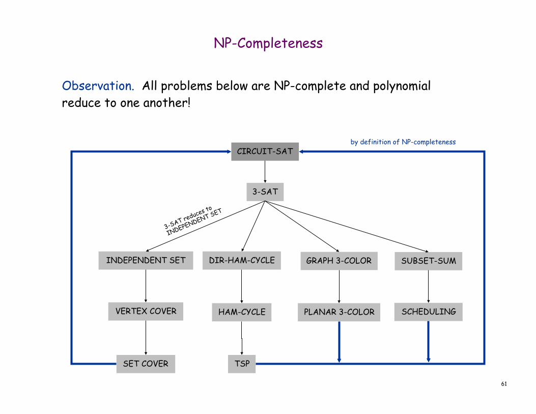
Observation. All problems below are NP-complete and polynomial reduce to one another!

CIRCUIT-SAT

3-SAT

DIR-HAM-CYCLE INDEPENDENT SET

VERTEX COVER

GRAPH 3-COLOR

HAM-CYCLE

TSP

SUBSET-SUM

SCHEDULING PLANAR 3-COLOR

SET COVER

NP-Completeness

by definition of NP-completeness

62

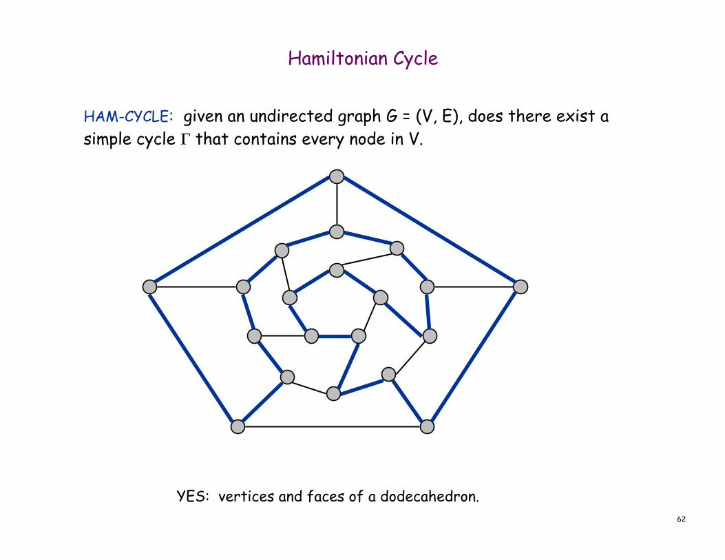
Hamiltonian Cycle

HAM-CYCLE: given an undirected graph G = (V, E), does there exist a simple cycle Γ that contains every node in V.

YES: vertices and faces of a dodecahedron.

63

Hamiltonian Cycle

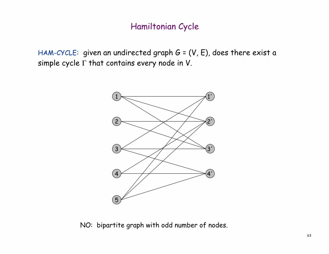
HAM-CYCLE: given an undirected graph G = (V, E), does there exist a simple cycle Γ that contains every node in V.

1

3

5

1'

3'

2

4

2'

4'

NO: bipartite graph with odd number of nodes.

65

Traveling Salesperson Problem

TSP. Given a set of n cities and a pairwise distance function d(u, v), is there a tour of length ≤ D? HAM-CYCLE: given a graph G = (V, E), does there exists a simple cycle that contains every node in V? Claim. HAM-CYCLE ≤ P TSP. Pf. ■  Given instance G = (V, E) of HAM-CYCLE, create n cities with distance

function

■  TSP instance has tour of length ≤ n iff G is Hamiltonian. ▪

Remark. TSP instance in reduction satisfies Δ-inequality.

€

d(u, v) = 1 if (u, v) ∈ E 2 if (u, v) ∉ E$ % &

66

Coping With NP-Completeness

Q. Suppose I need to solve an NP-complete problem. What should I do? A. Theory says you're unlikely to find poly-time algorithm.

Must sacrifice one of three desired features. ■  Solve problem to optimality. ■  Solve problem in polynomial time. ■  Solve arbitrary instances of the problem.

This lecture. Solve some special cases of NP-complete problems that arise in practice.

68

Vertex Cover

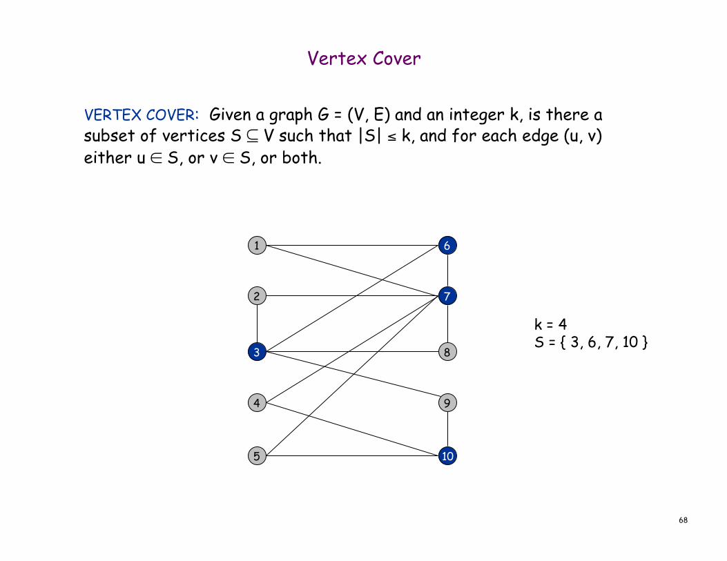
VERTEX COVER: Given a graph G = (V, E) and an integer k, is there a subset of vertices S ⊆ V such that |S| ≤ k, and for each edge (u, v) either u ∈ S, or v ∈ S, or both.

3

6

10

7

1

5

8

2

4 9

k = 4 S = { 3, 6, 7, 10 }

69

Finding Small Vertex Covers

Q. What if k is small? Brute force. O(k nk+1). ■  Try all C(n, k) = O(nk) subsets of size k. ■  Takes O(k n) time to check whether a subset is a vertex cover.

Goal. Limit exponential dependency on k, e.g., to O(2k k n). Ex. n = 1,000, k = 10. Brute. k nk+1 = 1034 ⇒ infeasible. Better. 2k k n = 107 ⇒ feasible. Remark. If k is a constant, algorithm is poly-time; if k is a small constant, then it's also practical.

71

Finding Small Vertex Covers: Algorithm

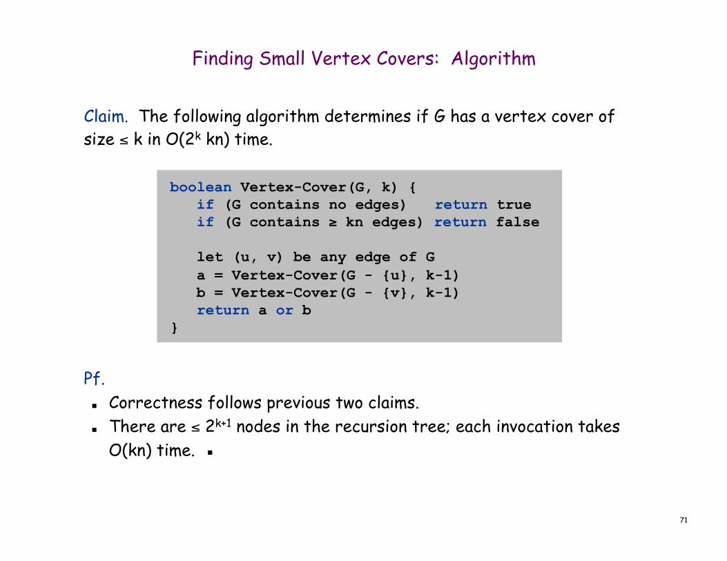
Claim. The following algorithm determines if G has a vertex cover of size ≤ k in O(2k kn) time. Pf. ■  Correctness follows previous two claims. ■  There are ≤ 2k+1 nodes in the recursion tree; each invocation takes

O(kn) time. ▪

boolean Vertex-Cover(G, k) { if (G contains no edges) return true if (G contains ≥ kn edges) return false let (u, v) be any edge of G a = Vertex-Cover(G - {u}, k-1) b = Vertex-Cover(G - {v}, k-1) return a or b }

72

Finding Small Vertex Covers: Recursion Tree

k

k-1 k-1

k-2 k-2 k-2 k-2

0 0 0 0 0 0 0 0

k - i

nkcknTkcknknTkcn

knT k2),( 1if)1,(2 1if

),( ≤⇒#$%

>+−

=≤

75

Independent Set on Trees: Greedy Algorithm

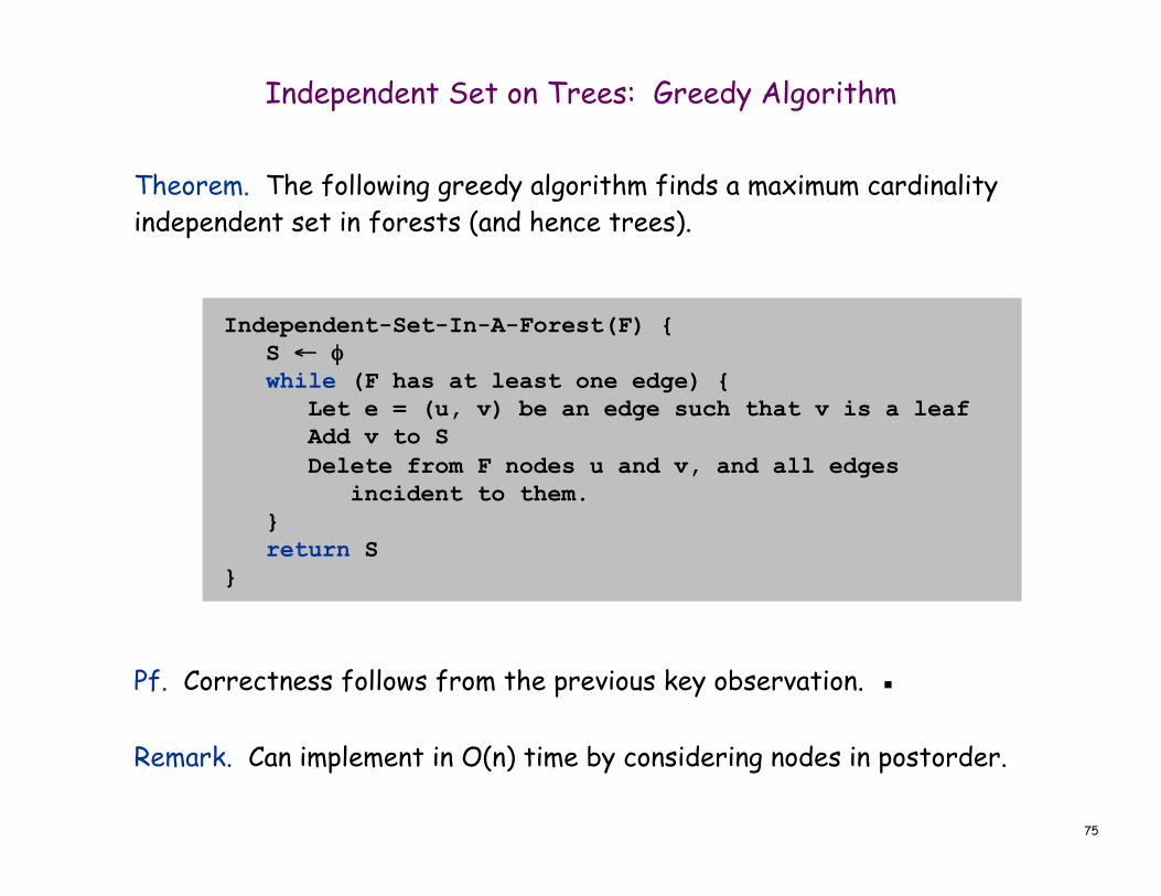
Theorem. The following greedy algorithm finds a maximum cardinality independent set in forests (and hence trees). Pf. Correctness follows from the previous key observation. ▪ Remark. Can implement in O(n) time by considering nodes in postorder.

Independent-Set-In-A-Forest(F) { S ← φ while (F has at least one edge) { Let e = (u, v) be an edge such that v is a leaf Add v to S Delete from F nodes u and v, and all edges incident to them. } return S }

76

Weighted Independent Set on Trees

Weighted independent set on trees. Given a tree and node weights wv > 0, find an independent set S that maximizes Σv∈S wv. Observation. If (u, v) is an edge such that v is a leaf node, then either OPT includes u, or it includes all leaf nodes incident to u. Dynamic programming solution. Root tree at some node, say r. ■  OPTin (u) = max weight independent set

rooted at u, containing u. ■  OPTout(u) = max weight independent set

rooted at u, not containing u.

r

u

v w

€

OPTin (u) = wu + OPTout (v)v ∈ children(u)

∑

OPTout (u) = max OPTin (v), OPTout (v){ }v ∈ children(u)

∑

x

children(u) = { v, w, x }

77

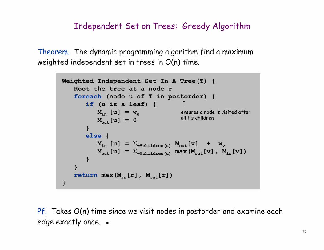
Independent Set on Trees: Greedy Algorithm

Theorem. The dynamic programming algorithm find a maximum weighted independent set in trees in O(n) time. Pf. Takes O(n) time since we visit nodes in postorder and examine each edge exactly once. ▪

Weighted-Independent-Set-In-A-Tree(T) { Root the tree at a node r foreach (node u of T in postorder) { if (u is a leaf) { Min [u] = wu Mout[u] = 0 } else { Min [u] = Σv∈children(u) Mout[v] + wv Mout[u] = Σv∈children(u) max(Mout[v], Min[v]) } } return max(Min[r], Mout[r]) }

ensures a node is visited after all its children

82

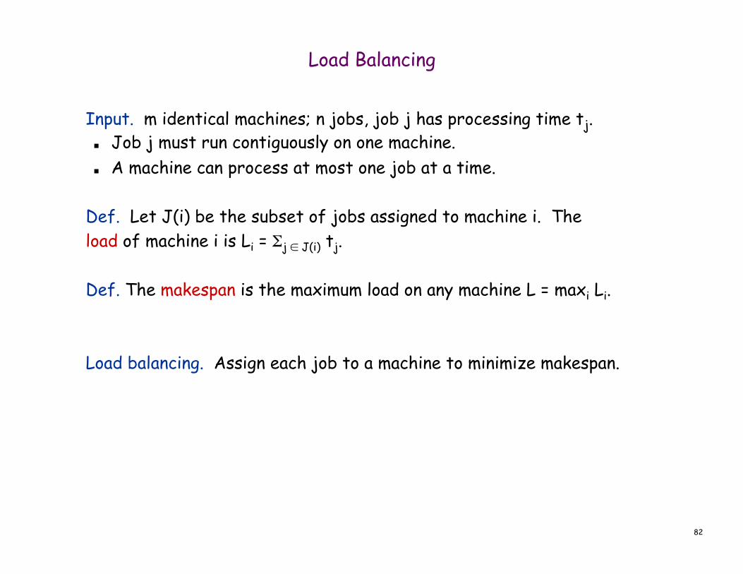
Load Balancing

Input. m identical machines; n jobs, job j has processing time tj. ■  Job j must run contiguously on one machine. ■  A machine can process at most one job at a time.

Def. Let J(i) be the subset of jobs assigned to machine i. The load of machine i is Li = Σj ∈ J(i) tj.

Def. The makespan is the maximum load on any machine L = maxi Li.

Load balancing. Assign each job to a machine to minimize makespan.

83

List-scheduling algorithm. ■  Consider n jobs in some fixed order. ■  Assign job j to machine whose load is smallest so far.

Implementation. O(n log n) using a priority queue.

Load Balancing: List Scheduling

List-Scheduling(m, n, t1,t2,…,tn) { for i = 1 to m { Li ← 0 J(i) ← φ } for j = 1 to n { i = argmink Lk J(i) ← J(i) ∪ {j} Li ← Li + tj } }

jobs assigned to machine i load on machine i

machine i has smallest load assign job j to machine i update load of machine i

84

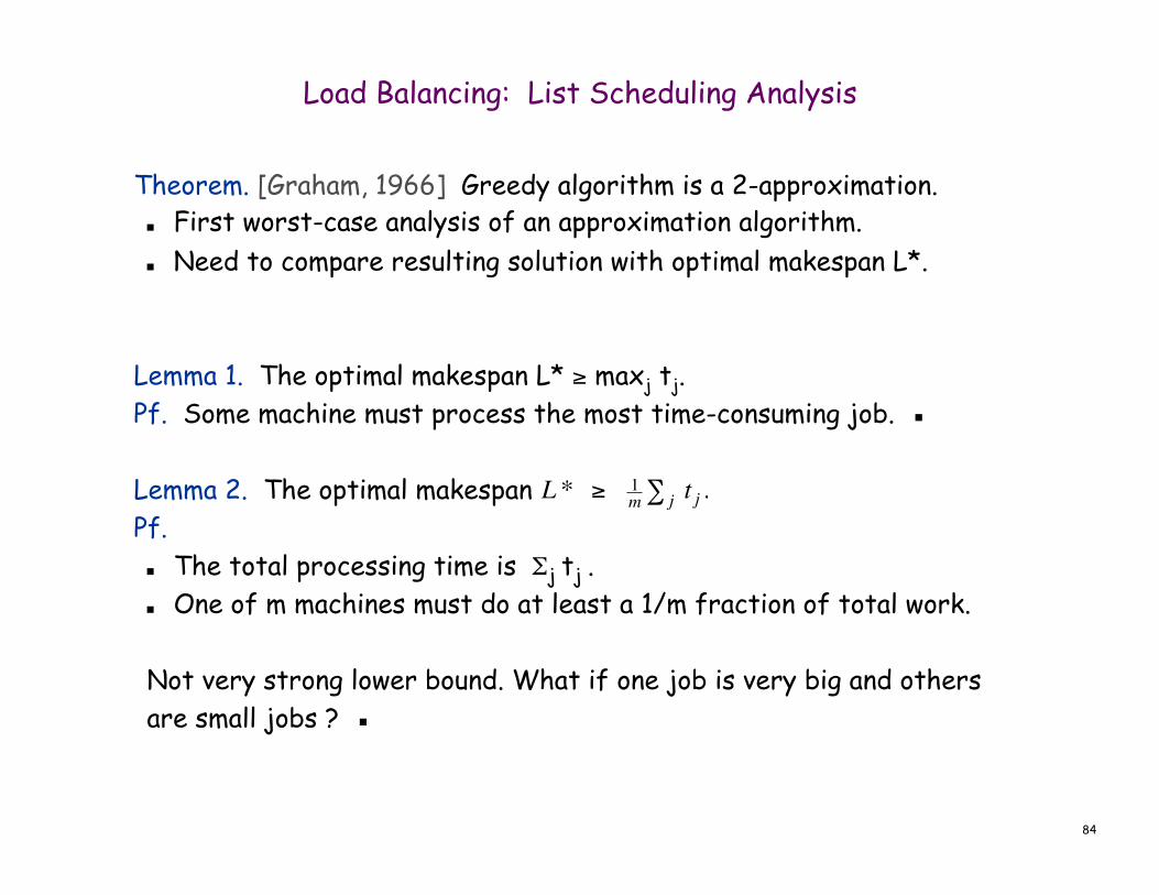
Load Balancing: List Scheduling Analysis

Theorem. [Graham, 1966] Greedy algorithm is a 2-approximation. ■  First worst-case analysis of an approximation algorithm. ■  Need to compare resulting solution with optimal makespan L*.

Lemma 1. The optimal makespan L* ≥ maxj tj. Pf. Some machine must process the most time-consuming job. ▪ Lemma 2. The optimal makespan Pf. ■  The total processing time is Σj tj . ■  One of m machines must do at least a 1/m fraction of total work. Not very strong lower bound. What if one job is very big and others are small jobs ? ▪

€

L * ≥ 1m t jj∑ .

85

Load Balancing: List Scheduling Analysis

Theorem. Greedy algorithm is a 2-approximation. Pf. Consider load Li of bottleneck machine i. ■  Let j be last job scheduled on machine i. ■  When job j assigned to machine i, i had smallest load. Its load

before assignment is Li - tj ⇒ Li - tj ≤ Lk for all 1 ≤ k ≤ m.

j

0 L = Li Li - tj

machine i

blue jobs scheduled before j

86

Load Balancing: List Scheduling Analysis

Theorem. Greedy algorithm is a 2-approximation. Pf. Consider load Li of bottleneck machine i. ■  Let j be last job scheduled on machine i. ■  When job j assigned to machine i, i had smallest load. Its load

before assignment is Li - tj ⇒ Li - tj ≤ Lk for all 1 ≤ k ≤ m. ■  Sum inequalities over all k and divide by m:

■  Now ▪

■  The solution attained by the greedy algorithm is less 2 times the optimal solution

Li − t j ≤ 1m Lkk∑

= 1m t jj∑

≤ L*

€

Li = (Li − t j )≤ L*

+ t j

≤ L*

≤ 2L *.

Lemma 1

Lemma 2

87

Load Balancing: List Scheduling Analysis

Q. Is our analysis tight? A. Essentially yes.

Ex: m machines, m(m-1) jobs length 1 jobs, one job of length m

machine 2 idle machine 3 idle machine 4 idle machine 5 idle machine 6 idle machine 7 idle machine 8 idle machine 9 idle machine 10 idle

list scheduling makespan = 19

m = 10

88

Load Balancing: List Scheduling Analysis

Q. Is our analysis tight? A. Essentially yes.

Ex: m machines, m(m-1) jobs length 1 jobs, one job of length m

m = 10

optimal makespan = 10

89

Load Balancing: LPT Rule

Longest processing time (LPT). Sort n jobs in descending order of processing time, and then run list scheduling algorithm.

LPT-List-Scheduling(m, n, t1,t2,…,tn) { Sort jobs so that t1 ≥ t2 ≥ … ≥ tn for i = 1 to m { Li ← 0 J(i) ← φ } for j = 1 to n { i = argmink Lk J(i) ← J(i) ∪ {j} Li ← Li + tj } }

jobs assigned to machine i load on machine i

machine i has smallest load assign job j to machine i

update load of machine i

90

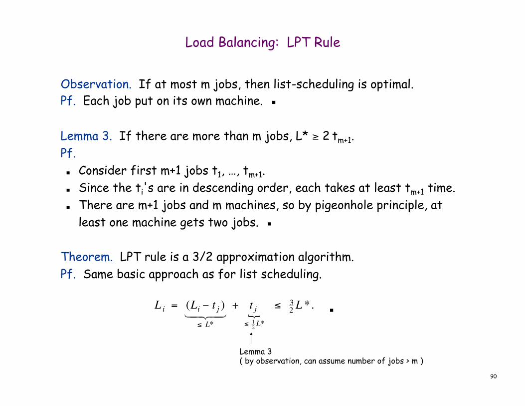
Load Balancing: LPT Rule

Observation. If at most m jobs, then list-scheduling is optimal. Pf. Each job put on its own machine. ▪ Lemma 3. If there are more than m jobs, L* ≥ 2 tm+1. Pf. ■  Consider first m+1 jobs t1, …, tm+1. ■  Since the ti's are in descending order, each takes at least tm+1 time. ■  There are m+1 jobs and m machines, so by pigeonhole principle, at

least one machine gets two jobs. ▪

Theorem. LPT rule is a 3/2 approximation algorithm. Pf. Same basic approach as for list scheduling.

▪

€

Li = (Li − t j )≤ L*

+ t j

≤ 12 L*

≤ 32 L *.

Lemma 3 ( by observation, can assume number of jobs > m )

91

Coping With NP-Hardness

Q. Suppose I need to solve an NP-hard problem. What should I do? A. Theory says you're unlikely to find poly-time algorithm.

Must sacrifice one of three desired features. ■  Solve problem to optimality. ■  Solve problem in polynomial time. ■  Solve arbitrary instances of the problem.