REVIEW FOR R

Middle East Technical University Department of Statistics 2017-18 Spring Semester STAT 292 Statistical Computing II

Created by Ozancan Özdemir for students who take Statistical Computing.

REVIEW FOR R

R Programming

What is R?

R is a high-level computer language and environment for statistics and graphics.

Performing a variety of simple and advanced statistical methods.

Producing high quality graphics.

R is a computer language so we can write new functions that extends R's uses.

R was initially written by Ross Ihaka and Robert Gentleman at the Department of

Statistics of the University of Auckland in Auckland, New Zealand (hence the name).

R is a free open source software maintained by several contributors. Including an \R Core

Team" of 17 programmers who are responsible for modifying the R source code.

Most universities and jobs require or at least prefer that you know R

The official R home page is http://www.R-project.org

Downloading and Installing R

To download R for the first time (to update the version, see bellows)

Go to http://www.R-project.org

Click on Download CRAN (CRAN: Comprehensive R Archive Network)

Select a country geographically nearby Turkey.

Click on Download R for Windows, select base.

Click on Download R 3.x.x for Windows, select “Save”.

To install R

Go to the folder at which the exe file is downloaded.

Click on that then NEXT, NEXT, NEXT and FINISH.

http://www.r-project.org/

http://www.r-project.org/



Downloading and Installing R Studio

To download R for the first time (to update the version, see bellows)

Go to https://www.rstudio.com/

Click on Download

Click on Download button under R Studio (Open Source) title.

Note that you must install R, before installing R Studio!

Getting help and Libraries

To get help on a specific command, e.g. plot, type on R ?plot

If you are not sure of the exact form of the command

Either go to help menu on R console or type on R console ??plot

Either way, a help window will pop up including a list of all the commands having the

word plot. e.g one of them is boot::glm.diag.plots. This expression consists of two parts:

boot and glm.diag.plots. Every command is contained in a library. The first term, boot, is

the name of the library. The second term, glm.diag.plots, is the name of plot.

To get help on glm.diag.plots: type on R window library(boot). Then type

?glm.diag.plots

If the library (i.e package) is not preloaded, you will get an error message when you type

library(boot). To load it, go to packages on the menu in the R console. You need your

computer to be connected to the Internet for loading up the packages.

Alternatively, you can use install.packages function. e.g

install.packages(“boot”)



Preliminaries

R console: That’s the window where you type your commands. There is a sign on the left

hand side of each line. Next to it, you type your command.

R Programming

R Studio



How to assign values to variables

> x<-2

> x=2

What to name variables

1. Name should start with a letter.

2. Name can continue with letters, numbers, dot or underline characters.

3. Case is important. That is a and A are different names.

Where to write your commands

You can write your commands on the R console window or in a simple editor such as

Notepad or R script.

Basic Commands

ls() to see which objects and functions are saved in the workspace

rm(‘a’) deletes the object a from the workspace.

rm(list=ls()) deletes everything in the workspace.

dir() to see the contents of the folder you are in

q() to exit the R console.

# helps you to add your explanation. e.g x<-2 #the value of x equals to 2

Ctrl+L deletes codes on the console window.

Ctrl+R or Ctrl+Enter run the codes on the editor.

You can repeat the previously written comands by using arrow keys.

Working Directory

Working directory is one of the basic and important point in R and R Studio. Any file that

you want to work on or load must be under your current folder. There are two ways to

change working directory in R. The needed information about these ways are given

below.



R Programming

First way to type following codes on R console.

> getwd() #You get the working directory

[1] "C:/Users/Ozancan/Documents"

> setwd("C:/Users/Ozancan/Desktop")

You can follow way shown in the following pictures.

First, select file and click on change directory option. After clicking on change directory

option, the following screen is shown.

Then, you can select your working directory.



R Studio

First way to type following codes on R console.

> getwd() #You get the working directory

[1] "C:/Users/Ozancan/Documents"

> setwd("C:/Users/Ozancan/Desktop")

You can follow way shown in the following pictures.

First, click on the three dots marked with yellow.

Then, you can select your working directory.



BASIC OPERATIONS

Mathematical Operators

R and R Studio can be considered as a powerful calculator. Some basic examples are given

below.

> 3+5

[1] 8

> 7*8

[1] 56

> 88/2

[1] 44

> 5^2 #taking the square

[1] 25

> a = 3

> b = a^2

> print(b)

[1] 9

> log(15) #ln15

[1] 2.70805

> log10(1000) #log10 is logarithm base 10

[1] 3

> exp(12) #e^12

[1] 162754.8

> 31%%7 # 31 (mod 7), i.e., the remainder after division of 31 by 7

[1] 3

Comparison Operators

These operators are frequently used for data subseting, loops and writing functions.

> greater than

< less than

>= greater than or equals

<= less than or equals

= = equality

~ = inequality

| Or

& And

> 3>5

[1] FALSE

> 3<5&6>7

[1] FALSE

> 3<5|6>7

[1] TRUE



Creating a sequence in R

A sequence is an enumerated collection of objects in which repetitions are allowed. Like a set, it

contains members The number of elements (possibly infinite) is called the length of the

sequence.

To form a sequence use the command seq or ‘:’. e.g

> a=1:20

> a

[1] 1 2 3 4 5 6 7 8 9 10 11 12 13 14 15 16 17 18 19 20

> a=seq(5,25)

> a

[1] 5 6 7 8 9 10 11 12 13 14 15 16 17 18 19 20 21 22 23 24 25

> z=seq(1,20,2) #the last number in paranthesis shows the amount of increment

> z

[1] 1 3 5 7 9 11 13 15 17 19

To repeat the sequence of numbers use the command rep. e.g

> rep(z,2)

[1] 1 3 5 7 9 11 13 15 17 19 1 3 5 7 9 11 13 15 17 19

> rep(seq(1,9,3),4)

[1] 1 4 7 1 4 7 1 4 7 1 4

> rep(seq(1,9,3),each=4)

[1] 1 1 1 1 4 4 4 4 7 7 7 7

Arrays and Matrices

To construct a vector and define it as an object named v

> v=c(1.2,3.5,.79,25)

> v

[1] 1.20 3.50 0.79 25.00

To extract the rth entry of the vector use v[r] where r is any number > v[2]

[1] 3.5

> v[c(1,2)]

[1] 1.2 3.5

Length show the length of the vector > length(v)

[1] 4



The logical operators are used to extract elements from array according to some criteria.

e.g > v=c(1.2,3.5,.79,25)

> v[v>2.3]

[1] 3.5 25.0

> v[v>20 & v<30]

[1] 25

> v[v==1.2 | v<1]

[1] 1.20 0.79

By using c (combine command), you can create an array that contains only characters. > odtu=c("odtu","1956","yılında","kuruldu")

> odtu

[1] "odtu" "1956" "yilinda" "kuruldu"

To extract entry from such an array > odtu[odtu=="yılında"]

[1] "yilinda"

You can give names to elements in R by using names command.

> names(v)=c("1stentry","2ndentry","3rdentry","4thentry")

> v

1stentry 2ndentry 3rdentry 4thentry

1.20 3.50 0.79 25.00

To extract elements from arrays with element names. > v["1stentry"]

1stentry

1.2

> v[c("1stentry","2ndentry")]

1stentry 2ndentry

1.2 3.5

To construct a matrix of size I by J and define as an object and called mat. > mat=matrix(c(1,2,3,4,5,6),ncol=2)

> mat

[,1] [,2]

[1,] 1 4

[2,] 2 5

[3,] 3 6

Another way to construct a matrix; > mat2=matrix(c(1,2,3,4,5,6),3,2)#3 represents number of row, 2 represents

number of column

> mat2

[,1] [,2]

[1,] 1 4

[2,] 2 5

[3,] 3 6



To extract the e.g 2,1 th entry of matrix of mat use mat[2,1] > mat[2,1]

[1] 2

We can assign names to rows and columns of a matrix. e.g Consider the matrix defined

above.

> rownames(mat)=c("istanbul","beyoğlu","taksim")

> colnames(mat)=c("galata","saray")

> mat

galata saray

istanbul 1 4

beyoğlu 2 5

taksim 3 6

> mat["istanbul","galata"]

[1] 1

You can find out the dimension of any matrix with dim command. > mat

[,1] [,2]

[1,] 1 4

[2,] 2 5

[3,] 3 6

> dim(mat)#dimension of the matrix

[1] 3 2

If you wish to obtain only row number of any matrix, you have to use nrow command.

On the other hand, if you want to see only column number of any matrix, it is enough

to type ncol command.

> nrow(mat)#number of rows for mat that is the name of matrix you defined.

[1] 3

> ncol(mat)#number of columns for mat that is the name of matrix you defined.

[1] 2



More details about matrices

> A <- matrix(c( 6, 1,+ 0, -3,-1, 2),3, 2, byrow = TRUE)

> B <- matrix(c( 4, 2,0, 1,-5, -1),3, 2, byrow = TRUE)

> A

[,1] [,2]

[1,] 6 1

[2,] 0 -3

[3,] -1 2

> B

[,1] [,2]

[1,] 4 2

[2,] 0 1

[3,] -5 -1

> A + B #summation of two matrices

[,1] [,2]

[1,] 10 3

[2,] 0 -2

[3,] -6 1

> A – B #subtraction of two matrices

[,1] [,2]

[1,] 2 -1

[2,] 0 -4

[3,] 4 3

> A * B # this is component-by-component multiplication, not matrix multiplication

[,1] [,2]

[1,] 24 2

[2,] 0 -3

[3,] 5 -2

> t(A) #take the transpose of the matrix

[,1] [,2] [,3]

[1,] 6 0 -1

[2,] 1 -3 2

> C<-matrix(c(2,4,5,6),nrow=2)

> C

[,1] [,2]

[1,] 2 5

[2,] 4 6

> A%*%C #the matrix multiplication

[,1] [,2]

[1,] 16 36

[2,] -12 -18

[3,] 6 7

> solve (C) #take the inverse of the matrix

[,1] [,2]

[1,] -0.75 0.625

[2,] 0.50 -0.250



Adding/Deleting Elements of Vectors and Matrices: Technically, vectors and matrices are of fixed

length and dimensions. However, they can be reassigned.

> x <- c(12,5,13,16,8)

> x <- c(x,20) # append 20

> x

[1] 12 5 13 16 8 20

> x <- c(x[1:3],20,x[4:6]) # insert 20

> x

[1] 12 5 13 20 16 8 20

> x <- x[-2:-4]# delete elements 2 through 4

> x

[1] 12 16 8 20

The rbind() and cbind() functions enable one to add rows or columns to a matrix.

> one=c(1,1,1,1)

> one

[1] 1 1 1 1

> z=matrix(c(1,2,3,4,1,1,0,0,1,0,1,0),ncol=3)

> z

[,1] [,2] [,3]

[1,] 1 1 1

[2,] 2 1 0

[3,] 3 0 1

[4,] 4 0 0

> cbind(one,z) #"combine vector and matrix as column

one

[1,] 1 1 1 1

[2,] 1 2 1 0

[3,] 1 3 0 1

[4,] 1 4 0 0

> q=rbind(c(1,2),c(3,4))#combine vector and matrix as row

> q

[,1] [,2]

[1,] 1 2

[2,] 3 4



To delete entry from matrices or vectors – (minus) sign is used. > z=matrix(c(1,2,3,4,1,1,0,0,1,0,1,0),ncol=3)

> z

[,1] [,2] [,3]

[1,] 1 1 1

[2,] 2 1 0

[3,] 3 0 1

[4,] 4 0 0

> z[-1,] #deleting first row

[,1] [,2] [,3]

[1,] 2 1 0

[2,] 3 0 1

[3,] 4 0 0

> z[-c(1,2),]#deleting first and second row. To delete more than one row,

# use c (combine) command

[,1] [,2] [,3]

[1,] 3 0 1

[2,] 4 0 0

> z[,-1]#deleting first column

[,1] [,2]

[1,] 1 1

[2,] 1 0

[3,] 0 1

[4,] 0 0

> z[,-c(1,2)]#deleting first and second column. To delete more than one row, use

# c (combine) command

[1] 1 0 1 0

Swirl library in R – Learn R in R

The swirl R package makes it fun and easy to learn R programming and data science. If you are

new to R, have no fear. On this page, we’ll walk you through each of the steps required to begin

using swirl.

In order to run swirl, you must have R 3.1.0 or later installed on your computer.

Step 1: Get R and R Studio

Step 2: Install Swirl : > install.packages("swirl")

Step 3: Start Swirl: >library(swirl)#call the swirl

>swirl() #start swirl

Step 4: Install an interactive course

The first time you start swirl, you'll be prompted to install a course. You can either install one of

the recommended courses or visit http://swirlstats.com/students.html for more options. There are

even more courses available from the Swirl Course Network.

http://swirlstats.com/students.html



If you'd like to install a course that is not part of our course repository, type ?InstallCourses

at the R prompt for a list of functions that will help you do so.

Reading Data Sets in R

Before we move on and discover how to load your data into R, it might be useful to go over

following checklist that will make it easier to import the data correctly into R:

If you work with spreadsheets, the first row is usually reserved for the header, while the

first column is used to identify the sampling unit;

Avoid names, values or fields with blank spaces, otherwise each word will be interpreted

as a separate variable, resulting in errors that are related to the number of elements per

line in your data set;

If you want to concatenate words, inserting a . in between to words instead of a space;

Short names are prefered over longer names;

Try to avoid using names that contain symbols such as ?, $,%, ^, &, *, (, ),-,#, ?,,,<,>, /, |

, \, [ ,] ,{, and };

Delete any comments that you have made in your Excel file to avoid extra columns or

NA’s to be added to your file; and make sure that any missing values in your data set are

indicated with NA.

Preparing your R workspace

In general, when you read the data set, your data file MUST BE in your working

directory. If you remember how to do it, OK. Otherwise, please look at the previous

recitation or reminder at the beginning of the recitation.

Loading data set being available in R

R and R Studio includes many data sets. In order to load such a data set, you have to type the

name of data set on R console. To see the list of the data sets, you can visit the following page.

https://stat.ethz.ch/R-manual/R-devel/library/datasets/html/00Index.html

> cars

> AirPassengers

> mtcar

https://stat.ethz.ch/R-manual/R-devel/library/datasets/html/00Index.html



Read TXT files with read.table()

If you have a .txt or a tab-delimited text file, you can easily import it with the basic R function

read.table().

If the variables in your data set have

column names.

> read.table("drug.txt",header=T)

drug math

1 1.17 78.93

2 2.97 58.20

3 3.26 67.47

4 4.69 37.47

5 5.83 45.65

6 6.00 32.92

7 6.41 29.97

If the variables in your data set do not

have column names.

> read.table("drug1.txt",header=F)

V1 V2

1 1.17 78.93

2 2.97 58.20

3 3.26 67.47

4 4.69 37.47

5 5.83 45.65

6 6.00 32.92

7 6.41 29.97

Read CSV Excel Files into R

If you have a file that separates the values with a , or ; you usually are dealing with a .csv file.

To successfully load this file into R, you can use the read.table() function in which you specify

the separator character, or you can use the read.csv() or read.csv2() functions. The former

function is used if the separator is a ,, the latter if ; is used to separate the values in your data file.

Remember that the read.csv() as well as the read.csv2() function are almost identical to the

read.table() function

> yates1=read.table("yates.csv",sep=",",header=T)

> head(yates1) #shows some first observation of the data set, you can use it

any time

Block Trt Yield

1 1 2 51.50

2 1 7 36.75

3 1 11 21.00

4 1 15 41.56

5 1 19 22.25

6 2 1 50.75



> yates2=read.csv("yates.csv",header=T)

> head(yates2)

Block Trt Yield

1 1 2 51.50

2 1 7 36.75

3 1 11 21.00

4 1 15 41.56

5 1 19 22.25

6 2 1 50.75

read.delim() for Delimited Files

The read.delim function is typically used to read in delimited text files, where data is organized

in a data matrix with rows representing cases and columns representing variables.

> d=read.delim("annual.txt", header=TRUE, sep="\t")

> head(d)

month avgHigh season schoolIn

1 Jan 38 Winter yes

2 Feb 41 Winter yes

3 Mar 47 Spring yes

4 Apr 56 Spring yes

5 May 69 Spring yes

6 Jun 81 Summer no

sep="\t" tells R that the file is tab-delimited (use " " for space delimited and "," for

comma delimited)

In addition to them, there are many type of data set and there are many ways to read these data

set into R and R Studio. You can learn these by searching on the internet.

Some Built-in Functions

There are many built-in functions in R. Here are some of them. Assume we have the following x

vector. > x=c(1,9,0,5,1,9,5,6)

> which(x==6)#shows the location of 6 in the vector of x

[1] 8

> which.max(x)#shows the location of the maximum element of vector of x

[1] 2

> length(x) #to see the length of the vector

[1] 8

> max(x) #maximum value of a vector

[1] 9

> min(x) #minimum value of a vector

[1] 0

> range(x)#minimum and maximum values of vectors

[1] 0 9



> sum(x)#the summation of all elements of a vector

[1] 36

> cumsum(x)#cumulative sum of vector

[1] 1 10 10 15 16 25 30 36

> mean(x)#mean of the vector

[1] 4.5

> median(x)#median of the vector

[1] 5

> var(x)#variance of vector

[1] 12.57143

> sd(x)#standard deviation of the vector

[1] 3.545621

> sort(x)#sort in increasing order

[1] 0 1 1 5 5 6 9 9

> sort(x,decreasing = T)#sort in decreasing order

[1] 9 9 6 5 5 1 1 0

> diff(x)#take the difference of ith and (i+1)th element

[1] 8 -9 5 -4 8 -4 1

If we have a matrix, > x=matrix(c(2,4,6,1,2,3,3,6,9),3,3)

> x

[,1] [,2] [,3]

[1,] 2 1 3

[2,] 4 2 6

[3,] 6 3 9

> which(x==6)#shows the location of 6 in the matrix as vector x

[1] 3 8

> which.max(x)#shows the location of the maximum element of the matrix as vec

tor x

[1] 9

> length(x) #to see the length of the matrix as vector

[1] 9

> max(x) #maximum value of the matrix as vector

[1] 9

> min(x) #minimum value of the matrix as vector

[1] 1

> range(x)#minimum and maximum values of the matrix as vector

[1] 1 9

> sum(x)#the summation of all elements of the matrix as vector

[1] 36

> cumsum(x)#cumulative sum of the matrix as vector

[1] 2 6 12 13 15 18 21 27 36

> mean(x)#mean of the matrix as vector

[1] 4

> median(x)#median of the matrix as vector

[1] 3

> sd(x)#standard deviation of the matrix as vector

[1] 2.54951

> sort(x)#sort in increasing the matrix as vector

[1] 1 2 2 3 3 4 6 6 9

> sort(x,decreasing = T)#sort in decreasing order

[1] 9 6 6 4 3 3 2 2 1



> diff(x)#take the difference of i,j th and (i+1,j)th element of the matrix

[,1] [,2] [,3]

[1,] 2 1 3

[2,] 2 1 3

Data Frame

A data frame in R combines features of vectors, matrices, and lists. Like vectors, data frames

must have the same kind of data in each column. Like matrices, data frames have both rows and

columns. And like lists, data frames allow the user to have a combination of numeric, character,

and logical data. You can think of a data frame in the same way you would think of a data set in

a statistics program or a worksheet in Excel or some other spreadsheet program.

Creating a Data Frame from Vectors

> people <-c("Kim","Bob","Ted","Sue","Liz","Amanada","Tricia","Johnathan","Lu

is","Isabel")

> gender<-c("m","m","m","f","f","f","f","f","m","f")

> scores <-c(17,19,24,25,16,15,23,24,29,17)

> quiz_scores <- data.frame(people,gender,scores) #to create a data frame

> quiz_scores

people gender scores

1 Kim m 17

2 Bob m 19

3 Ted m 24

4 Sue f 25

5 Liz f 16

6 Amanada f 15

7 Tricia f 23

8 Johnathan f 24

9 Luis m 29

10 Isabel f 17

We can obtain individual columns by using the column index in square brackets. We can

also employ the data frame name followed by a $ sign and the column name.

> quiz_scores[2]

scores

1 17

2 19

3 24

4 25

5 16

6 15

7 23

8 24

9 29

10 17



> quiz_scores$scores #mostly used version

[1] 17 19 24 25 16 15 23 24 29 17

> attach(quiz_scores)

> scores

[1] 17 19 24 25 16 15 23 24 29 17

Changing class of the object

Suppose you read your data set into R or you have an object created in R, and you wish to

change the class of it.

> x=1:5

> y=6:10

> z=c(x,y)

> class(z)#to find out the class of the object

[1] "integer"

> z=as.data.frame(z)

> class(z)

[1] "data.frame"

> z1=as.matrix(z)

> class(z1)

[1] "matrix"

Accessing data from Data Frame

> quiz_scores$people

[1] Kim Bob Ted Sue Liz Amanada Tricia Johnathan Luis Isabel

Levels: Amanada Bob Isabel Johnathan Kim Liz Luis Sue Ted Tricia

> quiz_scores$scores>15

[1] TRUE TRUE TRUE TRUE TRUE FALSE TRUE TRUE TRUE TRUE

> quiz_scores$scores[quiz_scores$scores>15] #to see grades greater than 15

[1] 17 19 24 25 16 23 24 29 17

> quiz_scores[quiz_scores[,"scores"]>15,] #to see grades greater than 15 and

corresponding other variables


1 Kim m 17

2 Bob m 19

3 Ted m 24

4 Sue f 25

5 Liz f 16

7 Tricia f 23

8 Johnathan f 24

9 Luis m 29

10 Isabel f 17

> quiz_scores$scores[quiz_scores$gender=="f"]#to see grades for female

students

[1] 25 16 15 23 24 17



> quiz_scores[quiz_scores[,"gender"]=="f",]#to see grades for female students

and corresponding other variables


4 Sue f 25

5 Liz f 16

6 Amanada f 15

7 Tricia f 23

8 Johnathan f 24

10 Isabel f 17

Data Subsetting > data=read.table("data.txt",header=T) > head(data) nation birth_rate pci pop mortality_rate 1 Venezuela 46.4 392 0.40 68.5 2 Mexico 45.7 118 0.61 87.8 3 Ecuador 45.3 44 0.53 115.8 4 Colombia 38.6 158 0.53 106.8 5 Ceylon 37.2 81 0.53 71.6 6 PuertoRico 35.0 374 0.37 60.2 > class(data) [1] "data.frame" > dim(data) [1] 29 5

Assume we want to construct a new matrix with the first 10 rows of data data[1:10,]

Assume we want to construct a new matrix with the 1 st , 3 nd ,12 th , and 15 th rows of

data data[c(1,3,12,15),]

Assume we want to construct a new matrix same as data but without the 4th row of data data[-4,]

Assume we want to construct a new matrix same as data but without the 3rd,5th,12nd and

27th row of the data data[-c(3,5,12,27),]

Assume we want to construct a new matrix same as data but without pci information data[,-3]

Assume we want to construct a new matrix same as data but without pci and mortality

rate information data[,-c(3,5)]

Assume we want to confine the analysis only to birth rate which are at least 25 data[data$birth_rate>=25,] OR data[data[,2]>=25,]

Assume we want to include only the nations whose mortality rate given is between 80 and

120 data[data$mortality_rate>=80&data$mortality_rate<=120,]

data[data[,5]>=80&data[,5]<=120,]

Assume we want to include only the nations whose population per income equals to either

0.53 or 0.3 data[data$pop==0.53|data$pop==0.3,]



Graphics: Graphics is a great strength of R. The graphics package is part of the standard

distribution and contains many useful functions for creating a variety of graphic displays.

Scatter Plot: Scatter plots can help you identify the relationship between two data samples. A

scatter plot is a simple plot of one variable against another. In order to draw a scatter plot, the

following command is used

> plot(x)#draw the scatter plot of random variable x

> plot(x,y)##draw the scatter plot of random variables x and y

> x=c(0.25, 0.295, 0.473, 0.476, 0.512,0.588, 0.629, 0.648, 0.722, 0.844)

> y=c(0.00102, 0.271, 0.378, 0.478, 0.495, 0.663, 0.68, 0.778, 0.948, 0.975)

> plot(x)#Draw scatter plot of x

> plot(x,y)#Draw scatter plot of x and y



If you draw a scatter or line plot, note that your x variable should be arranged in an order.

In previous example, the elements in the vector x is arranged in an order. If they are not ordered,

it is possible to use sort command to obtain an ordered vector.

> x=c(0.25, 0.473, 0.476, 0.844 ,0.629, 0.588, 0.512, 0.648, 0.722,0.295)

> y=c(0.00102, 0.271, 0.378, 0.478, 0.495, 0.663, 0.68, 0.778, 0.948, 0.975)

> plot(x,y) #if you do not use sort

> plot(sort(x),y) # if you use sort



Adding Title and Labels and Other Manupulations

> head(cars)

speed dist

1 4 2

2 4 10

3 7 4

4 7 22

5 8 16

6 9 10

> plot(cars$speed,cars$dist)

> #main command is used to add title into your plot

> #xlab command is used to change the name of x label

> #ylab command is used to change the name of y label

> plot(x, main="The Title", xlab="X-axis Label", ylab="Y-axis Label")

Change the plot character

> plot(x, main="The Title", xlab="X-axis Label", ylab="Y-axis Label",pch=12)



Changing the color of points or figures in the plot

In order to see the color index, you can visit,

https://www.statmethods.net/advgraphs/parameters.html

> plot(x, main="The Title", xlab="X-axis Label", ylab="Y-axis Label",pch=6, col=18)#col command help us to arrange the color of the points

> grid() #to add grid

https://www.statmethods.net/advgraphs/parameters.html



Add Lines to Your Plot

abline(a = NULL, b = NULL, h = NULL, v = NULL...)

a, b the intercept and slope, single values.

h the y-value(s) for horizontal line(s).

v the x-value(s) for vertical line(s).

> abline(h=0.6,v=4)

> plot(x, main="The Title", xlab="X-axis Label", ylab="Y-axis Label",pch=6,

col=18)#col command help us to arrange the color of the points

> lines(y) #you can add y variables as line in the plot



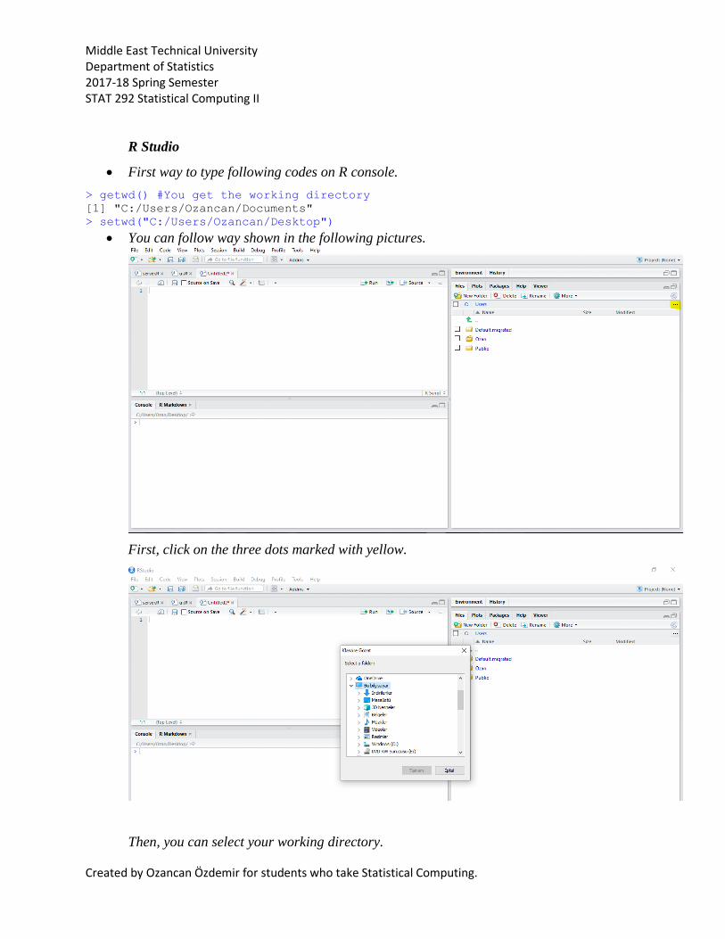
Showing more than one plot in one window

> par(mfrow=c(1,2)) #where c(nofrow,nofcolumn)

> plot(x, main="The Title", xlab="X-axis Label", ylab="Y-axis Label",pch=12)

> plot(x, main="The Title", xlab="X-axis Label", ylab="Y-axis Label",pch=6,col=18)

#col command help us to arrange the color of the points

#after using par() command, when you draw a new plot please do not forget to close

your window

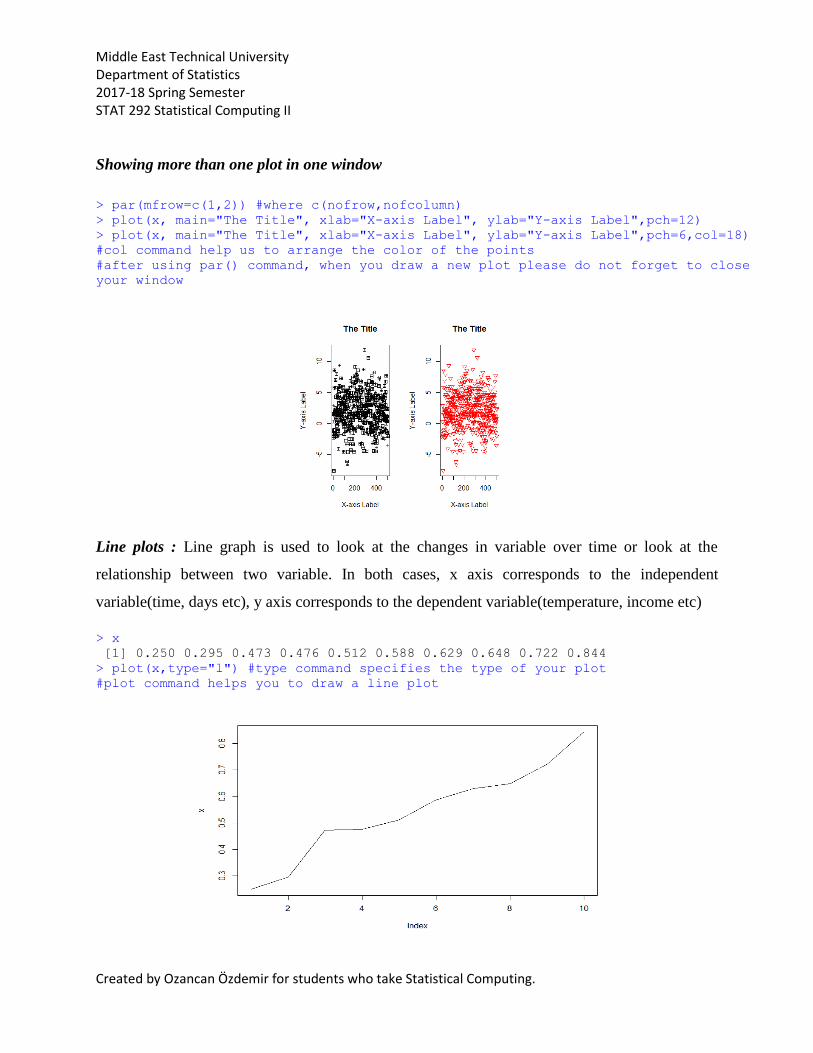
Line plots : Line graph is used to look at the changes in variable over time or look at the

relationship between two variable. In both cases, x axis corresponds to the independent

variable(time, days etc), y axis corresponds to the dependent variable(temperature, income etc)

> x

[1] 0.250 0.295 0.473 0.476 0.512 0.588 0.629 0.648 0.722 0.844

> plot(x,type="l") #type command specifies the type of your plot

#plot command helps you to draw a line plot



In order to add label names, titles and change the line color, you can use the previous

commands which are xlab, ylab, main etc.

> head(cars)

speed dist

1 4 2

2 4 10

3 7 4

4 7 22

5 8 16

6 9 10

> attach(cars) #in order to not to use $ sign

> plot(speed,dist,type="l",main="The line plot of speed and distance",xlab="s

peed of the car",ylab="speed of the dist",col=12,lty=2)

> #main->add title

> #xlab and ylab -> add label name

> #col-> change the color of the line

> #More examples on lty:

> #lty= "solid" or lty=1

> #lty= "dashed" or lty=2

> #lty= "dotted" or lty=3

> #lty= "dotdash" or lty=4

> #lty= "longdash" or lty=5

> #lty= "twodash" or lty=6

> grid()#you can add grid

> abline(h=70,v=12)



Bar Plot: A bar chart or bar graph is a chart or graph that presents categorical data with

rectangular bars with heights or lengths proportional to the values that they represent. The

barplot function produces a simple bar chart. It assumes that the heights of your bars are

conveniently stored in a vector.

> head(mtcars)

mpg cyl disp hp drat wt qsec vs am gear carb

Mazda RX4 21.0 6 160 110 3.90 2.620 16.46 0 1 4 4

Mazda RX4 Wag 21.0 6 160 110 3.90 2.875 17.02 0 1 4 4

Datsun 710 22.8 4 108 93 3.85 2.320 18.61 1 1 4 1

Hornet 4 Drive 21.4 6 258 110 3.08 3.215 19.44 1 0 3 1

Hornet Sportabout 18.7 8 360 175 3.15 3.440 17.02 0 0 3 2

Valiant 18.1 6 225 105 2.76 3.460 20.22 1 0 3 1

> counts <- table(mtcars$gear)#table commands helps you to create the

frequency table

> counts

3 4 5

15 12 5

> barplot(counts, main="Car Distribution", xlab="Number of Gears")

You can see also list of colors in R from this pdf file.

http://www.stat.columbia.edu/~tzheng/files/Rcolor.pdf

> barplot(counts, main="Car Distribution", xlab="Number of Gears",ylab="Frequ

ency of Gears",col=c("firebrick","firebrick1","firebrick2"),legend = rownames

(counts))

> #legend command helps you to add small info box

> #also we can use legend=c("3","4","5")

> #to color your bars, you can use col command

http://www.stat.columbia.edu/~tzheng/files/Rcolor.pdf



> barplot(counts, main="Car Distribution", xlab="Number of Gears",ylab="Frequ

ency of Gears",col=c("firebrick","firebrick1","firebrick2"),legend=c("3","4",

"5"))

Histogram

> hist(x)

Quantitative variables often take so many values that a graph of the distribution is clearer if

nearby values are group together. The most common graph of the distribution of one quantitative

variable is a histogram. ( Used for continious type of data)

Symetric (Bell shaped) Right Skewed Left skewed



> #histogram

> #simple histogram

> head(cars)

speed dist

1 4 2

2 4 10

3 7 4

4 7 22

5 8 16

6 9 10

> hist(cars$dist)

> # Colored Histogram with Different Number of Bins

> hist(cars$dist, breaks=12, col="red",xlab="Distance") #breaks used to

arrange number of bin



> # Adding a Normal Curve

> x <- cars$dist

> h<-hist(x, breaks=10, col="red", xlab="Distance",

+ main="Histogram with Normal Curve")

> xfit<-seq(min(x),max(x),length=150)

> yfit<-dnorm(xfit,mean=mean(x),sd=sd(x)) #dnorm->density of normal dist

> yfit <- yfit*diff(h$mids[1:2])*length(x) #mids ->the n cell midpoints.

> lines(xfit, yfit, col="blue", lwd=2)

Box Plot: We use five number summary which are minimum, 1st quartile, median, 3rd quartile

and maximum values of data to draw a box plot.

On each box, the central mark indicates the median, and the bottom and top edges of the box

indicate the 25th and 75th percentiles, respectively. The whiskers extend to the most extreme

data points not considered outliers, and the outliers are plotted individually using the 'o' symbol.

#Simple Box Plot

> head(mtcars)

mpg cyl disp hp drat wt qsec vs am gear carb

Mazda RX4 21.0 6 160 110 3.90 2.620 16.46 0 1 4 4

Mazda RX4 Wag 21.0 6 160 110 3.90 2.875 17.02 0 1 4 4

Datsun 710 22.8 4 108 93 3.85 2.320 18.61 1 1 4 1

Hornet 4 Drive 21.4 6 258 110 3.08 3.215 19.44 1 0 3 1

Hornet Sportabout 18.7 8 360 175 3.15 3.440 17.02 0 0 3 2

Valiant 18.1 6 225 105 2.76 3.460 20.22 1 0 3 1



> boxplot(disp,data=mtcars,main="Box Plot for Disp")

> attach(mtcars) > table(cyl) cyl 4 6 8 11 7 14 > boxplot(mpg~cyl,data=mtcars, main="Car Milage Data", + xlab="Number of Cylinders", ylab="Miles Per Gallon")

> boxplot(mpg~cyl,data=mtcars,main="Car Milage Data",xlab="Number of Cylinder

+s",ylab="Miles Per Gallon",col=c("red","blue","yellow"),names=c("Cyl4","Cyl6

"+,"Cyl8")) #col helps you to add colors into your plot

> #names helps you to change the category names



Pie Chart

Pie charts are created with the function pie(x, labels= ) where x is a non-negative numeric

vector indicating the area of each slice and labels= notes a character vector of names for the

slices.

> # Simple Pie Chart

> slices <- c(10, 12,4, 16, 8)

> lbls <- c("US", "UK", "Australia", "Germany", "France")

> pie(slices, labels = lbls, main="Pie Chart of Countries") #label shows the

label names



> # 3D Exploded Pie Chart

> library(plotrix)

> slices <- c(10, 12, 4, 16, 8)

> lbls <- c("US", "UK", "Australia", "Germany", "France")

> pie3D(slices,labels=lbls,explode=0.1,

+ main="Pie Chart of Countries ")

> #explode helps you to divide your plot

> #if you do not use it, you have only one big slice



Quantile-Quantile Plot (Q-Q Plot): The quantile-quantile (q-q) plot is a graphical technique for

determining whether the variable of interest follows the normal distribution or not. It is also

used to detect outliers in some cases such as regression models.

> x=rnorm(500,2,3) #generate random

number from normal distribution with

mean 2 and sd 3

> qqnorm(x)#draw a qq plot

> qqline(x) #to add normality line

> y=runif(100,2,6)#generate random

number from uniform distribution with

a=2,b=6

> qqnorm(y) #draw a qq plot

> qqline(y)#to add normality line

Handling with Missing Data in R

Missing Data: In statistics, missing data, or missing values, occur when no data value is stored

for the variable in an observation. Missing data are a common occurrence and can have a

significant effect on the conclusions that can be drawn from the data.

There are many types of missing data and different reasons for data being missing. Both issues af

fect the analysis. Some examples are:

In a postal questionnaire survey not all the selected individuals respond;

In a randomised trial, some patients are lost to follow up before the end of the study;

In a multicentre study, some centres do not measure a particular variable;



In a study in which patients are assessed frequently some data are missing at some time p

oints for unknown reasons;

Occasional data values for a variable are missing because some equipment failed;

Some laboratory samples are lost in transit or technically unsatisfactory;

In a magnetic resonance imaging study some very obese patients are excluded as they are

too large for the machine;

In a study assessing quality of life some patients die during the follow up period.

Data often are missing in research in economics, sociology, and political science because

governments choose not to, or fail to, report critical statistics. Sometimes missing values are

caused by the researcher—for example, when data collection is done improperly or mistakes are

made in data entry.

How to deal with it in R?

In general, the missing values are recorded as “NA”, “-99”,”0”,”*”, or nonsense numbers such as

“354564”.

When you start your analysis, you should be aware of having missing value or not. If you have,

then you have to fix this problem with appropriate methods, then you can go further.

> ex <- c(4, 6, 2, NA, 9, 2) # NA is used to show an object is a missing

value in R.

> #Note that, we don't need to use quotation marks to use NA even though it

seems like a character

> ex

[1] 4 6 2 NA 9 2

Testing Missing Values

> is.na(x) # returns TRUE of x is missing

> is.na(ex)

[1] FALSE FALSE FALSE TRUE FALSE FALSE

> #TRUE indicates that the value is missing

> a=c(2,6,5,4)

> na.fail(a)

[1] 2 6 5 4

> ex

[1] 4 6 2 NA 9 2

> na.fail(ex)

Error in na.fail.default(ex) : missing values in object



Recording values to Missing

R reads only “NA” as missing value. Other representations such as “-99”,”*” are not considered

as NA.

> data=read.table("data.txt",header=T)

> data

V1 V2 V3

1 9 4 3

2 5 -99 1

3 -99 2 2

4 -99 -99 -99

5 17 9 8

6 4 2 -99

> data[data==-99]=NA

> data

V1 V2 V3

1 9 4 3

2 5 NA 1

3 NA 2 2

4 NA NA NA

5 17 9 8

6 4 2 NA

Finding out the number of missing values

> length(which(is.na(ex)))

[1] 1

> #We use length, which and is.na command together to find out the number of

missing values

When you have missing values, you cannot do any analysis.

> sum(ex)# Can not gives a result because of the missing case in the vector.

[1] NA

Excluding missing values from analysis

> sum(ex, na.rm = TRUE) # Now, we inform R that there is a missing case

in the vector and want R to ignore it

[1] 23

> #na.rm command help me to remove NA term from the vector.

Removing missing values from data

> ex

[1] 4 6 2 NA 9 2

> ex1=na.omit(ex)

#na.omit deletes NA values in your data.

> ex1

[1] 4 6 2 9 2

attr(,"na.action")



[1] 4

attr(,"class")

[1] "omit"

> sum(ex1)

[1] 23

Missing Imputation .

Fill-in or impute the missing values. Use the rest of the data to predict the missing values.

Simply replacing the missing value of a predictor with the average value of that predictor

is one easy method. Using regression on the other predictors is another possibility. It’s

not clear how much the diagnostics and inference on the filled-in dataset is affected.

Some additional uncertainty is caused by the imputation which needs to be allowed for.

Missing observation correlation. Consider just xi yi pairs with some observations

missing. The means and SDs of x and y can be used in the estimate even when a member

of a pair is missing. An analogous method is available for regression problems.

Maximum likelihood methods can be used assuming the multivariate normality of the

data. The EM algorithm is often used here. We will not explain the details but the idea is

essentially to treat missing values as nuisance parameters.

Most modeling functions in R offer options for dealing with missing values. You can go

beyond pairwise of listwise deletion of missing values through methods such as multiple

imputation. Good implementations that can be accessed through R include Amelia II,

Mice, and mitools.