ReviewReviewInterest Rates and Present Value 

Analysis

Interest RatesInterest Rates

Present Value Analysis

Rate of Return

Continuously Varying Interest Rates

Homework AssignmentsWeek 1  (p. 57) #4.1, 4.2, 4.3Week 2  (pp 58‐62) #4.5, 4.6, 4.8(a), 4.13, 4.20, 4.26(b), 4.28, 4.31, 4.34W k    (   ) #         8Week 3  (pp 15‐19) #1.9, 1.12, 1.13, 1.15, 1.18

(pp 29‐31) #2.2, 2.6, 2.9

Chapter 1Chapter 1Probabilityy

1.1 Probabilities and Events

1.2 Conditional Probability

1.3 Random Variables and Expected Values

1.4 Covariance and Correlation

1.5 Exerciese

Section 1.1Probabilities and EventsProbabilities and Events

4

DefinitionsDefinitionsConsider an experiment.Consider an experiment.

• The sample space, S, is the set of all possible outcomes of the experimentoutcomes of the experiment.

• If there are m possible outcomes of the i t th ill ll b thexperiment then we will generally number them

1 through m. Then S = {1,2, . . . , m}

• When dealing with specific examples, we will usually give more descriptive names to the outcomesoutcomes.

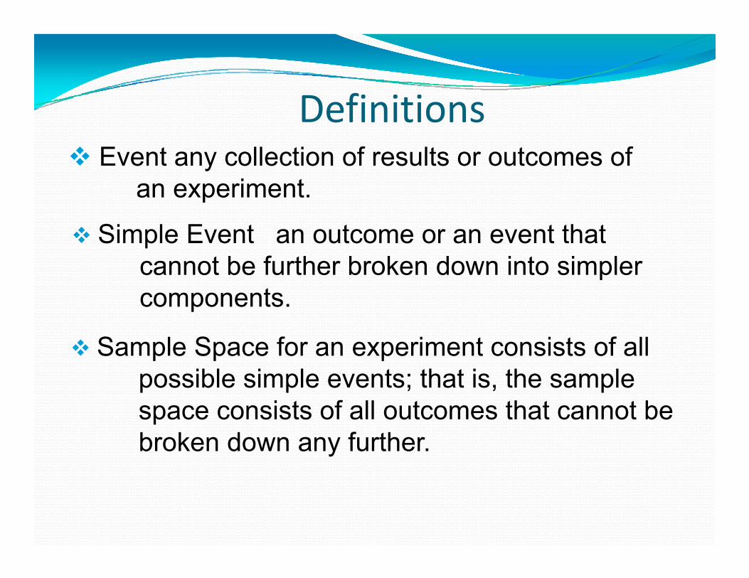
DefinitionsDefinitions Event any collection of results or outcomes of

i tan experiment.

Simple Event an outcome or an event that cannot be further broken down into simpler components.

Sample Space for an experiment consists of all possible simple events; that is, the sample space consists of all outcomes that cannot be broken down any further.

Notation for ProbabilitiesP denotes a probability.

Probabilities

A, B, C, and E denote specific events.

P(A) denotes the probability of event A occurringevent A occurring.

Cl i l A h t P b bilitAssume that a given procedure has n different

Classical Approach to Probabilityg p

simple events and that each of those simple events has an equal chance of occurring. If event A can occur in s of these n ways thenA can occur in s of these n ways, then

N b f W ANumber of Ways A can occur( )Number of different simple events

sP An

Probability Limits

The probability of an event that is certain to

The probability of an impossible event is 0.

The probability of an event that is certain to occur is 1.

F t A th b bilit f A i For any event A, the probability of A is between 0 and 1 inclusive. That is, 0 P(A) 1.

Let S = {1,2, . . . , m}. Let pi be the probability that iLet S   {1,2, . . . , m}. Let pi be the probability that iis the outcome of the experiment. Then

0 1, 1, 2,ip i m

11

m

ii

p

1i

For any event A,For any event A,

( )m

P A p( ) ii A

P A p

( ) 1m

iP S p 1i

Possible ValuesPossible Values for Probabilities

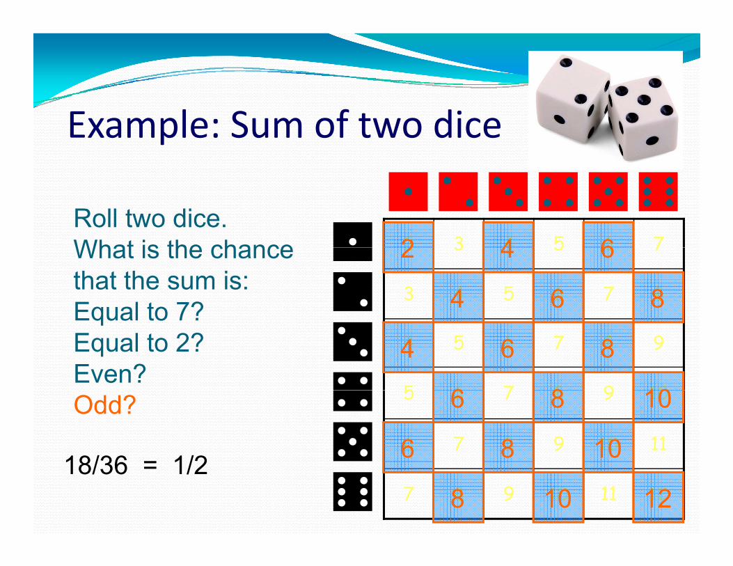
E l S f diExample: Sum of two dice

R ll t di

2 3 4 5 6 7

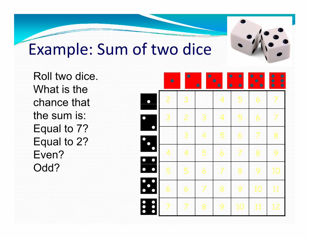
Roll two dice.What is the chance that

3 2 3 4 5 6 7

3 4 5 6 7 8

chance that the sum is:Equal to 7?

3 4 5 6 7 8

4 4 5 6 7 8 9

qEqual to 2? Even? Odd? 5 5 6 7 8 9 10

6 6 7 8 9 10 11

Odd?

7 7 8 9 10 11 12

E l S f diExample: Sum of two dice

R ll t di

2 3 4 5 6 7

Roll two dice.What is the chance that 72 3 4 5 6 7

3 4 5 6 7 8

chance that the sum is:Equal to 7?

7

7

4 5 6 7 8 9

qEqual to 2? Even? Odd?

7

76/36 = 1/6

5 6 7 8 9 10

6 7 8 9 10 11

Odd? 7

7

7 8 9 10 11 127

E l S f diExample: Sum of two dice

2 3 4 5 6 7

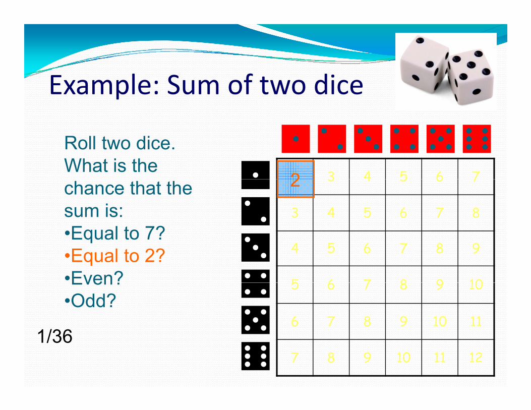
Roll two dice.What is the

22 3 4 5 6 7

3 4 5 6 7 8chance that the sum is:•Equal to 7?

2

4 5 6 7 8 9

5 6 7 8 9 10

•Equal to 7? •Equal to 2?•Even? 5 6 7 8 9 10

6 7 8 9 10 11

Even? •Odd?

1/367 8 9 10 11 12

1/36

E l S f t diExample: Sum of two dice

2 3 4 5 6 7

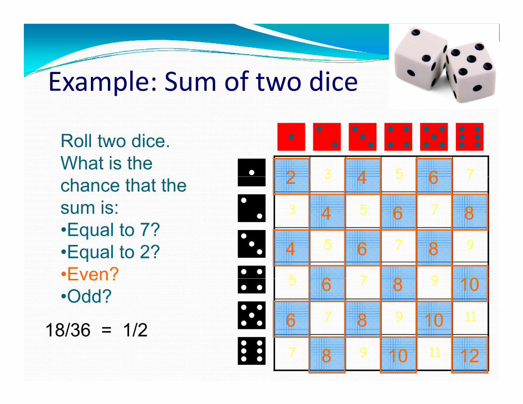
Roll two dice.What is the

2 642 3 4 5 6 7

3 4 5 6 7 8chance that the sum is:•Equal to 7?

2 64

4 864 5 6 7 8 9

5 6 7 8 9 10

•Equal to 7? •Equal to 2? •Even?

4 6 8

6 8 105 6 7 8 9 10

6 7 8 9 10 11

Even?•Odd? 6 8 10

6 8 1018/36 = 1/27 8 9 10 11 128 10 12

18/36 = 1/2

Example: Sum of two dice

2 3 4 5 6 7Roll two dice.What is the chance 2 642 3 4 5 6 7

3 4 5 6 7 8

What is the chance that the sum is:Equal to 7?

2 64

4 864 5 6 7 8 9

5 6 7 8 9 10

Equal to 7? Equal to 2? Even?

4 6 8

6 8 105 6 7 8 9 10

6 7 8 9 10 11

Odd? 6 8 10

6 8 1018/36 = 1/27 8 9 10 11 128 10 12

18/36 = 1/2

DefinitionDefinitionEvents A and B are disjoint (or mutually

l i ) if h hexclusive) if they cannot occur at the same time. (That is, disjoint events do not overlap.)

Venn Diagram for Events That Are Not Disjoint

Venn Diagram for Disjoint Events

Addition RuleAddition RuleProposition 1.1.1

P(AUB) = P(A) + P(B) – P(AB)where P(AB) denotes the probability that A andthe probability that A and B both occur at the same time as an outcome in atime as an outcome in a trial or procedure.

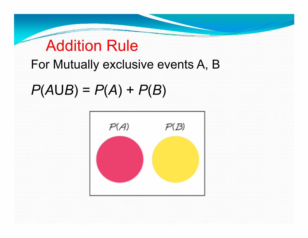
Addition RuleAddition RuleFor Mutually exclusive events A, B

P(AUB) = P(A) + P(B)

Example 1.1eSuppose the probabilities that the Dow‐Jones stock index increases today is .54, Jones stock index increases today is .54, that it increases tomorrow is .54, and that it increases both days is .28. What is the it increases both days is .28. What is the probability that it does not increase on either day?either day?

21

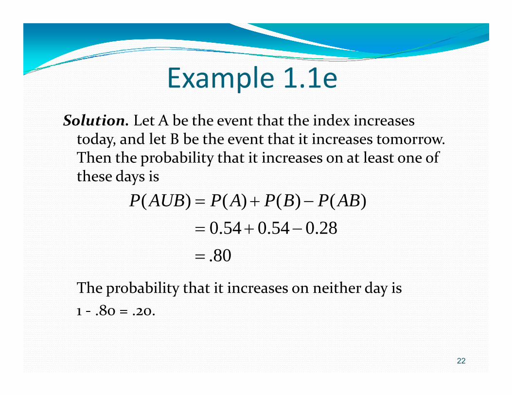
Example 1 1eExample 1.1eSolution  Let A be the event that the index increases Solution. Let A be the event that the index increases today, and let B be the event that it increases tomorrow. Then the probability that it increases on at least one of th  d  ithese days is

( ) ( ) ( ) ( )0 54 0 54 0 28

P AUB P A P B P AB 0.54 0.54 0.28.80

The probability that it increases on neither day is 1 ‐ .80 = .20.

22

DefinitionTh l t f t A d t d b AcThe complement of event A, denoted by Ac, consists of all outcomes in which the event A d tA does not occur.

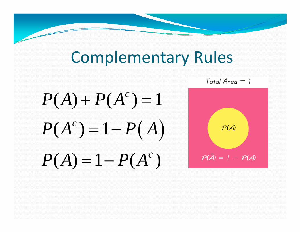
Complementary Rules

( ) ( ) 1cP A P A

( ) ( ) 1( ) 1c

P A P AP A P A

( ) 1

( ) 1 ( )c

P A P A

P A P A

( ) 1 ( )P A P A

S ti 1 2Section 1.2Conditional ProbabilityConditional Probability

25

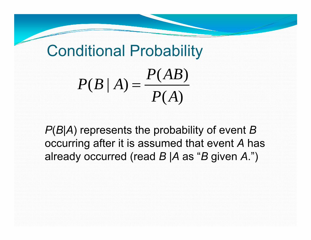
Conditional Probability( )P AB( )( | )( )

P ABP B AP A

P(B|A) represents the probability of event B( | ) p p yoccurring after it is assumed that event A has already occurred (read B |A as “B given A.”)

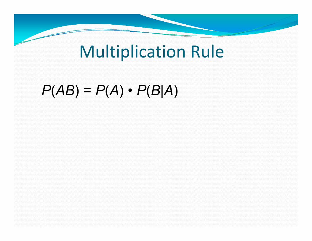
l l lMultiplication Rule

P(AB) = P(A) • P(B|A)

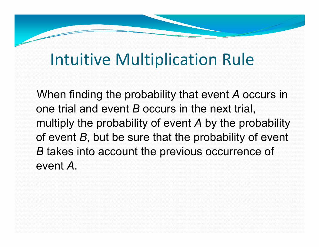
Intuitive Multiplication Rule

When finding the probability that event A occurs in one trial and event B occurs in the next trialone trial and event B occurs in the next trial, multiply the probability of event A by the probability of event B but be sure that the probability of eventof event B, but be sure that the probability of event B takes into account the previous occurrence of event A.

DefinitionsDefinitions Two events A and B are independent ifTwo events A and B are independent if

P(B|A) = P(B) A and B are independent if the occurrence of one A and B are independent if the occurrence of one

does not affect the probability of the occurrence of the other. In this case,

P(AB) = P(A) • P(B) If A and B are not independent they are said to beIf A and B are not independent, they are said to be

dependent.

Example 1.2cSuppose that, with probability .52, the closing price of a stock is at least as high closing price of a stock is at least as high as the close on the previous day, and that the results for successive days are the results for successive days are independent. Find the probability that the closing price goes down in each of the the closing price goes down in each of the next four days, but not on the following day.day.

30

Example 1 2cExample 1.2cSolution  Let A be the event that the closing Solution. Let Ai be the event that the closing price goes down on day i. Then, by independence, we havep ,

1 2 3 4 5 1 2 3 4 54

( ) ( ) ( ) ( ) ( ) ( )c cP A A A A A P A P A P A P A P A4(.48) (.52)

.0276

31

Multiplication rule for 3 Events

P(ABC) = P(AB)P(C|AB) = P(A) P(B|A) P(C|AB)P(ABC)   P(AB)P(C|AB)   P(A) P(B|A) P(C|AB)

M lti li ti l f E tMultiplication rule for n Events

P(A1 A2 … An)  =  P(A1 … An‐1)P(An|A1 … An‐1)

 P(A ) P(A |A ) P(A |A A )  P(A | A  A )= P(A1) P(A2|A1) P(A3|A1 A2)… P(An| A1 … An‐1)

A U f l T i kA Useful TrickTo find the probability of at least one ofTo find the probability of at least one of something, calculate the probability of none then subtract that result from 1none, then subtract that result from 1. That is,

P(at least one) = 1 – P(none).

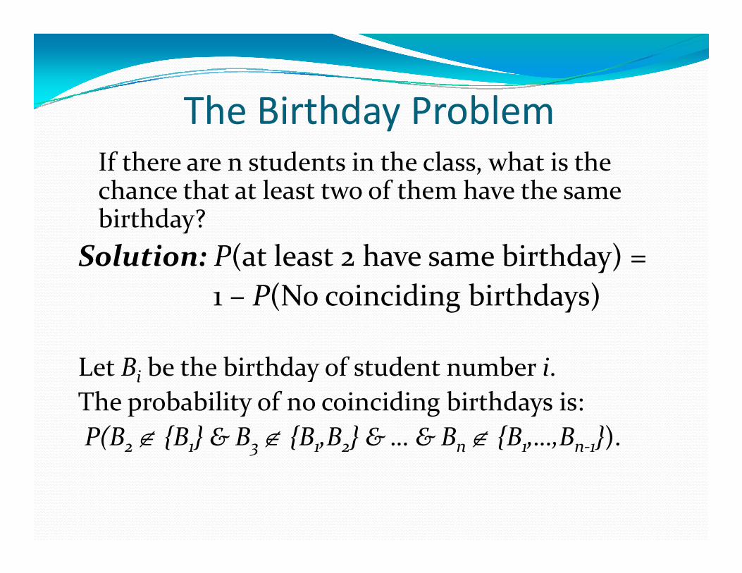
The Birthday ProblemThe Birthday ProblemIf there are n students in the class, what is the chance that at least two of them have the same birthday?

S l ti  P( t l t   h    bi thd )   Solution: P(at least 2 have same birthday) = 1 – P(No coinciding birthdays)

Let Bi be the birthday of student number i.Th   b bili   f    i idi  bi hd  iThe probability of no coinciding birthdays is:P(B2 {B1} & B3 {B1,B2} & … & Bn {B1,…,Bn‐1}).

The Birthda ProblemThe Birthday ProblemP(at least 2 have same birthday) P(at least 2 have same birthday) = 1 – P(No coinciding birthdays) 

1 2 n - 1= 1 - 1 ︵1 - ︶︵1 - ︶... ︵1 - ︶365 365 365

Q: How can we compute this for large n? A: Approximate!A: Approximate!

The Birthday ProblemThe Birthday Problem

log(P(No coinciding birthdays))log(P(No coinciding birthdays))

1 2 n - 1= log ︵ ︵1 - ︶ ︵1 - ︶... ︵1 - ︶ ︶

log ︵ ︵1 ︶ ︵1 ︶... ︵1 ︶ ︶365 365 3651 2 n - 1= log ︵1 - ︶+ log ︵1 - ︶+ + log ︵1 - ︶365 365 365

365 365 3651 2 n - 1≈ - - - -

365 365 365365 365 3651 1= - ︵ n ︵n - 1 ︶ ︶365 2

The Birthday Problem

n(n 1)

P(No coinciding birthdays) 2 365e

P(At least 2 have same birthday)

n(n 1)2 3651 e 1 e

Probabilities in the Birthday Problem

Shesh Besh BackgammonProbabilities in the Birthday Problem

1

0.70.80.9

0.40.50.6

0 10.20.3

00.1

2 22 42 62 82 100

n

Rule of AverageRule of Average Conditional Probabilities

If B1,…,Bn is a disjoint Partition of S, then

P(A)= P(AB1) + P(AB2) +…+ P(ABn)= P(A|B1)P(B1) + P(A|B2)P(B2)+…+P(A|Bn)P(Bn)

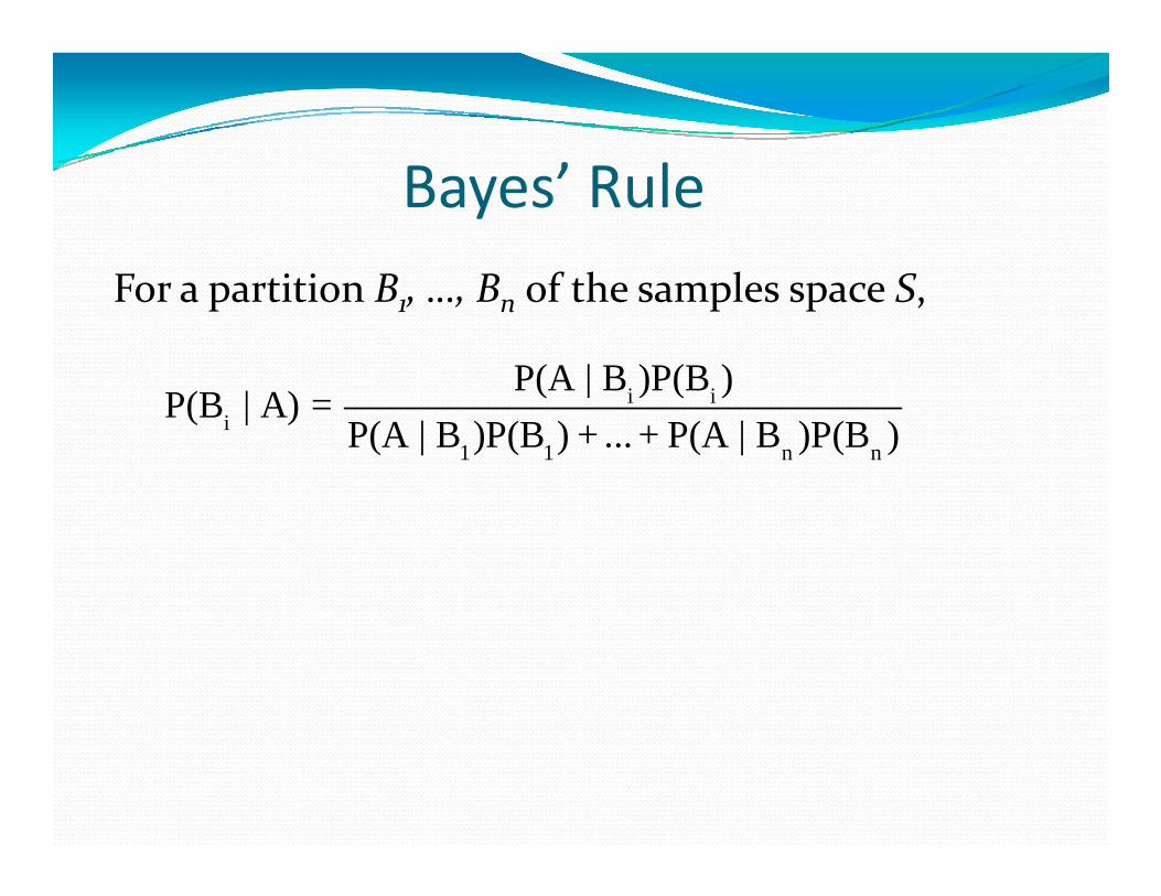
B ’ R lBayes’ Rule

F     titi B    B f th   l    SFor a partition B1, …, Bn of the samples space S,

i iP(A | B )P(B )( | A) i i

i1 1 n n

( | ) ( )P(B | A) =

P(A | B )P(B ) + ... + P(A | B )P(B )

M H ll blMonty Hall problem Here is classic problem. You are on the Monty Hall show.  You are presented with 3 doors (A, B, C), only one of which has something valuable to you y g ybehind it (the others are bogus). You do not know what is behind any of the doors.  You choose door A; Monty Hall opens door B and shows you that A; Monty Hall opens door B and shows you that there is nothing behind it.  Then he gives you the option of sticking with A or switching to C.  Do you stay or switch?  Does it matter?you stay or switch?  Does it matter?

Monty Hall problem The odds on Door A were still only 1 in 3 even after he opened another door  3 even after he opened another door. If you switch, you’ll win whenever your original choice was wrong  which original choice was wrong, which happens 2 out of 3 times.

Section 1 3Section 1.3Random Variables andRandom Variables and 

Expected Valuesp

44

DefinitionsDefinitions Random variable (RV) Random variable (RV)Numerical quantities whose values are determined by the outcome of the determined by the outcome of the experiment are known as random variables. Di t   d   i bl   Discrete random variable RV takes either a finite number of values or a countable number of values.

Probability distributionProbability distribution If X is a random variable whose possible If X is a random variable whose possible values are x1, x2, . . . , xn, then the set of probabilities  P{X = xj} ( j = 1, . . . , n) is called p { j} ( j , , )the probability distribution of the random variable.

b b l bProbability Distribution

( ) 0 for 1, 2,iP X x i n

( ) 1n

iP X x 1

ii

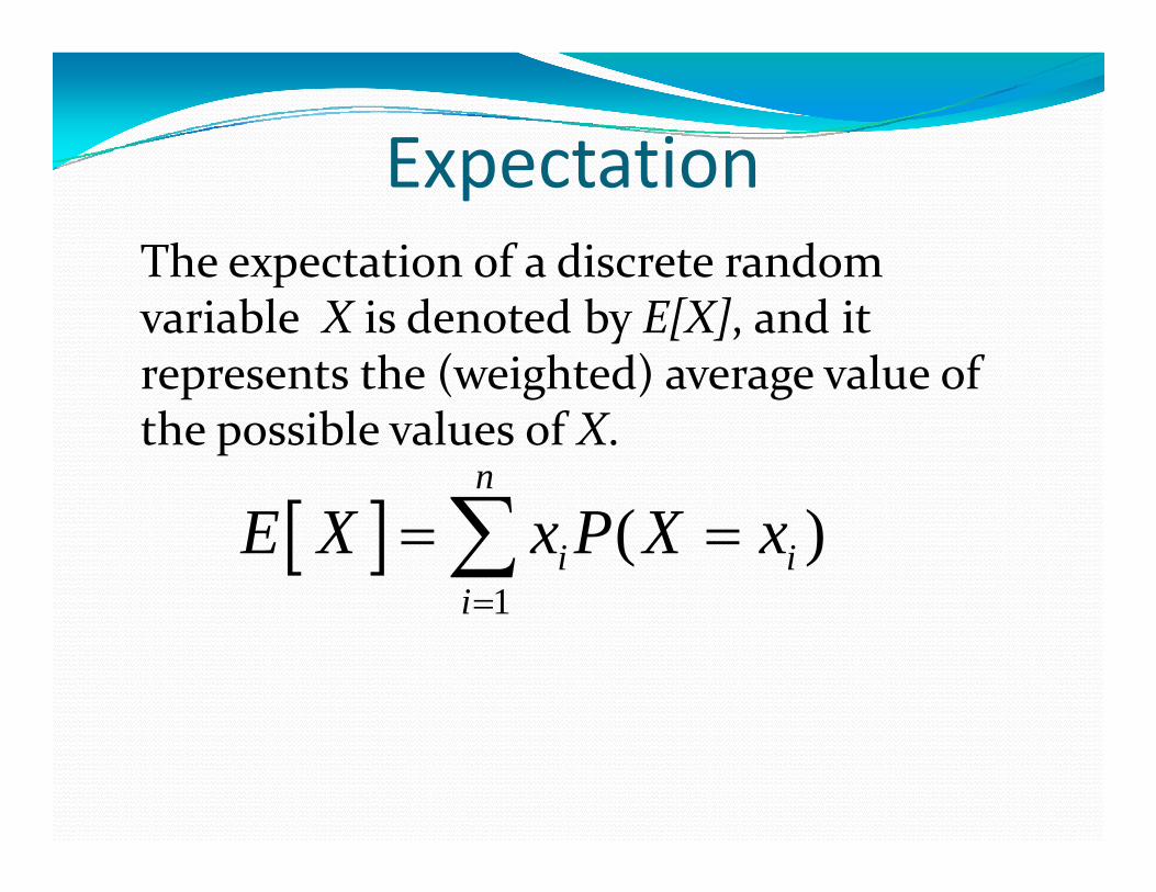
ExpectationExpectationThe expectation of a discrete random pvariable  X is denoted by E[X], and it represents the (weighted) average value of p ( g ) gthe possible values of X. 

n

1

( )i ii

E X x P X x

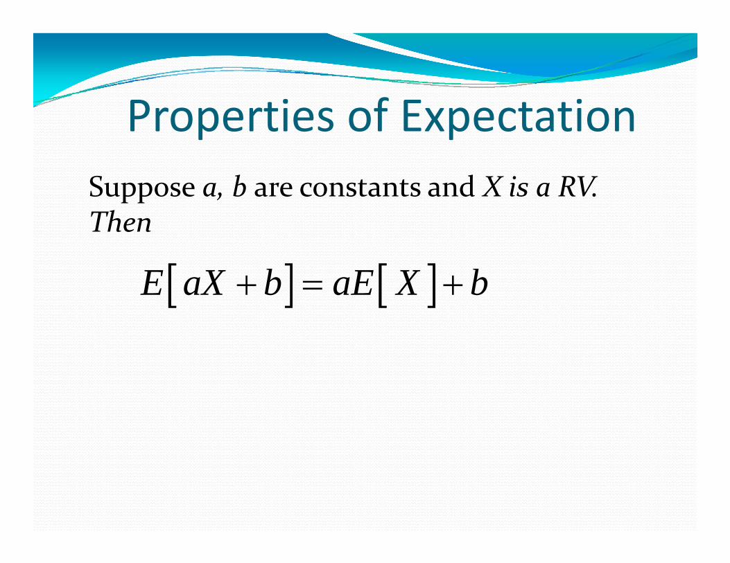
P ti f E t tiProperties of Expectationb dSuppose a, b are constants and X is a RV. 

Then

E aX b aE X b

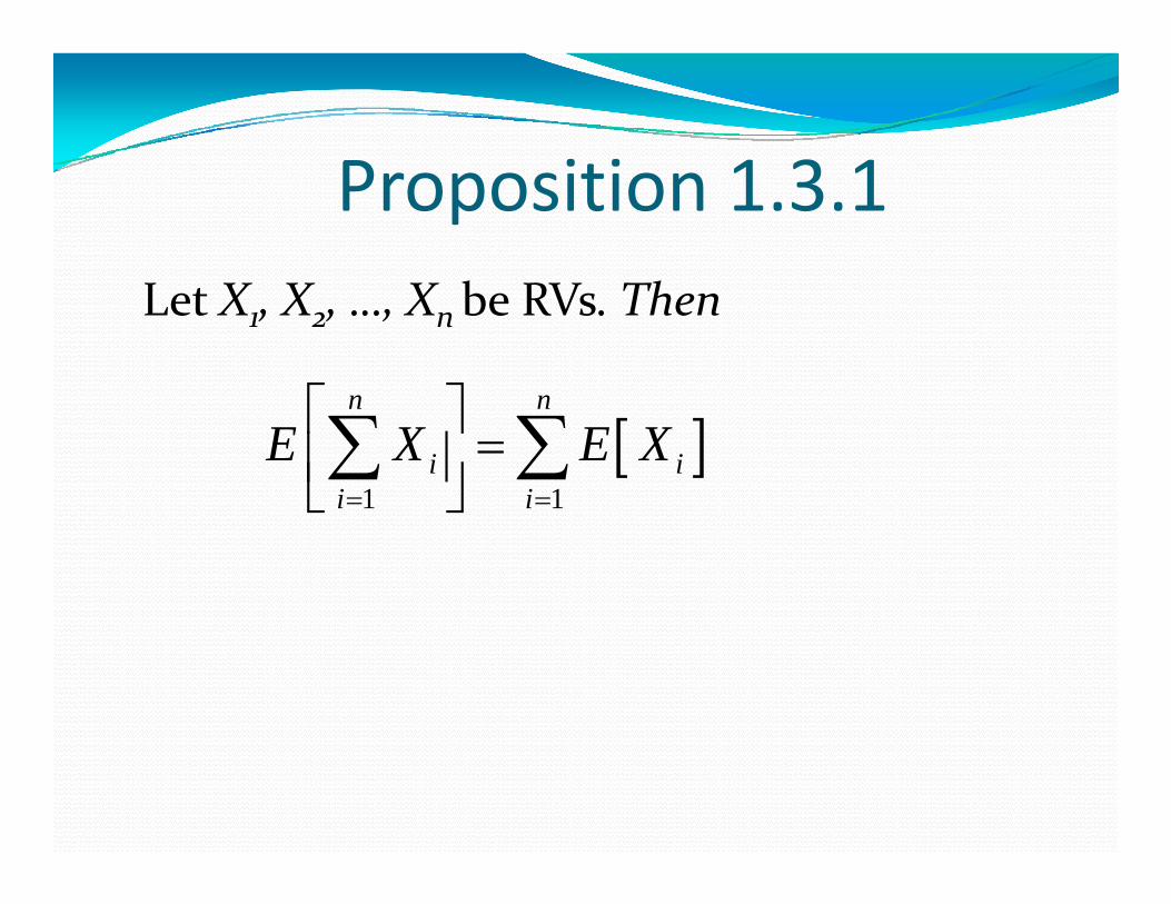
P iti 1 3 1Proposition 1.3.1b hLet X1, X2, …, Xnbe RVs. Then

1 1

n n

i ii i

E X E X

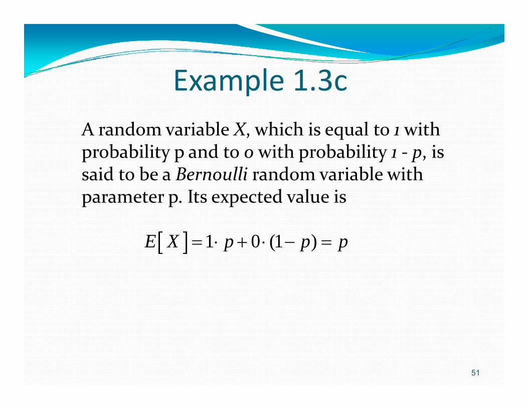
Example 1 3cExample 1.3cA random variable X  which is equal to 1 with A random variable X, which is equal to 1 with probability p and to 0 with probability 1 ‐ p, is said to be a Bernoulli random variable with said to be a Bernoulli random variable with parameter p. Its expected value is

1 0 (1 )E X p p p

51

Binomial Experiment

• The experiment has a fixed number of trials, n.

• The trials must be independent   • The trials must be independent.  

• Each trial must have all outcomes classified into t t i  ( l   f d t      two categories (commonly referred to as success and failure).

• The probability of a success remains the same, say p, in all trials.

Example 1 3dExample 1.3dLet X be the total number of successes that Let X be the total number of successes that occur in a binomial experiment. X is called a binomial random variable with parameters n binomial random variable with parameters n and p. Let Xj be the number of successes in trial j. Then Xj is a Bernoulli RV andj

1

n

jj

X X

1 1

n n

jj j

E X E X p np

1j

53

j j

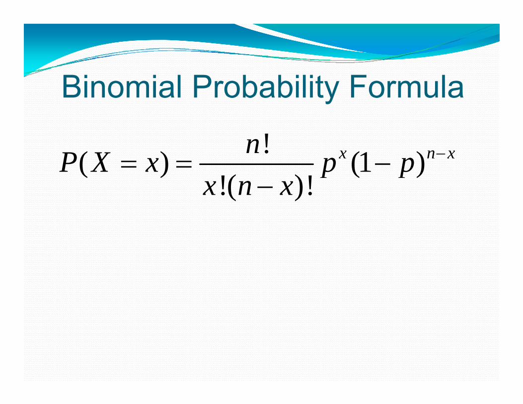
Binomial Probability Formula

!( ) (1 )!( )!

x n xnP X x p p ( ) ( )!( )!

p px n x

R ti l f th Bi i lRationale for the Binomial Probability Formulay

P(x) = • px • (1-p)n-xn ! (n x )!x!( ) p ( p)(n – x )!x!

The number ofThe number of outcomes with exactly x successes among n

trials

Rationale for the BinomialRationale for the Binomial Probability Formula

P(X=x) = • px • (1-p)n-xn ! (n – x )!x!

Number of outcomes with exactly

The probability of xsuccesses among noutcomes with exactly

x successes among ntrials

gtrials for any one particular order

I di tIndicatorsIndicators associate 0/1 valued randomIndicators associate 0/1 valued random variables to events.

Definition: The indicator of the event A, IAis the random variable that takes the value 1 for outcomes in A and the value 0 for outcomes in Ac.

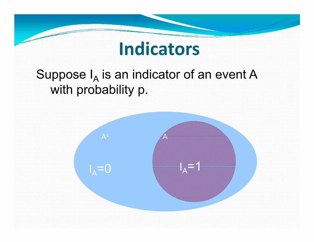
I di tIndicatorsSuppose I is an indicator of an event ASuppose IA is an indicator of an event A

with probability p.

Ac AAc A

I =1I =0 IA=1IA=0

E t ti f I di tExpectation of IndicatorsThen:Then:

E(IA)= 1*P(A) + 0*P(Ac) = P(A)E(IA) 1 P(A) + 0 P(A ) P(A)

P(Ac) P(A)P(Ac) P(A)

I =1I =0 IA=1IA=0

Expected Number of Events that OccurExpected Number of Events that Occur

Suppose there are n events A1, A2, …, An.Suppose there are n events A1, A2, …, An. Let X = I1 + I2 + … + In where Ii is the indicator of AiThen X counts the number of events that occur. By the addition rule:

E(X) = P(A1) + P(A2) + … P(An).( ) ( 1) ( 2) ( n)

Expectation of a Function of TwoExpectation of a Function of  Two Random Variables

E(g(X,Y))= { ll ( )} g(x,y)P(X=x, Y=y).E(g(X,Y))  {all (x,y)} g(x,y)P(X x, Y y).

Product of  Two Random VariablesE(XY) = {all (x,y)} xy P(X=x, Y=y)

E(XY) = x y xy P(X=x, Y=y)

Is E(XY) = E(X)E(Y)?

Product Rule for IndependentProduct Rule for Independent Random Variables

Theorem:  If X and Y are independent, ththen:

E(XY) =E(X) E(Y)

Product Rule for IndependentProduct Rule for Independent Random Variables

Proof: If X and Y are independent, P(X Y ) P(X )P(Y )P(X=x,Y=y)=P(X=x)P(Y=y)

thenE(XY)    P(X ) P(Y ) E(XY) = x y xy P(X=x) P(Y=y) 

= (xx P(X=x)) (y y P(Y=y)) ( ) ( )= E(X) E(Y)

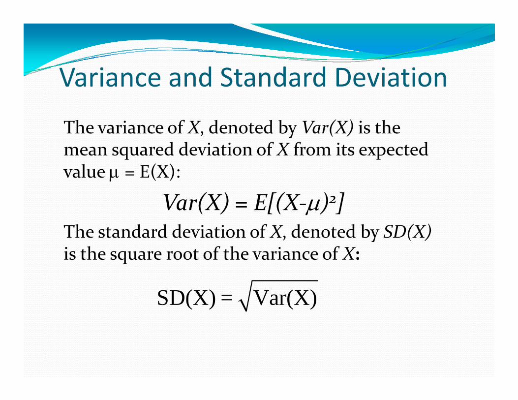
Variance and Standard DeviationVariance and Standard Deviation

Th   i   f X  d t d b  V (X) i  th  The variance of X, denoted by Var(X) is the mean squared deviation of X from its expected value  = E(X):value  = E(X):

Var(X) = E[(X‐)2]Th   d d d i i   f X  d d b  SD(X) The standard deviation of X, denoted by SD(X) is the square root of the variance of X:

SD(X) = Var(X)

Computational Formula forComputational Formula for Variance

2 2Var(X) = E(X ) - E(X)Claim:

Proof:

E[ (X-)2] = E[X2 – 2 X + 2]

E[ (X-)2] = E[X2] – 2 E[X] + 2E[ (X ) ] E[X ] 2 E[X] +

E[ (X-)2] = E[X2] – 22+ 2

E[ (X-)2] = E[X2] – E[X]2

Properties of Variance and SDTheorem:

Var(X) ≥ 0 andVar(X) = 0 iff P[X=] = 1.

Proof: Var(X) = (x-)2 P(X=x)Proof: Var(X) (x ) P(X x)

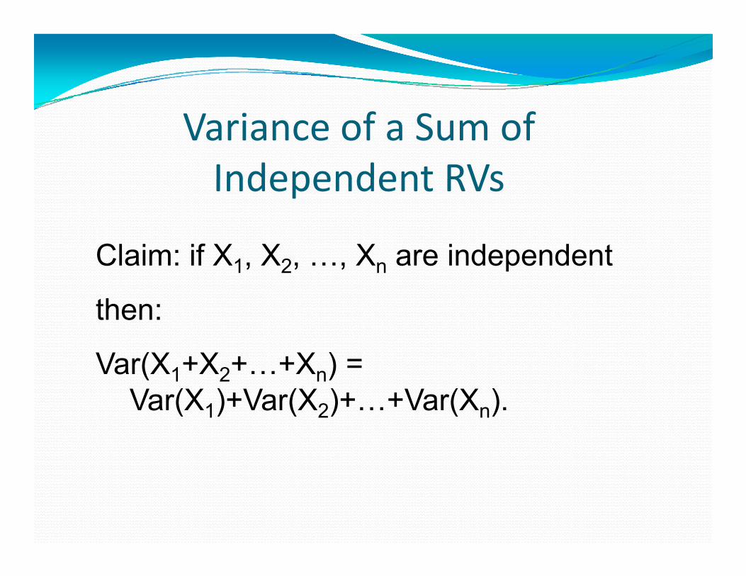
Variance of a Sum of Independent RVsIndependent RVs

Claim: if X X X are independentClaim: if X1, X2, …, Xn are independent

then:

Var(X1+X2+…+Xn) = Var(X )+Var(X )+ +Var(X )Var(X1)+Var(X2)+…+Var(Xn).

Variance of a Sum ofVariance of a Sum of Independent RVsp

Proof: Suffices to prove for 2 random variables. p

2 2

2 2

E X+Y – E X+Y = E X-E X + Y–E Y

2 2= E X-E X + 2 E X-E X Y-E Y + E Y–E Y

= Var X +Var Y + 2E X-E X E Y-E Y

= Var X +Var Y + 0

Example 1 3fExample 1.3fFor Bernoulli random variable X  For Bernoulli random variable X, 

2( [ ])Var X E X E X 2

( [ ])

( )

Var X E X E X

E X p

2 2

( )

(1 ) (0 ) (1 )

p

p p p p

(1 ) [(1 ) ]

(1 )p p p p

70

(1 )p p

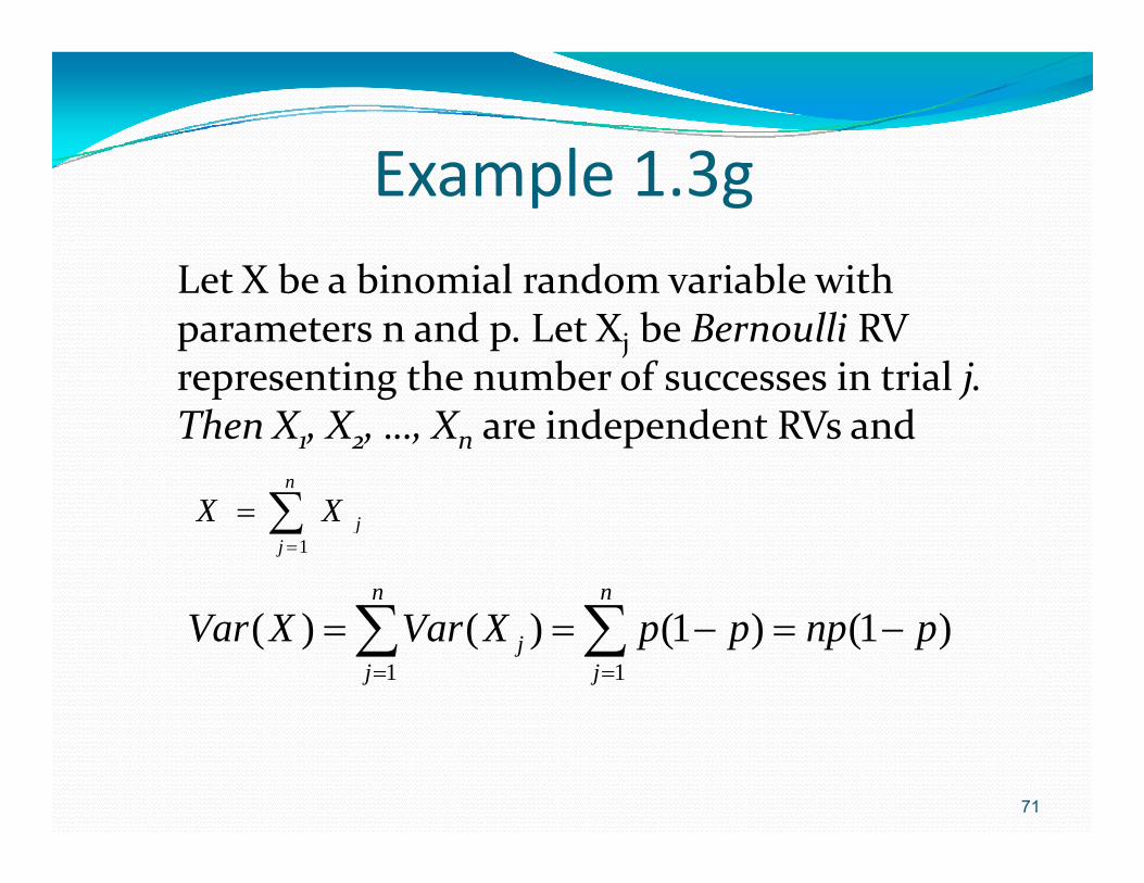
Example 1 3gExample 1.3gLet X be a binomial random variable with Let X be a binomial random variable with parameters n and p. Let Xj be Bernoulli RV representing the number of successes in trial j. representing the number of successes in trial j. Then X1, X2, …, Xn are independent RVs and

n

n n

1j

j

X X

1 1( ) ( ) (1 ) (1 )j

j jVar X Var X p p np p

71

Variance and Mean underVariance and Mean under scaling and shiftsg

Theorem:

SD(aX + b) = |a| SD(X)

Variance and Mean under scalingVariance and Mean under scaling and shifts

Proof:

Var[aX+b] = E[(aX+b – a –b)2]

= E[a2(X-)2 ]

= a2 E[(X-)2]= a E[(X-) ]

a2 Var[X]

Variance and Mean forVariance and Mean for Standardized RV

Corollary: If a random variable X has yE(X) = and SD(X) = > 0,

Then Z=(X-)/ has E(Z) =0 and SD(Z)=1

Section 1.4Covariance and CorrelationCovariance and Correlation

75

Definition of CovarianceDefinition of Covariance

( , ) ( [ ])( [ ])Cov X Y E X E x Y E Y

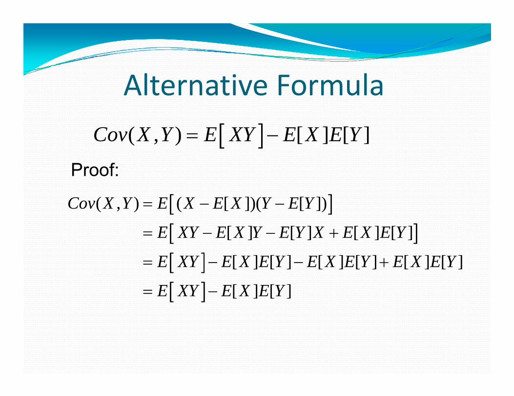
l lAlternative Formula

( , ) [ ] [ ]Cov X Y E XY E X E Y

Proof:Proof:

( , ) ( [ ])( [ ])Cov X Y E X E X Y E Y

[ ] [ ] [ ] [ ]

[ ] [ ] [ ] [ ] [ ] [ ]

E XY E X Y E Y X E X E Y

E XY E X E Y E X E Y E X E Y

[ ] [ ]E XY E X E Y

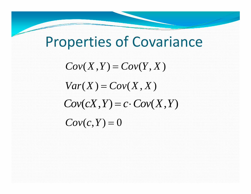
fProperties of Covariance

( , ) ( , )Cov X Y Cov Y X

( ) ( )Var X Cov X X( ) ( , )Var X Cov X X

( , ) ( , )Cov cX Y c Cov X Y ( ) ( )( , ) 0Cov c Y

Linear Properties of Covariance( ) ( ) ( )Cov X X Y Cov X Y Cov X Y 1 2 1, 2( , ) ( ) ( , )Cov X X Y Cov X Y Cov X Y

Proof:

1 2 1 2 1 2

1 2 12 2

( , ) ( ) [ ] [ ]

( [ ] [ ]) [ ]

Cov X X Y E X X Y E X X E Y

E X Y X Y E X E X E Y

1 2 12 2

1 1 2 2

( [ ] [ ]) [ ]

[ ] [ ] [ ] [ ]( ) ( )

E X Y E X E Y E X Y E X E YCov X Y Cov X Y

1 2( , ) ( , )Cov X Y Cov X Y

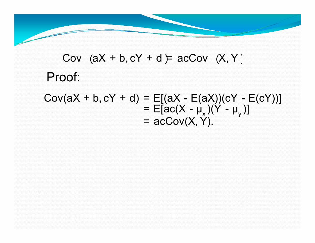
Cov ︵aX + b, cY + d ︶ = acCov ︵X, Y ︶

Proof:Cov(aX + b, cY + d) = E[(aX - E(aX))(cY - E(cY))]

E[ (X )(Y )]

Proof:

x y = E[ac(X - μ )(Y - μ )] = acCov(X, Y).

V i d C i

Variance and Covariance

n m n m

i j i ji 1 j 1 i 1 j 1

X YCov , = Cov(X , Y )

n n nX Var X( )Var = Cov(X X )

i i i ji 1 i 1 i 1 j i

X Var X( )Var Cov(X , X )

C l iCorrelation

X ‐ E(X) Y ‐ E(Y)ρ(X, Y) = Corr(X, Y) = ESD(X) SD(Y) SD(X) SD(Y)

C l iCorrelationU i  th  li it   f E t ti     t:

ρ(aX + b, cY + d) = ρ(X, Y)

Using the linearity of Expectation we get:

ρ(aX + b, cY + d) ρ(X, Y)

Correlation is invariant of scale change!Correlation is invariant of scale change!

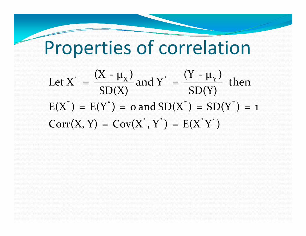
P ti f l tiProperties of correlation(X μ ) (Y μ )

* *X Y

* * * *

(X ‐ μ ) (Y ‐ μ )Let X =  and Y = then

SD(X) SD(Y)E(X ) E(Y )   d SD(X ) SD(Y )

* * * *

E(X ) = E(Y ) = 0 and SD(X ) = SD(Y ) = 1Corr(X, Y) = Cov(X , Y ) = E(X Y )

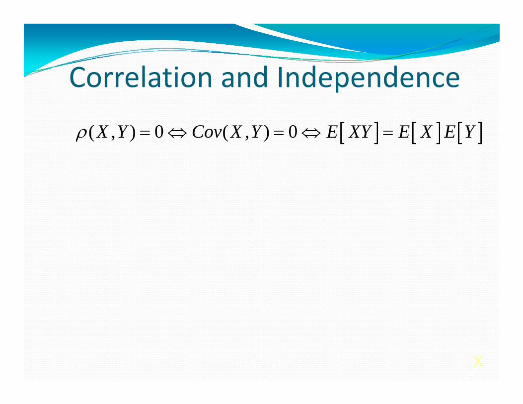
Correlation and IndependenceCorrelation and Independence

( ) 0 ( ) 0X Y C X Y E XY E X E Y ( , ) 0 ( , ) 0X Y Cov X Y E XY E X E Y

X

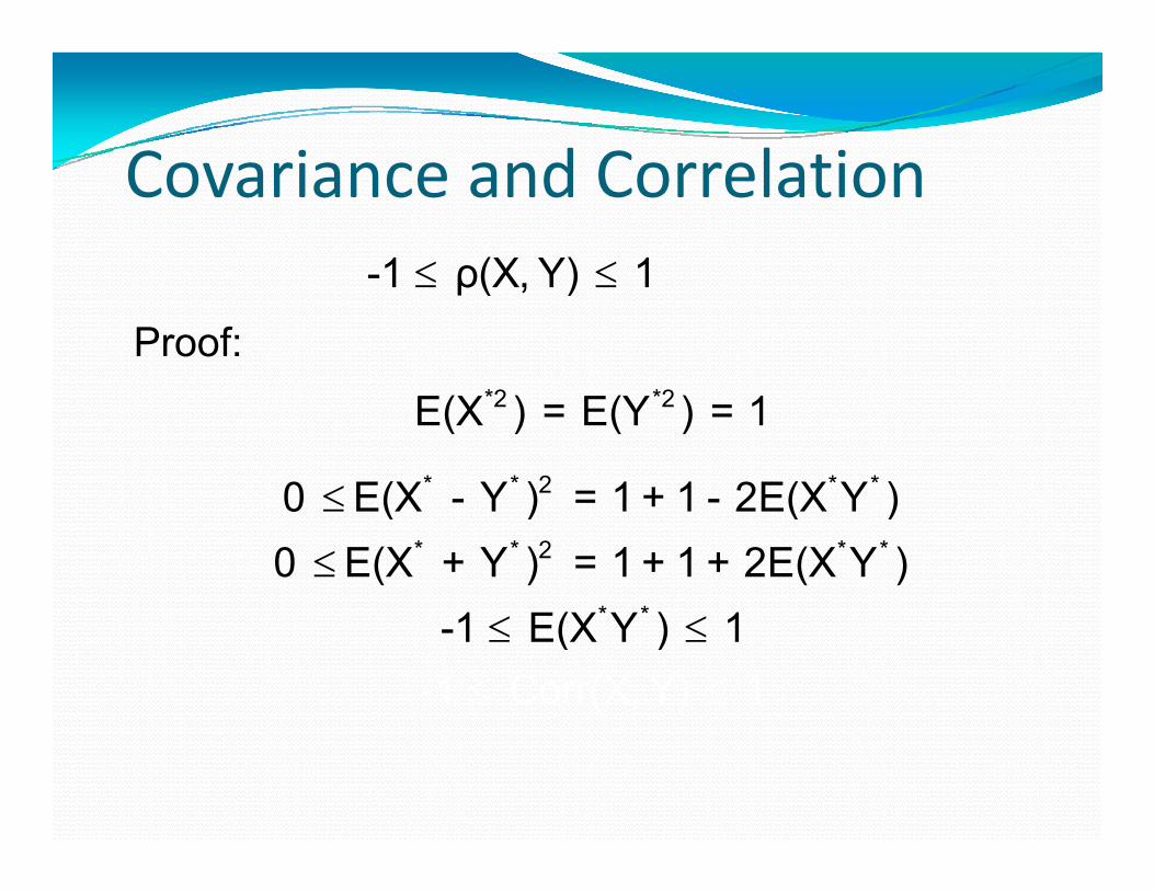
Covariance and CorrelationCovariance and Correlation -1 ρ(X Y) 1

*2 *2

-1 ρ(X, Y) 1

Proof:

*2 *2

* * 2 * *

E(X ) = E(Y ) = 1

0 E(X - Y ) = 1 + 1 - 2E(X Y )

* * 2 * *

* *

0 E(X - Y ) = 1 + 1 - 2E(X Y )0 E(X + Y ) = 1 + 1 + 2E(X Y )

1 E(X Y ) 1 -1 E(X Y )

-1 Corr(X, Y)11

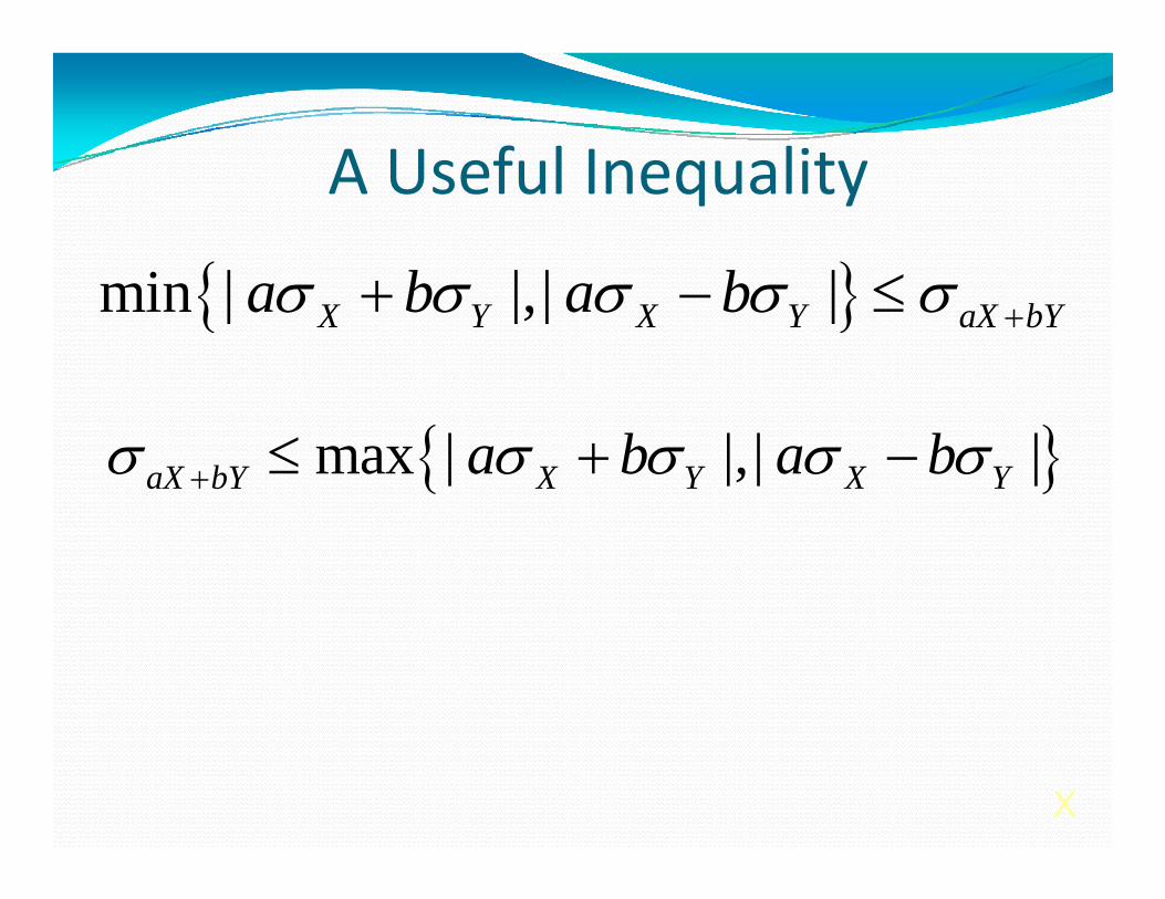
A Useful InequalityA Useful Inequality

i | | | |b b min | |,| |X Y X Y aX bYa b a b

max | |,| |aX bY X Y X Ya b a b

X

min | |,| | max | |,| |X Y X Y aX bY X Y X Ya b a b a b a b

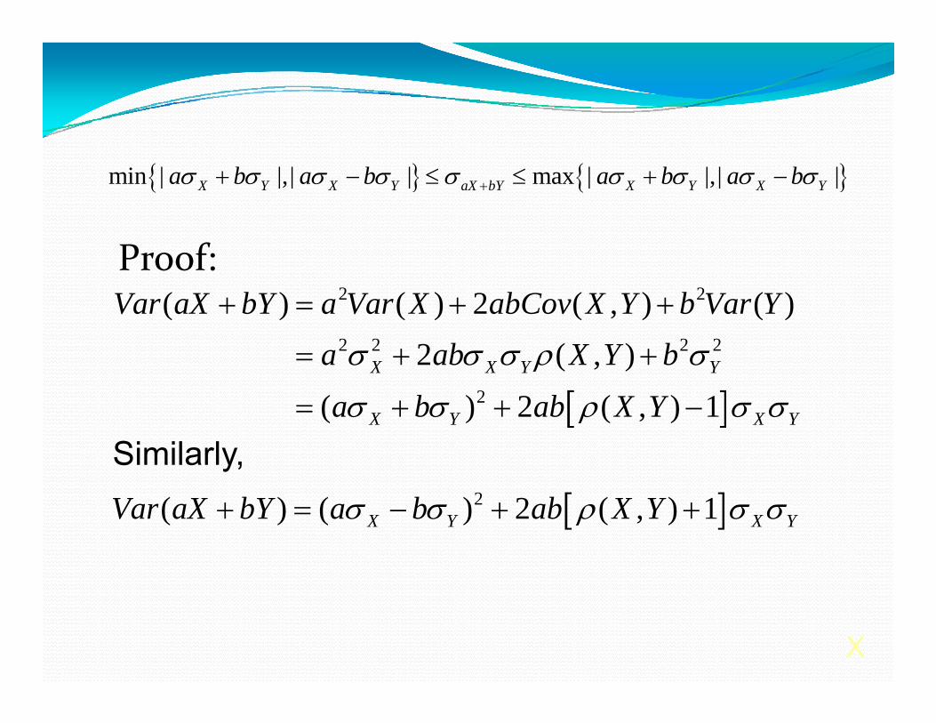
Proof:2 2( ) ( ) 2 ( , ) ( )Var aX bY a Var X abCov X Y b Var Y

2 2 2 2

2

( ) ( ) ( , ) ( )2 ( , )

( ) 2 ( ) 1X X Y Ya ab X Y b

a b ab X Y

( ) 2 ( , ) 1X Y X Ya b ab X Y Similarly,

2( ) ( ) 2 ( ) 1V X bY b b X Y 2( ) ( ) 2 ( , ) 1X Y X YVar aX bY a b ab X Y

X

Case 1: ab > 0 2 2( ) ( ) 2 ( , ) 1 ( )X Y X Y X YVar aX bY a b ab X Y a b

and 2 2( ) ( ) 2 ( ) 1 ( )V X bY b b X Y b

( ) ( ) ( , ) ( )X Y X Y X Y

2 2( ) ( ) 2 ( , ) 1 ( )X Y X Y X YVar aX bY a b ab X Y a b

Therefore2 2( ) ( ) ( )X Y X Ya b Var aX bY a b

i.e.i.e.

| | | |X Y aX bY X Ya b a b

X

Case 2: ab < 0

By a similar argument as case 1By a similar argument as case 1,

| | | |X Y aX bY X Ya b a b | | | |X Y aX bY X Y

Hence, in either case, we have

min | |,| |X Y X Y aX bYa b a b

max | |,| |aX bY X Y X Ya b a b

X

A Useful InequalityA Useful InequalitySuppose X and Y represent the returns pp pof two investments in a portfolio consists only of these two investments. yThen aX+bY is the return of the portfolio and a+b = 1. p

If a and b are both non‐negative (no shorting is allowed)  then the shorting is allowed), then the inequality becomes 

| |X Y X bY X Ya b a b

X

| | X Y aX bY X Ya b a b

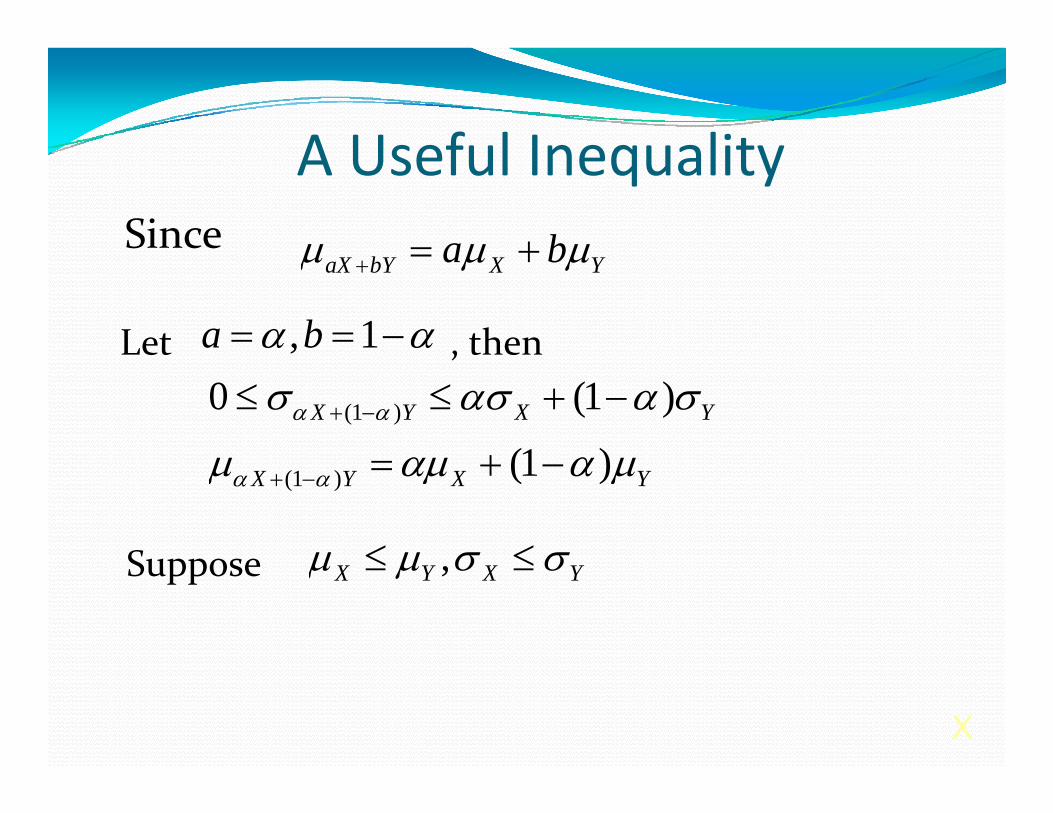
A Useful InequalityA Useful InequalitySince a b aX bY X Ya b

, 1a b Let                              , then

(1 )0 (1 )

(1 )X Y X Y

,

(1 ) (1 )X Y X Y

Suppose ,X Y X Y Suppose

X

A Useful InequalityA Useful Inequality

As α decreases from 1 to 0  the expected As α decreases from 1 to 0, the expected return increases from E(X) to E(Y). The risk of the portfolio (in terms of SD) does not of the portfolio (in terms of SD) does not necessarily in tandem with the expected. By adding a high‐risk investment with high expected returns to low‐risk investment with low expected returns, it may be 

ibl  t  i   t   d d  possible to increase return and decrease risk simultaneously!

X

Chapter 2Chapter 2Normal Random Variables

2.1 Continuous Random Variables

2.2 Normal Random Variables

2.3 Properties of Normal Random Variablesp

2.4 The Central Limit Theorem

2.5 Exercises

S ti 2 1Section 2.1Continuous RandomContinuous Random 

VariablesVariables

95

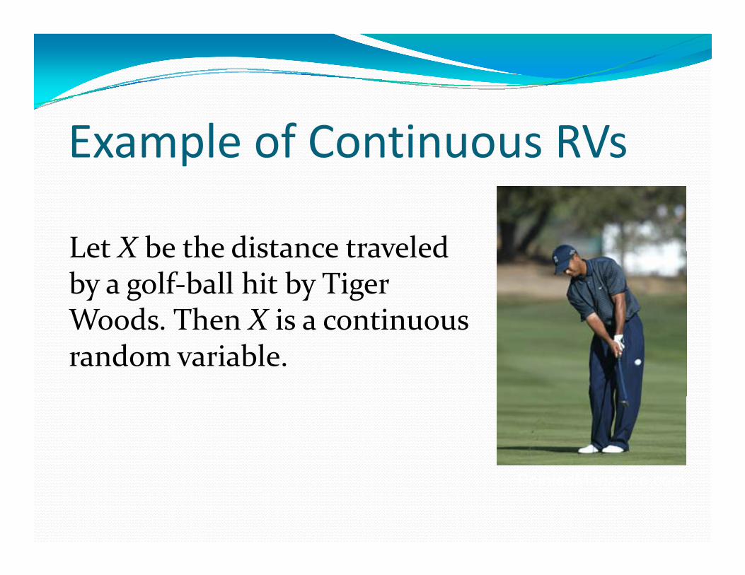
Example of Continuous RVs

Let X be the distance traveled Let X be the distance traveled by a golf‐ball hit by Tiger Woods  Then X is a continuous Woods. Then X is a continuous random variable.

PointedMagazine.com

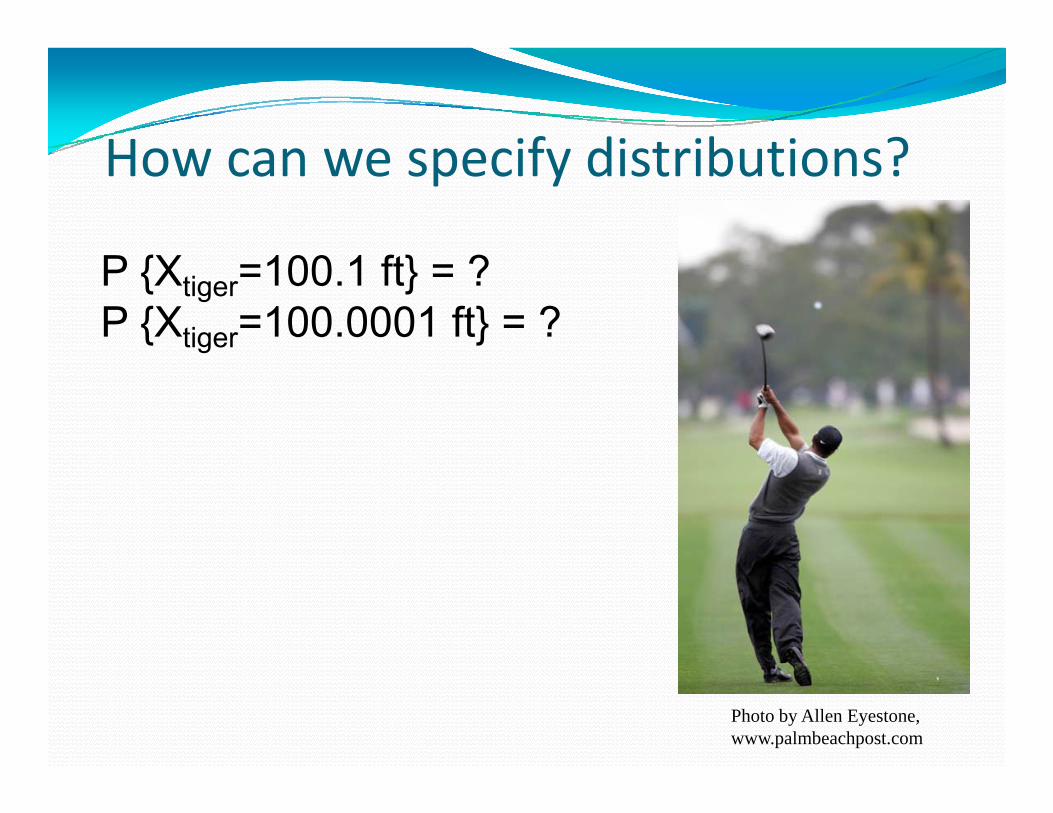
How can we specify distributions?How can we specify distributions?

P {Xtiger=100.1 ft} = ? P {Xtiger=100.0001 ft} = ?

Photo by Allen Eyestone, www.palmbeachpost.com

C ti Di t ib tiContinuous Distribution• A continuous distribution is determined by a y

probability density f(x). • Probabilities are defined by areas under the

f f( )graph of f(x)≥0.• The total area under the curve must equal 1.

b

P(a X b) f x dxa

C i Di ib iContinuous Distributions

Example: For the golf hit we will have:100.1

99 9

(99.9 100.1) ( )tigerP X f x dx

where ftiger is the probability density of X.

99.9

tiger p y y

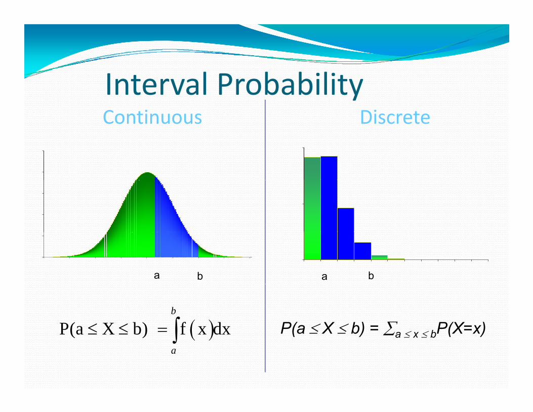
I t l P b bilitInterval ProbabilityContinuous  Discrete

a b a b

P(a X b) = a x bP(X=x) P(a X b) f x dxb

( ) a x b ( ) ( )a

ExpectationspContinuous Discrete

•Expectation of a function g(X):

( ) ( ) ( )E g x g x f x dx

all x

( ) ( ) ( )E g X g x P X x

•Variance and SD:

2( ) ( ( ))

( ) ( )

Var X E X E X

SD X Var X

( ) ( )

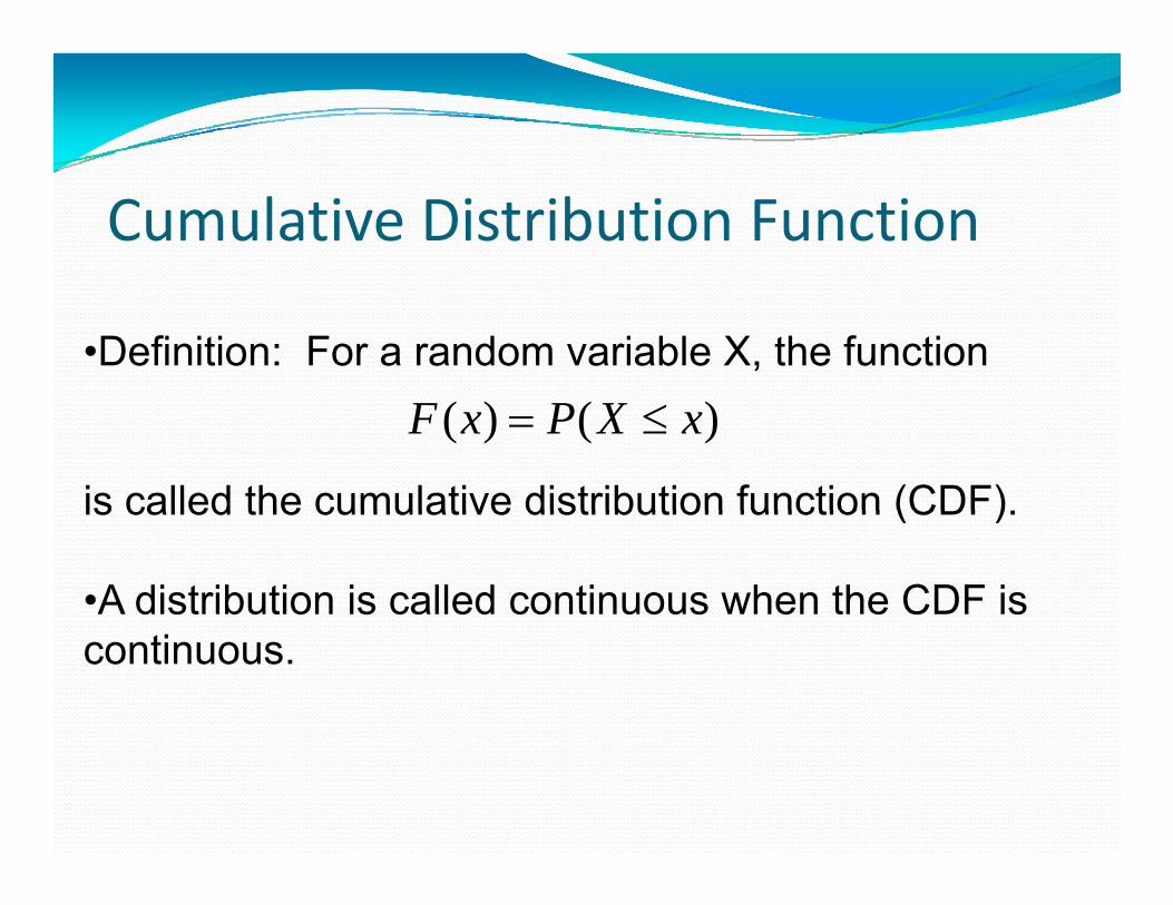
Cumulative Distribution Function

•Definition: For a random variable X, the function

is called the cumulative distribution function (CDF)

( ) ( )F x P X x

is called the cumulative distribution function (CDF).

•A distribution is called continuous when the CDF is continuous.

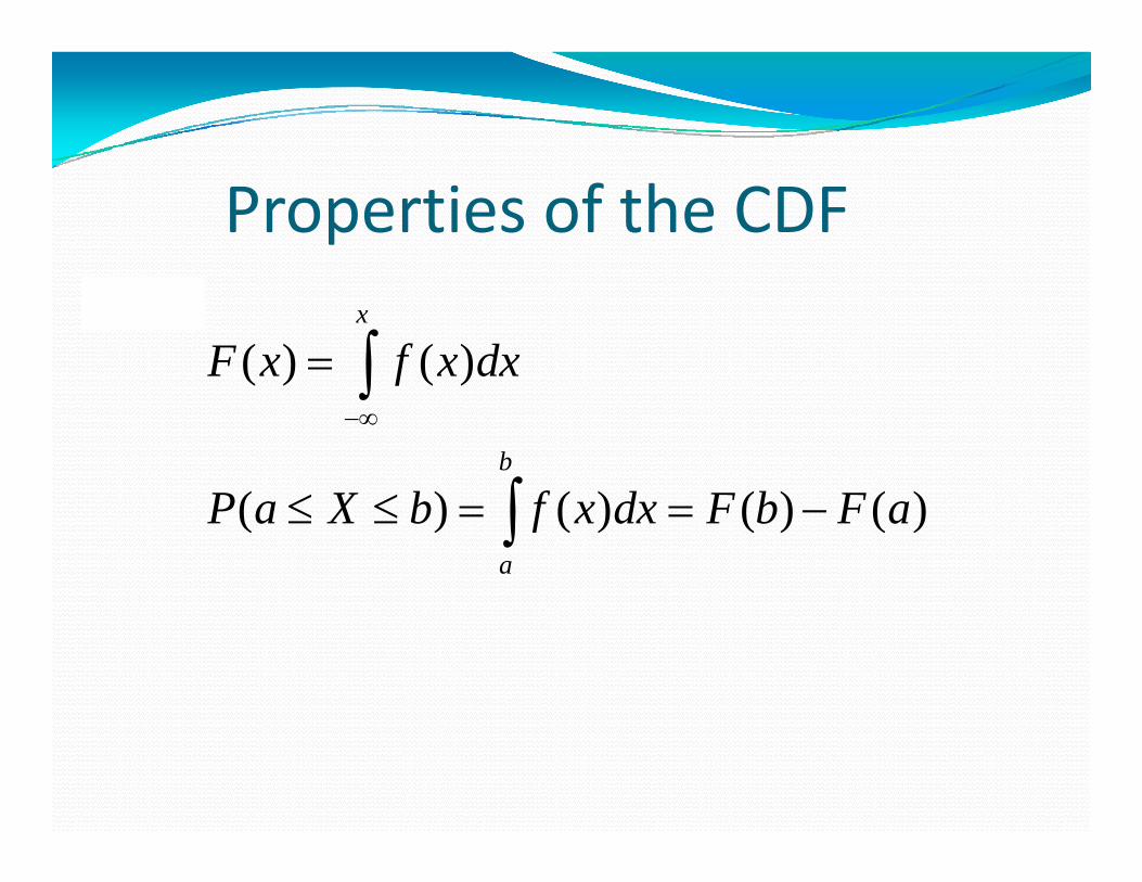
Properties of the CDF

( ) ( )x

F x f x dx ( ) ( )

( ) ( ) ( ) ( )b

f

P X b f d F b F

( ) ( ) ( ) ( )a

P a X b f x dx F b F a

U if Di t ib tiUniform DistributionA continuous random variable has a uniform distribution if its values spread evenly over the range of probabilities.  The graph of a uniform di ib i   l  i     l   hdistribution results in a rectangular shape.

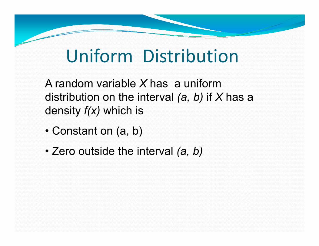
Uniform  DistributionA random variable X has a uniform distribution on the interval (a, b) if X has a d it f( ) hi h idensity f(x) which is

• Constant on (a, b)

• Zero outside the interval (a, b)

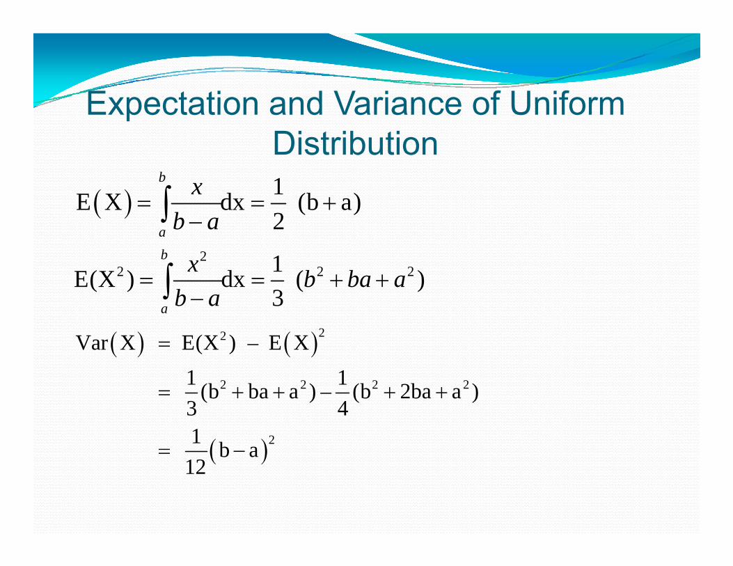
Expectation and Variance of UniformExpectation and Variance of Uniform Distribution

b

1E X dx (b a)2

b

a

xb a

22 2 21E(X ) dx ( )

3

b

a

x b ba ab a

22

2 2 2 2

Var X E(X ) – E X1 1(b ba a ) (b 2ba a )

2

(b ba a ) – (b 2ba a ) 3 41 b a

12

12

Section 2.2N l R d V i blNormal Random Variables

107

The Standard Normal Distribution

Definition: A continuous random variable Z has a standard normal distribution if Z has a probability density of the following form:

2(z)

-21

f(z)= (z)= e , (- <z< )2

∞ ∞2π

DefinitionThe standard normal distribution is a probability distribution with mean equal to 0probability distribution with mean equal to 0 and standard deviation equal to 1, and the total area under its density curve is equal to 1.y q

2(z)-21f(z) e ( <z< )

2f(z) e , (- <z< )

2

Standard Normal Integrals

∞ 2(x)‐

21 e dx = 12π∞‐ 2π

∞ 2(x)‐

21E(Z) e d 0∞

2

‐

E(Z) = x e dx = 02π

2(x)‐2 21Var(Z) = x e dx = 1

2π

∞

‐ 2π∞

Standard Normal CumulativeStandard Normal

Standard Normal Cumulative Distribution Function:

2z (x)‐

21Φ(z) = e dx

P(  Z b)   (b)  ( )

‐

( )2π

P(a Z b) = (b) ‐ (a)

Th l f t b l t d iThe value of are tabulated in the standard normal table 2.1

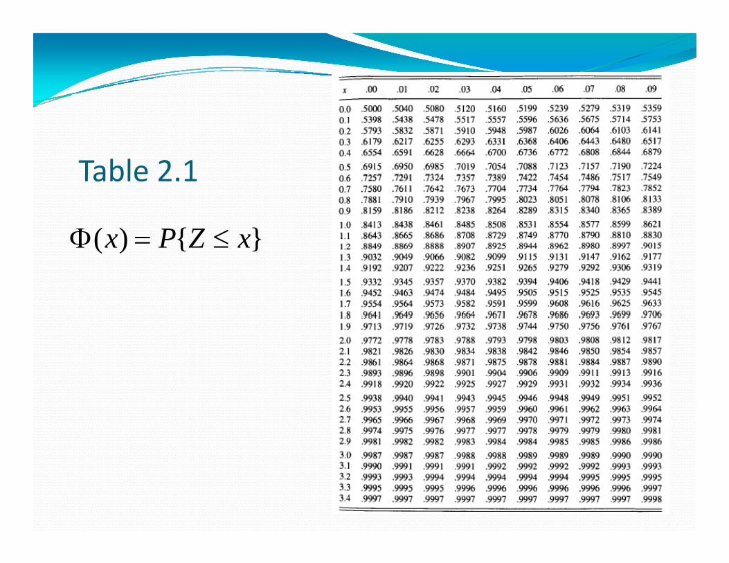
Table 2 1Table 2.1

( ) { }x P Z x ( ) { }x P Z x

Approximation to Φ(x)When greater accuracy than that provided by Table 2.1 is needed, the following y gapproximation to Φ(x), accurate to six decimal places, can be used: For x > 0,p

2 2 3 4 51 2 3 4 5

1( ) 1 ( )2

xx e a y a y a y a y a y

Where

2

Approximation to Φ(x)11

1 .2316419y

x

1 .319381530356563782

aa

2

3

.3565637821.781477937

aa

3

4 1.821255978a

5 1.330274429a

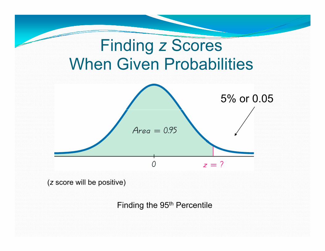
Finding z ScoresFinding z Scores When Given Probabilities

5% or 0.05

(z score will be positive)

Finding the 95th PercentileFinding the 95th Percentile

Finding z ScoresFinding z Scores When Given Probabilities - cont

5% or 0.05

Finding the 95th Percentile

1.645(z score will be positive)

Finding the 95th Percentile

Finding z ScoresFinding z Scores When Given Probabilities - cont

Fi di th B tt 2 5% d U 2 5%

(One z score will be negative and the other positive)

Finding the Bottom 2.5% and Upper 2.5%

Finding z ScoresFinding z Scores When Given Probabilities - cont

Fi di th B tt 2 5% d U 2 5%

(One z score will be negative and the other positive)

Finding the Bottom 2.5% and Upper 2.5%

S ti 2 3Section 2.3Properties of NormalProperties of Normal Random VariablesRandom Variables

119

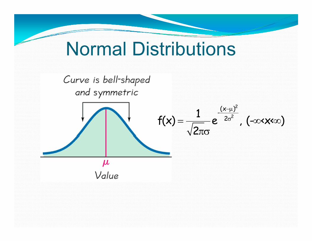
N l Di t ib tiNormal Distributions

2

2

2(x )-

21f(x) e , (- <x< )2

The Normal DistributionD fi iti If Z h t d d lDefinition: If Z has a standard normal distribution and and are constants th X Z + h l di t ib tithen X = Z + has a normal distribution with mean μ and standard deviation σ.

The Normal Distribution

E(X) = E( Z + ) = E(Z) + =

Var(X) = Var( Z + ) = E(Z) =

Normal( 2)Normal(,2)  25, 3.54.12

50, 508

.10

125, 7.91 250 11 2

.06

.08

250, 11.2

.02

.04

.00

0 50 100 150 200 250 300

Converting to a StandardConverting  to a Standard Normal DistributionNormal Distribution

P(c X d) = P(c  Z +  d) ( ) ( )= P((c‐ Z  (d‐ )= (c‐) ‐ (d‐)( ) ( )

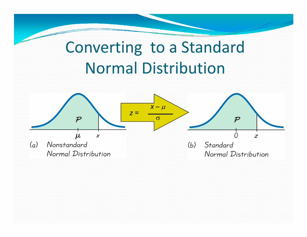
C ti t St d dConverting  to a Standard Normal Distribution

x –

z =

Example 2 3aExample 2.3aIQ examination scores for sixth‐graders are IQ examination scores for sixth graders are normally distributed with mean value 100 and standard deviation 14.2. What is the probability that a randomly chosen sixth‐grader has an IQ score greater than 130?

126

Example 2 3aExample 2.3aSolution. Let X be the score of a randomly chosen Solution. Let X be the score of a randomly chosen sixth‐grader. Then

100 130 100X 100 130 100{ 130}14.2 14.2

XP X P

{ 2.113}1 (2 113)P Z

1 (2.113).017

127

Example 2 3dExample 2.3dStarting at some fixed time, let S(n) denote the Starting at some fixed time, let S(n) denote the price of a certain security at the end of n additional weeks, n ≥ 1. A popular model for the evolution of these prices assumes that the price ratios S(n)/S(n ‐ 1) for n ≥ 1 are independent and id ti ll  di t ib t d (i i d ) l l identically distributed (i.i.d.) lognormal random variables. Assuming this model, with lognormal parameters μ =  0165 and σ =  0730  lognormal parameters μ = .0165 and σ = .0730, what is the probability that

128

Example 2 3dExample 2.3d(a) the price of the security increases over each of (a) the price of the security increases over each of the next two weeks;

(b) the price at the end of two weeks is higher ( ) p gthan it is today?

Solution. Let Z be a standard normal random variable. It is easy to see that

129

Example 2 3dExample 2.3d(a) (a)

(1) (1)1 ln 0(0) (0)

S SP PS S

( ) ( )

0 .01650730

P Z

.0730.2260P Z

.2260P Z

130

.5894

Example 2 3dExample 2.3dTherefore, the probability that the price is up Therefore, the probability that the price is up after one week is .5894. Since the successive price ratios are independent, by the multiplication rule, the probability that the price increases over each of the next two weeks iis

.58942 = .3474

131

Example 2 3dExample 2.3d(b)(b)

(2) (2) (1)1 1S S SP P

1 1(0) (1) (0)

(1) (1)

P PS S S

S S

(1) (1)ln ln 0(0) (0)

S SPS S

0 2(.0165)

0730 2P Z

132

.0730 2

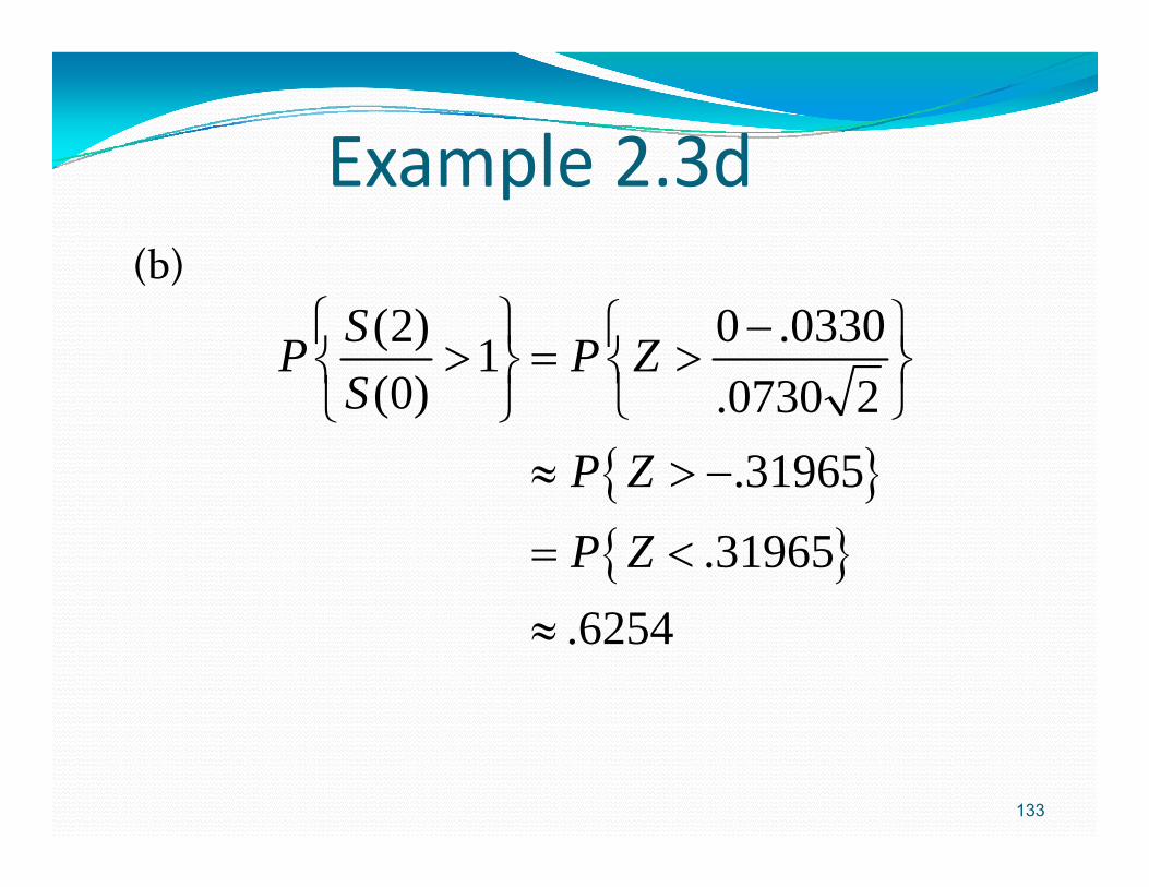
Example 2 3dExample 2.3d(b)(b)

(2) 0 .03301(0) 0730 2

SP P ZS

(0) .0730 2.31965

SP Z

.31965

62 4P Z

.6254

133

Section 2.4h l hThe Central Limit Theorem

134

M k ’ I litMarkov’s InequalitySuppose X is a non negative RV withSuppose X is a non-negative RV with finite mean. Then for any a>0

E XP X a P X a

a

M k ’ I litMarkov’s InequalityProof: Let I = I{X≥a} be the indicator function.Proof: Let I I{X≥a} be the indicator function.

since 0XI Xa

a

[ ]E XE I

( 1) ( )

E Ia

E I P I P X a

[ ]( ) E XP X aa

M k ’ I litMarkov’s InequalityExample: The average amount of waiting time at p g ga post office is 5 minutes. Estimate the probability that you have to wait more than 20 minutes.

[ ] 5( 20) .25E XP X ( 20) .2520 20

P X

Chebyshev’s InequalityS  th t X i    RV  ith fi it    Suppose that X is a RV with finite mean and finite variance. The for any k > 0,

2

1| |P X kk

1| | 1P X k 2| | 1P X kk

Chebyshev’s InequalityChebyshev s InequalityProof:

22

2

( )| | XP X k P k

2

2

| |

XE

2

E

k

2

XVar

k

2

2

1k

k

k

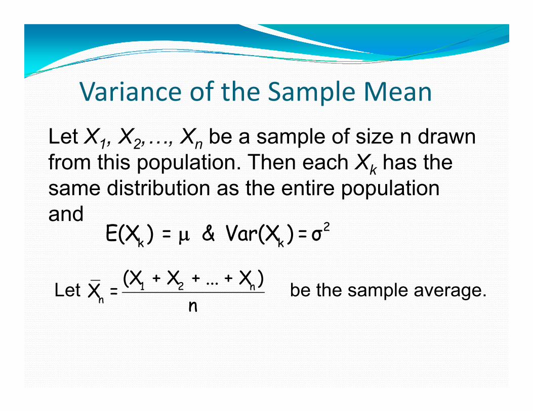
Variance of the Sample Mean

Let X1, X2,…, Xn be a sample of size n drawn from this population. Then each Xk has the same distribution as the entire population and

2E(X ) = & Var(X ) = σk kE(X ) = & Var(X ) = σ

L t b th l1 2(X + X + ... + X ) Let be the sample average. 1 2 n

n

(X X ... X )X =

n

Variance of the Sample MeanVariance of the Sample MeanBy linearity of expectatio E(X ) = μ

When X1, X2,…, Xn are drawn with

By linearity of expectatio E(X ) μn

When X1, X2,…, Xn are drawn with replacement, they are independent and each Xk has variance σ2. ThenXk has variance σ . Then

2 2nσ σ σ Var(X ) = = SD(X ) = n n2 Var(X ) = = SD(X ) = nn n

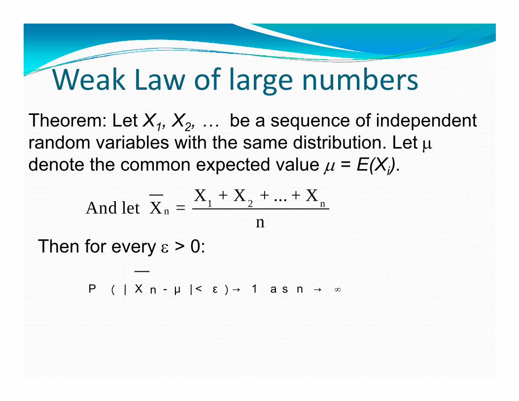
W k L f l bWeak Law of large numbersTheorem: Let X1, X2, … be a sequence of independentTheorem: Let X1, X2, … be a sequence of independent random variables with the same distribution. Let denote the common expected value = E(Xi).

1 2 nn

X + X + ... + XAnd let X =

nThen for every > 0:

n

nP ︵ | X - μ | < ε ︶→ 1 a s n → ∞

Weak Law of large numbersWeak Law of large numbersProof: Let μ = E(Xi) and σ = SD(Xi). ThenProof: Let μ  E(Xi) and σ  SD(Xi). Then

n nσE(X ) = μ and SD(X ) = .n

Apply Chebyshev’s inequality to  

n

nX

2

n nnP |X | P |X |

For a fixed ε right hand side tends to 0 as n tends 

n n

For a fixed ε right hand side tends to 0 as n tends to infinity. 

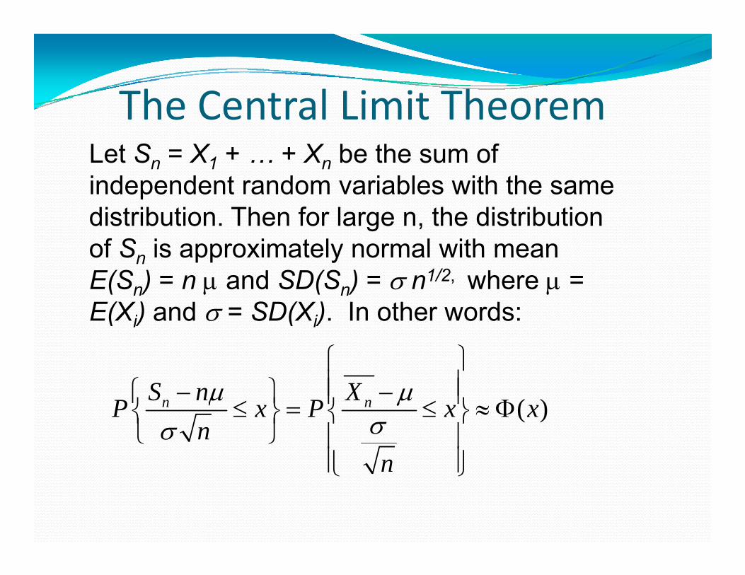
The Central Limit TheoremThe Central Limit TheoremLet Sn = X1 + … + Xn be the sum of i d d t d i bl ith thindependent random variables with the same distribution. Then for large n, the distribution of S is approximately normal with meanof Sn is approximately normal with mean E(Sn) = n and SD(Sn) = n1/2, where = E(Xi) and = SD(Xi). In other words:( i) ( i)

S n X ( )n nS n XP x P x x

nn

n

The Central Limit TheoremThe Central Limit TheoremGiven:

1. The random variable x has a distribution (which may or may not be normal) with (which may or may not be normal) with mean µ and standard deviation . Si l   d   l   ll  f  i    2. Simple random samples all of size n are selected from the population.  (The samples   l t d   th t  ll  ibl   l   f are selected so that all possible samples of 

the same size n have the same chance of being selected )being selected.)

Central Limit Theorem - contConclusions:

Central Limit Theorem - cont

1. The distribution of sample x will, as the sample size increases, approach a normal distribution.

2. The mean of the sample means is the population mean µ.

3. The standard deviation of all sample means is n

P ti l R l C l U dPractical Rules Commonly Used1. For samples of size n larger than 30, the gdistribution of the sample means can be approximated reasonably well by a normal distribution.  The approximation gets better as the sample size n becomes larger.

2. If the original population is itself normally distributed  then the sample means will be distributed, then the sample means will be normally distributed for any sample size n(not just the values of n larger than 30)  (not just the values of n larger than 30). 

Binomial Probability DistributionBinomial Probability Distribution

1. The procedure must have fixed number of trials.

2  The trials must be independent2. The trials must be independent.

3. Each trial must have all outcomes classified into two  categoriescategories.

4. The probability of success remains the same in all trialstrials.

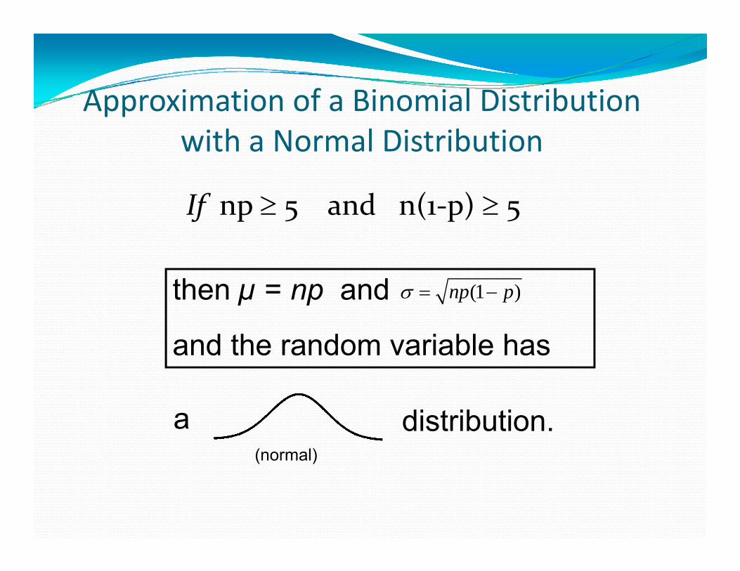
Approximation of a Binomial DistributionApproximation of a Binomial Distributionwith a Normal Distribution

If  np  5    and   n(1‐p)  5

then µ = np and (1 )np p

and the random variable has

distribution.(normal)

a

Example 2 4aExample 2.4aA fair coin is tossed 100 times  What is the A fair coin is tossed 100 times. What is the probability that heads appears fewer than 40 times?40 times?

S l ti  If X denotes the number of heads  Solution. If X denotes the number of heads, then X is a binomial random variable with parameters n   100 and p   1/2  Since np   parameters n = 100 and p = 1/2. Since np = 50 ≥ 5 we have np(1‐ p) = 25 ≥ 5, and so

150

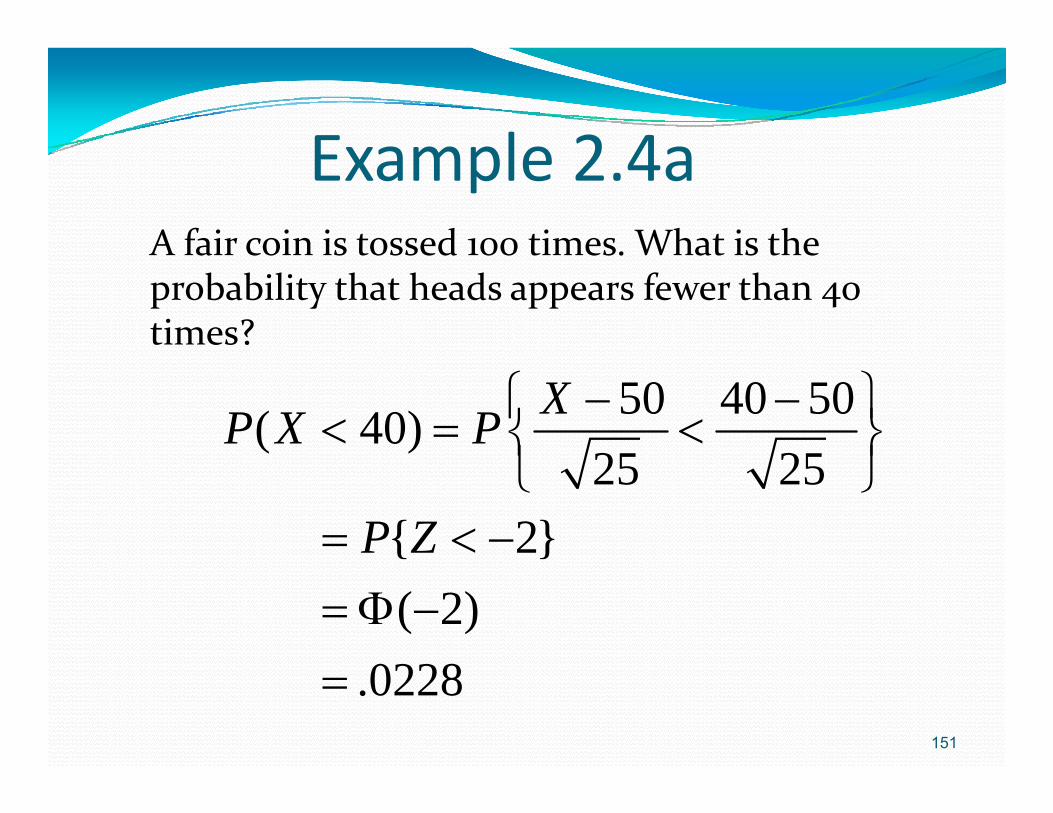
Example 2 4aExample 2.4aA fair coin is tossed 100 times. What is the A fair coin is tossed 100 times. What is the probability that heads appears fewer than 40 times?

50 40 50( 40)25 25

XP X P 25 25

{ 2}P Z

{ }( 2)

151

.0228

Example 2 4aExample 2.4aA graphic calculator computing binomial A graphic calculator computing binomial probabilities gives the exact solution 0176  and so the preceding is not quite as .0176, and so the preceding is not quite as accurate as we might like. However, we could improve the approximation by could improve the approximation by using continuity correction: Write desired probability as P{X < 39 5}  This givesprobability as P{X < 39.5}. This gives

152

Example 2 4aExample 2.4a

50 39.5 50( 39.5)25 25

XP X P 25 25

{ 2.10}P Z

( 2.10)

0179

.0179

153