Review of Adult Lead Models. Evaluation of Models for ... · PDF fileNON-RESIDENTIAL AREAS OF SUPERFUND ... The Technical Review Workgroup for Lead ... 1.4 Model Review Criteria and

EPA OSWER #9285.7-46

August 2001

REVIEW OF ADULT LEAD MODELSEVALUATION OF MODELS FOR

ASSESSING HUMAN HEALTH RISKSASSOCIATED WITH LEAD EXPOSURES AT NON-RESIDENTIAL AREAS OF SUPERFUND

AND OTHER HAZARDOUS WASTE SITES

Office of Solid Waste and Emergency Response U.S. Environmental Protection Agency

Washington, DC 20460

NOTICE

This document provides guidance to EPA staff. It also provides guidance to the public and to the regulated community on how EPA intends to exercise its discretion in implementing the National Contingency Plan. The guidance is designed to implement national policy on these issues. The document does not, however, substitute for EPA's statutes or regulations, nor is it a regulation itself. Thus, it cannot impose legally-binding requirements on EPA, States, or the regulated community, and may not apply to a particular situation based upon the circumstances. EPA may change this guidance in the future, as appropriate.

CONTRIBUTING MEMBERS OF ADULT PB SUB-COMMITTEE OF

U.S. ENVIRONMENTAL PROTECTION AGENCY

TECHNICAL REVIEW WORKGROUP FOR LEAD

The Technical Review Workgroup for Lead (TRW) is an interoffice workgroup convened by the U.S. EPA Office of Solid Waste and Emergency Response/Office of Emergency and Remedial Response (OSWER/OERR).

CHAIRPERSON

Region 2 Mark Maddaloni New York, NY

MEMBERS

Region 1 Region 5 Mary Ballew Patricia VanLeeuwen Boston, MA Chicago, IL

Region 4 Region 6 Kevin Koporec Ghassan Khoury Atlanta, GA Dallas, TX

Region 5 OERR Mentor Mark Johnson Larry Zaragoza

Office of Emergency and Remedial Response Washington, DC

Chicago, IL

Review of Adult Lead Models Evaluation of Models for Assessing Human Health Risks Associated with Lead Exposures at Non-Residential Areas of Superfund and Other Hazardous Waste Sites

Final Draft: August 2001

Prepared by the

Adult Lead Risk Assessment Committee of the Technical Review Workgroup for Lead (TRW)

NOTICE

This document has been reviewed in accordance with U.S. EPA policy and is approved for publication. Mention of trade names or commercial products does not constitute endorsement of recommendation.

ii REVIEW OF ADU LT LEAD MODELS

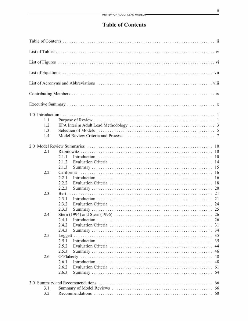
Table of Contents

Table of Contents . . . . . . . . . . . . . . . . . . . . . . . . . . . . . . . . . . . . . . . . . . . . . . . . . . . . . . . . . . . . . . . . . . . . ii

List of Tables . . . . . . . . . . . . . . . . . . . . . . . . . . . . . . . . . . . . . . . . . . . . . . . . . . . . . . . . . . . . . . . . . . . . . . . iv

List of Figures . . . . . . . . . . . . . . . . . . . . . . . . . . . . . . . . . . . . . . . . . . . . . . . . . . . . . . . . . . . . . . . . . . . . . . vi

List of Equations . . . . . . . . . . . . . . . . . . . . . . . . . . . . . . . . . . . . . . . . . . . . . . . . . . . . . . . . . . . . . . . . . . . vii

List of Acronyms and Abbreviations . . . . . . . . . . . . . . . . . . . . . . . . . . . . . . . . . . . . . . . . . . . . . . . . . . . . viii

Contributing Members . . . . . . . . . . . . . . . . . . . . . . . . . . . . . . . . . . . . . . . . . . . . . . . . . . . . . . . . . . . . . . . . ix

Executive Summary . . . . . . . . . . . . . . . . . . . . . . . . . . . . . . . . . . . . . . . . . . . . . . . . . . . . . . . . . . . . . . . . . . x

1.0 Introduction . . . . . . . . . . . . . . . . . . . . . . . . . . . . . . . . . . . . . . . . . . . . . . . . . . . . . . . . . . . . . . . . . . . . . 1 1.1 Purpose of Review . . . . . . . . . . . . . . . . . . . . . . . . . . . . . . . . . . . . . . . . . . . . . . . . . . . . . . 1 1.2 EPA Interim Adult Lead Methodology . . . . . . . . . . . . . . . . . . . . . . . . . . . . . . . . . . . . . . 3 1.3 Selection of Models . . . . . . . . . . . . . . . . . . . . . . . . . . . . . . . . . . . . . . . . . . . . . . . . . . . . . 5 1.4 Model Review Criteria and Process . . . . . . . . . . . . . . . . . . . . . . . . . . . . . . . . . . . . . . . . 7

2.0 Model Review Summaries . . . . . . . . . . . . . . . . . . . . . . . . . . . . . . . . . . . . . . . . . . . . . . . . . . . . . . . . 10 2.1 Rabinowitz . . . . . . . . . . . . . . . . . . . . . . . . . . . . . . . . . . . . . . . . . . . . . . . . . . . . . . . . . . . 10

2.1.1 Introduction . . . . . . . . . . . . . . . . . . . . . . . . . . . . . . . . . . . . . . . . . . . . . . . . . . . . 10 2.1.2 Evaluation Criteria . . . . . . . . . . . . . . . . . . . . . . . . . . . . . . . . . . . . . . . . . . . . . . 14 2.1.3 Summary . . . . . . . . . . . . . . . . . . . . . . . . . . . . . . . . . . . . . . . . . . . . . . . . . . . . . . 15

2.2 California . . . . . . . . . . . . . . . . . . . . . . . . . . . . . . . . . . . . . . . . . . . . . . . . . . . . . . . . . . . 16 2.2.1 Introduction . . . . . . . . . . . . . . . . . . . . . . . . . . . . . . . . . . . . . . . . . . . . . . . . . . . . 16 2.2.2 Evaluation Criteria . . . . . . . . . . . . . . . . . . . . . . . . . . . . . . . . . . . . . . . . . . . . . . 18 2.2.3 Summary . . . . . . . . . . . . . . . . . . . . . . . . . . . . . . . . . . . . . . . . . . . . . . . . . . . . . . 20

2.3 Bert . . . . . . . . . . . . . . . . . . . . . . . . . . . . . . . . . . . . . . . . . . . . . . . . . . . . . . . . . . . . . . . . 21 2.3.1 Introduction . . . . . . . . . . . . . . . . . . . . . . . . . . . . . . . . . . . . . . . . . . . . . . . . . . . . 21 2.3.2 Evaluation Criteria . . . . . . . . . . . . . . . . . . . . . . . . . . . . . . . . . . . . . . . . . . . . . . 24 2.3.3 Summary . . . . . . . . . . . . . . . . . . . . . . . . . . . . . . . . . . . . . . . . . . . . . . . . . . . . . . 25

2.4 Stern (1994) and Stern (1996) . . . . . . . . . . . . . . . . . . . . . . . . . . . . . . . . . . . . . . . . . . . . 26 2.4.1 Introduction . . . . . . . . . . . . . . . . . . . . . . . . . . . . . . . . . . . . . . . . . . . . . . . . . . . . 26 2.4.2 Evaluation Criteria . . . . . . . . . . . . . . . . . . . . . . . . . . . . . . . . . . . . . . . . . . . . . . 31 2.4.3 Summary . . . . . . . . . . . . . . . . . . . . . . . . . . . . . . . . . . . . . . . . . . . . . . . . . . . . . . 34

2.5 Leggett . . . . . . . . . . . . . . . . . . . . . . . . . . . . . . . . . . . . . . . . . . . . . . . . . . . . . . . . . . . . . . 35 2.5.1 Introduction . . . . . . . . . . . . . . . . . . . . . . . . . . . . . . . . . . . . . . . . . . . . . . . . . . . . 35 2.5.2 Evaluation Criteria . . . . . . . . . . . . . . . . . . . . . . . . . . . . . . . . . . . . . . . . . . . . . . 44 2.5.3 Summary . . . . . . . . . . . . . . . . . . . . . . . . . . . . . . . . . . . . . . . . . . . . . . . . . . . . . . 46

2.6 O’Flaherty . . . . . . . . . . . . . . . . . . . . . . . . . . . . . . . . . . . . . . . . . . . . . . . . . . . . . . . . . . . 48 2.6.1 Introduction . . . . . . . . . . . . . . . . . . . . . . . . . . . . . . . . . . . . . . . . . . . . . . . . . . . . 48 2.6.2 Evaluation Criteria . . . . . . . . . . . . . . . . . . . . . . . . . . . . . . . . . . . . . . . . . . . . . . 61 2.6.3 Summary . . . . . . . . . . . . . . . . . . . . . . . . . . . . . . . . . . . . . . . . . . . . . . . . . . . . . . 64

3.0 Summary and Recommendations . . . . . . . . . . . . . . . . . . . . . . . . . . . . . . . . . . . . . . . . . . . . . . . . . . . 66 3.1 Summary of Model Reviews . . . . . . . . . . . . . . . . . . . . . . . . . . . . . . . . . . . . . . . . . . . . . 66 3.2 Recommendations . . . . . . . . . . . . . . . . . . . . . . . . . . . . . . . . . . . . . . . . . . . . . . . . . . . . . 68

iii REVIEW OF ADU LT LEAD MODELS

4.0 References . . . . . . . . . . . . . . . . . . . . . . . . . . . . . . . . . . . . . . . . . . . . . . . . . . . . . . . . . . . . . . . . . . . . . 70

Appendix A. Comparison of Gastrointestinal Absorption Factors in Leggett and O'Flaherty Models . . . . . . . . . . . . . . . . . . . . . . . . . . . . . . . . . . . . . . . . . . . . . . . . . . . . . . . . . . . . . A-1

Appendix B. Comparison of Biokinetic Slope Factors (BKSF) for Children Predicted by the IEUBK Model and O’Flaherty Model . . . . . . . . . . . . . . . . . . . . . . . . . . . . . . . . . . . . . B-1

Appendix C. Biokinetic Slope Factors (BKSF) for Adults Predicted by the O’Flaherty Model . . . C-1

Appendix D. Comparison of Biokinetic Slope Factors (BKSF) for Children Predicted by the IEUBK Model and Leggett Models . . . . . . . . . . . . . . . . . . . . . . . . . . . . . . . . . . . . . . . D-1

Appendix E. Biokinetic Slope Factor (BKSF) for Adults Predicted by the Leggett Model . . . . . . . E-1

Appendix F. Modeling of Bone Lead and Bone Metabolism During Adolescence - O’Flaherty Model . . . . . . . . . . . . . . . . . . . . . . . . . . . . . . . . . . . . . . . . . . . . . . . . . . . . . . . . . . . . . . . F-1

Appendix G. Miscellaneous Issues Related to the O’Flaherty Model ACSL Code . . . . . . . . . . . . . G-1

Appendix H. Miscellaneous Issues Related to the O’Flaherty Model C++ Code . . . . . . . . . . . . . . . H-1

Appendix I. Mass Balance in O’Flaherty Model . . . . . . . . . . . . . . . . . . . . . . . . . . . . . . . . . . . . . . . . I-1

Appendix J. Comparisons of Blood Lead Concentrations Predicted by the Leggett Model and the EPA ALM . . . . . . . . . . . . . . . . . . . . . . . . . . . . . . . . . . . . . . . . . . . . . . . . . . . . . . . . J-1

Appendix K. Comparisons of Blood Lead Concentrations Predicted by the O’Flaherty Model and the EPA ALM . . . . . . . . . . . . . . . . . . . . . . . . . . . . . . . . . . . . . . . . . . . . . . . . . . . . . . . K-1

Appendix L. Comparisons of Blood Lead Concentrations Predicted by the Bert Model and the EPA ALM . . . . . . . . . . . . . . . . . . . . . . . . . . . . . . . . . . . . . . . . . . . . . . . . . . . . . . . . . . L-1

iv REVIEW OF ADU LT LEAD MODELS

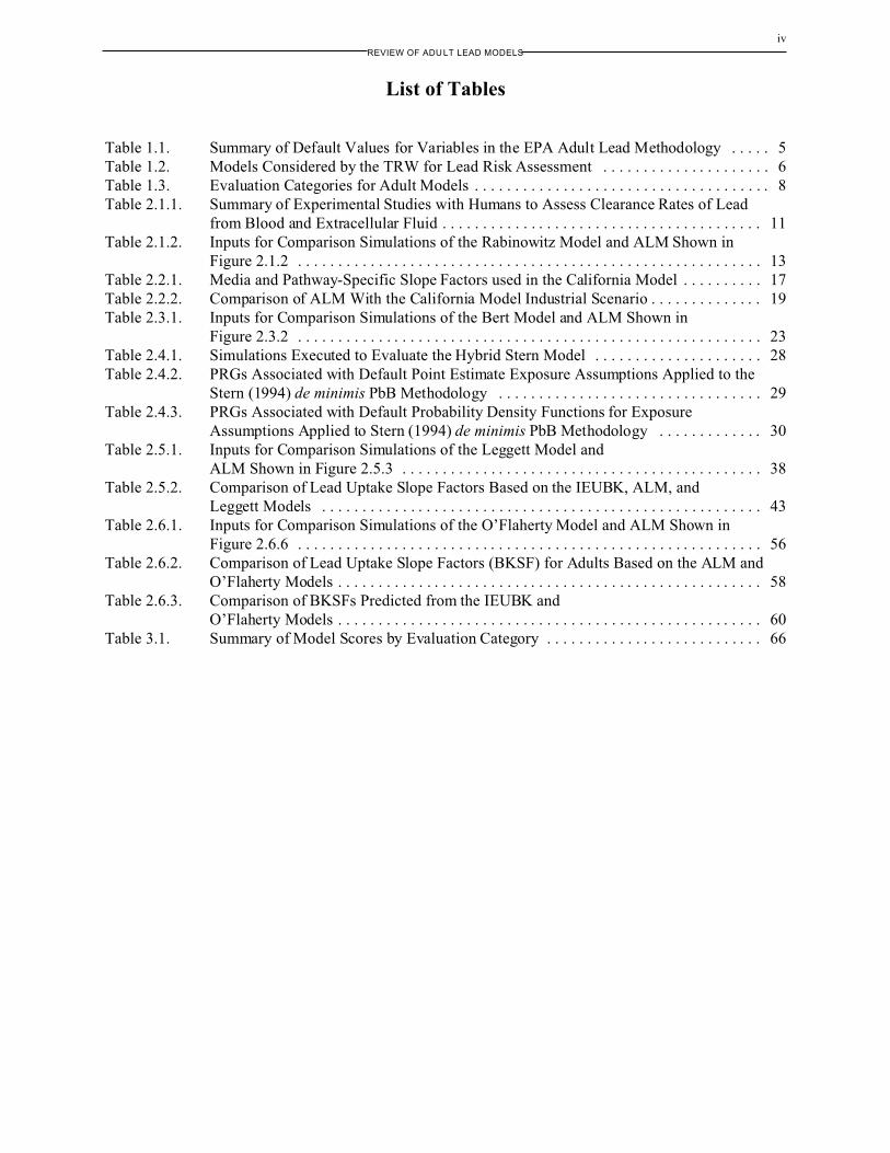
List of Tables

Table 1.1. Summary of Default Values for Variables in the EPA Adult Lead Methodology . . . . . 5 Table 1.2. Models Considered by the TRW for Lead Risk Assessment . . . . . . . . . . . . . . . . . . . . . 6 Table 1.3. Evaluation Categories for Adult Models . . . . . . . . . . . . . . . . . . . . . . . . . . . . . . . . . . . . . 8 Table 2.1.1. Summary of Experimental Studies with Humans to Assess Clearance Rates of Lead

from Blood and Extracellular Fluid . . . . . . . . . . . . . . . . . . . . . . . . . . . . . . . . . . . . . . . . 11 Table 2.1.2. Inputs for Comparison Simulations of the Rabinowitz Model and ALM Shown in

Figure 2.1.2 . . . . . . . . . . . . . . . . . . . . . . . . . . . . . . . . . . . . . . . . . . . . . . . . . . . . . . . . . . 13 Table 2.2.1. Media and Pathway-Specific Slope Factors used in the California Model . . . . . . . . . . 17 Table 2.2.2. Comparison of ALM With the California Model Industrial Scenario . . . . . . . . . . . . . . 19 Table 2.3.1. Inputs for Comparison Simulations of the Bert Model and ALM Shown in

Figure 2.3.2 . . . . . . . . . . . . . . . . . . . . . . . . . . . . . . . . . . . . . . . . . . . . . . . . . . . . . . . . . . 23 Table 2.4.1. Simulations Executed to Evaluate the Hybrid Stern Model . . . . . . . . . . . . . . . . . . . . . 28 Table 2.4.2. PRGs Associated with Default Point Estimate Exposure Assumptions Applied to the

Stern (1994) de minimis PbB Methodology . . . . . . . . . . . . . . . . . . . . . . . . . . . . . . . . . 29 Table 2.4.3. PRGs Associated with Default Probability Density Functions for Exposure

Assumptions Applied to Stern (1994) de minimis PbB Methodology . . . . . . . . . . . . . 30 Table 2.5.1. Inputs for Comparison Simulations of the Leggett Model and

ALM Shown in Figure 2.5.3 . . . . . . . . . . . . . . . . . . . . . . . . . . . . . . . . . . . . . . . . . . . . . 38 Table 2.5.2. Comparison of Lead Uptake Slope Factors Based on the IEUBK, ALM, and

Leggett Models . . . . . . . . . . . . . . . . . . . . . . . . . . . . . . . . . . . . . . . . . . . . . . . . . . . . . . . 43 Table 2.6.1. Inputs for Comparison Simulations of the O’Flaherty Model and ALM Shown in

Figure 2.6.6 . . . . . . . . . . . . . . . . . . . . . . . . . . . . . . . . . . . . . . . . . . . . . . . . . . . . . . . . . . 56 Table 2.6.2. Comparison of Lead Uptake Slope Factors (BKSF) for Adults Based on the ALM and

O’Flaherty Models . . . . . . . . . . . . . . . . . . . . . . . . . . . . . . . . . . . . . . . . . . . . . . . . . . . . . 58 Table 2.6.3. Comparison of BKSFs Predicted from the IEUBK and

O’Flaherty Models . . . . . . . . . . . . . . . . . . . . . . . . . . . . . . . . . . . . . . . . . . . . . . . . . . . . . 60 Table 3.1. Summary of Model Scores by Evaluation Category . . . . . . . . . . . . . . . . . . . . . . . . . . . 66

v REVIEW OF ADU LT LEAD MODELS

List of Figures

Figure 1.1. Decision Tree for Evaluating Alternative Models in Terms of Options for Retaining, Replacing, or Modifying the Adult Methodology . . . . . . . . . . . . . . . . . . . . . . . . . . . . . . 2

Figure 2.1.1. Rabinowitz et al. (1976) BIOKINETIC MODEL FOR LEAD . . . . . . . . . . . . . . . . . . . . . . . . 11 Figure 2.1.2. Comparison of Blood Lead Concentrations Predicted by the Rabinowitz Model and

ALM . . . . . . . . . . . . . . . . . . . . . . . . . . . . . . . . . . . . . . . . . . . . . . . . . . . . . . . . . . . . . . . . 14 Figure 2.2.1. Conceptual Model of Lead Exposure and

Biokinetics in the California Model . . . . . . . . . . . . . . . . . . . . . . . . . . . . . . . . . . . . . . . 16 Figure 2.3.1. Lead Body Burden Associated with Intakes of Lead to the Gastrointestinal and

Respiratory Tracts for a Typical Adult Male . . . . . . . . . . . . . . . . . . . . . . . . . . . . . . . . . 21 Figure 2.3.2. Comparison of Blood Lead Concentration Predicted

by the Bert Model and the ALM . . . . . . . . . . . . . . . . . . . . . . . . . . . . . . . . . . . . . . . . . . 24 Figure 2.4.1. Cumulative Probability Distribution (CDF) of Output from Hybrid Stern Model,

Using Stern (1994) de minimis Blood Lead Concentration Model with Stern (1996) Adult Inputs for PDF . . . . . . . . . . . . . . . . . . . . . . . . . . . . . . . . . . . . . . . . . . . . . . . . . . . 32

Figure 2.4.2. Comparison of Soil Lead Concentrations (PRGs) Using EPA (1996) ALM and Probabilistic Stern Model (See Table 2.4.3) as a Function of Baseline Blood Lead Concentrations (PbB0) . . . . . . . . . . . . . . . . . . . . . . . . . . . . . . . . . . . . . . . . . . . . . . . . . . 33

Figure 2.5.1. Schematic of the Biokinetic Model of Lead Metabolism Proposed by Leggett (1993) 36 Figure 2.5.2. Default Values in the Leggett Model for Lead Absorption in the Gastrointestinal

Tract (Percent) as a Function of Age . . . . . . . . . . . . . . . . . . . . . . . . . . . . . . . . . . . . . . . 38 Figure 2.5.3. Comparison of Blood Lead Concentrations Predicted by the Leggett Model and

ALM . . . . . . . . . . . . . . . . . . . . . . . . . . . . . . . . . . . . . . . . . . . . . . . . . . . . . . . . . . . . . . . . 40 Figure 2.5.4a. Leggett Model Simulation of Baseline Blood Lead Concentration and Cortical and

Trabecular Bone Lead . . . . . . . . . . . . . . . . . . . . . . . . . . . . . . . . . . . . . . . . . . . . . . . . . . 41 Figure 2.5.4b. Leggett Model Simulation of Baseline Blood Lead Concentration . . . . . . . . . . . . . . . . 42 Figure 2.5.5. Biokinetic Slope Factors (BKSFs) for Adults Predicted by the Leggett Model . . . . . . 43 Figure 2.6.1. Compartments and Pathways of Lead Exchange in the O’Flaherty Model . . . . . . . . . . 51 Figure 2.6.2. Bone Volume-Age Relationships for Human Juvenile and

Mature Bone as Represented in the O’Flaherty Model . . . . . . . . . . . . . . . . . . . . . . . . . 53 Figure 2.6.3. Bone Volume-Age Relationships for Human Juvenile Cortical and Trabecular Bone

as Represented in the O’Flaherty Model . . . . . . . . . . . . . . . . . . . . . . . . . . . . . . . . . . . . 54 Figure 2.6.4. Default Values for Gastrointestinal Lead Absorption as a Function of Age as

Simulated in the O’Flaherty Model . . . . . . . . . . . . . . . . . . . . . . . . . . . . . . . . . . . . . . . . 55 Figure 2.6.5. O’Flaherty Model Simulation of Baseline Blood Lead (PbB) Concentration . . . . . . . . 57 Figure 2.6.6. Comparison of Blood Lead Concentration Predicted by the O’Flaherty Model and

ALM . . . . . . . . . . . . . . . . . . . . . . . . . . . . . . . . . . . . . . . . . . . . . . . . . . . . . . . . . . . . . . . . 59 Figure 2.6.7. Biokinetic Slope Factors for Adults Predicted by the O’Flaherty Model . . . . . . . . . . . 61

vi REVIEW OF ADU LT LEAD MODELS

List of Equations

Equation 1.2.1 . . . . . . . . . . . . . . . . . . . . . . . . . . . . . . . . . . . . . . . . . . . . . . . . . . . . . . . . . . . . . . . . . . . . . . 3 Equation 1.2.2 . . . . . . . . . . . . . . . . . . . . . . . . . . . . . . . . . . . . . . . . . . . . . . . . . . . . . . . . . . . . . . . . . . . . . . 3 Equation 1.3.1 . . . . . . . . . . . . . . . . . . . . . . . . . . . . . . . . . . . . . . . . . . . . . . . . . . . . . . . . . . . . . . . . . . . . . . 6 Equation 1.3.2 . . . . . . . . . . . . . . . . . . . . . . . . . . . . . . . . . . . . . . . . . . . . . . . . . . . . . . . . . . . . . . . . . . . . . . 6 Equation 1.3.3 . . . . . . . . . . . . . . . . . . . . . . . . . . . . . . . . . . . . . . . . . . . . . . . . . . . . . . . . . . . . . . . . . . . . . . 6 Equation 2.4.1 . . . . . . . . . . . . . . . . . . . . . . . . . . . . . . . . . . . . . . . . . . . . . . . . . . . . . . . . . . . . . . . . . . . . . 26 Equation 2.4.2 . . . . . . . . . . . . . . . . . . . . . . . . . . . . . . . . . . . . . . . . . . . . . . . . . . . . . . . . . . . . . . . . . . . . . 26 Equation 2.4.3 . . . . . . . . . . . . . . . . . . . . . . . . . . . . . . . . . . . . . . . . . . . . . . . . . . . . . . . . . . . . . . . . . . . . . 27 Equation 2.4.4 . . . . . . . . . . . . . . . . . . . . . . . . . . . . . . . . . . . . . . . . . . . . . . . . . . . . . . . . . . . . . . . . . . . . . 31 Equation 2.6.1 . . . . . . . . . . . . . . . . . . . . . . . . . . . . . . . . . . . . . . . . . . . . . . . . . . . . . . . . . . . . . . . . . . . . . 48 Equation 2.6.2 . . . . . . . . . . . . . . . . . . . . . . . . . . . . . . . . . . . . . . . . . . . . . . . . . . . . . . . . . . . . . . . . . . . . . 48 Equation 2.6.3 . . . . . . . . . . . . . . . . . . . . . . . . . . . . . . . . . . . . . . . . . . . . . . . . . . . . . . . . . . . . . . . . . . . . . 48 Equation 2.6.4 . . . . . . . . . . . . . . . . . . . . . . . . . . . . . . . . . . . . . . . . . . . . . . . . . . . . . . . . . . . . . . . . . . . . . 48 Equation 2.6.5 . . . . . . . . . . . . . . . . . . . . . . . . . . . . . . . . . . . . . . . . . . . . . . . . . . . . . . . . . . . . . . . . . . . . . 49 Equation 2.6.6 . . . . . . . . . . . . . . . . . . . . . . . . . . . . . . . . . . . . . . . . . . . . . . . . . . . . . . . . . . . . . . . . . . . . . 53

vii REVIEW OF ADU LT LEAD MODELS

List of Acronyms and Abbreviations

ACSL . . . . . . . . . . . . . . . . . . . . . . . . . . . . . . . . . . . . . . . . . . . Advanced Continuous Simulation Language AF . . . . . . . . . . . . . . . . . . . . . . . . . . . . . . . . . . . . . . . . . . . . . . . . . . . . . . . . . . . . . . . . . absorption fraction ALM . . . . . . . . . . . . . . . . . . . . . . . . . . . . . . . . . . . . . . . . . . . . . . . . . . . . . . . . . . . Adult Lead Methodology AM . . . . . . . . . . . . . . . . . . . . . . . . . . . . . . . . . . . . . . . . . . . . . . . . . . . . . . . . . . . . . . . . . . . arithmetic mean BKSF . . . . . . . . . . . . . . . . . . . . . . . . . . . . . . . . . . . . . . . . . . . . . . . . . . . . . . . . . . . . biokinetic slope factor ED . . . . . . . . . . . . . . . . . . . . . . . . . . . . . . . . . . . . . . . . . . . . . . . . . . . . . . . . . . . . . . . . . . exposure duration EF . . . . . . . . . . . . . . . . . . . . . . . . . . . . . . . . . . . . . . . . . . . . . . . . . . . . . . . . . . . . . . . . . . exposure frequency EPA . . . . . . . . . . . . . . . . . . . . . . . . . . . . . . . . . . . . . . . . . . . . . . . . . . . . Environmental Protection Agency GM . . . . . . . . . . . . . . . . . . . . . . . . . . . . . . . . . . . . . . . . . . . . . . . . . . . . . . . . . . . . . . . . . . . . geometric mean GSD . . . . . . . . . . . . . . . . . . . . . . . . . . . . . . . . . . . . . . . . . . . . . . . . . . . . . . . . geometric standard deviation IEUBK . . . . . . . . . . . . . . . . . . . . . . . Integrated Exposure Uptake Biokinetic Model for Lead in Children IR . . . . . . . . . . . . . . . . . . . . . . . . . . . . . . . . . . . . . . . . . . . . . . . . . . . . . . . . . . . . . . . . . . . . . . ingestion rate NHANES . . . . . . . . . . . . . . . . . . . . . . . . . . . . . . . . . . National Health and Nutrition Examination Survey ORD . . . . . . . . . . . . . . . . . . . . . . . . . . . . . . . . . . . . . . . . . . . . . . . . . . Office of Research and Development Pb . . . . . . . . . . . . . . . . . . . . . . . . . . . . . . . . . . . . . . . . . . . . . . . . . . . . . . . . . . . . . . . . . . . . . . . . . . . . . . lead PbB . . . . . . . . . . . . . . . . . . . . . . . . . . . . . . . . . . . . . . . . . . . . . . . . . . . . . . . . . . . . . . . . . . . . . . . . blood lead PbB0 . . . . . . . . . . . . . . . . . . . . . . . . . . . . . . . . . . . . . . . . . . . . . . . . . . . . . . . . . . . . . . . . baseline blood lead PbS . . . . . . . . . . . . . . . . . . . . . . . . . . . . . . . . . . . . . . . . . . . . . . . . . . . . . . . . . . . . . . . . . . . . . . . . . . soil lead PDF . . . . . . . . . . . . . . . . . . . . . . . . . . . . . . . . . . . . . . . . . . . . . . . . . . . . . . probability distribution function PRG . . . . . . . . . . . . . . . . . . . . . . . . . . . . . . . . . . . . . . . . . . . . . . . . . . . . . . . . preliminary remediation goal RAF . . . . . . . . . . . . . . . . . . . . . . . . . . . . . . . . . . . . . . . . . . . . . . . . . . . . . . . . . . relative absorption fraction SF . . . . . . . . . . . . . . . . . . . . . . . . . . . . . . . . . . . . . . . . . . . . . . . . . . . . . . . . . . . . . . . . . . . . . . . . slope factor TRW . . . . . . . . . . . . . . . . . . . . . . . . . . . . . . . . . . . . . . . . . . . . . . . . Technical Review Workgroup for Lead

% . . . . . . . . . . . . . . . . . . . . . . . . . . . . . . . . . . . . . . . . . . . . . . . . . . . . . . . . . . . . . . . . . . . . . . . . . . . percent � . . . . . . . . . . . . . . . . . . . . . . . . . . . . . . . . . . . . . . . . . . . . . . . . . . . . . . . . . . . . . . . . . . . . . . . . . . . . . . delta �g . . . . . . . . . . . . . . . . . . . . . . . . . . . . . . . . . . . . . . . . . . . . . . . . . . . . . . . . . . . . . . . . . . . . . . . . . microgram d . . . . . . . . . . . . . . . . . . . . . . . . . . . . . . . . . . . . . . . . . . . . . . . . . . . . . . . . . . . . . . . . . . . . . . . . . . . . . . . day dL . . . . . . . . . . . . . . . . . . . . . . . . . . . . . . . . . . . . . . . . . . . . . . . . . . . . . . . . . . . . . . . . . . . . . . . . . . . deciliter g . . . . . . . . . . . . . . . . . . . . . . . . . . . . . . . . . . . . . . . . . . . . . . . . . . . . . . . . . . . . . . . . . . . . . . . . . . . . . . gram L . . . . . . . . . . . . . . . . . . . . . . . . . . . . . . . . . . . . . . . . . . . . . . . . . . . . . . . . . . . . . . . . . . . . . . . . . . . . . . . liter m3 . . . . . . . . . . . . . . . . . . . . . . . . . . . . . . . . . . . . . . . . . . . . . . . . . . . . . . . . . . . . . . . . . . . . . . . cubic meters mm . . . . . . . . . . . . . . . . . . . . . . . . . . . . . . . . . . . . . . . . . . . . . . . . . . . . . . . . . . . . . . . . . . . . . . . millimeters mo . . . . . . . . . . . . . . . . . . . . . . . . . . . . . . . . . . . . . . . . . . . . . . . . . . . . . . . . . . . . . . . . . . . . . . . . . . . month ppm . . . . . . . . . . . . . . . . . . . . . . . . . . . . . . . . . . . . . . . . . . . . . . . . . . . . . . . . . . . . . . . . . . parts per million wk . . . . . . . . . . . . . . . . . . . . . . . . . . . . . . . . . . . . . . . . . . . . . . . . . . . . . . . . . . . . . . . . . . . . . . . . . . . . . week yr . . . . . . . . . . . . . . . . . . . . . . . . . . . . . . . . . . . . . . . . . . . . . . . . . . . . . . . . . . . . . . . . . . . . . . . . . . . . . . year

viii REVIEW OF ADU LT LEAD MODELS

Contributing Members of Adult Pb Sub-Committee of U.S. Environmental Protection Agency Technical Review Workgroup for Lead

CHAIR

Mark Maddaloni Region 2 New York, NY

MEMBERS

Mary Ballew Region 1 Boston, MA

Mark Johnson Region 5 Chicago, IL

Ghassan Khoury Region 6 Dallas, TX

Kevin Koporec Region 4 Atlanta, GA

Patricia Van Leeuwen Region 5 Chicago, IL

Larry Zaragoza Office of Emergency and Remedial Response Washington, DC

ix REVIEW OF ADU LT LEAD MODELS

Executive Summary

In 1996, in response to the need for a scientifically defensible approach for assessing human health lead risks at non-residential hazardous waste sites, the U.S. Environmental Protection Agency’s (EPA’s) Technical Review Workgroup for Lead (TRW) developed the Adult Lead Methodology (ALM). The ALM was released by the EPA as an interim report entitled Recommendations of the Technical Review Workgroup for Lead (TRW) for an Interim Approach to Assessing Risks Associated with Adult Exposures to Lead in Soil. The effort to provide interim guidance in a timely manner limited the scope of the approach to adult workers and specific exposure media (i.e., soil/dust). Therefore, as a follow-up to the ALM, a more exhaustive effort was undertaken to evaluate other currently available modeling approaches and their potential applicability to assessing non-residential lead exposures and risks.

This report evaluates six lead biokinetic models that have been published in the peer-reviewed scientific literature. These models have been used to assess the relationship between environmental lead exposures and blood lead (PbB) concentration in adults. Each model was evaluated and compared to the ALM using the following general evaluation criteria:

• Completeness of exposure module • Kinetic performance • Utility of model output • Ease of use and flexibility

This report presents summaries of the model reviews and provides recommendations for whether:

• a superior model is currently available that could replace the existing ALM; • a new model should be developed; • the existing model should be modified; • the ALM should be retained.

The models reviewed were slope factor and multi-compartmental models and included the California Carlisle and Wade (1992), Stern (1994, 1996), Rabinowitz (1976), Bert (1989), Leggett (1993a,b, 1996), and O’Flaherty (1993, 1995) models. All models reviewed showed strengths and weaknesses. The models are discussed in greater detail in subsequent sections of this report. Although no single model reviewed by the TRW was judged to be a significant improvement over the ALM, various components from the different models were determined to offer refinements in adult lead modeling. These components could be integrated into a hybrid model; however, such modifications would require a long-term effort (i.e., months to years). The decision not to proceed with development of a hybrid model is discussed below. However, in lieu of such an effort, it is worth noting that the kinetic performance of all the models produced similar estimates of quasi-steady-state PbB concentrations when exposure parameters were normalized across models (i.e., all were set to approximate ALM inputs).

While model evaluations were being conducted by the TRW, the EPA Office of Research and Development (ORD) initiated an effort to develop an All Ages Lead Model capable of simulating multimedia exposures and biokinetics over the entire human lifespan. The TRW has long contemplated the expansion of the Integrated Exposure Uptake Biokinetic Model for Lead in Children (IEUBK model) to accommodate a wider age range of exposure. Conceptually, the goals of the All Ages Lead Model are similar to the IEUBK model in that it could have an integrated multimedia exposure module and a relatively complex (e.g., multi-compartment) biokinetic module.

x REVIEW OF ADU LT LEAD MODELS

To support the All Ages Lead Model effort and to minimize overlapping of EPA’s goals for developing lead risk assessment models, the TRW elected to direct recommendations for model improvements based on the adult model reviews to the All Ages Lead Model initiative.

Based on the TRW evaluations described in this report and recognition that the All Ages Lead Model is currently under development, the TRW has chosen to retain the ALM as an interim tool for assessing soil-borne lead risks for non-residential exposure scenarios. In addition, to assist users with the application of the ALM, the TRW has prepared a fact sheet providing answers to frequently asked questions and may incorporate modifications to model input parameters as new information becomes available. The TRW recognizes that in specific situations such as: (1) short-term exposures or intermittent exposure scenarios; (2) varied age range (e.g., trespasser, recreational); and (3) and/or multimedia contamination, the risks of lead exposures may be more amenable to assessment by alternative models, such as those described in this report. As previously mentioned, the TRW will provide support to the All Ages Lead Model effort.

1 REVIEW OF ADU LT LEAD MODELS

1.0 Introduction

1.1 PURPO SE OF REVIEW

In December 1996, the Technical Review Workgroup for Lead released the report, Recommendations of the Technical Review Workgroup for Lead (TRW) for an Interim Approach to Assessing Risks Associated with Adult Exposures to Lead in Soil. The report filled a direct need for a scientifically defensible approach for assessing soil-borne lead hazards at non-residential hazardous waste sites. Though the report provided readily available guidance, it limited the scope of the approach to a narrowly defined receptor population (i.e., an adult female worker of child-bearing age at a non-residential site or with non-residential exposure scenarios) and specific media (i.e., soil/dust). The Adult Lead Methodology resulting from this study was offered as an interim approach pending a more detailed effort to identify the most scientifically defensible approach for modeling non-residential lead exposure over a broader age range. In performing a more exhaustive evaluation, the TRW initiated a review of currently existing, peer-reviewed lead biokinetic models. Specifically, as the first objective, the TRW focused on addressing the following options:

• Is there a single existing model that should replace the ALM as the recommended approach for non-residential risk assessment?

• Is there a hybrid model that could be constructed with minimal effort that would represent an improvement?

• Should the ALM be retained as the primary model for assessing risks to adults associated with non-residential lead exposures or should the TRW recommend development of a new model?

The options above formed the basis of a decision tree used to determine whether to retain, replace, or modify the ALM (Figure 1.1).


FIGURE 1.1. DECISION TREE FOR EVALUATING ALTERNATIVE MODELS IN TERMS OF

OPTIONS FOR RETAINING, REPLACING, OR MODIFYING THE ADULT METHODOLOGY

While model evaluations were being conducted by the TRW, the ORD initiated an effort to develop an All Ages Lead Model capable of simulating multimedia exposures and biokinetics over the entire human lifespan. Conceptually, the goals of the All Ages Lead Model are similar to the IEUBK model in that it could have an integrated multimedia exposure module and a relatively complex (e.g., multi-compartment) biokinetic module. To support the All Ages Lead Model effort and to minimize overlapping of EPA’s goals for developing lead risk assessment models, the TRW elected to provide recommendations for model improvements to the All Ages Lead Model initiative.

Specifically, the TRW defined the following additional objectives for the model reviews:

• Identify the research and data needs relevant to achieving an optimal model.

• Identify potentially useful features of other models that might be relevant to the development of the All Ages Lead Model.

In order to provide the detailed information necessary to support the development of the All Ages Lead Model and to provide technical users with specific information regarding how the models were evaluated (e.g., how inputs to the Leggett model were derived in order to create a baseline blood lead concentration), the TRW is preparing several technical appendices to this report. The appendices are internal working documents that are available from the TRW upon request. In addition, the TRW recognizes that environmental models are constantly evolving. To the extent possible, the TRW will review these revised models and address their relative strengths and weaknesses in the technical appendices to this report.


1.2 EPA INTERIM ADULT LEAD METHODOLOGY

The ALM is a modified version of a similar approach, described by Bowers et al. (1994), which was used by EPA Region 8 in the assessment of the California Gulch Superfund site in Colorado (Weston 1995). The ALM uses a biokinetic slope factor (BKSF) to represent lead biokinetics and a relatively simple exposure model in which all exposure pathways, other than soil ingestion, are represented by a background PbB concentration. The model is implemented with the following algorithms:

RBC = PbS = (PbBadult,central,goal - PbBadult,0) • AT Equation (1.2.1)

(BKSF • IRS • AFS • EFS)

PbBadult,central,goal = PbBfetal,0.95,goal Equation (1.2.2)

GSDi,adult • Rfetal/maternal

where:

RBC = risk-based concentration (RBC); soil lead concentration (PbS) that would be estimated to result in a specified central tendency PbB concentrations in adults (i.e., women of child-bearing age) at the site (PbBadult,central,goal) and corresponding 95th percentile fetal PbB concentration (PbB fetal,0.95,goal)

PbBadu lt,0 = typical PbB concentration (�g/dL) in women of child-bearing age at the site in the absence of exposures to the site that is being assessed

PbS = soil lead (�g/g) AT = averaging time; the total period during which soil contact may

occur (365 days/year for continuing long term exposures) BKSF = ratio of (quasi-steady state) increase in typical adult PbB

concentration to average daily lead uptake (�g/dL PbB increase per �g/day lead uptake)

IRS = intake rate of soil, includes both outdoor soil and indoor soil-derived dust (g/day)

AFS = absolute gastrointestinal absorption fraction for ingested lead in soil and lead in dust derived from soil (dimensionless)

EFS = exposure frequency for contact with assessed soils and/or dust derived in part from these soils (days of exposure during the averaging period); exposure frequency can be considered days per year for continuing, long-term exposure

PbBadult, central, goal = goal for central estimate of blood lead concentration (�g/dL) in adults (i.e., women of child-bearing age) that have site exposures; the goal is intended to ensure that PbB fetal, 0.95, goal does not exceed 10 �g/dL

PbBfetal, 0.95, goal = goal for the 95th percentile blood lead concentration (�g/dL) among fetuses of women having exposures to the specified site soil concentration; this is interpreted to mean that there is a 95 percent likelihood that a fetus, in a woman who experiences such exposures, would have a blood lead concentration no greater than PbB fetal, 0.95, goal (i.e., the likelihood of a blood lead con-


centration greater than 10 �g/dL would be less than 5 percent for the approach described in this report)

GSDi, adult = estimated value of the individual geometric standard deviation; the GSD among adults (i.e., women of child-bearing age) that have exposures to similar on-site lead concentrations, but that have non-uniform response (intake, biokinetics) to site lead and non-uniform off-site lead exposures

Rfetal/maternal = constant of proportionality between fetal PbB concentration at birth and maternal PbB concentration.

The default values for the variables in Equations 1.2.1 and 1.2.2 are presented in Table 1.1.


TABLE 1.1. SUMMARY OF DEFAULT VALUES FOR VARIABLES IN THE

EPA ADULT LEAD METHODOLOGYa

Variable Value Unit Comment

PbBfetal, 0.095, goal 10 �g/dL Used to estimate RBC s based on risk to the developing

fetus.

GSDi, adult 1.8– 2.1 – Value of 1.8 is recommended for a homogeneous

population, while 2.1 is recommended for a more

heterogeneous population.

Rfetal/maternal 0.9 – Based on Goyer (1990) and Graziano et al., (1990).

PbBadult, 0 1.7– 2.2 �g/dL Plausible range based on NHANES III phase 1 for

Mexican-American, non-Hispanic black, and white women

of child bear ing age (Brody et al.,199 4). oint estim ate

should b e selected ba sed on site-specific dem ograp hics.

BKSF 0.4 �g/dL per

�g/day

Based on analysis of Pocock et al., (1983) and S herlock et

al., (1984) data.

P

IRS 0.05 g/day Pre dom inantly no n-residential exposures to indoor so il

derived d ust rather than o utdo or so il

(0.05 g/day=50 mg/day).

EFS 219 days/year Based on EPA (1993 ) guidance for average time spent at

work by b oth full-time and part-time work ers.

AFS 0.12 – Based on an ab sorption factor for soluble lead of 0.20 and

a relative bioavialability of 0.6 (soil/soluble).

aVariables refer to Equations 1 and 2 in text, as described in EPA (1996).

1.3 SELEC TION OF MODELS

Seven models were identified from scientific literature searches or brought to the TRW’s attention as the result of reviews of lead risk assessments conducted in the various EPA regions (see Table 1.2). Six models were selected for review by the TRW. The Bowers et al. (1994) model was not included in this review effort, because of the similarity between the Bowers and ALM models. The basic algorithms for the Bowers model were used for the California Gulch site and form the basis for the current ALM model. As indicated in Table 1.2, the models can be broadly organized into two categories based on the conceptual approach used to represent lead biokinetics in each model.


TABLE 1.2. MODELS CONSIDERED BY THE TRW FOR LEAD RISK ASSESSMENT

Model Biokinetics Modeling Approach

Slope Factor Multi-compartmental

ALM a X

Califo rniab X

Sternc X

Rab inowitz d X

Berte X

Legg ettf X

O’F lahertyg X

aALM modified from Bowers et al., 1994 bCarlisle and Wade, 1992 cStern 1994, 1996 dRabinowitz et al., 1976 eBert et al., 1989 fLeggett et al., 1993a,b, 1996 gO’Flaherty 1993, 1995

Slope Factor Models

For the slope factor models (i.e., Bowers, California, Stern), PbB concentration is represented as a simple linear relationship between PbB concentration and lead uptake or intake in Equation 1.3.1 and 1.3.2:

�PbB = �PbUptake • BKSF Equation (1.3.1)

�PbB = �PbIntake • SFI Equation (1.3.2)

where: �PbB = increase in blood lead concentration (�g/dL) �PbUptake = increase in the rate of lead absorption (�g/day) �PbIntake = increase in the rate of lead intake (�g/day) SFI = slope factor; an empirically-based estimate of the slope of the

linear relationship between PbB concentration and lead intake or uptake (�g/dL per �g/day). Slope factors may be intake (SFI) or uptake (BKSF)

BKSF = biokinetic slope factor, an empirically-based estimate of the slope of the linear relationship between PbB concentration and lead uptake (�g/dL per �g/day)

In this report, the slope factor in Equation 1.3.1 is referred to as an uptake or biokinetic slope factor (BKSF) because it reflects the biokinetics of absorbed, rather than ingested, lead. The BKSF is used in combination with a separate parameter for the lead absorption fraction (AF) to calculate PbB concentration in Equation 1.3.3:

�PbB = �PbIntake • AF • BKSF Equation (1.3.3)


The slope factor in Equation 1.3.2 is referred to as an intake slope factor because it is based on ingested rather than absorbed lead and, thus, reflects a combination of lead absorption and biokinetics. The ALM is a slope factor model which uses a BKSF with a separate AF to calculate PbB concentrations (Equation 1.3.3). This approach allows for explicit adjustment of the AF.

Multi-compartmental Models

Multi-compartmental models, such as the Rabinowitz, Bert, Leggett, and O’Flaherty models, simulate lead biokinetics as one or several interconnected tissue compartments that exchange lead via a central blood or plasma compartment. Two approaches have been used to model the exchanges of lead between tissues and the central compartment. In the Rabinowitz, Bert, and Leggett models, exchanges are represented as first-order rate constants for the transfer of lead across compartment boundaries. Thus, these models are also referred to as transport-limited or diffusion-limited models because the rates of change of lead masses in the various compartments are assumed to be governed by rates of transfer across compartment boundaries. Compartment lead concentrations are determined from the lead masses and compartment volumes.

An alternative to simulating inter-compartmental exchanges as transport-limited processes is to simulate flow-limited exchanges. In a typical flow-limited model, the central compartment (usually plasma) is represented as a dynamic process that is characterized by volume and flow (sometimes other characteristics, such as binding interactions and subcompartments) rather than as a static volume. The flows reflect actual rates of flow to the tissues represented in the model. Lead is assumed to instantaneously partition between plasma and soft tissues and to archive an equilibrium (i.e., partition coefficient). Therefore, the rates of change of lead masses in soft tissues are limited by the rates of delivery of lead to the tissues, given by the product of the plasma concentration of lead and the rate of plasma flow to the tissue, rather than by limiting steps in the transfer of lead across tissue boundaries. In the O’Flaherty model, exchanges between plasma and soft tissues are simulated as flow-limited processes, whereas exchanges between plasma and bone are represented as a combination of flow-limited and diffusion-limited processes.

1.4 MODEL REVIEW CRITERIA AND PROCESS

The model reviews focused on four evaluation categories: Category 1, Exposure; Category 2, Kinetic performance; Category 3, Output; and Category 4, Ease of use and flexibility of the model for application at hazardous waste sites. Examples of considerations for each category are presented in Table 1.3.

The model review process consisted of the following phases:

• Model procurement and implementation. Documentation on each model was obtained and reviewed, and computation platforms for simulations were established. The latter was achieved by procuring computer code when available (e.g., Leggett, O’Flaherty), or by developing a computer code when not available (e.g., Rabinowitz, Bert).

• Preliminary summary and comparisons. The main features of each model were summarized, compared, and contrasted to the ALM. Standard exposure scenarios were defined for initial comparison simulations. The purpose of these simulations was to compare the output of each model when similar inputs were used. The scenarios were intended to represent adult exposures to soil at either 1,000 or 10,000 ppm, with an exposure frequency of either 1 or 5 days/week. Additional simulations were run as needed to explore specific issues identified in workgroup discussions.


• Narrative discussion. The summary narrative for each model was discussed in workgroup sessions. The discussions focused on describing the conceptual and computational structure, results of simulations that demonstrated important aspects of model performance, strengths and weaknesses, and applicability of each model to the All Ages Lead Model.

• Semi-quantitative ranking. For each evaluation criterion, each model was relatively ranked and each received a (+) for outperforming or a (-) for underperforming the ALM. A score of 0 meant that a model performed similarly to the ALM. A positive score indicated that the model provided an improvement over the ALM in a given category; whereas, a negative score indicated that the model was more limiting than the ALM in a given category.

TABLE 1.3. EVALUATION CATEGORIES FOR ADULT MODELS

Category 1: Exposure

Source Identification Eva luated com preh ensiveness o f expo sure to acco mmoda te all

environmental media, age groups, and exposure duration.

Category 2: Kinetic performance

Nature o f fit to available data Kinetic performance was compared to and with available data.

Plausibility Th ere is a b iological ba sis for the m ode l.

Saturation The mod el accom mod ates saturation kinetics.

Predictability W hen teste d with d ifferent co mbin ations o f expo sure, freq uency, intensity,

and duration, the model performs as expected.

Category 3: Output

Co mpleten ess The output provides an adequate and full summary of how the model was

run and the sp ecific endpo ints.

Decision making The model provides sufficient information for decision making at

hazardo us waste sites.

The mo del can run both to predict risk and calculate preliminary

remed iation goal (PR G) value s.

Category 4: Ease of use/flexibility

Ease o f use The mo del assesses site-specific exposures as specified by the Superfund

program.

The model variables/inputs can easily be changed.

Clarity The mo del application is easy to understand. For example, the help screens

aid the user in ap plying the mod el.

Flexibility The model code could be easily changed or updated.

The model components could be easily changed or updated.


This page is intentionally left blank.


2.0 Model Review Summaries 2.1 RABINOWITZ

2.1.1 Introduction

Description of Biokinetics

The Rabinowitz et al. (1976) model simulates changes in PbB concentrations in adult males in response to lead uptakes. The model is based on data collected from five healthy subjects who received oral doses of stable lead isotopes for various periods of time (see Calibration and Evaluation sub-section). The model includes three compartments representing kinetically distinct lead pools in the body. The central compartment (Pool 1) represents whole blood and other extracellular fluids that rapidly equilibrate with whole blood. The apparent volume of the central compartment is approximately 1.5–2.2 times the whole blood volume, and the compartment contains approximately 1 percent of the total lead body burden; it has the shortest half-life (36±5 days) of the three pools. Lead in the central compartment exchanges directly with Pools 2 and 3. Pool 2 includes primarily those soft tissues, which equilibrate more slowly with whole blood and possibly parts of the skeleton where more active (and relatively rapid) exchanges occur with the central compartment (i.e., rapid relative to exchanges with Pool 3). Pool 2 represents less than 0.5 percent of the lead body burden, and relatively little of the lead in this pool is returned to blood. Pool 3 represents approximately 98–99 percent of the lead body burden and is assumed to include bone and other slowly exchanging tissues. Approximately 54–78 percent of the lead which leaves the body each day in urine is assumed to come from the central compartment, while other excretion pathways (e.g., bile, hair, sweat, and nails) are assumed to originate from Pool 2.

Rabinowitz et al. (1976) reported values for the lead pool masses and rates of movement of lead between pools (�g/day); however, the actual rate constants (k) for exchanges between the various pools that were used in the model were not reported. First order rate constants for lead exchanges were derived from isotopic composition measurements and from mass balance data obtained from the study subjects. The values shown in Figure 2.1.1 were calculated for the purpose of implementing the model, and are the ratios of the rates of movement between pools and the pool lead masses. The rates of lead movement between pools were assumed by Rabinowitz et al. (1976) to be independent of the pool lead masses in the subjects studied. This assumption may only apply to the relatively narrow range of PbB concentrations observed in the subjects, 17–25 �g/dL (range of means). The sizes of the pools were also assumed to be constant over the period of study (i.e., there is mass equilibrium), due to the slow turnover of Pool 3. These assumptions would imply that rates of lead transfer between compartments and lead excretion vary linearly with lead uptake over the range of intakes and lead body burdens examined in the study. The relationship between lead intake and uptake is not given explicitly in the Rabinowitz et al. (1976) model, although Rabinowitz estimated gastrointestinal absorption in the 1976 study (see Uptake sub-section). The relationship between intake, PbB concentration, and excretion predicted by the Rabinowitz model based on the adult male subjects may not apply to females during periods of physiological change, such as adolescence, pregnancy, and menopause, in which the blood pool size or bone turnover rates may be very different from adult males.

FIGURE 2.1.1. RABINOWITZ et al. (1976) BIOKINETIC MODEL FOR LEAD

Although not reported in Rabinowitz et al. (1976), the reported estimate for lead residence times and sizes of Pool 1 allow calculation of a clearance (dL/day) of lead from Pool 1 (see Table 2.1.1). These values are consistent with an estimated BKSF of 0.4 �g/dL per �g/day absorbed lead.

TABLE 2.1.1. SUMMARY OF EXPERIMENTAL STUDIES WITH HUMANS TO ASSESS CLEARANCE

RATES OF LEAD FROM BLOOD AND EXTRACELLULAR FLUID

Subject V1

a

(dL) T1

b

(day) T1/2

c

(day) C1

d

(dL/day) BKSF (d/dL)

A 74 34 24 2.2 0.46

B 100 40 28 2.5 0.40

C 101 37 26 2.7 0.37

D 99 40 28 2.5 0.40

E 113 27 19 4.2 0.24

Mean±SD 97±14 36±5 25±4 2.8± 0.8 0.37 ±0.8

aThe volume of Pool 1, which refers to blood and a rapidly exchangeable extracellular fluid compartment. Mass units for the compartment, reported in Rabinowitz et al., 1976, were converted to units of volume, (assuming that one kg of blood has an approximate volume of 10 dL). bThe reported residence time for lead in Pool 1. cThe half-time of lead in Pool 1; T1/2=(T1)xln(2). dClearance of lead from Pool 1; C1 = V1/T1.


Description of the Exposure Component

The model does not allow for the consideration of separate intakes of lead from environmental exposure concentrations. Input to the model is total lead uptake (e.g., �g/day) from dietary and atmospheric sources.

Description of Uptake

Uptake of lead into the central compartment from dietary or atmospheric sources is not modeled separately; the combined contributions from both sources are considered to be a single input variable.

Absorption of lead tracer from the gastrointestinal tract was estimated in the five subjects from the difference between ingested lead tracer, total fecal excretion, and endogenous fecal excretion. Endogenous fecal excretion was estimated by measuring the amounts of 204Pb tracer and isotopic composition of tracers in the excreta (salivary, gastric, biliary, and pancreatic secretions). Estimates of gastrointestinal absorption of ingested lead in the five fed subjects ranged from 6.5 to 13.7 percent (mean=9.7 percent). Endogenous fecal excretion was estimated to be approximately 0.5 percent of intake. In a subsequent stable isotope tracer study, gastrointestinal absorption of lead was estimated in fed and fasted subjects (Rabinowitz et al., 1980). A tracer dose of lead nitrate, cysteine or sulfide (form did not affect absorption) along with carrier lead (144–221 �g) was given at mid-point of meals or on the 9th hour of a 16-hour fast; absorption estimates were based on modeling of the kinetics of PbB concentration and fecal lead excretion. Absorption in fed subjects was 8.2±2.8 percent and in fasted subjects was 35±13 (based on nine estimates on five subjects).

Calibration and Evaluation

The model is based on data on PbB isotopic concentrations and excretion kinetics in five healthy males (ages 25–53 years). Subjects were fed diets of constant lead content for periods of 10–210 days and received doses of 204Pb or 207Pb as lead nitrate in water with each meal to restore their total dietary intake of lead to the pre-study levels. The men were maintained (not confined) in a metabolic unit and had additional exposure to ambient lead concentrations in air. Three of the subjects were moved to units in which the air was filtered to remove the lead contribution from atmospheric air; this contribution to the total lead intake was supplemented by the administration of a second oral tracer, 207Pb as lead nitrate. The contribution to the total lead input from atmospheric lead was estimated from isotopic composition measurements.

The model was calibrated to achieve agreement between observed and predicted PbB concentrations in the five subjects in the tracer study. The subjects had average PbB concentrations for the time (early 1970s) that ranged from 17 to 25 �g/dL. The model has not been validated against an independent set of observations, nor has it been validated for predicting PbB concentrations associated with lower exposure levels (e.g., exposures corresponding to PbB concentrations less than 10 �g/dL) or higher PbB concentrations that might be encountered with non-residential exposures.

Simulation

The model is represented mathematically as a series of coupled first order differential equations (Rabinowitz et al., 1976). These equations were implemented either in an Excel spreadsheet using a forward Euler function for numerical integration, or in Advanced Continuous Simulation Language (ACSL) using a 4th order Runge-Kutta function for numerical integration, with a 1-day time step; both approaches yielded nearly identical results.


The model yields estimates of quasi-steady state maternal PbB concentrations that are very close to those predicted by the ALM if similar values for the soil lead absorption fraction (AFs) and soil ingestion rate (IRs) variables are used to estimate lead uptakes, and if the same values for the baseline PbB concentration (PbB0) are assumed. Table 2.1.2 provides the inputs that were used in a typical set of simulations in which the outputs of the ALM and Rabinowitz models were compared. The soil lead exposure was assumed to be to 1,000 �g/g, 5 days/week for 260 days/year. An IRs of 0.05 g/day and a gastrointestinal lead AF of 0.12 were assumed. Note, the latter two parameters are not components of the Rabinowitz model; however, they were used to calculate lead uptakes that would be equivalent to those simulated in the ALM for the same soil lead exposure. PbB0 was introduced into the Rabinowitz model simulations as a constant daily uptake (4 �g/day) that yielded a quasi-steady state PbB concentration of 2 �g/dL in the absence of exposure to the designated soil lead level. After the PbB0 concentration was achieved, the simulation was continued with a daily lead uptake equal to the sum of the baseline uptake (4 �g/day) and the soil lead uptake (6 �g/day) (i.e., the product of the soil lead concentration,1,000 �g/g; IRs, 0.05 mg/day; and AF, 0.12). Figure 2.1.2 shows the adult PbB concentrations predicted by the ALM together with the PbB concentrations predicted by the Rabinowitz (1996) model. The ALM predicted a quasi-steady state PbB concentration of 3.7 �g/dL, whereas the Rabinowitz (1996) model predicted a slightly higher value of 4.1 �g/dL. If an AF of 0.1 was assumed in the Rabinowitz (1996) model, as estimated for the five subjects on which the model was based (Rabinowitz et al., 1976), the model yields a quasi-steady state PbB concentration of 3.7 �g/dL, which agrees nearly exactly with the prediction from the ALM. The ALM also calculates a 95th percentile fetal PbB concentration, which is not shown in the figure. However, if the same fetal/maternal ratios and variability model (i.e., the GSD) were applied to the central tendency estimate of PbB concentration, the models would yield similar values for the 95th percentile fetal PbB concentration.

TABLE 2.1.2. INPUTS FOR COMPARISON SIMULATIONS OF THE RABINOWITZ MODEL AND

ALM SHOWN IN FIGURE 2.1.2

Parameters ALM Rabinowitz

PbS 1,000 �g/g 1,000 �g/g (no t a para meter in the mode l)

IRS 0.05 g/day 0.05 g/day (n ot a param eter in the mod el)

AFS 0.12 0.12 (not a p aram eter in the mod el)

PbB0 2 �g/dL Mod el was iterated with a daily uptake that

yielded a quasi-steady state PbB concentration

of 2 �g/dL (4 �g/day), after which, the model

was iterated with a daily uptake equal to the

sum of 4 �g/day and the product PbS*

IRS*AFS.

EF 5 days/week (260 days/year; model

default is 219 days/year)a

5 days/week (260 days/year)

ED (exp osure duration) No t a para meter in the mode l;

dura tion sufficien t to achieve q uasi

steady state is assumed

1 year beginning on day 365 of simulation

Output Adult PbB concentration Adult PbB concentration

aThe default exposure frequency for the ALM is 219 days/year; however, the assumption of 260 days/year in the

simulations would not change the outcome of the model comparisons.


FIGURE 2.1.2. COMPARISON OF BLOOD LEAD CONCENTRATIONS PREDICTED BY THE

RABINOWITZ MODEL AND ALM

Note: See text and Table 2.1.2 for details on the inputs used in the model simulations.

2.1.2 Evaluation Criteria

Biokinetics

The Rabinowitz (1996) model is the least complicated of the compartmental models examined, in that lead biokinetics are described in terms of three lead pools and two excretory pathways. While these pools do not explicitly represent specific tissues, the slow pool is assumed to include bone and other tissues that exchange lead very slowly with the central compartment. Sub-compartments within bone are not represented. The model was developed to predict PbB concentrations associated with long-term lead intakes, and it appears to do so reasonably well for the calibration data set. However, the model also will calculate PbB concentrations associated with intermittent or non-steady state exposure conditions, although the validity of any predictions would need to be further evaluated.

The model is completely linear; all lead transfer coefficients are constants. This approach appeared to adequately predict PbB concentrations in the subjects that were used to calibrate the model over a limited, but relatively high, exposure range (i.e., PbB concentrations of 17–25 �g/dL). This assumption may not hold for lower or higher level exposures. Other models have assumed a limited capacity of red blood cells to accumulate lead; this results in a curvature of the lead uptake-PbB concentration relationship as PbB concentration approaches and exceeds approximately 25–30 �g/dL (e.g., Leggett and O’Flaherty models).


The model was calibrated to represent the biokinetics of adult males and may not adequately represent the biokinetics of adolescents or females (e.g., different body masses); or biokinetic changes associated with physiological status (e.g., adolescent growth, pregnancy).

Exposure

The exposure component is daily lead uptake. The model does not allow calculation of intakes from environmental exposure levels (e.g., soil or dust lead concentrations). However, it would be relatively easy to link an exposure model to the Rabinowitz model.

Output

Although the model was calibrated with data on PbB concentrations, the model calculates lead masses in a slow (e.g., bone) and fast exchange pool and in urine and other excreta combined.

Ease of Use/Flexibility

The model is relatively easy to understand and can be readily implemented on a variety of computational platforms (e.g., spreadsheets). An exposure module that calculates lead intakes from environmental exposure levels could be easily linked to the model. The model could be expanded to include additional compartments (see Bert model, Section 2.3).

2.1.3 Summary

The Rabinowitz model is the least complicated of the compartmental models examined and has provided a basis for other more complex models (e.g., Bert model). The Rabinowitz model was designed and calibrated to predict quasi-steady state PbB concentrations corresponding to long-term exposures. Blood lead concentrations corresponding to intermittent exposures can be easily calculated with the model; however, the validity of these predictions would need to be determined. The quasi-steady state PbB concentrations predicted by the model compare well with the ALM, if the same assumptions are made about soil ingestion and maternal lead transfer.

Limitations of the Rabinowitz model include the following:

• Parameter values are for adult males and are not age-specific; therefore historical exposures to lead during infancy, childhood, or adolescence cannot be simulated.

• Changes in lead biokinetics that may occur during pregnancy are not simulated.

• Exposure and uptake are not modeled; however, external models could be linked to the biokinetic model.

• Variability is not modeled; however, any external model for variability could be linked to the biokinetic model as in the ALM.


2.2 CALIFORNIA

2.2.1 Introduction

The California model predicts adult and child PbB concentrations for a residential exposure scenario and adult PbB concentration for an industrial exposure scenario. Specific exposure media and pathways are evaluated independently using intake estimates from the ingestion of lead from dietary sources, drinking water, soil, dust ingestion, inhalation of air-borne lead, and direct dermal contact with lead in soil. Lead absorption and biokinetics are represented as intake-PbB concentration slope factors for each pathway. The conceptual model is shown in Figure 2.2.1.

FIGURE 2.2.1. CONCEPTUAL MODEL OF LEAD EXPOSURE AND

BIOKINETICS IN THE CALIFORNIA MODEL

Lead absorption and biokinetics are represented as medium- and pathway-specific intake-PbB concentration slope factors which relate the incremental change in lead intake to an incremental change in the quasi-steady state PbB concentration. These slope factors are referred to in this report as intake slope factors to distinguish them from the biokinetic slope factor (BKSF) which applies to the lead uptake (absorption)-PbB concentration relationship.

The model provides estimates of percentiles of PbB concentration (50th to the 99th). The relative contribution of each medium and exposure pathway is calculated and displayed as a percentage of the total PbB concentration. Using a specific target PbB concentration, the preliminary remediation goal (PRG) is back-calculated from specified or default intake estimates for other lead sources.



The California model calculates PbB concentrations using pathway-specific intake-PbB concentration slope factors (see Table 2.2.1). PbB concentrations corresponding to each exposure pathway are summed to estimate a multi-pathway geometric mean of a lognormal distribution of PbB concentrations having a GSD of 1.42. The resulting probability distribution (i.e., mean and standard deviation) is used to calculate percentiles.

TABLE 2.2.1. MEDIA AND PATHWAY-SPECIFIC SLOPE FACTORS USED

IN THE CALIFORNIA MODEL

Intake Pathway Intake Slope Factor

(�g Pb/dL blood) (�g Pb/day) Reference

Dietary Child: 0.16

Adult: 0.04

(Pb conc entratio n in plan ts is

0.045 percent soil Pb

concentration)

Cha ney et al., 1982; plant uptake

study

Drinking water Child: 0.16

Adult: 0.04

EPA, 1986

Soil and dust ingestion Child: 0.07

Adult: 0.018

Cha ney et al., 1990; 0.44 ratio of

soil Pb to Pb acetate uptake from

diet in rats

Inhalation Child: 1.92 (�g/dL blood)

(�g/m3 air)

Adult: 1.64 (�g/dL blood)

(�g/m3 air)

EPA, 1986

Dermal contact 0.0001 (�g Pb/dL bloo d)

(�g dermal P b/da y)

Adjustment of ingestion slope

factor by ratio of dermal absorption

(0.06 percent; Moore et al., 1980)

to ora l abso rption (11 perc ent;

ATSDR, 1990)


The California model simulates inhalation of lead in airborne dust; ingestion of lead in soil; dermal contact with lead in soil; ingestion of lead in the diet, including lead incorporated into plants from the soil; and ingestion of lead in drinking water. Each exposure pathway is represented as the product of an exposure concentration and a contact rate. Default exposure variables are provided for three scenarios: adult residential exposures, child residential exposures, and adult industrial exposure.


Lead absorption and the biokinetics of absorbed lead are represented in the intake-PbB concentration slope factors assigned to each medium and pathway. The amounts (or rates) of lead absorbed from the oral, dermal, and inhalation pathways are not explicitly calculated in the model.



The output from the California model does not appear to have been compared to specific set of empirical data. Carlisle and Wade (1992) compared the output of the California model with the output of the IEUBK model and concluded that the two models responded similarly to varying levels of lead in diet, soil, and drinking water, and did not differ markedly in their predictions of PbB concentrations for the inputs compared.

Simulation

The California model can be implemented in a spreadsheet. The predicted output of the California model as presented in Carlisle and Wade (1992) is significantly different from the estimated PbB concentrations from the ALM. However, this model can be adjusted to achieve agreement with the quasi-steady state PbB concentrations predicted by the ALM (see Table 2.2.2). In Simulation 2, the California model predicted 50th and 95th percentile PbB concentrations of 3.6 �g/dL and 10.9 �g/dL, respectively, which were within the ranges predicted from the ALM (reflecting the ranges for the baseline PbB concentration variable in the ALM). This was achieved by making the following adjustments to the California model:

� The exposure concentration for drinking water was assumed to be 4 �g/L, the IEUBK model default value.

� Soil ingestion rate was assumed to be 0.05 g/day, the ALM default value.

� The intake-PbB concentration slope factor for drinking water was assumed to be 0.08, which is equivalent to the assumptions in the ALM for soluble lead (the product of the AF for soluble lead and BKSF is [0.08, 0.2x0.4=0.08]), (EPA, 1996).

� The intake-PbB concentration slope factor for soil and dietary lead was assumed to be 0.048 to correspond to the ALM (0.12x0.4=0.048).

� A GSD of 1.95 was assumed for the lognormal PbB concentration probability distribution, the ALM average for the default range.

The resulting simulation predicted a PbB concentration of approximately 2.0 �g/dL, in the absence of the soil ingestion pathway, corresponding to the 2.0 �g/dL baseline PbB concentration assumed in the ALM.


Biokinetics

As is true for other slope factor models, the California model does not include pharmacokinetic parameters for estimating lead concentrations in physiologic compartments other than blood. It also assumes linearity in the relationship of intake parameters with PbB concentrations. This assumption of linearity could result in either an overestimate or underestimate of PbB concentration, depending on the specific parameter and the soil lead concentration relative to the linear range.

The default value of the intake SF for soil lead in the California model is 0.018. The product of the ALM values for the BKSF (0.4) and the AF for soil lead (0.12) is 0.048. Thus, relative to the ALM, the California model assumes a lower value for the soil lead BKSF or soil lead AF, or lower values for both variables. These differences presumably reflect the basis for the values in the models; the default value for the soil lead intake SF in the California model was based on the results of rat studies; the soil lead


TABLE 2.2.2. COMPARISON OF ALM WITH THE CALIFORNIA MODEL INDUSTRIAL

SCENARIO

Parameters ALM California model

Simulation 1 (initial defaults)

Simulation 2 (change IRS, BKSF, [water], GSD)

PbS 1,000 �g/g 1,000 �g/g

IRS 0.05 g/day 0.025 g/day

Dust – 50 �g/m3

Air conc. – 0.1 �g/m3

W ater conc. – 15 �g/L (MCL)

AF AFs=0.12 AF x BK SF= route-specific

constant

0.04–water

0.08 2–a ir

0.018–soil and diet

0.00011–dermal

BKSF 0.4

PbB0 2 �g/dL

EF-ED 5 days/week–1 year 5 days/week–1 year

Maternal PbB

(�g/dL)

perc entile PbB (�g/dL)

50 3.1– 3.6

95 9.4– 10.9


50 2.6

95 4.7

GSD 1.951 1.42

Industrial

PRG (95th)

926 ppm 6,406 ppm

Notes:

1,000 �g/g

AF x BK SF= route-specific

constant

0.08–water

0.08 2–a ir

0.048–soil and diet

0.00011–dermal

5 days/week–1 year


50 3.6

95 10.9

1.95

865 ppm

AF = absorption fraction; BKSF = Biokinetic slope factor; GSD = Geometric standard deviation; IRS = Soil ingestion rate; PbB0 = baseline blood lead concentration; PbS = Soil lead; PRG = preliminary remediation goal

Bold italics text indicate a change from default faults.

Source: Based on EPA Drinking Water Standard or Maximum Contaminant Level


BKSF in the ALM was based on an analysis of the data from Pocock et al. (1983), as supported by soil lead ingestion studies in swine and humans (Casteel et al., 1996; Maddaloni et al., 1998).

The intake SF for dermal exposure to soil lead was estimated as the product of the SF for the soil ingestion pathway and the relative absorption ratio for dermal/oral. This approach assumes that the BKSFs for lead that is absorbed through the skin and gastrointestinal tract are similar, which may not be accurate. The approach also requires an estimate of the relative absorption ratio for dermal/oral AF, for which empirical support is lacking.

The AF and BKSF are represented as a single variable, the intake SF. This approach reflects the available data on relationships between PbB concentrations and exposure concentrations or lead intakes and the relative lack of data on the BKSF. Nevertheless, the inclusion of separate variables for the AF and BKSF, as in the ALM, allows the two variables to be independently evaluated and adjusted to reflect new data on each variable.

Exposure

Unlike the ALM, the California model does not allow for the inclusion of information about population baseline PbB concentrations; however, this can be simulated by adjusting variables in the non-soil pathways. The separation of the intake parameters for each exposure pathway and media in the California model has the advantage that it allows for the inclusion of site-specific data about other sources of lead in the risk estimate. It also allows a quantitative analysis of the relative contributions of the various pathways to risk. The dermal soil pathway in the California model is unique in that the model was the only one evaluated that considered a dermal absorption pathway. The empirical support for any given value for the AF from soil adhered to the skin is weak.

The default value for combined soil and dust IR in adults is 0.025 g/day, compared to 0.05 g/day in the ALM.

Output

The California model includes several unique output features that would be useful in site risk assessment: (1) the percent contribution of each exposure pathway to the predicted quasi-steady state PbB concentration; (2) the estimated percentiles for PbB concentration; and (3) the estimated percentiles for the risk-based soil lead concentration (e.g., PRG). The model lacks a graphics output; however, graphics can be easily added to the existing spreadsheet.

Ease of Use/Flexibility

The model is easily implemented in a spreadsheet, and is easy to understand.

2.2.3 Summary

The exposure and variability features in the California model are similar to the IEUBK model. Although it lacks the graphics display capability of the IEUBK model, an entire profile, including exposure and intake parameters, PbB output, and estimated PRGs, is displayed in a single page of the spreadsheet. It calculates the PbB concentration for both children and adults for residential scenarios and for adults in an industrial scenario. Although this model does not simulate the distribution of lead between specific tissue compartments, it represents a reasonably simple screening tool for evaluating the contribution of soil lead exposure to PbB concentrations and for estimating PRGs.


2.3 BERT

Reference: Environmental Research 48: 117-127 (1989)

2.3.1 Introduction


The Bert et al. (1989) model calculates the lead body burden associated with intakes of lead to the gastrointestinal and respiratory tracts for a typical adult male (Figure 2.3.1). The central compartment represents whole blood and other spaces that rapidly equilibrate with lead in whole blood. The apparent volume of the central compartment is assumed to be approximately 1.5 times the blood volume; this value is attributed to Rabinowitz et al. (1976), although the Rabinowitz model assumes a volume of distribution for the central compartment of 1.7 times the blood volume. Lead in the central compartment exchanges directly with cortical bone, trabecular bone, and other tissues.

FIGURE 2.3.1. LEAD BODY BURDEN ASSOCIATED WITH INTAKES OF LEAD TO THE

GASTROINTESTINAL AND RESPIRATORY TRACTS FOR A TYPICAL ADULT MALE

The cortical and trabecular bone compartments are distinguished by a more rapid exchange between blood and trabecular bone compared to blood and cortical bone. External inputs to the central compartment include the gastrointestinal tract, lung, and extraneous sources. Excretion in urine is assumed to occur from the central compartment, while other excretion pathways (e.g., bile, saliva, gastric


secretions, and other pathways) are assumed to emanate from the other tissue compartment. Lead inputs to the central compartment include digestive and respiratory tracts. Exchanges between tissue compartments and transfers to excreta are represented as first order rate constants and were estimated for the typical adult male based on average values estimated for four individuals from the Rabinowitz et al. (1976) study (see Section 2.1). Because transfer coefficients are assumed to be constant, results in calculated rates of lead transfer between compartments and lead excretion vary linearly with lead intake.


The model does not have a complete multi-pathway exposure model. Exposure inputs to the model include dietary lead intakes (�g/day) and air lead concentration (�g/m3). Intake of air-borne lead is represented as the product of the air lead concentration and an inhalation day-volume; 15 m3/day was assumed to be typical for a sedentary lifestyle.

Uptake

Three sources of lead uptake into the central compartment are represented in the model: gastrointestinal tract, respiratory tract (referred to as lung in Bert et al., 1989), and extraneous sources. Lead uptake from the respiratory tract is calculated as the product of a constant AF and inhalation intake; a value of 0.35 for the AF is attributed to Batschelet et al. (1979). Lead uptake from the gastrointestinal tract is calculated as the product of a constant AF and the dietary intake; the value of 0.08 for the AF is assumed, based on Marcus (1985), Batschelet et al. (1979), and Bernard (1977). Uptakes from other exposure pathways are represented as extraneous uptake (�g/day).


Model predictions of PbB concentrations compared well in magnitude and trends with the experimental measurements from Rabinowitz et al. (1976) on which the transfer coefficients used in the model are based. However, the model predicted substantially lower PbB concentrations when compared to an independent data set from Griffin et al. (1975). In the Griffin study, subjects were exposed to high levels of airborne lead and to dietary lead; blood and urinary lead concentrations were then measured at various times. The divergence of predicted and observed PbB concentrations could be rectified by adjusting the extraneous lead uptake to achieve a quasi-steady state PbB concentration (and corresponding body burden) equal to the concentration at the start of exposure for each subject. This is, in effect, a calibration of the model to each subject. The initial lead burden in the cortical bone was based on data from Barry (1975). After calibration, agreement between observations and model predictions was greatly improved; however, the model predicted PbB concentrations greater than those observed: a steeper increase in PbB concentration and a higher maximum PbB concentration at the end of the high exposure period.

The performance of the Bert model was also compared with the Bernard model (1977) for simulating relatively long exposure periods (up to approximately 14 years) as reported in Ashford et al. (1977). The Bert model predicts a more rapid increase in PbB concentrations in the early phase of increased lead intakes; however, the two models predict similar quasi-steady state PbB concentrations.

Simulation

The model is represented mathematically as a series of coupled first order differential equations (Bert et al., 1989). These equations were implemented in an Excel spreadsheet using a forward Euler function for numerical integration with a 1-day time step.


The model yields estimates of quasi-steady state maternal PbB concentrations that are very close to those predicted by the ALM, if similar values for the AFS and IRS variables are used to estimate lead uptakes and if the same values for the PbB0 are assumed. Table 2.3.1 provides the inputs that were used in a typical set of simulations in which the outputs of the ALM and Bert model were compared. The soil lead exposure was assumed to be to 1,000 �g/g, 5 days/week for 260 days/year. An IRS of 0.05 g/day and a gastrointestinal lead AF of 0.12 were assumed. Note, the latter two parameters are not components of the Bert model; however, they were used to calculate lead uptakes that would be equivalent to those simulated in the ALM for the same soil lead exposure. Baseline PbB concentration was introduced into the Bert model simulations as a constant daily uptake (4.6 �g/day) that yielded a quasi-steady state PbB concentration of 2 �g/dL in the absence of exposure to the designated soil lead level. After the baseline PbB concentration was achieved, the simulation was continued with a daily lead uptake equal to the sum of the baseline uptake (4 �g/day) and the soil lead uptake (6 �g/day) (i.e., the product of the soil lead concentration,1,000 �g/g; soil ingestion rate, 0.05 mg/day; and absorption fraction, 0.12). Figure 2.3.2 shows the adult PbB concentrations predicted by the ALM together with the PbB concentrations predicted by the Bert model. The ALM predicted a quasi-steady state PbB concentration of 3.7 �g/dL, whereas the Bert model predicted a slightly higher value of 4.0 �g/dL. If an AF of 0.08 was assumed in the Bert model, which is the model default, the model yields a quasi-steady state PbB concentration of 3.4 �g/dL, which is slightly lower than the prediction from the ALM. The ALM also calculates a 95th percentile fetal PbB concentration, which is not shown in the figure. However, if the same fetal/maternal ratios and variability model (i.e., the GSD) were applied to the central tendency estimate of PbB concentration, the models would yield similar values for the 95th percentile fetal PbB concentration.

TABLE 2.3.1. INPUTS FOR COMPARISON SIMULATIONS OF THE BERT MODEL AND


Parameters ALM Bert


IRS 0.05 g/day 0.05 g/day (n ot a param eter in the mod el)

AF 0.12 0.12 (default value is 0.08)

PbB0 2 �g/dL Mod el was iterated with a daily uptake that

yielded a quasi-steady state PbB concentration

of 2 �g/dL (4.6 �g/day), after which, the

model was iterated with a daily uptake equal

to the sum of 4.6 �g/day and the product

PbS*IR S*AFS

EF 5 days/week (260 days/year; model

default is 219 days/year)a


ED No t a para meter in the mode l;

duration sufficient to achieve

quasi-steady state is assumed

1 year beginning on day 365 of simulation

Output Maternal PbB concentration Adult male PbB concentration




FIGURE 2.3.2. COMPARISON OF BLOOD LEAD CONCENTRATION PREDICTED

BY THE BERT MODEL AND THE ALM

Note: See text and Table 2.1.1 for details on the inputs used in the model simulations.


Biokinetics

The Bert model can be viewed as an expansion of the Rabinowitz model, in which the bone compartment is subdivided into separate compartments representing cortical bone and trabecular bone. The model is based on a mass balance of lead in the major compartments where lead is distributed. The constant transfer coefficients used in the model are average values estimated for four individuals from the Rabinowitz et al. (1976) study. Although all tissue compartments are not individually represented, the model fit experimental data reasonably well when it was calibrated to each subject by including an extraneous lead uptake to match the initial experimental PbB concentrations. The extraneous lead values ranged from 22 to 38 percent of the highest lead uptake. The volume of the central compartment (denoted blood in the model) is assumed to be 1.5 times the volume of whole blood, with the whole blood volume varying in direct proportion with body weight; a default value of whole blood volume of 52 dL was assumed.


A useful feature of this model is the calculation of the initial average lead value in cortical bone for different average ages of a group of individuals studied by Barry (1975). The cortical bone, which contains the largest mass of lead in the body, is a “sink” for lead accumulation in this model. Thus, lead in the cortical bone compartment never truly comes to equilibrium with the central compartment. The assumption of equilibrium between compartments at the start of simulations actually introduces a significant error in model simulations. The model achieves a quasi-steady state in blood after 3 months of continuous exposure, consistent with experimental data. The model predicts urinary excretion of lead; however, it was found to predict higher rates of lead excretion than were observed in experimental studies.

The Bert model assumes a gastrointestinal AF of 0.08 compared to 0.12 used in ALM; however, when the same values for the AF are assumed, the two models yield nearly identical estimates of quasi-steady state PbB concentrations. The Bert model uses route-specific intake exposures instead of media-specific concentration inputs.

Lead transfer coefficients are constants; the model was calibrated to represent biokinetics of adult males and may not adequately represent the biokinetics of adolescents or females (e.g., different body masses), or changes in biokinetics associated with physiological status (e.g., adolescent growth, pregnancy).

Exposure

The Bert model does not include a complete lead exposure model. Route-specific intakes (e.g., ingestion of dietary lead and ambient air inhalation) are inputs to the model rather than media-specific concentrations (e.g., soil, dust, drinking water). An exposure module could be linked to the Bert biokinetic module.

Output

The model is designed to predict lead in major body compartments. It predicts the mass of lead in blood, cortical bone, trabecular bone, and other tissues combined (referred to in the model as the “tissue” compartment). The model also predicts the amount of lead excreted through the urine. The model assumes a blood distribution volume to report PbB concentration in �g/dL.

Ease of use/flexibility

The model is easy to use and can be readily implemented in a spreadsheet or ACSL. Currently, environmental media concentrations are not inputs to the model; however, an exposure module could be linked to the biokinetic module. The model can be used for exposures greater than one year.

2.3.3 Summary

In general, the model was found to fit experimental data reasonably well and to yield estimates of the quasi-steady state PbB concentrations that are similar to those estimated by the ALM. The model could be enhanced by adding an exposure module. The Bert model may not accurately simulate the kinetics of lead in adolescence or during pregnancy.


2.4 STERN (1994) AND STERN (1996)

References: Risk Anal. 14: 1049–156 (1994) Risk Anal. 16: 201–210 (1996) U.S. EPA 1996

2.4.1 Introduction

Stern has developed two models to assess risks from exposures to lead in soil using different scenarios, receptors, and toxicological endpoints. The Stern (1994) model was developed for residential land use scenarios; the exposed population of concern is children ages 1–7 years; and the measured endpoint is the incremental increase in PbB concentration, which correlates with adverse effects on the developing central nervous system in the young child. The Stern (1996) model was developed for non-residential land use scenarios; the exposed population of concern is adult males; and the selective critical effect is elevated blood pressure. Both models represent lead absorption and biokinetics as an intake-PbB concentration SF, which relates the incremental change in soil lead intake to an incremental change in the quasi-steady state PbB concentration. The intake SF is distinguished in this report from the term BKSF, which applies to the lead uptake (absorption)-PbB concentration relationship, such as that used in the ALM.

The Stern (1994) model evaluates the residential child exposure as follows:

Csoil = �PbB Equation (2.4.1)

Ii • R • [(A1 • T1 • (I1/Ii)) + (S • A2 • F • T2 • (I3/Ii))]

where: Csoil = concentration of lead in outdoor soil (�g/g) PbB = de minimis increase PbB concentration; total change in PbB

concentration resulting from ingestion of soil and soil-derived dust (�g/dL)

Ii = overall rate of daily soil ingestion integrating the contribution from outdoor soil and indoor soil-derived dust (g/day)

R = slope of the relationship between PbB concentration and lead intake from diet (�g/dL per �g/day)

A1, 2 = ratio of lead absorption from (1) soil and (2) soil-derived dust to lead absorption from food (unitless)

T1, 2 = fraction of waking day spent (1) outdoors and (2) indoors (unitless) I1 = rate of outdoor soil ingestion (g/day) I3 = rate of total indoor dust ingestion (g/day) S = enrichment factor; ratio of lead concentration in soil-derived dust to lead

concentration in soil (unitless) F = fraction of indoor dust that is soil-derived (unitless)

For adult nonresidential exposure to lead, the Stern (1996) model describes the relationship between soil lead and change in blood pressure with the following equation:

P2 = [ln((I • Cs• R + PbB1)/PbB1) • S] + P1 Equation (2.4.2)


where: P2 = the resultant systolic blood pressure due to the increase in PbB

concentration (mm Hg) I = soil ingestion rate (mg/day) Cs = concentration of lead in soil (�g/g) R = slope of the relationship between intake from soil lead ingestion and

PbB concentration (�g/dL per �g/day) PbB1 = baseline PbB concentration for the adult male population (�g/dL) S = slope of the relationship between PbB concentration and systolic blood

pressure (mm Hg/�g/dL) P1 = baseline systolic blood pressure in the adult male population (mm Hg)

Application of the Stern models utilizes the concept of a toxicologically de minimis PbB concentration, defined by the Stern (1994) model as an incremental increase in PbB concentration (from a single medium) that represents a suitably small increase relative to the generally accepted PbB concentration (e.g., 10 �g/dL).

Variables in Equations 2.4.1 and 2.4.2 are represented as probability density functions (PDFs), and output is a distribution of Csoil or P2. PDFs are defined for selected input variables to reflect variability and/or uncertainty. Monte Carlo simulations are used to randomly sample from the set of input PDFs in order to estimate a PDF for soil lead concentrations that corresponds to a de minimis concentration of 2.0 �g/dL (see Equation 2.4.1). The Stern (1994) model provides both default point estimates and default parameter values for PDFs for selected input variables; the Stern (1996) model does not include point estimates with default PDFs.


Lead absorption and biokinetics are combined in an intake SF, which relates the incremental change in soil lead intake to an incremental change in the quasi-steady state PbB concentration.


Environmental lead levels are not explicitly represented as input variables in the residential child model Stern (1994). The output for this model is soil lead concentration. In both Stern (1994, 1996) models, exposure pathways are limited to soil ingestion (both outdoors and as a component of indoor dust). Alternative source contributions to indoor dust (e.g., paint) are not explicitly represented. Chronic lead intake is estimated as a single long-term average (ages 1–7 years for Stern, 1994; ages 18–65 years for Stern, 1996), and intermittent changes in dose levels cannot be simulated. Exposure to other sources of lead cannot be assessed using these models.

Soil and Dust Ingestion Rate. For the residential model Stern (1994), daily soil and dust IRS are calculated separately (Equation 2.4.3). This approach is similar to the “alternative method” described by EPA (1996; pp. A19–A22).

Ii = (T1 • I1) + (T2 • I2) = (T1 • I1) + T2 • (I3 • F) Equation (2.4.3)


where: Ii = overall rate of daily soil ingestion integrating the contribution from

outdoor soil and indoor soil-derived dust; parameter estimated in fecal tracer studies (g/day)

I1 = rate of ingestion of outdoor soil (g/day) T1 = fraction of the waking day spent outdoors (unitless, point estimate=0.1) I2 = rate of ingestion of soil-derived dust (g/day) I3 = rate of ingestion of total indoor dust (g/day) F = fraction of indoor dust that is soil-derived (unitless, point estimate=0.3) T2 = fraction of the waking day spent indoors (unitless, point

estimate=1–0.1=0.9)


As previously noted, the Stern (1994) model uses an intake SF that relates an incremental increase in quasi-steady state PbB concentration to dietary lead intake; thus, an AF for dietary lead is not a separate variable, to estimate lead uptake. However, since the intake SF is based on experimental data with lead in drinking water and milk, intakes are adjusted with a linear multiplier, which represents the relative bioavailability of lead in soil (A1) and in dust (A2) compared to soluble lead. The latter model does not require an additional factor since the model calculates PbB from soil lead, not from dietary lead.

The Stern (1996) model uses an intake SF that also relates an incremental increase in quasi-steady state PbB concentration to soil lead intake, based on empirical data relating lead in soil to PbB concentration.


Calibration and evaluation of the Stern models were not described in the documentation.

Simulation

In order to directly compare the Stern model with the ALM, ideally risks and PRGs would be estimated using the same exposure scenario (non-residential), receptors (adults), and endpoints of concern (PbB). Neither of Stern’s two models (Stern, 1994, 1996) provide this combination of approaches. Therefore, a hybrid of the two models was developed by combining the input assumptions for the non-residential exposure scenarios in which adults are the receptor of concern (Stern, 1996) with a toxicological endpoint defined by a de minimis change in PbB concentration assuming a baseline PbB of 2 �g/dL (Stern, 1994). The hybrid model was executed with both point estimate and probabilistic inputs. Monte Carlo simulations were implemented using @Risk as an add-in software to Microsoft Excel. The four simulations using the hybrid model are summarized in Table 2.4.1.

TABLE 2.4.1. SIMULATIONS EXECUTED TO EVALUATE THE HYBRID STERN MODEL

Simulation Reference for

Inputs Point

Estimates

1 Stern (1994)

2 EPA (1996)

3 Stern (1994)

4 Stern (1996)

PDFs Endpoint Results

Reported

X Children Ta ble 2 .4.2

X Adults Ta ble 2 .4.2

X Children Ta ble 2 .4.3

X Adults Ta ble 2 .4.3


The population of concern for the Stern (1994) model is children ages 1–7 years. Soil lead concentrations are calculated under two different scenarios: soil ingestion occurs both outdoors and indoors (as soil-derived dust); and soil ingestion occurs outdoors only. Table 2.4.2 summarizes the point estimate input assumptions and corresponding PRGs for these two scenarios. For purposes of comparison, the PRGs associated with the Stern model are compared with the PRGs calculated using the default inputs recommended for the ALM (EPA, 1996). Table 2.4.3 summarizes the probabilistic input assumptions recommended for use in residential exposure scenarios (i.e., children ages 1–7 years) and non-residential exposure scenarios (i.e., adults). Results from these simulations yield probability distributions for PRGs; Table 2.4.3 gives the geometric mean and arithmetic mean. Each of the simulations is described in further detail below.

TABLE 2.4.2. PRGS ASSOCIATED WITH DEFAULT POINT ESTIMATE EXPOSURE

ASSUMPTIONS APPLIED TO THE STERN (1994) DE MINIMIS PbB METHODOLOGY

Symbol Description Units

Point Estimate

Sterna EPAb

�PbB Change in blood lead concentration �g/dL 2.00 2.00

PbBfetal/PbBmat Ratio of fetal PbB to maternal PbB unitless NA 0.90

Ii Ingestion rate of soil and soil-derived dust g/day 0.10 0.10

R Slope factor relating blood lead to lead INTAKE

�g/dL per �g/day

0.16 NA

BKSF Slope factor relating blood lead to lead UPTAKE


NA 0.40

A1 Relative absorption factor (AFsoil/AFsolub le) unitless 0.63 NA

A2 Relative absorption factor (AFdust/AFsolub le) unitless 0.76 NA

A3 Absolute absorption factor (AFsolub le x AFsoil/AFsolub le

unitless NA 0.12

T1 Fraction of day outdoors unitless 0.10 NA

T2 Fraction of day indoors unitless 0.90 NA

I1/I3 Ratio of IRsoil to IR all dust unitless 1.00 NA

I1/Ii Ratio of IRsoil to IRsoil + dust unitless 2.70 NA

I3/Ii Ratio of IRsoil unitless 2.70 NA

S Ratio of [Pb](DUST)/[Pb](SO IL unitless 1.20 NA

F Fraction of indoor dust that is soil unitless 0.30 NA

Csoil (PRG) Conc. of Pb in soil �g/g 150 375

Csoil, outdoors Conc. of Pb in soil, outdoor exposure only �g/g 198 NA

aStern, 1994. bRevision of Stern’s default inputs based on EPA, 1996 NA = variable not available in the default model; PRG = preliminary remediation goal


TABLE 2.4.3. PRGS ASSOCIATED WITH DEFAULT PROBABILITY DENSITY FUNCTIONS FOR

EXPOSURE ASSUMPTIONS APPLIED TO STERN (1994) DE MINIMIS PbB METHODOLOGY

Symbol Description Units

PDF

Residentiala Non-Residentialb

�PbB Change in blood lead concentration �g/dL 2.00

�i Ingestion rate of soil and soil-derived dust g/day triang (0.05, 0.10, 0.20)

R Slope factor relating blood lead to lead INTAKE


triang (0.056, 0.16, 0.18)

A1 Relative absorption factor (AFdust/AFsolub le) unitless triang (0.15, 0.63, 0.71)

A2 Relative absorption factor (AFdust/AFsolub le) unitless triang (1.0, 1.2, 1,5) x A1

T1 Fraction of day outdoors unitless triang (0.05, 0.10, 0.20)

T2 Fraction of day indoors unitless 1.00 – T1

�1/�3 Ratio of IRsoil to IRall dust unitless uniform (0.50, 0.20)

�1/�i Ratio of IRsoil to IRSOIL + dust unitless 1/[T1+((FxT2)/ (�1/�3))]

�3/�i Ratio of IRall dust to IRsoil + dust unitless (�1/(�1/�3))/�i

S Ratio of [Pb](DUST)/[Pb](SOIL) unitless triang (1.0, 1.2, 3.0)

F Fraction of indoor dust that is soil unitless triang (0.20, 0.30, 0.50)

Csoil (PRG) Conc. of Pb in soil �g/g GM=160 AM=190

Csoil, outdoors Conc. of Pb in soil, outdoor exposure only �g/g GM=280 AM=320

aStern, 1994.

2.00

lognormal (0.0547, 0.0328)

uniform (0.014, 0.034)

NA

NA

triang (0.05, 0.10, 0.20)

1.00 – T1

uniform (0.50, 0.20)

1/[T1+((FxT2)/ (�1/�3))]

(�1/(�1/�3))�i

triang (1.0, 1.2, 3.0)

triang (0.20, 0.30, 0.50)

GM=1,270 AM=2,230

GM=1,850 AM=2,230

bStern, 1996. PDFs for �i and R are for adult populations. No absorption fraction is assumed by Stern. Values for T1, T2, �1, �3, S, and F are from the residential model. NA = variable not available in the default model; PRG = preliminary remediation goal

Simulation 1. This approach calculates soil PRGs using point estimates for exposure assumptions given by Stern (1994). If ingestion is assumed to occur both outdoors and indoors, the resulting PRG is 150 �g/g. If ingestion is assumed to occur outdoors only, the resulting PRG is 198 �g/g. PRG is lower when dust ingestion is excluded because of the enrichment factor for soil in dust (S), and the higher indoor dust ingestion is included because of the enrichment factor (AFdust/AFsoluble) compared with soil (AFsoil/AFsoluble).


Simulation 2. The soil PRG using the ALM defaults applied to Stern’s de minimis PbB concentration methodology (see Equation 2.4.4) is 375 �g/g.

Csoil = �PbB • PbBfetal Equation (2.4.4) PbBmaternal

Ii • BKSF • AFsd

where:

Csoil = concentration of lead in outdoor soil (�g/g) PbB = de minimis increase in PbB concentration (�g/dL) PbBfetal/PbBmaternal = ratio of fetal to maternal PbB concentration (unitless) Ii = overall rate of daily soil ingestion integrating the contribution

from outdoor soil and indoor soil-derived dust (g/day) BKSF = biokinetic slope factor relating PbB concentration and lead

uptake from soil ingestion (�g /dL per �g/day) AFsd = absolute absorption fraction of lead from soil and dust (unitless)

Simulation 3. This approach estimates the distribution of soil PRGs that corresponds to a de minimis PbB of 2 �g/dL combined with probability distribution functions (PDFs) for selected exposure variables. For these scenarios, the PDFs are intended to characterize interindividual variability. Using the default PDFs recommended for residential exposure scenarios (Stern, 1994) yields a geometric mean PRG of 160 �g/g and arithmetic mean of 190 �g/g when outdoor and indoor exposures are combined, compared with a geometric mean of 280 �g/g and arithmetic mean of 320 �g/g for outdoor exposures alone.

Simulation 4. The hybrid Stern model uses adult-specific PDFs for the following variables: soil and dust ingestion rate (Ii) and slope factor (R). Note that the slope factor is based on empirical data on lead in soil; therefore, a relative absorption factor is not used in the adult male model (Stern, 1996). Assumptions in the child model (Stern, 1994) used to differentiate between indoor and outdoor exposures were applied to the hybrid model. There is uncertainty in this approach given that the relationship between indoor and outdoor exposures were presumably developed to simulate activity patterns of young children, rather than that of adult workers. The cumulative PDF of the model output is shown in Figure 2.4.1. The PRGs for Simulation 4 are approximately an order of magnitude greater than Simulation 3; this difference is due mainly to the lower slope factor relating blood lead concentration to lead intake for adults compared with children.

As shown in Figure 2.4.2, the output from the hybrid Stern model (GM=1,270 �g/g) and the EPA (1996) ALM (1,080 �g/g) yield approximately the same soil PRG when the baseline PbB concentration is assumed to be 2.0 �g/dL. In contrast to the ALM, Stern’s model is insensitive to the absolute magnitude of PbB concentration (influenced by the PbB0).


Biokinetics

Lead absorption and biokinetics are combined in an intake SF. In the residential child model, the intake SF for dietary lead is represented as a triangular distribution having a mode of 0.16 and mean of 0.13 (see Table 2.4.3). This value is lower than the intake SF of 0.17 predicted from the IEUBK model; the latter can be estimated as the product of the BKSF predicted from the IEUBK model (0.34) and from the default lead AF for dietary lead at low lead intakes (0.5; i.e., 0.34x0.5=0.17). The product of the assumed BKSF ([0.4] and the AF for soil lead 90.12) results in an intake SF of 0.048. Thus, relative to


the IEUBK model, the Stern (1994) residential child model assumes a higher value for the soil lead BKSF or soil lead AF, or higher values for both variables.

A similar comparison can be made between the intake SF in the Stern (1996) non-residential adult model and the SF in the ALM. The Stern (1996) model represents the intake SF for soil lead as a uniform distribution of 0.014–0.034 and mean of 0.024 (see Table 2.4.2). The product of the ALM values for the BKSF (0.4) and the AF for soil lead (0.12) is 0.048. Thus, relative to the ALM, the Stern (1996) model assumes either a higher value for the soil lead BKSF or soil lead AF, or higher values for both variables.

FIGURE 2.4.1. CUMULATIVE PROBABILITY DISTRIBUTION (CDF) OF OUTPUT FROM HYBRID

STERN MODEL, USING STERN (1994) DE MINIMIS BLOOD LEAD CONCENTRATION MODEL

WITH STERN (1996) ADULT INPUTS FOR PDF

Note: EPA (1996) soil PRG is based on default inputs.

GSD = 2.0; PbB0 = 2.0 �g/dL

Figure 2.4.2. mparison of Soil Lead Concentrations (PRGs) Using EPA (1996) ALM and Probabilistic Stern Model (See Table 2.4.3) as a Function of

Baseline Blood Lead Concentrations (PbB0)

The intake SF used in the Stern (1994) child model is based on experimental data with lead in drinking water and lead in milk; therefore, soil and dust lead intakes are adjusted with a relative absorption factors (RAF) of lead in soil (AFsoil/AFdiet, A1) and lead in dust (AFdust/AFdiet, A2) as compared to soluble lead (Equation 2.4.1). The RAF for soil lead is represented in the Stern (1994) model as a triangular distribution having a mode of 0.63 and mean of 0.50 (see Table 2.4.2). are similar to the IEUBK model default value of RAF for soil lead of 0.6, as reflected in the ratio of the AFs for soil lead (0.3) and dietary lead (0.5) at low lead intakes (0.3/0.5=0.6). odel assumes that the RAF for dust varies dependently on the RAF for soil lead. presented as the product of the distribution for RAFsoil and a triangular distribution having a mode of 1.2 and a mean of 1.23 (see Table 2.4.3); the resulting combined distribution, reflecting RAFdust, has a mean of 0.61, slightly higher than RAFsoil. BK model default values for the dust lead and soil lead AFs and corresponding RAFs are identical.

Exposure

The exposure algorithms in the Stern (1994, 1996) models and ALM are very similar. ent of soil and dust as separate pathways is described in EPA (1996) as an alternative method for calculating soil and dust ingestion as separate pathways. een the two exposure models is the concept in the Stern (1994) child model of an enrichment factor for the concentration of lead in dust as

Co

These values

The Stern (1994) m This dependence is re

The IEU

The treatm

One difference betw


compared to lead in soil. The source of the lead is important in determining the relative degree of enrichment; lead from mining sites would tend to be less enriched in the dust than the lead from smelting sites due to differences in size distribution of lead-associated particles. As Stern (1994) points out, there is considerable uncertainty about what value to use as a default for this enrichment factor.

Computations for additional exposure pathways could be readily added to the Stern (1994) model. However, the model is limited to assessing constant exposures of sufficient duration to achieve a quasi-steady state PbB concentration. Intermittent changes in exposure cannot be simulated with this model.

Output

The output is a probability distribution reflecting combined variability and uncertainty associated with input variables. This is calculated using a one-dimensional Monte Carlo approach in which the combined variability and uncertainty associated with selected variables are represented with PDF. An alternative approach would be to segregate the representations of variability and uncertainty as separate dimensions in a two-dimensional Monte Carlo approach.


The de minimi approach to lead risk assessment is currently not consistent with EPA policy; thus, the model as currently configured might not be applicable to Superfund assessments.

The model can be implemented with point estimates for input variables in a relatively simple spreadsheet; however, additional software is required to implement the model with PDF for input variables (e.g., @Risk, Crystal Ball).

2.4.3 Summary

The Stern (1996) adult exposure model uses change in blood pressure in the adult male (and resultant increase in incidence of hypertension in the exposed population) as the sensitive endpoint. This outcome differs substantively from the ALM, which uses fetal effects as the sensitive endpoint. The bottom line of the Stern (1996) model is that exposure by adult males to 1,000 �g/g soil lead concentration results in an increase of approximately 1 mm Hg in systolic blood pressure, an increase of approximately 1 percent in the incidence of systolic hypertension (pressure >140 mm Hg), and an increase in PbB concentration of 1–3 �g/dL (these effects are defined by Stern as de minimi). Since the simulation runs derived relatively similar soil lead PRGs for the hybrid Stern model and ALM, this would indicate that the EPA approach is protective for the male hypertension endpoint (assuming that Stern’s quantitative cause and effect relationship between soil lead and blood pressure is correct).

Stern’s (1994) child model focuses on the de minimi increase in PbB concentration; therefore, the model does not account for a baseline PbB concentration. Use of this approach could result in cleanups that are over- or under-protective, depending on the specific baseline lead exposure of the receptor. Stern’s (1996) adult model does have the baseline PbB concentration as an input parameter. The conclusions, however, focus on the ability to correlate blood pressure to a calculated increase in PbB concentration, downplaying the importance of the baseline PbB concentration value.


2.5 LEGGETT

References: Environmental Health Perspectives 101: 598–616 (1993a) Health Physics 64: 260–71 (1993b) Environmental Health Perspectives 106: 1505–1511 (1998)

2.5.1 Introduction

The Leggett (1993) model was developed in the last 10 years by Oak Ridge National Laboratories. The model is currently used by the International Commission on Radiological Protection to predict internal radiation doses of a variety of radionuclides that have biokinetics similar to those of calcium. The descriptions and discussions that follow are based on the FORTRAN version (5/15/97), provided by Joel Pounds (Wayne State University) and described in Pounds and Leggett (1998). The FORTRAN code was modified as needed to develop simulations and capture model output for analysis and display.


The Leggett model simulates the movement and deposition of lead in the body as exchanges between various tissue compartments (and sub-compartments) and a central diffusible plasma compartment (Figure 2.5.1). Tissue compartments represented in the model include bound plasma (e.g., lead bound to plasma proteins), brain, extravascular fluid, gastrointestinal tract, kidney, liver, lung, other soft tissues, red blood cells, and skeletal tissues (cortical and trabecular bone). Excretory routes represented in the model include feces, sweat, urine, and other routes (e.g., hair, nails, skin). Exchanges are described by age-specific transfer coefficients (analogous to first-order rate constants). In the default model, transfer coefficients are specified for ten ages: 0, 0.274, 1, 5, 10, 15, 25, 30, 40, and 60 years of age (although the ages can be changed by the user); coefficients for intermediate ages are computed by linear interpolation. The Leggett model can represent the saturation of lead uptake by red blood cells as a non-linear process (user option).

The bone compartment in the Leggett model includes the following features:

� The model simulates slow, intermediate, and rapid kinetics of bone lead as distinct lead compartments and pools.

� Bone is divided into several compartments: cortical volume, trabecular volume, cortical surface, and trabecular surface. The two bone volume compartments are divided into exchangeable and non-exchangeable lead pools.

� The slow kinetic component is attributed to the non-exchangeable pools of the bone volume compartments. Lead enters the non-exchangeable pools from the exchangeable pools and exits only when bone is resorbed.

� The intermediate kinetic component is attributed to the exchangeable pools of the bone volume compartments, from which lead exchanges with the bone surface compartments.

� The fast kinetic component is attributed to the surface bone compartments from which lead exchanges with plasma.


Environmental lead levels are not explicitly represented. The model includes three routes of lead intake (�g/day): ingestion, inhalation, and direct input to blood (injection). Exposure may occur at any age, and


there is an option to include exposure prior to birth (fetal exposure). The latter calculates a PbB concentration at birth as a user-defined ratio of the maternal PbB concentration and distributes lead to

FIGURE 2.5.1. SCHEMATIC OF THE BIOKINETIC MODEL OF LEAD METABOLISM

PROPOSED BY LEGGETT (1993)


tissues at birth according to user-defined fractions of body burden. The model allows for evaluation of acute or chronic exposure. Chronic exposure may occur at up to 50 different dose levels over the course of a lifetime.

For exposures that begin at other times, lead masses in all compartments are null at the start of exposure, although simple programming can be used to set other values, (i.e., to simulate a baseline condition). Alternatively, baseline conditions can be simulated as a baseline lead intake scenario.


Uptake is represented in the Leggett (1993) model with age-specific AFs. The AF is a linear multiplier of lead intake and represents the fraction of the lead mass delivered into the small intestine that enters the plasma. Default values for gastrointestinal AFs are as follows: 0.45 at birth and 100 days of age; 0.3 at 1, 5, 10, and 15 years of age; and 0.15 at 25, 30, 40, and 60 years of age. Absorption fractions at intermediate ages are calculated by linear interpolation, as shown in Figure 2.5.2.


Leggett (1993) has compared model predictions to urinary or fecal excretion data obtained from ten separate studies on human subjects who were exposed via injection, inhalation, or ingestion and found that the predictions fit the observations reasonably well (Leggett, 1993b; Pounds and Leggett, 1998). Model predictions provided good agreement with postmortem data on lead concentrations in bone, blood, liver, kidneys, and brain in humans in a variety of age groups. The model predicted the acute changes in PbB concentrations in individual children following chelation therapy reasonably well; for these comparisons, pre-chelation exposure was simulated to achieve observed pre-chelation PbB concentrations (Pounds and Leggett, 1998).

Simulation

The model is represented mathematically as a series of coupled first order differential equations (Leggett, 1993a). These equations were implemented in FORTRAN (5/15/97). The user can vary the time step (variable integration) used in the integration, and the data logging rate (e.g., every 100 time steps). The program reports the concentration in the compartments once every 100 time steps (the communication interval) (if the time step is too large, the Leggett model, as with most other models, will not yield accurate simulations).

The performance of the Leggett model was investigated by running a variety of simulations. These were not exactly the same as those explored in the other models because the models differed so much in structure that it was not always possible to set up the same simulations. Also, unique features of this model were of interest and were further understood through different types of simulations. In this section six main points are discussed: (1) how the simulations using the Leggett model compare to the adult lead slope factor approach (ALM); (2) how the baseline PbB concentration in a population was simulated; (3) how exposure to a given concentration of lead in soil was simulated; (4) how the nonlinear component of the Leggett model works; (5) how the biokinetic slope factor used in the IEUBK compares to a crude estimate of the slope factor from the Leggett model; and (6) the effects of brief changes in childhood blood lead upon adult blood lead.

Comparisons of output from the Leggett model and ALM. When simulations use similar values for soil intake (IRs) and absorption (AFs), and baseline blood lead (PbB0) without site exposures, the Leggett model yields estimates of blood lead very similar to the EPA approach (ALM). Table 2.5.1 provides the inputs used in a typical set of simulations that compare the Leggett model and the ALM. In order to generate comparable simulations, some of the inputs (e.g, IRs) had to be approximated for the Leggett model. When similar input parameters were used in both models and a constant exposure to lead


FIGURE 2.5.2. DEFAULT VALUES IN THE LEGGETT MODEL FOR LEAD ABSORPTION IN THE

GASTROINTESTINAL TRACT (PERCENT) AS A FUNCTION OF AGE

TABLE 2.5.1. INPUTS FOR COMPARISON SIMULATIONS OF THE LEGGETT MODEL AND


Parameters ALM Leggett


IRs 0.05 g/day

AF 0.12

0.05 g/day (not a parameter in the model)

0.12 (default varies with age from 0.3 at

age 15 to 0.15 for ages 25–50 years)

PbB0 2 �g/dL Mod el was iterated with a daily intake that

yielded a quasi-steady state PbB

concentration of 2 �g/dL (see

Figure 2.5.4a.), after which, an additional

increment in lead intake was simulated that

was eq ual to the sum o f the pro duct of *

IRS

EF 5 da ys/week (260 da ys/year; mode l default is

219 days/year)a


ED Not a parameter in the model; duration sufficient

to achieve quasi-steady state is assumed

Ages 17–4 5 years

Output Adult PbB concentration Adult male PbB concentration




in soil (i.e., 1,000 �g/g) was used, the quasi-steady state PbB concentrations predicted by the two models were similar: 4.1 �g/dL for Leggett and 3.7 �g/dL for the ALM (Figure 2.5.3).

Simulated of baseline blood lead. The ALM has a parameter for baseline blood lead in adults (i.e., PbB0) which has a default value of approximately 2 �g/dL. In order to reproduce this value and associated tissue lead levels in the Leggett model, pre-adult lead intakes were simulated to approximate the present day population exposures to lead that results in a typical population blood lead of 2 �g/dL. The baseline simulation was constructed by altering the lead intake to produce blood leads at various ages that were similar to those of U.S. females in Phase I of the National Health and Nutrition Survey III study (NHANES III; Brody et al., 1994) (Figure 2.5.4a.). Shown in Figure 2.5.4a. are the minimum and maximum values of geometric means for the race/ethnicity categories in NHANES III (Table 2 of Brody et al., 1994). Simulated lead concentrations in cortical and trabecular bone are also shown in Figure 2.5.4a. Figure 2.5.4b. shows the lead exposure (�g/day) that produced the profile for the baseline blood lead graphed in Figure 2.5.4a. The intakes ranged from 10–16 �g/day in children and increased up to 26 �g/day in adults.

Simulation of exposure to a given concentration of lead in soil. The Leggett model can simulate a wide variety of lead exposure conditions, however, input to the model must be in units of lead intake (�g/day). Numerous simulations were run to compare the model with the ALM. A typical simulation consisted of a baseline intake plus an additional increment in lead intake equivalent to a given exposure to soil lead. For example, to simulate an adult exposure to 1,000 �g/g lead in soil, a baseline simulation was run (dotted line in Figure 2.5.3), then an increment in lead intake representing the soil lead exposure (1,000 �g/g x 0.05 g soil/day ingestion rate) was introduced into the simulation at age 17 years (solid line Figure 2.5.3; inputs in Table 2.5.1). For comparison purposes, the absorption fraction in the Leggett model for ages 15 years and older was changed to the default value of 0.12 used in the ALM. The simulated soil lead exposure (1,000 �g/g lead in soil) resulted in similar quasi-steady state blood leads for both the Leggett (4.1 �g/dL) and the ALM (3.7 �g/dL). However, if the absorption fractions (decreasing from 0.3 at age 15 to 0.15 at age 25 years) from the Leggett model were used instead, the difference in between the Leggett model and ALM was more substantial; the Leggett predicted a higher PbB concentration, 4.9 �g/dL. Figure (2.5.3) also displays estimates of the concentrations of lead in cortical and trabecular bone from the Leggett model.

Nonlinear component of the Leggett model. The Leggett model gives the user the option of simulating the lead uptake by red blood cells as a linear or nonlinear process. The nonlinear process could correspond to the saturation of binding sites (lead substituting for calcium) on the membrane of the red blood cells and the subsequent increase of lead concentration in the plasma and the urine. Since available data suggests that the relationship between blood lead concentration and lead intake is non-linear (Leggett, 1993), the non-linear option was selected for all simulations run in this evaluation. At low lead concentrations, the kinetics are linear; nonlinear kinetics start when the lead concentration in red blood cells reaches 60 �g/dL which corresponds to a blood lead of about 25 �g/dL. For simulations of blood lead below 25 �g/dL, the linear and nonlinear options of the model produce similar results. Over 25 �g/dL, the linear option predicts higher blood lead than the non-linear option and the disparity in the predictions increases as blood lead increases (see the appendices). On the other hand, use of the linear option had no effect on the simulated concentrations of lead in bone (see the appendices).


FIGURE 2.5.3. COMPARISON OF BLOOD LEAD CONCENTRATIONS PREDICTED BY THE

LEGGETT MODEL AND ALM

Note: The Leggett model simulation includes a baseline exposure followed by additional exposure to 1,000 ppm soil lead, 5 days/ week, beginning at age 17 years (see Table 3.5.1 for details on model inputs). A gastrointestinal AF of 0.12 for ages) 15 years and older was used in the Leggett model to correspond to the default value in the ALM. The dotted line shows the adult PbB0

concentration predicted by the ALM. Cortical and trabecular bone lead concentrations from the Leggett model are shown on the right vertical axis.


FIGURE 2.5.4a. LEGGETT MODEL SIMULATION OF BASELINE BLOOD LEAD CONCENTRATION

AND CORTICAL AND TRABECULAR BONE LEAD

Note: Figure 2.5.4a shows the blood and bone lead output for the baseline simulation. The dashed line shows the range of geometric mean PbB concentrations for U.S. females of different race/ethnicity categories from Phase I of NHANES III (Table 2 of Brody et al., 1994). The Leggett model default values for the gastrointestinal absorption fraction (Figure 2.5.2) were used in these simulations.

Comparison of BKSFs derived from the IEUBK and Leggett models with ALM. The ALM uses a linear BKSF derived from epidemiologic studies to predict blood lead concentrations resulting from different soil lead exposures (EPA, 1994). Although biokinetic models, such as Leggett and IEUBK, have nonlinear behavior at some blood lead concentrations, one can crudely approximate a linear biokinetic slope factor relating lead uptake from exposure and blood lead from the model results. The Leggett model predicts a BKSF of 0.43 in adults, which is similar to the BKSF of 0.4 chosen for the ALM (Table 2.5.2.)


FIGURE 2.5.4b. LEGGETT MODEL SIMULATION OF BASELINE BLOOD LEAD CONCENTRATION

To obtain the BKSF for the Leggett model, a series of simulations was run assuming different lead intakes that produced a range of lead uptakes and corresponding PbB concentrations. In the simulations, exposure via only the ingestion pathway occurred over the age period 25 - 31 years. The lead intakes simulated started at 10 �g/day and increased by steps of 40 �g/day until they reached a maximum of 810 �g/day. Next, the intake was multiplied by the absorption fraction to obtain the uptake; this approach produced lead uptakes ranging from 1.5 to 121.5 �g/day in a total of 21 runs. The monthly output after age 25 from the Leggett model was used to calculate 7-year averages for blood lead concentration and lead uptake. The mean lead uptake was plotted against the mean PbB concentration and the BKSF was obtained by simple linear regression (e.g., Figure 2.5.5). The BKSF from the Leggett model exhibits a strong nonlinearity with increasing lead concentration. Below a mean lead uptake of about 60 �g/day, the BKSF appeared approximately linear. Estimates of BKSFs from the Leggett model were tabulated for various age ranges (see Table 2.5.2). The adult BKSFs predicted by the Leggett model are lower than those predicted for children. The differences presumably reflect age-related differences in the kinetics of tissue distribution or excretion of lead. This trend is distinctly different from that predicted by the O’Flaherty model, which predicts a higher BKSF in adults than in children (see Section 2.6). The simulations used to estimate the BKSF from the Leggett model are described in greater detail in appendices.


FIGURE 2.5.5. BIOKINETIC SLOPE FACTORS (BKSFS) FOR ADULTS PREDICTED BY THE

LEGGETT MODEL

TABLE 2.5.2. COMPARISON OF LEAD UPTAKE SLOPE FACTORS BASED ON THE IEUBK, ALM, AND LEGGETT MODELS

Age Group Lead Uptake Slope Factor

Percent Differencea

EPA Leggett

1–84 m onths 0.34 (IEUBK) 0.57 68

25–48 months 0.33 (IEUBK) 0.63 91

25–32 years 0 .4 (ALM) 0.43 8

a100x(Leggett-EPA)/EPA


Effect of child blood lead concentration on blood lead concentration during adulthood. A variety of other simulations of the Leggett model (see the appendices) were run to explore the effects of early intense exposures to lead on blood lead levels in the adult. Two scenarios were explored: (1) an infant born with a high blood lead (perhaps from a high maternal exposure); and (2) a brief high exposure to lead in early childhood (ages 2–3 years). The first scenario was simulated by raising the blood lead concentration at birth from 2 �g/dL to 50 �g/dL and following this with a baseline simulation (NHANES III). The second scenario was simulated by increasing the lead intake to 50 �g/day between ages two and three (baseline simulation for all other ages) which resulted in a PbB concentration of approximately 30 �g/dL. Neither scenario had a substantial effect upon adult blood lead after age 17 years. Possibly, the increases in blood volume with age diluted the lead concentrations in the blood and increased the influence of current rather than historic lead exposures. Rapid turnover of bone and bone lead during childhood may also contribute the predicted lack of effect of historic child exposures on adult blood lead concentrations. However, the intense early childhood exposures represented in these simulations could have an effect upon the developing nervous system; however, blood measurements in older teens or adults are a poor indicator for early childhood exposures. This model, like the other biokinetic models for lead, does not have a way to reflect, irreversible tissue damage tied to a given concentration in blood.


Biokinetics

The Leggett model was the most complex of the compartmental models that were evaluated, simulating the largest number of compartments. The model includes several important features that are unique in comparison to the other compartmental models that were evaluated:

� The model simulates lead kinetics from birth through adulthood.

� The central exchange compartment is blood plasma rather than whole blood.

� The model simulates the partitioning of lead between bound and unbound pools of lead in plasma.

� Saturation of lead uptake by red blood cells is simulated.

� Trabecular and cortical bone are treated as kinetically heterogeneous compartments to simulate fast, intermediate, and slow components of the uptake and release of lead from bone.

� The model includes a compartment representing the brain, and a very simple fetal compartment.

The ages and transfer coefficients that define intercompartmental lead exchanges can be easily modified to accommodate more recent data. Compartments can be added or deleted without major reconstruction of the entire source code; however, this process may require a recalibration (and validation) of the model. The number of ages with explicit transfer coefficients can also be modified.

The model simulates the uptake of lead into red blood cells as either a saturable or non-saturable process. The user can select either of two options (linear or nonlinear) and adjust the maximum concentration of lead allowed in the red blood cells. This feature is useful because some uncertainty exists about the impact of saturation on PbB concentration. The nonlinear option largely performed as expected in the simulations. Substantial curvature in the PbB concentration-uptake relationship becomes apparent at a PbB concentration of about 25 �g/dL. This results in a decrease in the BKSF when the estimated PbB concentration exceeds 25 �g/dL; for example, the estimated BKSF for adults decreases from 0.43 at PbB


concentrations below 25 �g/dL to 0.24 at PbB concentrations exceeding 25 �g/dL. When simulations of two different soil lead concentrations (i.e., intakes) were compared, the nonlinear option produced a greater effect on PbB concentration at the higher lead exposure. However, although the linear and nonlinear options produced noticeably different effects on PbB concentration, there was no noticeable difference in their effects on cortical and trabecular bone lead. One would expect nonlinearities in PbB concentration to have some effect on bone lead concentrations; however, the direction and magnitude of the effect may be complex and not easy to predict. Red blood cell saturation would be expected to affect plasma lead concentrations and, thereby, lead excretion and exchanges with other tissue compartments.

It appears from the simulations that saturation effects are not important to include in a biokinetic model for site work unless concentrations of lead in soil are fairly high. Using the Leggett model, soil concentrations would have to exceed 8,000 ppm before they would affect the linearity of the BKSF. If the absorption fraction of the Leggett model is decreased to match that of the ALM (0.15 to 0.12), then the soil concentration would have to exceed 11,000 ppm before it would affect the linearity of the BKSF.

The model does not currently simulate nonlinear kinetics of absorption of lead from the gastrointestinal tract; however, this could be included in the model. The default gastrointestinal AF for adults is 0.15 which applies to all intake sources (e.g., diet, water, soil). This value is slightly higher than the ALM default value, which is 0.12 for soil. The age-specific default values for the gastrointestinal AF are easily modified in the Leggett model. When various simulations were run using the Leggett default value, the predicted quasi-steady state PbB concentrations in adults were higher than those predicted by the ALM; the two models converged to more similar predictions when a value of 0.12 was assumed in both models.

Leggett (1993a,b) developed the initial ideas about the transfer coefficients from injection studies, which confirmed the biological plausibility of the transfer coefficients from numerous ingestion and inhalation studies (it is easier to derive transfer coefficients from injection studies). It has been suggested that injection data should not be used as a basis for transfer coefficients in a model because injected lead may not be in the same ionic form as lead that has been ingested or inhaled (e.g., discussions at the 1998 EPA Lead Model Validation Workshop, Chapel Hill, NC). However, the significance of this to the performance and utility of the Leggett model has not been evaluated.

Exposure

The model does not currently include an exposure component to calculate intakes from environmental concentrations. The model includes three routes of intake: ingestion, inhalation, and injection (directly to the blood compartment). Inputs to these pathways can be adjusted over time to simulate exposures of varying duration or intensity. Thus, exposure can begin in utero, at birth, or at any other age. For fetal exposures, PbB concentrations at birth are calculated as a ratio of the maternal lead concentration, and tissue lead concentrations at birth are set according to user-defined tissue-specific fractions of the body burden. For exposures that begin at other times, lead masses in all compartments are null at the start of exposure. A slight modification of FORTRAN code allows users to set the starting tissue lead masses at times other than at birth to simulate a baseline starting body burden and PbB concentration. However, the user cannot access these variables from the current input file. Therefore, baseline conditions can be simulated by modifying lead intake.

Output

The Leggett model can track and record tissue lead accumulation over any selected age range. The model can also provide estimates of blood and tissue lead over a wide time frame that can vary from minutes to decades.


The model does not currently have a graphics or statistics output. Data files are generated that can be imported into spreadsheets for further tabular or graphical processing.


The source code for implementing the model can be easily executed with a FORTRAN compiler on any PC. User input involves editing an input text file that is read by the FORTRAN compiler. A more user-friendly, menu-driven interface would need to be considered for wide-spread use as a regulatory model.

By contrast with the C++ code used in the O’Flaherty model, the FORTRAN code used in the model is very flexible in terms of the integration time steps and communication intervals that can be selected. The user has access to all of the biokinetic variables and constants. For example, the integration time steps can range from 0.001 days for the first day to every day for longer term exposures. The model can capture the results of every 100th calculation time step and present it in an output file. This provides a good balance between computation time and output file size, as well as temporal resolution of the model output. The model allows a variety of exposure situations; lead levels can change as much as 50 times within one simulation. This feature is useful for simulating complex exposures, including intermittent recreational or non-residential exposures or baseline exposures in combination with site-related exposures.

2.5.3 Summary

The Leggett model is currently used widely within the radiation health risk assessment community. The model has been tested against a wide variety of data sets, which include a number of radioactive elements in addition to lead. The biokinetic component performed well for adult lead exposure in a wide variety of exposure situations. The model also performed well, followed anticipated patterns, and gave reasonable output for a wide variety of simulations. When the AF in the ALM and Leggett model were made equivalent, the two models produced similar results. The Leggett model also produced similar, although higher, results compared to the IEUBK model.

The model predictions fit observations for relatively high exposures in children and adults. The ability of the model to predict lead distributions in children whose blood lead concentrations are more similar to those experienced by the U.S. population (2–5 �g/dL) has not been tested (Pounds and Leggett, 1998.

A strength of the Leggett model is that it is an all-ages model that can simulate lead accumulation in a variety of tissues over any selected age range for a wide range of lead intake patterns, including intakes that vary in intensity over time. The Leggett model works well over a wide variety of conditions as assessed by comparison between predicted and observed PbB concentrations and urinary or fecal excretion in adults and comparisons of predicted and observed post-mortem tissue lead concentrations. The flexibility of the model makes it relatively easily to simulate complex lead scenarios, including those that might represent baseline exposures.

An additional strength of the model is that the source code for implementing the model can be easily executed on any PC with a FORTRAN compiler. The user has access to all variables and constants in the model. The model is very flexible in terms of the integration and communication intervals that can be selected by the user to accommodate complex time-varying exposures.

A most significant limitation of the Leggett model is the lack of an exposure model. In order to simulate an exposure scenario, the user must calculate and input the lead intakes (�g/day) that correspond to the exposure scenario. This approach may be too flexible for a regulatory model; guidance on calculating intakes from exposure concentrations would be needed.


The lack of a menu-driven input interface may also be a challenge for the novice user. Other limitations to the model include the lack of statistical and graphics modules and the inability to start simulations from a baseline lead burden. The latter limitation requires the user to construct an intake scenario to simulate the baseline condition (this is readily accomplished with the flexible lead intake module).


2.6 O’FLAHERTY

References: Toxicology and Applied Pharmacology 118: 16–29 (1993) Toxicology and Applied Pharmacology 131: 297–308 (1995)

2.6.1 Introduction

The O’Flaherty model is an extension and modification of an earlier model of lead biokinetics in the rat (O’Flaherty, 1991a,b). A distinguishing feature of this model is that it simulates the delivery of lead to tissues as a function of blood flow to the tissues. The central plasma compartment has dimensions of volume and flow, and transfers of lead from the central plasma compartment are simulated as entirely, or partially, perfusion-limited processes. This general approach has been referred to as “physiological-based” in some pharmacokinetics texts (e.g., Gibaldi and Perrier, 1982) to distinguish it from the more traditional compartmental approach, such as that used in the Bert, Leggett, and Rabinowitz models. This designation derives in part from the idea that transfer constants in perfusion-limited processes are given by the tissue perfusion rates (Equation 2.6.1) (O’Flaherty, 1987):

Equation (2.6.1)

where:

M1 = C1 = C2 = V1 = Q =

mass of lead in the plasma (�g) concentrations in plasma and tissue water (�g/L) concentration in plasma and tissue water the volume of plasma (L) the transfer constant and is equal to the tissue plasma flow rate (L/min)

In compartmental models, the term Q would be replaced with a term reflecting the rates constants for transfer between the tissue and plasma compartments (Equations 2.6.2–4):

Equation (2.6.2)

At steady state,

Equation (2.6.3)

and

Equation (2.6.4)


where:

kt = compartment clearance

k12 = first order rate constants for transfer from plasma to tissue and tissue to plasma

k21 = first order rate constants for transfer from plasma to tissue and tissue plasma

V1 = the apparent volumes of distribution to which the rate constants apply (which may not be the actual plasma and tissue volumes)

V2 = the apparent volumes of distribution to which the rate constants apply (which may not be the actual plasma and tissue volumes)

The transfer constant (Q) in Equation 2.6.2 is scaled across species or within species by accounting for differences in perfusion rates, which are readily measurable entities. On the other hand, rate constants and compartment volumes in Equation 2.6.3, are derived from modeling (e.g., curve fitting) of empirical data on tissue and plasma concentrations, and different assumptions must be made in scaling these constants when empirical data are not available, which is often the case. Conceptually, the approach represented by Equation 2.6.2 is not necessarily “more physiological” than Equation 2.6.3. Both approaches are simplifications of physiology, and in practice usually require numerous assumptions that may not be completely accurate, and both approaches may yield similar approximations of the measurable kinetics of blood lead for similar exposure scenarios. This appears to be the case for the simulations of steady state PbB concentrations developed from the O’Flaherty and Leggett models described in this report.

At the time this analysis was conducted, the O’Flaherty model computer code was available in either ACSL or C++ language. ACSL is a commercial software package that can implement a wide variety of numerical integration algorithms for solving the simultaneous differential equations that are the core of the O’Flaherty model. The major difference between the execution of the ACSL and C++ versions of the model relates to user access to model variables and constants. All variables and constants can be accessed in the ACSL code, whereas all variables and constants are not accessible in the C++ code. Where such limitations are noted in this report, they refer to the C++ code which was provided by Dr. O’Flaherty (PBKM, 5/26/97). Simulations that support the evaluations described in this report were conducted, for the most part, with the ACSL (6/96), also provided by Dr. O’Flaherty, and no attempt was made to compare results between the two programs. Dr. O’Flaherty provided the TRW a draft User’s Guide for the C++ program (O’Flaherty, 1997), which provided the basis for describing the structure and algorithms in the O’Flaherty model.


The O’Flaherty model estimates age-specific exchanges of lead between blood plasma and specific tissue compartments to simulate the disposition of lead in the human body. The current version simulates eight tissue compartments: the lungs, gastrointestinal tract, liver, kidney, bone (trabecular and cortical), blood plasma, well perfused tissues, and poorly perfused tissues (Figure 2.6.1). Exchanges between plasma and soft tissues are simulated as flow-limited processes, whereas exchanges between plasma and bone are represented as a combination of flow-limited and diffusion-limited processes. In flow-limited exchanges, lead is assumed to instantaneously partition between tissue water and any bound or sequestered forms in the tissue according to a partition coefficient; thus, the general form of Equation 2.6.1 becomes (O’Flaherty, 1987):

Equation (2.6.5)


where:

C� 2 = concentration of lead in whole tissue (including free and bound

forms) � = partition coefficient; partition coefficient is a measure of the

affinity of a molecule for an environment C� 2/� = concentration of lead in tissue water, which is assumed to be the

same as venous plasma leaving the tissue

All lead in plasma is assumed to be available to exchange with tissues. Lead bound to plasma proteins is assumed to be in rapid equilibrium with diffusible forms. Therefore, binding has no affect on rates of exchanges with tissues. Blood flow to tissues, tissue volumes, and respiration rate are scaled to body mass (lean body mass), which is represented by a continuous gender-specific growth function. Therefore, exchanges of lead between plasma and tissues and between tissue lead masses and concentrations are age-dependent as a consequence of the linkage between flows and body mass.


FIGURE 2.6.1. COMPARTMENTS AND PATHWAYS OF LEAD EXCHANGE

IN THE O’FLAHERTY MODEL


O’Flaherty (1993) modeled the kinetics of exchange of lead between plasma and bone as three interdependent processes that occur in series: (1) flow-limited exchange with surface bone; (2) exchange between plasma leaving the bone surface and the metabolically active region of bone, limited by age-dependent rates of bone formation and resorption; and (3) exchange between plasma leaving the metabolically active region of bone and mature bone (where rates of bone formation and resorption are low), limited by diffusion (representing ionic exchange of lead and calcium).

The 1993 version of the model was subsequently modified (O’Flaherty, 1995, 1997) as follows to include separate compartments for cortical and trabecular bone, based on results of pharmacokinetic studies conducted in non-human primates: (1) the separate module representing exchange with surface bone was eliminated; (2) exchanges between plasma and metabolically active trabecular and cortical bone were modeled as separate parallel processes; and (3) cortical bone was represented as containing both metabolically active regions of bone formation and resorption as well as a region of lead-calcium exchange, which receives blood leaving the metabolically active region of cortical bone. Exchanges between plasma and bone are represented as age-dependent processes by their linkage to variables that represent age-dependent rates of bone formation and resorption.

O’Flaherty (1995) derived expressions relating age and bone formation and resorption rates (and total bone weight), based on various types of empirical observations made in humans, including studies of bone histomorphology, bone turnover biomarkers, and calcium uptake. Important features of the bone model derived from these data are as follows:

� Bone is classified as either juvenile or mature. Juvenile bone has a high rate of formation and resorption (turnover); mature bone has a low rate of turnover. The relative portion of bone mass that is juvenile transitions from 100 percent at birth to 0 percent at age 25 years. The bone volume-age relationships for juvenile and mature bone as represented in the O’Flaherty model are shown in Figure 2.6.2. Osteoporosis is not modeled.

� Bone is assumed to consist of 80 percent cortical and 20 percent trabecular bone. The relative distribution of bone turnover that occurs in mature trabecular and cortical bone is approximated by observations made in Cynomolgus monkeys (C.P. Jerome, unpublished). Turnover rate of mature bone is assumed to be 10 percent/year; 65 percent of bone turnover is assumed to occur in trabecular bone and 35 percent in cortical bone. (Note: It is not clear whether this same distribution was applied to juvenile bone.) Thus, trabecular bone turnover rate is 32.5 (0.65x0.10/0.2) percent/year, and cortical bone turnover is approximately 4.4 percent (0.35x0.1/0.8)/year. The bone volume-age relationships for cortical and trabecular bone as represented in the O’Flaherty model are shown in Figure 2.6.3.

� The relationship between bone formation rate and age is approximated by an empirical relationship between age and bone calcium uptake in humans.

� The relationship between bone resorption rate and age is given by the bone formation rate and an empirically-based allometric expression relating bone mass and body mass.


The model includes two routes of lead intake: ingestion and inhalation. Lead concentrations in dust, soil, drinking water, infant formula or milk, and air (both ambient and workplace) are inputs to each simulation. Lead intake rates from these media are computed using medium-specific ingestion or respiration rates as a function of age and gender. Soil and dust intake are explicitly modeled as age-specific ingestion only in children (0.3–6.5 years). The ingestion of dust and soil lead by adults may be simulated using a model term for miscellaneous adult lead ingestion. Food lead intakes for young children and adults also may be specified. Intakes from lead in ambient air and food vary with date of


birth; this relationship simulates the declines of lead in food and air since 1970 and 1975, respectively. Fetal exposure is not addressed in the model, although the ACSL code may be modified to set initial integration conditions of any parameter (e.g., PbB concentration) at any age, including at birth.


AFs are linear multipliers in the calculation of lead uptake by various routes of exposure. The gastrointestinal AF represents the fraction of bioavailable ingested lead that is absorbed from the gastrointestinal tract and transported to the liver. The AF is not medium-specific in the O’Flaherty model; it is simulated as a function of age, ranging from 0.58 at birth to 0.08 for ages eight to adult (Figure 2.6.4):

Equation (2.6.6)

where: AF = absorption fraction Age = age in months

FIGURE 2.6.2. BONE VOLUME-AGE RELATIONSHIPS FOR HUMAN JUVENILE AND

MATURE BONE AS REPRESENTED IN THE O’FLAHERTY MODEL


FIGURE 2.6.3. BONE VOLUME-AGE RELATIONSHIPS FOR HUMAN JUVENILE CORTICAL AND

TRABECULAR BONE AS REPRESENTED IN THE O’FLAHERTY MODEL


FIGURE 2.6.4. DEFAULT VALUES FOR GASTROINTESTINAL LEAD ABSORPTION AS A FUNCTION

OF AGE AS SIMULATED IN THE O’FLAHERTY MODEL

Note: The function relating age in months and the absorption fraction (AF) is given in this figure.

Relative bioavailability factors are used in the O’Flaherty model only in conjunction with childhood (0.3 to 6.5 years) dust and soil lead exposures. These bioavailability factors refer to the fractions of ingested dust or soil lead that are available for absorption through the lining of the gastrointestinal tract (O’Flaherty, 1997). Bioavailability values in the O’Flaherty model are equal to 1 for exposures other than dust or soil lead ingestion. The lung AF represents the fraction of inhaled lead that is absorbed into arterial blood. The default AF value is ~0.3 for all ages, although this value may be adjusted by the user to simulate changes in the lung AF over time.


The O’Flaherty model has been developed from data on observed blood and skeletal lead concentrations associated with short-term and long-term lead exposures. These exposures include epidemiological observations of human children and adults, adult human experimental exposures, and non-human primate exposures (O’Flaherty, 1993, 1995, 1998; O’Flaherty et al., 1998).

Simulations

The model is represented mathematically as a series of coupled differential equations (O’Flaherty, 1997). These equations were implemented in ACSL which is a commercial software package that can implement a wide variety of numerical integration algorithms for solving the simultaneous differential equations. The ACSL version of the O’Flaherty model uses a Gear integration algorithm which integrates over a time step that varies according to the rates of change of the various variables being computed. Where the


rate of change is low (e.g., PbB concentration is changing slowly), the integration time step is increased. This approach serves to decrease computation time.

The O’Flaherty model yields estimates of quasi-steady state maternal PbB concentrations that are very close to those predicted by the ALM, if similar values for the absorption fraction (AF) and soil ingestion rate (IRS) are used to estimate lead uptakes, and if the same values for the baseline blood lead concentration (PbB0) are assumed. Table 2.6.1 provides the inputs that were used in a typical set of simulations in which the outputs of the ALM and O’Flaherty model were compared. The soil lead exposure was assumed to be to 1,000 �g/g, 5 days/week for 260 days/year. A soil ingestion rate of 0.05 g/day was assumed. Note, the soil ingestion rate parameter is not a component of the O’Flaherty model; however, it was used to calculate lead intakes that would be equivalent to those simulated in the ALM for the same soil lead exposure. The gastrointestinal absorption fraction in the O’Flaherty is calculated with Equation 2.6.6 which yields a value of 0.08 for adults (see Figure 2.6.4). This was not modified for comparisons with the ALM, which uses a value of 0.12 for the AF in adults.

TABLE 2.6.1. INPUTS FOR COMPARISON SIMULATIONS OF THE O’FLAHERTY MODEL AND


Parameters EPA (1996) O’Flaherty (1996)

1,000 �g/g

IRS 0.05 g/day

AF 0.12

PbB0 2 �g/dL

EF 5 days/week (260 days/year;

mod el defa ult is

219 days/year)a

ED 23 years

Output Maternal PbB concentration

1000 �g/g (no t a para meter in the mode l)

0.05 g/day (n ot a param eter in the mod el)

0.08 (default)

To simulate female PbB0, inhalation exposures and

child ingestion were minimized to yield a PbB

concentration imating 2 �g/dL at �17 years of

age. he mo del wa s then run using a n add itional ad ult

ingestion intake equal to * IRS

5 days/week (260 days/year) (O’Flaherty model

modified to include this parameter)

40 year (not a parameter in the model) (childhood PbB

simulatio n is ob ligatory)

approx

T

Adult female PbB co ncentration



The O’Flaherty model does not include an input for the PbB0 term. Therefore, in order to compare the O’Flaherty model with the ALM, the PbB0 was simulated. The baseline was constructed by altering the Pb intake (�g/day) at various ages to produce a PbB concentration profile that matched as closely as possible the age-specific PbB concentrations reported for U.S. females in Phase I of NHANES III study (Brody et al., 1994) and approximated 2 �g/dL (the default in the ALM) in adults. The resulting PbB0 profile is shown in Figure 2.6.5. The upper and lower bound geometric mean PbB concentration for U.S. females of different race/ethnicity from Phase I of NHANES III study (from Table 2 of Brody et al., 1994) are shown for comparison. Also shown in Figure 2.6.5, are the bone lead concentrations (total mass of lead in bone, cortical and trabecular, divided by the bone volume) predicted by the model (right


vertical axis). Note that the bone lead concentrations are somewhat higher than those predicted by the Leggett model for the baseline simulation (Figure 2.5.4a.).

FIGURE 2.6.5. O’FLAHERTY MODEL SIMULATION OF BASELINE BLOOD LEAD (PbB) CONCENTRATION

Figure 2.6.5. shows the blood and bone lead output for the baseline simulation. The dashed line shows the range of geometric mean PbB concentrations for U.S. females of different race/ethnicity categories from Phase I of NHANES III (Table 2 of Brody et al., 1994). The O’Flaherty model default values for the gastrointestinal absorption fraction (Figure 2.6.4) were used in these simulations.

To simulate an adult exposure to 1,000 �g/g soil lead, a baseline simulation was run with an additional intake from soil included in the simulation beginning at age 17 years (the product of 1,000 �g/g soil and an IR of 0.05 g soil/day). Figure 2.6.6 compares the PbB concentrations predicted by the ALM and the O’Flaherty model (using inputs presented in Table 2.6.1). The ALM predicted a steady state PbB concentration of 3.7 �g/dL, whereas the O’Flaherty model predicted slightly higher values which ranged from 3.6 �g/dL at age 18 years to 4.7 �g/dL at age 40 years. The average for the last 10 years of the simulation (ages 30–40 years) was 4.6 �g/dL. Note, these blood lead concentrations were obtained with the O’Flaherty model simulations when the default values for the absorption fraction in the O’Flaherty model was used (i.e., 0.08 for adults). If the ALM default AF value of 0.12 was used in both models, the difference between the two models would have been greater. Rather than attempting to modify the AF algorithm in the O’Flaherty model (Equation 2.6.6), the effect of the difference in the AF used in the two models can be demonstrated by replacing the default value of 0.12 in the ALM with the O’Flaherty adult value of 0.08. This change results in a predicted PbB concentration of 3.1 �g/dL from the ALM,


compared to the average value of 4.6 for the O’Flaherty model. Also shown in Figure 2.6.6 are the bone lead concentrations predicted by the model (right vertical axis). Note that the bone lead concentrations are somewhat higher than those predicted by the Leggett model for the same adult exposure scenario (Figure 2.5.3). The ALM also calculates a 95th percentile fetal PbB concentration, which is not shown in the figure.

The BKSF predicted by the O’Flaherty model is approximately 0.65 in adults, which is higher than the value of 0.4 assumed in the ALM (see Figure 2.6.7). To estimate slope factors from the O’Flaherty model, soil lead exposure was simulated in adults as either an intermittent “non-residential” exposure, 5 days/week with a soil ingestion rate of 50 �g/day), or continuous exposure, 7 days/week with a time-weighted average soil lead intake equivalent to the latter intermittent exposure. Adult simulations were run assuming either default exposures from birth to 17 years, followed by the incremental exposure to soil, or lead exposure was initiated at age 17 years. Slope factors derived from the O’Flaherty model exhibit a strong nonlinearity with increasing PbB concentration. Therefore, separate SFs were estimated for PbB concentration ranges: <10 �g/dL and >10 �g/dL. Estimates of BKSFs for adult ages for various exposure scenarios and age ranges are summarized in Table 2.6.2. Table 2.6.2 shows that the adult BKSFs predicted by the O’Flaherty model are consistently higher than BKSFs predicted for children. All things being equal, a model with a slope factor will tend to predict a greater increase in blood lead for a given intake of lead.

TABLE 2.6.2. COMPARISON OF LEAD UPTAKE SLOPE FACTORS (BKSF) FOR ADULTS BASED

ON THE ALM AND O’FLAHERTY MODELS

Exp osur e scen ario Initial Pb exposure

(age-year)

PbB and upta ke

averaging time

(age-y ears)

“Intermittent non-residential”,

0 17–45

5 days/week, 100–3,000 ppm

“Continuous non-residential” time-weighed average of 5 days/week, 100–3,000 ppm

0 17–45 0.65 62

25–32 0.64 60

a100x(O’Flaherty–EPA)/EPA

O’Flaherty BKSF

(�g/dL per

�g/day)

Percent difference

from ALM a

0.64 60

25–32 0.62 55


FIGURE 2.6.6. COMPARISON OF BLOOD LEAD CONCENTRATION PREDICTED BY THE

O’FLAHERTY MODEL AND ALM

Note: The O’Flaherty model simulation includes a baseline exposure followed by additional exposure to 1,000 ppm soil lead, 5 days/week, beginning at age 17 years (see Table 2.6.1 for details on model inputs). A gastrointestinal AF of 0.12 for ages) 15 years and older was used in the Leggett model to correspond to the default value in the ALM. The dotted line shows the adult PbB0 concentration predicted by the ALM. Cortical and trabecular bone lead concentrations from the Leggett model are shown on the right vertical axis.


The differences presumably reflect age-related differences in the kinetics of tissue distribution or lead excretion. This was examined further in the O’Flaherty model by tracking the blood-to-urine (Cbl-ur) and blood-to-bone (Cbl-bo) clearances of lead in children and adults, which is easily accommodated in the ACSL version of the O’Flaherty model. Both Cbl-ur and Cbl-bo were higher in young children relative to adults. Thus, under the simulated exposure conditions, the O’Flaherty model predicts that a higher lead uptake rate to bone per unit of blood volume (or body mass) and higher kidney clearance of lead from blood in young children, resulting in a smaller increase in PbB concentration for a unit change in uptake rate (uptake slope factor) in children as compared to adults. A more detailed description of these simulations are provided in appendices.

A second possible explanation for higher BKSFs being predicted for adults than children by the O’Flaherty model is the release of sequestered bone lead in adults. This was examined by comparing BKSFs from simulations that initiated all lead exposures at age 17 with slope factors from simulations that initiated lead exposures at birth (see Table 2.6.2). In the simulations that initiated lead exposures at age 17, there was no lead in blood or bone at the beginning of adulthood (this unrealistic scenario was adopted for the purpose of revealing an effect of prior body burden on the adult SF). The resulting adult SFs from adult-only lead exposures were the same, 0.65 �g/dL per �g/day for age groups 17–45 and 25–32-years-old, respectively, and were nearly identical to adult SFs predicted when lead exposures began at birth (0.64 for age groups 17–45 and 25–32-year-olds, respectively). This data would suggest that accumulation of a lead burden in bone does not appear to greatly affect the BKSF predicted by the O’Flaherty model.

The BKSFs predicted by the O’Flaherty and IEUBK models are compared in Table 2.6.3. Slope factors derived from the O’Flaherty model exhibit a strong nonlinearity with increasing PbB concentration; therefore, separate SFs were estimated for PbB concentration ranges less than or greater than 10 �g/dL. The BKSFs predicted by the O’Flaherty model were approximately 12–25 percent lower than those predicted by the IEUBK model, depending on the age averaging range used in the estimation of the slope factors.

TABLE 2.6.3. COMPARISON OF BKSFS PREDICTED FROM THE IEUBK AND

O’FLAHERTY MODELS

Age group (months)

PbB range (�g/dL)

Uptake slope factor (�g/dL per �g/day) Percent

Differencea

IEUBK O’Flaherty

1–84 <10 0.36 0.32 11.1

1–84 >10 0.35 0.28 20.0

25–48 <10 0.35 0.26 25.7

25–48 >10 0.34 0.23 32.4

a100x(O’Flaherty–IEUBK)/IEUBK.


FIGURE 2.6.7. BIOKINETIC SLOPE FACTORS FOR ADULTS PREDICTED BY THE O’FLAHERTY

MODEL


Biokinetics

The O’Flaherty model is an example of a modeling approach known as physiologically-based pharmacokinetic (PBPK) modeling. The PBPK modeling approach used in the O’Flaherty model is similar to the approach used in the compartment lead models (e.g., Leggett model) in that lead biokinetics are simulated as a series of tissue compartments that exchange lead with plasma or blood. However, the O’Flaherty model has several important features that distinguish it from the compartmental models. Unlike the compartment models that represent the central compartment as a static volume, the central compartment of the O’Flaherty model (i.e., blood plasma) is represented as dynamic process that is characterized by volume and flow, and flows reflect actual rates of blood flow to the discrete tissues represented in the model. Lead is assumed to partition instantaneously between plasma and tissues according to an assumed equilibrium (i.e., partition coefficient). Therefore, the rates of change of lead masses in tissues are limited by the rates of delivery of lead to the tissues (i.e., flow-limited exchange), rather than by rate-limiting steps in the transfer of lead across tissue boundaries (i.e., transport-limited exchange) as in compartment models. The O’Flaherty model is, for the most part, a flow-limited model, in that exchanges between plasma and soft tissues are simulated as flow-limited processes. Exchanges between plasma and bone are represented as a combination of flow-limited and diffusion-limited processes. The model achieves a mass balance with respect to lead uptake and elimination (lead absorbed minus lead excreted), flow (cardiac output minus sum of blood flows to all tissues) and lead mass (lead absorbed minus lead excreted minus body burden).


In calibration studies, the O’Flaherty model predicted PbB concentrations that agreed reasonably well with observed concentrations associated with short-term and long-term lead exposures. These include epidemiological observations of human children, adult human experimental exposures, and non-human primate exposures (O’Flaherty, 1993, 1995, 1998; O’Flaherty et al., 1998). As these were calibration studies, the model was adjusted to optimize the fit to the empirical data. In the large epidemiologic study on adults presented by O’Flaherty, the model fit was reasonable for the data in the center of the distribution, but it was not possible from the presented data to evaluate the fit in the tails of the distribution.

The O’Flaherty model predicts a gradual upward trend in the adult PbB concentration over time at a constant lead intake until ages 60–80 years. This prediction is distinctly different from the assumptions in the ALM and the predictions from the Rabinowitz and Bert models, which predict a more rapid approach to a quasi-steady state in blood. The Leggett model also predicts an upward trend in PbB concentration with age. There is no overwhelming empirical support for this trend or for the more rapid approach to steady-state predicted by the other models.

The O’Flaherty model represents gastrointestinal absorption of lead as a constant fraction of intake and does not simulate a saturable component to absorption. This approach is similar to the ALM, but distinct from the uptake module in the IEUBK model.

The O’Flaherty model predicts a higher BKSF in adults than in children, which is, in part, the result of higher clearances of lead from blood to bone and urine in children. The model also predicts a SF for the age range 24–36 months that is lower for the age range 0–84 months; peak PbB concentrations are predicted to occur in children ages 4–7 years. Empirical data to support a lower BKSF is lacking. Epidemiologic data suggest that peak PbB concentrations occur in children over the age range 12–36 months (Brody et al., 1994; Pirkle et al., 1998); this may result from a combination of age-related behavioral and physiological changes and, thus, is not necessarily inconsistent with the O’Flaherty model predictions.

The predicted bone lead mass and concentrations are highly dependent on the assumed skeletal growth curves for which empirical support is relatively weak. It is unclear whether the model adjusts appropriately for the rapidly changing bone volumes in young children and adolescents when calculating the lead concentrations in bone. Changes in bone volume with age would be expected to produce greater interindividual variation in bone lead concentrations during these age ranges.

Exposure

The O’Flaherty model has an exposure component as well as a biokinetic component. The model simulates lead intakes from air, food, water, or soil. Exposure from all these media is of interest to the EPA. The model simulates age-specific dietary lead intakes by interpolating between pre-1970 intakes (200 �g/day) and current dietary intakes (10 �g/day); thus, the dietary intakes in any given simulation are linked to a user-specific birth date and cannot be modified easily (PBKM 5/26/97). A more flexible exposure model that would allow the user to assign age-specific exposures would be needed for site risk assessments. An option for setting a baseline PbB concentration and corresponding tissue lead burdens would be useful as well as user specification of AFs for each environmental medium.

The O’Flaherty model should be flexible enough to consider gender, racial, or ethnic differences in exposure or physiology, if quantitative information is available. It is possible that racial differences in body weight, muscle to bone mass ratios, or blood mass may affect the model output. The model also lacks the probabilistic component that would be needed for looking at population risks. The exposure assumptions in the current version of the model overestimate present day population blood lead concentrations, estimated from NHANES data.


Output

The C++ program currently used by the O’Flaherty model (PBKM, 5/26/97) reports only blood and bone lead concentrations. The output is easy to read and understand. It would be relatively easy to change the model to report other tissue concentrations; however, while this functionality may be useful for model research, it may not be useful for risk assessment purposes. Validation of the model would be required for making predictions about lead concentrations in other tissues; validation may not be possible given the limited data available. The ACSL code allows output of the values of all variables in the model.


The model is fast and easy to use as long as the user needs fairly simple and standard exposure assumptions. The User’s Guide is easy to understand for routine applications. The input demands would be sufficient for most routine sites. Modifications to the computer code to simulate more complex exposure situations is difficult (PBKM, 5/26/97). Simple changes in medium-specific lead levels and intake rates over time may be simulated readily; however, the simulation of complex intake scenarios may require extensive manipulation of either data input files (Windows), a batch command file (ACSL), or the source code (ACSL). Due to the computation difficulties mentioned previously, it might be advisable to re-program the model using the same initial equations and concepts if the model becomes widely used.

The O’Flaherty model ACSL code uses an integration algorithm that automatically adjusts the integration time step according to the rate of change in calculated variables, while the communication interval (i.e., the frequency with which variable values are reported) is constant. As a result, there can be a mismatch between the time of communication and time of the last integration. For example, rapid changes in PbB concentrations over time will automatically be captured in the model by downward adjustments of the integration time step; however, these may not be reported if the communication interval is too large relative to the rates of change of the PbB concentration.

Modifications to the model

Functions that this model lacks or performs poorly could be designed into the All Ages Lead Model, or a refined version of this model could be built. Some of these functions are mentioned above. A model could also include capabilities for sensitivity analysis, so that one could easily identify the most important parameters in a complex exposure and biokinetic situation. A valuable addition to the O’Flaherty model would be a fetal component, or a component to simulate lead changes during pregnancy, that could predict whether or when the fetal blood reaches the target concentration during pregnancy. The O’Flaherty model (PBKM, 5/26/97) lacks a graphical interface; such an interface is particularly important when running quick simulations to determine whether the simulation is reasonable. A graphical interface also facilitates simple bookkeeping when running multiple simulations. Some improvements in the user interface are necessary to model complex exposure situations. The ability to simulate changes in PbB concentrations starting from a baseline PbB concentration, rather than making a lot of long-term assumptions about lead exposures during childhood and young adulthood, would be helpful. This model, like most of the biokinetic models, lacks a way to account for the variability in environmental lead concentrations and in the population response to lead exposure.


2.6.3 Summary

The major attributes of the O’Flaherty model are: (1) the model simulates PbB concentrations for ages from birth through adulthood; (2) the model simulates both short-term and long-term exposures; (3) the model can simulate biokinetics of females or males; (4) the model calculates tissue lead accumulation in any compartment for any age range; (5) the model simulates nonlinear kinetics of lead in blood; (6) the model can be calibrated to achieve a reasonable fit to epidemiologic and experimental data and; (7) the model output includes graphics (ACSL version only).

The major limitations of the model include relatively weak empirical support for some of the model components; the model is not designed to simulate maternal biokinetics during pregnancy; the exposure module for adults is limited to age-specific intakes; and a variety of limitations in the C++ code, including limited graphics capability, cumbersome user interface, and limited access to certain variables and constants. Moreover, the program crashes when certain combinations of simulation durations and communication intervals are selected.

The O’Flaherty model fits a variety of field and laboratory data reasonably well. The model appears to predict higher PbB concentrations than the ALM given the same exposure assumption; thus, if used in site risk assessment, the model is likely to support lower risk-based soil lead concentrations than the ALM. The program that implements the model could be redesigned to reduce the potential for user errors.

Another issue pertaining to the model is that some of the model runs, in the hands of an inexperienced user, can produce results that are incorrect because the users may not know when they have chosen an incorrect combination of communication intervals and integration time. Both the lead excretion and absorption rates for children and the uptake and exposure parameters for lifetime exposure may need re-working. For example, the default exposure assumptions in the model produces population blood lead concentrations much higher than those found in NHANES III. And because this model is based on a balance of flows rather than a mass balance of lead, any parameter changes must be checked carefully to make sure it is consistent with the physiological requirements.

Overall, although the output of the model is plausible, the empirical support for the model is incomplete. Uncertainties derive from the limited empirical support for model components such as kinetics of lead in plasma; discussion of lead in bone; age-related changes in lead absorption; age-related changes in bone formation and resorption; and variability in body and organ growth, particularly in children.


This page is intentionally left blank.


3.0 Summary and Recommendations

The TRW compared six models for assessing soil lead at hazardous waste sites to the ALM (as detailed in Recommendations of the Technical Review Workgroup for Lead for an Interim Approach to Assessing Risks Associated with Adult Exposures to Lead in Soil, EPA, 1996). This evaluation focused on application of the models to Superfund sites or RCRA Corrective Action facilities where adult exposure to lead in hazardous waste is an issue.

3.1 SUMMARY O F MODEL REVIEWS

As part of the review, the TRW analyzed the performance of the models both qualitatively and quantitatively. Simulations were run under widely varying exposure assumptions to assess the sensitivity and performance of each model and to also determine under which set of conditions the exposure assumptions break down. Each model was also compared using the same set of exposure conditions. Additionally, the TRW reviewed features of each model, critiqued the scientific basis for each model, and reviewed and interpreted the simulation model runs.

The six models that were compared to the ALM included slope factor approaches (California, Stern) and biokinetic models of lesser (Rabinowitz, Bert) and greater (Leggett, O’Flaherty) complexity. Given the disparity in the forms and function of the models relative to the ALM, the TRW used a semi-quantitative system to compare them to the ALM. The strengths and weakness of each model are shown in Table 3.1. Based on how the models performed in each evaluation category, they were assigned a (+), (-), or a (0). A score of (+) indicated that the model performed better or offered some advantage over the ALM in a given category, a score of (-) indicated that the model did not perform as well as the ALM in a given category, and a score of (0) indicated that the model showed no significant difference in performance from the ALM in a given category. A score of (0/+) indicated that the model showed marginal improvement over the ALM in a given category.

TABLE 3.1. SUMMARY OF MODEL SCORES BY EVALUATION CATEGORYa

Evaluation Categories Models Reviewed

Rabino witz Ca liforn ia Bert Stern Leggett O’F laherty

Category 1:

Exposure

0 + 0 0/+ – +

Category 2:

Kin etic

performance

+ 0 + 0 + +

Category 3:

Output

0 0 0 0 – 0

Category 4:


0/+ + 0/+ – 0/+ –

aValues were adjusted from earlier numerical rankings.

In Category 1 (Exposure), the California and O’Flaherty models were determined to offer some advantage over the ALM because they allow consideration of input from media other than soil and dust. By contrast, other media are included only as part of the background exposure in the ALM. The Leggett model was determined to be less attractive than the ALM, since it does not contain an exposure


component. Furthermore, none of the methods presented have exposure components that fully satisfy the TRW’s requirements. The Stern model received a (0/+) score in Category 1 because the use of probability distribution functions in the exposure component showed some benefit over the approach used in the ALM.

In Category 2 (Kinetic Performance), the O’Flaherty, Bert, Rabinowitz, and Leggett models all offered some advantage over the ALM. These four biokinetic models are all based on empirical data. In addition, the O’Flaherty and Leggett models incorporate saturation kinetics, have been tested against large data sets, and both are biologically plausible. Only the Leggett model contained a simple fetal/maternal module.

In Category 3 (Output), the Leggett model, which does not contain an output component for summarizing and displaying the model simulations, was determined to be less useful than the ALM and thus, rated lower in this category. However, the outputs of all other models tested were generally inconsistent with the TRW’s reporting requirements (i.e., regulatory application and supporting risk management decisions). Therefore, none of these models offered any significant improvement over the ALM.

In Category 4 (Ease of Use/Flexibility), the TRW determined that the California model was the easiest to use and offered the most flexibility with regard to modifying model default inputs. The Leggett, Rabinowitz, and Bert models were all easy to use, modify, and understand mathematically, but only if the user understands Fortran, simulation, or pharmacokinetic software. The O’Flaherty model, which is more data intensive, presented a disadvantage for site-specific adult exposure assessment, since it requires the user to estimate cumulative lifetime exposure from infancy. If earlier estimates of chronic lead exposure from media, such as diet and air, are overestimated, then the resulting PbB concentration of the adult will be overestimated. The O’Flaherty model is easy to use when run with default settings; however, the model and its programming language are not easy to manipulate for other purposes (e.g., determining baseline PbB concentration). The Stern model received a (-) score in Category 4 because the model’s de minimis approach to evaluating risk does not fit into the EPA paradigm of relative risk, and also because of the complexities the TRW identified with the PDFs.

Overall, the majority of the models gave very similar results to the ALM when identical exposure inputs were used and when the exposures were relatively low (i.e., exposures to soil concentrations between 1,000 and 10,000 ppm). The TRW determined that, when each model was run as intended by the author, differences in results between each model could be attributed mostly to variations in exposure assumptions.

The TRW compared the performance of the models that incorporated nonlinear saturation of the carrying capacity for lead in blood (O’Flaherty, Leggett) to the models without such functionality (California, Bert, Stern, Rabinowitz, and the ALM). It was observed that saturation effects started to appear at exposures ranging from 8,000 to 11,000 ppm soil lead concentration. These saturation effects were shown to increase slowly with increasing soil lead concentration. All the models performed similarly at the lower soil average concentrations typical of many smaller Superfund and RCRA sites (1,000–10,000 ppm); however, when average soil lead concentrations increased above 100,000 ppm, a biokinetic model with a non-linear saturation component was better suited to estimate risks.

Selected components of individual methods, if incorporated into the ALM, could improve or make the ALM more flexible. Some models had features that would improve performance under more widely varied exposure conditions than is typically seen at Superfund and RCRA Corrective Action sites. However, none of the models evaluated, as written by their authors, were great improvements upon the ALM.


3.2 RECOMMENDATIONS

The TRW established a decision tree (see Figure 1.1) with the following possible outcomes from the model reviews:

� Replace the existing ALM with a superior model.

� Create a hybrid model from available components.

� Retain the ALM.

As a result of this evaluation, no single model was judged to be a significant improvement over the ALM, although various components from the different models were determined to be refinements in adult lead modeling. Collectively, these components could be integrated into a hybrid model; however, such modifications would require a long-term effort. Therefore, the TRW recommends that the ALM should be retained as an interim methodology. At the present time, EPA’s ORD is developing an all ages model that is expected to offer improvements over the ALM.

All of the models evaluated will perform adequately if exposures to lead in soil are relatively low (1,000–10,000 �g/g in soil if other environmental exposures are at typical background levels) and chronic. If exposures are high enough such that the PbB concentration approaches saturation (25 �g/dL or greater), or the exposures are highly variable or acute in nature, then the O’Flaherty or Leggett biokinetic models may be more useful. The Bert model is the easiest biokinetic model to understand; however, the model does not contain a saturation component and should not be used for exposures where PbB concentrations are likely to approach saturation. The Bert model can provide information on the combination of exposures that will result in a PbB concentration close to 25 �g/dL. The Bert model can be used for both short- and long-term exposure conditions, but has not been thoroughly tested on a variety of data sets.

The TRW does not endorse many of the exposure assumptions made by the models. In some early biokinetic models, such as Rabinowitz, the exposure assumptions do not reflect current conditions. In the O’Flaherty model, exposure inputs from childhood to adult are required. Consequently, if the user over-estimates the chronic lead exposure received during childhood then the predicted adult PbB concentration will be too high. Therefore, the TRW recommends that the exposure assumptions for any of these models be reviewed prior to using for site-specific purposes.

The TRW recommends continued use of the ALM for most site work, with the caveats listed in the methodology. The TRW has and will continue to issue fact sheets to provide answers to frequently asked questions regarding use of the interim ALM and may incorporate modifications to model input parameters as new information becomes available. In situations where (1) multi media lead exposure is being modeled; (2) exposure is acute or highly variable in nature; (3) receptor populations span a wide age range; or (4) saturation kinetics are anticipated, one of the alternative models reviewed in this report may be appropriate. However, given the current development stage of each of these models, it may be difficult to modify the models appropriately for a given set of site conditions. Moreover, such modifications often require knowledge of pharmacokinetics, programming, and/or the ability to use pharmacokinetic modeling or dynamic simulation packages.

At the present time, EPA’s ORD is developing a research-oriented biokinetic model, the All Ages Lead Model, which may become a regulatory model in the future. The model evaluation described in this report revealed several features of existing models that would be useful to consider in the development of new, expanded models for adult lead risk assessment, including the All Ages Lead Model. These features include the following:


• A flexible multimedia exposure module that includes variables to model different age groups, genders, racial, and demographic groups.

• Exposure and biokinetic models that will reliably simulate acute and intermittent exposures, and the corresponding biokinetics, including PbB concentration dynamics as well as the quasi-steady state.

• An option to represent soil and dust lead ingestion and absorption as separate variables.

• A variable(s) to represent enrichment of lead in dust.

• Options for translating dust lead loading into dust lead concentrations and/or intakes.

• A biokinetic module that predicts lead level and/or tissue concentrations for which biomonitoring data are available, including blood, bone, teeth, plasma.

• An option to simulate linear and nonlinear kinetics of gastrointestinal absorption and red blood cell uptake of lead.

• A complete maternal-fetal biokinetic component.

• An option for a default or site-specific simulation of baseline PbB concentration, (e.g., the baseline PbB concentration achieved prior to an adult exposure at a site).

• A user-friendly, menu-driven interface.

• Output that includes summary statistics (central tendency, percentiles), graphics capability, PRG, and relative contribution of specific environmental sources and exposure pathways to the predicted PbB concentration.

• Options for representing the inter-individual variability in PbB concentrations, including empirically based GSDs and a Monte Carlo approach using PDFs for input variables.

• A capability for automated sensitivity analysis that allows multiple variables to vary simultaneously across defined ranges.


4.0 References

Barry, P.S.I. 1975. A comparison of concentrations of lead in human tissues. Br. J. Ind. Med. 32: 119-139.

Batschelet, E., L. Brand and A. Steiner. 1979. On the kinetics of lead in the human body. J. Math. Biol. 8: 15-23.

Bernard, S.R. 1977. Dosimetric data and metabolic model for lead. Health Phys. 32: 44-46.

Bert, J.L., L.J. Van Dusen and J.R. Grace. 1989. A generalized model for the prediction of lead body burdens. Environ. Res. 48: 117-127.

Bowers, T.S., B.D. Beck and H.S. Karam. 1994. Assessing the relationship between environmental lead concentrations and adult blood lead levels. Risk Analysis. 14(2): 183-189.

Brody, D.J., J.L. Pirkle, R.A. Kramer, K.M. Flegal, T.D. Matte, E.W. Gunter and D.C. Paschal. 1994. Blood lead levels in the U.S. population. Phase 1 of the third National Health and Nutrition Examination Survey (NHANES III, 1988 to 1991). JAMA. 272(4): 277-283.

Carlisle, J.C. and M.J. Wade. 1992. Predicting blood lead concentrations from environmental concentrations. Regul. Toxicol. Pharmacol. 16: 280-289.

Casteel, S.W., L.D. Brown, M.E. Dunsmore, et al. 1996a. Bioavailability of lead in soil samples from the New Jersey Zinc NPL Site Palmerton, Pennsylvania. U.S. EPA, Region 8, Denver. .

Casteel, S.W., L.D. Brown, M.E. Dunsmore, et al. 1996b. Bioavailability of lead in slag and soil samples from the Murray Smelter Superfund Site. U.S. EPA, Region 8, Denver.

Gibaldi, M. and D. Perrier. 1982. Pharmacokinetics. 2nd edition. Marcel Dekker, Inc.

Goyer, R.A. 1990. Transplacental transport of lead. Environ. Health Perspect. 89: 101-105.

Graziano, J.H., D. Popovac, P. Factor-Litvak, P. Shrout, J. Kline, M.J. Murphy, Y. Zhao, A. Mehmeti, X. Ahmedi, B. Rajovic, Z. Zvicer, D. Nenezic, N. Lolacono and Z. Stein. 1990. Determinants of elevated blood lead during pregnancy in a population surrounding a lead smelter in Kosovo, Yugoslavia. Environ. Health Perspect. 89: 95-100.

Griffin, T.B., F. Coulston and H. Wills. 1975. Biological and clinical effects of continuous exposure to airborne particulate lead. Arh. Hig. Toksikol. 26(Suppl.): 191-208.

Griffin, T.B., F. Coulston, H. Wills and J.C. Russell. 1975. Clinical studies on men continuously exposed to airborne particulate lead. Environ. Qual. Saf. Suppl. 2: 221-240.

Leggett, R.W. 1993. An age-specific kinetic model of lead metabolism in humans. Environ. Health Perspect. 101: 598-616.

Maddaloni, M., N. LoIacono, W. Manton, C. Blum, J. Drexler and J. Graziano. 1998. Bioavailability of soilborne lead in adults, by stable isotope dilution. Environ. Health Perspect. 106: 1-9.


Marcus, A.H. 1985. Multicompartment kinetic model for lead. I. Bone diffusion models for long-term retention. Environ. Res. 36: 441-458.

Moore, M.R., P.A. Meredith, W.S. Watson, D.J. Sumner, M.K. Taylor and A. Goldberg. 1980. The percutaneous absorption of lead-203 in humans from cosmetic preparations containing lead acetate, as assessed by whole-body counting and other techniques. Food Chem. Toxicol. 18: 399-405.

O'Flaherty, E.J. 1991. Physiologically based models for bone-seeking elements. I. Rat skeletal and bone growth. Toxicol. Appl. Pharmacol. 111: 299-312.

O'Flaherty, E.J. 1991. Physiologically based models for bone-seeking elements. II. Kinetics of lead disposition in rats. Toxicol. Appl. Pharmacol. 111: 313-331.

O'Flaherty, E.J. 1991. Physiologically based models for bone-seeking elements. III. Human skeletal and bone growths. Toxicol. Appl. Pharmacol. 111: 332-341.

O'Flaherty, E.J. 1993. Physiologically based models for bone-seeking elements. IV. Kinetics of lead disposition in humans. Toxicol. Appl. Pharmacol. 118: 16-29.

O'Flaherty, E.J. 1995. Physiologically based models for bone-seeking elements. V. Lead absorption and disposition in childhood. Toxicol. Appl. Pharmacol. 131: 297-308.

O’Flaherty, E.J. 1997. User manual for lead model (draft). Attached to May 6 1997 letter from Ellen O’Flaherty to Gary Diamond.

O’Flaherty, E.J. et al. 1998. Evaluation and modification of a physiologically based model of lead kinetics using data from a sequential isotope study in cynomolgus monkeys. 149:1-16.

O'Flaherty, E.J., M.J. Inskip, A.P. Yagminas and C.A. Franklin. 1996. Plasma and blood lead concentrations, lead absorption, and lead excretion in nonhuman primates. Toxicol. Appl. Pharmacol. 138: 121-130.

Pirkle, J.L., R.B. Kaufmann, D.J. Brody, T. Hickman, E.W. Gunter and D.C. Paschal. 1998. Exposure of the U.S. population to lead, 1991-1994. Environ. Health Perspect. 106: 745-750.

Pocock, S.J., A.G. Shaper, M. Walker, C.J. Wale, B. Clayton, T. Delves, R.F. Lacey, R.F. Packham and P. Powell. 1983. Effects of tap water lead, water hardness, alcohol, and cigarettes on blood lead concentrations. J. Epidemiol. Commun. Health. 37: 1-7.

Rabinowitz, M.B., G.W. Wetherill and J.D. Koppel. 1976. Kinetic analysis of lead metabolism in health humans. J. Clin. Invest. 58: 260-270.

Rabinowitz, M.B., J.D. Koppel and G.W. Wetherill. 1980. Effect of food intake on fasting gastrointestinal lead absorption in humans. Am. J. Clin. Nutr. 33: 1784-1788.

Sherlock, J.C., D. Ashby, H.T. Delves, G.I. Forbes, M.R. Moore, W.J. Patterson, S.J. Pocock, M.J. Quinn, W.N. Richards and T.S. Wilson. 1984. Reduction in exposure to lead from drinking water and its effect on blood lead concentrations. Human Toxicol. 3: 383-392.

Stern, A.H.. 1994. Derivation of a target concentration of Pb in soil based on elevation of adult blood pressure. Risk Analysis. 16: 201-210.


U.S. EPA. 1986. Air Quality Criteria for Lead Volumes I - IV. Environmental Criteria and Assessment Office, Office of Research and Development, RTP, NC. EPA 600/8-83-028 a-d.

U.S. EPA. 1993. Superfund's Standard Default Exposure Factors for the Central Tendency and RME-Draft. Working Draft, November 1993.

U.S. EPA. 1994a. Revised Interim Soil Lead Guidance for CERCLA Sites and RCRA Corrective Action Facilities. OSWER Directive No. 9355.4-12. Office of Emergency and Remedial Response, Washington, D.C. EPA/540/F-94/043, PB94-963282.

U.S. EPA. 1994b. Technical Support Document: Parameters and Equations Used in the Integrated Exposure Uptake Biokinetic Model for Lead in Children (v. 0.99d). Office of Emergency and Remedial Response, Washington, D.C. EPA/540/R-94/040, PB94-963505.

U.S. EPA. 1994c. Guidance Manual for the Integrated Exposure Uptake Biokinetic Model for Lead in Children. Office of Emergency and Remedial Response, Washington, D.C. EPA/540/R-93/081, PB93-963510.

U.S. EPA. 1996. Recommendations of the Technical Review Workgroup for Lead for an Interim Approach to Assessing Risks Associated with Adult Exposures to Lead in Soil. U.S. Environmental Protection Agency Technical Review Workgroup for Lead.

Documents

Review of Adult Lead Models. Evaluation of Models for ... · PDF fileNON-RESIDENTIAL AREAS OF SUPERFUND ... The Technical Review Workgroup for Lead ... 1.4 Model Review Criteria and