Embed Size (px)
Citation preview
1
Independent Review of Coal Seam Gas Activities in NSW
SUBSIDENCE MONITORING IN RELATION TO COAL SEAM GAS PRODUCTION
Prepared for the Office of the NSW Chief Scientist and Engineer Final Report November 4, 2013
www.crcsi.com.au
2
Prepared by the Cooperative Research Centre for Spatial Information. Postal Address: Level 5, 204 Lygon St, Carlton, Vic 3053 Telephone: (03) 8344 9200 international + 61 3 8344 9200 Facsimile: (03) 9654 6515 international + 61 3 9654 6515 Internet: http://www.crcsi.com.au This report may be cited as: Lemon, R., Tickle, P., Spies, B., Dawson, J., Rosin, S. (2013), Subsidence
Monitoring in Relation to Coal Seam Gas Production. Independent Review of Coal Seam Gas Activities in
NSW. Office of the NSW Chief Scientist and Engineer. NSW Government.
Disclaimer This report was report was prepared for, and on behalf of the NSW Office of the Chief Scientist and
Engineer. The sole purpose of this report and the associated services performed by the CRCSI was to
conduct a literature search and critical review on the current science and industry practice related to
subsidence induced by Coal Seam Gas (CSG) production. The intent of such a paper is to inform and assist in
developing policy and to assist with public understanding and to support policy development for specific
elements of CSG operation and impact. The views, opinions and conclusions expressed by the authors in
this publication are not necessarily those of the NSW Office of the Chief Scientist and Engineer. To the
extent permitted by law, the Cooperative Research Centre for Spatial Information, excludes all liability to
any person for any consequences, including but not limited to all losses, damages, costs, expenses and any
other compensation, arising directly or indirectly from using this report (in part or in whole) and any
information or material contained within it. The project team included employees of the Cooperative
Research Centre for Spatial Information (CRCS), Geoscience Australia; an independent consultant and
employees of SKM, a strategic consulting, engineering company. Prior to undertaking the work, all project
members were required to declare and undertake that there were no matters concerning individuals or
company interests, or activities which may call into question probity of individuals or the NSW Office of the
Chief Scientist and Engineer, or give rise to any conflict with responsibilities as consultants. To manage any
potential any potential conflicts of interest all sources of information for the report have been drawn from
publically available documents, and been subjected to broader academic review by the CRCSI.

3
Contents
Executive Summary 4
1. Introduction 8
1.1. Objectives and context 8
1.2. Scope of tasks 8
2. Overview of Subsidence Process 9
3. Overview of subsidence monitoring techniques 10
3.1. Surface techniques 10
3.1.1. Precise Levelling 11
3.1.2. Control Traverse 12
3.1.3. GNSS techniques 13
3.1.4. Tiltmeters 19
3.1.5. Microgravity Survey 20
3.2. Remote sensing techniques 21
3.2.1. Interferometric Synthetic Aperture Radar (InSAR) 21
3.2.2. Stereo photogrammetry 24
3.2.3. Airborne LiDAR 26
3.2.4. Gravity Recovery and Climate Change Experiment (GRACE) 29
3.3. Borehole techniques 29
3.3.1. Extensometer 29
3.3.2. Radioactive bullet logging 30
3.3.3. Casing-collar logging 30
4. Comparative analysis of monitoring options 32
4.1. Surface measurement techniques 33
4.2. Remote sensing techniques 34
4.3. Borehole techniques 35
5. Review of CSG monitoring activities 36
5.1. National CSG Monitoring Activities 36
5.2. International CSG Monitoring Activities 37
6. Recommended subsidence monitoring program 38
6.1. General 38
6.2. Baseline monitoring 38
6.3. On-going monitoring 38
7. References 40
4
Executive Summary
The process of coal-seam gas (CSG) extraction involves removal of water from a coal seam to
liberate methane and other gases that are tightly bound to the solid matrix of the coal. The water
produced as a by-product during the extraction of CSG, often referred to as associated or co-
produced water, is pumped to the surface through a production bore or well.
Ground subsidence associated with CSG extraction is caused by groundwater depressurisation of
the coal seams and stress changes in adjacent or connected aquifers. The depressurisation results
in a reduction in the “buoyancy” uplift water pressure, which in turn results in an increase in the
effective stress. This net effect causes the matrix to compress, resulting in a reduction of total
volume leading to associated subsidence. In other words, lowering of the pressure of water in
voids (pores and fractures) in the coal seam and surrounding depressurised rock leads to
compaction.
Currently the only publically available estimates of potential subsidence from CSG extraction in
Australia relate to Queensland developments. Subsidence effects due to aquifer compaction have
been predicted by proponents to be minor. Published estimates from CSG proponents of
subsidence gradients across CSG extraction fields in south east Queensland range between 0.08-
0.18m, with very small differential settlements. Surveying methods designed to monitor ground
deformation associated with CSG extraction must therefore be able to measure to a high degree of
vertical accuracy (1 – 2 cm) over very large areas (tens or hundreds of square kilometres) and for
relatively long time frames of 10 or more years.
The most extensive subsidence-monitoring program in Australia is being carried out in
Queensland, where four CSG companies have commissioned a regional satellite-based InSAR
(Interferometric Synthetic Aperture Radar) study of historical and current earth surface movements.
InSAR has previously been used in California to detect subsidence and rebound of as little as 25
mm associated with large-scale extraction and recharge of groundwater reserves for irrigation.
Knowledge gaps exist in the theoretical estimation of settlement because of uncertainty in the
elastic modulus properties of the depressurised zone with coal measure sequences. Experience
has shown that the theoretical estimates of total and differential settlement by various CSG
proponents are very small.
Chapter 4 of this report includes a tabulated summary of satellite, surface and borehole techniques
for monitoring surface deformation, including their accuracy, advantages, disadvantages, suitability
for large areas and relative cost. Based on the need for extensive areal coverage and high vertical
accuracy, the following techniques are considered most suitable:
Monitoring method. Synthetic Aperture Radar (SAR), supported by a ground Global Navigation
Satellite Systems (GNSS) would enable the measurement of horizontal and vertical movement at
discrete points to accuracies of 5mm and the measurement of vertical movements over broad
areas (tens or hundreds of square kilometres) to accuracies in the order of 10mm at horizontal
resolutions of 3m.
Stage 1 would be a baseline program of historical satellite data in areas of CSG activity over a
time period of several years, assuming appropriate satellite data were available.

5
Stage 2 would be an on-going monitoring program throughout the life of the CSG production
project and for a period of time after production has ceased.
Baseline monitoring. To monitor the effects of CSG production on surface deformation there is a
need to measure the degree of subsidence and uplift that occurs over time due to natural
processes such as seasonal rainfall and human activities such as groundwater extraction for urban
water supply or agriculture. Initially a network of permanent survey marks (PSMs), surveyed using
GNSS techniques, should be established to provide points of truth against which to check or
calibrate InSAR data and to provide a known reference frame. Regional monitoring could be
achieved by completing an analysis of historical InSAR satellite data for a four-year period, e.g.
2007-2010 as is being done in Queensland. Investigations would need to be made to determine
whether suitable InSAR data are available over proposed NSW CSG production areas. If not, an
alternative option such as high-resolution SAR missions may need to be specifically tasked to
acquired data. To ensure InSAR data are available for analysis it is essential to define potential
CSG production areas and commission regular acquisition and analysis from a suitable supplier.
On-going monitoring. The initial baseline study should be followed up by on-going monitoring
during CSG production and for several years after production has ceased. The GNSS network
would need to be re-observed periodically (i.e. annually or more frequently) to calibrate and cross
check against the InSAR data. The results from both the baseline and on-going monitoring would
be presented as a series of average annual (baseline) and quarterly (on-going) deformation maps
along with time series data for the period of the studies.
6
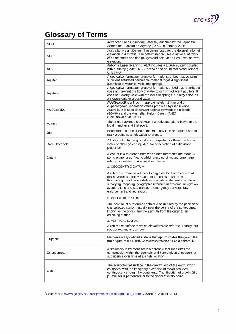
Glossary of Terms ALOS
Advanced Land Observing Satellite, launched by the Japanese Aerospace Exploration Agency (JAXA) in January 2006.
AHD
Australian Height Datum. The datum used for the determination of elevation in Australia. The determination uses a national network of benchmarks and tide gauges and sets Mean Sea Level as zero elevation.
ALS Airborne Laser Scanning. ALS includes a LiDAR system coupled with a survey grade GNSS receiver and an Inertial Measurement Unit (IMU).
Aquifer A geological formation, group of formations, or bed that contains sufficient saturated permeable material to yield significant quantities of water to wells and springs.
Aquitard
A geological formation, group of formations or bed that retards but does not prevent the flow of water to or from adjacent aquifers. It does not readily yield water to wells or springs, but may serve as a storage unit for ground water.
AUSGeoid09
AUSGeoid09 is a 1’ by 1’ (approximately 1.8 km) grid of ellipsoid/geoid separation values produced by Geoscience Australia. It is used to convert heights between the ellipsoid (GDA94) and the Australian Height Datum (AHD). (See Brown et al, 2011)
Azimuth The angle reckoned clockwise in a horizontal plane between the local meridian and that point.
BM Benchmark, a term used to describe any item or feature used to mark a point as an elevation reference.
Bore / borehole A hole sunk into the ground and completed for the extraction of water or other gas or liquid, or for observation of subsurface properties
Datum1
A datum is a reference from which measurements are made. A point, plane, or surface to which systems of measurement are referred or related to one another. Hence:
1. GEOCENTRIC DATUM
A reference frame which has its origin as the Earth's centre of mass, which is directly related to the orbits of satellites. Positioning from these satellites is a critical element in modern surveying, mapping, geographic information systems, navigation, aviation, land and sea transport, emergency services, law enforcement and recreation.
2. GEODETIC DATUM
The position of a reference spheroid as defined by the position of one selected station, usually near the centre of the survey area, known as the origin, and the azimuth from the origin to an adjoining station.
3. VERTICAL DATUM
A reference surface to which elevations are referred, usually, but not always, mean sea level.
Ellipsoid Mathematically-defined surface that approximates the geoid, the truer figure of the Earth. Sometimes referred to as a spheroid.
Extensometer A stationary instrument set in a borehole that measures the compression within the borehole and hence gives a measure of subsidence over time at a single location.
Geoid1
The equipotential surface in the gravity field of the earth, which coincides, with the imaginary extension of mean sea level continuously through the continents. The direction of gravity (the plumbline) is perpendicular to the geoid at every point.
1Source: http://www.ga.gov.au/mapspecs/250k100k/appendix_l.html, Viewed 09 August, 2013.
7
GNSS Global Navigation Satellite Systems. Collective description for all navigation satellite systems including GPS.
GPS Global Positioning System. A constellation of US owned navigation satellites.
GRACE
The Gravity Recovery And Climate Experiment, a joint satellite mission of NASA and the German Aerospace Center, that has been making detailed measurements of Earth's gravity field since its launch in March 2002.
Groundwater2
Groundwater is the water located beneath the earth's surface in soil pore spaces and in the fractures of rock formations.
ICSM Intergovernmental Committee on Surveying and Mapping.
InSAR
Interferometric Synthetic Aperture Radar (InSAR) is a remote sensing technique using two or more synthetic aperture radar (SAR) images to generate maps of surface deformation or elevation.
LiDAR Light Detection and Ranging (LiDAR) is a remote sensing technology that measures distance by illuminating a target with a laser and analysing the reflected light.
MSL Mean Sea Level. The mean level of the sea throughout a definite number of complete tidal cycles.
Orthometric Orthometric height is, for practical purposes, "height above sea level". The current AHD datum is tied to MSL at thirty points around the Australian coast.
PSM Permanent Survey Mark
Photogrammetry The practice of determining the geometric properties of objects from photographic images.
Precise Levelling A particularly accurate method of differential levelling that uses highly accurate levels and adopts a more rigorous observing procedure than general engineering levelling.
Radioactive Bullet Logging
A method to measure compaction and extension of a formation that involves shooting radioactive bullets into a formation at known depths and later surveying the bullets to monitor changes in depth.
RTK
Real Time Kinematic, used to describe a technique of GNSS surveying where observations are transmitted, in real time, from a stationary ‘base’ GNSS receiver to a roving ‘Kinematic’ GNSS receiver for immediate calculation of position.
Spheroid Mathematically-defined surface that approximates the geoid, the truer figure of the Earth, sometimes referred to as an ellipsoid of revolution.
Subsidence
Usually refers to vertical displacement of a point, but the subsidence of the ground actually includes both vertical and horizontal displacements. Subsidence is usually expressed in units of millimetres (mm).
Tilt3
The change in slope of the ground as a result of differential subsidence, and is calculated as a change in subsidence between two points divided by the distance between those points. Tilt is therefore the first derivative of the subsidence profile. Tilt is usually expressed in units of millimetres per metre (mm/m). A tilt of 1mm/m is equivalent to a change in grade of 0.1%.
2 Source: http://en.wikipedia.org/wiki/Groundwater, viewed August 9, 2013.
3 Source: http://www.ukessays.com/essays/environmental-sciences/investigation-of-subsidence-in-the-hunter-region-
environmental-sciences-essay.php, viewed August 9, 2013.

8
1. Introduction
1.1. Objectives and context
The NSW Chief Scientist and Engineer was commissioned to undertake a review of coal seam gas
(CSG) related activities in NSW. The Cooperative Research Centre for Spatial Information were
requested to assist in the production of an information paper on subsidence monitoring, to inform
and develop policy and to assist with public understanding.
The objective of this information paper is to provide a high-level review of the various methods
used nationally and internationally to monitor land subsidence. The paper provides an analysis of
the strengths and weaknesses of the various technologies and methods, particularly with respect to
monitoring subsidence caused by CSG production. This information paper includes a brief review
of measurement and recording of subsidence caused by CSG activities. It investigates the
requirement and approach to developing baseline subsidence measurements to enable an
understanding of ground motion caused by underlying natural and other manmade processes. This
paper also attempts to identify uncertainties, unknowns or research gaps in relation to measuring
and monitoring subsidence related to CSG activities.
1.2. Scope of tasks
This report describes techniques that can be used to monitor subsidence over time.
The scope of tasks encompasses:
Methods that can be used to measure and monitor subsidence, including land-based
surveys, satellite and aerial monitoring and other techniques,
The strengths and weaknesses of the various approaches, with international best practice,
Baseline measurements,
Examples of measurement of subsidence from CSG activities in Australia and overseas,
Availability of on-line subsidence data in NSW regions with CSG activities and
Knowledge gaps and uncertainties.
9
2. Overview of Subsidence Process
The process of CSG extraction involves the removal of groundwater from the coal seam to liberate
methane and other gases that are tightly bound in the matrix of the coal that are of commercial
CSG value. The groundwater is removed by a network of specifically designed CSG wells with their
design largely dependent on the geological and hydrogeological conditions within each field. The
groundwater targeted for extraction within the CSG field is confined to the coal measure rocks at
typical depths of between the range of 300m to 1000m below the surface for most CSG fields in
Australia.
Since extraction takes place at great depth, the groundwater is under pressure and the process of
removal of groundwater from the coal measure rocks changes the overall pressure condition within
the geological sequence. This pressure change is referred to as “depressurisation”. The removal of
groundwater which in-fills the pores and cracks (cleats) within the coal seams results in a reduction
in the “buoyancy” and upward pressures in the coal measure rocks which was previously in
equilibrium with the downward earth pressures from the weight of the overburden sequence of rock
above and within the coal measures. Subsidence can thus occur due to the increase in vertical
stress on the coal sequence rocks being depressurised.
Typical depressurisation in the CSG fields in Australia can be substantial. The hydrostatic pressure
in the coal seams is required to be minimised to roughly 345kPa which correlates to a groundwater
level 35m above the top of the coal seam as part of the depressurisation process (APLNG,
undated, cited in Sydney Catchment Authority, 2012). Although depressurisation changes
groundwater pressure within the coal measures the magnitudes of settlement in theory are small
due to the very high elastic modulus properties (stiffness) of the coal measure rocks.
Currently the only publically available estimates of potential subsidence from CSG extraction in
Australia relate to Queensland developments. Subsidence effects due to aquifer compaction have
been predicted by proponents to be minor (Moran and Vink, 2010). Published estimates from CSG
proponents of absolute subsidence across typical CSG fields in Australia are very small. These
calculated settlements range between 0.08m to 0.18m within fields analysed for recent
developments in S.E Queensland (QGC, 2012). Predicted compaction from these studies is similar
to CSG studies in the western United States (Case, 2000). The resulting settlement (subsidence)
gradients across CSG extraction fields are thus also inferred to be very small, and would generally
not be expected to significantly impact on surface infrastructure. However potential impacts still
need to be confirmed such as for transport infrastructure, streams, pipelines and irrigation lines and
it is for this reason that subsidence monitoring is undertaken.
Current knowledge suggests subsidence induced by dewatering of coal seams is likely to be minor
in comparison to long wall mining. However, small changes to surface topography could change
overland flow patterns and in turn increase erosion (Moran and Vink, 2010).
The timeframe involved in pumping and associated depressurisation varies depending on the CSG
field. Gas production typically becomes significant after a few months of pumping. The rate of
depressurisation in the actual coal seam occurs over months to years. Furthermore the potential for
depressurisation of the underlying and overlying units may take from years to tens of years. The
overall process thus has implications on the time dependency of subsidence and the required
period of monitoring.
10
3. Overview of subsidence monitoring techniques
The following section provides an overview of a range of monitoring techniques used internationally
to measure and monitor surface deformation from subsurface mining and other causes.
Modelling of potential CSG subsidence in Australia indicates that the principle movement will be a
change in height over a broad area caused by depressurisation of the coal seam, and any
horizontal movement is likely to be negligible.
This paper describes a range of standard subsidence monitoring methods and approaches that
provide a direct measure of surface deformation, as well as other technologies that measure
observables that can be related, either directly or indirectly, to surface deformation. Some of the
techniques discussed would require further research and development to confirm suitability for
subsidence monitoring.
The techniques are broadly divided into three groups; surface techniques that involve
measurement directly on the earth’s surface, remote sensing techniques that involve measurement
above the surface and borehole techniques that rely on measurements underneath the surface.
3.1. Surface techniques
Land based survey techniques are typically used in combination with remote sensing or borehole
techniques to provide points of truth against which to check or calibrate the observations and to
provide a known reference frame (coordinate system or datum) for other datasets. Permanent
Survey Marks (PSMs) are placed in positions where they are unlikely to be disturbed or damaged
by processes other than those being monitored (e.g. damaged by a vehicle driving over it). The
term Bench Mark (BM) is used to describe a PSM whose vertical position is known or monitored,
but not its horizontal position, which is known to a lower level of accuracy. Once a network of PSMs
has been established, surveyed and their positions determined they can be re-observed at a later
date to determine the amount of movement, if any, that has occurred. Changes in position of PSMs
provide a measure of movement at discrete locations across a study area.
PSMs are typically spaced at intervals across the study area, with higher density in areas of special
significance. In some circumstances it can be an advantage to survey PSMs along an existing
geophysical (seismic) section line, which allows evaluation of deformation against known
geological structure data. For broad area deformation studies PSMs are often placed within road
reserves or along existing tracks for ease of access. Some PSMs in the network should be located
well outside the area subject to subsidence so that absolute positions, relative to a known datum,
can be determined and maintained between surveys carried out at different times (epochs).
A number of land surface surveying techniques are available to accurately measure position and
change in position over time. These include: precise levelling, high order traversing and Global
Navigation Satellite Systems (GNSS) techniques.
In Australia the ‘Standards and Practices for Control Surveys’ are detailed in the Inter-
governmental Committee on Surveying and Mapping (ICSM) publication of the same name, often
referred to as ‘SP1’, sets out clear standards for accuracy for various control surveys. SP1 (ICSM,
2007) provides recommended survey and reduction practices for vertical and horizontal control
surveys carried out using analogue or digital levels, electronic total stations (electronic theodolites
11
with built in electronic distance measurement) and survey grade Global Navigation Satellite System
(GNSS) receivers. Within Australia, SP1 (ICSM, 2007) is the primary reference document used by
surveyors to determine the most appropriate survey techniques and data reduction practices
required to meet specified accuracy expectations for control surveys.
3.1.1. Precise Levelling
The height of PSMs can be most accurately determined by precise levelling. Precise levelling
measures the differential elevation between sites and adopts a more rigorous observing procedure
than general engineering levelling.
Using precise levelling techniques, accuracies in the order of 1mm over 1km can be achieved.
Precise levelling is typically carried out using a digital level which electronically reads a bar-coded
scale on the staff and includes data recording and reduction capabilities.
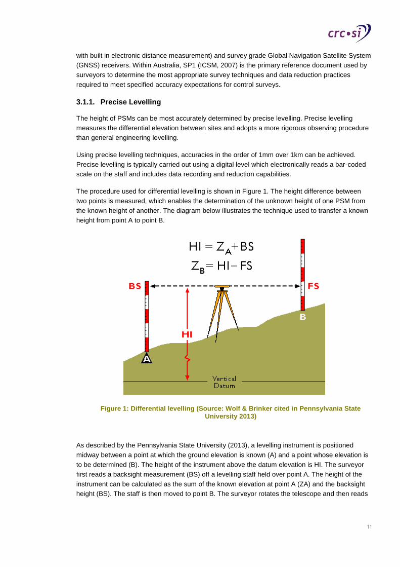
The procedure used for differential levelling is shown in Figure 1. The height difference between
two points is measured, which enables the determination of the unknown height of one PSM from
the known height of another. The diagram below illustrates the technique used to transfer a known
height from point A to point B.
Figure 1: Differential levelling (Source: Wolf & Brinker cited in Pennsylvania State University 2013)
As described by the Pennsylvania State University (2013), a levelling instrument is positioned
midway between a point at which the ground elevation is known (A) and a point whose elevation is
to be determined (B). The height of the instrument above the datum elevation is HI. The surveyor
first reads a backsight measurement (BS) off a levelling staff held over point A. The height of the
instrument can be calculated as the sum of the known elevation at point A (ZA) and the backsight
height (BS). The staff is then moved to point B. The surveyor rotates the telescope and then reads
12
a foresight (FS) off the staff at B. The elevation at B (ZB) can then be calculated as the difference
between the height of the instrument (HI) and the foresight height (FS).
In precise levelling additional factors need to be considered including the curvature of the earth,
which means that a line of sight that is horizontal at the instrument will become higher as distance
increases. The line of sight from the instrument is also affected by refraction in the atmosphere
which, due to the change of air pressure with elevation, causes the line of sight to bend downwards
toward the earth. In precise levelling these errors can be eliminated or minimised by observing at
certain times of the day, minimising sight distances, using equal forward and backsights and
avoiding grazing rays close to the ground. The procedures required to achieve various orders of
accuracy are clearly defined in SP1 (ICSM, 2007).
It should be noted that a properly set up level measures changes in height above the geoid (i.e.
changes in height above mean sea level (MSL)) and not changes in height above the spheroid.
Precise levelling therefore provides orthometric heights consistent with the Australian Height
Datum (AHD), the standard height reference datum used in Australia.
Advantages
Provides very precise height measurement at discrete points. Accuracies in the order of 1mm
over 1km can be achieved.
Disadvantages
Labour intensive, particularly over large areas or in steep terrain;
Only provides heights at discrete points, interpolation required elsewhere.
3.1.2. Control Traverse
The vertical and horizontal coordinates of PSMs can be accurately determined by using a survey
technique known as Traversing, which is used to establish survey control networks. Traversing can
achieve accuracies in the order of 5-10mm over 1km. Traversing is typically carried out using
Electronic Total Station instruments that enable multiple rounds of angles and distances to be
observed and recorded without the need to manually point the instrument or record observations.
Traverse networks involve placing PSMs along a line or path of travel, and then measuring angles
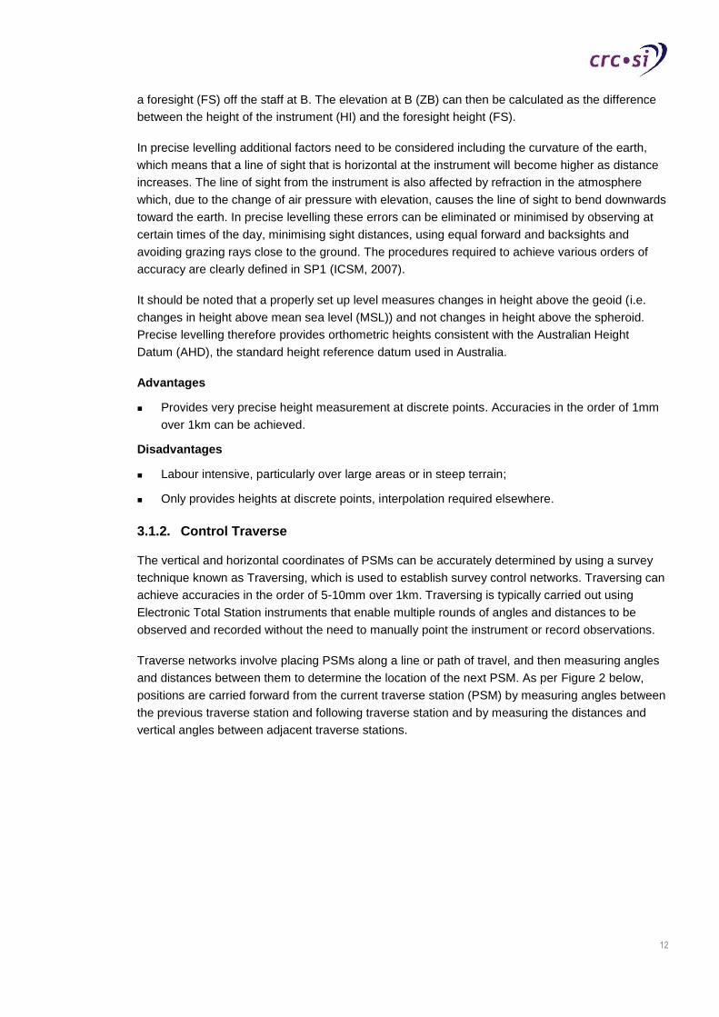
and distances between them to determine the location of the next PSM. As per Figure 2 below,
positions are carried forward from the current traverse station (PSM) by measuring angles between
the previous traverse station and following traverse station and by measuring the distances and
vertical angles between adjacent traverse stations.
13
Figure 2: Principle measurements made in a Traverse (Source: Global Security, 2013)
Traverses start at a known point and require a known azimuth or direction to a second point. To
avoid propagation errors, control traverses are closed against a known pair of PSMs to assure that
observational errors are not carried forward. Closing the traverse enables quantification of any
small errors in distances and angles that may accumulate throughout the traverse. If within
allowable limits, the small errors are distributed throughout the traverse prior to reduction and
calculation of positions for each of the traverse stations (PSMs).
It should be noted that a Total Station observes vertical angles from the zenith defined by a vertical
plumb line. Therefore Traversing, as with Levelling, measures changes in height above the geoid
and therefore provides orthometric heights consistent with the Australian Height Datum (AHD), the
standard height reference datum used in Australia.
High-order traversing techniques include the use of ‘constrained centring’, observing reciprocal
vertical angles and observing multiple distances and rounds of angles at each traverse station. As
with Levelling, the procedures required for various accuracy expectations are clearly defined in
SP1 (ICSM, 2007).
Advantages
Provides very high quality horizontal and vertical measurement at discrete points. Can achieve
accuracies in the order of 5-10mm over 1km
Disadvantages
Labour intensive, particularly over very large areas
Only provides position or change of position at discrete points, interpolation required
elsewhere
3.1.3. GNSS techniques
GNSS is a generic term that refers to all global navigation satellite systems. The most widely
known constellation of navigation satellites is the Global Positioning System (GPS), which refers
specifically to the US navigation satellite system.
14
GNSS ‘survey’ receivers differ significantly from commercially available ‘navigation’ receivers.
Navigation receivers (the type used for bushwalking, boating or in car navigation) rely on signals
broadcast from GNSS satellites to calculate position to an absolute accuracy in the order of 5 to
10m. Encrypted satellite signals can be interpreted by military ‘navigation’ receivers to determine
more accurate position fixes, but even these do not approach the accuracy expectations required
for control surveys.
GNSS ‘survey’ receivers measure the difference in phase between one or more of the carrier
waves transmitted by navigation satellites to derive very accurate three dimensional baselines or
vectors between pairs of GNSS ‘survey’ receivers. Using these carrier wave measurements
baselines between ‘survey’ receivers can be measured to accuracies in the order of 1 part per
million (or 1mm over 1km).
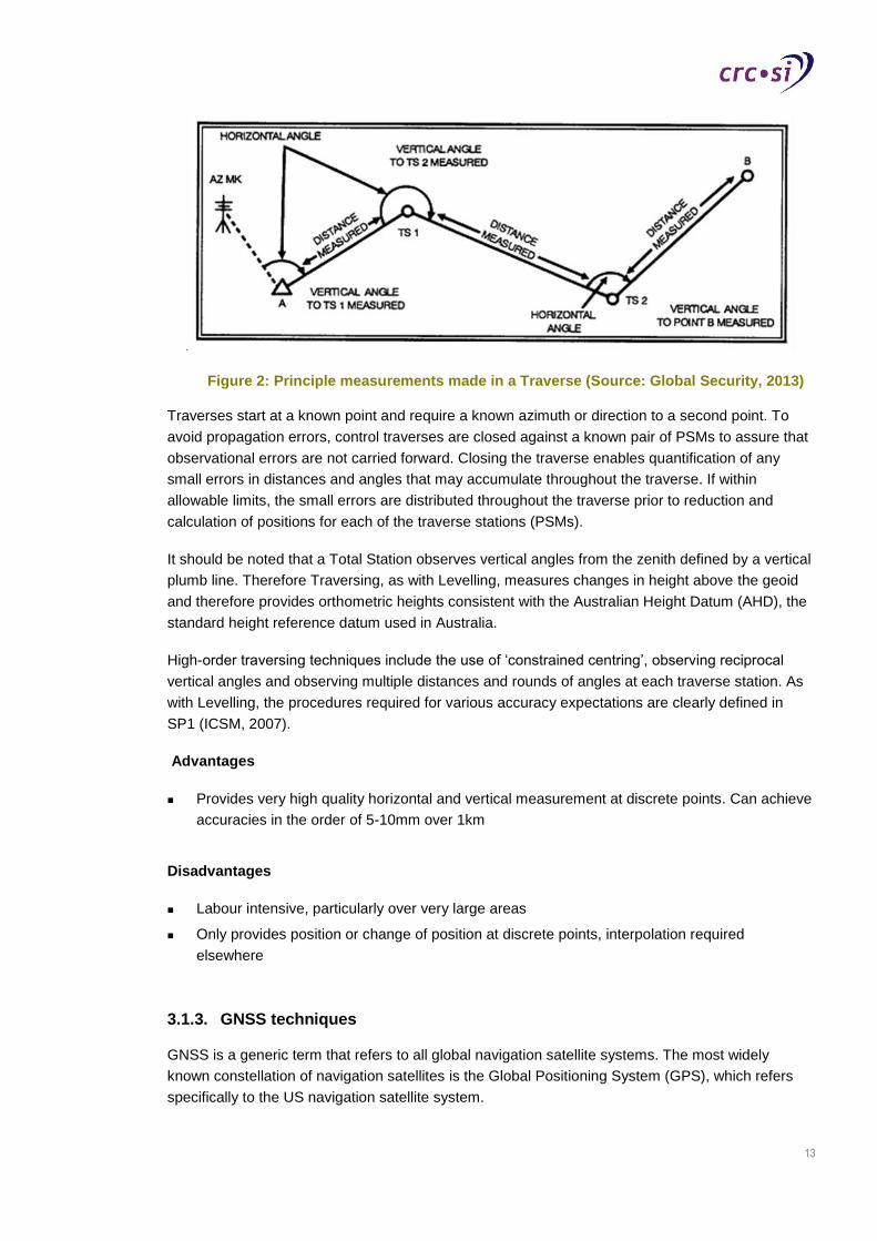
Figure 3: A pair of GPS ‘Survey’ receivers recording carrier phase measurements used to derive an accurate ‘baseline’ between the receivers (Source: ICSM, 2013)
A GNSS baseline is determined by using two survey grade GNSS receivers, one at each end of the
line to be measured (Figure 3). They collect data from the same GNSS satellites at the same
time. The duration of these simultaneous observations may vary with the length of the line and the
accuracy required. The difference in position between the two points is calculated by comparing the
data from both receivers. Many of the uncertainties of GNSS positioning, including satellite and
receiver clock errors, signal delays caused by the atmosphere and uncertainties in satellite
positions are cancelled out or minimised because they are common to observations at each end of
the baseline (ICSM, 2013).
15
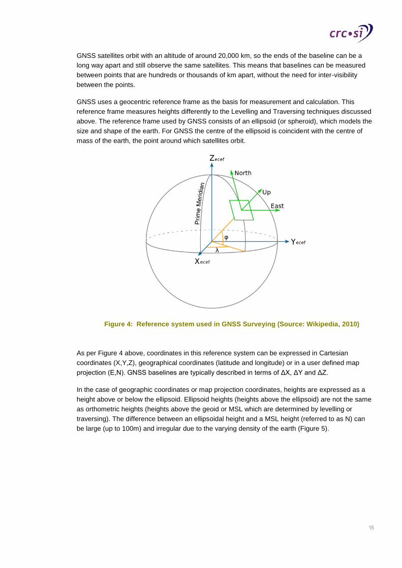
GNSS satellites orbit with an altitude of around 20,000 km, so the ends of the baseline can be a
long way apart and still observe the same satellites. This means that baselines can be measured
between points that are hundreds or thousands of km apart, without the need for inter-visibility
between the points.
GNSS uses a geocentric reference frame as the basis for measurement and calculation. This
reference frame measures heights differently to the Levelling and Traversing techniques discussed
above. The reference frame used by GNSS consists of an ellipsoid (or spheroid), which models the
size and shape of the earth. For GNSS the centre of the ellipsoid is coincident with the centre of
mass of the earth, the point around which satellites orbit.
Figure 4: Reference system used in GNSS Surveying (Source: Wikipedia, 2010)
As per Figure 4 above, coordinates in this reference system can be expressed in Cartesian
coordinates (X,Y,Z), geographical coordinates (latitude and longitude) or in a user defined map
projection (E,N). GNSS baselines are typically described in terms of ΔX, ΔY and ΔZ.
In the case of geographic coordinates or map projection coordinates, heights are expressed as a
height above or below the ellipsoid. Ellipsoid heights (heights above the ellipsoid) are not the same
as orthometric heights (heights above the geoid or MSL which are determined by levelling or
traversing). The difference between an ellipsoidal height and a MSL height (referred to as N) can
be large (up to 100m) and irregular due to the varying density of the earth (Figure 5).
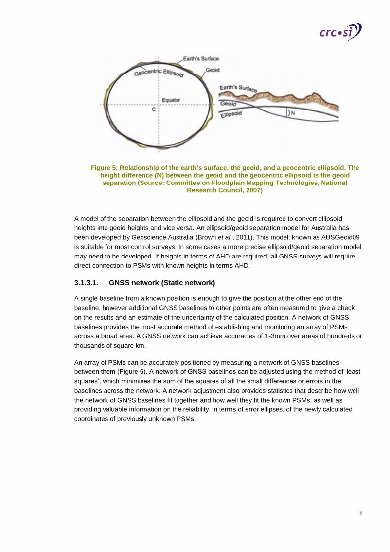
16
Figure 5: Relationship of the earth's surface, the geoid, and a geocentric ellipsoid. The height difference (N) between the geoid and the geocentric ellipsoid is the geoid separation (Source: Committee on Floodplain Mapping Technologies, National
Research Council, 2007)
A model of the separation between the ellipsoid and the geoid is required to convert ellipsoid
heights into geoid heights and vice versa. An ellipsoid/geoid separation model for Australia has
been developed by Geoscience Australia (Brown et al., 2011). This model, known as AUSGeoid09
is suitable for most control surveys. In some cases a more precise ellipsoid/geoid separation model
may need to be developed. If heights in terms of AHD are required, all GNSS surveys will require
direct connection to PSMs with known heights in terms AHD.
3.1.3.1. GNSS network (Static network)
A single baseline from a known position is enough to give the position at the other end of the
baseline, however additional GNSS baselines to other points are often measured to give a check
on the results and an estimate of the uncertainty of the calculated position. A network of GNSS
baselines provides the most accurate method of establishing and monitoring an array of PSMs
across a broad area. A GNSS network can achieve accuracies of 1-3mm over areas of hundreds or
thousands of square km.
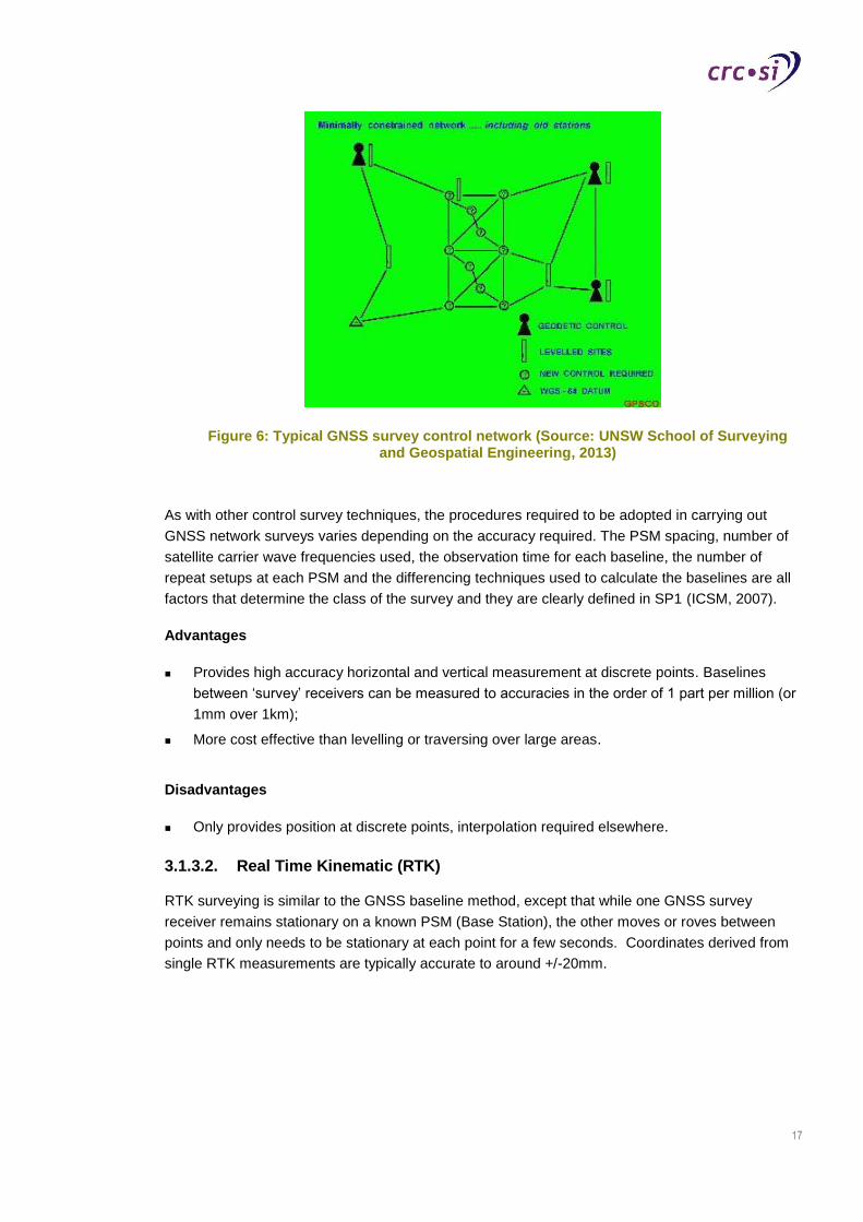
An array of PSMs can be accurately positioned by measuring a network of GNSS baselines
between them (Figure 6). A network of GNSS baselines can be adjusted using the method of ‘least
squares’, which minimises the sum of the squares of all the small differences or errors in the
baselines across the network. A network adjustment also provides statistics that describe how well
the network of GNSS baselines fit together and how well they fit the known PSMs, as well as
providing valuable information on the reliability, in terms of error ellipses, of the newly calculated
coordinates of previously unknown PSMs.
17
Figure 6: Typical GNSS survey control network (Source: UNSW School of Surveying and Geospatial Engineering, 2013)
As with other control survey techniques, the procedures required to be adopted in carrying out
GNSS network surveys varies depending on the accuracy required. The PSM spacing, number of
satellite carrier wave frequencies used, the observation time for each baseline, the number of
repeat setups at each PSM and the differencing techniques used to calculate the baselines are all
factors that determine the class of the survey and they are clearly defined in SP1 (ICSM, 2007).
Advantages
Provides high accuracy horizontal and vertical measurement at discrete points. Baselines
between ‘survey’ receivers can be measured to accuracies in the order of 1 part per million (or
1mm over 1km);
More cost effective than levelling or traversing over large areas.
Disadvantages
Only provides position at discrete points, interpolation required elsewhere.
3.1.3.2. Real Time Kinematic (RTK)
RTK surveying is similar to the GNSS baseline method, except that while one GNSS survey
receiver remains stationary on a known PSM (Base Station), the other moves or roves between
points and only needs to be stationary at each point for a few seconds. Coordinates derived from
single RTK measurements are typically accurate to around +/-20mm.
18
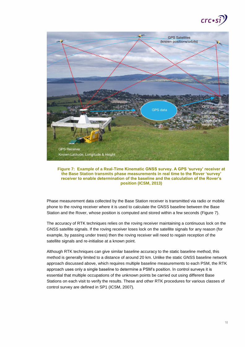
Figure 7: Example of a Real-Time Kinematic GNSS survey. A GPS ‘survey’ receiver at the Base Station transmits phase measurements in real time to the Rover ‘survey’ receiver to enable determination of the baseline and the calculation of the Rover’s
position (ICSM, 2013)
Phase measurement data collected by the Base Station receiver is transmitted via radio or mobile
phone to the roving receiver where it is used to calculate the GNSS baseline between the Base
Station and the Rover, whose position is computed and stored within a few seconds (Figure 7).
The accuracy of RTK techniques relies on the roving receiver maintaining a continuous lock on the
GNSS satellite signals. If the roving receiver loses lock on the satellite signals for any reason (for
example, by passing under trees) then the roving receiver will need to regain reception of the
satellite signals and re-initialise at a known point.
Although RTK techniques can give similar baseline accuracy to the static baseline method, this
method is generally limited to a distance of around 20 km. Unlike the static GNSS baseline network
approach discussed above, which requires multiple baseline measurements to each PSM, the RTK
approach uses only a single baseline to determine a PSM’s position. In control surveys it is
essential that multiple occupations of the unknown points be carried out using different Base
Stations on each visit to verify the results. These and other RTK procedures for various classes of
control survey are defined in SP1 (ICSM, 2007).
19
Advantages
Provides high accuracy horizontal and vertical measurement at discrete points. Coordinates
derived from single RTK measurements are typically accurate to around +/-20mm;
Can be more cost effective than a GNSS network survey in clear areas within broadcast range
of a base station.
Disadvantages
Limited to approximately 20km from base station;
Less accurate than GNSS baseline network survey;
Only provides position at discrete points, interpolation required elsewhere;
Impractical in some areas if roving receiver cannot maintain lock (e.g. due to heavy vegetation
or tall buildings).
3.1.4. Tiltmeters
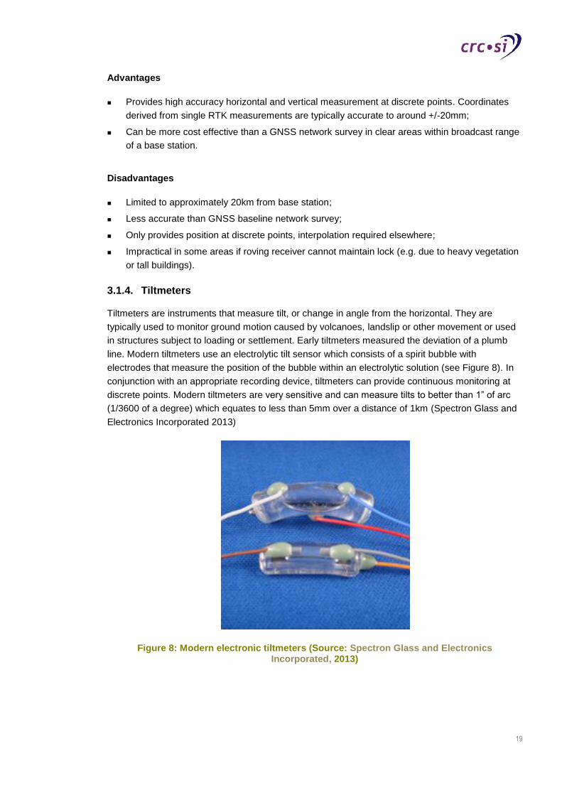
Tiltmeters are instruments that measure tilt, or change in angle from the horizontal. They are
typically used to monitor ground motion caused by volcanoes, landslip or other movement or used
in structures subject to loading or settlement. Early tiltmeters measured the deviation of a plumb
line. Modern tiltmeters use an electrolytic tilt sensor which consists of a spirit bubble with
electrodes that measure the position of the bubble within an electrolytic solution (see Figure 8). In
conjunction with an appropriate recording device, tiltmeters can provide continuous monitoring at
discrete points. Modern tiltmeters are very sensitive and can measure tilts to better than 1” of arc
(1/3600 of a degree) which equates to less than 5mm over a distance of 1km (Spectron Glass and
Electronics Incorporated 2013)
Figure 8: Modern electronic tiltmeters (Source: Spectron Glass and Electronics Incorporated, 2013)
20
Advantages
Provide near-continuous tilt measurements at discrete points. Can measure tilts to better than
1” of arc (1/3600 of a degree) which equates to less than 5mm over a distance of 1km.
Disadvantages
Provides change in tilt measurement only, does not provide a change in position.
3.1.5. Microgravity Survey
Gravity varies with the distance from the Earth’s centre of mass and with changes in subsurface
density. The distance of a point from the Earth’s centre of mass can be directly related to its
elevation, therefore microgravity measurements can be used to monitor changes in height (due to
subsidence) and changes in surface density (due to fluid extraction). Gravity can be measured to
an accuracy that equates to changes in height of around 1 to 2cm.
Undertaking a microgravity survey involves the collection of sensitive gravity measurements on the
ground surface at discrete points. Changes in gravity are referred to as gravity anomalies and are
normally interpreted to reveal subsurface variations in density (Telford et al., and Seigel et al., cited
in Benson, et al., 2003).
Microgravity surveys have been used for decades in oil and mineral exploration. Advances in
microgravity equipment have improved the accuracy and efficiency of obtaining microgravity data
and have extended the application of the method to geotechnical and environmental site
characterisations (Kaufmann and Doll, cited in Benson et al., 2003).
The United States Geological Survey (USGS) Arizona Water Science Centre has used microgravity
for groundwater monitoring, as aquifer storage increases after heavy rain and decreases with
groundwater pumping and natural discharge. Repeat microgravity measurements over time
showing increases in gravity indicate an increase in groundwater storage due to the extra mass in
the subsurface, whereas decreasing gravity over time indicates a decrease in storage. Gravity
studies between 1999 and 2002 in the Tucson Valley in Arizona show the largest decrease in
gravity in areas where local groundwater providers extract ground water and increase where water
is actively recharged (O'Rear, 2011).
Microgravity surveys may be able to be used to monitor the effects of CSG production on the
environment. Given that microgravity readings are linked to both height and ground water storage
volumes and that reduction in ground water storage volumes is directly related to surface
subsidence, it follows that gravity surveys may provide an alternative method to monitor
subsidence and groundwater extraction.
The microgravity method could potentially be used to monitor CSG activities but would probably
require further scientific investigation and detailed modelling to separate the effects of subsidence
and water extraction.
21
Advantages
Relatively easy to measure;
Gravity can be measured to an accuracy that equates to changes in height of around 1 to 2cm.
Disadvantages
Does not measure deformation directly;
Responds to both subsidence and water extraction;
Only provides measurements at discrete points, interpolation required elsewhere.
3.2. Remote sensing techniques
Remote sensing involves the acquisition of information using sensors mounted on a satellite or
aircraft platform. Unlike ground surveys that are limited to monitoring specific locations that rely on
interpolation of surface change in areas away from the monitoring points, remote sensing
techniques can measure surface movement for specific locations and over broad areas.
Repeat surveys allow for the monitoring of changes in relative or absolute subsidence over time.
Most remote sensing techniques rely to some extent on ground survey data to provide control or
calibration of the data.
3.2.1. Interferometric Synthetic Aperture Radar (InSAR)
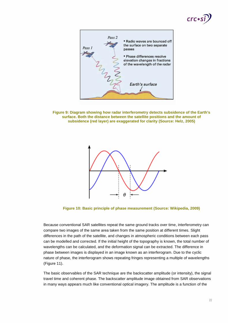
Interferometric synthetic aperture radar, abbreviated InSAR, is a satellite-based remote sensing
technique that uses radar signals to measure changes in land surface elevation over time (Figure
9). InSAR has been demonstrated as a cost-effective solution to measuring land surface
deformation on a regional scale with a high degree of spatial detail and resolution. In ideal
measurement conditions InSAR can measure ground surface subsidence or uplift at the sub-
centimetre level. The technique has been successfully demonstrated in Australia and
internationally for monitoring: subsidence from underground long wall mining (Chang et al., 2007a,
2007b); earthquake studies with a measurement capability of better than 3 mm (Cummins et al.
2008), and aquifer response to groundwater pumping (Amelung et al., 2008).
Interferometry measures small differences in phase between the transmitted radar signal and the
reflected radiation from the Earth’s surface. The phase of the outgoing wave is compared to the
phase of the return signal, which depends on the distance to the ground. This is observable as a
phase difference or phase shift in the returning wave. Although the total distance to the satellite
(i.e., the number of whole wavelengths) is not known to the same level of precision, the extra
fraction of a wavelength can be measured extremely accurately (Figure 10) by calculating the
relative distance changes between pixels over the imaged areas. By adopting reference pixels
outside the area of deformation, or alternatively by using GPS for control, highly precise relative
measurements of subsidence can be determined.
22
Figure 9: Diagram showing how radar interferometry detects subsidence of the Earth's surface. Both the distance between the satellite positions and the amount of
subsidence (red layer) are exaggerated for clarity (Source: Helz, 2005)
Figure 10: Basic principle of phase measurement (Source: Wikipedia, 2009)
Because conventional SAR satellites repeat the same ground tracks over time, interferometry can
compare two images of the same area taken from the same position at different times. Slight
differences in the path of the satellite, and changes in atmospheric conditions between each pass
can be modelled and corrected. If the initial height of the topography is known, the total number of
wavelengths can be calculated, and the deformation signal can be extracted. The difference in
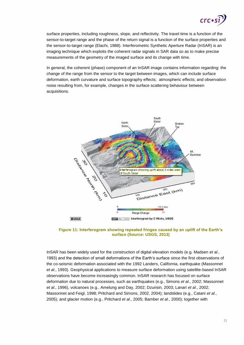
phase between images is displayed in an image known as an interferogram. Due to the cyclic
nature of phase, the interferogram shows repeating fringes representing a multiple of wavelengths
(Figure 11).
The basic observables of the SAR technique are the backscatter amplitude (or intensity), the signal
travel time and coherent phase. The backscatter amplitude image obtained from SAR observations
in many ways appears much like conventional optical imagery. The amplitude is a function of the
23
surface properties, including roughness, slope, and reflectivity. The travel time is a function of the
sensor-to-target range and the phase of the return signal is a function of the surface properties and
the sensor-to-target range (Elachi, 1988). Interferometric Synthetic Aperture Radar (InSAR) is an
imaging technique which exploits the coherent radar signals in SAR data so as to make precise
measurements of the geometry of the imaged surface and its change with time.
In general, the coherent (phase) component of an InSAR image contains information regarding: the
change of the range from the sensor to the target between images, which can include surface
deformation, earth curvature and surface topography effects; atmospheric effects; and observation
noise resulting from, for example, changes in the surface scattering behaviour between
acquisitions.
Figure 11: Interferogram showing repeated fringes caused by an uplift of the Earth’s surface (Source: USGS, 2013)
InSAR has been widely used for the construction of digital elevation models (e.g. Madsen et al.,
1993) and the detection of small deformations of the Earth’s surface since the first observations of
the co-seismic deformation associated with the 1992 Landers, California, earthquake (Massonnet
et al., 1993). Geophysical applications to measure surface deformation using satellite-based InSAR
observations have become increasingly common. InSAR research has focused on surface
deformation due to natural processes, such as earthquakes (e.g., Simons et al., 2002; Massonnet
et al., 1996), volcanoes (e.g., Amelung and Day, 2002; Dzurisin, 2003; Lanari et al., 2002;
Massonnet and Feigl, 1998; Pritchard and Simons, 2002, 2004); landslides (e.g., Catani et al.,
2005); and glacier motion (e.g., Pritchard et al., 2005; Bamber et al., 2000); together with
24
anthropogenic processes, such as subsidence caused by groundwater extraction (e.g., Bawden et
al., 2001; Hoffmann et al., 2001) and mining activity (e.g., Raucoules et al., 2003).
Limitations of the InSAR technique associated with decorrelation and un-modelled atmospheric
signal can be in part mitigated by temporal analysis techniques where many SAR acquisitions are
combined in a single analysis. There are many published temporal analysis techniques including
simple image stacking, persistent scatterers InSAR, and the Small BAseline Subset (SBAS)
techniques.
High resolution InSAR satellites need to be specifically tasked to acquire data over an area of
interest. Other InSAR satellites, like the now inoperable ALOS satellite, have generated an archive
of data over broad areas. Access to archived InSAR data provides the opportunity to map
deformation over areas of interest for a period time prior to CSG production, thus providing the
opportunity to assess deformation caused by natural and manmade causes other than CSG
production. More detailed on-going monitoring can then be carried through the acquisition and
analysis of high resolution InSAR data specifically tasked to cover the area of interest.
Advantages
Provide broad area measurement at horizontal resolutions of 2m to 100m depending on the
sensor system used;
Provide the opportunity to model ground deformation over a period prior to CSG production;
Under favourable conditions, accuracies of 5mm to 10mm are possible in the line of sight of
the radar;
Cost effective for measuring subsidence on a regional scale (Galloway 2000);
Can acquire InSAR data through clouds in the sky.
Disadvantages
Accuracy is dependent on vegetation, topography, the sensor, image processing methods and
the atmospheric conditions when the measurements were acquired (Amelung et al., 2006);
More effective for determining subsidence in urban than rural areas;
Measures change in height between epochs, needs ground control to determine absolute
heights.
3.2.2. Stereo photogrammetry
Photogrammetry is the practice of determining the geometric properties of objects from
photographic images. Photogrammetry is a passive form of remote sensing and relies on the
ambient visible or infrared light reflected from the surface. Unlike InSAR, aerial photography relies
on a clear view of the ground and cannot be acquired through cloud.
Satellite imagery would not provide the resolution or accuracy required for the measurement of the
relatively small levels of deformation expected from CSG production. Photogrammetric techniques
using high resolution, large scale photography enables absolute accuracies in the order of +/-
50mm to be achieved for points on clear, well defined features.
25
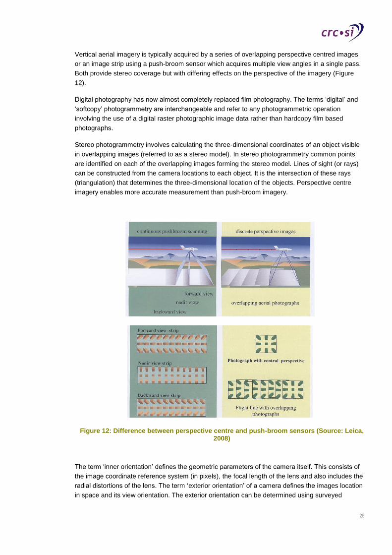
Vertical aerial imagery is typically acquired by a series of overlapping perspective centred images
or an image strip using a push-broom sensor which acquires multiple view angles in a single pass.
Both provide stereo coverage but with differing effects on the perspective of the imagery (Figure
12).
Digital photography has now almost completely replaced film photography. The terms ‘digital’ and
‘softcopy’ photogrammetry are interchangeable and refer to any photogrammetric operation
involving the use of a digital raster photographic image data rather than hardcopy film based
photographs.
Stereo photogrammetry involves calculating the three-dimensional coordinates of an object visible
in overlapping images (referred to as a stereo model). In stereo photogrammetry common points
are identified on each of the overlapping images forming the stereo model. Lines of sight (or rays)
can be constructed from the camera locations to each object. It is the intersection of these rays
(triangulation) that determines the three-dimensional location of the objects. Perspective centre
imagery enables more accurate measurement than push-broom imagery.
Figure 12: Difference between perspective centre and push-broom sensors (Source: Leica, 2008)
The term ‘inner orientation’ defines the geometric parameters of the camera itself. This consists of
the image coordinate reference system (in pixels), the focal length of the lens and also includes the
radial distortions of the lens. The term ‘exterior orientation’ of a camera defines the images location
in space and its view orientation. The exterior orientation can be determined using surveyed
26
ground coordinates of features visible in the imagery, known as Ground Control Points (GCPs).
Once the ‘interior’ and ‘exterior’ orientations are known for both images, forming a stereo model,
the positions of all other features in the model can be determined and measured in real world
coordinates.
Various methods have been devised to eliminate or reduce the requirement for GCPs in every
model. These include using common image tie points to determine the relative orientation of
multiple models within a block of images. A process called aero-triangulation uses this approach to
significantly reduce the number of GCPs required. The use of inertial measurement systems on
board the aircraft reduces the requirement for ground control still further.
The accuracy of photogrammetry is determined by the resolution and focal length of the camera
system, the flying height and methods used. High resolution photography acquired at low level
provides the highest accuracy but the trade-off is cost because the lower the photography is flown
the more frames are required to cover a given area.
Advantages
Provides broad area measurement;
Using low level photography vertical accuracies in the order of 50mm are possible.
Disadvantages
High accuracy photogrammetry is not cost effective over very large areas.
3.2.3. Airborne LiDAR
Light Detection and Ranging (LiDAR) is a remote sensing technology that measures distance by
illuminating a target with a laser and analysing the reflected light. The term airborne LiDAR involves
using a LiDAR system in a moving aircraft and is often referred to as Airborne Laser Scanning
(ALS). ALS has become a technology of choice for the acquisition of digital terrain or surface data
over broad areas. LiDAR surveys can achieve a vertical accuracy of around 10 to 15cm following
Australian LiDAR Acquisition Standards published by ICSM (2011).
ALS incorporates a LiDAR system with a survey grade GNSS receiver and an Inertial
Measurement Unit (IMU), which determines the absolute position and orientation of the sensor, and
a computer to control the system and store data. The laser scanner uses an oscillating mirror or
rotating prism, so that the light pulses sweep across a swath of landscape below the aircraft
(Figure 13). Large areas are surveyed with a series of overlapping parallel flight lines. The laser
pulses used are eye safe and flights can be carried out day or night, as long as the skies are clear.
LiDAR systems can measure over 100,000 pulses every second and have the capability of
measuring multiple points per square metre on the ground (typically between 1 and 40). The laser
footprint varies from around 10cm up to 1m. The footprint size and the number of points measured
per square metre are a function of the LiDAR system used, the flying height and speed of the
aircraft.
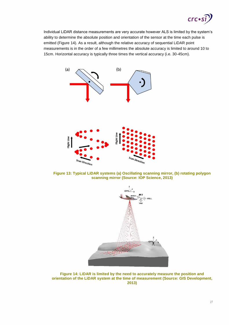
27
Individual LiDAR distance measurements are very accurate however ALS is limited by the system’s
ability to determine the absolute position and orientation of the sensor at the time each pulse is
emitted (Figure 14). As a result, although the relative accuracy of sequential LiDAR point
measurements is in the order of a few millimetres the absolute accuracy is limited to around 10 to
15cm. Horizontal accuracy is typically three times the vertical accuracy (i.e. 30-45cm).
Figure 13: Typical LiDAR systems (a) Oscillating scanning mirror, (b) rotating polygon scanning mirror (Source: IOP Science, 2013)
Figure 14: LiDAR is limited by the need to accurately measure the position and orientation of the LiDAR system at the time of measurement (Source: GIS Development,
2013)
28
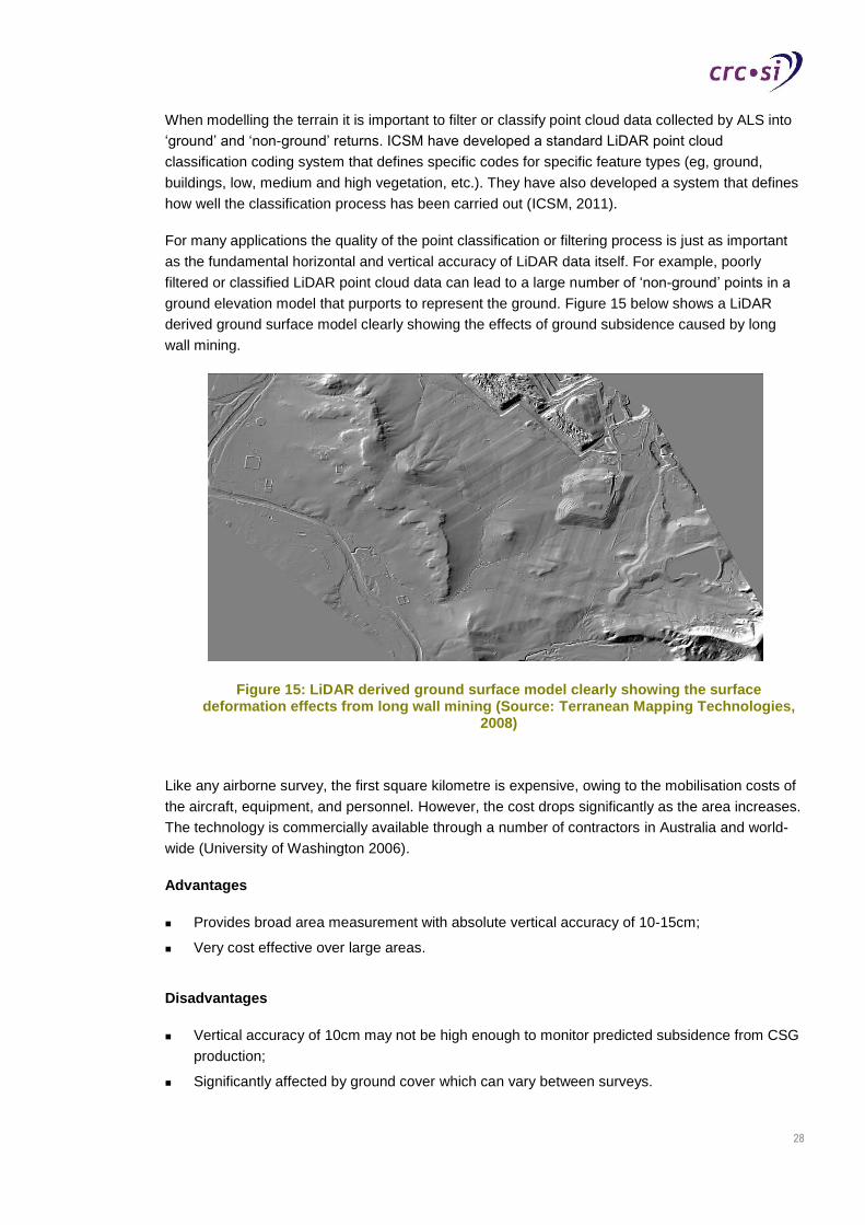
When modelling the terrain it is important to filter or classify point cloud data collected by ALS into
‘ground’ and ‘non-ground’ returns. ICSM have developed a standard LiDAR point cloud
classification coding system that defines specific codes for specific feature types (eg, ground,
buildings, low, medium and high vegetation, etc.). They have also developed a system that defines
how well the classification process has been carried out (ICSM, 2011).
For many applications the quality of the point classification or filtering process is just as important
as the fundamental horizontal and vertical accuracy of LiDAR data itself. For example, poorly
filtered or classified LiDAR point cloud data can lead to a large number of ‘non-ground’ points in a
ground elevation model that purports to represent the ground. Figure 15 below shows a LiDAR
derived ground surface model clearly showing the effects of ground subsidence caused by long
wall mining.
Figure 15: LiDAR derived ground surface model clearly showing the surface deformation effects from long wall mining (Source: Terranean Mapping Technologies,
2008)
Like any airborne survey, the first square kilometre is expensive, owing to the mobilisation costs of
the aircraft, equipment, and personnel. However, the cost drops significantly as the area increases.
The technology is commercially available through a number of contractors in Australia and world-
wide (University of Washington 2006).
Advantages
Provides broad area measurement with absolute vertical accuracy of 10-15cm;
Very cost effective over large areas.
Disadvantages
Vertical accuracy of 10cm may not be high enough to monitor predicted subsidence from CSG
production;
Significantly affected by ground cover which can vary between surveys.
29
3.2.4. Gravity Recovery and Climate Change Experiment (GRACE)
The GRACE satellite system maps the earth's gravity field by making accurate measurements of
the distance between the two satellites using GPS and a microwave ranging system. GRACE has
been used to map the Earth's gravity field with unprecedented accuracy, yielding crucial
information about the distribution and flow of mass within the Earth and its surroundings and
improving the understanding about the Earth's natural systems (NASA 2013).
Gravity changes as a response to the changes in mass of water on or beneath the surface.
Satellite mapping of gravity using GRACE, along with measurements on the ground, could help us
understand more about the effects of water movement caused by CSG production and could be
linked to land subsidence. The use of gravity data collected from GRACE, together with ground
data associated with CSG activities could be the subject of further scientific investigation to
determine if GRACE gravity data can be used to monitor the effects of CSG production on the
environment.
Advantages
Can detect changes in the Earth’s gravity over time over large areas.
Disadvantages
Changes in the Earth’s gravity can be caused by both subsidence and water withdrawal;
Does not measure deformation directly;
May not have a direct, observable link to deformation.
3.3. Borehole techniques
There are a number of monitoring techniques which measure the compression or expansion of
material through which a borehole has been drilled. These systems measure the change in
distance over time from the bottom to the top of the borehole or from a number of locations within
the borehole.
3.3.1. Extensometer
A borehole extensometer measures the changes in longitudinal displacement over time along the
length of a borehole. Borehole extensometers typically consist of a vertical borehole lined with a
tube around 10cm in diameter. A wire or thin rod, anchored at the base of the borehole, passes
through the tube to the surface. Changes in surface height relative to the base of the borehole can
be measured as a change in the length of the wire or rod. These changes are typically recorded by
a measuring device on the surface. Extensometers have been used to measure the deformation
between bottom of a borehole and surface with a vertical accuracy of 3mm (Reed and Yuill, 2009).
Extensometers allow the detailed measurement of subsidence at a specific location. With a suitable
recording device the measurements can be continuous throughout the period of instrumentation.
30
Multiple extensometers are required to monitor the cumulative impacts from multiple pumping
bores over a broad area.
Advantages
Subsidence measurements can be made at a specific location to an accuracy of around 3mm;
Extensometers can measure continuously throughout the period of instrumentation.
Disadvantages
Multiple extensometers are required to measure subsidence over broad areas;
Extensometers only measure deformation between the bottom and the top of the borehole.
3.3.2. Radioactive bullet logging
Radioactive bullet logging involves shooting radioactive bullets into the walls of boreholes. Each
bullet contains a long lived, but low strength, radioactive source. The relative depths of the
radioactive bullets are later measured using a gamma ray probe which is lowered down the
borehole.
Measurement error is in the order of 1cm over 100m. Logging time of around one hour for each 20
m of borehole is required for measurements (Poland et al., 1984).
Advantages
Subsidence measurements can be achieved for a point source of subsidence, such as near a
pumping bore to an accuracy of around 1cm over 100m;.
Can measure differential compression throughout the borehole
Disadvantages
Logging can be time consuming
Accuracy limitations may not detect predicted levels of subsidence from CSG production
3.3.3. Casing-collar logging
Similar to radioactive bullet logging but uses magnetic collars anchored to the geological strata
within the borehole. The positions of the collars are later resurveyed by a magnetic detector passed
down the borehole, and any change in position is used to measure compaction or expansion.
Advantages
Subsidence measurements can be achieved for a point source of subsidence, such as near a
pumping bore.

31
Can measure differential compression throughout the borehole
Disadvantages
Logging can be time consuming
Accuracy limitations my not detect predicted levels of subsidence from CSG production.
32
4. Comparative analysis of monitoring options
A comparative analysis of the various deformation monitoring options discussed in the previous
section has been carried out with particular consideration to their suitability to monitoring the levels
of subsidence likely to be associated with CSG production.
Current published estimates of potential subsidence gradients across Australian CSG extraction
fields range from 0.08-0.18m (QGC, 2012). While this is significantly less than subsidence induced
by long wall mining (Sydney Catchment Authority, 2012), CSG fields may cover the entire aerial
extent of an underground coal seam and hence may extend over hundreds (or thousands) of
square kilometres. The subsidence from CSG production maybe small enough to fall within the
natural variability of landscape processes, but local effects may arise if depressurisation of aquifers
causes some dewatering of unconsolidated alluvial deposits at the surface.
Techniques suitable for monitoring deformation from CSG therefore must be capable of measuring
small changes in height, in the order 1-2cm, over very large areas (hundreds to thousands of
square kilometres) and over relatively long time frames of 10 or more years.
The assessment approach includes, for each option, a review of:
the measurement observable (e.g. change in height, position, tilt, gravity, etc),
the accuracy of the measurement observable,
the advantage and disadvantages of the technique and
a relative comparison of the
accuracy,
suitability for monitoring large areas,
relative cost and
overall suitability for monitoring deformation from CSG production.
33
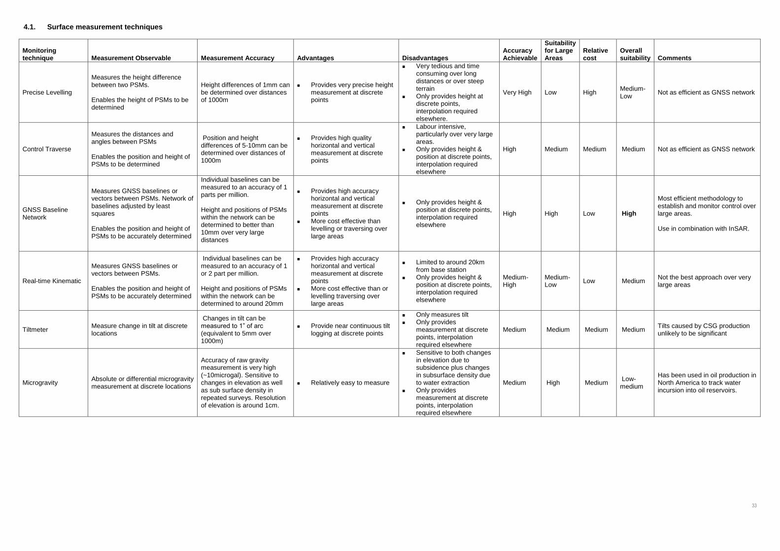
4.1. Surface measurement techniques
Monitoring technique Measurement Observable Measurement Accuracy Advantages Disadvantages
Accuracy Achievable
Suitability for Large Areas
Relative cost
Overall suitability Comments
Precise Levelling
Measures the height difference between two PSMs. Enables the height of PSMs to be determined
Height differences of 1mm can be determined over distances of 1000m
Provides very precise height measurement at discrete points
Very tedious and time consuming over long distances or over steep terrain
Only provides height at discrete points, interpolation required elsewhere.
Very High Low High Medium-Low
Not as efficient as GNSS network
Control Traverse
Measures the distances and angles between PSMs Enables the position and height of PSMs to be determined
Position and height differences of 5-10mm can be determined over distances of 1000m
Provides high quality horizontal and vertical measurement at discrete points
Labour intensive, particularly over very large areas.
Only provides height & position at discrete points, interpolation required elsewhere
High Medium Medium Medium Not as efficient as GNSS network
GNSS Baseline Network
Measures GNSS baselines or vectors between PSMs. Network of baselines adjusted by least squares Enables the position and height of PSMs to be accurately determined
Individual baselines can be measured to an accuracy of 1 parts per million. Height and positions of PSMs within the network can be determined to better than 10mm over very large distances
Provides high accuracy horizontal and vertical measurement at discrete points
More cost effective than levelling or traversing over large areas
Only provides height & position at discrete points, interpolation required elsewhere
High High Low High
Most efficient methodology to establish and monitor control over large areas. Use in combination with InSAR.
Real-time Kinematic
Measures GNSS baselines or vectors between PSMs. Enables the position and height of PSMs to be accurately determined
Individual baselines can be measured to an accuracy of 1 or 2 part per million. Height and positions of PSMs within the network can be determined to around 20mm
Provides high accuracy horizontal and vertical measurement at discrete points
More cost effective than or levelling traversing over large areas
Limited to around 20km from base station
Only provides height & position at discrete points, interpolation required elsewhere
Medium-High
Medium-Low
Low Medium Not the best approach over very large areas
Tiltmeter Measure change in tilt at discrete locations
Changes in tilt can be measured to 1” of arc (equivalent to 5mm over 1000m)
Provide near continuous tilt logging at discrete points
Only measures tilt Only provides
measurement at discrete points, interpolation required elsewhere
Medium Medium Medium Medium Tilts caused by CSG production unlikely to be significant
Microgravity Absolute or differential microgravity measurement at discrete locations
Accuracy of raw gravity measurement is very high (~10microgal). Sensitive to changes in elevation as well as sub surface density in repeated surveys. Resolution of elevation is around 1cm.
Relatively easy to measure
Sensitive to both changes in elevation due to subsidence plus changes in subsurface density due to water extraction
Only provides measurement at discrete points, interpolation required elsewhere
Medium High Medium Low-medium
Has been used in oil production in North America to track water incursion into oil reservoirs.
34
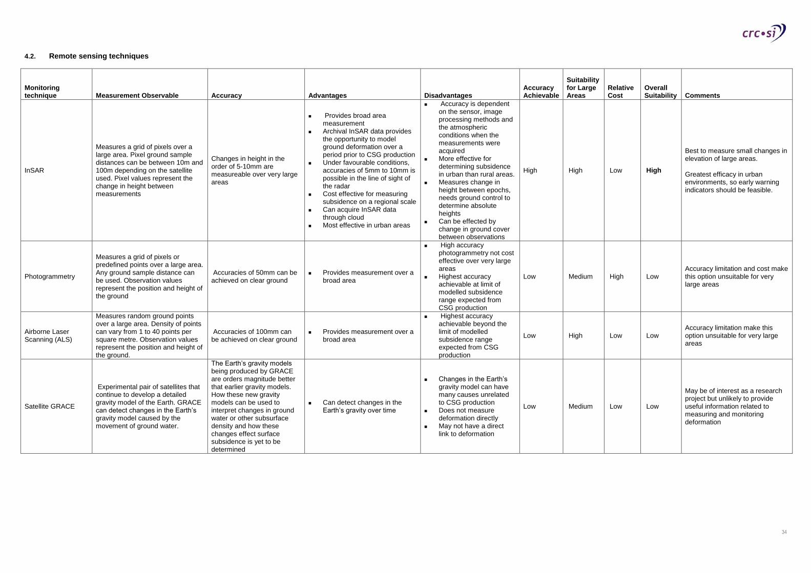
4.2. Remote sensing techniques
Monitoring technique Measurement Observable Accuracy Advantages Disadvantages
Accuracy Achievable
Suitability for Large Areas
Relative Cost
Overall Suitability Comments
InSAR
Measures a grid of pixels over a large area. Pixel ground sample distances can be between 10m and 100m depending on the satellite used. Pixel values represent the change in height between measurements
Changes in height in the order of 5-10mm are measureable over very large areas
Provides broad area measurement
Archival InSAR data provides the opportunity to model ground deformation over a period prior to CSG production
Under favourable conditions, accuracies of 5mm to 10mm is possible in the line of sight of the radar
Cost effective for measuring subsidence on a regional scale
Can acquire InSAR data through cloud
Most effective in urban areas
Accuracy is dependent on the sensor, image processing methods and the atmospheric conditions when the measurements were acquired
More effective for determining subsidence in urban than rural areas.
Measures change in height between epochs, needs ground control to determine absolute heights
Can be effected by change in ground cover between observations
High High Low High
Best to measure small changes in elevation of large areas. Greatest efficacy in urban environments, so early warning indicators should be feasible.
Photogrammetry
Measures a grid of pixels or predefined points over a large area. Any ground sample distance can be used. Observation values represent the position and height of the ground
Accuracies of 50mm can be achieved on clear ground
Provides measurement over a broad area
High accuracy photogrammetry not cost effective over very large areas
Highest accuracy achievable at limit of modelled subsidence range expected from CSG production
Low Medium High Low Accuracy limitation and cost make this option unsuitable for very large areas
Airborne Laser Scanning (ALS)
Measures random ground points over a large area. Density of points can vary from 1 to 40 points per square metre. Observation values represent the position and height of the ground.
Accuracies of 100mm can be achieved on clear ground
Provides measurement over a broad area
Highest accuracy achievable beyond the limit of modelled subsidence range expected from CSG production
Low High Low Low Accuracy limitation make this option unsuitable for very large areas
Satellite GRACE
Experimental pair of satellites that continue to develop a detailed gravity model of the Earth. GRACE can detect changes in the Earth’s gravity model caused by the movement of ground water.
The Earth’s gravity models being produced by GRACE are orders magnitude better that earlier gravity models. How these new gravity models can be used to interpret changes in ground water or other subsurface density and how these changes effect surface subsidence is yet to be determined
Can detect changes in the Earth’s gravity over time
Changes in the Earth’s gravity model can have many causes unrelated to CSG production
Does not measure deformation directly
May not have a direct link to deformation
Low Medium Low Low
May be of interest as a research project but unlikely to provide useful information related to measuring and monitoring deformation

35
4.3. Borehole techniques
Monitoring technique Measurement Observable Accuracy Advantages Disadvantages
Accuracy Achievable
Suitability for Large Areas
Relative Cost
Overall Suitability Comments
Extensometer
Direct measurement of deformation by monitoring the difference in height from the bottom of a borehole to the surface.
1-3mm over the depth of the borehole.
Extensometers can continually measure and log subsidence
Expensive to install Only measure
deformation between the bottom and the top of the borehole
Only provides measurement at discrete points, interpolation required elsewhere
High Low- Medium
High Low-Medium
May be useful in helping develop a greater understanding of how to model CSG subsidence
Radioactive Bullet logging
Indirect measurement of column deformation by monitoring the difference in height from the surface to radioactive bullets fired into the formation at known depths.
Around 1cm over 100m Can measure differential
subsidence throughout the length of the borehole
Expensive to install Only provides
measurement at discrete points, interpolation
Medium Low High Low
May have some relevance in helping develop a greater understanding of how to model CSG subsidence
Casing collar logging
Indirect measurement of column deformation by monitoring the difference in height from the surface to magnetic casing collars in the borehole
Around 30mm between collars
Can measure differential subsidence throughout the length of the borehole
Expensive to install Only provides
measurement at discrete points, interpolation required elsewhere
Low Low High Low Limited accuracy
36
5. Review of CSG monitoring activities
5.1. National CSG Monitoring Activities
Due to only the recent emergence of the industry, there are no long baseline studies, however,
there are currently four CSG proponents in Queensland collaborating to commission a regional
InSAR study of historical and current earth surface movements, to provide certainty for regulatory
and public concerns (Dawson et al., 2011).
The Queensland Government has recently installed a bore line in the Condamine Alluvium that will
be used to monitor subsidence on a transect across the alluvium on an on-going basis (Moran and
Vink 2010).
The Federal Government, through Geoscience Australia has started to establish the Australian
Geophysical Observing Network (AGON). AGON infrastructure will include a network of radar
corner reflectors (clearly visible in InSAR images) and a geodetic network for monitoring ground
deformation in Australia (Dawson et al., 2011).
The geodetic network of PSMs will be coordinated and monitored using a GNSS network. The
radar corner cube reflectors placed in the Surat Basin in Queensland will be linked into the GNSS
network to provide a direct link between InSAR measurements and the GNSS network. This
combination of precise remote sensing and targeted ground measurements represent the current
best practice to determine the impacts of CSG extraction on land subsidence (Dawson et al.,
2011).
Limited numerical modelling of the potential maximum subsidence across CSG fields suggests that
the settlement rates may be within the range of natural variations in surface material changes
caused by natural fluctuations in groundwater. However a limitation of the theoretical estimation of
settlement is the lack of information on actual storativity and specific yield characteristics and
variability across coal basins. With only recent development of significant CSG activities in
Australia, there is currently little measured data to evaluate evidence of subsidence and hence the
actual consequences of CSG extraction on surface impacts such as stream flows or impacts on
surface infrastructure. This is currently the major knowledge gap.
Primary subsidence issues remain associated with shallow groundwater extraction in largely
unconsolidated and clay-rich sediments. There may be a concern in Australia in areas where
shallow coal seam targets immediately underlie the alluvial systems, such as the Condamine
Alluvium in Queensland and the Namoi valley in northern NSW. In this situation, propagation of
dewatering effects may lead to partial dewatering of these surface alluvial aquifers potentially
causing additional settlement at the surface. Ross and Jeffery (1991) reported a maximum
subsidence of 210mm from 1981 to 1990 near Wee Waa in the Lower Namoi Valley due to
groundwater extraction for irrigation purposes.
Although there is a long history of development of empirical equations applicable for underground
coal mining operations that allow forward predictions of potential settlement effects, there is as yet
insufficient empirical information in the CSG industry to develop similar relationships. A
coordinated, combined research effort is required to gather such information.
37
5.2. International CSG Monitoring Activities
While InSAR has been used internationally to effectively measure and assess the magnitude of
human-induced subsidence, a search of the literature found the most relevant published examples
of its use are limited to the United States. GNSS and InSAR have been used to detect and
measure subsidence in the Coachella Valley, California, between 1996 and 1998. The study
outcomes showed that InSAR can produced detailed data over large areas and that it is
particularly useful in detecting vertical land-surface changes outside the extents of the GNSS
network. The detailed spatial resolution of InSAR data also enabled the generation of maps which
complemented the coarse spatial resolution of the GNSS network (Amelung et al., 2005).
A follow-on investigation for this same region from 1998-2000 highlighted that InSAR was more
useful for determining land-surface changes in urban areas than were the GNSS measurements,
and that the GNSS measurements were more useful for determining changes in agricultural areas.
Several locations had both GNSS and InSAR measurements and these agreed reasonably well.
The study also showed the localised character of the deformation was typical of the type of
subsidence characteristically caused by localised pumping; however, the subsidence may also be
related to tectonic activity in the valley (Amelung et al., 2005).
InSAR was also used to map regional-scale subsidence caused by aquifer-system compaction in
the Antelope Valley, California. In the period from 1993 to 1995 a correlation between the regions
of maximum subsidence and declining water levels was observed. In another area within the same
valley, approximately 25 mm of additional subsidence was measured, even though groundwater
levels had been recovering since 1990, indicating a delay in the effects of groundwater pumping
induced subsidence due to the presence of thick aquitards (Galloway et al., 2000).
In another InSAR study in the south western Santa Clara Valley, surface uplift of up to about 25
mm was measured over a period of five years. The uplift was attributed to groundwater recovery
following a reduction of groundwater pumping and increased recharge (Galloway et al., 2000).

38
6. Recommended subsidence monitoring program
6.1. General
From an evaluation of the options available for monitoring subsidence over large areas, synthetic
aperture radar (SAR) technology, supported by a GNSS network, is identified as the most cost
effective technique to quantify potential deformation of the land surface due to CSG production
activities. These techniques will enable the measurement of horizontal and vertical movement at
discrete points to accuracies of 5mm and the measurement of vertical movements over broad
areas to accuracies in the order of 10mm at horizontal resolutions as high as 3m.
Stage 1 would be a baseline program to study historical and current surface movement.
Stage 2 would be an on-going monitoring program throughout the life of the CSG production
project and for a period of time after production has ceased.
6.2. Baseline monitoring
To properly monitor the effects of CSG production on surface deformation there is a need to
understand subsidence and uplift that occurs over time due to natural processes such as seasonal
rainfall and human activities such as groundwater extraction for urban water supply or agriculture.
Initially a network of PSMs, surveyed using GNSS techniques, should be established to provide
points of truth against which to check or calibrate InSAR data and to provide a known reference
frame.
Broad area monitoring could be achieved by completing an analysis of historical InSAR satellite
data for an eight-year period 1992-2000 using the European Remote Sensing (ERS) Satellite
archive data (ERS1 and ERS2) held by Geoscience Australia, or alternatively a four-year period
(January 2007 – January 2010) using Advanced Land Observing Satellite (ALOS) data. In a
similar study in Queensland, ALOS, launched by the Japanese Aerospace Exploration Agency
(JAXA) in January 2006, was selected. One of the sensors on board ALOS contained a phase
array type L-band synthetic aperture radar (PALSAR) which provided images at a horizontal
resolution of 30m with a maximum interferometric revisit time of 46 days. ALOS became inoperable
in April 2011, but while it was active it operated in background acquisition mode, collecting data
over large areas.
Investigations will need to be made with JAXA to determine if suitable data from this mission are
available over proposed NSW CSG production areas. If no archival ALOS data is available a study
will be required to identify an alternative option. High-resolution SAR missions currently available
do not operate in background acquisition mode and will need to be specifically tasked to acquire
data. To ensure InSAR data is available for analysis it is essential to define CSG study areas and
commission regular acquisition and analysis from a suitable supplier.
6.3. On-going monitoring
The initial baseline study would need to be followed up by an on-going program to monitor
deformation as CSG production progresses and possibly for some years after production has
ceased.

39
The GNSS network would need to re-observed periodically to determine which PSMs are moving
and by how much and to check against the InSAR results.
In Queensland the CSG proponents jointly selected the Radarsat-2 satellite operated by the
Canadian Space Agency. As with the JAXA satellite the Radarsat mission will conclude at some
point in the future and another satellite selection process need to be undertaken to ensure
continuous data acquisition.
In Queensland the rate and timing of satellite acquisition follows the guidance provided by the data
acquisition and processing specialists (Altamira Information) and may vary between suppliers.
The results from both the baseline and on-going monitoring would be presented as a series of
average annual (baseline) and quarterly (on-going) deformation maps along with time series data
for the period of the studies.
40
7. References
Amelung, F., Day, S. 2002, InSAR observations of the 1995 Fogo, Cape Verde, eruption: implications for the effects of collapse events upon island volcanoes. Geophys. Res. Lett. 29, 120000–120001.
Amelung, F., Ikehara, M. E. & Sneed, M. 2005, USGS, California, viewed 03 July 2013, <http://pubs.usgs.gov/wri/wri014193/>.
Amelung, F., Dixon, T. H., Dokka, R., Ferretti, A., Kim, S. W., Novali, F., Rocca, F., Sella, G., Wdowinski, S. & Whitman, D. 2006, ‘Supplementary Information for Space Geodesy: Subsidence and flooding in New Orleans: Analytical Techniques and Measurement Uncertainty’, Nature 441, 587-588.
Amelung, F., Bell, J.W., Bianchi, M., Ferretti, A., & Novali, F. 2008, Permanent scatterer InSAR reveals seasonal and long term aquifer-system response to groundwater pumping, Water Resources Research, 44: 2. W02407.
Bamber, J., Hardy, R., and Joughin, I. 2000, An analysis of balance velocities over the Greenland ice sheet and comparison with synthetic aperture radar interferometry, J. Glaciol., 46, 67–74.
Bawden, G. W., W. Thatcher, R. S. Stein, C. Wicks, K. Hudnut, and G. Peltzer. 2001, Tectonic contraction across Los Angeles after removal of groundwater pumping effects, Nature, 412, 812– 815.
Brinker, R. C. & Wolf, P. R. 1994, Elementary surveying, 9th ed., HarperCollins College Publisher, New York.
Brown, N. J. , Featherstone, W. E. , Hu, G. and Johnston, G. M. 2011, 'AUSGeoid09: a more direct and more accurate model for converting ellipsoidal heights to AHD heights', Journal of Spatial Science, 56: 1, 27-37.
Case, J.C. (2000) Subsidence potential related to water withdrawal in the Powder River Basin. Wyoming Geo-Notes, 68:19-20.
Catani, F., Casagli, N., Ermini, L., Righini, G. & Menduni, G. 2005, Landslide hazard and risk mapping at catchment scale in the Arno River Basin. Landslides, 2: 4, 329-343.
Chang, M. H. C., Ge, L. & Ng, A. 2007a, Longwall Mining Subsidence Special Project. NSW Department of Environment and Climate Change, viewed 4 July 2013, <http://www.planning.nsw.gov.au/planningsystem/pdf/southerncoalfieldinquiry_decc_attachment_5.pdf>.
Chang, M. H. C., Ge, L. & Rizos, C. 2007b, Mine Subsidence Monitoring Using Multi-source Satellite SAR Images. Photogrammetric Engineering and Remote Sensing, 73: 3, 259-266.
Committee on Floodplain Mapping Technologies, Natural Research Council. 2007, Elevation Data for Floodplain Mapping, The National Academies Press, Washington, D. C.
Cummins, P., Dawson, J., Leonard, M., & Tregoning, P. 2008, Shallow intraplate earthquakes in Western Australia observed by Interferometric Synthetic Aperture Radar, J. Geophys. Res., 113, B11408, doi:10.1029/2008JB005807.
Dawson, J., Garthwaite, M. C., Hislop, A., Nancarrow, S., Thankappan, M., & Williams, M. L. 2011, Corner Reflectors for the Australian Geophysical Observing System and Support for Calibration of Satellite-Borne Synthetic Aperture Radars, the Committee on Earth Observation Satellites Working Group on Calibration and Validation Synthetic Aperture Radar Subgroup.
41
Dzurisin, D. 2003, A comprehensive approach to monitoring volcano deformation as a window on the eruption cycle. Reviews of Geophysics, 41: doi: 10.1029/2001RG000107. issn: 8755-1209.
Elachi, C., 1988, Space radar remote sensing: applications and techniques. IEEE, New York.
Galloway, D. 2000, USGS, California, viewed 03 July 2013, <http://pubs.usgs.gov/fs/fs-051-00/>
GIS Development, India, viewed 03 July 2013, <http://www.gisdevelopment.net/application/urban/products/mi08_223.htm>.
GlobalSecurity 2013, viewed 03 July 2013, <http://www.globalsecurity.org/military/library/policy/army/fm/6-2/Ch5.htm>.
Helz, R. L. 2005, USGS, Virginia, viewed 03 July 2013, <http://volcanoes.usgs.gov/activity/methods/insar/public_files/InSAR_Fact_Sheet/2005-3025.pdf>.
Hoffmann, J., Zebker, H.A., Galloway, D.L. & Amelung, F. 2001, Seasonal subsidence and rebound in Las Vegas Valley, Nevada, observed by synthetic aperture radar interferometry, Water Resour. Res., 37, 1551–1566.
ICSM. 2007, ‘Standards and Practices for Control Surveys (SP1)’, ICSM Publication No.1, viewed 9 July 2013, <http://www.icsm.gov.au/publications/sp1/sp1v1-7.pdf>.
ICSM. 2011, Digital Elevation Guidelines and Specifications, viewed 9 July 2013, <http://www.icsm.gov.au/elevation/index.html>.
ICSM. 2013, Fundamentals of Mapping, viewed 03 July 2013, <http://www.icsm.gov.au/mapping/surveying4.html>.
IOP Science, 2013, viewed 12 August 2013, <http://ej.iop.org/images/0034-4885/76/8/086801/Full/rpp437052f02_online.jpg>.
Kaufmann, R. D. & Doll, W. E. 1998, Gravity meter comparison and circular error, Journal of Environmental and Engineering Geophysics, in Benson , R. C., Kaufmann, R. D., Yuhr, L. & Hopkins, R. 2003, Locating and Characterizing Abandoned Mines using Microgravity, Technos, Inc., Lexington, Kentucky, viewed 03 July 2013, <https://www.fhwa.dot.gov/engineering/geotech/hazards/mine/workshops/ktwkshp/ky0316.cfm>.
Lanari, R., De Natale, G., Berardino, P., Sansosti, E., Ricciardi, G.P., Borgstrom, S., Capuano, P., Pingue, F. & Troise, C. 2002, Evidence for a peculiar style of ground deformation inferred at Vesuvius volcano. Geophysical Research Letters, 29: doi: 10.1029/2001GL014571. issn: 0094-8276.
Leica. 2008, sourced from Leica ADS40 promotional brochure.
Madsen, S.N., Zebker, H.A., and Martin, J.A. 1993, Topographic mapping using radar interferometry: Processing techniques, IEEE Trans. Geosci. Remote Sensing, 31, 246-256.
Massonnet, D. Rossi, M., Carmona, C., Adragna, F., Peltzer, G.,Feigl, K. and Rabaute, T. 1993, The displacement field of the Landers earthquake mapped by radar interferometry. Nature, 364, 138-142.
Massonnet, D., Feigl, K., Rossi, M., and Adragna, F. 1996, Radar interferometry mapping of deformation in the year after the Landers earthquake. Nature, 369, 227-230.
Massonnet, D., and Feigl, K. 1998, Radar interferometry and its application to changes in the Earth’s surface, Rev. Geophys., 36: 4, 441–500,doi:10.1029/ 97RG03139.
42
Moran, C. and Vink, S. 2010, Assessment of impacts of the proposed Coal Seam Gas operations
on surface and groundwater systems in the Murray-Darling Basin, Centre for Water in the Minerals
Industry, Sustainable Minerals Institute, The University of Queensland.
NASA 2013, viewed 03 July 2013, <http://science1.nasa.gov/missions/grace/>. O'Rear, R. 2011, Microgravity Measurement for Groundwater Analysis, USGS, (Online Video), viewed 09 August 2013, <http://gallery.usgs.gov/videos/380>.
Pennsylvania State University, Nature of Geographic Information, viewed 03 July 2013, <https://www.e-education.psu.edu/natureofgeoinfo/book/export/html/1620>.
Poland, J. F., Yamamoto, S. & Working Group. 1984, ‘Field measurement of deformation’, in Poland, J. F. (ed.), Guidebook to studies of land subsidence due to ground-water withdrawal, UNESCO, Michigan.
Pritchard, M. E. and Simons, M. 2002, A satellite geodetic survey of large-scale deformation of volcanic centres in the central Andes. Nature, 418, 167-171.
Pritchard, M. E. and Simons, M. 2004, An InSAR-based survey of volcanic deformation in the southern Andes. Geophys . Res. Lett. 31, doi:10.1029/2004GL020545.
Pritchard, H., Murray, T., Luckman, A., Strozzi, T., and Barr, S. 2005, Glacier surge dynamics of Sortebræ, East Greenland, from synthetic aperture radar feature tracking, J. Geophys. Res., 110, F03005, doi:10.1029/2004JF000233. QGC, 2012; Approval Conditions 49 to 52 Stage 2; Water Monitoring and Management Plan. Second Revision 23 April 2012 Submission, viewed 02 October 2013, <http://www.qgc.com.au/media/233102/10.0_-_ground_motion_monitoring_and_management_plan.pdf>
Raucoules, D., Maisons, C., Carnec, C., Le Mouelic, S., King, C., and Hosford, S. 2003. Monitoring of slow ground deformation by ERS radar interferometry on the Vauert salt mine (France) Comparison with ground-based measurement. Remote Sensing of Environment, 88, 468-478.
Reed, D. J. and Yuill, B. 2009, ‘Understanding Subsidence in Coastal Louisiana’, Pontchartrain Institute for Environmental Sciences University of New Orleans, LA.
Ross, J. and Jeffery, L. 1991, Ground subsidence and bore collapse associated with groundwater
withdrawals – Namoi Valley NSW, Technical Services Division: hydrogeology unit. Department of
Water Resources.
Seigel, H. O. 1995, High precision gravity survey guide, in Benson , R. C., Kaufmann, R. D., Yuhr, L. & Hopkins, R. 2003, Locating and Characterizing Abandoned Mines using Microgravity, Technos, Inc., Lexington, Kentucky, viewed 03 July 2013, <https://www.fhwa.dot.gov/engineering/geotech/hazards/mine/workshops/ktwkshp/ky0316.cfm>.
Simons, M., Fialko, Y. and Rivera, L. 2002, Coseismic deformation from the 1999 Mw 7.1 Hector Mine, California, earthquake as inferred from InSAR and GPS observations, Bull. seism. Soc. Am., 92, 1390–1402, doi:10.1785/0120000933. Spectron Glass and Electronics Incorporated 2013, viewed 23 September 2013, <https://www.spectronsensors.com/tilt-sensors.php>.
Sydney Catchment Authority 2012, Literature Review – Coal Seam Gas Impacts on Water Resources (Draft Revision 4), viewed 16 October 2012, <http://www.sca.nsw.gov.au/__data/assets/pdf_file/0019/39223/CSG-Impacts-on-Water-Resources-Draft-Revision-4.pdf>.

43
Telford, W. M., Geldart, L. P., Sheriff, R. E., and Keys, D. A. 1976, Applied Geophysics, in Benson , R. C., Kaufmann, R. D., Yuhr, L. & Hopkins, R. 2003, Locating and Characterizing Abandoned Mines using Microgravity, Technos, Inc., Lexington, Kentucky, viewed 03 July 2013, <https://www.fhwa.dot.gov/engineering/geotech/hazards/mine/workshops/ktwkshp/ky0316.cfm>.
Terranean Mapping Technologies 2008, sourced from Trackstar LiDAR & Large Scale Photogrammetry Error Analysis Presentation.
University of Washington 2006, Lidar Overview, viewed 03 July 3013, <http://forsys.cfr.washington.edu/JFSP06/lidar_technology.htm>.
UNSW School of Surveying and Geospatial Engineering 2013, viewed 12 August 2013, <http://www.gmat.unsw.edu.au/snap/gps/gps_survey/chap5/fig69.jpg>
USGS 2013, viewed 03 July 2013, <http://volcanoes.usgs.gov/activity/methods/insar//>.
Wikipedia 2009, viewed 03 July 2013, <http://en.wikipedia.org/wiki/File:Phase_shift.svg>.
Wikipedia 2010, viewed 03 July 2013, <http://commons.wikimedia.org/wiki/File:ECEF_ENU_Longitude_Latitude_relationships.svg>


![Coal seam fire and spontaneous heating [recovered]](https://img.pdfslide.net/doc/110x75/588ad8351a28ab89058b6f93/coal-seam-fire-and-spontaneous-heating-recovered.jpg)