Embed Size (px)
Citation preview
National DefenseI Defence nationale
REVIEW OF CONVENTIONAL TACTICAL RADIODIRECTION FINDING SYSTEMS
by
W. ReadCommunications Electronic Warfare Section
Electronic Warfare Division
DEFENCE RESEARCH ESTABLISHMENT OTTAWATECHNICAL NOTE 89-12
PCN MDdt=t a e May 198904ILKII ml. yabue12 mla @J 11111,1 Ottawa
IaU.b)utio INaa MId iaue

ABSTRACT
This report discusses land based conventional tactical radio directionfinding systems used in determining the direction of origin of narrowband(100 kHz or less) radio signals (AM, FM, CW, and SSB) in the 30 to 1000 MHzfrequency band. These systems are examined from both the theoretical andpractical points of view. Examples of actual systems and the problemsencountered (and solutions where appropriate) under operational conditions arealso given. Finally manufacturers specifications and how they relate toactual system operation and systems comparisons are also discussed.
RESUME
Ce iapport traite de syst~mes tactiques, terrestres et conventionnelspour la d~termination de la direction d'arriv~e d'6mission radio (AM, FM,tonalit6 ec BLU) t faible bande passante (100 KHz ou moins) dans une bande defr6quences allant de 30 A 1000 MHz. Les aspect th6oriques et pratiques de cessyst~mes sont rcvus et on donne des exemples de syst6mes r~els ainsi que desexemples de problhmes (et, si possible, de solutions) qui surviennent en coursd'op~ration. On discute des specifications des manufacturieurs et de la fagondont elles d~crivent l'op~ration r~elle des syst~mes et on fait, de plus, unecomparison de systemes.
Accession For
NTIS GRA&IDTIC TABUnannounced ElJustification
ByDistribution/__
Availability CodesAvail and/or
Dist I Special
EXECUTIVE SUMMARY
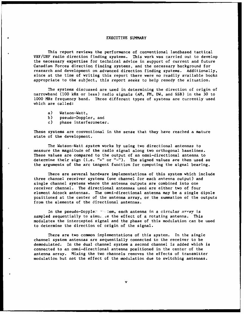
This report reviews the performance of conventional landbased tacticalVHF/UHF radio direction finding systems. This work was carried out to developthe necessary expertise for technical advice in support of current and futureCanadian Forces direction finding systems, and the necessary background forresearch and development on advanced direction finding systems. Additionally,since at the time of writing this report there were no readily available booksappropriate to the subject, this report seeks to help remedy the situation.
The systems discussed are used in determining the direction of origin ofnarrowband (100 kHz or less) radio signals (AM, FM, DW, and SSB) in the 30 to1000 MHz frequency band. Three different types of systems are currently usedwhich are called:
a) Watson-Watt,b) pseudo-Doppler, andc) phase interferometer.
These systems are conventional in the sense that they have reached a maturestate of the development.
The Watson-Watt system works by using two directional antennas tomeasure the magnitude of the radio signal along two orthogonal baselines.These values are compared to the output of an omni-directional antenna todetermine their sign (i.e. "+" or "-"). The signed values are then used asthe arguments of the arc tangent function for computing the signal bearing.
There are several hardware implementations of this system which includethree channel receiver systems (one channel for each antenna output) andsingle channel systems where the antenna outputs are combined into onereceiver channel. The directional antennas used are either two of fourelement Adcock antennas. The omni-directional antenna may be a single dipolepositioned at the center of the antenna array, or the summation of the outputsfrom the elements of the directional antennas.
In the pseudo-Dopple:- . em, each antenna in a circular array issampled sequentially to simu .;.e the effect of a rotating antenna. Thismodulates the intercepted signal and the phase of this modulation can be usedto determine the direction of origin of the signal.
There are two common implementations of this system. In the singlechannel system antennas are sequentially connected to the receiver to bedemodulated. In the dual channel system a second channel is added which isconnected to an omni-directional antenna positioned in the center of theantenna array. Mixing the two channels removes the effects of transmittermodulation but not the effect of the modulation due to switching antennas.
v

In the phase interferometer the phase difference information determinedfrom measurements between spatially separated antennas is used to determinethe direction of origin of the signal.
Implementations of this system include systems with a single receiverfor each antenna, dual channel systems where pairs of antennas are measuredsequentially, and single channel systems which are similar to the dual channelsystems except the outputs from pairs of antennas are combined to preserve thephase information but require only one receiver channel.
There are a number of factors which reduce the accuracy of conventionaldirection finding systems under actual operational conditions. Multipath is amajor problem and can cause errors on the order of several degrees in thebearing estimates [111. Raising the height of the antenna array andincreasing the diameter of the antenna array will (at least theoretically)reduce the effects of multipath. However these solutions tend to conflictwith tactical requirements.
Co-channel interference can cause the bearing to vary rapidly. If thesignal of interest is the strongest, averaging techniques can be used todetermine its bearing. In a Watson-Watt system using a CRT display driven bythe directional antenna outputs, a skilled operator may be able to determinethe direction of the various signals being intercepted.
Equipment is a source of bearing errors, most notably in the antennaswhere mutual coupling between elements or interaction with the localenvironment can corrupt the antenna patterns from their expected response.Calibration techniques can significantly reduce some of these effects to thepoint that manufacturers make claims of equipment accuracies of 1 degree rmsor less.
Noise, both equipment generated and environmental, effects the stabilityof the bearing measurement. Typically these are zero-mean processes so thataveraging can reduce the variations in bearing to suitable levels. Significanterrors can occur if the signal to noise ratio drops below about 10 dB.
In reviewing equipment manufacturers published specifications fordirection finding systems, its was determined that it was not possible tocompare systems in any meaningful sense. The major problem is that there isinsufficient information provided on how the various specifications wereobtained which is critical if effective comparisons are to be made.
vi
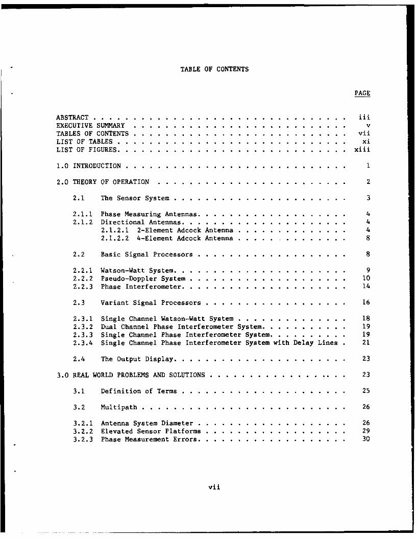
TABLE OF CONTENTS
PAGE
ABSTRACT .................................. iiiEXECUTIVE SUMMARY................................vTABLES OF CONTENTS.................................viiLIST OF TABLES..................................xiLIST OF FIGURES. ............................... xiii
1.0 INTRODUCTION ................................. 1
2.0OTHEORY OF OPERATION ........................... 2
2.1 The Sensor System. .......................... 3
2.1.1 Phase Measuring Antennas .. .................... 42.1.2 Directional Antennas .. .. ... ................. 4
2.1.2.1 2-Element Adcock Antenna .................. 42.1.2.2 4-Element Adcock Antenna ................... 8
2.2 Basic Signal Processors. ..................... 8
2.2.1 Watson-Watt System .. ....................... 92.2.2 Pseudo-Doppler System ......................... 102.2.3 Phase Interferometer. ......................... 14
2.3 Variant Signal Processors .......................16
2.3.1 Single Channel Watson-Watt System. ................. 182.3.2 Dual Channel Phase Interferometer System .. ............ 192.3.3 Single Channel Phase Interferometer System .. ........... 192.3.4 Single Channel Phase Interferometer System with Delay Lines . 21
2.4 The Output Display. ........................ 23
3.0 REAL WORLD PROBLEMS AND SOLUTIONS .......................23
3.1 Definition of Terms .......................... 25
3.2 Multipath ............................... 26
3.2.1 Antenna System Diameter ...................... 263.2.2 Elevated Sensor Platforms .......................293.2.3 Phase Measurement Errors. ..................... 30
vii
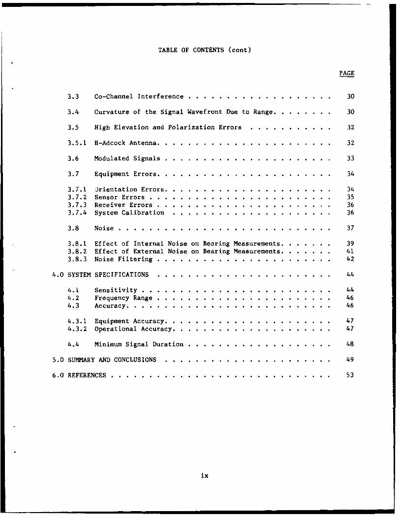
TABLE OF CONTENTS (cont)
PAGE
3.3 Co-Channel Interference ...... ................... .... 30
3.4 Curvature of the Signal Wavefront Due to Range .... ........ 30
3.5 High Elevation and Polarization Errors .. ........... ... 32
3.5.1 H-Adcock Antenna ......... ...................... ... 32
3.6 Modulated Signals ........ ...................... ... 33
3.7 Equipment Errors ........ ....................... .... 34
3.7.1 Jrientation Errors ........ ...................... ... 343.7.2 Sensor Errors ......... ....................... .... 353.7.3 Receiver Errors ........ ....................... .... 363.7.4 System Calibration ........ ..................... ... 36
3.8 Noise ........... ............................ ... 37
3.8.1 Effect of Internal Noise on Bearing Measurements ......... ... 393.8.2 Effect of External Noise on Bearing Measurements ....... .... 413.8.3 Noise Filtering ........ ...................... .... 42
4.0 SYSTEM SPECIFICATIONS ......... ....................... ... 44
4.1 Sensitivity ......... ......................... .... 444.2 Frequency Range ........ ....................... .... 464.3 Accuracy .......... ........................... .... 46
4.3.1 Equipment Accuracy ........ ...................... ... 47
4.3.2 Operational Accuracy ....... ..................... .... 47
4.4 Minimum Signal Duration ....... ................. ... 48
5.0 SUMMARY AND CONCLUSIONS ......... ...................... ... 49
6.0 REFERENCES ........... ............................. .... 53
ix
LIST OF TABLES
PAGE
TABLE 1 SPECIFICATIONS FOR COMMERCIAL CDF SYSTEMS .. .......... .. 51
xi
LIST OF FIGURES
PAGE
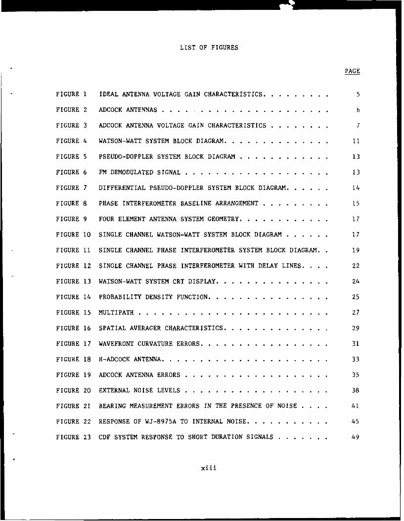
FIGURE I IDEAL ANTENNA VOLTAGE GAIN CHARACTERISTICS ...... ......... 5
FIGURE 2 ADCOCK ANTENNAS . . . ...................... 6
FIGURE 3 ADCOCK ANTENNA VOLTAGE GAIN CHARACTERISTICS ..... ........ 7
FIGURE 4 WATSON-WATT SYSTEM BLOCK DIAGRAM .... .............. .11
FIGURE 5 PSEUDO-DOPPLER SYSTEM BLOCK DIAGRAM ... ............ .. 13
FIGURE 6 FM DEMODULATED SIGNAL ...... ................... ... 13
FIGURE 7 DIFFERENTIAL PSEUDO-DOPPLER SYSTEM BLOCK DIAGRAM ...... .14
FIGURE 8 PHASE INTERFEROMETER BASELINE ARRANGEMENT .......... .. 15
FIGURE 9 FOUR ELEMENT ANTENNA SYSTEM GEOMETRY ... ............ .. 17
FIGURE 10 SINGLE CHANNEL WATSON-WATT SYSTEM BLOCK DIAGRAM ...... 17
FIGURE 11 SINGLE CHANNEL PHASE INTERFEROMETER SYSTEM BLOCK DIAGRAM. 19
FIGURE 12 SINGLE CHANNEL PHASE INTERFEROMETER WITH DELAY LINES. . 22
FIGURE 13 WATSON-WATT SYSTEM CRT DISPLAY ........ ............... 24
FIGURE 14 PROBABILITY DENSITY FUNCTION ..... ................ .25
FIGURE 15 MULTIPATH .......... ......................... .. 27
FIGURE 16 SPATIAL AVERAGER CHARACTERISTICS .... .............. .29
FIGURE 17 WAVEFRONT CURVATURE ERRORS ..... ................. ... 31
FIGURE 18 H-ADCOCK ANTENNA ........ ...................... .. 33
FIGURE 19 ADCOCK ANTENNA ERRORS ...... ................... ... 35
FIGURE 20 EXTERNAL NOISE LEVELS ...... ................... ... 38
FIGURE 21 BEARING MEASUREMENT ERRORS IN THE PRESENCE OF NOISE . ... 41
FIGURE 22 RESPONSE OF WJ-8975A TO INTERNAL NOISE ............. ... 45
FIGURE 23 CDF SYSTEM RESPONSE TO SHORT DURATION SIGNALS ....... .. 49
xiii
1.0 INTRODUCTION
This report reviews the performance of conventional landbased tactical
VHF/UHF radio direction finding systems. This work was carried out to developthe necessary expertise for technical advice in support of current and future
Canadian Forces direction finding systems, and the necessary background forresearch and development on advanced direction finding systems. Additionally,
since at the time of writing this report there were no readily available books
appropriate to the subject, this report seeks to help remedy the situation.
The systems discussed are used in determining the direction of origin of
narrowband (100 kHz or less) radio signals (AM, FM, DW, and SSB) in the 30 to
1000 MHz frequency band. In this report, these systems are referred to simply
as conventional direction finding (CDF) systems.
There are several tactical requirements for CDF systems which include:
a) Accuracy - As accurate as possible. In practice the best
operational accuracy achieved by convcntional DF systems has beenon the order of a few degrees (too inaccurate for targeting
purposes).
b) Automation - Once the system has been tasked to measure a signal
bearing, the bearing should be determined automatically within afew seconds.
c) Mobility - Man-portable or vehicle mounted.
d) Short set up time - 10 to 20 minutes is the longest time a CDF
system would want to remain at any site; anything longer reducesthe survivability of the system. Consequently the set up time is
constrained to be somewhat less than this in order that there is
enough time for signal bearing measurements to be taken.
e) Robustness - Ruggedized to withstand the rigors of a military
environment.
The first requirement, accuracy, is the main focus of this report. The
fundamental limitations in accuracy imposed by nature as a function of thevarious techniques and implementations are discussed in some dctoil.
Technological difficulties are also discussed as well. as various measurement
criteria used to describe system performance.
The second requirement, automation, constrains CDF systems to fixed
antenna arrays. Direction finding techniques that require the antenna to bemoved or rotated to determine the direction of arrival of the signal, are too
slow for modern tactical purposes.
The final three requirements (mobility, short set-up time, and
(robustness) limit CDF systems to being small and light enough to be carried
by man or vehicle, simple to set up, and reliable.
-2-
!9.1_ough many different types of radio direction finding systems exist,
ther" arc only three basic types of CDF systems currently used which meet
these tactical requirements. These systems are:
a) Watson-Watt,b) pseudo-Doppler, and
c) phase interferometer.
These systems are conventional in the sense that they have reached a mature
state of development. For example, the Watson-Watt system was first proposed
in 1926 [11, the pseudo-Doppler system in 1947 [21, and the phase
interferometer system around 1961 [3]. All three systems were originally
developed for direction finding in the HF frequency band, then later modified
for operation at VHF and UHF frequencies.
2.0 THEORY OF OPERATION
The operation of CDF systems can be broken down in terms of three basic
subsystems: the sensor system, the signal processor, and the display. Each
of these subsystems is discussed in the following subsections.
In discussing the theoretical aspects of the operating principles of CDF
systems, several assumptions are implicit (unless otherwise indicated):
1. The signal follows a single, direct, unobstructed path from the
transmitter to the CDF system;
2. There are no interfering signals;
3. The signal wavefront is planar;
4. The angle of arrival of the signal in elevation is 0 degrees;
5. The signal is vertically polarized;
6. The signal is CW;
7. The measurement equipment is perfect;
8. Noise is absent.
The problems with real world systems when these assumptions break down and the
solutions to these problems will be discussed in a later section.
To simplify discussion, a number of terms and conventions have been used
throughout the rest of this report. The term "channel" is used to describe a
signal path through the CDF system. For example, two signals occupying the
same channel, share the same circuitry, but not necessarily the same frequency
band.
The term "receiver front end" is used to describe the first input
stage(s) of the receiver which shift the radio frequency (RF) signal to an
intermediate frequency (IF), amplify it, and pass it through a bandpass
filter. The bandwidth of the filter controls the receiver bandwidth.
Phase delays introduced by equipment components are assumed to be equal
in all signal paths. Under this assumption, phase delays have no effect on
CDF system operation, except where stated otherwise. Amplitude gains and
losses are also assumed to be equal in all signal paths.
-3-
In the text that follows all angular measurements are expressed indegrees where the convention -180 to +180 degrees has also been adopted. Inequations, however, the corresponding radian measure is used.
The arc tangent function used in the form
= arcTan(Y/X)
throughout the discussion uses the signs of X and Y ("+" or "-") to correctly
determine the quadrant of *.
In the mathematical derivations that follow, the RF signal is assumed to
generate a voltage in a matched dipole antenna of the form
S(t) = Vd Sin(wt + y) Volts
where the parameters of the equation are defined in the following paragraph.The phase angle y is defined to be 0 degrees if the dipole is located at thegeometric center of the antenna array of which it is a part.
Finally, a number of parameters are used repeatedly throughout thissection. They are defined here as:
t - time (seconds),
- signal frequency (radians/second),- signal wavelength (meters),- true signal bearing in azimuch referenced to true North (radians),
Oc - bearing computed by the CDF system (radians),d - distance between a pair of antennas (meters),Vd - maximum voltage induced in a matched dipole antenna (Volts),y - signal phase (radians).
2.1 The Sem~or System
The sensor system electrically couples the CDF system to the radiosignal environment. It consists of an array of two or more antennas whichsupply the appropriate signal information to the signal processor. There areessentially two different types of antennas used in the sensor system: phasemeasuring, and directional.
-4-
2.1.1 Phase Measuring Antennas
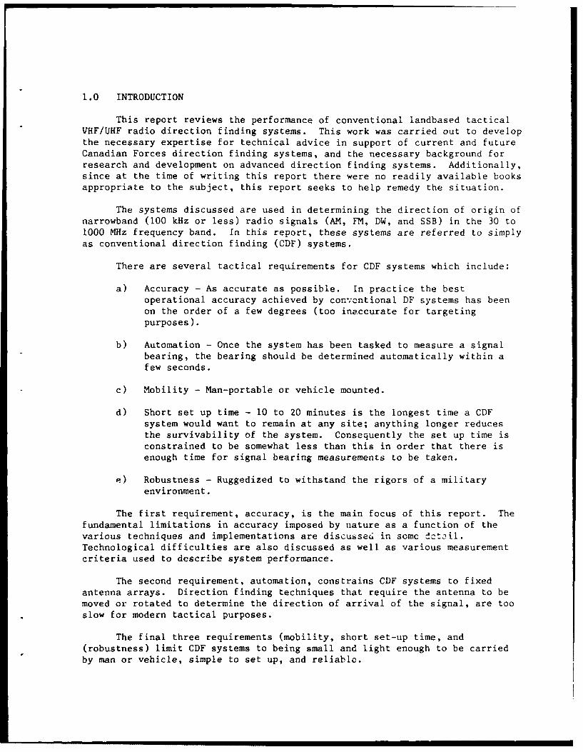
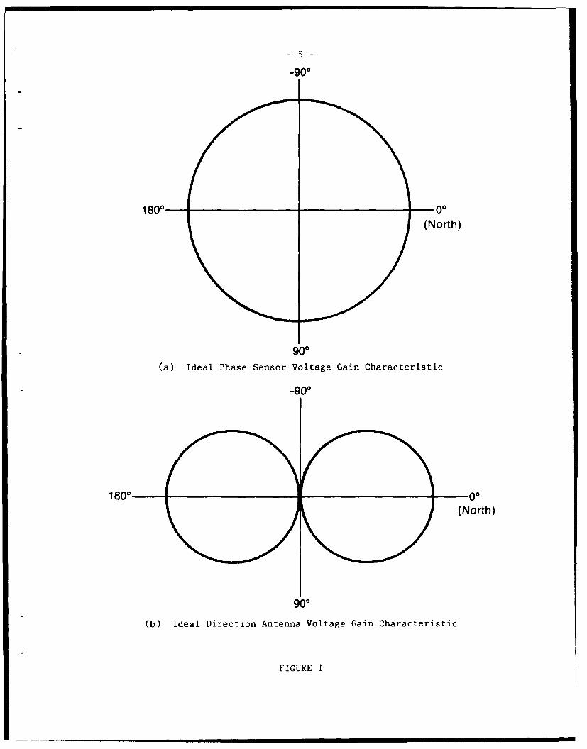
The vertical dipole antenna is used for making phase measurements. Theideal voltage gain pattern (in azimuth) of this antenna (shown in Figure la)is omni-directional, making the antenna equally sensitive to signals arrivingfrom any direction.
Phase measurements are made indirectly. The dipole antenna measures theinstantaneous amplitude of a signal at a specific point in space. The voltagegenerated in the antenna is given by the equation
V(t) = Vd Sin(wt + y) Volts. (1)
By comparing the antenna voltage to a second dipole antenna voltage, therelative phase angles between the two antennas can be determined. In CDFantenna arrays where one antenna is used as a reference (for phase comparisonpurposes), this antenna is known as a "sense" antenna.
2.1.2 Directional Antennas
The ideal voltage gain pattern (in azimuth) of a directional antenna(shown in Figure lb) used for the Watson-Watt system is given by the equation
Gain = Gm Cos(O), (2)
where Gm is the maximum gain of the antenna. Due to the cosine form of thegain equation, this voltage gain pattern is often called the cosine pattern.It is apparent that, unlike the omni-directional phase antenna, the voltagegain of this antenna is highly dependent on the direction of arrival of thesignal.
Real world directional antennas for CDF systems are constructed from twoor more dipole elements. The actual voltage gain patterns are not true cosinepatterns, but rather, approximations of it. Since deviations from the truecosine pattern result in errors in the bearing measurements, design of realworld antenna arrays tries to minimize the cosine deviations.
2.1.2.1 2-Element Adcock Antennas
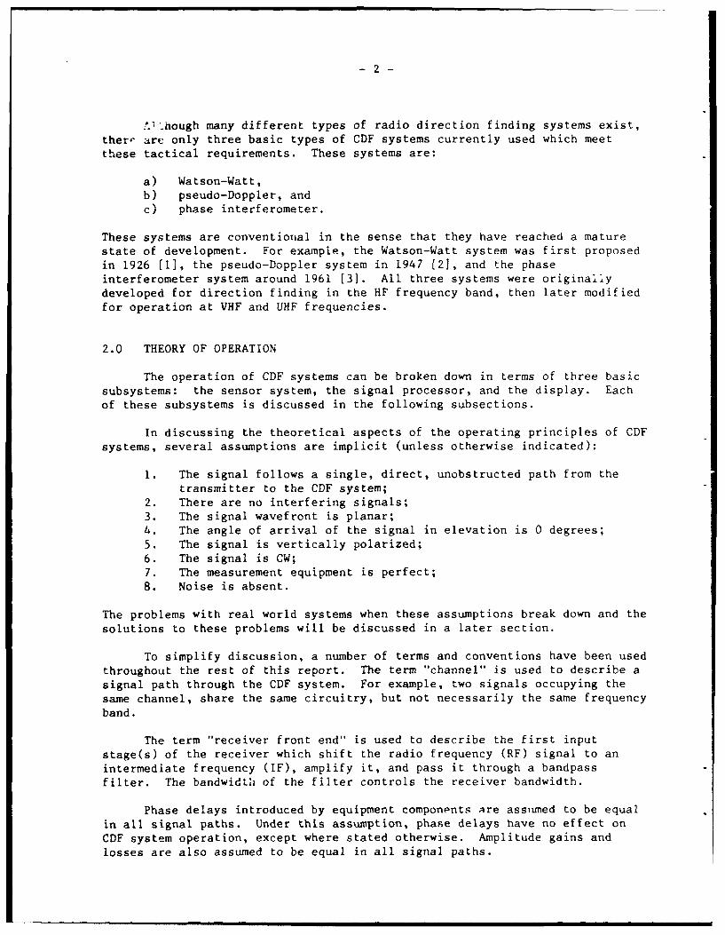
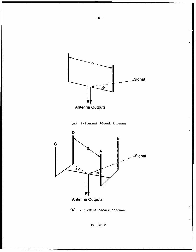
The most commonly used directional antenna is the 2-element Adcockantenna shown in Figure 2a. The output from this antenna is the differencebetween the output voltages of two spatially separated dipole elements. Thevoltage gain is described by the equation
Gain = 2 Gd Sin(n d/X Cos(O)), (3)
where Gd is the gain of a single dipole element.
-900
1800 00
(North)
900
(a) Ideal Phase Sensor Voltage Gain Characteristic
-900
1 8 0 0 --
900
(b) Ideal Direction Antenna Voltage Gain Characteristic
FIGURE 1
6
d
- - -Signal
Antenna Outputs
(a) 2-Element Adcock Antenna
DB
C[I (
-Signal
Antenna Outputs
(b) 4-Element Adcock Antenna.
FIGURE 2
-900d/A=0.75
I " j d/Ak=0.25 I d/,k=0.5
18O~ d/X=0.1
(a) Voltage Gain Characteristics for a 2-Element Adcock Antenna-900
d/X=0.75
/ .-
(b) Voltage Gain Characteristics for a 4-Element Adcock Antenna
FIGURE 3
-8-
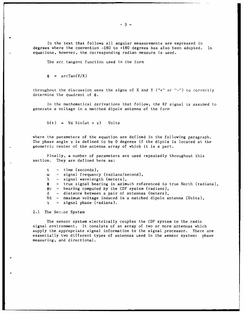
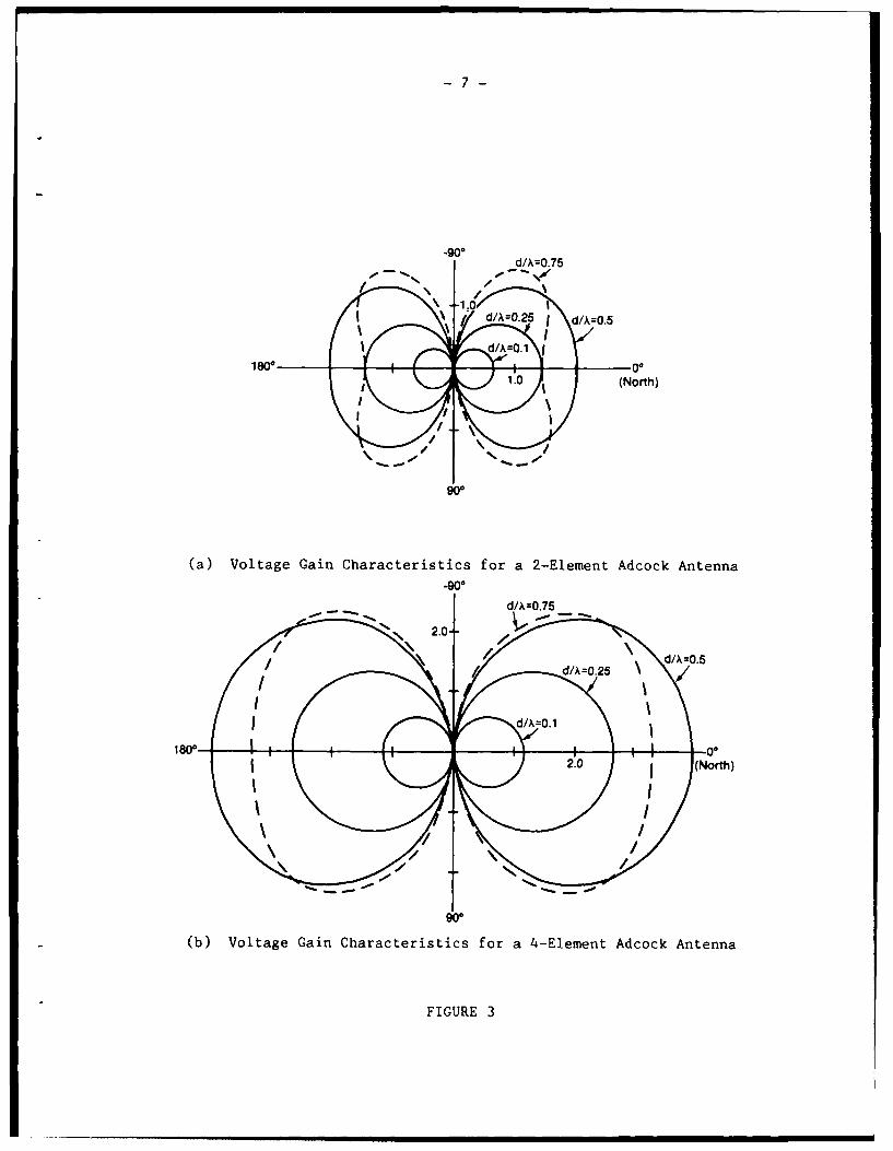
Figure 3a shows the change in gain pattern as the ratio of d/X isvaried. As d/X approaches zero, Equation (3) approaches the ideal cosine formof the equation
Gain = 2Gd (rd/X) Cos(*) (4)
At values of d/X greater than 1/4, the gain pattern begins to departsignificantly from the shape of the ideal cosine pattern. In typical CDFsystems, the maximum ratio of d/X is restricted to 1/4 to minimize the errorsin computed bearing caused by the deviation of the gain pattern from the ideal.
2.1.2.2 4-Element Adcock Antennas
A more complex version of the Adcock antenna is shown in F.gure 2b.This antenna is similar to the 2-element antenna version except each antennaelement has been replaced by a split pair of elements. The output is thedifference in voltage between two summed pairs of elements (A+B and C+D) andthis results in the voltage gain equation given by
Gain = 2 Gd [Sin(Cos(*-a) 7r d/X) + Sin(Cos(*+a) it d/k)] (5)
where "a" is the half angle between summed antenna pairs and is generally avalue between 22.5 and 27.5 degrees.
Figure 3b shows the change in gain pattern as the ratio of d/X isvaried. As d/X approaches zero, Equation (5) approaches the ideal cosine formgiven by
Gain = 4Gd (rd/) Cos(a) Cos(O) (6)
Although not immediately obvious from the gain patterns shown in Figure 3, itwill be shown later that the 4-element Adcock antenna has a much superior gain
pattern than the 2-element antenna, and can be used at ratios of d/Xapproaching 1.0 or more (compared to a ratio of 0.25 for the 2-elementantenna).
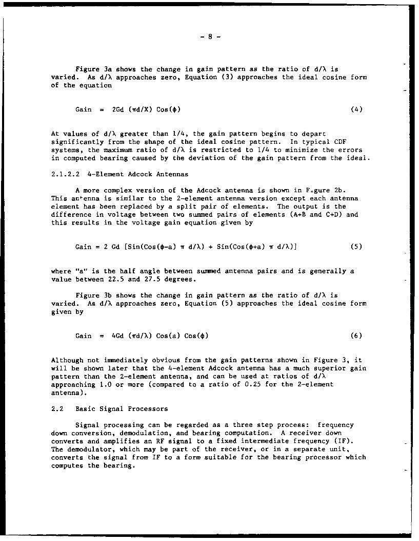
2.2 Basic Signal Processors
Signal processing can be regarded as a three step process: frequencydown conversion, demodulation, and bearing computation. A receiver downconverts and amplifies an RF signal to a fixed intermediate frequency (IF).The demodulator, which may be part of the receiver, or in a separate unit,converts the signal from IF to a form suitable for the bearing processor whichcomputes the bearing.
F-!
-9-
In some systems, the demodulated input signal to the bearing processoris not suitable for audio purposes (i.e. can not be used by the CDF operatorto listen to the intercepted signal). If the demodulator used for the bearingprocessor is separate from the receiver, the receiver demodulator can be usedto convert the signal to audio, otherwise a separate receiver may be requiredfor this purpose.
There are three basic types of CDF systems: Watson-Watt, pseudo-Doppler,and phase interferometer. The signal processing requirements of each of thesesystems are different.
2.2.1 Watson-Watt System
The Watson-Watt system works by measuring the magnitude of the signalvector along two orthogonal axes. These quantities are then used as thearguments of the arctangent function to compute the signal bearing.
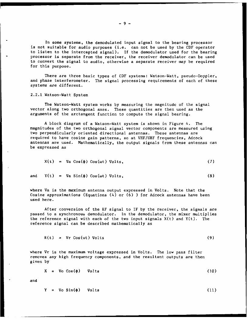
A block diagram of a Watson-Watt system is shown in Figure 4. Themagnitudes of the two orthogonal signal vector components are measured usingtwo perpendicularly oriented directional antennas. These antennas arerequired to have cosine gain patterns, so at VHF/UHF frequencies, Adcockantennas are used. Mathematically, the output signals from these antennas canbe expressed as
X(t) = Va Cos( ) Cos(wt) Volts, (7)
and Y(t) = Va Sin( S ) Cos(wt) Volts, (8)
where Va is the maximum antenna output expressed in Volts. Note that theCosine approximations (Equations (4) or (6) ) for Adcock antennas have beenused here.
After conversion of the RF signal to IF by the receiver, the signals arepassed to a synchronous demodulator. In the demodulator, the mixer multipliesthe reference signal with each of the two input signals X(t) and Y(t). Thereference signal can be described mathematically as
R(t) = Vr Cos(r t) Volts (9)
where Vr is the maximum voltage expressed in Volts. The low pass filterremoves any high frequency components, and the resultant outputs are thengiven by
X = Vo Cos() Volts (10)
and
Y = Vo Sin() Volts (II)
- 10 -
where Vo is the maximum voltage expressed in Volts. The quantities X and Y arethen used to compute the bearing angle using the equation
c = arcTan(Y/X) (12)
The solution to Oc is unique only if the reference is derived from asignal whose phase is independent of the signal bearing. This can be done inone of two ways. In the first method, the output from a dipole sense antenna,positioned at the geometric centre of the array, is utilized. The senseoutput from this antenna can be expressed mathematically as
Se(t) = Vs Sin(wt) Volts (13)
where Vs represents the maximum signal magnitude expressed in volts. In thesecond method, the outputs from each dipole of the Adcock antennas are summedto give the sense output given as
Se(t) = Vs' Sin(wt) Volts (14)
In this case, the magnitude of Vs' has some dependence on the signal bearing,but is always non-zero and positive (no phase dependency) as long as thediameter of the antenna array does not exceed 0.7 of a wavelength. In eithercase, the sense signal is amplified and phase shifted by +90 degrees to givethe required reference signal
R(t) = Vr Cos(wt) Volts (15)
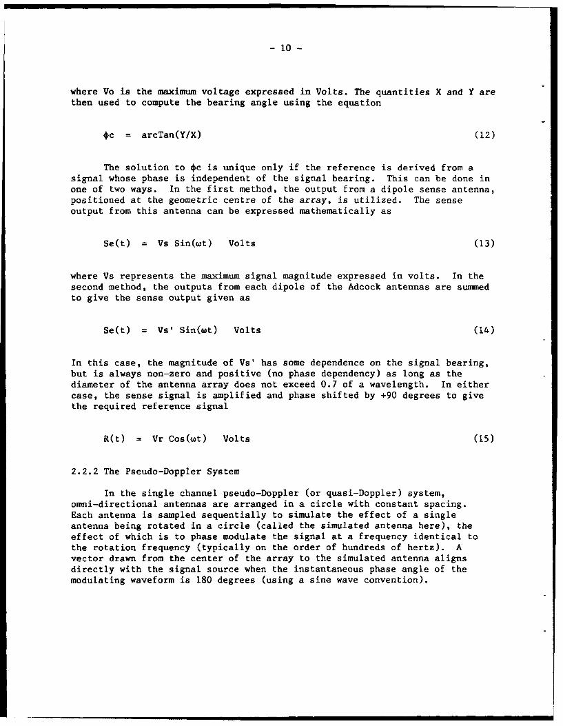
2.2.2 The Pseudo-Doppler System
In the single channel pseudo-Doppler (or quasi-Doppler) system,omni-directional antennas are arranged in a circle with constant spacing.Each antenna is sampled sequentially to simulate the effect of a singleantenna being rotated in a circle (called the simulated antenna here), theeffect of which is to phase modulate the signal at a frequency identical tothe rotation frequency (typically on the order of hundreds of hertz). Avector drawn from the center of the array to the simulated antenna alignsdirectly with the signal source when the instantaneous phase angle of themodulating waveform is 180 degrees (using a sine wave convention).

r -Antenina System n-
W N-- Synchronus-
S () Wats ronat Send Block wDiagram
ofI RFie Filter~
R~t)- rc t)
(b ) eeaton-ofat Ryeferenc S i agamto
(c) Generation of a Reference Signal - Method 2
FIGURE
- 12 -
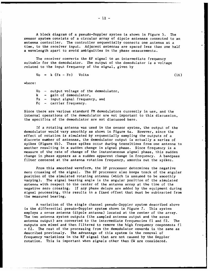
A block diagram of a pseudo-Doppler system is shown in Figure 5. Thesensor system consists of a circular array of dipole antennas connected to anantenna controller. The controller sequentially connects one antenna at atime, to the receiver input. Adjacent antennas are spaced less than one halfa wavelength apart to avoid ambiguities in the phase measurements.
The receiver converts the RF signal to an intermediate frequencysuitable for the demodulator. The output of the demodulator is a voltagerelated to the input frequency of the signal, given by
Vo = k (Fs - Fc) Volts (16)
where:
Vo - output voltage of the demodulator,k - gain of demodulator,Fs - input signal frequency, andFc - carrier frequency.
Since there are various standard FM demodulators currently in use, and theinternal operations of the demodulator are not important to this discussion,the specifics of the demodulator are not discussed here.
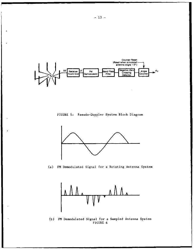
If a-rotating antenna was used in the sensor system, the output of thedemodulator would vary smoothly as shown in Figure 6a. However, since theeffect of rotation is simulated by sequentially sampling the outputs of adiscrete number of antennas, the demodulator output is actually a series ofspikes (Figure 6b). These spikes occur during transitions from one antenna toanother resulting in a sudden change in signal phase. Since frequency is ameasure of the rate of change of the instantaneous signal phase, this suddenchange in phase appears as a sudden apparent change in frequency. A bandpassfilter centered at the antenna rotation frequency, smooths out the spikes.
From this smoothed waveform, the DF processor determines the negativezero crossing of the signal. The DF processor also keeps track of the angularposition of the simulated rotating antenna (which is assumed to be smoothlyvarying). The signal bearing angle is the angular position of the simulatedantenna with respect to the center of the antenna array at the time of thenegative zero crossing. If any phase delays are added by the equipment duringsignal processing, this results in a fixed offset that must be subtracted fromthe measured bearing.
A variation of the single channel pseudo-Doppler system described aboveis the differential pseudo-Doppler system shown in Figure 7. This systememploys a sense antenna (dipole antenna) located at the center of the array.The two antenna system outputs (the sampled antenna output and the senseantenna output) are converted to the intermediate frequencies fl and f2. Theoutputs are mixed and then filtered to remove the high frequency components fl+ f2. The rest of the processing from the demodulator onwards is the same asdescribed previously. The advantage of this system is the removal offrequency variations in the RF signal that are not caused by the Dopplerrotation. This is important when signals other than CW are considered.
-13 -
Counter Reset(Reset when simulatedI I antenna angle = 0) ,
RF IF:,_' " Negative Zero
L \ / , R :I11c041e IV FM I 8.P. Ang~l OI '. l Front Endr-1 Dem dulet°or tlrosig
i oute r - o-g
FIGURE 5: Pseudo-Doppler System Block Diagram
(a) FM Demodulated Signal for a Rotating Antenna System
(b) FM Demodulated Signal for a Sampled Antenna SystemFIGURE 6
- 14 -
2 Punter ntfo eReceiver(Reset when simulaed
Frn Ed Mxe 2antenna angle (r )
FIGURE 7: Differential Pseudo-Doppler System Block Diagram
2.2.3 Phase Interferometer
The phase interferometer, like the pseudo-Doppler system, uses signalphase difference information from spatially separated antennas to determinethe signal bearing. However, unlike the pseudo-Doppler system which processesinformation from each antenna in succession, the phase interferometerprocesses information from two or more antennas simultaneously.
The sensor system of the phase interferometer consists of a non-colineararrangement of at least three dipole antennas. Figure 8 shows the hardwarearrangement for each baseline (where a baseline is defined by two antennas).Since a number of different types of standard phase detectors exist, theiroperation is not discussed here. The output of the phase detector is given bythe equation (refer also to Figure 8)
eij = (2,idij/X) Cos(O - *ij) (17)
If no additional information is known, other than eij, dij, and *ij, then fora single baseline, * has two or ti-re solutions. By constraining the baselineto a length of one half a wavelength or less, exactly two solutions exist (thecorrect solution and the correct solution plus 180 degrees).
- 15 -
The correct solution can be resolved by using multiple baselines, withthe restriction that not all baselines are colinear (i.e. not all values of*ij are the same). The following analysis shows how this can be done.Equation 17 can be rewritten in the form
eij = Aij Sin(O) + Bij Cos( ) (18)
where:
Aij = (21 dij/X) Sin(cij) (19)
and
Bij = (21 dij/X) Cos( ij) (20)
N baselines result in a set of N equations of this form. If the terms Sin($)and Cos( ) are treated as independent variables, say X and Y, these terms canbe determined using standard techniques for solving linear equations (e.g.linear least squares estimate). The computed bearing angle is then given by
c arcTan(Y/X) (21)
SignalIiDpole j
ReceiverFront End
Dipole i ,,Phase N iDetector
Antenna Baseline," Receiver
Front End
FIGURE 8: Phase Interferometer Baseline Arrangement
- 16 -
Under the ideal conditions considered in this section, only twobaselines are required to compute *. However, under realistic conditionswhere a number of error mechanisms are at work (noise for example), a greaternumber of baselines results in a better estimate of the true bearing angle.
A basic requirement of multiple baseline systems is that each uniquesignal direction of arrival results in a unique set of phase measurements toensure unambiguous bearing measurements. This is a function of the geometryof the sensor system and the spacing between sensors, as well as factors whichcause uncertainties in the phase measurements (i.e. noise, measurement errors,etc.). For example, for the geometry shown in Figure 9, neighbouring sensorsmust be somewhat less than one half wavelength apart or bearing ambiguitiesmay result. A more complete discussion on this subject is given in reference[29].
The most common antenna configuration used in phase interferometer CDFsystems is shown in Figure 9. If all six possible baselines are used, itresults in six pairs of equations in the form of Equations (19) and (20).Using the linear least squares method to estimate the values of Sin( ) andCos(*) from these equations, and then computing the estimated bearing anglegives
_1= arcTan /213+ *14 + 023 + 2 241 (22)
L-12- 13 + /2$24 + 0341
2.3 Variant Signal Processors
A number of CDF systems have been designed differently than describedpreviously due to engineering considerations such as cost, availabletechnology, system size, etc. Although the principles behind these systemsare still the same, the hardware implementations are different.
Three such systems will be discussed: the single channel Watson-Wattsystem, the dual channel phase interferometer system, and two different singlechannel phase interferometer systems.
The major difference between the single channel systems and the systemspreviously discussed is the combining of the sensor outputs into one compositesignal so that only a single receiver is required for signal processing.Although this leads to more complicated hardware, the single channel systemshave in the past been easier to implement. This stems from the fact that itis difficult and expensive to build two or more tracking receivers that haveprecisely matched gain and phase characteristics over their full ranges andfrequency ranges. Mismatches in gain and phase between signals can causeserious errors in the bearing calculations. Since in single channel systemsthe input signals share the same receiver channel, the problems encountered inmaintaining the correct gain and phase reiaLlonsitips between signals are farless severe.
-17-
N
Dipole 3 Signal
023
Dipole 4 Dipole 2
Dipole 1
Baseline
FIGURE 9: Four Element Antenna System Geometry
STone 1i I~Generator I-'
An te ) Modulator t : Low Pa ss 'Y
Antenn Filter |
SenseInput Amplifier 90 Receiver arc t OC
N/S x()LwPsAntenna 1 l e n at Filteram
FIGURE 10: Single Channel Watson-Watt System Block Diagram
- 18 -
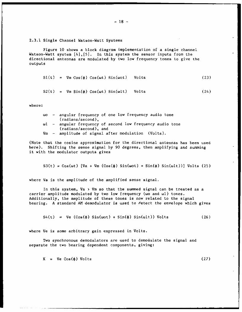
2.3.1 Single Channel Watson-Watt Systems
Figure 10 shows a block diagram implementation of a single channelWatson-Watt system [41,[51. In this system the sensor inputs from thedirectional antennas are modulated by two low frequency tones to give theoutputs
Sl(t) = Vm Cos( ) Cos(wt) Sin(wot) Volts (23)
S2(t) = Vm Sin(O) Cos(wt) Sin(wlt) Volts (24)
where:
wo - angular frequency of one low frequency audio tone(radians/second),
wl - angular frequency of second low frequency audio tone(radians/second), and
Vm - amplitude of signal after modulation (Volts).
(Note that the cosine approximation for the directional antennas has been usedhere). Shifting the sense signal by 90 degrees, then amplifying and sunmingit with the modulator outputs gives
S3(t) = Cos(wt) [Va + Vm (Cos($) Sin(wot) + Sin(O) Sin(wlt))] Volts (25)
where Va is the amplitude of the amplified sense signal.
In this system, Va > Vm so that the summed signal can be treated as acarrier amplitude modulated by two low frequency (wo and wl) tones.Additionally, the amplitude of these tones is now related to the signalbearing. A standard AM demodulator is used to detect the envelope which gives
S4(t) = Ve (Cos(O) Sin(wot) + Sin( ) Sin(wlt)) Volts (26)
where Ve is some arbitrary gain expressed in Volts.
Two synchronous demodulators are used to demodulate the signal andseparate the two bearing dependent components, giving:
X = Ve Cos() Volts (27)
- 19 -
and
Y = Ve Sin() Volts (28)
The reference signals used in the demodulator are derived from the originalmodulating tones with the appropriate phase shifts added to compensate forphase delays in the processed RF signal.
Finally the bearing is calculated from the values X and Y using theexpression
Oc = arcTan(Y/X) (29)
2.3.2 Dual Channel Phase Interferometer System
The dual channel system is very similar to the multi-channel systemdescribed in section 2.2.3 except antenna pairs are sampled in turn, ratherthan simultaneously. This has the advantage of reducing the number ofreceivers required from being equal to the number of antennas used down totwo. The disadvantage is an increase in processing time required to determinethe signal bearing.
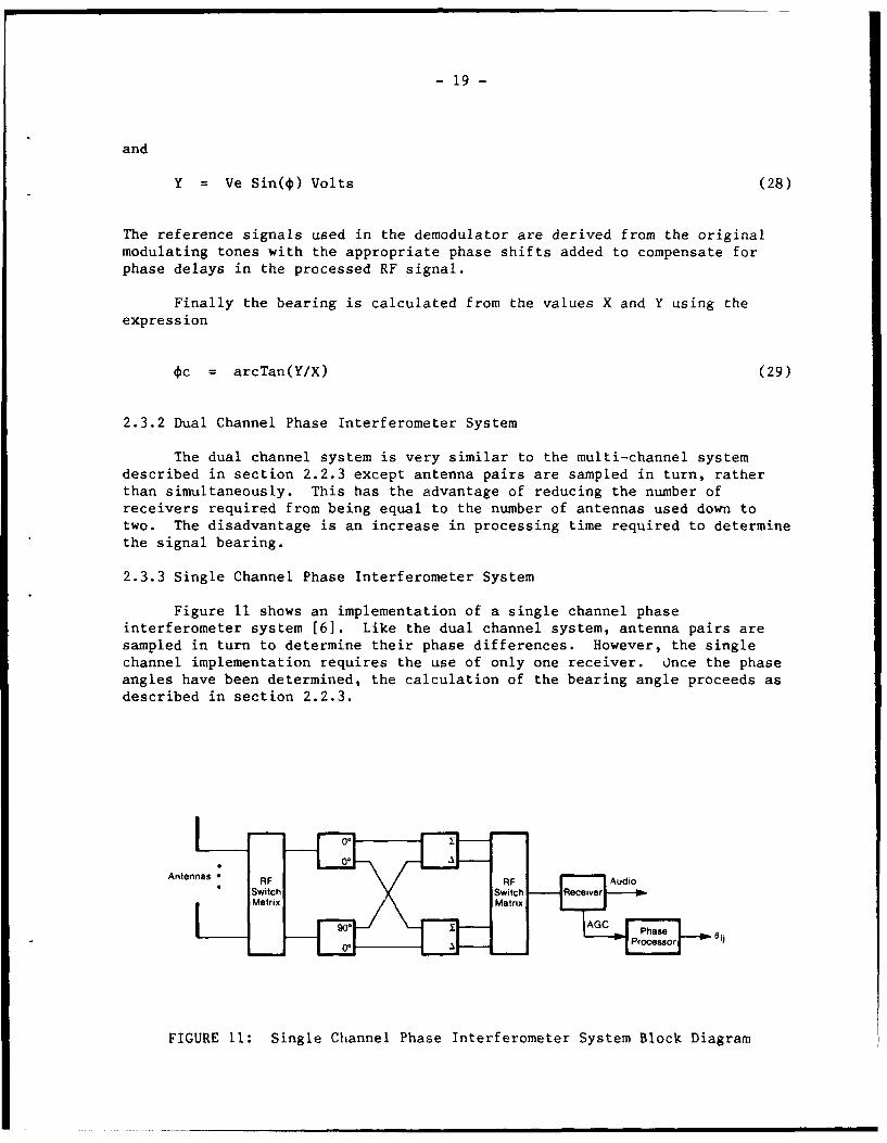
2.3.3 Single Channel Phase Interferometer System
Figure 11 shows an implementation of a single channel phaseinterferometer system [6]. Like the dual channel system, antenna pairs aresampled in turn to determine their phase differences. However, the singlechannel implementation requires the use of only one receiver. Once the phaseangles have been determined, the calculation of the bearing angle proceeds asdescribed in section 2.2.3.
Antennas RF RFAd• Switch Switch R ci e
i Matr xMatrix
0. A Processor
FIGURE 11: Single Channel Phase Interferometer System Block Diagram
- 20 -
To illustrate the operation of this system, assume the outputs from anantenna pair during a measurement period (called the first here) are given by
Si(t) = A Sin(wot + $/2) Volts (30)
and
Sj(t) = B Sin(wot - $/2) Volts (31)
and during the next measurement period are given by
Si(t) = kA Sin(wIt + $/2) Volts (32)
andSj(t) = kB Sin(wlt - $/2) Volts (33)
where:
k - reflects the change in signal level due to amplitude modulation,A - voltage gain of antenna i,B - voltage gain of antenna j,o - angular frequency of signal during first measurement period
(radians/second), and$1 - angular frequency of signal during second measurement period
(radians/second).
During the first measurement period, the outputs from the two antennasare summed and fed to the receiver. If the AGC of the receiver has a linearresponse, the AGC output will be proportional to the amplitude of the sumsignal. This can be expressed as
Vo = c I A2 + B2 + 2AB Cos() Volts (34)
wher- "c" reflects any additional gain to the signal.
During the second measurement period, the difference between the twoantenna output signals is fed to the receiver. The resulting AGC signal willbe
Vi = ck / A2 + B2 - 2AB Cos($) Volts (35)
The two quantities Vo and Vi are then combined in the following manner to give
Vo2 _ Vi2
Xij = (36)
Vo2 + Vi 2
- 21 -
Assuming there is no change in signal amplitude between the first and secondmeasurement periods (i.e., k = 1), then
2AB Cos( )Xij = (37)
A2 + B2
During the third and fourth measurement periods the sum and differencesignals are again used, except this time one antenna output is delayed by90 degrees. Following the previous analysis, the result is given by
2AB Sin(4)Yij = (38)
A2 + B2
From these two quantities, Xij and Yij, the phase angle can be calculated
using the following expression
*ij = arcTan(Yij/Xij) (39)
By applying this measurement sequence to each baseline, the relativephase angles between each antenna pair can be determined. From this point,the calculation of the signal bearing angle is the same as described in
section 2.2.3.
2.3.4 Single Channel Phase Interferometer with Delay Lines
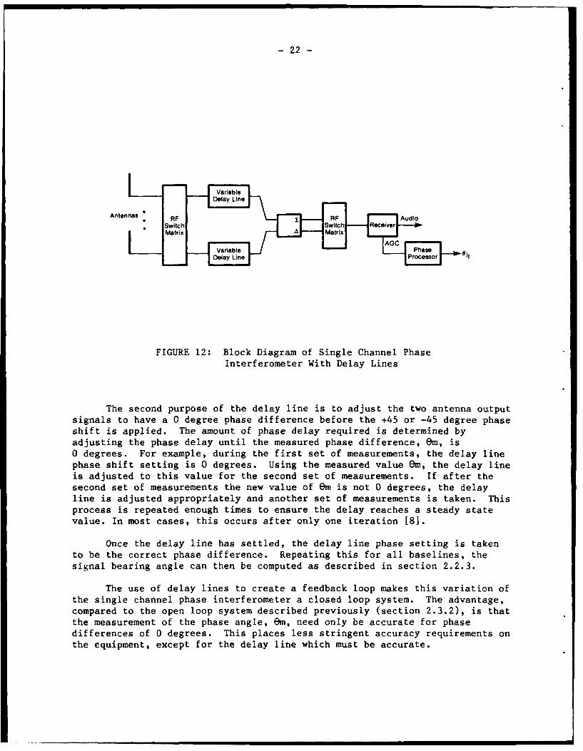
Figure 12 shows an implementation of a single channel phaseinterferometer that uses delay lines [7]. This system is nearly identical inoperation to the single channel phase interferometer just discussed. Themajor difference is the use of delay lines.
The delay lines have two purposes. Instead of delaying one antennaoutput alternately 0 degrees and 90 degrees, the delay lines are used to phaseshift one antenna output alternately +45 degrees and -45 degrees relative tothe other antenna output. The calculation of the measured phase angle betweenpairs of antennas is exactly the same as described in section 2.3.2.
- 22 -
I . . Variable
• 7 Delay Line
Antennas FRAui• Switch Sic - ieSM tr x V a i bl- at i [ G P h a se _ _
ReyiProcessor Oi
FIGURE 12: Block Diagram of Single Channel PhaseInterferometer With Delay Lines
The second purpose of the delay line is to adjust the two antenna outputsignals to have a 0 degree phase difference before the +45 or -45 degree phaseshift is applied. The amount of phase delay required is determined byadjusting the phase delay until the measured phase difference, em, is0 degrees. For example, during the first set of measurements, the delay linephase shift setting is 0 degrees. Using the measured value em, the delay lineis adjusted to this value for the second set of measurements. If after thesecond set of measurements the new value of Em is not 0 degrees, the delayline is adjusted appropriately and another set of measurements is taken. Thisprocess is repeated enough times to ensure the delay reaches a steady statevalue. In most cases, this occurs after only one iteration [8].
Once the delay line has settled, the delay line phase setting is takento be the correct phase difference. Repeating this for all baselines, thesignal bearing angle can then be computed as described in section 2.2.3.
The use of delay lines to create a feedback loop makes this variation ofthe single channel phase interferometer a closed loop system. The advantage,compared to the open loop system described previously (section 2.3.2), is thatthe measurement of the phase angle, Om, need only be accurate for phasedifferences of 0 degrees. This places less stringent accuracy requirements onthe equipment, except for the delay line which must be accurate.
- 23 -
2.4 Output Display
The standard method of displaying the bearing is using a digital displaywith one degree, or one tenth of a degree resolution. Since under actualfield conditions the accuracies of CDF systems are typically on the order ofseveral degrees, one tenth of a degree resolution is virtually meaningless.
Another method of display developed for the Watson-Watt system employs avideo display driven by the outputs of each of the three channels beforedemodulation (i.e. after conversion to IF). The sense channel is used toresolve bearing ambiguity, and the other two channels are used to drive the Xand Y deflection plates of the video display. The appearance of the displayfor various conditions is shown in Figure 13. The main advantages of thisdisplay are that with some operator skill, it is possible to determine thequality of the signal (i.e. noise, co-channel interference, or multipath) aswell as determine the bearings of more than one signal simultaneously.
In some systems, a quality factor is also displayed which is based onparameters derived during the direction finding process. For example, theCommun4 cation Emitter Location System used by the Canadian Army is a singlechannel phase interferometer that uses delay lines. In this particular case,the calculation of the quality factor is based upon signal strength, the fitof the delay line settings to the calibration table data (see section 3.7.4for a discussion on calibration techniques), and the amount of data availablefor computing the mean bearing [71,[8].
In theory, the quality factor should provide an indication of the amountof potential error in the computed bearing angles. In practice, the qualityfactor does not always provide a true indication of the potential error. Theproblem appears to be that the nature of environmental error sources, such asmultipath, are not sufficiently understood to be able to make an accurateassessment of the potential bearing errors.
3.0 REAL WORLD PROBLEMS AND SOLUTIONS
The following discussion deals with the problems and solutionsencountered in the design and operation of real world CDF systems. Thediscussion provides an overview of the problems that occur when theassumptions given previously in Section 2.0 breakdown, the source of theseproblems, and the solutions (if any).
Where more detailed mathematical analysis or the results from computersimulations are provided, they are based on three specific systems. The modelused for the Watson-Watt system is based on the system shown in Figure 4a,with the sense signal derived from the sum of the four dipole outputs(Figure 4c). The pseudo-Doppler system model is based on the single channelversion shown in Figure 5. The phase interferometer system model is based onEquation (22) (see also Figure 8). Frequency and phase demodulators are basedon zero-crossing techniques.

- 24 -
0' (N) 0' (N)
Signal Bearing Signal Bearing
-go- (W)q F D90' (E) -90° (W) 900 (E)
1800(S) 180° (S)
(a) Good Signal (b) Signal Plus Noise
Line of bearing ofinterfering signal 00 (N) 0° (N)
Signal Bearing Signal Bearing
-go- (W)q 90' (E) -90' (W) 90° (E)
180-(S) 180-(S)
(c) Signal Plus One (d) Phase mismatch due tointerfering signal channel misphasing, stray
pickup, or multipath.
FIGURE 13
- 25 -
Mean Value
One Standard Deviationfrom the Mean
PROBABILITY
True Value
MEASUREMENT Rn oVALUE Error
[4 -Bias Error No
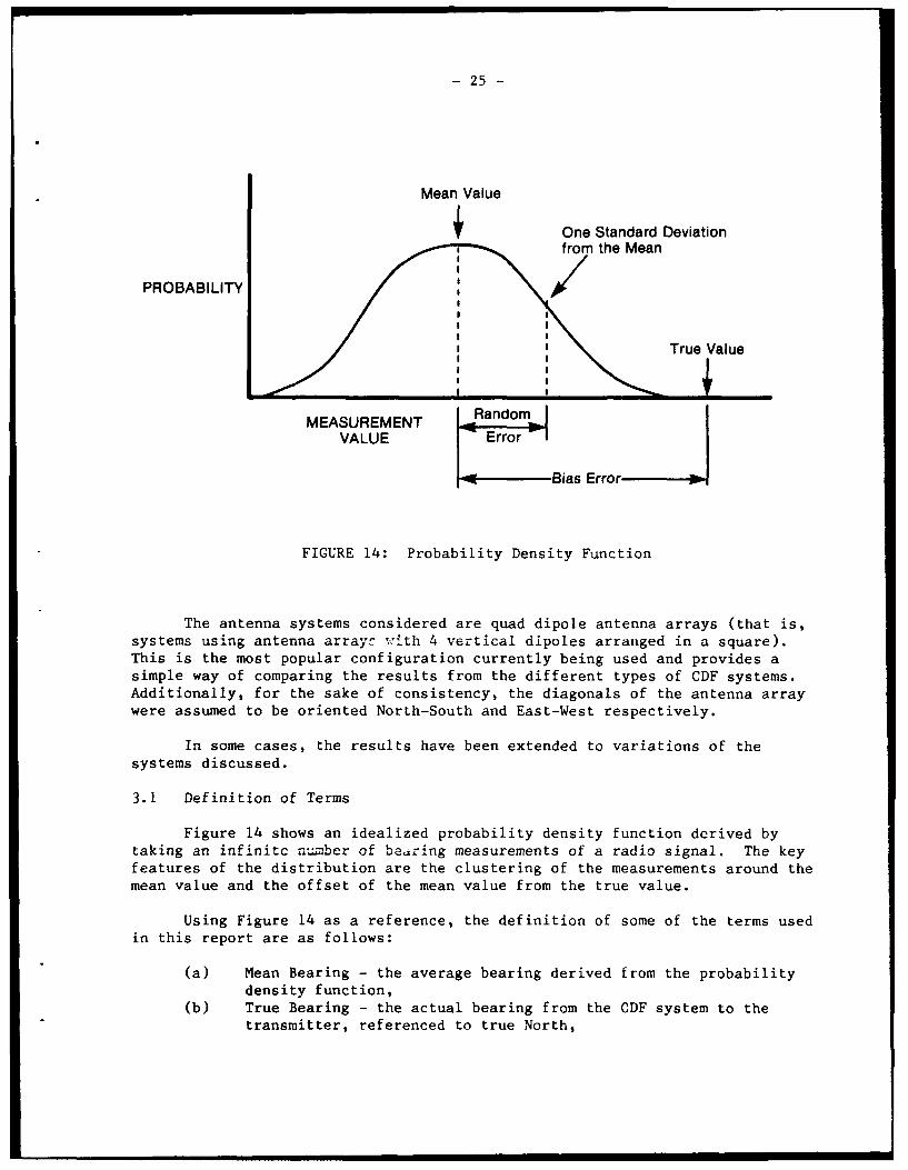
FIGURE 14: Probability Density Function
The antenna systems considered are quad dipole antenna arrays (that is,systems using antenna arrayr with 4 vertical dipoles arranged in a square).This is the most popular configuration currently being used and provides asimple way of comparing the results from the different types of CDF systems.Additionally, for the sake of consistency, the diagonals of the antenna arraywere assumed to be oriented North-South and East-West respectively.
In some cases, the results have been extended to variations of thesystems discussed.
3.1 Definition of Terms
Figure 14 shows an idealized probability density function derived bytaking an infinitc ntber of bedring measurements of a radio signal. The keyfeatures of the distribution are the clustering of the measurements around themean value and the offset of the mean value from the true value.
Using Figure 14 as a reference, the definition of some of the terms usedin this report are as follows:
(a) Mean Bearing - the average bearing derived from the probabilitydensity function,
(b) True Bearing - the actual bearing from the CDF system to thetransmitter, referenced to true North,
- 26 -
(c) Random Error - the standard deviation of random fluctuations inthe bearing measurements due to effects such as noise,
(d) Bias Error - mean bearing minus the true bearing,(e) RMS Error - root mean squared value based on the difference
between the measured value and a reference value (usually thetrue bearing), and
(f) Accuracy - Standard deviation of the bias errors for a number ofmeasurements.
Since most CDF antenna arrays are circular, the diameter "D" has beenused to specify their size.
3.2 Multipath
Multipath occurs when the signal of interest arrives at the receivingantenna via two or more paths. It is also called coherent interference sincethere is a direct signal (the signal of interest) plus indirect interferingsignals, where the interfering signals are delayed copies of the direct signal.
Multipath can occur if any part of the transmitted signal not headeddirectly towards the CDF system is reflected, diffracted, reradiated, orscattered by physical objects (such as rocks, building, or trees) back towardsthe CDF system. The characteristics of multipath (i.e. amplitude, phase,bearing, and number of indirect signals) under tactical operational conditionsare unknown. However, experimental evidence has shown multipath to be thecause of bias errors in CDF systems on the order of several degrees or more[11].
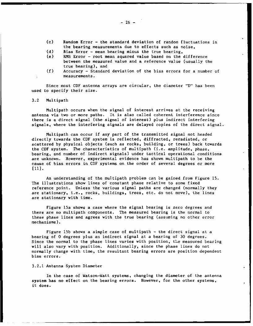
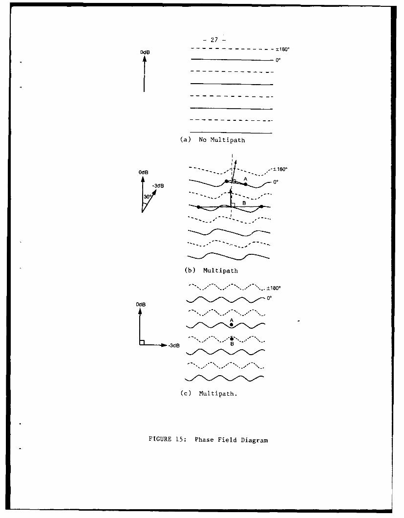
An understanding of the multipath problem can be gained from Figure 15.The illustrations show lines of constant phase relative to some fixedreference point. Unless the various signal paths are changed (normally theyare stationary, i.e., rocks, buildings, trees, etc. do not move), the linesare stationary with time.
Figure 15a shows a case where the signal bearing is zero degrees andthere are no multipath components. The measured bearing is the normal tothese phase lines and agrees with the true bearing (assuming no other errormechanisms).
Figure 15b shows a simple case of multipath - the direct signal at abearing of 0 degrees plus an indirect signal at a bearing of 30 degrees.Since the normal to the phase lines varies with position, t'Le measured bearingwill also vary with position. Additionally, since the phase lines do notnormally change with time, the resultant bearing errors are position dependentbias errors.
3.2.1 Antenna System Diameter
In the case of Watson-Watt systems, changing the diameter of the antennasystem has no effect on the bearing errors. However, for the other systems,it does.
- 27 -
0dB - 180'
t - - - - - -- -- --- 0
(a) No Multipath
S- - - - ' - .'- :1 0
0dB ±--00
-3dB 0
B
(b) Multipath
±1800
OdB
A
-3dB
(c) Multipath.
FIGURE 15: Phase Field Diagram
- 28 -
If the amplitude of the direct signal is greater than the sum of theamplitudes of the indirect signals, averaging the measurements with respect topositicn ran reducc the bias errors. This ;an be accomplished by increasingthe diameter of the sensor system. Comparing the difference in bearing errorsfor baselines A and B in Figure 15b illustrates this effect.
Predicting the exact effect of increasing the antenna diameter is notpossible since a good model of the tactical multipath environment does notexist. However, from theoretical considerations, it is possible to make somegeneralizations. Increasing the antenna diameter will increase the amount ofaveraging, which in turn, will result in more accurate bearings. This is alsosupported by experimental evidence [9]. Additionally, for antenna diametersof less than one half a wavelength of the intercepted signal, spatialaveraging is of little benefit. This is discussed in more detail below.
Examining Figure 15a, the spatial frequency (measured in cycles permeter or cpm) along any baseline will depend on the orientation of thebaseline with respect to the phase lines. The maximum spatial frequency(1I/ cpm) occurs when the baseline is normal to the phase lines and theminimum (0 cpm) when the baseline is parallel to the phase lines. In acomplex wave field composed of coherent signals with various bearings, thespatial frequencies of the signals along any one baseline will vary betweenthese two extremes.
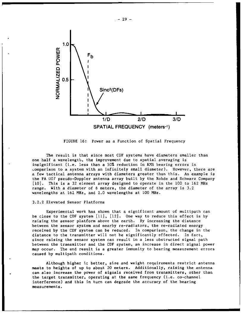
Since averaging is equivalent to a low pass filter operation, the effectof spatial averaging is to suppress the multipath components as a function oftheir spatial frequency. Figure 16 illustrates this suppression. Additionallysince the direct signal is not an error signal, the baseline that determinesthe accuracy of the CDF system is the one closest to being perpendicular tothe transmitter bearing (i.e. parallel with the phase lines). In thisorientation, the spatial frequency of the direct signal will be almost 0 cpmand not affected by averaging.
In figure 16, the spatial bandwidth of the averager, Fb, is a functionof the length of the baseline (or antenna diameter) and is given by thefollowing expression
Fb = 1/2D cpm (40)
Averaging has very little effect if the spatial frequencies of the multipathsignal components are less than Fb. Since the power and spatial frequency ofeach multipath signal components (which depend on their bearing relative tothe baseline) is highly dependent on transmitter and CDF system sitelocations, the advantages of spatial averaging cannot be predicted. However,since the upper frequency limit is defined as l/X, the spatial bandwidth mustbe lower than this value in order for averaging to have any effect. Thistranslates into an antenna diameter of one half a wavelength or more.
- 29 -
1.0a:
3° Fbo:: I0
0 Iw IN ,0.5
a Sinc 2(DFs)o I /
1/D 2/D 3/D
SPATIAL FREQUENCY (meters-)
FIGURE 16: Power as a Function of Spatial Frequency
The result is that since most CDF systems have diameters smaller than
one half a wavelength, the improvement due to spatial averaging isinsignificant (i.e. less than a 50% reduction in RMS bearing errors in
comparison to a system with an infinitely small diameter). However, there are
a few tactical antenna arrays with diameters greater than this. An example isthe PA 007 pseudo-Doppler antenna array built by the Rohde and Schwarz Company
[10]. This is a 32 element array designed to operate in the 100 to 162 MHzrange. With a diameter of 6 meters, the diameter of the array is 3.2wavelengths at 162 MHz, and 2.0 wavelengths at 100 MHz.
3.2.2 Elevated Sensor Platforms
Experimental work has shown that a significant amount of multipath can
be close to the CDF system [11], [121. One way to reduce this effect is byraising the sensor platform above the earth. By increasing the distance
between the sensor system and nearby re-radiators, the re-radiated energyreceived by the CDF system can be reduced. In comparison, the change in the
distance to the transmitter will not be significantly effected. In fact,since raising the sensor system can result in a less obstructed signal path
between the transmitter and the CDF system, an increase in direct signal powermay occur. The end result is a greater immunity to bearing measurement errors
caused by multipath conditions.
Although higher ic better, size and weight requirements restrict antenna
masts to heights of up to about 20 meters. Additionally, raising the antennacan also increase the power of signals received from transmitters, other than
the target transmitter, operating at the same frequency (i.e. co-channelinterference) and this in turn can degrade the accuracy of the bearing
measurements.
- 30 -
3.2.3 Phase Measurement Errors
Figure 15c illustrates a measurement problem that can occur under someconditions. In this situation, dipoles A and B have been designed to bespaced less than one half a wavelength apart so that the absolute phasedifference between the two dipoles will be less than 180 degrees. However,due to the curvature of the phase lines, the absolute phase difference in thisparticular case is greater than 180 degrees. Consequently, the measured phasewill be incorrect (off by 360 degrees). Unless this error is corrected bysome other means, the resultant bearing error may be as much as 180 degrees.
Since this type of phase error occurs more often as the spacing betweenthe dipoles approaches one half of a wavelength, the spacing between adjacentdipoles in CDF arrays are usually restricted to 0.4 wavelengths or less.
3.3 Co-channel Interference
Co-channel interference occurs when one or more interfering signals areat or near the same frequency as the primary signal of interest (i.e. withinthe receiver passband). It is similar to multipath except that theinterfering signals are incoherent; that is, the amplitude, frequency, and/orphase characteristics of the interfering signals have no relationship to the
signal of interest (uncorrelated).
Like multipath, co-channel interference can also be analyzed in terms ofphase lines as illustrated in Figure 15. The main difference between this andthe multipath case is that since the interfering signals are incoherent, thephase pattern is not stationary with respect to time.
In comparison to the multipath case, the improvement in accuracy versusantenna system diameter is the same. Additionally, the problems with phasemeasurement errors that occur for dipole spacings near one half of awavelength are also the same. The major difference is that since the phaselines are not stationary, the bearing errors vary with time; that is, they arerandom errors.
As long as more than half the received signal power is in the signal ofinterest (otherwise the system may lock onto the wrong signal), and phaseerrors do not occur, the bearing fluctuations can be treated as noise andfiltered out. The statistics of this noise will depend on the frequency,modulation, and power of the signals involved. A detailed analysis is beyondthis report, however, a discussion of various types of noise and the effectsof noise filtering are given in Section 3.8.
3.4 Curvature of the Signal Wavefront Due to Range
In the discussion on theory of operation of CDF systems it was assumedthat the signal wavefront could be modelled as a planar waveform. Thisapproximation becomes erroneous if the CDF system - the sensor system inparticular - is located too close to the signal source compared to thediameter of the antenna array.
- 31 -
Distance to source = 5d
0.15
0.10
® 0.05
a: 360o 0.00 '
M: 100 200 30wcn -0.05 -
-0.10
-0 .1 5 -,BEARING ANGLE (degrees)
(a) Bias Error as a Function of Antenna Orientation
10-
0.1
ClI-
D
-J0C'0.01-
- 0.001x 5 10 15 20
DISTANCE TO SOURCE (-d)
(b) Bias Error as a Function of Distance
FIGURE 17: Wavefront Curvature Errors Due to ShortDistances Between Receiver and Transmitter
- 32 -
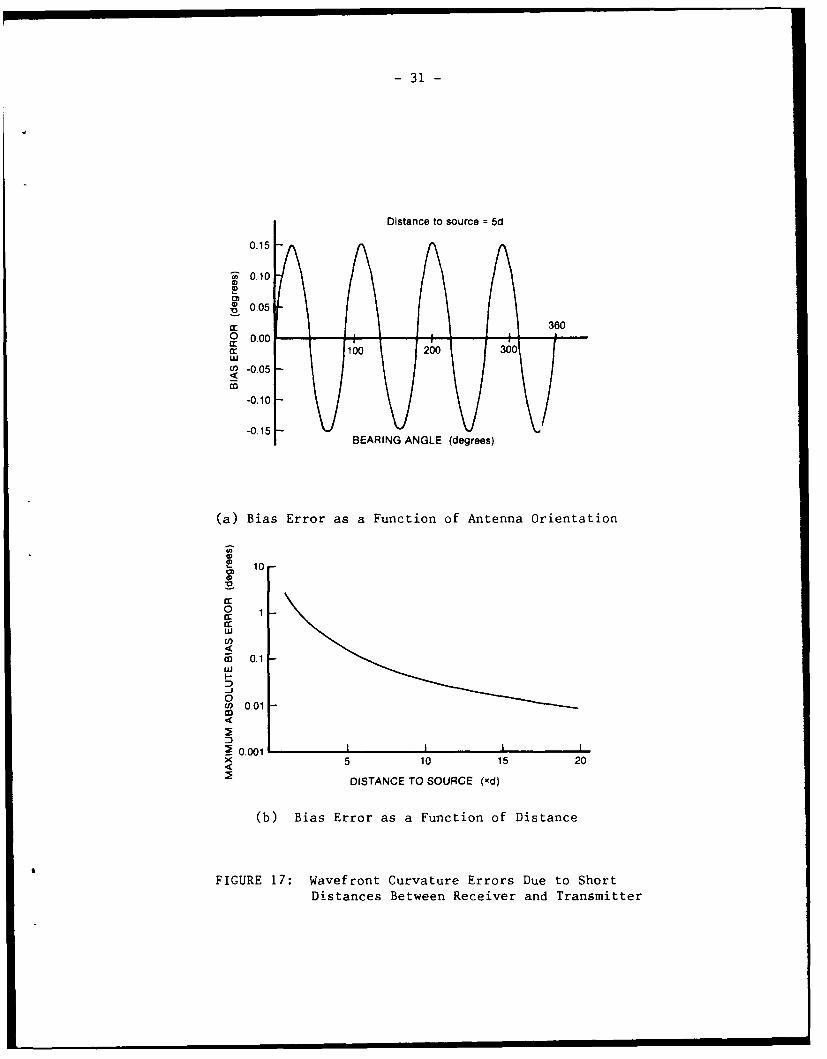
The effect on the bearing measurements is to cause bias errors that aredependent on both the direction of the signal and the distance to the signalsource. Using the computer models, the magnitude of these errors areillustrated in Figure 17. These results are independent '%f signal frequency.
Due to the symmetry of the antenna geometry with respect to the signalwavefront, measurement bias errors cancel out at bearing intervals of 45degrees, starting at 0 degrees. For systems using greater numbers of dipoleelements in a circular configuration (e.g. 8 element pseudo-Doppler arrays),the number of 0 degree error points is greater and the maximum error smaller.
For tactical systems, wavefront curvature errors due to range are not aconsideration. Under wartime conditions, if an enemy transmitter was closeenough to cause errors greater than 0.1 degrees, he is close enough to see!
3.5 High Elevation and Polarization Errors
Ideally CDF sensor systems are insensitive to horizontally polarizedsignals and high elevation angle signals. This is a desirable feature sincegenerally, for landbased tactical systems, the direct signal is verticallypolarized and arrives at a low elevaticn ar6 le. High elevation components andhorizontally polarized components occur only as a result of reflection,diffraction, reradiation, etc. of the signal. Since indirect signalcomponents cause errors, suppression of these components is desirable.
Vertical dipole antennas have a sensitivity that decreases approximatelyas the cosine of the signal elevation angle. Under normal conditions highelevation angle signals are not a factor in the VHF/UHF range. However, undersome unusual conditions (e.g. in northern or southern regions during auroralactivity, signals in the 100-450 MHz may be reflected off the ionosphere) itis possible for high elevation angle signals to cause errors identical tothose discussed under multipath.
Theoretically, vertical dipole antennas are insensitive to horizontallypolarized signals. However, feed lines joining the antennas are susceptibleto picking up unwanted horizontally polarized signal energy. This in turn canaffect the phase and amplitude of the antenna output signal and ultimately thebearing measurement.
Methods of reducing stray pick up include proper grounding of theequipment, minimizing the distance between the antenna system and receiver(s)or placing the first signal amplifying stage right in the antenna head,correctly matching impedances in the antenna system over the frequency band ofoperation, and elevating the sensor system (discussed previously).
3.5.1 H-Adcock
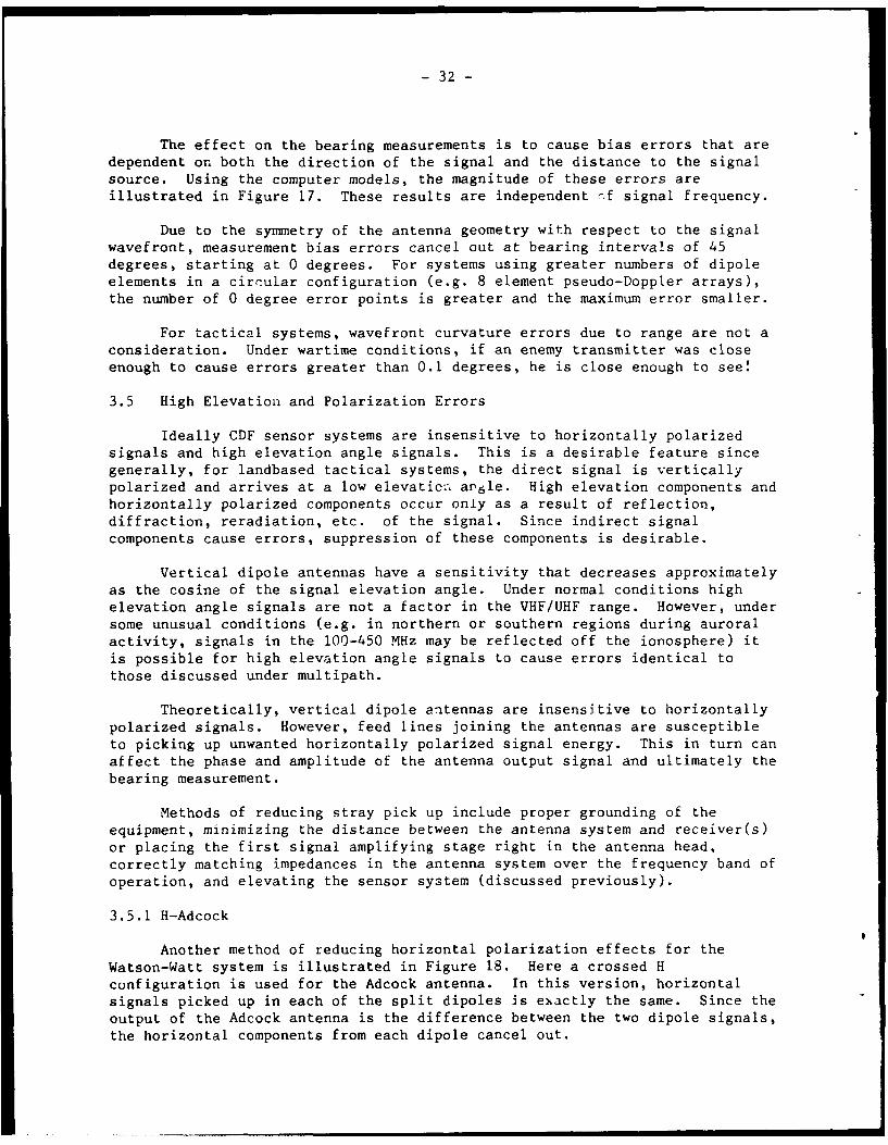
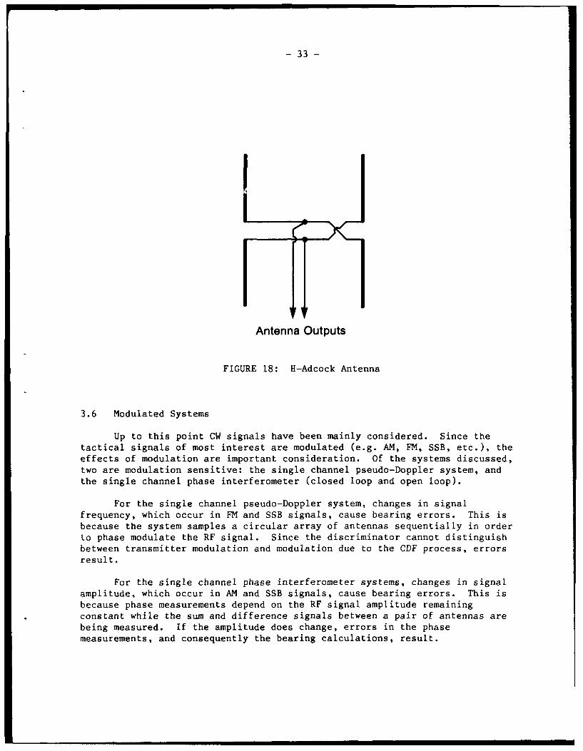
Another method of reducing horizontal polarization effects for theWatson-Watt system is illustrated in Figure 18. Here a crossed Hconfiguration is used for the Adcock antenna. In this version, horizontalsignals picked up in each of the split dipoles is exactly the same. Since theoutput of the Adcock antenna is the difference between the two dipole signals,the horizontal components from each dipole cancel out.
- 33 -
Antenna Outputs
FIGURE 18: H-Adcock Antenna
3.6 Modulated Systems
Up to this point CW signals have been mainly considered. Since thetactical signals of most interest are modulated (e.g. AM, FM, SSB, etc.), theeffects of modulation are important consideration. Of the systems discussed,two are modulation sensitive: the single channel pseudo-Doppler system, andthe single channel phase interferometer (closed loop and open loop).
For the single channel pseudo-Doppler system, changes in signalfrequency, which occur in FM and SSB signals, cause bearing errors. This isbecause the system samples a circular array of antennas sequentially in orderto phase modulate the RF signal. Since the discriminator cannot distinguishbetween transmitter modulation and modulation due to the CDF process, errorsresult.
For the single channel phase interferometer systems, changes in signalamplitude, which occur in AM and SSB signals, cause bearing errors. This isbecause phase measurements depend on the RF signal amplitude remainingconstant while the sum and difference signals between a pair of antennas arebeing measured. If the amplitude does change, errors in the phasemeasurements, and consequently the bearing calculations, result.

- 34 -
Bearing errors resulting from modulation of the RF carrier can beanalyzed in a manner similar to errors resulting from noise. The statisticsof this modulation "noise" are dependent on the modulation type, the amount ofmodulation, and the information content. A more detailed discussion on noiseis given in Section 3.8. Noise filtering techniques which Lre used tosuppress these modulation effects are also discussed. An example of theusefulness of this method is the Watkins-Johnson WJ-8975A, a single channelpseudo-Doppler system. In tests at DREO, the noise filter was able tocompletely suppress the modulation effects of a voice modulated FM signal (theintegration time constant was 2 seconds).
In the other CDF systems discussed, signal modulation can actually bebeneficial for two reasons. The first reason is that signal modulationresults in an averaging of the bearing measurements over a band offrequencies. Since multipath conditions and imperfections in the CDFequipment cause bias errors that vary with frequency, this frequencyaveraging, in general, results in a better estimate of the true bearing.Unfortunately, for narrowband signals (100 kHz or less) the improvement isgenerally insignificant.
The second reason (discussed previously in Section 2.4) is that if avideo display is used to display the orthogonal bearing components of thesignal, it is often possible to determine the direction of non-coherentinterfering signals (as well as the signal of interest) from the display.
3.7 Equipment Errors
A number of sources of bearing error are a result of the equipmentitself. A description of errors due to the orientation of the sensor system,non-ideal responses of the sensor system and receiver, as well as a method ofreducing the impact of these errors, follows.
3.7.1 Orientation Errors
One aspect of CDF systems not previously discussed is the method used todetermine the orientation of the sensor system with respect to true north.The most common method is to align the system using the Earth's magnetic fieldand then apply an offset equal to the local magnetic deviation to the bearingmeasurements.
Systems that use the Earth's magnetic field to determine antennaorientation employ either a compass or a flux gate magnetometer. The compassis used to manually align the antenna using magnetic north as a reference.Systems using the fluxgate magnetometer are more sophisticated. Theycontinuously monitor the antenna system orientation and apply the appropriatecorrection to the bearing measurements automatically.
Another method of orienting the sensor system is by sighting on a knowndistant object. Using a map, the bearing of the distant object can bedetermined, and the sensor system then correctly aligned.
- 35 -
Errors in orienting the sensor system are critical since they translatedirectly into bias errors in the bearing measurements. Random errors can alsoresult, in the case of the fluxgate magnetometer, when high winds shake thesensor system.
3.7.2 Sensor Errors
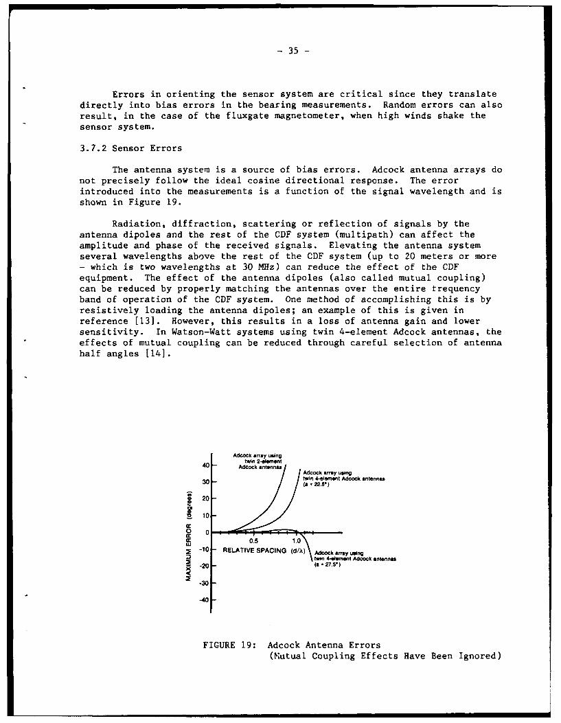
The antenna system is a source of bias errors. Adcock antenna arrays donot precisely follow the ideal cosine directional response. The errorintroduced into the measurements is a function of the signal wavelength and isshown in Figure 19.
Radiation, diffraction, scattering or reflection of signals by theantenna dipoles and the rest of the CDF system (multipath) can affect theamplitude and phase of the received signals. Elevating the antenna systemseveral wavelengths above the rest of the CDF system (up to 20 meters or more- which is two wavelengths at 30 MHz) can reduce the effect of the CDFequipment. The effect of the antenna dipoles (also called mutual coupling)can be reduced by properly matching the antennas over the entire trequencyband of operation of the CDF system. One method of accomplishing this is byresistively loading the antenna dipoles; an example of this is given inreference [131. However, this results in a loss of antenna gain and lowersensitivity. In Watson-Watt systems using twin 4-element Adcock antennas, theeffects of mutual coupling can be reduced through careful selection of antennahalf angles [14].
Adcock array usingtwin 2-element
40 - Adcock antennas~k anenn/ Adcock array usingtwin 4-element Adcock antennas(s = 5")
20 -
10 10
0oiw 0.5 1.0IM -10 - RELATIVE SPACING (d/ Adcock array usingD tin 4-eemrent Adcock antennas
.2 _ (a = 27.5')
-30
-40
FIGURE 19: Adcock Antenna Errors
(Mutual Coupling Effects Have Been Ignored)
- 36 -
At UHF frequencies the wavelengths are small enough that shadowing ofthe antenna elements by the antenna mast can occur. This can cause gainimbalances between shadowed and unshadowed elements of the order of 20 dB ormore, which in turn can cause errors of several degrees or more in the bearingmeasurement [15].
Other problems include impedance mismatches between the antenna and therest of the CDF system, misalignment of the antenna elements, and poormatching of phase and gain characteristics between separate antennas. Carefulattention to the design and construction of the antenna system is required tokeep the effects of these problems on the bearing measurements to a minimum.
3.7.3 Receiver Errors
Ideally, the gain characteristics of the receiver channels are linearand the delays are constant over the signal bandwidth, so that the receiveroutput signal is a good representation of the signal of interest.Additionally, in multichannel systems, the gain and phase characteristics ofeach channel would be matched to preserve the correct relationship betweensignals in different channels.
In real world systems it is impossible to meet these requirements, andthe result is bias errors in the bearing measurements. For example, a 4%error in the measurement of the amplitude of one Adcock antenna output couldresult in a bearing error of up to 1 degree in a Watson-Watt system.Similarly, in the measurement of phase differences of a four element phaseinterferometer, a 4% error along a single baseline (which equates to I and 5degree phase errors for antenna system diameters of 0.5 and 0.1 wavelengthsrespectively) could result in bearing errors up to I degree.
If the variations from ideal responses are small enough, thecorresponding errors in the bearing measurements will be tolerable.
3.7.4 System Calibration
Since the measurement errors that have been described are bias errors,they can 'y corrected to some extent by calibrating the system. There are twomethods commonly used to calibrate CDF systems.
The first method compensates for time variant system errors. Acalibration circuit simulates a signal arriving from a known direction(usually 0 degrees). The operator adjusts a bearing offset control until thediplayed bearing is correct.
The second method compensates for time invariant frequency and bearingdependent errors. This procedure works by comparing the calculated bearing,or the output of an intermediate stage, to the values in a calibration tablethat has been organized on the basis of bearing versus frequency. Bycomparing the measured data with the calibrated data at the appropriatefrequency, the correct bearing can be determined. This is done by finding theclosest match between the measured data and the calibrated data. Byinterpolating from the calibrated data using the closest match and itsneighbours, a good estimate of the bearing position can be made. Once theapparent bearing position of the measured data has been determined, thecorrected bearing angle can be found.
- 37 -
To generate the look-up table, the CDF equipment is placed on a largeturntable at a calibrated site (i.e. site errors are accounted for). Atransmitting antenna transmits a signal at one frequency while the turntableis slowly turned 360 degrees. Bearing measurements are taken at fixed angleincrements and the appropriate measurements are stored in the table. Thefrequency is incremented and the process is repeated until the entirefrequency range has been covered. For example, ESL makes calibrationmeasurements every 3 degrees for each of 30 frequencies to cover the20-150 MHz band of the Canadian Army's Communications Emitter Location System(a single channel phase interferometer system which uses delay lines) [8].
Since there is often some uncertainty in the measured bias errors due torandom effects such as noise, the calibration data is smoothed to removeextraneous values, and then stored in memory in a tabular form.
The smaller the direction and frequency increments in the calibrationprocess, the more accurate the method, since interpolation errors will bereduced. However, the increase in accuracy comes at the price of morecalibration data, larger memory, and increased processing time.
The methods of calibration described here compensate for a largepercentage of the measurement bias errors introduced by the equipment. Infact, calibration can reduce equipment errors from several degrees to lessthan a degree. However, bias errors introduced into the measurements bychanges that occur over time and which are dependent on frequency, bearing,phase, or amplitude, etc., can not be compensated for by the calibrationmethods discussed.
3.8 Noise
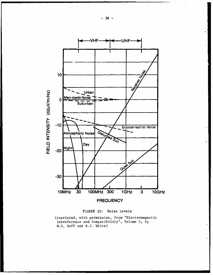
The effect of noise on the performance of CDF systems is to degrade theaccuracy and precision of the bearing measurements. The major sources ofnoise in the VHF/UHF band are shown in Figure 20 [16]. The levels shown inFigure 20 are the noise levels that would be measured at the output terminalsof a dipole antenna matched at all frequencies.
Of primary interest to CDF systems are three types of noise: internalnoise, extraterrestrial noise, and man-made noise. A description of thesetypes of noise follows.
Internal noise is generated primarily in the input sectioh of the CDFsystem which includes the first amplifying stage of the receiver. There arethree distinct sources of internal noise (for solid state devices), namely,flicker noise, shot noise, and thermal noise [17].
Extraterrestrial noise is produced by a large number of radio sourcesdistributed principally along the galactic plane (galactic noise) plus noisefrom the sun. The noise contribution from the sun is variable and periodicwith an eleven year cycle. It generates the highest noise levels duringperiods of peak sunspot and solar flare activity.
- 38 -
10F 106oH
100
-.UrbanMan-made Noise ___-- _._.
E i0
Suburban
cn -10 Extraterrestrial NoisezU.1 Atmospheric Noisez
u. NgDay lit
-30
10MHz 30 100MHz 300 1GHz 3 10GHz
FREQUENCY
FIGURE 20: Noise Levels
(reprinted, with permission, from "ElectromagneticInterference and Compatibility", Volume 5, byW.G. Duff and R.J. White)
- 39 -
Man-made noise is produced by intentional radiators such as radiostations, radars, radio beacons, etc., as well as unintentional radiators suchas power lines, electric tools, fluorescent lights, etc.
The major differences between the three types of noise described are inthe statistical nature of the noise. Depending on the type of noise thatdominates, this, in turn, affects the statistical nature of the resultingbearing errors.
Internal noise can be accurately modelled in the VHF/UHF band as whiteGaussian noise. Ignoring noise components outside the CDF system passband,the internal RMS noise can be described using the equation
Pn = 30 + lOLog(kTB) + F dBm (41)
where:
k - Boltzman's constant (1.38 x 10⁻²³ joules per K),T - temperature (293K at room temperature),B - bandwidth (Hz), andF - noise figure of receiver (typically about 10 dB).
Extraterrestrial and man-made noise can be modelled in the VHF/UHF bandas white Gaussian noise plus impulse noise [181,[19]. Of the two types,man-made noise is generally more impulsive in nature. However, the strengthof the impulse component is highly dependent on the exact nature of the noisesources. The approximate RMS noise levels of man-made and extraterrestrialare shown in Figure 20.
The type of noise that dominates, is dependent on frequency, location,and antenna gain. The effects of frequency and location are apparent inFigure 20. Additionally, although not shown, man-made noise levels in remoterural areas are typically lower than extraterrestrial noise levels. Antennagain affects the ratio between internal noise and external (man-made plusextraterrestrial) noise. In operational CDF systems, design constraintsresult in antenna systems that do not have optimum gain characteristics overthe complete operational frequency spectrum as was assumed in Figure 20.Consequently, in some systems (especially in quiet rural environments)internal noise may be stronger than the external noise.
It should be recognized that Figure 20 does not indicate man-made noiselevels for the tactical wartime environment. Wartime levels would doubtlesslybe greater, but the actual levels are impossible to predict.
3.8.1 Effect of Internal Noise on Bearing Measurements
To examine the effects of internal noise alone, the theoreticalperformance of each of the three CDF systems in the presence of internal noisewas simulated on a computer. Noise was considered to be the only errorproducing mechanism.
- 40 -
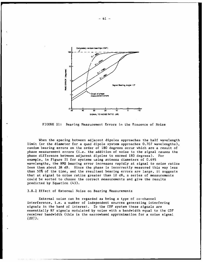
Figure 21 shows the results. The signal to noise ratio refers to thelevels measured at the output of each dipole element (which were equal for allfour dipoles). These values can be converted to the corresponding maximumsignal to noise ratios at the output of an Adcock antenna using the expression
SNR(Adcock) = SNR(Dipole) + 20Log(Gain/N) dB (42)
where for a twin 2-element Adcock antenna system the parameter "Gain" is givenby equation (3) and N = 2, and for a twin 4-element Adcock antenna system theparameter "Gain" is given by equation (5) and N = 4. The errors shown are fora single measurement without noise filtering (as discussed in Section 3.8.3).
In Figure 21 the noise was additive white Gaussian noise generatedinternally (i.e. the noise voltages measured at each dipole wereuncorrelated). In this case the response of the three different systems wasalmost identical.
For signal to noise ratios greater than 10 dB, and antenna arraydiameters one half wavelength or less, the RMS bearing errors due to noise canbe approximated by the formula
-SNR/20Error = 10 * 90x/(lr2D) degrees (43)
where SNR is the signal to noise ratio in dB.
At signal levels less than 10 dB, multiplication of the noise withitself (called multiplicative noise) in nonlinear operations (such as receiverdetector circuits or the arc tangent operation) begins to dominate. Theresult is a decrease in the signal to noise ratio and a change in thefrequency distribution and bandwidth of the noise. Modelling these effects isbeyond the scope of this report since it is specific to the exact manner inwhich the bearing is actually generated. The result, however, is pooreraccuracy than would be expected otherwise.
At very low signal levels, the bearing error levels off as it approachesthe upper limit (104 degrees is the RMS error when the bearings are completelyrandom, that is, equally distributed in all directions).
"~ i l l l l i mmmn an Uilmlel l-
- 41 -
t mpletly random bearings (104)
0 1Ww Signal Bearing Angle =
' Onsst of phas1measurement erron
50 40 30 2 10 0 -10
SIGNAL TO NOISE PATIO (dB)
FIGURE 21: Bearing Measurement Errors in the Presence of Noise
When the spacing between adjacent dipoles approaches the half wavelength
limit (or the diameter for a quad dipole system approaches 0.707 wavelengths),random bearing errors on the order of 180 degrees occur which are a result ofphase measurement errors (i.e. the addition of noise to the signal causes thephase difference between adjacent dipoles to exceed 180 degrees). For
example, in Figure 21 for systems using antenna diameters of 0.695wavelengths, the RMS bearing error increases rapidly at signal to noise ratiosless than about 38 dB. Since the phase is incorrectly measured this way lessthan 50% of the time, and the resultant bearing errors are large, it suggeststhat at signal to noise ratios greater than 10 dB, a series of measurements
could be sorted to choose the correct measurements and give the resultspredicted by Equation (43).
3.8.2 Effect of External Noise on Bearing Measurements
External noise can be regarded as being a type of co-channel
interference, i.e. a number of independent sources generating interferingsignals in the band of interest. To the CDF system these signals areessentially RF signals modulated by noise with a bandwidth equal to the CDFreceiver bandwidth (this is the narrowband approximation for a noise signal[201).
- 42 -
The main difference between internal noise and external noise, otherthan signal statistics (i.e. Gaussian versus impulsive), is the correlationbetween antenna dipole voltages. Internal noise is assumed to be uncorrelatedregardless of antenna spacings. External noise is totally correlated forantenna spacings of 0 wavelengths, and gradually becomes uncorrelated as thespacing is increased. The distance at which the noise becomes totallyuncorrelated is dependent on the distribution of noise source bearings inazimuth and the relative amplitudes of the individual noise components withrespect to each other.
A comparison of the RMS bearing errors caused by uncorrelated Gaussiannoise and uncorrelated impulsive noise using computer simulations, found thedifferences to be negligible.
In the case of the Watson-Watt system, the RMS errors resulting fromexternal noise do not change with diameter. In computer simulations where thenoise sources were uniformly distributed in azimuth, the RMS errors caused byexternal noise were equivalent to those of internal noise for array diametersof about 0.4 wavelengths..
In the case of the single channel pseudo-Doppler system, measurementsare made sequentially, so that the noise measured at each dipole will beuncorrelated regardless of the antenna spacing. Conseq.ently, in this ease,external noise has the same effect as internal noise.
For the other systems, an analysis of antenna system diameter versusreduction in RMS error is the same as for the case of co-channel interference.The most notably fact is that for diameters less than half a wavelength,spatial averaging has little effect. Additionally, phase measurement errorsare also identical to the co-channel interference case.
In systems having diameters greater than one half a waveiength, andwhere noise source bearings are uniformly and diffusely distributed in azimuth
(such as for extraterrestrial noise), the reduction in RMS bearing errors isproportional to the inverse of the antenna system diameter. Additionally, forthese diameters and noise bearing distributions, the noise is alsouncorrelated [21].
In general, for small diameters (leEs than one half a wavelength) theRMS bearing errors caused by external noise will be less than those caused byinternal noise for the same signal to noise ratios. At distances where theantenna noise generated voltages become uncorrelated, the effect of externalnoise is the same as internal noise.
3.8.3 Noise Filtering
Figure 21 predicts poor accuracies for CDF systems (4 degrees or more)even at signal to noise ratios as high as 20 dB. (All signal to noise ratiosin this discussion are measured at the dipole outputs.) The accuracy of thesesystems, however, can be improved by filtering out the noise components. Inthis discussion, this improvement is expressed in terms of an equivalentincrease in the input signal to noise ratio which is called the processinggain.
- 43 -
Viewed in the frequency domain, the inputs to the CDF system consist ofa signal plus white noise. For signal to noise ratios of 10 dB or more, thebandwidth, frequency characteristics, and relative power of the noise do notchange significantly throughout processing (i.e. remains white). Hence, theprocessing gain can be expressed as
PG = 10 Log(Bwi/Bwo) dB, (44)
where Bwi is the input noise bandwidth (in Hertz) of the CDF system(e.g. receiver bandwidth) and Bwo the noise bandwidth (in Hertz) of the noisefilter. Additionally, the signal of interest is assumed to fall completelywithin the bandwidth of the filter. Typical processing gains range from 20 to50 dB.
In most systems, the noise filter is used after the processed signalshave been converted to baseband. In these cases a low pass filter is usedwhich is the time domain equivalent of an integrator. The bandwidth of thefilter is given by
Bwo = 0.25,'T Hz (45)
where T is the integration time constant in seconds. The maximum achievableprocessing gain can then be expressed as
PG = 10 Log(4TBr) dB (46)
where Br is the receiver bandwidth in Hertz.
In many cases the input bandwidth to the noise filter is smaller thanthe receiver bandwidth due to the nature of the measurement equipment. Thisresults in a lower processing gain. For example, in the single channel phaseinterferometer system, the inputs are not monitored continuously, but only apercentage of the time. The input bandwidth at the filter can then beexpressed as
Bwi = aBr Hz (47)
where a is the percentage of time any one senscr is monitored.
Other examples of lower input bandwidth are found in the pseudo-Dopplersystem. In the single channel system only one complete set of phasemeasurements can be made each commutation cycle. The noise filter is placedafter the FM discriminator, (if it were placed before the FM discriminator thefilter would remove useful signal energy as well as noise) so the value thatshould be used for the input bandwidth is given by
Bwi = Fc/2 Hz (48)
where Fc is the commutation frequency in Hertz.

- 44 -
In the differential pseudo-Doppler system, the noise filter is placedbefore the FM discriminator. It is a bandpass filter centered at thecommutation frequency. Since the effects of transmitter modulation havealready been removed at this point only the noise is suppressed by the filter.The input bandwidth to the filter will be given by
Bwi = Br/N Hz (49)
where N is the number of dipoles sampled in the antenna array.
The above equations for bandwidth plus Equation (45) can be used topredict the performance of CDF systems where the input signal to noise ratiosat each dipole output are greater than 10 dB. Figure 22 shows an example ofthe actual noise sensitivity of the Watkins-Johnson WJ-8975A single channelpseudo-Doppler system, compared to theoretically calculated values.
Below signal to noise ratios of 10 dB, the performance of CDF systemsand the effect of noise filtering is dependent on the exact implementation ofthe system. However, from Figure 22 it is apparent that a noise tilter isstill a very effective noise reduction element in the system.
4.0 SPECIFICATIONS
Ideally, the manufacturer supplied specifications give some indicationof the performance that can be expected from a particular CDF system, and ameans by which to compare competing systems. Table I gives a sampling of thespecifications (pertinent to the discussion in this report) of a number ofdifferent types of commercial CDF systems. A discussion of the meaning ofeach one of these specifications and their significance is given in thefollowing sections.
4.1 Sensitivity
The sensitivity of a CDF system is typically expressed in one of twoways: the minimum signal to noise ratio required at the receiver inputs for agiven error, or the minimum field strength at the antenna required for a givenerror. In either case, the limiting factor is assumed to be the internalnoise of the CDF system - external noise is ignored.
The stated bearing error reflects the RMS difference between the bearingangle measured at a high signal level (e.g. -60 dBm measured at the receiverinputs) compared to the bearing error measured at the stated sensitivity. Theerror is usually expressed as a limit (e.g. t2 degrees) or as a RMS value.Unless otherwise indicated, these two values are equivalent.
The theoretical sensitivity of CDF systems using quad dipole arrays isshown in Figure 21, and is a function of the signal to internal noise ratio,which was discussed previously. In real systems, nonlinear effects in thereceiver at low signal levels cause bias errors in the bearing which alsocontribute to the RMS error.
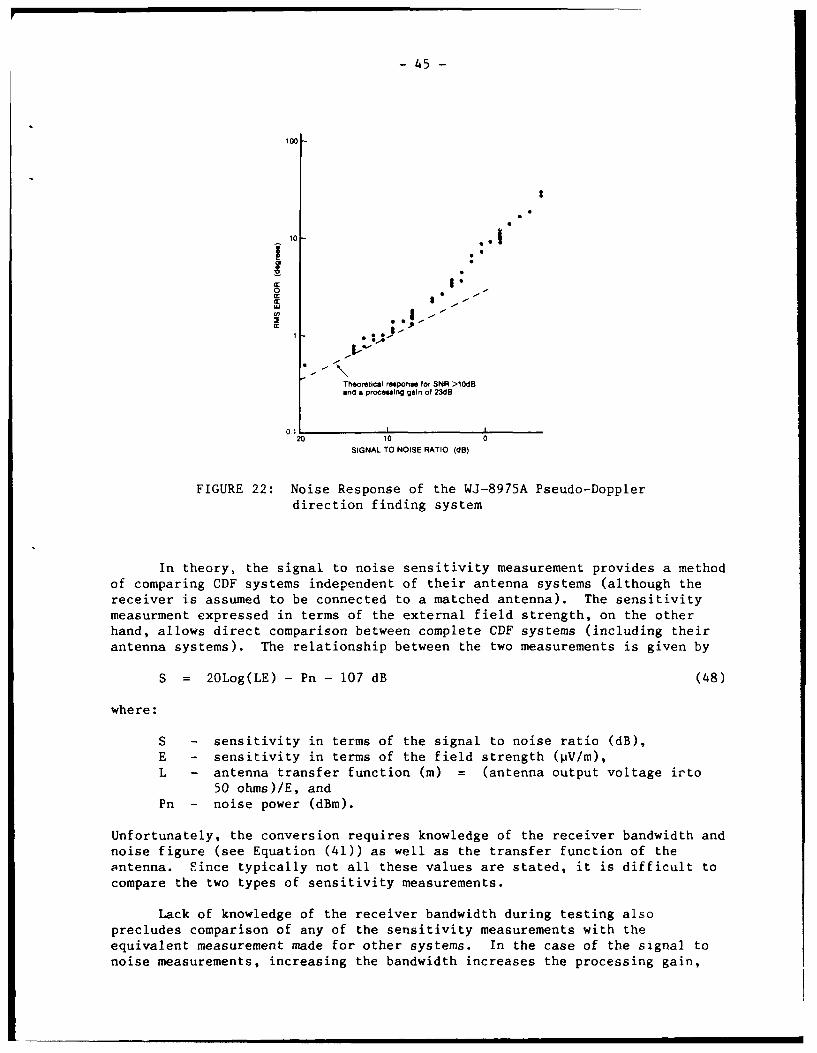
- 45 -
100
10-
CIC.(0 -
Theoretical response for SNy >10dBand a procehsing gain of MISB
0.1 L
20 10SIGNAL TO NOISE RATIO (dB)
FIGURE 22: Noise Response of the WJ-8975A Pseudo-Dopplerdirection finding system
In theory, the signal to noise sensitivity measurement provides a methodof comparing CDF systems independent of their antenna systems (although thereceiver is assumed to be connected to a matched antenna). The sensitivitymeasurment expressed in terms of the external field strength, on the otherhand, allows direct comparison between complete CDF systems (including theirantenna systems). The relationship between the two measurements is given by
S = 20Log(LE) - Pn - 107 dB (48)
where:
S - sensitivity in terms of the signal to noise ratio (dB),E - sensitivity in terms of the field strength (pV/m),L - antenna transfer function (i) = (antenna output voltage irto
50 ohms)/E, andPn - noise power (dBm).
Unfortunately, the conversion requires knowledge of the receiver bandwidth andnoise figure (see Equation (41)) as well as the transfer function of theantenna. Since typically not all these values are stated, it is difficult tocompare the two types of sensitivity measurements.
Lack of knowledge of the receiver bandwidth during testing alsoprecludes comparison of any of the sensitivity measurements with theequivalent measurement made for other systems. In the case of the signal tonoise measurements, increasing the bandwidth increases the processing gain,
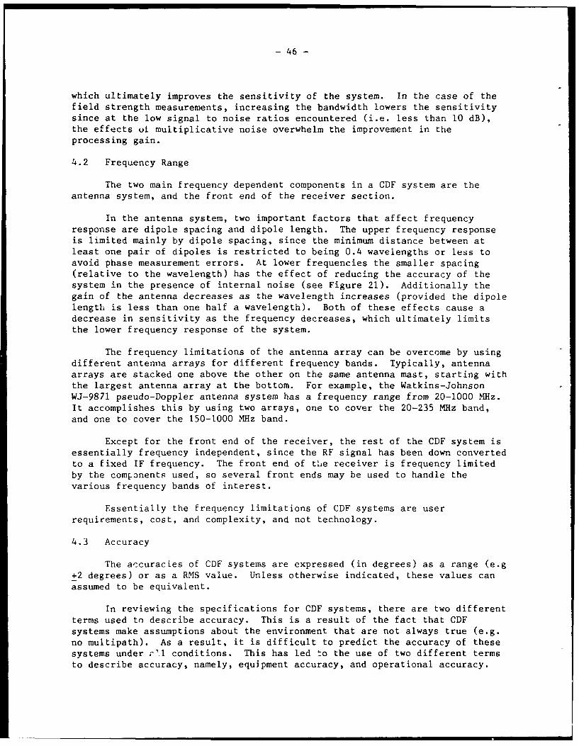
- 46 -
which ultimately improves the sensitivity of the system. In the case of thefield strength measurements, increasing the bandwidth lowers the sensitivitysince at the low signal to noise ratios encountered (i.e. less than 10 dB),the effects oi multiplicative noise overwhelm the improvement in theprocessing gain.
4.2 Frequency Range
The two main frequency dependent components in a CDF system are theantenna system, and the front end of the receiver section.
In the antenna system, two important factors that affect frequencyresponse are dipole spacing and dipole length. The upper frequency responseis limited mainly by dipole spacing, since the minimum distance between atleast one pair of dipoles is restricted to being 0.4 wavelengths or less toavoid phase measurement errors. At lower frequencies the smaller spacing(relative to the wavelength) has the effect of reducing the accuracy of thesystem in the presence of internal noise (see Figure 21). Additionally thegain of the antenna decreases as the wavelength increases (provided the dipolelength is less than one half a wavelength). Both of these effects cause adecrease in sensitivity as the frequency decreases, which ultimately limitsthe lower frequency response of the system.
The frequency limitations of the antenna array can be overcome by usingdifferent antenna arrays for different frequency bands. Typically, antennaarrays are stacked one above the other on the same antenna mast, starting withthe largest antenna array at the bottom. For example, the Watkins-JohnsonWJ-9871 pseudo-Doppler antenna system has a frequency range from 20-1000 MHz.It accomplishes this by using two arrays, one to cover the 20-235 MHz band,and one to cover the 150-1000 MHz band.
Except for the front end of the receiver, the rest of the CDF system isessentially frequency independent, since the RF signal has been down convertedto a fixed IF frequency. The front end of t'ie receiver is frequency limitedby the components used, so several front ends may be used to handle thevarious frequency bands of interest.
Essentially the frequency limitations of CDF systems are userrequirements, cost, and complexity, and not technology.
4.3 Accuracy
The accuracies of CDF systems are expressed (in degrees) as a range (e.g+2 degrees) or as a RMS value. Unless otherwise indicated, these values canassumed to be equivalent.
In reviewing the specifications for CDF systems, there are two differentterms used to describe accuracy. This is a result of the fact that CDFsystems make assumptions about the environment that are not always true (e.g.no multipath). As a result, it is difficult to predict the accuracy of thesesystems under r'l conditions. This has led to the use of two different termsto describe accuracy, namely, equipment accuracy, and operational accuracy.
- 47 -
4.3.1 Equipment kccuracy
The equipment accuracy (also called instrumental accuracy, or systemaccuracy) is a measure of the overall accuracy of all or most of the systemunder ideal environmental conditions (i.e. the assumptions made about theenvironment in Section 2.0 are true).
One method of measuring equipment accuracy is with the use of a bearingsimulator. The bearing simulator injects correctly phased signals into thesystem, effectively bypassing the antenna system, to simulate an RF signalarriving from a known bearing. Comparing the measured bearing with thesimulated bearing gives the bias error. Repeating this procedure at differentfrequencies (and possibly different simulated bearings) results in a set ofbias errors. The equipment accuracy is the RMS value of this set.
Another method of measuring equipment accuracy places the CDF system ona turntable at a site with insignificant multipath or at least knowncharacteristics (i.e. site effects can be corrected for afterwards). A signalfrom a known direction is transmitted to the CDF system and the bearing angleis measured. After accounting for the offset introduced by the turntable, thebias error is computed by comparing the measured bearing to the actual signalbearing. By repeating this procedure for a number of different turntableorientations and frequencies, a whole set of bias errors is generated. As inthe first method, the equipment accuracy is the RMS value of the set of biaserrors.
A disadvantage of the first method is that it does not account forerrors resulting from the antenna system which can be significant.Additionally, the results may only be valid for a single bearing.Consequently, the results tend to be extremely good (e.g. see the PA 555 inTable 1).
The second method does account for the antenna system, but still haslimitations. Normally, the site used to test the accuracy of the system isthe same site used to calibrate the system, so the equipment accuracy resultsare generally reasonably good (e.g. see CELS in Table 1). Unfortunately,since it is difficult to find a site truly free of multipath effects, or aleast be able to account for them, errors can be incorporated into the systemcalibration table which are a function of the site and not the equipment.
4.3.2 Operational Accuracy
The operational accuracy of a CDF system is a measure of the overallaccuracy in a realistic signal environment. However, since it is difficult todefine what a realistic environment is, operational accuracy is rarely listedin specifications.
In tests on CDF systems, operational accuracy h~s been found to be afunction of the environmental conditions, rather than equipment accuracy. Forexample, tests carried out at DREO on the Watkins-Johnson WJ-9871 singlechannel pseudo-Doppler system showed the equipment accuracy (including antennasystem) to be better than 2 degrees at 56.5 MHz and 62.5 MHz. The operationalaccuracy of the system at various sites, however, was found to range from 3 to9 degrees. As a point of interest, this system is specified to have anoperational accuracy of 3 degrees.
- 48 -
When specified, operational accuracy is based on the manufacturersinterpretation of a realistic environment, which is often more optimistic thanrealistic!. Since the interpretation may vary from manufacturer tomanufacturer, a comparison of different systems based on this specificationwould be meaningless.
4.4 Minimum Signal Duration
The minimum signal duration specification provides information on howlong a signal must remain on air before its bearing angle can be measured.This is important when considering the performance of a CDF system againstshort duration signals such as burst or on/off type signals.
One disadvantage of noise filtering is the limitation it places on theresponse time of the CDF system when intercepting short duration signals thatare transmitted for a period of time less than twice the integration timeconstant. Integration of the input information when the signal is absentincreases the amount of noise energy in the the measurement without increasingthe signal energy. This results in a decrease in accuracy.
An example of the results of this effect in a phase interferometersystem are shown in the upper curve of Figure 23. In this case, randombearing errors are caused by internal noise. For short duration signals, whenthe signal is off, the RMS error is so large (103.92 degrees) that it tends tocompletely dominate the overall error unless the on time of the signal is verynearly twice the integration time constant.
A second disadvantage is that even if the signal duration is just longenough, it is unlikely that the operator would be able to pick out a singlegood measurement from a series of random measurements.
The solution used in some CDF systems to solve both these problems is tomake measurements and update the bearing display only when a signal ispresent. The presence of the signal is determined by comparing the inputsignal power to an operator selected threshhold value. For the example, thisresults in the accuracy given by the lower curve in Figure 23. For differentsignal to noise ratios, bandwidths, etc. The results would be expected tovary as discussed in Section 3.8.
From the above discussion it is apparent that the minimum signalduration specification may be as simple as twice the value of the minimumintegration time constant setting. However, if "signal only" integration is afeature of the CDF system, then the signal to noise ratio, input bandwidth,and the minimum acceptable error must also be specified before meaningfulcomparisons can be made between various CDF systems.
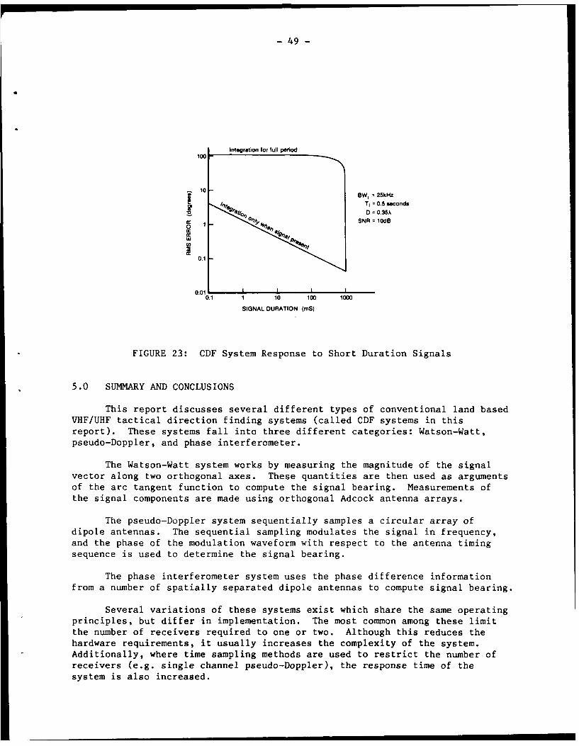
- 49 -
Integratlon for full period100
-~10BW, = 25kHz
Ti = 0.5 secondsD = 0.35A
SNR = 10dSO 0%
0
0.1
0.01 I I I0.1 1 10 100 1000
SIGNAL DURATION (mS)
FIGURE 23: CDF System Response to Short Duration Signals
5.0 SUMMARY AND CONCLUSIONS
This report discusses several different types of conventional land basedVHF/UHF tactical direction finding systems (called CDF systems in thisreport). These systems fall into three different categories: Watson-Watt,pseudo-Doppler, and phase interferometer.
The Watson-Watt system works by measuring the magnitude of the signalvector along two orthogonal axes. These quantities are then used as argumentsof the arc tangent function to compute the signal bearing. Measurements ofthe signal components are made using orthogonal Adcock antenna arrays.
The pseudo-Doppler system sequentially samples a circular array ofdipole antennas. The sequential sampling modulates the signal in frequency,and the phase of the modulation waveform with respect to the antenna timingsequence is used to determine the signal bearing.
The phase interferometer system uses the phase difference informationfrom a number of spatially separated dipole antennas to compute signal bearing.
Several variations of these systems exist which share the same operatingprinciples, but differ in implementation. The most common among these limitthe number of receivers required to one or two. Although this reduces thehardware requirements, it usually increases the complexity of the system.Additionally, where time sampling methods are used to restrict the number ofreceivers (e.g. single channel pseudo-Doppler), the response time of thesystem is also increased.
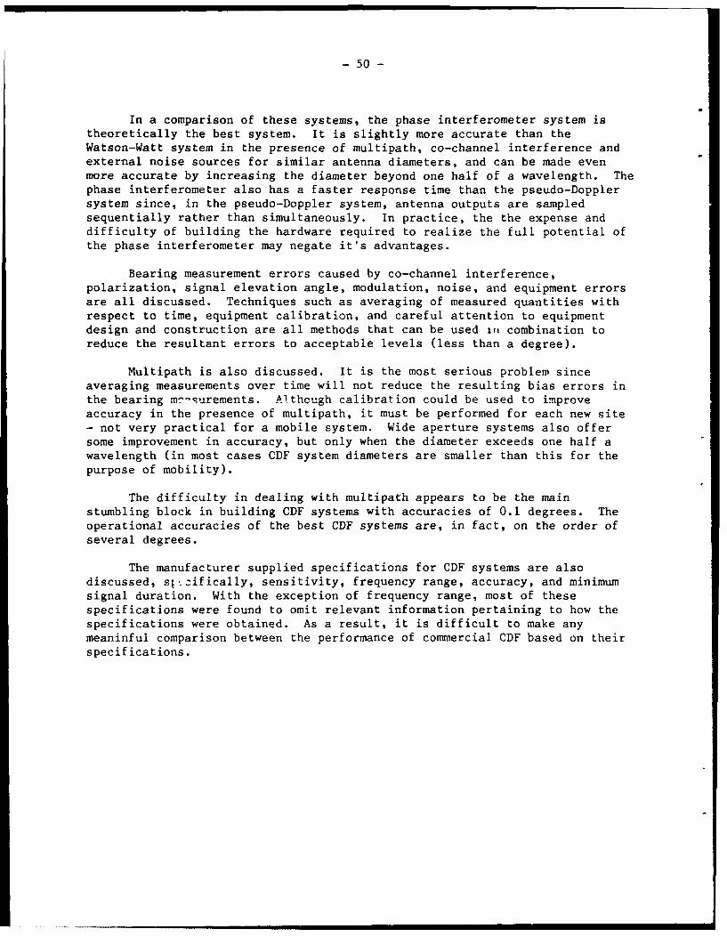
- 50 -
In a comparison of these systems, the phase interferometer system istheoretically the best system. It is slightly more accurate than theWatson-Watt system in the presence of multipath, co-channel interference and
external noise sources for similar antenna diameters, and can be made evenmore accurate by increasing the diameter beyond one half of a wavelength. Thephase interferometer also has a faster response time than the pseudo-Doppler
system since, in the pseudo-Doppler system, antenna outputs are sampled
sequentially rather than simultaneously. In practice, the the expense anddifficulty of building the hardware required to realize the full potential ofthe phase interferometer may negate it's advantages.
Bearing measurement errors caused by co-channel interference,
polarization, signal elevation angle, modulation, noise, and equipment errors
are all discussed. Techniques such as averaging of measured quantities withrespect to time, equipment calibration, and careful attention to equipment
design and construction are all methods that can be used in combination toreduce the resultant errors to acceptable levels (less than a degree).
Multipath is also discussed. It is the most serious problem sinceaveraging measurements over time will not reduce the resulting bias errors inthe bearing mt-;urements. Although calibration could be used to improve
accuracy in the presence of multipath, it must be performed for each new site- not very practical for a mobile system. Wide aperture systems also offer
some improvement in accuracy, but only when the diameter exceeds one half awavelength (in most cases CDF system diameters are smaller than this for the
purpose of mobility).
The difficulty in dealing with multipath appears to be the mainstumbling block in building CDF systems with accuracies of 0.1 degrees. The
operational accuracies of the best CDF systems are, in fact, on the order ofseveral degrees.
The manufacturer supplied specifications for CDF systems are also
discussed, sv :ifically, sensitivity, frequency range, accuracy, and minimumsignal duration. With the exception of frequency range, most of these
specifications were found to omit relevant information pertaining to how thespecifications were obtained. As a result, it is difficult to make anymeaninful comparison between the performance of commercial CDF based on their
specifications.
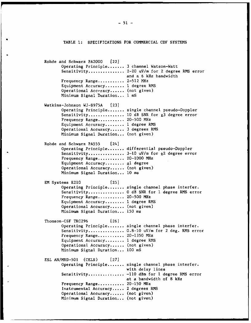
- 51 -
TABLE 1: SPECIFICATIONS FOR COMMERCIAL CDF SYSTEMS
Rohde and Schwarz PA2000 [22]
Operating Principle ....... 3 channel Watson-Watt
Sensitivity ............... 2-20 uV/m for 2 degree RMS error
and a 6 kHz bandwidthFrequency Range ........... 2-512 MHz
Equipment Accuracy ........ I degree RMS
Operational Accuracy ...... (not given)
Minimum Signal buration... I mS
Watkins-Johnson WJ-8975A [23]Operating Principle ....... single channel pseudo-Doppler
Sensitivity ............... 10 dB SNR for ±3 degree errorFrequency Range ........... 20-500 MHz
Equipment Accuracy ........ I degree RMS
Operational Accuracy ...... 3 degrees RMS
Minimum Signal Duration... (not given)
Rohde and Schwarz PA555 [24]Operating Principle ....... differential pseudo-Doppler
Sensitivity ............... 3-10 uV/m for ±2 degree errorFrequency Range ........... 20-1000 MHz
Equipment Accuracy ........ ±1 degree
Operational Accuracy ...... (not given)
Minimum Signal Duration... 10 ms
EM Systems E210 [25]
Operating Principle ....... single channel phase interfer.Sensitivity ............... 0 dB SNR for I degree RMS errorFrequency Range ........... 20-500 MHz
Equipment Accuracy ........ 1 degree RMS
Operational Accuracy ...... (not given)
Minimum Signal Duration... 150 ms
Thomson-CSF TRC296 [26]
Operating Principle ....... single channel phase interfer.Sensitivity ............... 0.8-10 uV/m for 2 deg. RMS errorFrequency Range ........... 20-1350 MHzEquipment Accuracy ........ 1 degree RMS
Operational Accuracy ...... (not given)
Minimum Signal Duration... 100 mS
ESL AN/MRD-501 (CELS) [27]Operating Principle ....... single channel phase interfer.
with delay lines
Sensitivity ............... -110 dBm for i degree RMS errorat a bandwidth of 8 kHz
Frequency Range ........... 20-150 MHzInstrumental Accuracy ..... 2 degrees RMS
Operational Accuracy ...... (not given)Minimum Signal Duration... (not given)
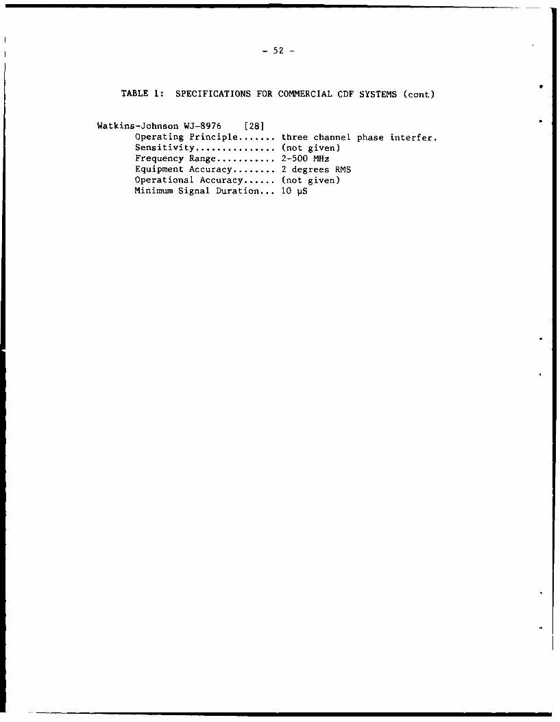
- 52 -
TABLE 1: SPECIFICATIONS FOR COMMERCIAL CDF SYSTEMS (cont)
Watkins-Johnson WJ-8976 (281Operating Principle ....... three channel phase interfer.Sensitivity ............... (not given)Frequency Range ........... 2-500 MHzEquipment Accuracy ........ 2 degrees RMSOperational Accuracy ...... (not given)Minimum Signal Duration... 10 pS

- 53 -
6.0 REFERENCES
[I] Watson Watt, R.A., and Herd, J.F., "An Instantaneous Direct-ReadingRadiogoniometer" , lEE, Vol. 64, pp. 611-617, 1926
[21 Earp, C.W., and Godfrey, R.M., "Radio Direction-Finding by the CyclicalDifferential Measurement of Phase", lEE, Vol. 94, Part Ilia, pp.705-721, 1947.
[3] McLeish, C.W., and Burtnyk N., "The Application of the Interferometer toH.F. Direction Finding", lEE, Vol. 108B, pp. 495-499, 1961.
[41 Cleaver, R.F., "The Development of Single Receiver Automatic AdcockDirection Finders for use in the Frequency Band 100-150 Megacycles perSecond", lEE, Vol. 94, Part Ilia, pp. 783-799, 1947.
[5] Rainer, R., and Burwasser, A.J., "An Approach to HF Tactical RadioDirection Finding and Signal Monitoring", Journal of Electronic Defence,pp. 173-184, October, 1983.
[6] Oeh, G., and Lampell, A., "Advanced Techniques Give One-Degree Accuracyin VHF/UHF Direction Finding", MSN, pp. 145-157, March, 1984.
[7] "AN/TSQ-114B DF Collection Algorithm Description", ESL Internal Report,California.
[8] Mike Davis, Private Communication, ESL, California.
[9] Steiner, F., "Wide-Base Doppler Very-High-Frequency Direction Finder",IRE, Vol. ANE-7, pp 98-105, September, 1960.
[10] "PA 007, PA 008 and PA 009 VHF/UHF Doppler Direction Finders", TechnicalData Sheet, Rohde and Schwarz, Germany.
[11] Hopkins, H.G., and Horner, F., "Direction Finding Site Errors at VeryHigh Frequencies", lEE. Vol. 96, Part III, pp 321-332, 1949.
[12] Horner, F., "An Investigation of Polarization Errors in an H-AdcockDirction-Finder", lEE, Vol. 99, Part IV, pp. 229-240, 1954.
[13] Harrington, J.B., "Direction-Finding in Tactical Communications isConstrained by Topography, not Technology", MSN, pp. 64-78, August, 1983.
[14] Travers, D.N., "The Effect of Mutual Impedance on the Spacing Error ofan Eight-Element Adcock", IRE Transactions on Antennas and Propagation,Vol. 4, pp.36-39, January, 1957.
[15] "UHF Frequency Extension Study", ESL Report No. ESL-87-0027, California,March, 1987.
[16] Mumford, W.W., and Scheibe, E.H., "Noise Performance Factors inCommunication Systems, Horizon House, Dedham, Massachusettes, 1968.
t ei
- 54 -
[17] Gregorian, R., and Temes, G.C., "Analog MOS Integrated Circuits forSignal Processing", John Wiley and Sons, Toronto, Canada, 1986.
[181 Roberts, J.H., "Envelope and Phase Statistics for Non-Gaussian Noise andResulting Error Probabilities for Digital Communications Systems", AGARDConference Preprint, No. 407, pp. 19-1 to 19-14, 1986.
[19] Spaulding, A.D., "Stochastic Modelling of the ElectromagneticInterference Environment", IEEE, ICC 77 (Chicago), pp. 42.2-114 to42.2-123, 1977.
[20] Stremler, F.G., "Introdution to Communication Systems", Adison-WesleyPublishing Company, Toronto, Canada, pp. 159-161, 1977.
[21] Ksienski, A., "A Survey of Signal Processing Arrays", AGARD ConferenceProceedings on Signal Processing Arrays, no. 16, pp. 1-44, July 1966.
[22] "Integrated Signal Interception System PA 2000", Technical Data Sheet,Rohde and Schwarz, Germany.
[23] "WJ-8975A Manpack Direction Finder Processor", Technical Data Sheet,Watkins-Johnson Company, Maryland, February, 1982.
[241 "Mobile VHF-UHF Broadband Doppler Direction Finder PA 555", TechnicalData Sheet, Rohde and Schwarz, Germany.
[25] "E210 System Direction Finding Equipment - 20 to 500 MHz", TechnicalData Sheet, EM Systems Inc., California
[26] "TRC 296 20-1350 MHz Radio Direction Finder", Technical Data Sheet,Thomson-CSF, France, October, 1985.
[27] "CELS Acceptance Test Procedure", ESL 70-168902, California, January,1987.
[28] "WJ-8976 Three Channel Direction Finding System", Technical Data Sheet,Watkins-Johnson Company, Maryland, January, 1986.
[29] Jacobs, E. and Ralston, E.W., "Ambiguity Resolution in Interferometry",IEEE Transactions on Aerospace and Electronic Systems, Vol 17, No. 6, pp766-780, November 1981.
UNCLASSIFIED - 55 -
SECURITY CLASSIFICATION OF FORM(highest classification of Title, Abstract, Keywords)
DOCUMENT CONTROL DATA(Security classification of title, body of abstract end indexing annotation must be entered when the . document is classified)
1. ORIGINATOR (the name and address of the organization preparing ti. document 2. SECURITY CLASSIFICATIONOrganizations for whom the document was prepared, e.g. Establishment ,ponsoring (overall security classification of the documenta contractor's report, 3r tasking agency, are entered in section 8.) including special warning terms if applicable)
DEkENCE RESEARCH ESTABLISHMENT OTTAWA
NATIONAL DEFENCESHIRLEY BAY, OTTAWA, ONTARIO KIA OK2 CANADA UNCLASSIFIED
3. TITLE (the complete document title as indicated on the title page. Its classification should be indicated by the appropriateabbreviation (SC,R or U) in parentheses after the title.)
REVIEW OF CONVENTIONAL TACTICAL RADIO DIRECTION FINDING SYSTEMS (U)
4. AUTHORS (Last name, first name, middle initial. If military, show rank, e.g. Doe, Maj. John E.)
READ, William, J.L.
5. DATE OF PUBLICATION (month and year of publication of 6a NO. OF PAGES (total 6b. NO. OF REFS (total cited indocument) containing information. Include document)
Annexes, Appendices, etc.)
54 29
6. DESCRIPTIVE NOTES (the category of the document, e.g. technical report, technical note or memorandum. If appropriate, enter the type ofreport, e.g. interim, progress, summary, annual or final. Give the inclusive dates when a specific reporting period is covered.)
DREO TECHNICAL NOTE
8. SPONSORING ACTIVITY (the name of the department project office or laboratory sponsoring the research and development Include theaddress.)
DEFENCE RESEARCH ESTABLISHMENT OTTAWANATIONAL DEFENCESHIRLEY BAY, OTTAWA, ONTARIO KIA OK2 CANADA
9& PROJECT OR GRANT NO. fif appropriate, the applicable research 9b. CONTRACT NO. (if appropriate, the applicable number underand developmen: project c. grant number under which the document which the document was written)was written. Please specify whether project or grant)
041LKI1
10a. ORIGINATOR'S DOCUMENT NUMBER (the official document 10b. OTHER DOCUMENT NOS. (Any other numbers which maynumber by which the document is identified by the originating be assigned this document either by the originator or by theactivity. This number must be unique to this document) sponsor)
1 1. DOCUMENT AVAILABILITY (any limitations on further dissemination of the document, other than those imposed by security classification)
Oi Unlimited distributionDistribution limited to defence departments and defence contractors; further distribution only as approved
( ) Distribution limited to defence departments and Canadian defence contractors; further distribution only as approvedI I Distribution limited to government departments and agencies; further distribution only as approved
i Ostribution limited to defence departments; further distribution only as approved
( Other (please specify):
12. DOCUMENT ANNOUNCEMENT (any limitation to the bibliographic announcement of this document. This will normally correspond tothe Document Availabilty (11). However, where further distr tion (beyond the audience specified in 11) is possible, a widerannouncement audience may be selected.)
UNCLASSIFIED
SECURITY CLASSIFICATION OF FORM
DCD03 2106/87
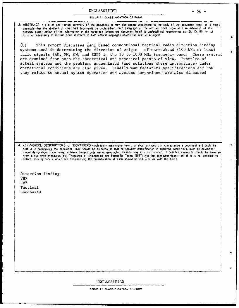
UNCLASSIFIED - 56 -
SECURITY CLASSIFICATION OF FORM
13. ABSTRACT ( a brief and factual summary of the document It may also appear elsewhere in the body of the document itself. It is highlydesirable that the abstract of classified documents be unclassified. Each paragraph of the abstract shall begin with an indication of thesecurity classification of the information in the paragraph (unless the document itself is unclassified) represented as (S), (C), (R), cr VIt is not necessary to include here abstracts in both offical languages unless the text is bilingual).
(U) This report discusses land based conventional tactical radio direction findingsystems used in determining the direction of origin of narrowband (100 kHz or less)radio signals (AM, FM, CW, and SSB) in the 30 to 1000 MHz frequency band. These systemsare examined from both the theoretical and practical points of view. Examples ofactual systems and the problems encountered (and solutions where appropriate) underoperational conditions are also given. Finally manufacturers specifications and howthey relate to actual system operation and systems comparisons are also discussed
14. KEYWORDS, DESCRIPTORS or IDENTIFIERS (technically meaningful terms or short phrases that characterize a document and could behelpful in cataloguing the document They should be selected so that no security ctassification is required. Identifiers, such as equipmentmodel designation, trade name, military project code name, geographic location may also be included. If possible keywords should be selectedfrom a Published tesaurus. e.g. Thesaurus of Engineering and Scientific Terms (TEST) --d that thesaurus-identified. If it is not possible toselect indexing terms which are Unclassified, the classification of each should be indi.Laed as with the ttle.)
Direction finding
VHFUHF
Tactical
Landbased
UNCLASSIFIED
SECURITY CLASSIFICATION OF FORM


![Tactical Combat Casualty Care [TCCC] Some reminders and ...€¦ · Tactical Combat Casualty Care Tactical Evacuation Care The term “Tactical Evacuation” includes both Casualty](https://img.pdfslide.net/doc/110x75/604ef4767ef6a83727287be2/tactical-combat-casualty-care-tccc-some-reminders-and-tactical-combat-casualty.jpg)